| Issue |
A&A
Volume 645, January 2021
|
|
|---|---|---|
| Article Number | A94 | |
| Number of page(s) | 20 | |
| Section | Interstellar and circumstellar matter | |
| DOI | https://doi.org/10.1051/0004-6361/202039353 | |
| Published online | 19 January 2021 | |
Mass segregation and sequential star formation in NGC 2264 revealed by Herschel★,★★
1
Instituto de Radioastronomía y Astrofísica, Universidad Nacional Autónoma de México,
Apdo. Postal 3-72,
58089 Morelia,
Michoacán,
Mexico
e-mail: t.nony@irya.unam.mx
2
Univ. Grenoble Alpes, CNRS, IPAG,
38000 Grenoble,
France
3
AIM, CEA, CNRS, Université Paris-Saclay, Université Paris Diderot, Sorbonne Paris Cité,
91191 Gif-sur-Yvette,
France
4
School of Physics and Astronomy, University of Exeter,
Stocker Road,
Exeter, EX4 4QL,
UK
5
Physikalisches Institut, Universität zu Köln,
Zülpicher Str. 77,
50937 Köln,
Germany
6
School of Physics and Astronomy, University of Leeds,
Leeds LS2 9JT,
UK
7
Laboratoire d’astrophysique de Bordeaux, Univ. Bordeaux, CNRS, B18N, allée Geoffroy Saint-Hilaire,
33615 Pessac,
France
8
INAF – Istituto di Astrofisica e Planetologia Spaziali (IAPS),
via Fosso del Cavaliere 100,
00133 Roma,
Italy
Received:
7
September
2020
Accepted:
11
November
2020
Context. The mass segregation of stellar clusters could be primordial rather than dynamical. Despite the abundance of studies of mass segregation for stellar clusters, those for stellar progenitors are still scarce, so the question concerning the origin and evolution of mass segregation is still open.
Aims. Our goal is to characterize the structure of the NGC 2264 molecular cloud and compare the populations of clumps and young stellar objects (YSOs) in this region whose rich YSO population has shown evidence of sequential star formation.
Methods. We separated the Herschel column density map of NGC 2264 into three subregions and compared their cloud power spectra using a multiscale segmentation technique. We extracted compact cloud fragments from the column density image, measured their basic properties, and studied their spatial and mass distributions.
Results. In the whole NGC 2264 cloud, we identified a population of 256 clumps with typical sizes of ~0.1 pc and masses ranging from 0.08 M⊙ to 53 M⊙. Although clumps have been detected all over the cloud, most of the massive, bound clumps are concentrated in the central subregion of NGC 2264. The local surface density and the mass segregation ratio indicate a strong degree of mass segregation for the 15 most massive clumps, with a median Σ6 three times that of the whole clumps population and ΛMSR ≃ 8. We show that this cluster of massive clumps is forming within a high-density cloud ridge, which is formed and probably still fed by the high concentration of gas observed on larger scales in the central subregion. The time sequence obtained from the combined study of the clump and YSO populations in NGC 2264 suggests that the star formation started in the northern subregion, that it is now actively developing at the center, and will soon start in the southern subregion.
Conclusions. Taken together, the cloud structure and the clump and YSO populations in NGC 2264 argue for a dynamical scenario of star formation. The cloud could first undergo global collapse, driving most clumps to centrally concentrated ridges. After their main accretion phase, some YSOs, and probably the most massive, would stay clustered while others would be dispersed from their birth sites. We propose that the mass segregation observed in some star clusters is inherited from that of clumps, originating from the mass assembly phase of molecular clouds.
Key words: ISM: structure / stars: formation / methods: statistical / open clusters and associations: individual: NGC 2264 / ISM: clouds
Table A.1 is only available at the CDS via anonymous ftp to cdsarc.u-strasbg.fr (130.79.128.5) or via http://cdsarc.u-strasbg.fr/viz-bin/cat/J/A+A/645/A94
© ESO 2021
1 Introduction
Among the major open questions in the field of stellar cluster formation today is defining whether stellar properties, and especially their clustering characteristics and dynamical state, could be inherited from the properties of the clouds themselves. Mass segregation has been studied extensively in stellar clusters for decades to investigate if the energy equipartition associated with two-body relaxation (Spitzer 1969) causes high-mass stars to fall toward the center of mass of clusters. As a matter of fact, mass segregation has been observed, as expected, in dynamically old globular and open clusters, but also in very young regions, suggesting it was not due to dynamical evolution (see, e.g the review by Meylan 2000, and references therein). Primordial mass segregation prompts the question of whether there are preferential sites for high-mass star formation (Murray & Lin 1996) or whether the observed segregation is related to energy equipartition at all (e.g., Parker et al. 2016). Simulations indicate that primordial structure, if present, can be rapidly erased through dynamical interactions of the stars and expulsion of the gas (Parker & Meyer 2012; Fujii & Portegies Zwart 2016). Observational studies, however, show a weak, if any, correlation between thesubstructure and the age of the stellar clusters (Sánchez & Alfaro 2009; Dib et al. 2018). Hetem & Gregorio-Hetem (2019) indicate that stellar clusters did not significantly change in terms of structure within their first 10 Myr, and corroborate the absence of correlation between mass segregation and the age of clusters, as initially reported by Dib et al. (2018). Specifically, measuring the spatial distribution and mass segregation of molecular cloud fragments and comparing these properties to that of young stellar objects (YSOs) is essential to study this link. A handful of studies have started investigating the mass segregation of molecular cores (Plunkett et al. 2018; Dib & Henning 2019; Román-Zúñiga et al. 2019), mostly focusing, first, on low-mass star-forming regions.
The Herschel observatory imaged, with an unprecedented sensitivity and angular resolution, the low- to high-mass star-formingclouds located at 100–500 pc and 0.7–3 kpc from the Sun (André et al. 2010; Motte et al. 2010). These surveys provide the opportunity to build large, if not complete, catalogs of cloud fragments with sizes of 0.01–0.1 pc (qualified of cores) to 0.1–1 pc (called clumps). At these scales, clumps likely fragment into cores, which could themselves be the direct progenitors of stars or small stellar systems. The Herschel imaging survey of OB young stellar objects (HOBYS1; Motte et al. 2010) is the first systematic survey of a complete sample of nearby molecular cloud complexes forming high-mass stars. The wide-field photometric imaging, performed with both the SPIRE and PACS cameras of Herschel, aims to complete the census of high-mass star progenitors at 0.1 pc scales in essentially all the molecular cloud complexes at less than 3 kpc. The HOBYS sample contains seven massive (3 × 10⁵ to 3 × 10⁶ M⊙) molecular complexes at 1.4–3 kpc from the Sun, including Cygnus X and NGC 6334, and two intermediate-mass, a few 105 M⊙, cloud complexes at 0.7–0.8 kpc, Vela C and Monoceros (Mon R1, Mon R2, NGC 2264).
Notably, HOBYS revealed a tight link between the density, dynamics, and clump population of the so-called ridges (Motte et al. 2018). The latter are high-density filaments (n > 105 cm−3 over ~5 pc3) forming clusters of high-mass stars (e.g., Schneider et al. 2010; Hill et al. 2011; Nguyen Luong et al. 2011, 2013; Hennemann et al. 2012; Tigé et al. 2017), whereas hubs are more spherical smaller structures forming at most a couple of high-mass stars (e.g., Schneider et al. 2012; Peretto et al. 2013; Rivera-Ingraham et al. 2013; Didelon et al. 2015; Rayner et al. 2017). The existence of ridges and hubs is predicted by dynamical models of cloud formation such as colliding flow or gravitationally driven gas inflows simulations (e.g., Heitsch et al. 2008; Smith et al. 2009; Hartmann et al. 2012) and some analytical theories of filament collapse/conveyor belt (Myers 2009; Krumholz & McKee 2020).
The Monoceros OB1 (Mon OB1) cloud complex is located at a Gaia DR2 determined distance of 723 pc (Cantat-Gaudin et al. 2018). In the mid-infrared, this cloud complex displays a 2.5° (~30 pc) diameter half loop (Schwartz 1987), of which three 10 pc clouds have been imaged by Herschel as part of the HOBYS and Galactic Cold Cores key programs (Motte et al. 2010; Juvela et al. 2012). NGC 2264 and G202.3 + 2.5 lie at the eastern extremity of Mon OB1; Monoceros R1 is in the west. NGC 2264 is the best-studied cloud of the Mon OB1 complex (see the review by Dahm 2008). Over the past decade, a population of more than 1000 YSOs at various evolutionary stages has been revealed (Teixeira et al. 2012; Povich et al. 2013; Rapson et al. 2014; Venuti et al. 2018). The NGC 2264 cloud is elongated in the NW-SE direction, with a gradient of star formation observed for YSOs from north to south (Sung & Bessell 2010; Venuti et al. 2018). NGC 2264 hosts the massive O7-type binary star S Monocerotis (S Mon), in the north, and the famous Cone Nebula, a triangular projection of molecular gas lying ~8 pc south of S Mon. The YSO population of NGC 2264 is mainly distributed in three subclusters: a cluster of pre-main sequence stars in the north, in the vicinity of S Mon (Sung et al. 2009), and two clusters in the center. The central subclusters are often labeled according to their dominant objects, NGC 2264-IRS1, a B2-type star also known as Allen’s source and -IRS2, a Class I protostar. IRS1 and IRS2 areas are also referred as NGC 2264-C and -D, or the Spokes cluster for NGC 2264-IRS2 region (Teixeira et al. 2006). These regions are still active sites of star formation, with many embedded Class 0/I protostars observed in millimeter continuum and lines (Williams & Garland 2002; Peretto et al. 2006; Young et al. 2006; Cunningham et al. 2016). Gas motions have also been reported from large scales, like the global collapse of NGC 2264-C (Williams & Garland 2002; Peretto et al. 2006), to small scales like protostellar outflows (Maury et al. 2009; Cunningham et al. 2016).
The paper is organized as follows. We introduce, in Sect. 2, the Herschel column density map and clump catalog of the NGC 2264 cloud. In Sect. 3, we analyze the cloud structure using a multiscale decomposition tool and divide the NGC 2264 cloud into three subregions. We then compare, in Sect. 4, the physical properties of clumps in these subregions and discuss their spatial distribution and mass segregation. In Sect. 5, we compare the YSO and clump populations, in Sect. 6 we discuss mass segregation and propose a revised history for star formation in the NGC 2264 cloud. Finally, we summarize our conclusions in Sect. 7.
2 NGC 2264 data set
2.1 Herschel images, derived column density, and temperature maps
NGC 2264 was observed by the Herschel space observatory with the PACS (Poglitsch et al. 2010) and SPIRE (Griffin et al. 2010) instruments as part of the HOBYS (Motte et al. 2010) Key Program (OBSIDs: 1342205056 and 1342205057). Data were taken in five bands: 70 and 160 μm for PACS and 250, 350, and 500 μm for SPIRE with full width at half maximum (FWHM) resolutions of 5.9′′, 11.7′′, 18.2′′, 24.9′′, and 36.3′′, respectively. Observations were performed in parallel mode, using both instruments simultaneously, with a scanning speed of 20′′ s−1. This results in a common PACS and SPIRE area of 1.0° × 1.2°, which corresponds to 10 pc × 13 pc at a distance of 723 pc.
The data were reduced using the Herschel Interactive Processing Environment (HIPE; Ott 2010) software, version 10.0.2751. The SPIRE nominal and orthogonal maps were separately processed and subsequently combined and reduced for de-stripping, relative gains, and color correction with HIPE. The PACS maps were reduced with HIPE up to Level 1 and, from there up to their final version (Level 3), using Scanamorphos v21.0 (Roussel 2013). The composite three-color (RGB = 250 μm/160 μm/70 μm) Herschel image of the NGC 2264 cloud is presented in Fig. 1.
High-resolution column density and temperature images, at the 18.2′′ resolution of the 250 μm image, were built using the methods presented in Palmeirim et al. (2013) and Men’shchikov (2020). In short, we fitted pixel-by-pixel spectral energy distributions of the Herschel images with modified blackbody models to four, three, and two wavelengths (160/250/350/500 μm, 160/250/350 μm, and 160/250 μm) that were convolved to the lowest resolution of the images available in the three sets of wavebands. The higher-resolution information contained inthe resulting density images, obtained with the smaller number of wavelengths, was transferred differentially to the 36′′ resolution density image derived by fitting four wavebands, thereby increasing its resolution by a factor of two. We adopted a power-law approximation to the dust opacity law per unit of mass at submillimeter wavelengths,  cm2 g−1, assuming a dust emissivity index β = 2 and a gas-to-dust ratio of 100. The resulting column density and dust temperature images are presented in Figs. 2 and A.1. The column density map traces cloud structures from ~ 2 × 1021 cm−2 to 2.7 × 1023 cm−2. The main cloud structure above ~ 4 × 1021 cm−2 displays a “Y” shape and consists of a hub of three filaments connecting toward a NW-SE ridge. The highest column densities,
  cm−2, are reached at the center of NGC 2264, toward the two protostellar clusters NGC 2264-IRS1 and IRS2. Most of the gas at low to medium column density has a dust temperature of ~ 14.5 K, decreasing down to 11–12 K within some high-density filaments and increasing up to 20–24 K toward IRS1 and IRS2. In the north, a large bubble of low-density, heated gas, with 18–27 K over ~ 4 pc, is associated with a rosette-shaped nebula observed in infrared and a couple of OB stars including the Herbig Ae/Be star called W90 (Dahm 2008).
Since Mon OB1 lies above the Galactic plane, the contamination of Herschel column density and temperature images by other clouds along the same line of sight is minimal (see Schneider et al., in prep. for a complete discussion of contamination effects). Absolute uncertainties on  (a factor of 2) and Tdust (a few degrees) depend mostly on the assumption taken for the dust mass opacity.
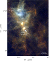 |
Fig. 1 Composite three-color Herschel image of NGC 2264: PACS 70 and 160 μm in blue and green; SPIRE 250 μm in red. The massive star S Mon, the central protoclusters NGC 2264 IRS1 and IRS2 and the Cone Nebula are labeled. The blue component traces heated regions while earlier stage star-forming sites, such as clumps and filaments, are traced by the red component. The image has been rotated from the RA–Dec grid. |
2.2 Clump catalog
Compact sources were extracted from the column density map at 18.2′′ resolution (see Sect. 2.1) using getsf (v200124, Men’shchikov 2020), a new multi-scale, multi-wavelength source and filament extraction algorithm based on the separation of structural components. The method is a major improvement over its predecessors getsources, getfilaments, and getimages (Men’shchikov et al. 2012; Men’shchikov 2013, 2017). Original images are spatially decomposed into a set of 99 single-scale images, from two pixels to a maximum scale of four times the maximum size of sources of interest, 5.6′′ –232′′ (or 0.8 pc) for the NGC 2264 HOBYS field. The decomposed images are processed and analyzed by getsf to separate three structural components – sources, filaments, and background. The method flattens the sources and filament components to equalize their noise and background fluctuations to reliably detect sources and filaments using intensity (here, column density) thresholds.
Detection of sources and filaments is done in the single-scale flattened images, whereas their measurements are done in the background-subtracted original image. The resulting catalog contains, for each extracted source, its peak and integrated column densities,  and
and  , with uncertainties; its major and minor axis sizes at FWHM, A and B; and the position angle of its elliptical footprint (PA). Also given is the source detection significance, S, which is a single-scale analog of the signal-to-noise ratio (S/N) and the column density of the subtracted background,
  . To measure this background column density, we averaged the background map provided by getsf over the source FWHM. A subset of this catalog is given in Table 1 and the complete table is available in electronic form through CDS.
We also list in Table 1 the source FWHM sizes deconvolved from the beam, FWHMdec, which provide an estimation of the physical sizes and range from 0.03 to 0.2 pc with a median value of 0.11 pc. The source average dust temperatures, Tdust, are listed with their associated uncertainties. These parameters are defined as the mean and dispersion, respectively, measured over the source FWHM areas on the temperature map of Fig. A.1. The measured temperature are averaged along the line of sight of each clump and generally overestimate by a few degrees the mean dust temperature of cold, shielded clumps (Hill et al. 2012). The Tdust ranges from 11.5 to 22.7 K with a median of 13.9 K. The temperature distribution in Fig. A.4 show little variations, as 85% of the clumps have a temperature between 12 and 16 K.
A total of 256 sources have been extracted in NGC 2264 using getsf; these are plotted over the column density map in Figs. 2, 3. The mass of the clumps is calculated from the integrated column density given by getsf,  (see Table 1), following the equation:
 (1)
(1)
where  the molecular weight per hydrogen molecule, mH the hydrogen mass, d = 723 pc the distance to NGC 2264, and Ωb the beam solid angle. Masses range from 0.08 M⊙ to 53 M⊙ with a median of 0.9 M⊙. The relative uncertainty of clump masses is estimated to be less than 50%, but the absolute uncertainty could be of a factor of 2.
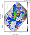 |
Fig. 2 NGC 2264 cloud traced by its Herschel column density. The clumps extracted by getsf are indicated by hatched ellipses for gravitationally bound clumps and open ellipses empty for unbound clumps. The contour at 2 × 1022 cm−2 highlights the brightest parts. The resolution of the map, 18.2′′, is shown in the lower right corner and a scale bar is given in the upper left corner. The outline and labels of the three subregions defined in Sect. 3.1 and used in the analysis are shown in red. The location of the zoom of Fig. 3 is shown with a white box. |
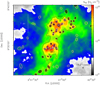 |
Fig. 3 Zoom toward the central part of NGC 2264 imaged through its Herschel column density. Same caption as Fig. 2. The white and black crosses show the location of the NGC 2264 IRS1 and IRS2 sources, respectively. The associated IRS1 and IRS2 protoclusters contain most of the gravitationally bound clumps of this NGC 2264 subregion. The 15 most massive clumps (M > 9.3 M⊙) are pinpointed with their number, the 16th clump is located outside this zoom. |
Sample catalog of clumps identified in NGC 2264 using the Herschel column density map.
2.3 YSO catalog
We selected the YSOs from the 2MASS/Spitzer catalog established by Rapson et al. (2014) on the eastern part of the Mon OB1 molecular complex. The Spitzer map used by Rapson et al. (2014) covers most of the Herschel field, except for small areas in the south, east, and west, within which ten clumps have been detected. Other YSO catalogs built over smaller areas (like that of, e.g., Kuhn et al. 2014) or combining spectroscopic and photometric data (Venuti et al. 2018) are not used in this workso as to maintain the homogeneity of the YSO catalog. Rapson et al. (2014) used Spitzer IRAC (3.6–8 μm) and MIPS 24 μm data to select YSOs based on their IR excess. This sample thus includes class 0/I sources, while that of Cody et al. (2014) does not since they use only IRAC data.
Among the 6381 YSOs within the field of view of the Herschel column density map, there are 87 Class 0/I protostars and 398 Class II pre-main sequence stars. Class III sources have been excluded from the studied sample because being evolved YSOs, they are lessrelevant for comparison with the gas distribution. Besides, the Class III population in the catalog of Rapson et al. (2014) is significantly contaminated with field stars. The classification of YSOs was carried out by Rapson et al. (2014) using a color-based method developed by Gutermuth et al. (2009). Our sample also does not include the ~ 20 intermediate- and high-mass sources that started forming a few 106 yr ago, that is, at the same time as the Class IIs of Rapson et al. (2014).
3 Analysis of the cloud structure in NGC 2264
Based on the YSO spatial distribution, the NGC 2264 star-forming region separates into two main subregions (Sung et al. 2008, 2009): the S Mon area and the region that encloses the two clusters associated with IRS1 and IRS2 (see Sect. 1). In line with these studies, the analysis of the three-color, column-density, and temperature Herschel images of Figs. 1, 2 and A.1 argue for separating the intermediate-column density, hotter northern subregion from the high-column density central subregion hosting the IRS1 and IRS2 protoclusters. The remaining part of the NGC 2264 cloud, which has intermediate column density and colder temperatures, is then labeled the southern subregion.
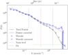 |
Fig. 4 Fourier (solid lines) and wavelet (symbols) power spectra of the NGC 2264 region. Before fitting a P(k) =A kγ relation (dashed curve), the corrected power spectra are subtracted by the noise level (plateau at the end of the original power spectrum, dotted horizontal green line) and divided by the empirical SPIRE 250 μm beam. The power spectra present two bumps, located at 1.4 and 0.1 pc (dot-dashed vertical blue lines). The intermediate scale chosento separate the three NGC 2264 subregions is indicated by a dot-dashed vertical red line. |
3.1 Splitting the NGC 2264 cloud into three subregions
In order to refine the outlines of the three NGC 2264 subregions, we performed a multiscale analysis of the NGC 2264 cloud. We used complex wavelet transforms described by Robitaille et al. (2014, 2019) to first calculate the power spectrum of the complete NGC 2264 region. While corresponding very well to the classic Fourier power spectrum, this method goes further by making it possible to visualize the spatial distribution of density fluctuations for any scale of the power spectrum. The decomposition is done with the directional and complex Morlet wavelet defined in the Fourier space as
![\begin{equation*} \begin{split} \hat{\psi}(\bm{k}) & =\textrm{e}^{-|\bm{k}-\bm{k}_0|^2/2} \\ & =\textrm{e}^{-[(u-|\bm{k}_0|\cos \theta)^2+(v-|\bm{k}_0|\sin \theta)^2]/2}, \end{split}\end{equation*}](/articles/aa/full_html/2021/01/aa39353-20/aa39353-20-eq11.png) (2)
(2)
where k = [u, v] is the wavenumber, θ is the wavelet azimuthal direction, and the constant |k0| is set to  to ensure that the admissibility condition is almost met (Kirby 2005). From this decomposition, the amount of power for the density fluctuations as a function of spatial scales is calculated following the relation
 (3)
(3)
where ⟨⟩ represents the averaging operation. The spatial scale ℓ is then converted to the Fourier wavenumber k following the relation k = |k0|∕ℓ.
Figure 4 shows the wavelet power spectrum of NGC 2264, corrected for the noise level and the 18.2′′ beam. It can be fitted by a power-law relation P(k) = A kγ (see fit parameters in Table 2), except for excess of power located at ~ 0.15 and ~ 1.5 arcmin−1 corresponding to scales of ~1.4 pc and ~0.1 pc, respectively. Figure 5 shows the spatial distribution of the power density fluctuations averaged over θ,  , for these two scales as well as the 0.47 arcmin−1 (or 0.4 pc) scale located between the two power excess. The first excess at 1.4 pc corresponds to the large-scale mass reservoir associated with the central part of the NGC 2264 cloud. This mass reservoir dominates in terms of density fluctuation at this spatial scale (see Fig. 5, left panel) as do massive hubs or ridges in, for example, the Cygnus X, Vela C, and NGC 6334 cloud complexes (Schneider et al. 2010; Hill et al. 2011; Tigé et al. 2017). This excess is also measured on NGC 2264 using the Δ-variance method (Schneider et al., in prep.). The 0.1 pc-scale image (see Fig. 5, right panel) displays smaller-scale structures associated with clumps.
The intermediate scale of 0.4 pc, which separates the scales associated with the mass reservoir of the central ridge and the mass reservoir of small-scale clumps, was chosen to refine the division of the NGC 2264 cloud into three subregions. The outline of the northern, central, and southern subregions are set to go through saddle points (see Fig. 5, middle panel). The global characteristics of these subregions observed on the Herschel column density and temperature images are listed in Table 2.
Global characteristics and cloud structure of NGC 2264 and its three subregions and fit values for the total wavelet power spectrum of NGC 2264 and for the Gaussian and coherent power spectra of the northern, southern, and central regions.
 |
Fig. 5 Power density fluctuations of NGC 2264 measured by MnGSeg and averaged over θ for three scales: 0.15 arcmin−1 (or 1.4 pc, left panel), 0.47 arcmin−1 (or 0.4 pc, middle panel), and 1.5 arcmin−1 (or 0.1 pc, right panel). Images are rotated from the RA-Dec grid (gray lines) to facilitate the wavelet decomposition. The yellow lines in the middle panel separate the three subregions of NGC 2264. |
3.2 Segmentation of the coherent and gaussian components of the cloud structure
We applied the multiscale non-Gaussian segmentation (MnGSeg) technique to investigate the hierarchical properties of the cloud structure in the three subregions of NGC 2264. This technique allows us to separate the random spatial density fluctuations of a cloud from the dense, coherent structures, usually associated with star formation activities. While we expect the Gaussian component of a cloud to only consist of evanescent structures of the interstellar medium, its coherent component contains cores, clumps, hubs, ridges, and other filamentary structures that correspond to the gas mass reservoir of present star formation. The non-Gaussian segmentation is done on wavelet coefficients as a function of orientations θ and scales ℓ (see Robitaille et al. 2019 for more details on the technique). The amount of power for the density fluctuations as a function of spatial scales,  , can be calculated according to the spatial coverage of areas of interest following the relation
 (4)
(4)
Figure 6 presents the Gaussian (random) and coherent wavelet power spectra for the three subregions of NGC 2264 and Table 2 lists the parameters of their fitted relation P(k) = A kγ + P0 for the Gaussian component and P(k) = A kγ for the coherent part. For all subregions, the coherent component dominates in terms of power over the Gaussian components. Moreover, the central subregion presents a Gaussian component which resembles, in terms of both power level and power-law index, those fitted for the northern and southern subregions. In contrast, the coherent component of the central subregion possesses a power level that is several hundred times higher than that of the northern and southern subregions. The coherent spectrum of the central subregion also displays more irregularities compared to the coherent spectra of the northern and southern parts (see Fig. 6b). We notably recover the two power excess observed in Fig. 4. As shown by Robitaille et al. (2019), the small-scale spectra flattening modeled by the variable P0 for the Gaussian components only is associated with the cosmic infrared background signal.
Recently, Robitaille et al. (2020) discussed and proved, using statistical models, that the non-Gaussian segmentation performed by MnGSeg can also be interpreted as the separation of a component of multifractal nature, the coherent part, from a monofractal component, the random Gaussian part. The multifractal nature of the coherent component means that its hierarchical structures are defined by a collection of power-law indexes rather than by a single one, as is the case for the monofractal geometry of the Gaussian component. These different fractal properties explain why the power spectra of the coherent components in Fig. 6b are more diverse and complex than those of the Gaussian components shown in Fig. 6a. It also suggests that the coherent component of a cloud (see Fig. 6b and Table 2) could reveal the complexity level of cloud structures, which increases with the creation of large gravity potentials such as hubs and ridges. A more detailed analysis of the multifractal properties of the NGC 2264 cloud, its subregions, and the local environment of clumps will be done by Robitaille et al. (in prep.).
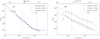 |
Fig. 6 Random Gaussian (panel a) and coherent (panel b) wavelet power spectra calculated by MnGseg for the three NGC 2264 subregions. The dotted black and red curve represents the fitted power law relations to the northern and central subregions. The coherent power spectrum of the central subregion stands out with ~ 100 times more power and bumps located at 1.4 and 0.1 pc (vertical blue dashed lines). |
4 Analysis of the population of clumps in NGC 2264
After estimating the completeness level of the catalogs of clumps identified in the three subregions of NGC 2264 (see Sect. 4.1), we characterize the main physical properties of clumps (see Sect. 4.2) and evaluate their boundedness (see Sect. 4.3). We then investigate the spatial distribution of clumps (see Sect. 4.4) and their mass segregation (see Sect. 4.5). Table 3 lists the main statistical parameters of the NGC 2264 cloud and its three subregions.
4.1 Completeness of the clump catalogs
To accurately compare the properties of the clumps between subregions, we estimated the completeness level and how it varies across the map. For this purpose, we injected a synthetic population of 1170 sources over the background image of NGC 2264, which is produced by getsf during the clump extraction process (see Sect. 2.2). Synthetic sources were split into nine bins logarithmically spaced between 0.25 M⊙ and 4.0 M⊙, with a constant number of 130 sources per bin. Their chosen density profile is that of Bonnor-Ebert spheres with a central density increasing with the clump mass, in agreement with the profile observed for clumps. These synthetic clumps, once convolved by our 18.2′′ angular resolution, display FWHM sizes of about 0.12 pc (or 35′′) corresponding to the median size of extracted sources. We ran the extraction algorithm getsf on the synthetic image with the same parameters as for the observations. In total, 695 out of 1170 (59%) sources have been recovered.
Figures A.2a,b show the detection rate of synthetic sources injected on the NGC 2264 background image. From the detection rate versus mass curve of Fig. A.2a, we estimated a global 90% completeness level of ~ 1.7 M⊙. 74 (29%) clumps of Table 1 lie above this completeness level.
The completeness level of any source extraction procedure does however depend on the intensity of the source background. We therefore computed, for each identified source, its contrast, defined as  and plot the detection rate against source contrast in Fig. A.2b. A minimum contrast of 0.4 is required to detect a source, while all sources with C > 1.7 are detected. The 90% completeness level is reached for a source contrast of C = 1.1, that is, for clumps with
  . As shown in Fig. 2 and Table 1 and 2, the background level varies strongly from the northern or southern subregions and central part of NGC 2264. We therefore used the median value of the background of the clumps to characterize each subregion:
  , 4.3 × 10²¹ and 7.3 × 1021 cm−2 in the northern, southern, and central subregions, respectively. Using the relation of mass versus peak column density found for both synthetic and observed clumps (
 , see Fig. A.3a), we computed the associated mass threshold for clumps. We obtained a 90% completeness level of ~ 1.5 M⊙ for both the northern and southern subregions and a completeness level about two times larger, 2.7 M⊙, for the central subregion of NGC 2264. As a consequence, some low-mass clumps in the center may be overlooked by the extraction algorithm. The number of clumps with masses above these 90% completeness levels are 19, 22, and 33 in the northern, southern, and central subregions, respectively.
 |
Fig. 7 Distribution of clump size (panel a) and clump mass (panel b) for the three subregions of NGC 2264: central (hatched black histograms), northern (red histograms), and southern (blue histograms) subregions. The central subregion has an excess of high-mass clumps comparedthe northern and southern subregions. The angular resolution of our observations, 18.2′′, is given in panel a. The completeness levels, ~2.7 M⊙ in the central subregion and ~1.5 M⊙ in the northern and southern subregions, are indicated in panel b with dotted lines. |
4.2 Mainphysical properties of clumps
The size and mass distributions of clumps in the northern, central, and southern subregions are presented in Figs. 7a,b. As for the clumps sizes no significant variations have been observed between subregions (see Fig. 7a). The size distributions are all centered around a median value of ~35′′, corresponding to a deconvolved size of FWHMDec ~ 0.1 pc at 723 pc. The three subregions also host a couple of clumps with FWHM sizes close to the beam, 18.2′′, and nine clumps with sizes larger than 57′′ (or 0.2 pc). At a scale of ~0.1 pc, clumps likely fragment into smaller and denser cores, which could be the main mass reservoirs of individual protostars. Such cores have been observed in the two central protoclusters, IRS1 and IRS2 by Peretto et al. (2006) and Cunningham et al. (2016).
As for the mass distribution of clumps, it strongly varies between subregions (see Fig. 7b). While they are similar in the northern and southern subregions, the mass distribution in the central subregion is strongly shifted toward higher masses. Out of the 29 clumps with masses above 4 M⊙, 24 are located in the central subregion.
4.3 Gravitational stability of clumps
In Herschel studies, the self-gravitating status of clumps is usually assessed using the Bonnor-Ebert ratio, αBE = RDec∕RBE, where RDec is the deconvolved clump radius (here FWHMdec) and RBE the radius of a critical Bonnor-Ebert sphere of the same mass, M, and same temperature, Tdust, as the source,
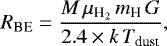 (7)
(7)
where G and k are the gravitational and Boltzman constants. This parameter estimates the ratio of the thermal support to gravitational force and clumps with αBE < 2 are considered as gravitationally bound. The Bonnor-Ebert ratio should however be considered as a rough estimator of the gravitational boundedness of the clump, since it does not include the effects of turbulence, magnetic fields, or external pressure.
Although αBE parameter theoretically depends on the mass, size, and temperature of the clump, the latter, which varies little within the sample ( K, see Fig. A.4), has little influence here. As illustrated by the mass versus size diagram shown in Fig. 8a, the separation between bound and unbound clumps appears close to horizontal in this logarithmic representation. This implies that a threshold on the Bonnor-Ebert parameter approximately corresponds to a threshold in mass, αBE < 2⇔M ≳ 1–2 M⊙. This appears more clearly on the mass distributions shown in Fig. 8b. Bound clumps are significantly more massive than unbound clumps, with a median mass of 2.6 M⊙ versus 0.5 M⊙, respectively.
In the whole NGC 2264 cloud and following the Bonnor-Ebert criterium, 36% of the clumps are gravitationally bound. In more detail, half the clumps of the central subregion are bound while they are only ~30% in the northern and southern subregions (see Table 3). This result is in line with the variation of column density background in the central subregion when compared with the southern and northern subregions (see Table 2).
Distribution of clumps and YSOs in NGC 2264 and its subregions.
 |
Fig. 8 Mass vs. size diagram (panel a) and mass distribution (panel b) for the 256 clumps detected in the NGC 2264 cloud. Gravitationally bound and unbound clumps, with αBE < 2 and αBE ≥ 2, respectively are located with red (resp. blue) markers (panel a) and sum up in a red (resp. blue) histogram (panel b). Panel a: the critical Bonnor-Ebert sphere model (αBE = 2) at the median clump temperature, Tdust = 13.9 K, is plotted asa black solid line. The physical size of the beam at a distance of 723 pc is plotted as a vertical doted line. Panel b: theglobal 90% completeness level is indicated with a doted line. |
4.4 Spatial distribution of clumps
Despite the different completeness limits of the three NGC 2264 subregions (see Sect. 4.1), clumps appear rather homogeneously distributed. There are 74, 97, and 85 clumps in the northern, central, and southern subregions, respectively (see Table 3), of which ~30% lie above their 90% completeness limit. We note, however, that the density of clumps  , defined as the ratio of the number of clumps to the subregion area, is about twice in the central subregion that in the northern and southern subregions (see Table 3).
To further investigate the spatial distribution of clumps, we first applied nearest neighbor statistics, using the distance from the center of each clump to the peak position of its nearest neighbor. The resulting distributions of nearest-neighbor clump separation are plotted in Fig. 9 for the three subregions of NGC 2264. In the northern and southern subregions, clumps have similar median distances of 0.34 pc and 0.36 pc, respectively, and cannot be statistically distinguished, according to a Kolmogorov-Smirnov (KS) test. The nearest neighbor distribution of the central subregion stands out with a large excess of clumps at short distance, ~0.1–0.2 pc, and a median clump separation of ~0.22 pc, which is 1.6times lower than in the northern and southern subregions. A KS test rejects, with a p-value below 10−4, the hypothesis that the central and northern + southern subregions might have a common distance distribution. Interestingly, the clumps at the center of NGC 2264 are closely packed, with separations of about twice their median FWHM size, ~0.11 pc (see Sect. 4.2), and thus once their outer diameter. These clumps are mostly located in the two IRS1 and IRS2 protoclusters of NGC 2264 (see Fig. 3).
We also computed the Q parameter (Cartwright & Whitworth 2004) for the NGC 2264 cloud and its three subregions (see Table 3). The Q parameter method is based on the minimum spanning tree (MST), which is the set of straight lines (the edges) connecting a given set of points(here the center of the clumps) without closed loops, such that the sum of all edges lengths is minimal. The Q parameter is defined as the ratio of the normalized mean edge length calculated by the MST,  , to the mean clump separation,
  :
:
 (8)
(8)
The Q values above 0.8 are associated with centrally concentrated spatial distribution, while lower Q values indicate subclustering. With Q ≃ 0.7, the NGC 2264 cloud overall displays only a moderate amount of subclustering for its clump population. Locally, the southern subregion appears to be more subclustered compared to the central and northern subregions (Q ≃ 0.6 versus Q ≃ 0.8). On the column density map (see Fig. 2), we observed that its clumps are distributed either in a north-south filament joining the central subregion or in the southwestern part of NGC 2264.
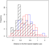 |
Fig. 9 Distribution of the distance to the first nearest neighbor for clumps in the central (black hatched histogram), northern (red histogram), and southern (blue histogram) subregions of NGC 2264. Clumps are 1.6 times more closely packed in the central subregion than in the two others. |
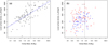 |
Fig. 10 Local surface density Σ6 as a function of the mass of the clump for the central subregion of NGC 2264 (panel a, black markers) and in the northern and southern subregions (panel b, red and blue markers, respectively). The potential correlation between Σ6 and M in a, Σ6∝ M0.47 is represented by a dashed blue line in both panels a and b. Completeness levels are indicated by dotted vertical lines. |
4.5 Mass segregation of clumps
Mass segregation refers to a difference between the spatial distribution of massive objects compared to that of their lower-mass counterparts. The methods used to quantify mass segregation have evolved with our current view on the subject and are associated with slightly different definitions, but in general, all of these methods compare the distribution of high- and low-mass stars. Amongst them, the local surface density Σj (Maschberger & Clarke 2011), and mass segregation ratio ΛMSR (Allison et al. 2009) do not require a specific definition of a cluster center and are the most widely used. They most probably also give the most robust results when combined (e.g., Parker & Goodwin 2015). We applied both methods to measure the mass segregation of clumps in NGC 2264 and its subregions, again using the peak position of the clumps as a reference. The impact of the clumps spatial extent in these statistics will be investigated in future studies (Thomasson et al., in prep.).
The first method calculates the local surface density of source, Σj, within an area encompassing the jth nearest neighbor, at a distance of rj as follows:
 (9)
(9)
As proposed by Maschberger & Clarke (2011), we took j = 6, as it constitutes a good compromise between estimating the local density and reducing low-number fluctuations (see also Casertano & Hut 1985).
Figures 10a,b present the Σ6 versus M diagrams that investigate if high-mass clumps are in denser groups than their lower-mass counterparts. Since the clump populations of the northern and southern subregions exhibited similar behaviors in Sects. 4.2–4.4, we assembled their clump samples. In contrast, we kept the central subregion alone since its clump sample had rather different characteristics. In the central subregion, the local surface density correlates with the mass of the clumps, with a Pearson correlation coefficient of 0.75 (see Fig. 10a). However, when accounting for the 90% completeness level of 2.7 M⊙ (see Sect. 4.1), we cannot exclude low-mass clumps in high-density groups have not been detected. Therefore, the most robust result of this Σ6 analysis is that high-mass clumps in the central subregions are only found in high-density groups. The 15 most massive, >9.3 M⊙, clumps in NGC 2264, closely packed in the IRS1 and IRS2 protoclusters (see Fig. 3 and Sect. 4.4), have a median Σ6 density about three times that of all clumps in NGC 2264 center. Conversely, the lower-mass clumps in the northern and southern subregions do not present a privileged location in high- or low-density groups according to their mass (see Fig. 10b).
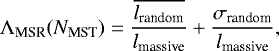
The second method to quantify mass segregation compares the MST of the most massive objects (here clumps) of a sample with the MST of randoms subsets of objects in this sample (see Allison et al. 2009). The mass segregation ratio, ΛMSR, is calculated as
 (10)
(10)
where lmassive is the length of MST for the NMST most massive clumps and  is the average length of MST for NMST random clumps. It was computed for 500 sets of NMST random clumps along with the associated standard deviation, σrandom. A value of ΛMSR ≈ 1 indicates that the spatial distribution of massive clumps is comparable to that of other clumps and therefore that there is no mass segregation. Higher ΛMSR values suggest that massive clumps are more concentrated than their lower-mass counterparts.
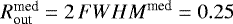
Figures 11a,b show ΛMSR, for an increasing number, NMST, of the most massive clumps for the NGC 2264 cloud and its subregions. The clump population of NGC 2264 appears to be strongly mass segregated, with values of ΛMSR around 7.8 for NMST ≤ 15. If we consider only the central subregion, which contains the most massive clumps, segregation is still present, but the ΛMSR value decreases to ~3.7. This decrease is explained by lower lrandom values for clumps distributed in the central subregion than over the whole NGC 2264 cloud. In Fig. 11a, ΛMSR drops to 4 for NMST = 16, because the 16th most massive clump is the first located outside the IRS1 and IRS2 protoclusters. Mass segregation remains significant, with ΛMSR values above 1 with more than 2 sigma uncertainty, up to NMST ≃ 30. In contrast, for the clump samples of the northern and southern subregions, Fig. 11b do not reveal any mass segregation. The ΛMSR plateau observed are listed in Table 3.
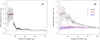 |
Fig. 11 Masssegregation ratio, ΛMSR, as a functionof the numbers of clumps, NMST, in the NGC 2264 cloud (panel a) and in its three subregions (panel b). Error bars represent the ± 2σ uncertainties. Values above ΛMSR ≃ 1 (black solid line) suggest mass segregation. Completeness levels are indicated with vertical dashed lines. Panel a: median segregation ratio for the 15 most massive clumps of NGC 2264, calculated over NMST= 4 to 15, is |

5 Combined analysis of the YSO and clump populations in NGC 2264
In this section, we analyze the YSO content of the NGC 2264 subregions (Sect. 5.1) and quantify the link between the YSO and clump populations (Sect. 5.2).
5.1 Distribution in the NGC 2264 subregions
The spatial distribution of the clump and YSO populations is illustrated in Fig. 12. The clump population is rather homogeneously distributed over the whole Herschel area (see Sect. 4.4) even if it obviously follows the gas concentration toward the two IRS1 and IRS2 protoclusters and the Y-shaped filament. The YSOs themselves cluster in three places: strongly around the IRS1 and IRS2 protoclusters and more distributed around the S Mon massive star.
Table 3 lists the number of YSOs regardless of their class, the number of Class 0/I protostars, and Class II pre-main sequence stars found by Rapson et al. (2014) in NGC 2264. We distributed this YSO population among the three subregions of the NGC 2264 cloud defined in Sect. 3.1. Unlike the spatial distribution of clumps in subregions, a very uneven distribution is observed for the YSOs. The central subregion, which accounts for 22% of the whole NGC 2264 cloud area and contains 38% of the detected clumps (see Tables 2, 3) gathers up to 62% (302 out of 485) of the YSO population. In contrast, the southern subregion, which covers 45% of the whole cloud, contains 33% of the clumps but only 6% (27 out of 485) of the YSOs. This clear lack of YSOs in this subregion cannot be explained by the small area of the Herschel image not investigated for YSOs by Rapson et al. (2014) (see Fig. 12). The northern subregion shows a more balanced distribution with 33, 29, and 32% of the cloud area, clump, and YSO populations.
Regarding the evolutionary class of YSOs, the northern subregion is almost exclusively populated by Class II sources (146 out of 156, 95%, see Table 3). On the other hand, the distribution is more balanced in the central and southern subregions: 23–30% of the YSOs are Class 0/I protostars and the complementary 70–77% are Class II sources. Finally, we found that the 69 Class 0/I in the central subregion represent a large majority (79%, see Table 3) of this younger YSO population in the whole NGC 2264 cloud.
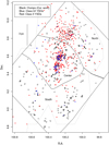 |
Fig. 12 Spatial distribution of the clump (black ellipses) and YSO populations in the NGC 2264 cloud, as taken from the catalogs of Table 1 and Rapson et al. (2014). Bound clumps are represented with filled ellipses. Class 0/I (blue star markers) and Class II (red star markers) sources were identified in the area outlined by dotted black lines. The three subregions of NGC 2264 (see Sect. 3.1) are outlined and labeled in black. Clumps are much more homogeneously distributed over the NGC 2264 cloud than YSOs. |
5.2 Link between the clump and YSO populations
We investigated the spatial correlation between the clump and YSO populations found in the different subregions of NGC 2264 using the nearest neighbor statistics. Figures 13a–d show the distributions of the distance to the first nearest neighbor (nnd) from YSOs to clumps and vice versa, with YSO populations separated into Class 0/I protostars and Class II pre-main sequence stars. Class-0/I and clumps are similarly distributed in the northern and southern subregions (see Table 3 and Fig. 12); in addition the nnd distributions between Class-0/I and clumps cannot be statistically distinguished, according to a KS test. We therefore combined the northern and southern populations of Class 0/I protostars to increase the sample size (18 objects). The ten clumps detected in the Herschel area not covered by Spitzer (see Fig. 12 and Table 3), and thus not surveyed for YSOs by Rapson et al. (2014), were excluded from our analysis.
The nearest neighbor distance, nnd, distribution between Class 0/I protostars and clumps first illustrates the strong link between Class 0/I protostars and their parental clump. The large majority (80−95%) of the Class 0s/Is of each of the NGC 2264 subregions lie at a distance smaller than the median outer radius of clumps (i.e., below 0.25 pc; see Fig. 13a). Conversely, the nnd distribution of clumps with respect to Class 0/I protostars shows in Fig. 13b that ~40% of the clumps in the central subregion host, within their outer radius, at least one Class 0/I protostar. This fraction increases to two-thirds when considering only bound clumps in the central subregion. In addition to illustrating this parental link, the nnd distributions between clumps and Class 0s/Is presents, for both the central and northern + southern samples, a peak around 1 pc (see Fig. 13b). This peak shows that aside the population of clumps tightly linked to Class 0/I, mostly clustered in the central region, there exists a disperse population of clumps that are not associated with Class 0/I YSOs all over NGC 2264. As a matter of fact, most of the clumps that create this peak, that is, ~75% no matter which subregion, are qualified as unbound. These unbound clumps could be more than transient cloud fragments because the external gas pressure associated with the global collapse is not taken into account in the calculation of gravitational boundedness. Excluding clumps presently qualified as unbound however, the nnd distribution between clumps and Class 0s/Is still displays a peak, which is weaker and located at ~0.5 pc.
Figures 13c,d show the nnd distributions between clumps and Class II pre-main sequence stars. Given the proper motions found by Buckner et al. (2020) for the weakly embedded Class II sources in the NGC 2264 cloud, ~1 mas yr−1, and their estimated age, ~×106 yr found by Venuti et al. (2018), these sources could have dispersed by ~6 pc from their original birth site. For these Class II sources, we thus do not expect a direct parental link between Class IIs and the presently observed clumps. Other Class II pre-main sequence stars could remain more tightly associated with their birth site, as is probably the case in the NGC 2264 IRS1 and IRS2 protoclusters. The histograms of Figs. 13c,d should thus reveal the parental link of a clustered population of Class IIs plus the average spatial distributions of a more extended population of Class IIs, with no direct parental link with clumps. If the small number, 19, of Class II YSOs in the southern subregion makes any detailed characterization of the histogram shown in Fig. 13c not relevant, that of Fig. 13d should be robust to interpret. While the nnd distributions between clumps and Class II sources are similar in the central and northern subregions, the distribution in the southern subregion clearly stands out as different (see Fig. 13d). The former are both broadly distributed around ~0.2 pc.
In contrast, in the southern subregion, the nnd distribution between clumps and Class IIs presents a strong peak at ~1 pc, which means at much further distances than in the other parts of the cloud. This definitively is a consequence of the low density of YSOs observed in the southern subregion (see Fig. 12). We can question the association of Class IIs with the southern subregion or even their membership in the NGC 2264 cloud. Indeed, with proper motions such as those measured by Buckner et al. (2020), the Class IIs observed in the southern subregion could have formed in, and been ejected from, the central subregion of NGC 2264. As a guideline, Buckner et al. (2020) also estimated that up to 30% of the YSOs observed in the area covered by the NGC 2264 cloud may not be members of this star-forming region. A detailed comparison of the star and cloud velocities measured with ground-based radiotelescopes and the Gaia observatory would be necessary to evaluate the YSO membership in the southern subregion of NGC 2264.
The comparison of the nnd distributions of clumps with respect to YSOs (see Figs. 13b and d), in the central and northern subregions, leads to an apparent counterintuitive result. On average, clumps are closer to Class II pre-main sequence stars than to Class 0/I protostars: median nnd of 0.2 pc versus ≃0.8 pc. This reflectsthe differences in the spatial distribution visible in Fig. 12. While the large majority of Class 0s/Is are clustered in the IRS1 and IRS2 protoclusters, Class IIs and clumps display a more distributed population. This is totally inconsistent with scenarios of quiet cloud formation followed by a continuous process of star formation (see, e.g., Shu et al. 1987; Krumholz 2014).
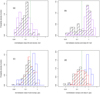 |
Fig. 13 Distribution of the distance to the first nearest neighbor, nnd, from YSOs to clumps (panels a and c) and from clumps to YSOs (panels b and d). The YSOs are Class 0/I in the upper panels (a and b), Class II in the lower panels (c and d). Distributions are presented for the central subregion (hatched black histograms) and for the northern and southern subregions, combined in the upper panel (purple histogram) and separated in the lower panel (red and blue histograms, respectively). Distributions are normalized to facilitate the comparison involving small populations of YSOs (Class 0/I from northern and southern subregions in panel a, Class II from southern subregions in panel c). The dashedvertical red line indicates the median outer radius of clumps, calculated as twice the median FWHM: |
6 Discussion
We hereafter make the link between evidence for mass segregation observed for NGC 2264 clumps and the cloud structure (see Sect. 6.1) and propose an updated scenario for the star and thus cloud formation history in NGC 2264 (see Sect. 6.2).
6.1 Masssegregation of clumps and its relationship to cloud structure
Mass segregation has been studied extensively in stellar clusters for decades. More recently, mass segregation has been investigated for cloud fragments with 0.002 pc to 0.1 pc sizes, using tools developed for stellar clusters. In particular, Dib & Henning (2019) calculated the mass segregation ratio of cores in four star-forming regions: Taurus, Aquila, Corona Australis, and W43-MM1. These authors found no mass segregation in Taurus but a significant level of mass segregation in the three other clouds: ΛMSR up to 4–9 for the 6–14 most massive cores. Plunkett et al. (2018) also reported that Serpens South is mass segregated, with a median ΛMSR ≃ 4 for the NMST ≤ 18 most massive cores. Parker (2018) and Könyves et al. (2020) in Orion B, Román-Zúñiga et al. (2019) in Orion A, and Sadaghiani et al. (2020) in NGC 6334 also claimed to find mass segregation, although with lower values (ΛMSR ≃ 2−3) and/or involving a smaller number of cores. Besides, no significant mass segregation was found in 12 infrared-dark clouds by Sanhueza et al. (2019). As for the surface density parameter, Σj, sometimes used to quantify mass segregation, it was up to now only computed for a couple of star-forming regions. Lane et al. (2016), Parker (2018), and Dib & Henning (2019) notably reported tentative trends for the most massive cores in Orion-A, Orion B, and Corona Australis to sit in areas of higher local surface density. In particular, Lane et al. (2016) found in Orion B a median Σ10 value two times larger for the ten most massive cores than for the whole source samples.
The mass segregation found in NGC 2264 (see Sect. 4.5) is among the strongest and affects the largest numbers of objects when compared to these published results. The ΛMSR parameter is measured to be ΛMSR ≃ 8 for the NMST = 4–15 most massive clumps (see Table 3 and Fig. 11a). Moreover, mass segregation remains significant for the ~30 most massive clumps of the NGC 2264 cloud. When the mass segregation is measured by the local surface density, it has a median Σ6 value for the 15 most massive clumps four times higher than that of the whole sample. We refrained from making more quantitative comparisons with published studies since the ΛMSR values are measured with different methods (e.g., the sliding window in Román-Zúñiga et al. 2019; Könyves et al. 2020 instead of the cumulative form in this work) and the datasets are inhomogeneous. Sources were extracted with different extraction tools (e.g., clumpfind in Román-Zúñiga et al. 2019, FellWalker in Parker 2018 vs. getsf in this work) and thus have various definitions. The cloud fragments considered also have different physical sizes, which range from ~0.002 pc (or ~400 AU) in Plunkett et al. (2018), 0.01–0.03 pc (or 2000–6000 AU) in Dib & Henning (2019), to ~0.1 pc (or ~2 × 10⁴ AU) in the present study. Moreover, there are also issues, generally not taken into account, related to the incompleteness of samples and crowding of sources in measuring the mass segregation in dense environments such as massive (proto)clusters (Ascenso et al. 2009).
As shown in Fig. 11b, this strong mass segregation is entirely due to the concentration of high-mass clumps in the NGC 2264-IRS1 and IRS2 protoclusters in the central subregion. We showed that these high-mass clumps all are gravitationally bound and lie at short distance from each other (see Sects. 4.3 and 4.4 and Fig. 3), thus forming a cluster of star-forming clumps. The overabundance of high-mass clumps in the central subregion of NGC 2264 relative to the northern and southern subregions is consistent with its greater gas concentration. After removing clumps from the column density image of Fig. 2, the average column density of this background, at the location of clumps, is almost twice as high in the central subregion as in the other NGC 2264 subregions (see Table 2). The relation between themass of cloud fragments and their surrounding gas has been reported for several star-forming regions (e.g., Könyves et al. 2020) and in this work presents a linear correlation between the mass of NGC 2264 clumps, M, and the column density of their surrounding background,  (see Fig. A.5). The incompleteness level of the clump sample could however partly explain this linear correlation and especially the lack of low-mass clumps over regions with high background level.
The overabundance of high-mass clumps in the central subregion is also in line with the fact that its hierarchical structure is different from that of the northern and southern subregions (see Sect. 3.2). The power spectrum of the central subregion, which is hundred times stronger, consists of the sum of a power-law function plus power excesses at the scales of cloud and clump mass reservoirs (see Fig. 6b and Table 2). While diffuse clouds and Gould Belt clouds generally have simple multifractal power spectra (Robitaille et al. 2019, 2020), those of high-mass star-forming regions are more complex and dominated, at given scales, by large gravity potentials such as hubs and ridges (Robitaille et al., in prep.). Following the definition criteria set in HOBYS articles (e.g., Hill et al. 2011; Hennemann et al. 2012; Nguyen Luong et al. 2013) and precursor papers (Schneider et al. 2010), the central part of the central subregion of NGC 2264 qualifies as a ridge. In short, ridges are very dense, >105 cm−3, ~1 pc cloud structures actively forming clusters of intermediate- to high-mass stars (Motte et al. 2018). The center of NGC 2264 hosts a dense north-south filament, which appears as a privileged site for intermediate- to high-mass star formation (see Figs. 3 and 12). It contains a cluster of massive clumps hosting protostars, which could ultimately form a rich YSO cluster with at least a handful of high-mass stars. The mass segregation observed for the NGC 2264 clumps could thus be at the origin of the mass segregation of future stars in, at least, the central stellar cluster of NGC 2264.
We postulate that this mass segregation could come from further afield, in the very way the mass of gas was assembled to form the molecular cloud in the NGC 2264 region. The large-scale kinematics observed throughout the Monoceros cloud complex (Loren 1977; Montillaud et al. 2019) and the global infall discovered toward the NGC 2264-IRS1 protocluster (Williams & Garland 2002; Peretto et al. 2006) suggest that a hierarchical collapse of the NGC 2264 cloud could have led to the formation of a ridge at its center. Further studies of the cloud kinematics are necessary to investigate whether the three filaments that appear converging toward the central ridge drive material and therefore feed the ridge and its protoclusters. This mode of cloud and thus star formation by competitive, inflowing gas is advocated in theories of hierarchical global collapse (e.g., Vázquez-Semadeni et al. 2019), gravitationally-driven gas inflows (e.g., Smith et al. 2009; Hartmann et al. 2012), filament or conveyor-belt collapse (Myers 2009; Krumholz & McKee 2020), and colliding flows (e.g., Heitsch et al. 2008).
6.2 Star formation history in NGC 2264
Evidence for sequential star formation in NGC 2264 has been presented by several YSO studies (Sung & Bessell 2010; Teixeira et al. 2012; Rapson et al. 2014; Venuti et al. 2018). Venuti et al. (2018) proposed that star formation began ~5 Myr ago in the northern subregion and, more precisely, in the S Mon area. Then, less than 1 Myr ago, star formation could have developed in the central subregion and especially in the NGC 2264-IRS1 and IRS2 protoclusters. In the present study, this age gradient is qualitatively confirmed when comparing YSO distributions of the northern and central subregions. The central subregion concentrates about 80% of the total Class 0/I protostars of the NGC 2264 cloud, while the northern subregion is mainly populated by Class II pre-main sequence stars (see Table 3 and Sect. 5.1). As for the southern subregion of the NGC 2264, it has not been considered in YSO studies because it contains very few YSOs, only 6% of the total population, suggesting that star formation has not yet been active there. To more accurately compare subregions, Fig. 14 shows, for each YSO (Class II and Class 0/I) population, their surface density divided by their statistical lifetime. Surface densities, Σobject, are calculated using the number of objects in each YSO class and the subregion surfaces listed in Tables 2 and 3. We assumed lifetimes, τobject, of 2 × 10⁵ and 2 × 10⁶ yr for Class I protostars and Class II pre-main sequence stars, respectively, in agreement with Evans et al. (2009) and Venuti et al. (2018) and references therein. Error bars on Σobject∕τobject take into account statistical uncertainties, as well as an estimation of potentially undetected Class 0/Is in the central region and field contamination of Class II population (see Sect. 5.2 and Buckner et al. 2020). The surface densities per lifetime of Class IIs and Class 0/Is are similar in the northern subregion. This behavior is consistent with the idea that a continuous star formation activity has developed in the northern part of NGC 2264 over the past few 106 yr. In contrast, in the central and southern subregions, the surface densities per lifetime are three to five times higher for Class 0/I protostars than those measured for Class IIs, suggesting an increase of the star formation activity over the past few 105 yr.
Identifying and characterizing the ~0.1 pc clumps in NGC 2264, using its Herschel column density image, for the first time, allows us to study the gas mass reservoir for current and future star formation in the NGC 2264 cloud. In particular, bound clumps represent structures that are forming or are likely to form stars in the near future. The clump lifetime is not as properly defined as the one of YSOs but, with a median density of ~ 8 × 103 cm−3, they could live for one free-fall time (i.e., ~3 × 10⁵ yr). With the goal to further characterize the relative star formation activity in the NGC 2264 cloud, Fig. 14 shows the surface density per lifetime of bound clumps, as measured in the three subregions of NGC 2264. We estimate that the Σclump∕τclump values are uncertain by a factor of at least two. As the median densities of clumps vary by a factor of 2 depending on the subregions, the clump free-fall time is thus uncertain by a factor of ~ 50 %. Other sources of uncertainty are the number of protostars that form in each clump, taken as one, and the number of free-fall times, assumed to be one, required for these clumps to form stars. With our current assumptions, the surface density per lifetime of clumps is similar to that of YSOs in the northern subregion, implying a continuous star formation activity. In contrast in the southern subregion, Fig. 14 suggests a tentative increase of the surface density per lifetime of clumps compared to that of the YSOs and therefore a possible increase of the star formation activity from 106 years ago to the next few 105 years. In the central subregion, uncertainties are too large to conclude that there is any trend for future star formation activity relative to the current star formation activity. All in one, the spatial distribution of YSO and clump populations suggests that the star formation activity will get more and more intense as we go through the NGC 2264 cloud, from north to south, in the coming ~ 3 × 10⁵ yr. Star formation first developed mainly in the northern subregion and continues today. Star formation is now extremely active in the central subregion, while it was less so in the past. Star formation now begins in the southern subregion and could get more active while it was almost nonexistent in the past. This time sequence, based on the study of clump and YSO populations, agrees and extends the evolutionary sequence proposed by, for example, Venuti et al. (2018).
We propose that this sequence of star formation is related to a prior sequence of cloud formation, first in the north, now in the center, and in the future in the south of NGC 2264. With its large mass reservoir at pc scale (see Table 2), the central subregion, and especially its ridge, has a very large potential for new events of star formation. The cloud power spectrum of the central subregion, and especially its coherent component associated with star formation, also implies that the cloud reservoir for star formation will remain important or will even increase in the coming 106 yr (see Fig. 6b). Indeed, the coherent component of the cloud contains almost all the power and thus most of the gas mass reservoir in the central subregion (see Figs. 6a,b, Fig. 14 and Table 2). Interestingly, this fraction of coherent cloud structures supposedly associated with star formation is orders of magnitude larger in the central subregion of NGC 2264 than in the northern and southern subregions. The southern subregion has similar properties with respect to its gas distribution (column density and power spectrum) than the northern subregion (see Fig. 6b and Table 3). These observations of the gas thus show that the northern and southern subregions should have the same potential for future star formation events, that is, a similar numbers of stars that could form in the coming ~ 106 yr. This is also consistent with the similarity observed in term of mass, boundedness, and surface density (see Fig. 14 and Table. 3). We therefore propose that the NGC 2264 cloud initially concentrated in the northern region several Myrs ago. The cloud distribution in the central subregion makes a strong case for extremely active cloud formation activity now and possibly in the coming 106 yr. As for the southern subregion, cloud is not yet highly concentrated but it could be enhanced in the close future. Kinematical studies of the NGC 2264 cloud are obviously necessary to confirm this last assertion.
Over the past few Myr, the NGC 2264 cloud has thus undergone several episodes of cloud and thus star formation. We showed in Sect. 5.2 that a large fraction of clumps in the NGC 2264-IRS1 and IRS2 protoclusters are the parental cloud structures from which the Class 0/I protostars currently gather their mass. In addition, a population of clumps is observed at large, ~1 pc, distances from the current sites of star formation activity (see Figs. 12 and 13b). These clumps are smaller in mass and mostly unbound. They thus need to gather more mass and concentrate themselves before they could be considered as cloud structures that will form new protostars. Future star formation episodes could develop either next to the current star formation sites or clumps must first be driven toward them. The population of clumps also appears to be spatially well correlated with Class II pre-main sequence stars, surprisingly better than with Class 0/I protostars. These elements argue for a dynamical scenario of star formation in NGC 2264. We speculate that, first and simultaneously, the cloud undergoes global collapse and clumps converge toward the central gravity potentials, called ridges, reducing their distance to star-forming sites. Protostellar collapse would then form a cluster of stars with a definite mass segregation at birth. The last phase would then be, for at least part of the population of pre-main sequence stars, to disperse from their original birth sites and spread over the entire extent of the NGC 2264 cloud, thus simulating a tight spatial correlation with a new generation of clumps. Whether the most massive and most clustered protostars, embedded within cloud ridgeswill become closely packed main-sequence stars will define whether mass segregation is determined at birth in NGC 2264 and potentially in other dynamical clouds. This scenario is consistent with the finding of Buckner et al. (2020) that YSOs with increasing evolutionary stages tend to be less clustered. It would also qualitatively agree with numerical simulations of cloud formation through, for example, the hierarchical global collapse (Vázquez-Semadeni et al. 2019) and stellar cluster evolution with the ejection of many YSOs members (Oh & Kroupa 2016).
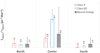 |
Fig. 14 Surface density per lifetime, Σobject∕τobject, of Class II YSOs, Class 0/I protostars, and clumps in the three NGC 2264 subregions. Statistical lifetimes of 2, 0.2, and 0.3 Myr were assumed for Class IIs, Class 0/Is, and clumps, respectively. Error bars take into account statistical uncertainties, contamination level of 30% for Class IIs, an incompleteness level of 25% for the Class 0/I population in the central subregion, and a factor of two of uncertainty for the clumps. While the star formation activity of the northern subregion appears to be constant, it displays a burst in the central subregion and shows a tentative increase in the southern subregion. |
7 Conclusions
We used a Herschel column density image of the NGC 2264 cloud to identify and characterize its clumps, study their spatial distribution, and make the link of these clumps with the YSO population and cloud structure. Our main results can be summarized as follows:
- 1.
We applied getsf to the 18.2′′ angular resolution column density image. We found a population of 256 clumps with ~0.1 pc sizes, ~14 K temperature, and masses ranging from 0.08 M⊙ to 53 M⊙. Of the NGC 2264 clumps, 36% are gravitationally bound following the Bonnor-Ebert criterium.
- 2.
After analyzing the cloud structure, we divided the NGC 2264 cloud into three subregions (northern, central, and southern) of roughly similar areas. The MnGseg technique revealed that the coherent cloud component associated with star formation dominates over the Gaussian component, especially for the central subregion. We qualified the cloud structure at the center of the central subregion of NGC 2264 as a ridge because it is massive and hosts the NGC 2264-IRS1 and IRS2 protoclusters.
- 3.
We then applied the nnd statistics to characterize the spatial distribution of clumps in the NGC 2264 cloud. The majority of the clumps are low-mass, unbound structures distributed all over the cloud. In addition, we found within the NGC 2264 ridge a cluster of higher-mass, bound clumps. The typical distance between clumps in this second population is half that found elsewhere.
- 4.
We quantified the mass segregation of NGC 2264 clumps using two complementary methods. The 15 most massive clumps, which have M = 9.3−53 M⊙ and are all located in the central protoclusters, have a median local surface density, Σ6, three times that of the entire clump population. This high degree of mass segregation is also indicated by the strong mass segregation ratio: ΛMSR ≃ 8 for the NMST ≤ 15 most massive clumps. We propose that this mass segregation is due to the presence and therefore the formation of a ridge by the global collapse of clouds in the central subregion of NGC 2264.
- 5.
Except for those in the ridge, most of the clumps in the NGC 2264 cloud are not associated with Class 0/I protostars. At odds with what a parental link would suggest, nnd distributions notably show that the spatial distribution of clumps better correlates with that of Class II pre-main sequence stars. This argues for a dynamical scenario in which clumps are driven to the central parts of the NGC 2264, protostars are formed in situ, and some Class IIs are ejected from their birth site.
- 6.
Our combined study of clump and YSO populations in NGC 2264 agrees and extends the sequential star formation sequence from north to south, which was initially proposed by YSO studies. Star formation first developed in the northern subregion. It is now extremely active in the central subregion and should soon begin in the southern subregion. We propose to explain this by a sequence of cloud formation from north to south.
The strong mass segregation observed for the NGC 2264 clumps, which is most likely due to the formation of a favorable cloud structure, the ridge, could itself be at the origin of future mass segregation in the NGC 2264 stellar cluster. Detailed studies of the cloud and YSO kinematics are mandatory to confirm our current interpretation and predictions.
Acknowledgements
This project has received funding from the European Union’s Horizon 2020 research and innovation programs StarFormMapper under grant agreement No 687528 and Filaments-to-stars under the Marie Skłodowska-Curie Grant Agreement No. 750920. This project was also supported by the Programme National de Physique Stellaire and Physique et Chimie du Milieu Interstellaire (PNPS and PCMI) of CNRS/INSU (with INC/INP/IN2P3) co-funded by CEA and CNES. This research has made use of data from the Herschel imaging survey of OB young stellar objects (HOBYS) project (http://hobys-herschel. cea.fr). HOBYS is a Herschel Key Program jointly carried out by SPIRE Specialist Astronomy Group 3 (SAG 3), scientists of several institutes in the PACS Consortium (LAM Marseille and CEA Saclay), and scientists of the Herschel Science Center (HSC).
Appendix A Additional figures
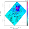 |
Fig. A.1 Herschel dust temperature image of the NGC 2264 cloud, with 3.4 × 10²¹ H2 cm−2 and 1.6 × 10²² H2 cm−2 contours taken from the column density image of Fig. 2. The resolution of the map, 18.2′′, is shown in the lower right corner and a scale bar is given in the upper left corner. A white star locates the OB star cluster, which heats its surrounding cloud over several parsecs. The IRS1 and IRS2 protoclusters are also indicated. |
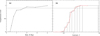 |
Fig. A.2 Completeness level of the clumps extraction as a function of the clump mass (panel a) and of the contrast of the clump column density over its local background (panel b). The 90% completeness level is indicated with a dashed horizontal line. Panel a: the clump sample is 90% complete above 1.7 M⊙. Panel b: thehistogram has been constructed with a constant number of 80 synthetic sources in the 11 first bins, plus a bin containing the remaining 290 sources that have all been detected. The red curve connects the median contrast value in each bin. Of the clumps, 90% are detected for a contrast larger than 1.1. |
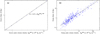 |
Fig. A.3 Mass as a function of peak column density for synthetic sources (panel a) and for observed clumps (panel b). A simple regression gives the relation |
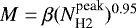
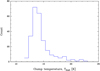 |
Fig. A.4 Temperature distribution of the 256 clumps detected in NGC 2264. The temperature dispersion between clumps is small, 80% of the clumps having a temperature between 12.7 and 16.9 K |
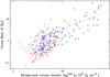 |
Fig. A.5 Correlation observed between the clump mass and its background column density. The color code highlighting the spatial location of the clumps is the same as in Fig. 7. The completeness curve in dotted line is calculated using a 90% completeness contrast of 1.1 and the M- |

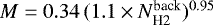
References
- Allison, R. J., Goodwin, S. P., Parker, R. J., et al. 2009, MNRAS, 395, 1449 [Google Scholar]
- André, P., Men’shchikov, A., Bontemps, S., et al. 2010, A&A, 518, L102 [NASA ADS] [CrossRef] [EDP Sciences] [Google Scholar]
- Ascenso, J., Alves, J., & Lago, M. T. V. T. 2009, A&A, 495, 147 [NASA ADS] [CrossRef] [EDP Sciences] [Google Scholar]
- Buckner, A. S. M., Khorrami, Z., González, M., et al. 2020, A&A, 636, A80 [NASA ADS] [CrossRef] [EDP Sciences] [Google Scholar]
- Cantat-Gaudin, T., Jordi, C., Vallenari, A., et al. 2018, A&A, 618, A93 [NASA ADS] [CrossRef] [EDP Sciences] [Google Scholar]
- Cartwright, A., & Whitworth, A. P. 2004, MNRAS, 348, 589 [NASA ADS] [CrossRef] [Google Scholar]
- Casertano, S., & Hut, P. 1985, ApJ, 298, 80 [Google Scholar]
- Cody, A. M., Stauffer, J., Baglin, A., et al. 2014, AJ, 147, 82 [NASA ADS] [CrossRef] [Google Scholar]
- Cunningham, N., Lumsden, S. L., Cyganowski, C. J., Maud, L. T., & Purcell, C. 2016, MNRAS, 458, 1742 [NASA ADS] [CrossRef] [Google Scholar]
- Dahm, S. E. 2008, Handbook of Star Forming Regions, ed. B. Reipurth (San Francisco: ASP), 4, 966 [NASA ADS] [Google Scholar]
- Dib, S., & Henning, T. 2019, A&A, 629, A135 [NASA ADS] [CrossRef] [EDP Sciences] [Google Scholar]
- Dib, S., Schmeja, S., & Parker, R. J. 2018, MNRAS, 473, 849 [NASA ADS] [CrossRef] [EDP Sciences] [Google Scholar]
- Didelon, P., Motte, F., Tremblin, P., et al. 2015, A&A, 584, A4 [NASA ADS] [CrossRef] [EDP Sciences] [Google Scholar]
- Evans, Neal J. I., Dunham, M. M., Jørgensen, J. K., et al. 2009, ApJS, 181, 321 [NASA ADS] [CrossRef] [Google Scholar]
- Fujii, M. S., & Portegies Zwart S. 2016, ApJ, 817, 4 [NASA ADS] [CrossRef] [Google Scholar]
- Griffin, M. J., Abergel, A., Abreu, A., et al. 2010, A&A, 518, L3 [EDP Sciences] [Google Scholar]
- Gutermuth, R. A., Megeath, S. T., Myers, P. C., et al. 2009, ApJS, 184, 18 [NASA ADS] [CrossRef] [Google Scholar]
- Hartmann, L., Ballesteros-Paredes, J., & Heitsch, F. 2012, MNRAS, 420, 1457 [Google Scholar]
- Heitsch, F., Hartmann, L. W., Slyz, A. D., Devriendt, J. E. G., & Burkert, A. 2008, ApJ, 674, 316 [NASA ADS] [CrossRef] [Google Scholar]
- Hennemann, M., Motte, F., Schneider, N., et al. 2012, A&A, 543, L3 [NASA ADS] [CrossRef] [EDP Sciences] [Google Scholar]
- Hetem, A., & Gregorio-Hetem, J. 2019, MNRAS, 490, 2521 [Google Scholar]
- Hill, T., Motte, F., Didelon, P., et al. 2011, A&A, 533, A94 [NASA ADS] [CrossRef] [EDP Sciences] [Google Scholar]
- Hill, T., Motte, F., Didelon, P., et al. 2012, A&A, 542, A114 [NASA ADS] [CrossRef] [EDP Sciences] [Google Scholar]
- Juvela, M., Ristorcelli, I., Pagani, L., et al. 2012, A&A, 541, A12 [NASA ADS] [CrossRef] [EDP Sciences] [Google Scholar]
- Kirby, J. F. 2005, Comput. Geosci., 31, 846 [NASA ADS] [CrossRef] [Google Scholar]
- Könyves, V., André, P., Arzoumanian, D., et al. 2020, A&A, 635, A34 [CrossRef] [EDP Sciences] [Google Scholar]
- Krumholz, M. R. 2014, Phys. Rep., 539, 49 [NASA ADS] [CrossRef] [Google Scholar]
- Krumholz, M. R., & McKee, C. F. 2020, MNRAS, 494, 624 [NASA ADS] [CrossRef] [Google Scholar]
- Kuhn, M. A., Feigelson, E. D., Getman, K. V., et al. 2014, ApJ, 787, 107 [Google Scholar]
- Lane, J., Kirk,H., Johnstone, D., et al. 2016, ApJ, 833, 44 [NASA ADS] [CrossRef] [Google Scholar]
- Loren, R. B. 1977, ApJ, 215, 129 [CrossRef] [Google Scholar]
- Maschberger, T., & Clarke, C. J. 2011, MNRAS, 416, 541 [Google Scholar]
- Maury, A. J., André, P., & Li, Z. Y. 2009, A&A, 499, 175 [NASA ADS] [CrossRef] [EDP Sciences] [Google Scholar]
- Men’shchikov, A. 2013, A&A, 560, A63 [NASA ADS] [CrossRef] [EDP Sciences] [Google Scholar]
- Men’shchikov, A. 2017, A&A, 607, A64 [NASA ADS] [CrossRef] [EDP Sciences] [Google Scholar]
- Men’shchikov, A. 2020, A&A, submitted [Google Scholar]
- Men’shchikov, A., André, P., Didelon, P., et al. 2012, A&A, 542, A81 [NASA ADS] [CrossRef] [EDP Sciences] [Google Scholar]
- Meylan, G. 2000, ASP Conf. Ser., 211, 215 [NASA ADS] [Google Scholar]
- Montillaud, J., Juvela, M., Vastel, C., et al. 2019, A&A, 631, A3 [NASA ADS] [CrossRef] [EDP Sciences] [Google Scholar]
- Motte, F., Zavagno, A., Bontemps, S., et al. 2010, A&A, 518, L77 [NASA ADS] [CrossRef] [EDP Sciences] [Google Scholar]
- Motte, F., Bontemps, S., & Louvet, F. 2018, ARA&A, 56, 41 [NASA ADS] [CrossRef] [Google Scholar]
- Murray, S. D., & Lin, D. N. C. 1996, ApJ, 467, 728 [Google Scholar]
- Myers, P. C. 2009, ApJ, 700, 1609 [NASA ADS] [CrossRef] [EDP Sciences] [Google Scholar]
- Nguyen Luong, Q., Motte, F., Hennemann, M., et al. 2011, A&A, 535, A76 [NASA ADS] [CrossRef] [EDP Sciences] [Google Scholar]
- Nguyen Luong, Q., Motte, F., Carlhoff, P., et al. 2013, ApJ, 775, 88 [NASA ADS] [CrossRef] [Google Scholar]
- Oh, S., & Kroupa, P. 2016, A&A, 590, A107 [NASA ADS] [CrossRef] [EDP Sciences] [Google Scholar]
- Ott, S. 2010, AIP Conf. Ser., 434, 139 [NASA ADS] [Google Scholar]
- Palmeirim, P., André, P., Kirk, J., et al. 2013, A&A, 550, A38 [NASA ADS] [CrossRef] [EDP Sciences] [Google Scholar]
- Parker, R. J. 2018, MNRAS, 476, 617 [Google Scholar]
- Parker, R. J., & Goodwin, S. P. 2015, MNRAS, 449, 3381 [NASA ADS] [CrossRef] [Google Scholar]
- Parker, R. J., & Meyer, M. R. 2012, MNRAS, 427, 637 [Google Scholar]
- Parker, R. J., Goodwin, S. P., Wright, N. J., Meyer, M. R., & Quanz, S. P. 2016, MNRAS, 459, L119 [NASA ADS] [CrossRef] [EDP Sciences] [Google Scholar]
- Peretto, N., André, P., & Belloche, A. 2006, A&A, 445, 979 [NASA ADS] [CrossRef] [EDP Sciences] [Google Scholar]
- Peretto, N., Fuller, G. A., Duarte-Cabral, A., et al. 2013, A&A, 555, A112 [NASA ADS] [CrossRef] [EDP Sciences] [Google Scholar]
- Plunkett, A. L., Fernández-López, M., Arce, H. G., et al. 2018, A&A, 615, A9 [NASA ADS] [CrossRef] [EDP Sciences] [Google Scholar]
- Poglitsch, A., Waelkens, C., Geis, N., et al. 2010, A&A, 518, L2 [NASA ADS] [CrossRef] [EDP Sciences] [Google Scholar]
- Povich, M. S., Kuhn, M. A., Getman, K. V., et al. 2013, ApJS, 209, 31 [NASA ADS] [CrossRef] [Google Scholar]
- Rapson, V. A., Pipher, J. L., Gutermuth, R. A., et al. 2014, ApJ, 794, 124 [NASA ADS] [CrossRef] [EDP Sciences] [Google Scholar]
- Rayner, T. S. M., Griffin, M. J., Schneider, N., et al. 2017, A&A, 607, A22 [NASA ADS] [CrossRef] [EDP Sciences] [Google Scholar]
- Rivera-Ingraham, A., Martin, P. G., Polychroni, D., et al. 2013, ApJ, 766, 85 [NASA ADS] [CrossRef] [Google Scholar]
- Robitaille, J.-F., Joncas, G., & Miville-Deschênes, M.-A. 2014, MNRAS, 440, 2726 [NASA ADS] [CrossRef] [Google Scholar]
- Robitaille, J. F., Motte, F., Schneider, N., Elia, D., & Bontemps, S. 2019, A&A, 628, A33 [CrossRef] [EDP Sciences] [Google Scholar]
- Robitaille, J.-F., Abdeldayem, A., Joncour, I., et al. 2020, A&A 641, A138 [CrossRef] [EDP Sciences] [Google Scholar]
- Román-Zúñiga, C. G., Alfaro, E., Palau, A., et al. 2019, MNRAS, 489, 4429 [CrossRef] [Google Scholar]
- Roussel, H. 2013, PASP, 125, 1126 [Google Scholar]
- Sadaghiani, M., Sánchez-Monge, Á., Schilke, P., et al. 2020, A&A, 635, A2 [CrossRef] [EDP Sciences] [Google Scholar]
- Sánchez, N., & Alfaro, E. J. 2009, ApJ, 696, 2086 [NASA ADS] [CrossRef] [Google Scholar]
- Sanhueza, P., Contreras, Y., Wu, B., et al. 2019, ApJ, 886, 102 [NASA ADS] [CrossRef] [Google Scholar]
- Schneider, N., Csengeri, T., Bontemps, S., et al. 2010, A&A, 520, A49 [NASA ADS] [CrossRef] [EDP Sciences] [Google Scholar]
- Schneider, N., Csengeri, T., Hennemann, M., et al. 2012, A&A, 540, L11 [NASA ADS] [CrossRef] [EDP Sciences] [Google Scholar]
- Schwartz, P. R. 1987, ApJ, 320, 258 [NASA ADS] [CrossRef] [Google Scholar]
- Shu, F. H., Adams, F. C., & Lizano, S. 1987, ARA&A, 25, 23 [Google Scholar]
- Smith, R. J., Longmore, S., & Bonnell, I. 2009, MNRAS, 400, 1775 [NASA ADS] [CrossRef] [Google Scholar]
- Spitzer, L. J. 1969, ApJ, 158, L139 [NASA ADS] [CrossRef] [Google Scholar]
- Sung, H., & Bessell, M. S. 2010, AJ, 140, 2070 [NASA ADS] [CrossRef] [Google Scholar]
- Sung, H., Bessell, M. S., Chun, M.-Y., Karimov, R., & Ibrahimov, M. 2008, AJ, 135, 441 [NASA ADS] [CrossRef] [Google Scholar]
- Sung, H., Stauffer, J. R., & Bessell, M. S. 2009, AJ, 138, 1116 [NASA ADS] [CrossRef] [Google Scholar]
- Teixeira, P. S., Lada, C. J., Young, E. T., et al. 2006, ApJ, 636, L45 [NASA ADS] [CrossRef] [Google Scholar]
- Teixeira,P. S., Lada, C. J., Marengo, M., & Lada, E. A. 2012, A&A, 540, A83 [NASA ADS] [CrossRef] [EDP Sciences] [Google Scholar]
- Tigé, J., Motte, F., Russeil, D., et al. 2017, A&A, 602, A77 [NASA ADS] [CrossRef] [EDP Sciences] [Google Scholar]
- Vázquez-Semadeni, E., Palau, A., Ballesteros-Paredes, J., Gómez, G. C., & Zamora-Avilés, M. 2019, MNRAS, 490, 3061 [NASA ADS] [CrossRef] [Google Scholar]
- Venuti, L., Prisinzano, L., Sacco, G. G., et al. 2018, A&A, 609, A10 [NASA ADS] [CrossRef] [EDP Sciences] [Google Scholar]
- Williams, J. P., & Garland, C. A. 2002, ApJ, 568, 259 [NASA ADS] [CrossRef] [Google Scholar]
- Young, E. T., Teixeira, P. S., Lada, C. J., et al. 2006, ApJ, 642, 972 [NASA ADS] [CrossRef] [Google Scholar]
All Tables
Sample catalog of clumps identified in NGC 2264 using the Herschel column density map.
Global characteristics and cloud structure of NGC 2264 and its three subregions and fit values for the total wavelet power spectrum of NGC 2264 and for the Gaussian and coherent power spectra of the northern, southern, and central regions.
All Figures
|
Fig. 1 Composite three-color Herschel image of NGC 2264: PACS 70 and 160 μm in blue and green; SPIRE 250 μm in red. The massive star S Mon, the central protoclusters NGC 2264 IRS1 and IRS2 and the Cone Nebula are labeled. The blue component traces heated regions while earlier stage star-forming sites, such as clumps and filaments, are traced by the red component. The image has been rotated from the RA–Dec grid. |
| In the text | |
|
Fig. 2 NGC 2264 cloud traced by its Herschel column density. The clumps extracted by getsf are indicated by hatched ellipses for gravitationally bound clumps and open ellipses empty for unbound clumps. The contour at 2 × 1022 cm−2 highlights the brightest parts. The resolution of the map, 18.2′′, is shown in the lower right corner and a scale bar is given in the upper left corner. The outline and labels of the three subregions defined in Sect. 3.1 and used in the analysis are shown in red. The location of the zoom of Fig. 3 is shown with a white box. |
| In the text | |
|
Fig. 3 Zoom toward the central part of NGC 2264 imaged through its Herschel column density. Same caption as Fig. 2. The white and black crosses show the location of the NGC 2264 IRS1 and IRS2 sources, respectively. The associated IRS1 and IRS2 protoclusters contain most of the gravitationally bound clumps of this NGC 2264 subregion. The 15 most massive clumps (M > 9.3 M⊙) are pinpointed with their number, the 16th clump is located outside this zoom. |
| In the text | |
|
Fig. 4 Fourier (solid lines) and wavelet (symbols) power spectra of the NGC 2264 region. Before fitting a P(k) =A kγ relation (dashed curve), the corrected power spectra are subtracted by the noise level (plateau at the end of the original power spectrum, dotted horizontal green line) and divided by the empirical SPIRE 250 μm beam. The power spectra present two bumps, located at 1.4 and 0.1 pc (dot-dashed vertical blue lines). The intermediate scale chosento separate the three NGC 2264 subregions is indicated by a dot-dashed vertical red line. |
| In the text | |
|
Fig. 5 Power density fluctuations of NGC 2264 measured by MnGSeg and averaged over θ for three scales: 0.15 arcmin−1 (or 1.4 pc, left panel), 0.47 arcmin−1 (or 0.4 pc, middle panel), and 1.5 arcmin−1 (or 0.1 pc, right panel). Images are rotated from the RA-Dec grid (gray lines) to facilitate the wavelet decomposition. The yellow lines in the middle panel separate the three subregions of NGC 2264. |
| In the text | |
|
Fig. 6 Random Gaussian (panel a) and coherent (panel b) wavelet power spectra calculated by MnGseg for the three NGC 2264 subregions. The dotted black and red curve represents the fitted power law relations to the northern and central subregions. The coherent power spectrum of the central subregion stands out with ~ 100 times more power and bumps located at 1.4 and 0.1 pc (vertical blue dashed lines). |
| In the text | |
|
Fig. 7 Distribution of clump size (panel a) and clump mass (panel b) for the three subregions of NGC 2264: central (hatched black histograms), northern (red histograms), and southern (blue histograms) subregions. The central subregion has an excess of high-mass clumps comparedthe northern and southern subregions. The angular resolution of our observations, 18.2′′, is given in panel a. The completeness levels, ~2.7 M⊙ in the central subregion and ~1.5 M⊙ in the northern and southern subregions, are indicated in panel b with dotted lines. |
| In the text | |
|
Fig. 8 Mass vs. size diagram (panel a) and mass distribution (panel b) for the 256 clumps detected in the NGC 2264 cloud. Gravitationally bound and unbound clumps, with αBE < 2 and αBE ≥ 2, respectively are located with red (resp. blue) markers (panel a) and sum up in a red (resp. blue) histogram (panel b). Panel a: the critical Bonnor-Ebert sphere model (αBE = 2) at the median clump temperature, Tdust = 13.9 K, is plotted asa black solid line. The physical size of the beam at a distance of 723 pc is plotted as a vertical doted line. Panel b: theglobal 90% completeness level is indicated with a doted line. |
| In the text | |
|
Fig. 9 Distribution of the distance to the first nearest neighbor for clumps in the central (black hatched histogram), northern (red histogram), and southern (blue histogram) subregions of NGC 2264. Clumps are 1.6 times more closely packed in the central subregion than in the two others. |
| In the text | |
|
Fig. 10 Local surface density Σ6 as a function of the mass of the clump for the central subregion of NGC 2264 (panel a, black markers) and in the northern and southern subregions (panel b, red and blue markers, respectively). The potential correlation between Σ6 and M in a, Σ6∝ M0.47 is represented by a dashed blue line in both panels a and b. Completeness levels are indicated by dotted vertical lines. |
| In the text | |
|
Fig. 11 Masssegregation ratio, ΛMSR, as a functionof the numbers of clumps, NMST, in the NGC 2264 cloud (panel a) and in its three subregions (panel b). Error bars represent the ± 2σ uncertainties. Values above ΛMSR ≃ 1 (black solid line) suggest mass segregation. Completeness levels are indicated with vertical dashed lines. Panel a: median segregation ratio for the 15 most massive clumps of NGC 2264, calculated over NMST= 4 to 15, is |
| In the text | |
|
Fig. 12 Spatial distribution of the clump (black ellipses) and YSO populations in the NGC 2264 cloud, as taken from the catalogs of Table 1 and Rapson et al. (2014). Bound clumps are represented with filled ellipses. Class 0/I (blue star markers) and Class II (red star markers) sources were identified in the area outlined by dotted black lines. The three subregions of NGC 2264 (see Sect. 3.1) are outlined and labeled in black. Clumps are much more homogeneously distributed over the NGC 2264 cloud than YSOs. |
| In the text | |
|
Fig. 13 Distribution of the distance to the first nearest neighbor, nnd, from YSOs to clumps (panels a and c) and from clumps to YSOs (panels b and d). The YSOs are Class 0/I in the upper panels (a and b), Class II in the lower panels (c and d). Distributions are presented for the central subregion (hatched black histograms) and for the northern and southern subregions, combined in the upper panel (purple histogram) and separated in the lower panel (red and blue histograms, respectively). Distributions are normalized to facilitate the comparison involving small populations of YSOs (Class 0/I from northern and southern subregions in panel a, Class II from southern subregions in panel c). The dashedvertical red line indicates the median outer radius of clumps, calculated as twice the median FWHM: |
| In the text | |
|
Fig. 14 Surface density per lifetime, Σobject∕τobject, of Class II YSOs, Class 0/I protostars, and clumps in the three NGC 2264 subregions. Statistical lifetimes of 2, 0.2, and 0.3 Myr were assumed for Class IIs, Class 0/Is, and clumps, respectively. Error bars take into account statistical uncertainties, contamination level of 30% for Class IIs, an incompleteness level of 25% for the Class 0/I population in the central subregion, and a factor of two of uncertainty for the clumps. While the star formation activity of the northern subregion appears to be constant, it displays a burst in the central subregion and shows a tentative increase in the southern subregion. |
| In the text | |
|
Fig. A.1 Herschel dust temperature image of the NGC 2264 cloud, with 3.4 × 10²¹ H2 cm−2 and 1.6 × 10²² H2 cm−2 contours taken from the column density image of Fig. 2. The resolution of the map, 18.2′′, is shown in the lower right corner and a scale bar is given in the upper left corner. A white star locates the OB star cluster, which heats its surrounding cloud over several parsecs. The IRS1 and IRS2 protoclusters are also indicated. |
| In the text | |
|
Fig. A.2 Completeness level of the clumps extraction as a function of the clump mass (panel a) and of the contrast of the clump column density over its local background (panel b). The 90% completeness level is indicated with a dashed horizontal line. Panel a: the clump sample is 90% complete above 1.7 M⊙. Panel b: thehistogram has been constructed with a constant number of 80 synthetic sources in the 11 first bins, plus a bin containing the remaining 290 sources that have all been detected. The red curve connects the median contrast value in each bin. Of the clumps, 90% are detected for a contrast larger than 1.1. |
| In the text | |
|
Fig. A.3 Mass as a function of peak column density for synthetic sources (panel a) and for observed clumps (panel b). A simple regression gives the relation |
| In the text | |
|
Fig. A.4 Temperature distribution of the 256 clumps detected in NGC 2264. The temperature dispersion between clumps is small, 80% of the clumps having a temperature between 12.7 and 16.9 K |
| In the text | |
|
Fig. A.5 Correlation observed between the clump mass and its background column density. The color code highlighting the spatial location of the clumps is the same as in Fig. 7. The completeness curve in dotted line is calculated using a 90% completeness contrast of 1.1 and the M- |
| In the text | |
Current usage metrics show cumulative count of Article Views (full-text article views including HTML views, PDF and ePub downloads, according to the available data) and Abstracts Views on Vision4Press platform.
Data correspond to usage on the plateform after 2015. The current usage metrics is available 48-96 hours after online publication and is updated daily on week days.
Initial download of the metrics may take a while.