| Issue |
A&A
Volume 642, October 2020
|
|
|---|---|---|
| Article Number | A20 | |
| Number of page(s) | 34 | |
| Section | Interstellar and circumstellar matter | |
| DOI | https://doi.org/10.1051/0004-6361/202038335 | |
| Published online | 30 September 2020 | |
The surprisingly carbon-rich environment of the S-type star W Aql★,★★
Department of Space, Earth and Environment, Chalmers University of Technology, Onsala Space Observatory,
43992 Onsala, Sweden
e-mail: elvire.debeck@chalmers.se
Received:
4
May
2020
Accepted:
3
July
2020
Context. W Aql is an asymptotic giant branch (AGB) star with an atmospheric elemental abundance ratio C/O ≈ 0.98. It has previously been reported to have circumstellar molecular abundances intermediate between those of M-type and C-type AGB stars, which respectively have C/O < 1 and C/O > 1. This intermediate status is considered typical for S-type stars, although our understanding of the chemical content of their circumstellar envelopes is currently rather limited.
Aims. We aim to assess the reported intermediate status of W Aql by analysing the line emission of molecules that have never before been observed towards this star.
Methods. We performed observations in the frequency range 159−268 GHz with the SEPIA/B5 and PI230 instruments on the APEX telescope. We made abundance estimates through direct comparison to available spectra towards a number of well-studied AGB stars and based on rotational diagram analysis in the case of one molecule.
Results. From a compilation of our abundance estimates and those found in the literature for two M-type (R Dor, IK Tau), two S-type (χ Cyg, W Aql), and two C-type stars (V Aql, IRC +10 216), we conclude that the circumstellar environment of W Aql appears considerably closer to that of a C-type AGB star than to that of an M-type AGB star. In particular, we detect emission from C2H, SiC2, SiN, and HC3N, molecules previously only detected towards the circumstellar environment of C-type stars. This conclusion, based on the chemistry of the gaseous component of the circumstellar environment, is further supported by reports in the literature on the presence of atmospheric molecular bands and spectral features of dust species which are typical for C-type AGB stars. Although our observations mainly trace species in the outer regions of the circumstellar environment, our conclusion matches closely that based on recent chemical equilibrium models for the inner wind of S-type stars: the atmospheric and circumstellar chemistry of S-type stars likely resembles that of C-type AGB stars much more closely than that of M-type AGB stars.
Conclusions. Further observational investigation of the gaseous circumstellar chemistry of S-type stars is required to characterise its dependence on the atmospheric C/O. Non-equilibrium chemical models of the circumstellar environment of AGB stars need to address the particular class of S-type stars and the chemical variety that is induced by the range in atmospheric C/O.
Key words: stars: AGB and post-AGB / stars: mass-loss / astrochemistry / stars: individual: W Aql
The FITS file containing the fully reduced spectrum presented in this paper is available at the CDS via anonymous ftp to cdsarc.u-strasbg.fr (130.79.128.5) or via http://cdsarc.u-strasbg.fr/viz-bin/cat/J/A+A/642/A20
© ESO 2020
1 Introduction
Evolved stars on the asymptotic giant branch (AGB) are typically classified according to the abundance ratio of carbon and oxygen atoms, C/O, in combination with a set of signatures pertaining to molecular bands. Strong molecular bands of titanium monoxide, TiO, are seen in the atmospheres of M-type AGB stars (C∕O < 1); zirconium oxide, ZrO, bands are seen for S-type stars (C∕O ≈ 1); and bands of carbon compounds, such as CN, are indicative of C-type (C∕O > 1) stars (Habing & Olofsson 2004).
The atmospheric content of S-type stars, and in particular the abundance ratio TiO/ZrO, is critically linked to the value of the C/O abundance ratio (e.g. Smolders et al. 2012) and one can expect a similar link to exist for the contents of the circumstellar envelopes (CSEs) of these stars, built up by the stellar mass loss. Hony et al. (2009) and Smolders et al. (2010) showed that the dust around S-type stars can show a mixture of dust species typical for M-type and C-type stars, including silicates, MgS, and possibly even polycyclic aromatic hydrocarbons (PAHs).
Chemical models of the gas in AGB CSEs reported in the literature focus primarily on M-type and C-type stars (e.g. Agúndez & Cernicharo 2006; Agúndez et al. 2012; Cherchneff 2006, 2012; Cordiner & Millar 2009; Gobrecht et al. 2016; Van de Sande et al. 2018; Willacy & Millar 1997). Recently, Agúndez et al. (2020) presented chemical equilibrium models for S-type stars, but non-equilibrium chemical models for S-type stars with a similar coverage of molecular species are currently lacking. Additionally, the available chemical models assume high mass-loss rates (≈ 10−5 M⊙ yr−1; most often using the M-type IK Tau and the C-type IRC +10 216 as reference stars) and leave a clear gap in the description of the chemical content of CSEs of low- to intermediate-mass-loss rate stars (10−8−10−6 M⊙ yr−1).
Sample studies of the molecular content of the CSEs of S-type stars are currently limited to targeted observations of standard molecules, such as CO, SiO, SiS, HCN, and CS (Danilovich et al. 2018; Ramstedt & Olofsson 2014; Ramstedt et al. 2009; Schöier et al. 2013). Sample sizes vary from six to forty across these studies. The gas chemical content of the CSEs of the S-type AGB stars W Aql and χ Cyg was studied in more detail by Decin et al. (2008), Schöier et al. (2011), Danilovich et al. (2014), and Brunner et al. (2018) using ALMA and Herschel observations, adding H2O, NH3, and CN to the list of molecules detected towards S-type AGB stars. Unbiased observations of the CSEs of S-type stars, not targeting particular molecules but covering large bandwidths to also detect “unexpected” species, have not yet been presented in the literature.
We present observations at long wavelengths (1−2 mm) of molecular line emission from the CSE of the S-type AGB star W Aql. This star has a reported C∕O ≈ 0.98 (Keenan & Boeshaar 1980; Danilovich et al. 2015) and shows a mix of M-type and C-type signatures in its dust spectrum (Hony et al. 2009). W Aql is a Mira-type variable with a pulsation period of 490 days (Alfonso-Garzón et al. 2012), is located at an estimated distance of 395 pc (Danilovich et al. 2014, and references therein), and has a mass-loss rate of 3 × 10⁻⁶ M⊙ yr−1 (Ramstedt et al. 2017).
We discuss the molecular footprint of W Aql’s CSE, how this compares to what we know about its atmosphere and dust, and put this in relation to what is known about CSEs of “prototypical” M-type (R Dor and IK Tau) and C-type (IRC +10 216, V Aql) stars.
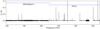 |
Fig. 1 APEX observations towards W Aql. The frequency ranges covered by the SEPIA/B5 and PI230 instruments are marked with blue horizontal lines. |
2 Observations
In the framework of a broader project in which the effect of AGB wind density on the circumstellar chemistry is studied, we carried out a spectral survey of W Aql in the range 159− 211 GHz using Band 5 of the Swedish-ESO PI Instrument (SEPIA; Billade et al. 2012; Belitsky et al. 2018) on the Atacama Pathfinder Experiment telescope (APEX; Güsten et al. 2006). The observations were carried out on 9 May 2017 in very good weather, at 0.8− 1.5 mm of precipitable water vapour (PWV). We obtained follow-up observations using the APEX/PI230 instrument1 on 17 and 21 May, 21 and 22 August, and 21 October 2018 with a PWV in the range 0.7− 1.0 mm, and on 2, 3, 7, and 11 July 2019 with a PWV in the range 0.9−5.8 mm.
All observations were carried out in wobbler-switching mode using the standard 50′′ beam throw. The size of the main beam is 30−39′′ at 159− 211 GHz (SEPIA/B5) and 27−30′′ at 209− 236 GHz and 23−25′′ at 244− 272 GHz (PI230).
We process the fully calibrated data with the GILDAS/CLASS2 package. After removing bad channels, which are typically present at < 50 MHz from the band edges, and masking relevant spectral features we remove a first-degree polynomial baseline from the spectra before averaging. We show the resulting spectra in  , the antenna temperature corrected for spillover and atmospheric losses, throughout the paper. A snapshot overview is shown in Fig. 1; for detailed spectra we refer to Figs. A.1 (SEPIA/B5) and A.2 (PI230). We refer to Appendix A for a brief discussion on the occurrence of a small number of features in the spectra that originate from sideband contamination.
Noise characteristics vary significantly throughout the covered spectral range and are summarised in Table 1. These values are approximate, as the rms noise can vary somewhat depending on the exact location in the spectrum as a consequence of different observing conditions (see above). The increase in rms noise in the SEPIA//B5 range is caused by the interference of atmospheric water around 183 GHz. The high noise in the range 252.0−255.8 GHz is a consequence of the short integration time at this frequency, connected to tuning problems. We include the data as they include several detected lines. The frequency resolution at which the rms noise values in Table 1 are measured translates to a velocity resolution in the range 5.5− 6.5 km s−1, allowing for detection of circumstellar spectral lines towards W Aql (see Sect. 3).
We adopt a systemic velocity vsys = −22.8 km s−1 for W Aql and all velocities v reported here are relative to this value within the local standard of rest (LSR) framework, that is v = vLSR − vsys.
Noise characteristics.
3 Results
We show the entire data set in Figs. A.1 (SEPIA/B5) and A.2 (PI230) and provide an overview of all measured emission features and their main characteristics in Table A.2. We summarise the identified molecules in Table 2.
We retain spectral features if the signal in at least three out of six consecutive channels of width Δν exceeds 3σ with σ and Δν equal to therms and frequency resolution listed in Table 1. This allows us to recover spectral lines over a total velocity interval of roughly two times the terminal velocity of W Aql, v∞ ≈ 16.5 km s−1 (Danilovich et al. 2014).
All lineidentifications stem from the Cologne Database for Molecular Spectroscopy3 (CDMS; Müller et al. 2001, 2005). We also used the catalogue for molecular line spectroscopy hosted by the Jet Propulsion Laboratory4 (JPL; Pickett et al. 1998)and Splatalogue5 as additional resources. Some features are reported as tentative detections although they may not strictly fulfill the above criterion. This is the case ifwe expect their presence based on other transitions or hyperfine components of the same transition of a given molecule and we find a plausible signal at a lower signal-to-noise ratio (S/N). Moreover, the combination of tentative detections of multiple transitions of a given molecule can lead to a firm detection of that molecule, as we discuss in Sect. 3.1.2 in the case of HC3N.
In Sect. 3.1 we summarise which molecules we identify in our observations, how our results compare to earlier reports on CSEs of M-, S-, and C-type AGB stars in general, and on the CSE of W Aql in particular. In Sect. 3.2 we shortly discuss the detection or non-detection of different isotopologues for some of the main elements.
Molecules identified in our survey towards W Aql.
3.1 Molecular inventory
We detect emission from transitions of CO, SiO, HCN, CS, SiS, and CN as expected for the CSE of an S-type AGB star and consistent with previous reports for W Aql (e.g. Brunner et al. 2018; Danilovich et al. 2014, 2018; Schöier et al. 2011). We additionally detect emission from species considered to be typical for, or until now only detected in, the CSEs of carbon-rich AGB stars: SiC2, SiN, C2 H, and the cyanopolyyne HC3N. We give an overview of these detections and provide some first abundance estimates to relate our findings to those made for M-type and C-type CSEs. We briefly address some tentative detections and unidentified emission features.
3.1.1 Previously detected: CO, SiO, HCN, CS, SiS, CN
CO, SiO, HCN, and CS are expected to form in relatively high abundances in the inner winds of all chemical types of AGB stars (Cherchneff 2006; Agúndez et al. 2020). SiS emission is also commonly detected towards CSEs around all chemical types of AGB stars (Schöier et al. 2013). We refer to the literature for detailed discussions on these molecules in the CSE of W Aql: Ramstedt & Olofsson (2014) and Danilovich et al. (2014) present radiative-transfer models of CO emission and Brunner et al. (2018) present models of SiO, HCN, CS, and SiS.
CO
We detect emission from 12CO(J = 2−1) and 13CO(J = 2−1) (see Fig. B.1), in agreement with the lines published by De Beck et al. (2010) and Ramstedt & Olofsson (2014) and with the calibration spectra made available by the APEX observatory6.
SiO
We detect three emission lines from the main SiO isotopologue (J = 4−3, 5−4, 6−5) and one from Si17O(J = 6−5) at 250.7 GHz. We do not detect emission from Si18O, in line with the intensity of the Si17O emission and the sensitivity reached in the spectra covering the relevant transitions of Si18O assuming 17O/18O = 1.2 (De Nutte et al. 2017). We detect the 29SiO(J = 4−3, 5−4) and 30SiO(J = 4−3, 5−4, 6−5) lines. An overview is shown in Fig. B.3.
HCN
We detect emission from HCN in the vibrational ground state v = 0 (J = 2−1, 3−2), from both l-type doubling components of J = 3−2 in the excited bending mode v2 = 1, and from H13CN (J = 2−1); see Fig. B.2.
CS
We detect emission from CS (J = 5−4) at 244.9 GHz with a peak intensity of 115 mK (≈4.5 Jy); see Fig. B.5. We do not detect emission from CS (J = 4−3) at 196.0 GHz and can set an upper limit to the peak intensity of 12 mK (≈ 0.5 Jy). The J = 5−4 intensity is roughly in line with the observed intensities of the J = 3−2, 6−5, 7−6 lines reported by Brunner et al. (2018), whereas the J = 4−3 upper limit lies far below the expectations. Cernicharo et al. (2014) report that low-J CS emissionlines show only small variability over time in the case of IRC +10 216, so we believe that time variability in the line excitation does not explain the observed discrepancy. Since we do not perform radiative transfer modelling for this paper, we wish to not hypothesise on the reason for the non-detection of the J = 4−3 line.
We detect emission from 13CS(J = 5−4) at 231.2 GHz at a peak intensity of ≈5 mK and can set an upper limit of 7 mK to the peak intensity of 13CS(J = 4−3) at 185.0 GHz. We also detect emission from C34S(J = 4−3) at 192.8 GHz.
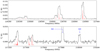 |
Fig. 2 CN emission; top: 12CN, bottom: 13CN. Vertical redlines indicate the position and relative strength of the hyperfine structure components of the rotational transition 2−1. |
SiS
We detect emission from the SiS transitions J = 9−8, 11− 10, 12−11, 13−12, 14−13 but do not detect SiS (J = 10−9) at 181.5 GHz owing to the higher noise in this region of the SEPIA/B5 spectrum; see Figs. A.1 and A.2 and Table 1. We also detect emission from the isotopologues 29SiS(J = 12−11, 14−13, 15−14), 30SiS(12−11, 13−12, 14−13,15−14), and Si34S (J = 12−11, 14−13, 15−14); see Fig. B.4.
CN
We detect emission over the full hyperfine structure of CN N = 2−1 between 226.2 and 227.0 GHz and of 13CN N = 2−1 between 217.2 and 217.5 GHz (Fig. 2). Whereas we report the first detection of 13CN towards W Aql, emission from CN (N = 1−0, 2−1) has been detected before with the IRAM-30m telescope (Bachiller et al. 1997), but at lower S/N than attained in the APEX data. Using Kelvin-to-Jansky conversion factors of 38 Jy K−1 for SEPIA/B5 (De Beck & Olofsson 2018, and references therein) and 7.2 Jy K−1 for the IRAM observations, in combination with a main-beam efficiency ηMB of 0.40 for the IRAM observations (Bachiller et al. 1997), we find that the peak fluxes for the strongest N = 2−1 features in Fig. 2 reach ≈3.8−4.6 Jy, whereas those measured by Bachiller et al. (1997) reach values of only ≈ 1.2−1.4 Jy. Without performing any further modelling, we hypothesise here that stellar variability might be responsible for this factor of approximately three difference in intensity, based on the conclusion by Bachiller et al. (1997) that radiative pumping through optical and near-infrared (NIR) bands likely dominates the CN excitation (calibration and/or pointing errors in the IRAM data cannot be excluded). The radiative-transfer models presented by Danilovich et al. (2014) for W Aql show an increase of CN at the photodissociation radius of HCN, in agreement with CN being produced as a photodissociation product of HCN. However, those models are only constrained by the N = 1−0 and N = 2−1 transitions and do not necessarily trace regions closer to the star or any possible variability of the emission over time.
3.1.2 New detections: SiC2, SiN, C2H, HC3N
SiC2
We detect fourteen emission lines pertaining to SiC2 (Fig. 3). We measure similar intensities for, for example, the 94,6 −84,5(213.2 GHz) and 94,5 −84,4 (213.3 GHz) lines and for the 114,8−104,7 (261.2 GHz) and 114,7−104,6 (261.5 GHz) lines. This is in line with the two transitions in each pair having almost identical intrinsic strengths and upper-level energies. The pairwise match in intensities confirms the identification of SiC2 in our spectra.
We construct a rotational temperature diagram for SiC2 based on the measured emission of 12 out of 14 detected transitions (Fig. 4). We leave out two transitions: 112,10−102,9 at 254.981 GHz because of the large uncertainty owing to very high rms noise in this spectral region and 120,12−110,11 at 261.990 GHz which is blended with a much stronger signal from C2H. We assume equal integrated intensity for the fully blended emission of the 106,5−96,4 and 106,4−96,3 transitions as they have identical transition probabilities (Einstein-A coefficients). Under the assumption of optically thin emission excited under LTE conditions, we find a rotational temperature Trot = 76 ± 28 K. We find a source-averaged column density of (2.1 ± 0.9) × 1014 cm−2 and an abundance SiC2/H2 ≈ 5 × 10⁻⁷ when assuming that the emission arises in a spherical shell located at 1− 2′′ in radius, that is, at a distance of ~ 400−800 AU from the star. The assumption of a peak in the SiC2 abundance at roughly 600 AU from the star is based on (1) the fact that one rotational temperature seems to represent all detected emission in our data reasonably well, (2) the location in the CSE where the derived rotational temperature is reached according to the temperature profile presented by Danilovich et al. (2014) is roughly 600 AU, and (3) the fact that SiC2 is also observed in a shell around IRC +10 216 (Velilla-Prieto et al. 2019). However, the SiC2 emission towards IRC +10 216 is located in a shell at ~14−16′′ from the central star, which is at roughly three times larger physical separation from the central star compared to what we assume for W Aql. Assuming the equivalent spatial distribution for SiC2 in W Aql’s CSE, we obtain a slightly higher abundance SiC2/H2 ≈ 8 × 10⁻⁷, which is still well within the uncertainties of our simple approach here7. The difference in spatial occurrence of SiC2 could be a consequence of the roughly three times higher mass-loss rate of IRC +10 216, and hence the correspondingly higher densities in the CSE. Comparing our estimated abundance to the results presented by Massalkhi et al. (2018, see their Fig. 6) for a sample of 25 C-rich envelopes, we find that the combination of the SiC2 abundance and wind density Ṁ∕v∞ of W Aql fits well within the distribution of the C-rich envelopes, with W Aql’s SiC2 abundance being on the lower end of the presented sample. Accounting for the uncertainties inherent to our approach, we conclude that this result indicates a possible similarity in chemistry between the CSE of the S-type AGB star W Aql and C-type AGB stars.
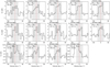 |
Fig. 3 SiC2 emission. Shaded areas indicate the part of the spectrum integrated to obtain the intensities used to construct the rotational diagram in Fig. 4, and vertical red lines correspond to the rest frequency, centred to a velocity of 0 km s−1. We give the rest frequency, quantum numbers, and upper level energy for each transition. We note that (i) the rest frequencies of the 106,5−96,4 and 106,4−96,3 lines at 235.7 GHz differ by only 0.1 MHz and (ii) the emission from the 120,12 − 110,11 transition at 261.991 GHz (last panel) is blended with intense C2H emission (Fig. 5) and is therefore omitted from the rotational diagram analysis, as is the 112,10 − 102,9 transition which is tentatively detected in a region of high rms noise. |
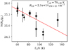 |
Fig. 4 Rotational temperature diagram for SiC2. |
SiN
We detect emission from the strongest components of the SiN (N = 5−4) transition at 218.01 and 218.51 GHz and of N = 6−5 at 261.65 and 262.15 GHz (Figs. 5 and B.6; these components have ΔF = ΔJ). Assuming similar line strengths, the non-detection of the N = 4−3 lines at 174.36 and 174.86 GHz is in line with the much higher rms-noise in that region. The hyperfine structure of the SiN transition isnot resolved and has a very limited contribution of only about 1 MHz to the broadening of the overall profile.
We can directly compare our APEX observations of SiN (N = 6−5) towards W Aql to the NRAO 12 m telescope observations of SiN (N = 6−5) towards IRC+10 216 (Turner 1992). Scaling the emission for mass-loss rate and distance (W Aql: Ṁ = 3 × 10⁻⁶ M⊙ yr−1, d = 395 pc; IRC +10 216: Ṁ = 2 × 10⁻⁵ M⊙ yr−1, d = 130 pc; Brunner et al. 2018; Agúndez et al. 2012; Men’shchikov et al. 2001) we find that the SiN emission in W Aql is roughly five times as bright as the SiN emission in IRC +10 216 (for N = 6−5). Assuming optically thin emission and the same excitation conditions for SiN in both CSEs, this would imply (SiN/H2)W Aql ≈ 5 × (SiN/H2)IRC +10 216 = 4 × 10⁻⁸ (Agúndez 2009).
SiN and SiC2 have both been detected towards the CSEs of C-type stars, but we are not aware of any reported detections of either molecule towards S-type or M-type AGB stars. Based on the angular resolution of 24–29′′ obtained in the APEX observations of SiC2 and SiN we cannot determine whether these molecules are present in the extended CSE of W Aql or only close to the star, but from the width of the line profiles we find that both the SiC2 and SiN emitting gas reach the terminal velocity of the wind, v∞ ≈ 16.5 km s−1 (Danilovich et al. 2014), suggesting that both molecules are present beyond the wind-acceleration zone. Furthermore, in the case of SiC2, we determine a single rotational temperature low enough to be indicative of the presence of the molecule in the outer parts of the CSE (Danilovich et al. 2014, see their Figs. 3 and 4).
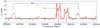 |
Fig. 5 C2H and SiN emission. High-signal-to-noise ratio detection of C2H (3−2) in the PI230 data, plotted at 3.0 MHz (≈3.5 km s−1) spectral resolution. Vertical red lines indicate the position and relative strength of the hyperfine structure components of the rotational transition of C2H. In red, we overplot a synthetic spectrum of C2H (3−2) using a “shell” profile as described in the GILDAS/CLASS manual, fitted to the data by eye, using the intrinsic component strengths. In blue we indicate the location of the strongest components of the SiN (N = 6−5) transition; see Fig. B.6 for all detected SiN emission. We mark the rest frequency of SiC2 (120,12−110,11) in green. |
C2H
We tentatively detect emission from C2H in the N = 2−1 transition at ~174.7 GHz, and detect emission at high signal-to-noise ratio for N = 3−2 at ~262.0 GHz (Fig. 5). We produce a synthetic spectrum for the N = 3−2 transition assuming a “shell” profile for each hyperfine component, as described in the GILDAS/CLASS manual, and using the tabulated intrinsic relative strengths and fit the sum of them to our data by eye (see Fig. 5). We find that the measured relative strengths of the hyperfine structure components agree very well with the intrinsic relative strengths tabulated in the CDMS (Müller et al. 2000).
The line profiles of the doublet components of C2 H (N = 3−2) are double-peaked, but we note that the peaks corresponding to the extreme velocities of the doublet components are not equal in strength, the blueshifted peaks being much stronger than the redshifted peaks in both components. The strong difference between the blue and red sides of the profiles hints at an asymmetry in the CSE with more C2 H gas excited in the part of the CSE moving towards the observer. We cannot assess whether this would be caused by differences in excitation or in abundance distribution. Both of these could be a consequence of, for example, clumpiness in the CSE.
We also note that roughly the opposite is true in the C2 H spectra towards IRC +10 216, where the redshifted peaks are stronger than the blueshifted peaks in the transitions 1− 0, …, 7−6 presented by De Beck et al. (2012). In the case of IRC +10 216, the difference is likely a consequence of optical-depth effects, where only the outermost and therefore colder C2H gas is visible in the front of the CSE, whereas we only see the emission from the warmer, inner C2 H gas from the part of the CSE that moves away from the observer. In the case of IRC +10 216, we know that the C2 H emission is spread over a thin, circular shell around the star. In the case of W Aql we lack direct information on the spatial distribution of the excited C2H gas, but the double-peaked spectrum suggests emission from a shell.
Scaling the measured C2H line emission for IRC +10 216 to what one could expect at the distance of W Aql and assuming for simplicity that the emission is excited in a similar shell-like region around the star and that the line intensity scales linearly with Ṁ, we expect the strongest components to peak at ~10−15 mK for N = 2−1 and N = 3−2 in our APEX data. Since the observed lines peak at ~5−15 mK, we suggest that the abundance of C2H in the CSE of W Aql is roughly a factor of two lower than in the CSE of IRC +10 216, that is (C2 H/H2)W Aql ≈ 0.5 × (C2H/H2)IRC +10 216 = 1 × 10⁻⁵ (De Beck et al. 2012). Cernicharo et al. (2014) note that the strength of the C2 H emission in IRC +10 216 is highly variable with time as a consequence of the strong effect of radiative pumping in the molecular excitation and the changes in the stellar radiation field owing to pulsations. However, since we consider here a low-N rotational transition, this variability is likely limited to within the observational uncertainties (see their Fig. 2). We do not detect any emission from the longer-chain radicals C4H or C6H at the current sensitivity.
HC3N
We tentatively detect emission in multiple rotational transitions from HC3N. Figure 6 shows an overview of the spectral ranges where rotational transitions of HC3N are covered by our data. Some transitions are not detected (marked ND) and some are tentatively detected (marked T). We also show the result of stacking the data, aligned in velocity space, weighted with the ratio of the statistical weights 2J + 1 of the upper levels of the respective transitions J → J − 1 and the rms noise in the spectrum close to the transition’s rest frequency. We performed this stacking procedure for three sets of lines; we obtain S∕N > 5 when stacking the tentative detections, do not find significant structure when stacking the non-detections, and find that the tentative detections weigh strong enough to give rise to line-like structure also in the total stacked profile. This is a direct result of the higher rms noise in the parts of the spectrum with the non-detections, making these less significant.
Based on the multiple tentative detections and the results from the stacking procedure we are confident that we detect HC3N in the CSE of W Aql. To the best of our knowledge, it is the first time such a carbon-chain molecule has been seen in the CSE of an S-type star and it has not yet been detected in the CSE of an M-type AGB star. Comparing the line peak intensities to those reported by Tenenbaum et al. (2010) for IRC +10 216, we find that the emission is weaker in W Aql by a factor 10− 15, accounting for the difference in distance and mass-loss rate. This implies that HC3N is roughly one to two orders of magnitude less abundant in the CSE of W Aql than around IRC +10 216 and leads to a first estimate of a fractional abundance on the order10−7−10−8 (Agúndez 2009).
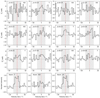 |
Fig. 6 Detection of HC3N emission. Top three rows: spectra extracted around all frequencies of HC3N rotational transitions in the vibrational ground state v = 0 covered by our observations. Shaded areas indicate a velocity range [−25, 25] km s−1 around the rest frequency of the transition, and vertical red lines correspond to the rest frequency centred to a velocity of 0 km s−1. All panels are labelled with the transition and whether the line is considered tentatively detected (T) or not detected (ND). Bottom row: result of stacking the emission for selected transitions, aligned in velocity space: left: tentatively identified transitions (marked T), middle: transitions not detected (marked ND), right: all twelve transitions shown in the top three rows. We note that the intensity scale is normalised to the peak and has no physical meaning as such. |
3.1.3 Tentative detections
HNC
We tentatively detect emission from HN13C (J = 3−2) at 261.3 GHz at a peak-signal-to-noise ratio (peak-S/N) of ≈3; see Fig. 7a. For this tentative detection, and those of NaCl and HCO+ discussed below, we quote S/N values of line profile fits based on the “shell” profile as defined in the GILDAS/CLASS manual, using the rms noise in the line-free part of the spectra at [−200;−50] km s−1.
We do not detect emission from HN13C (J = 2−1) at 174.2 GHz or HNC (J = 2−1) at 181.3 GHz, in line with the sensitivity reached in our data set at the relevant frequencies. Assuming optically thin emission from both H13CN and HN13C we obtain an abundance ratio HN13C/H13CN of the order 0.01−0.1. Values reported in the literature for the abundance ratio HNC/HCN are anywhere in the range 0.001 and 0.1 for the CSEs of the C-type AGB star IRC +10 216 and the supergiant VY CMa (Johansson et al. 1984; Daniel et al. 2012; Ziurys et al. 2009). For the remainder of the paper, we assume that HNC/H2 = 0.01 ×HCN/H2 = 3.1 × 10⁻⁸ (Danilovich et al. 2014) with one order of magnitude uncertainty in both directions, in agreement with our HN13C measurements and the above literature values.
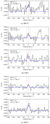 |
Fig. 7 Tentative detections. Red vertical lines correspond to the rest frequencies of the transitions; grey vertical lines indicate the 16.5 km s−1 expansion velocity of the CSE of W Aql; blue fits were produced using the “shell” profile function as defined in the GILDAS/CLASS package. The velocity resolution at which the spectra are presented is listed in each panel. |
NaCl
We tentatively detect NaCl (J = 19−18, 20−19) at 247.2 and 260.2 GHz; see Fig. 7b. We obtain peak-S/N of ≈ 2 and integrated-signal-to-noise ratios of ≈4 for both transitions. The non-detections of NaCl emission in the SEPIA-B5 data are consistent with the higher rms noise in those observations. Based on a comparison to the IK Tau spectrum presented by Velilla Prieto et al. (2017) we estimate that  ; and based on the NaCl detections towards IRC +10 216 (Agúndez et al. 2012) we estimate that
  . This leads to an estimate for
  on the order of a few 10−8. The current data do not provide reliable information on which part of the CSE this emission originates from and follow-up observationsat higher sensitivity are needed to draw any firm conclusions on the presence, abundance, and/or location of NaCl in the CSE. NaCl emission has been detected around both M-type and C-type AGB stars (e.g. Agúndez et al. 2012; De Beck et al. 2015; De Beck & Olofsson 2018), but we are not aware of any reported detection towards S-type stars.
HCO+
We tentatively detect emission from HCO+ (J = 3−2) at 267.6 GHz at a peak-signal-to-noise ratio of ≈4; see Fig. 7c. There clearly is emission at this position in the spectrum, but we cannot firmly claim that HCO+ is the carrier since we have no other detected transition towards W Aql to confirm this. However, based on the tentative identification, we also present the spectrum at 178.4 GHz, where the HCO+ (J = 2−1) transition lies. We cannot claim a detection, but do observe structure in the spectrum suggestive of a low-intensity emission line at the correct position. Confirmation will require sensitive follow-up observations of multiple transitions.
HCO+ has been detected in the CSEs of the M-type AGB stars IK Tau, TX Cam, and W Hya (Pulliam et al. 2011), in the bipolar lobes around the peculiar OH/IR star OH 231.8+4.2 (Sánchez Contreras et al. 2015), and around the supergiants VY CMa and NML Cyg (Ziurys et al. 2007, 2009; Pulliam et al. 2011). All of these CSEs display an oxygen-rich chemistry. Typical abundances HCO+/H2 range around 10−8−10−7. HCO+ has also been detected in the CSE of IRC +10 216 (Agúndez & Cernicharo 2006; Pulliam et al. 2011, and references therein), but its abundance in that case is as low as a few 10−9. IRC +10 216 is currently the only C-type AGB star for which such a detection has been reported. The emission (suspected) from HCO+ (3−2) towards W Aql is a factor of roughly 3, 7, and 40 stronger than those reported by Pulliam et al. (2011) towards TX Cam, IK Tau, and IRC +10 216, respectively, accounting for the mass-loss rates, distances, and difference in beam size between APEX and the SMT. We assume for the remainder of the paper that  (Velilla Prieto et al. 2017).
3.1.4 Upper limits
SO, SO2
We do not detect emission from SO or SO2 in our spectra of W Aql, whereas these are dominant in the spectra of the M-type AGB stars R Dor and IK Tau (De Beck & Olofsson 2018; Velilla Prieto et al. 2017). From a comparison with scaled spectra of R Dor and IK Tau in the SEPIA/B5 range (De Beck & Olofsson 2018; Velilla Prieto et al. 2017, and De Beck et al., in prep.), accounting for the differences in distance and mass-loss rate (dR Dor = 59 pc, ṀR Dor = 2 × 10⁻⁷ M⊙ yr−1, dIK Tau = 250 pc, ṀIK Tau = 8 × 10⁻⁶ M⊙ yr−1; Maercker et al. 2016; Decin et al. 2010), we set the SO2 abundance of R Dor (5 × 10⁻⁶) and the SO abundance of IK Tau (1 × 10⁻⁶) as upper limits for the respective abundances in the CSE of W Aql. We discuss these differences and possible implications for the sulphur chemistry in Sect. 4.
H2S
We do not detect emission from H2S in our spectra, although we obtained data at slightly higher sensitivity than Danilovich et al. (2017). From a direct comparison to the line emission from IK Tau reported by Danilovich et al. (2017), we set an upper limit  (Danilovich et al. 2017).
PN, PO
Similarly, we derive an upper limit  based on the comparison of our observations to the emission spectrum of PN (J = 5−4) presented by Velilla Prieto et al. (2017). A comparison to the spectra presented by Milam et al. (2008) for IRC +10 216 does not set additional constraints as the scaled intensity lies far below the sensitivity reached in our observations. Unfortunately, we cannot derive an upper limit for the PO abundance towards W Aql as the sensitivity of the IK Tau spectrum obtained with SEPIA/B5 (scaled for d and Ṁ) is superior by a factor of approximately eight to that of the W Aql spectrum and the PO transition at 196 GHz remains undetected in both spectra.
3.1.5 Unidentified lines
We find only two unidentified features in this rather broad spectral coverage. Figure B.7 shows emission features in our spectra that we cannot identify with any known carriers. We can rule out contamination of the spectrum through the image sideband for all of these. Two of the three features lie immediately adjacent to each other, are similar in intensity, and are located close to the 29SiS(v = 3, J = 14−13) line. With the current sensitivity of the data we cannot rule out that these two features (at 249393 ± 4 and ≈ 249410 MHz) are actually part of the same emission line, centred at 249402 ± 4 MHz.
Another unidentified feature is centred at 267073 ± 4 MHz and seems double-peaked. We cannot identify any possible carrier within 15 MHz of the presumed central frequency.
3.2 Isotopes
Isotopic ratios can ideally be used to help constrain the initial mass of the star and its current evolutionary status. We present estimates of isotopic abundance ratios in Table 3. These are assumed to be represented by the abundance ratios Ra ∕b of isotopologues a and b, estimated according to
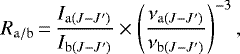 (1)
(1)
using the integrated line strengths I of transitions J−J′ for isotopologues a and b and taking into account the difference in intrinsic line strengths between the isotopologue transitions and telescope beamwidths at the rest frequencies. This simple method assumes that the same transition J− J′ for two isotopologues is excited under similar conditions.
Isotopologue ratios retrieved from frequency-corrected line-intensity ratios Rc, as described in the text.
Carbon
From radiative transfer modelling of multiple emission lines from both 12CO and 13CO, Ramstedt & Olofsson (2014) and Danilovich et al. (2014) derived 12C/13C of 26 and 29, respectively. We do not attempt such modelling here, but it is clear that the CO, HCN, CS, and CN emission are affected by optical-depth effects since the relevant line intensity ratios are much lower than this (see Table 3).
Oxygen
The detections of C17O(J = 2−1) and C18O (J = 2−1) lead to an estimate of C17O∕C18O = 1.0 ± 0.4. We note that the C18O emission in our data appears blended with an unidentified source of emission, increasing the uncertainty on this estimate. This component is not visible in the spectra presented by De Nutte et al. (2017) owing to their higher noise. We detect emission from Si17O(J = 6−5), but not from Si18O(J = 6−5). This non-detection is in line with the achieved sensitivity, when considering the above results.
Silicon
We detect emission from multiple transitions of 28SiO, 29SiO, 30SiO and 28SiS, 29SiS, 30SiS; see Figs. B.3 and B.4. However, based on the ratios sampled by the different transitions, it is clear that optical-depth effects need to be accounted for in order to derive reliable isotopic ratios. For example, we find 28Si ∕29Si isotopologue line intensity ratios spanning the range 7−20 and 28Si∕30Si spanning the range 8−28. However, detailed abundance modelling using non-local thermodynamical equilibrium (non-LTE) radiative-transfer models is beyond the scope of this paper.
Sulphur
We detect Si32S and Si34S, and C32S and C34S. We do not detect any carriers of 33S, the least abundant sulphur isotope. The uneven sampling of the spectrum of the different isotopologues prevents estimates of the isotopic ratios without detailed modelling.
Initial stellar mass
Danilovich et al. (2015) constrained the current mass of W Aql to be in the range 1.04−3M⊙. De Nutte et al. (2017) derived an initial mass Mi = 1.59 ± 0.08M⊙ based on their analysis of C17O and C18O emission. Using our observations we derive an initial-mass estimate of Mi = 1.6 ± 0.2M⊙. Both our estimate and the one of De Nutte et al. (2017) are based only on the relative emission strengths of the J = 2−1 transitions of C17O and C18O. The derived initial mass appears consistent with the fact that evolutionary models predict only stars with initial mass above ~1.5 M⊙ (e.g. Hinkle et al. 2016) to undergo third dredge-up events, a necessary process to bring s-process elements to the surface and move the star from M-type to S-type. Hinkle et al. (2016) report that their model for a star with Mi = 1.6M⊙ reaches a C∕O = 1 when 12C/13C reaches 28. The reported C/O and 12C/13C and our derived initial mass therefore all fit into one consistent picture of W Aql as a star close to its transition from being oxygen-rich to becoming carbon-rich.
4 Discussion
Based on the classification scheme of Keenan & Boeshaar (1980), Danilovich et al. (2015) reported a spectral type S6/6e and a C/O = 0.98, making W Aql an S-type star that is close to having a carbon-rich atmosphere. On the other hand, based on the presence of emission from SiN, SiC2, C2 H, and HC3N in the CSE, one may classify the content of W Aql’s CSE as (rather) carbon-rich. This apparent contrast requires further discussion. In this section we compare the appearance of the atmosphere of W Aql and the surrounding circumstellar gas and dust to what we know about other AGB stars.
4.1 Atmosphere
Hony et al. (2009) reported the presence of HCN, C2H2, and C3 absorption bands towards W Aql in the mid-infrared ISO data, but did not discuss this. These molecules are typical for C-type atmospheres, but their formation is maybe possible also in atmospheres of stars with C/O ≲ 1 as a consequence of the non-equilibrium chemistry induced by shocks that travel through the atmosphere and can free atomic carbon due to the destruction of, mainly, CO. Although the models presented by Cherchneff (2006) indeed show an increase in C2H2 abundance in the presence of shocks compared to thermal equilibrium, they also show an approximately three orders of magnitude drop in the C2H2 abundance at 5 R⋆ when varying C/O from 1 down to 0.98 (see their Fig. 7). The predicted fractional abundance in the latter case, ≈10−9, is still more than five orders of magnitude higher than for stars with C/O < 0.9. For reference, IRC +10 216 has a derived C2H2 abundance of 8 × 10⁻⁵ in the inner CSE (within 40 stellar radii; Fonfría et al. 2008, and references therein). The models presented by Agúndez et al. (2020) indicate that, even under the assumption of chemical equilibrium, the molecular gas around S-type stars with C/O ≈ 1 could resemble that around C-type stars quite closely, with similar abundances of for example C2H2 and HCN in the atmosphere for C/O in the range 0.98−1.02. The presence of C2 H2 in the stellar atmosphere of W Aql explains the presence of C2 H in its circumstellar environment, as the radical is the direct photodissociation product. The presence of both C2 H2 and HCN in the atmosphere can explain the presence of HC3N in the CSE according to the chemical models of Cordiner & Millar (2009).
W Aql is a Mira star with a variability in the visual ΔV ≈ 7 mag. Such stars populate region C in the (K − [12], [25] − [60]) colour–colour diagrams presented by Jorissen & Knapp (1998). Van Eck et al. (2017) point out that strong variability can significantly affect the estimated atmospheric parameters such as the effective temperature, surface gravity, C/O, and s-process enrichment [s/Fe]. Keenan & Boeshaar (1980) report observations of W Aql at only three different phases, making it difficult to assess this potential variability. It is beyond the scope of this paper to quantify the possible effect of photometric variability on the estimated C/O. However, we repeat that the absence of TiO lines and the presence of strong Na D lines put W Aql close to the C-type classification, whereas the presence of ZrO bands points at W Aql not yet being sufficiently enriched to be C-type.
4.2 Circumstellar gas
Figure 8 is central to our discussion on how the circumstellar chemistry of W Aql compares to that of other AGB CSEs. We show estimated peak fractional abundances for CSEs around a small collection of AGB stars: the two M-type stars R Dor and IK Tau, the two S-type stars χ Cyg and W Aql, and the two C-type stars V Aql and IRC +10 216. For all three chemical types the former star has a mass-loss rate in the range 0.1−0.7 × 10⁻⁶ M⊙ yr−1 and the latter in the range 3.0−20 × 10−6 M⊙ yr−1. For a few molecules, we also show median values for different chemical types based on sample studies8 and list the used peak fractional abundances and the references to the relevant studies in Table C.1.
Danilovich et al. (2014) found that their derived circumstellar abundances of HCN, SiO, and H2O for W Aql are between those typical for M- and C-type AGB stars, from which they conclude that the abundances are consistent with an S-type classification. Schöier et al. (2013) reported that the HCN abundance in S-type CSEs is indeed intermediate between those in CSEs of M-type and C-type AGB stars.
Contrary to the fact that the CSE of W Aql seems to have chemical properties intermediate between the M-type and C-type classes when looking at the most common candidates such as CS, SiS, HCN, and SiO, we estimate high abundances of C2H, CN, SiC2, and SiN, and likely also of HC3N, and HNC. All of these molecules are expected around C-type stars and are not seen around M-type stars. Given that C/O < 1 for S-type stars like W Aql, one does not, at first sight, expect such a carbon-rich chemistry as we report in Sect. 3 and show in Fig. 8. For molecules where CSEs from M-type stars exhibit markedly higher abundances than those from C-type stars, for example H2S, PN, PO, SO, and SO2, we have no estimates or only upper limits for the case of W Aql. From our results and the abundances reported in the literature and compiled in Fig. 8 it seems that W Aql’s CSE is closer to that of IRC +10 216 in its gas-phase chemistry than to that of IK Tau, whereas all three stars have roughly similar wind properties (expansion velocity and mass-loss rate). Only in the cases of H2O and NH3 are the abundances for W Aql closer to those for IK Tau than to those for IRC +10 216; for SiO, the reported abundance is exactly intermediate9. In the case of NH3, W Aql’s abundance exceeds that of IK Tau, removing it entirely from an intermediate status. We note, though, that the excitation of all three molecules (H2O, NH3, and SiO) is predominantly through the strongly variable radiation field, possibly introducing considerable uncertainties on the derived abundances (for all objects).
Currently, it is difficult to assess the differences or similarities between the CSE of W Aql (C/O = 0.98) on the one hand, and that of χ Cyg (C/O ≤ 0.95; based on the measurements and classification scheme presented by Keenan & Boeshaar 1980) on the other, as broad, sensitive observations of χ Cyg are currently missing. The chemical equilibrium models of Agúndez et al. (2020) provide support for an inner-wind chemistry around W Aql closely resembling that of a C-type AGB star. However, the molecules we detect that are “typical for C-rich CSEs” are found in the outer CSE and there are currently no chemical models available that describe the chemical content of the CSEs of S-type AGB stars on that physical scale. Because of this and the lack of observational characterisation of the CSEs of S-type stars with different C/O, we cannot yet assess in a straightforward way how (un)typical the CSE of W Aql is. Chemical models must explore the impact of the atmospheric C/O on the circumstellar abundances.
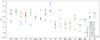 |
Fig. 8 Peak molecular abundances in the CSEs of AGB stars of different chemical types: M-type stars R Dor and IK Tau, S-type stars χ Cyg and W Aql, and C-type stars V Aql and IRC +10 216. We note that the high SiS abundance for IK Tau is only representative of a geometrically small component centred on the star, after which depletion is very efficient and the abundance drops roughly four orders of magnitude. See text for further discussion and references. We have included error bars only for W Aql for the sake of visibility. The error bars correspond to the values specified in Table C.1 and we note that they are often smaller than the plotting symbol. Upper limits are indicated with downwards arrows. Molecules that were not previously identified towards W Aql are highlighted in boldface font on the horizontal axis. |
4.3 Dust
Hony et al. (2009) proposed the presence of non-stoichiometric silicates around S-type stars to explain the substantial spectral differences in the infrared between CSEs of S-type and M-type AGB stars, which is plausible since stars with C∕O ~ 1 exhibit an increased Mg/SiO4 abundance ratio, with less free oxygen available when dust forms. Additionally, the latter authors reported the presence of the 30 μm feature, attributed to MgS, in the ISO spectrum of W Aql and π1 Gru, another S-type star. This feature is typical for carbon-rich CSEs and is seen only for S-type AGB stars with a C/O > 0.96 (Smolders et al. 2012, their group III stars). MgS is suggested to be present in mantles covering dust grains such as for example amorphous alumina. No estimate is available for the amount of S that would be bound in MgS dust. Hony et al. (2009) also mentioned the possibility of SiC dust in the spectrum of W Aql, at ~11 and ~17 μm, another dust species typical of C-rich CSEs. It is unclear whether the W Aql spectrum shows a contributionfrom amorphous carbon dust, which typically accounts for several tens of percent of the dust mass in carbon-rich CSEs. Furthermore, the W Aql spectrum lacks the amorphous silicate feature at 18 μm and lacks a clear silicate feature at 20 μm. We are not aware of radiative transfer models of W Aql exploring the dust composition in detail.
4.4 Influence from the binary companion?
Danilovich et al. (2015) found that the binary companion is a main-sequence dwarf star of spectral type F8 – G0. It is unlikely that this dwarf star has a significant influence on the photochemistry in the CSE of the AGB star. Based on ALMA observations, Ramstedt et al. (2017) show that the binary companion has a rather weak but measurable effect on the CSE morphology. Locally increased densities could cause changes in the circumstellar chemistry. However, the emission lines reported here are detected with APEX, a single-dish telescope, and are most likely more representative of the overall CSE chemistry rather than of localised deviations.
5 Conclusions
We observed the CSE of the S-type AGB star W Aql with APEX at 159−211 GHz using the SEPIA/B5 instrument, and in the frequency windows 208.4−239.8, 244.2−255.8, and 260.0−267.8 GHz using the PI230 instrument. We report a number of new detections towards this CSE, including C2 H, SiN, SiC2, and HC3N, all of which are molecules previously reported only towards C-rich CSEs. We tentatively detect HN13C, NaCl, and HCO+. We made some first estimates of the molecular abundances, and compared these to abundances reported for CSEs of M-type and C-type AGB stars. We find that the CSE of W Aql is more similar to that of a C-type AGB star than to that of an M-type AGB star with similar wind properties, in agreement with the recent chemical equilibrium models of Agúndez et al. (2020). We cannot currently assess how typical the abundances in W Aql’s CSE are for S-type CSEs: observations have not yet extensively covered the parameter space of S-type star CSEs, in terms of wind density, C/O, and chemical content, and chemical models of the outer CSE of S-type stars are lacking.
As the ISO observations of W Aql show signatures of C2 H2 and HCN in the atmosphere and of MgS and SiC in the dust, our detections of molecular gas deemed typical for carbon-rich stars should perhaps not be entirely unexpected. However, previous abundance derivations for commonly targeted molecules such as SiO, SiS, HCN, and CS have consistently led to the conclusion that W Aql appears to be a rather typical S-type star, with abundances intermediate to those characteristic for CSEs around C-type and M-type stars. It is only now, with the presented frequency coverage, that the possibly more carbonaceous nature of W Aql’s molecular CSE becomes apparent.
We hope that our findings on W Aql can spark increased interest in the chemical diversity in the stellar CSEs that comes along with the chemical evolution of the AGB stars themselves. Broader inventories, both in terms of targets and frequency ranges, of the molecular content of CSEs around M-type and S-type stars in particular are essential to constrain comprehensive chemical models. Strong constraints on the gas content are also essential to understand the dust formation and dust growth taking place close to the star.
Acknowledgements
E.D.B. acknowledges financial support from the Swedish National Space Agency. H.O. acknowledges financial support from the Swedish Research Council. Based on observations with the Atacama Pathfinder EXperiment (APEX) telescope. APEX is a collaboration between the Max Planck Institute for Radio Astronomy, the European Southern Observatory, and the Onsala Space Observatory. Swedish observations on APEX are supported through Swedish Research Council grant No 2017-00648. The APEX observations were obtained under project numbers O-099.F-9306 (SEPIA/B5) and O-0101.F-9312, O-0102.F-9313, and O-0103.F-9319 (PI230).
Appendix A Data presentation
A.1 Data contamination
We detect five features in our spectra that are leakage from strong lines in the image sideband of a given frequency setup; see Table A.1. In the SEPIA/B5-data the leakage corresponds to a suppression of the signal at 26 dB, which is significantly better than the average 18.5 dB suppression reported for SEPIA/B5 (Humphreys et al. 2017; Belitsky et al. 2018). In the PI230 data we find image leakage at suppression levels between 24 and 36 dB.
A.2 Spectra
We show the complete spectra obtained with SEPIA/B5 in Fig. A.1 and for PI230 in Fig. A.2. Both are displayed at a resolution of7.5 km s−1.
Image sideband leakage from strong lines.
A.3 Line properties
All features that have been detected in our observations and marked in Figs. A.1 and A.2 are listed in Table A.2. We report the extent of the line in velocity range [vmin, vmax] and the integrated intensity across this range with a 2σ error. Comments in the table relate to, for example, tentative detections, blends, or hyperfine structure. We note that the velocity ranges are not necessarily symmetric around 0 km s−1 since they were derived to account for weak wings of emission seen for some of the lines. A detailed study of the physical structures within the CSE traced by different molecular transitions is beyond the scope of this paper and would benefit from spatially resolved observations.
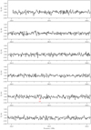 |
Fig. A.1 APEX SEPIA/B5 line survey of W Aql. Labels show the carrier molecule of the indicated emission. Red labels indicate tentative or unidentified detections. Purple labels (Im(...)) pertain to emission contaminating the signal from the image sideband (see Sect. 2). For visibility, some parts of the survey were rescaled to fit the vertical scale. The colour coding of the spectrum corresponds to the following scale factors: (black) 1; (green) 1/5. We note that the labellingat frequencies above 209.0 GHz is based on identifications in the PI230 spectrum and is shown here only for reference. |
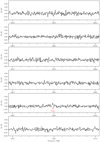 |
Fig. A.1 continued. |
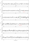 |
Fig. A.1 continued. |
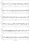 |
Fig. A.1 continued. |
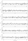 |
Fig. A.1 continued. |
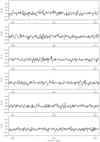 |
Fig. A.1 continued. |
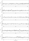 |
Fig. A.1 continued. |
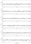 |
Fig. A.1 continued. |
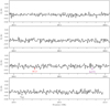 |
Fig. A.1 continued. |
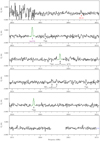 |
Fig. A.2 APEX line survey of W Aql. Labels show the carrier molecule of the indicated emission. Red labels indicate tentative or unidentified detections. Purple labels (Im(...)) pertain to emission contaminating the signal from the image sideband (see Sect. 2). For visibility, some parts of the survey were rescaled to fit the vertical scale. The colour coding of the spectrum corresponds to the following scale factors: (black) 1; (green) 1/5; (blue) 1/25; (magenta) 1/125; (orange) 1/250. |
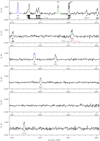 |
Fig. A.2 continued. |
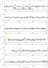 |
Fig. A.2 continued. |
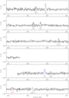 |
Fig. A.2 continued. |
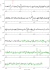 |
Fig. A.2 continued. |
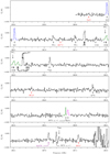 |
Fig. A.2 continued. |
Molecular lines detected in our survey towards W Aql.
Appendix B Detections
This appendix features all line emission detected in the spectra in Appendix A other than the lines presented in the body of the paper. In all of these figures the grey-shaded area designates the spectral range specified in Table A.2 and used to calculate the listed integrated intensities.
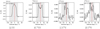 |
Fig. B.1 CO emission. |
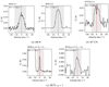 |
Fig. B.2 HCN emission. |
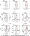 |
Fig. B.3 SiOemission. |
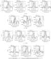 |
Fig. B.4 SiS emission. |
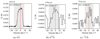 |
Fig. B.5 CS emission. |
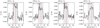 |
Fig. B.6 SiN emission. Rest frequencies were calculated by weighting the hyperfine component frequencies with the intrinsic component intensities. |
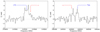 |
Fig. B.7 Unidentified emission features. |
Appendix C Fractional abundances for M-, S-, C-type CSEs
The peak fractional abundances used to compile Fig. 8 are listed in Table C.1, along with the references to the relevant studies and a marker in case of upper limits. We refer to those papers for presentation of and discussion on the modelling procedures used to estimate the abundances and the target samples used to obtain median abundance values for M-type, S-type, and C-type stars.
References
- Agúndez, M. 2009, PhD thesis, Departamento de Astrofisica, Madrid, Spain [Google Scholar]
- Agúndez, M.,& Cernicharo, J. 2006, ApJ, 650, 374 [NASA ADS] [CrossRef] [Google Scholar]
- Agúndez, M., Fonfría, J. P., Cernicharo, J., et al. 2012, A&A, 543, A48 [NASA ADS] [CrossRef] [EDP Sciences] [Google Scholar]
- Agúndez, M., Martinez, J. I., de Andres, P. L., Cernicharo, J., & Martin-Gago, J. A. 2020, A&A 637, A59 [CrossRef] [EDP Sciences] [Google Scholar]
- Alfonso-Garzón, J., Domingo, A., Mas-Hesse, J. M., & Giménez, A. 2012, A&A, 548, A79 [NASA ADS] [CrossRef] [EDP Sciences] [Google Scholar]
- Asplund, M., Grevesse, N., Sauval, A. J., & Scott, P. 2009, ARA&A, 47, 481 [NASA ADS] [CrossRef] [Google Scholar]
- Bachiller, R., Fuente, A., Bujarrabal, V., et al. 1997, A&A, 319, 235 [NASA ADS] [Google Scholar]
- Belitsky, V., Lapkin, I., Fredrixon, M., et al. 2018, A&A, 612, A23 [NASA ADS] [CrossRef] [EDP Sciences] [Google Scholar]
- Billade, B., Nyström, O., Meledin, D., et al. 2012, IEEE Trans. Terahertz Sci. Technol., 2, 208 [NASA ADS] [CrossRef] [Google Scholar]
- Brunner, M., Danilovich, T., Ramstedt, S., et al. 2018, A&A, 617, A23 [NASA ADS] [CrossRef] [EDP Sciences] [Google Scholar]
- Cernicharo, J., Teyssier, D., Quintana-Lacaci, G., et al. 2014, ApJ, 796, L21 [NASA ADS] [CrossRef] [Google Scholar]
- Cherchneff, I. 2006, A&A, 456, 1001 [NASA ADS] [CrossRef] [EDP Sciences] [Google Scholar]
- Cherchneff, I. 2012, A&A, 545, A12 [NASA ADS] [CrossRef] [EDP Sciences] [Google Scholar]
- Cordiner, M. A., & Millar, T. J. 2009, ApJ, 697, 68 [NASA ADS] [CrossRef] [Google Scholar]
- Daniel, F., Agúndez, M., Cernicharo, J., et al. 2012, A&A, 542, A37 [NASA ADS] [CrossRef] [EDP Sciences] [Google Scholar]
- Danilovich, T., Bergman, P., Justtanont, K., et al. 2014, A&A, 569, A76 [NASA ADS] [CrossRef] [EDP Sciences] [Google Scholar]
- Danilovich, T., Olofsson, G., Black, J. H., Justtanont, K., & Olofsson, H. 2015, A&A, 574, A23 [NASA ADS] [CrossRef] [EDP Sciences] [Google Scholar]
- Danilovich, T., De Beck, E., Black, J. H., Olofsson, H., & Justtanont, K. 2016, A&A, 588, A119 [NASA ADS] [CrossRef] [EDP Sciences] [Google Scholar]
- Danilovich, T., Van de Sande, M., De Beck, E., et al. 2017, A&A, 606, A124 [NASA ADS] [CrossRef] [EDP Sciences] [Google Scholar]
- Danilovich, T., Ramstedt, S., Gobrecht, D., et al. 2018, A&A, 617, A132 [Google Scholar]
- De Beck, E., & Olofsson, H. 2018, A&A, 615, A8 [NASA ADS] [CrossRef] [EDP Sciences] [Google Scholar]
- De Beck, E., Decin, L., de Koter, A., et al. 2010, A&A, 523, A18 [NASA ADS] [CrossRef] [EDP Sciences] [Google Scholar]
- De Beck, E., Lombaert, R., Agúndez, M., et al. 2012, A&A, 539, A108 [NASA ADS] [CrossRef] [EDP Sciences] [Google Scholar]
- De Beck, E., Kamiński, T., Patel, N. A., et al. 2013, A&A, 558, A132 [NASA ADS] [CrossRef] [EDP Sciences] [Google Scholar]
- De Beck, E., Kamiński, T., Menten, K. M., et al. 2015, ASP Conf. Ser., 497, 73 [Google Scholar]
- Decin, L., Cherchneff, I., Hony, S., et al. 2008, A&A, 480, 431 [Google Scholar]
- Decin, L., De Beck, E., Brünken, S., et al. 2010, A&A, 516, A69 [NASA ADS] [CrossRef] [EDP Sciences] [Google Scholar]
- De Nutte, R., Decin, L., Olofsson, H., et al. 2017, A&A, 600, A71 [NASA ADS] [CrossRef] [EDP Sciences] [Google Scholar]
- Fonfría, J. P., Cernicharo, J., Richter, M. J., & Lacy, J. H. 2008, ApJ, 673, 445 [NASA ADS] [CrossRef] [Google Scholar]
- Gobrecht, D., Cherchneff, I., Sarangi, A., Plane, J. M. C., & Bromley, S. T. 2016, A&A, 585, A6 [NASA ADS] [CrossRef] [EDP Sciences] [Google Scholar]
- González Delgado, D., Olofsson, H., Kerschbaum, F., et al. 2003, A&A, 411, 123 [NASA ADS] [CrossRef] [EDP Sciences] [Google Scholar]
- Güsten, R., Nyman, L. Å., Schilke, P., et al. 2006, A&A, 454, L13 [NASA ADS] [CrossRef] [EDP Sciences] [Google Scholar]
- Habing, H. J., & Olofsson, H. 2004, Asymptotic Giant Branch Stars (New York: Springer) [CrossRef] [Google Scholar]
- Hinkle, K. H., Lebzelter, T., & Straniero, O. 2016, ApJ, 825, 38 [NASA ADS] [CrossRef] [Google Scholar]
- Hony, S., Heras, A. M., Molster, F. J., & Smolders, K. 2009, A&A, 501, 609 [Google Scholar]
- Humphreys, E. M. L., Immer, K., Gray, M. D., et al. 2017, A&A, 603, A77 [NASA ADS] [CrossRef] [EDP Sciences] [Google Scholar]
- Johansson, L. E. B., Andersson, C., Ellder, J., et al. 1984, A&A, 130, 227 [Google Scholar]
- Jorissen, A., & Knapp, G. R. 1998, A&AS, 129, 363 [Google Scholar]
- Keenan, P. C., & Boeshaar, P. C. 1980, ApJS, 43, 379 [NASA ADS] [CrossRef] [EDP Sciences] [Google Scholar]
- Maercker, M., Danilovich, T., Olofsson, H., et al. 2016, A&A, 591, A44 [Google Scholar]
- Massalkhi, S., Agúndez, M., Cernicharo, J., et al. 2018, A&A, 611, A29 [NASA ADS] [CrossRef] [EDP Sciences] [Google Scholar]
- Massalkhi, S., Agúndez, M., & Cernicharo, J. 2019, A&A, 628, A62 [NASA ADS] [CrossRef] [EDP Sciences] [Google Scholar]
- Men’shchikov, A. B., Balega, Y., Blöcker, T., Osterbart, R., & Weigelt, G. 2001, A&A, 368, 497 [NASA ADS] [CrossRef] [EDP Sciences] [Google Scholar]
- Milam, S. N., Halfen, D. T., Tenenbaum, E. D., et al. 2008, ApJ, 684, 618 [NASA ADS] [CrossRef] [Google Scholar]
- Müller, H. S. P., Klaus, T., & Winnewisser, G. 2000, A&A, 357, L65 [NASA ADS] [Google Scholar]
- Müller, H. S. P., Thorwirth, S., Roth, D. A., & Winnewisser, G. 2001, A&A, 370, L49 [NASA ADS] [CrossRef] [EDP Sciences] [Google Scholar]
- Müller, H. S. P., Schlöder, F., Stutzki, J., & Winnewisser, G. 2005, J. Mol. Struct., 742, 215 [NASA ADS] [CrossRef] [Google Scholar]
- Pickett, H. M., Poynter, R. L., Cohen, E. A., et al. 1998, J. Quant. Spectr. Rad. Transf., 60, 883 [Google Scholar]
- Pulliam, R. L., Edwards, J. L., & Ziurys, L. M. 2011, ApJ, 743, 36 [NASA ADS] [CrossRef] [Google Scholar]
- Ramstedt, S., & Olofsson, H. 2014, A&A, 566, A145 [NASA ADS] [CrossRef] [EDP Sciences] [Google Scholar]
- Ramstedt, S., Schöier, F. L., & Olofsson, H. 2009, A&A, 499, 515 [NASA ADS] [CrossRef] [EDP Sciences] [Google Scholar]
- Ramstedt, S., Mohamed, S., Vlemmings, W. H. T., et al. 2017, A&A, 605, A126 [NASA ADS] [CrossRef] [EDP Sciences] [Google Scholar]
- Sánchez Contreras, C., Velilla Prieto, L., Agúndez, M., et al. 2015, A&A, 577, A52 [NASA ADS] [CrossRef] [EDP Sciences] [Google Scholar]
- Schmidt, M. R., He, J. H., Szczerba, R., et al. 2016, A&A, 592, A131 [NASA ADS] [CrossRef] [EDP Sciences] [Google Scholar]
- Schöier, F. L., Olofsson, H., & Lundgren, A. A. 2006, A&A, 454, 247 [NASA ADS] [CrossRef] [EDP Sciences] [Google Scholar]
- Schöier, F. L., Maercker, M., Justtanont, K., et al. 2011, A&A, 530, A83 [NASA ADS] [CrossRef] [EDP Sciences] [Google Scholar]
- Schöier, F. L., Ramstedt, S., Olofsson, H., et al. 2013, A&A, 550, A78 [NASA ADS] [CrossRef] [EDP Sciences] [Google Scholar]
- Smolders, K., Acke, B., Verhoelst, T., et al. 2010, A&A, 514, L1 [Google Scholar]
- Smolders, K., Neyskens, P., Blommaert, J. A. D. L., et al. 2012, A&A, 540, A72 [NASA ADS] [CrossRef] [EDP Sciences] [Google Scholar]
- Tenenbaum, E. D., Dodd, J. L., Milam, S. N., Woolf, N. J., & Ziurys, L. M. 2010, ApJS, 190, 348 [NASA ADS] [CrossRef] [MathSciNet] [Google Scholar]
- Turner, B. E. 1992, ApJ, 388, L35 [Google Scholar]
- Van de Sande,M., Sundqvist, J. O., Millar, T. J., et al. 2018, A&A, 616, A106 [NASA ADS] [CrossRef] [EDP Sciences] [Google Scholar]
- Van Eck, S., Neyskens, P., Jorissen, A., et al. 2017, A&A, 601, A10 [NASA ADS] [CrossRef] [EDP Sciences] [Google Scholar]
- Velilla Prieto, L., Sánchez Contreras, C., Cernicharo, J., et al. 2017, A&A, 597, A25 [NASA ADS] [CrossRef] [EDP Sciences] [Google Scholar]
- Velilla-Prieto, L., Cernicharo, J., Agúndez, M., et al. 2019, IAU Symp., 343, 535 [Google Scholar]
- Willacy, K., & Millar, T. J. 1997, A&A, 324, 237 [NASA ADS] [Google Scholar]
- Wong, K. T., Menten, K. M., Kamiński, T., et al. 2018, A&A, 612, A48 [NASA ADS] [CrossRef] [EDP Sciences] [Google Scholar]
- Ziurys, L. M., Milam, S. N., Apponi, A. J., & Woolf, N. J. 2007, Nature, 447, 1094 [Google Scholar]
- Ziurys, L. M., Tenenbaum, E. D., Pulliam, R. L., Woolf, N. J., & Milam, S. N. 2009, ApJ, 695, 1604 [NASA ADS] [CrossRef] [Google Scholar]
Spectra can be retrieved from http://www.apex-telescope.org/heterodyne/shfi/calibration/database
The uncertainties on the abundance estimate stem from multiple simplifying assumptions, including optically thin emission, LTE excitation, and the match between rotational temperature and excitation temperature. The uncertainties therefore amount to more than the numerical uncertainties quoted for Trot and Ncol, which are based only on uncertainties introduced by the data quality.
All Tables
Isotopologue ratios retrieved from frequency-corrected line-intensity ratios Rc, as described in the text.
All Figures
|
Fig. 1 APEX observations towards W Aql. The frequency ranges covered by the SEPIA/B5 and PI230 instruments are marked with blue horizontal lines. |
| In the text | |
|
Fig. 2 CN emission; top: 12CN, bottom: 13CN. Vertical redlines indicate the position and relative strength of the hyperfine structure components of the rotational transition 2−1. |
| In the text | |
|
Fig. 3 SiC2 emission. Shaded areas indicate the part of the spectrum integrated to obtain the intensities used to construct the rotational diagram in Fig. 4, and vertical red lines correspond to the rest frequency, centred to a velocity of 0 km s−1. We give the rest frequency, quantum numbers, and upper level energy for each transition. We note that (i) the rest frequencies of the 106,5−96,4 and 106,4−96,3 lines at 235.7 GHz differ by only 0.1 MHz and (ii) the emission from the 120,12 − 110,11 transition at 261.991 GHz (last panel) is blended with intense C2H emission (Fig. 5) and is therefore omitted from the rotational diagram analysis, as is the 112,10 − 102,9 transition which is tentatively detected in a region of high rms noise. |
| In the text | |
|
Fig. 4 Rotational temperature diagram for SiC2. |
| In the text | |
|
Fig. 5 C2H and SiN emission. High-signal-to-noise ratio detection of C2H (3−2) in the PI230 data, plotted at 3.0 MHz (≈3.5 km s−1) spectral resolution. Vertical red lines indicate the position and relative strength of the hyperfine structure components of the rotational transition of C2H. In red, we overplot a synthetic spectrum of C2H (3−2) using a “shell” profile as described in the GILDAS/CLASS manual, fitted to the data by eye, using the intrinsic component strengths. In blue we indicate the location of the strongest components of the SiN (N = 6−5) transition; see Fig. B.6 for all detected SiN emission. We mark the rest frequency of SiC2 (120,12−110,11) in green. |
| In the text | |
|
Fig. 6 Detection of HC3N emission. Top three rows: spectra extracted around all frequencies of HC3N rotational transitions in the vibrational ground state v = 0 covered by our observations. Shaded areas indicate a velocity range [−25, 25] km s−1 around the rest frequency of the transition, and vertical red lines correspond to the rest frequency centred to a velocity of 0 km s−1. All panels are labelled with the transition and whether the line is considered tentatively detected (T) or not detected (ND). Bottom row: result of stacking the emission for selected transitions, aligned in velocity space: left: tentatively identified transitions (marked T), middle: transitions not detected (marked ND), right: all twelve transitions shown in the top three rows. We note that the intensity scale is normalised to the peak and has no physical meaning as such. |
| In the text | |
|
Fig. 7 Tentative detections. Red vertical lines correspond to the rest frequencies of the transitions; grey vertical lines indicate the 16.5 km s−1 expansion velocity of the CSE of W Aql; blue fits were produced using the “shell” profile function as defined in the GILDAS/CLASS package. The velocity resolution at which the spectra are presented is listed in each panel. |
| In the text | |
|
Fig. 8 Peak molecular abundances in the CSEs of AGB stars of different chemical types: M-type stars R Dor and IK Tau, S-type stars χ Cyg and W Aql, and C-type stars V Aql and IRC +10 216. We note that the high SiS abundance for IK Tau is only representative of a geometrically small component centred on the star, after which depletion is very efficient and the abundance drops roughly four orders of magnitude. See text for further discussion and references. We have included error bars only for W Aql for the sake of visibility. The error bars correspond to the values specified in Table C.1 and we note that they are often smaller than the plotting symbol. Upper limits are indicated with downwards arrows. Molecules that were not previously identified towards W Aql are highlighted in boldface font on the horizontal axis. |
| In the text | |
|
Fig. A.1 APEX SEPIA/B5 line survey of W Aql. Labels show the carrier molecule of the indicated emission. Red labels indicate tentative or unidentified detections. Purple labels (Im(...)) pertain to emission contaminating the signal from the image sideband (see Sect. 2). For visibility, some parts of the survey were rescaled to fit the vertical scale. The colour coding of the spectrum corresponds to the following scale factors: (black) 1; (green) 1/5. We note that the labellingat frequencies above 209.0 GHz is based on identifications in the PI230 spectrum and is shown here only for reference. |
| In the text | |
|
Fig. A.1 continued. |
| In the text | |
|
Fig. A.1 continued. |
| In the text | |
|
Fig. A.1 continued. |
| In the text | |
|
Fig. A.1 continued. |
| In the text | |
|
Fig. A.1 continued. |
| In the text | |
|
Fig. A.1 continued. |
| In the text | |
|
Fig. A.1 continued. |
| In the text | |
|
Fig. A.1 continued. |
| In the text | |
|
Fig. A.2 APEX line survey of W Aql. Labels show the carrier molecule of the indicated emission. Red labels indicate tentative or unidentified detections. Purple labels (Im(...)) pertain to emission contaminating the signal from the image sideband (see Sect. 2). For visibility, some parts of the survey were rescaled to fit the vertical scale. The colour coding of the spectrum corresponds to the following scale factors: (black) 1; (green) 1/5; (blue) 1/25; (magenta) 1/125; (orange) 1/250. |
| In the text | |
|
Fig. A.2 continued. |
| In the text | |
|
Fig. A.2 continued. |
| In the text | |
|
Fig. A.2 continued. |
| In the text | |
|
Fig. A.2 continued. |
| In the text | |
|
Fig. A.2 continued. |
| In the text | |
|
Fig. B.1 CO emission. |
| In the text | |
|
Fig. B.2 HCN emission. |
| In the text | |
|
Fig. B.3 SiOemission. |
| In the text | |
|
Fig. B.4 SiS emission. |
| In the text | |
|
Fig. B.5 CS emission. |
| In the text | |
|
Fig. B.6 SiN emission. Rest frequencies were calculated by weighting the hyperfine component frequencies with the intrinsic component intensities. |
| In the text | |
|
Fig. B.7 Unidentified emission features. |
| In the text | |
Current usage metrics show cumulative count of Article Views (full-text article views including HTML views, PDF and ePub downloads, according to the available data) and Abstracts Views on Vision4Press platform.
Data correspond to usage on the plateform after 2015. The current usage metrics is available 48-96 hours after online publication and is updated daily on week days.
Initial download of the metrics may take a while.