| Issue |
A&A
Volume 640, August 2020
|
|
|---|---|---|
| Article Number | A56 | |
| Number of page(s) | 22 | |
| Section | Stellar structure and evolution | |
| DOI | https://doi.org/10.1051/0004-6361/202037710 | |
| Published online | 12 August 2020 | |
Predictions for the hydrogen-free ejecta of pulsational pair-instability supernovae
1
Anton Pannekoek Institute for Astronomy and GRAPPA, University of Amsterdam, 1090 GE Amsterdam, The Netherlands
2
Center for Computational Astrophysics, Flatiron Institute, New York, NY 10010, USA
e-mail: This email address is being protected from spambots. You need JavaScript enabled to view it.
3
School of Astronomy & Space Science, University of the Chinese Academy of Sciences, Beijing 100012, PR China
4
National Astronomical Observatories, Chinese Academy of Sciences, Beijing 100012, PR China
5
The Observatories of the Carnegie Institution for Science, 813 Santa Barbara St., Pasadena, CA 91101, USA
6
Center for Astrophysics, Harvard & Smithsonian, 60 Garden Street, Cambridge, MA 02138, USA
7
Geneva Observatory, University of Geneva, 1290 Sauverny, Switzerland
8
Department of Physics and Astronomy, Northwestern University, 2145 Sheridan Road, Evanston, IL 60208, USA
9
Institute of Astrophysics, KU Leuven, Celestijnlaan 200D, 3001 Leuven, Belgium
10
Steward Observatory, University of Arizona, 933 N. Cherry Ave., Tucson, AZ 85721, USA
Received:
11
February
2020
Accepted:
10
June
2020
Abstract
Present and upcoming time-domain astronomy efforts, in part driven by gravitational-wave follow-up campaigns, will unveil a variety of rare explosive transients in the sky. Here, we focus on pulsational pair-instability evolution, which can result in signatures that are observable with electromagnetic and gravitational waves. We simulated grids of bare helium stars to characterize the resulting black hole (BH) masses together with the ejecta composition, velocity, and thermal state. We find that the stars do not react “elastically” to the thermonuclear ignition in the core: there is not a one-to-one correspondence between pair-instability driven ignition and mass ejections, which causes ambiguity as to what is an observable pulse. In agreement with previous studies, we find that for initial helium core masses of 37.5 M⊙ ≲ MHe, init ≲ 41 M⊙, corresponding to carbon-oxygen core masses 27.5 M⊙ ≲ MCO ≲ 30.1 M⊙, the explosions are not strong enough to affect the surface. With increasing initial helium core mass, they become progressively stronger causing first large radial expansion (41 M⊙ ≲ MHe, init ≲ 42 M⊙, corresponding to 30.1 M⊙ ≲ MCO ≲ 30.8 M⊙) and, finally, also mass ejection episodes (for MHe, init ≳ 42 M⊙, or MCO ≳ 30.8 M⊙). The lowest mass helium core to be fully disrupted in a pair-instability supernova is MHe, init ≃ 80 M⊙, corresponding to MCO ≃ 55 M⊙. Models with MHe, init ≳ 200 M⊙ (MCO ≳ 114 M⊙) reach the photodisintegration regime, resulting in BHs with masses of MBH ≳ 125 M⊙. Although this is currently considered unlikely, if BHs from these models form via (weak) explosions, the previously-ejected material might be hit by the blast wave and convert kinetic energy into observable electromagnetic radiation. We characterize the hydrogen-free circumstellar material from the pulsational pair-instability of helium cores by simply assuming that the ejecta maintain a constant velocity after ejection. We find that our models produce helium-rich ejecta with mass of 10−3 M⊙ ≲ MCSM ≲ 40 M⊙, the larger values corresponding to the more massive progenitor stars. These ejecta are typically launched at a few thousand km s−1 and reach distances of ∼1012 − 1015 cm before the core-collapse of the star. The delays between mass ejection events and the final collapse span a wide and mass-dependent range (from subhour to 104 years), and the shells ejected can also collide with each other, powering supernova impostor events before the final core-collapse. The range of properties we find suggests a possible connection with (some) type Ibn supernovae.
Key words: stars: massive / stars: evolution / stars: black holes / stars: mass-loss / supernovae: general
© ESO 2020
1. Introduction
Massive stars can have diverse final fates depending on the structure of their core at the end of their evolution. This diversity in terms of the kind of collapse (“electron-capture”, iron-core collapse, pair-instability), whether it triggers an explosion, albeit possibly weak, or not, and which remnant is left behind is poorly understood as of yet. Typically, the core becomes dynamically unstable and starts collapsing when no viable nuclear fuel is left. However, for very massive radiation-pressure dominated stars, the core becomes dynamically unstable while net energy generation by thermonuclear reactions is still possible.
Stars that end their main sequence with a helium (He) core exceeding MHe, init ≳ 80 M⊙, which decreases to MHe ≃ 60 M⊙ accounting for the wind mass loss, are predicted to end their evolution as pair-instability supernovae (PISN, Fowler & Hoyle 1964; Rakavy & Shaviv 1967, see also Fig. 1). They evolve in hydrostatic equilibrium until they develop a carbon-oxygen (CO) core. Soon after, the conversion of photons into electron-positron (e±) pairs (step 1 in Fig. 1) causes a softening of the equation of state (EOS), initiating the collapse of the star (step 2 in Fig. 1). This increases the inner temperature until explosive thermonuclear oxygen burning (step 3 in Fig. 1) reverts the collapse and fully disrupts the star (e.g., Barkat et al. 1967; Fraley 1968; Kasen et al. 2011; Yoshida et al. 2016; Woosley 2017, 2019, step 4a in Fig. 1). Such stars do not leave any compact remnant at the end of their evolution.
 |
Fig. 1. Evolution of a massive He core undergoing (pulsational) pair instability evolution. Three final outcomes are possible: full disruption without a compact remnant (4a.), formation of a BH because of the photodisintegration instability (4c.), or episodic mass loss (4b.) and final stabilization of the core, followed by a regular core-collapse event. |
For initial MHe, init ≳ 200 M⊙, decreasing to MHe ≃ 125 M⊙ after wind mass loss, stars also experience explosive thermonuclear oxygen burning but, owing to energy loss as a result of the photo-disintegration of heavy nuclei, the explosion is not energetic enough to reverse the collapse into an explosion and disrupt the star, (e.g., Bond et al. 1984; Fryer et al. 2001; Heger et al. 2003, step 4c in Fig. 1). In these cases, the final fate is core collapse (CC), forming a massive black hole (BH). Therefore, if these stellar explosions do occur in nature, a “PISN black hole mass gap” (also called “second mass gap”1) is expected between the most massive BH that can be formed without encountering a PISN fate and the least massive BH formed because of the photodisintegration instability.
The most massive BHs below the gap result from the evolution of He cores with final masses just below ∼60 M⊙ (e.g., Yoon et al. 2012; Woosley 2017; Farmer et al. 2019). In these stars, the explosive burning of step 3 in Fig. 1 releases less energy and thus is only able to eject a fraction of the outer layers of the star. This produces a mass-loss pulse (step 4b in Fig. 1), without fully disrupting the star (Rakavy & Shaviv 1967; Fraley 1968; Woosley et al. 2002, 2007; Woosley 2017, 2019). This phenomenon is the lower-mass analog of a PISN, a pulsational pair-instability (PPI). The star may undergo multiple such pulses until the combined effects of pulsational mass loss, entropy loss to neutrinos (step 5 in Fig. 1), and fuel consumption stabilizes the core (Woosley 2017; Marchant et al. 2019; Farmer et al. 2019; Leung et al. 2019). Ultimately, this star is likely to collapse to a BH, possibly with an associated supernova (SN), at step 7 in Fig. 1.
Given the impact on the distribution of BH masses (Belczynski et al. 2016; Woosley 2017; Marchant et al. 2019; Stevenson et al. 2019), the recent direct detection of gravitational waves (Abbott et al. 2017, 2019) has revived the interest in PPI evolution. Moreover, the follow-up of gravitational wave merger events is driving large observational efforts in time-domain astronomy, with new and upcoming facility such as the Zwicky Transient Factory (Bellm et al. 2014), Large Synoptic Supernova Survey (LSST Science Collaboration et al. 2009). When not following up gravitational wave events, these instruments will perform surveys of various depth and cadence which will soon unveil the variety of electromagnetic transients possible in the sky. The James Webb Space Telescope will be able to probe the transients expected at the death of the first stars in the Universe, increasing the chance of a direct unambiguous detection of PISN or PPI (Whalen et al. 2013; Regos et al. 2020). Another potential piece of indirect evidence for the occurrence of PISNe is a peculiar distribution of isotopes in their yields, due to the neutron-poor type of nucleosynthesis (so called odd-even effect, e.g., Woosley et al. 2002). However, the detection of this effect in the surface mass fractions of low metallicity stars remains debated (e.g., Aoki et al. 2014).
Therefore, it is important to characterize the observable characteristics of PPI evolution, that is, address the question of what are the observable signatures of a pulse. Of particular interest is the question of how much mass do the pulses eject and at what velocity is it launched (Leung et al. 2019), or in other words, what are the circumstellar material (CSM) structures that this process can produce.
Previous studies from Chatzopoulos & Wheeler (2012a,b) investigated the fate of (hydrogen-rich) stars with zero age main sequence (ZAMS) masses above 40 M⊙, with and without rotation during the pre-explosion evolution2, and found PPI evolution in the initial mass range 40−65 M⊙ (for high rotation rates) and 80−110 M⊙ (without rotation). These ranges are also sensitive to the details of the nuclear physics (e.g., Takahashi 2018; Farmer et al. 2019).
Woosley (2017, 2019), building up on previous work by Woosley et al. (2002, 2007), presented the first grids of stellar evolution calculations for a wide mass range enclosing both PPI followed by a core collapse (PPI+CC) and PISN. The light curves of the former are expected to show a series of brightening events as the individual pulses collide with each other (Woosley 2017), which has been proposed to explain the extremely luminous light curve of SN2006gy (Woosley et al. 2007). More recently, Arcavi et al. (2017), Woosley (2018) also proposed PPI as a way to explain the peculiar photometric and spectroscopic evolution of SN iPTF14hls, possibly coming from a merger progenitor (Vigna-Gómez et al. 2019; Spera et al. 2019).
Although PISN need not be extremely luminous (Woosley 2017), they are routinely considered in the context of super-luminous supernovae (e.g., Gal-Yam et al. 2009; Chatzopoulos et al. 2013). No unambiguous identification of an astrophysical transient with a PISN is available as of yet, however Kozyreva et al. (2018) proposed OGLE14-073 as a promising candidate. For models evolving through PPI before their final collapse, recently claimed observational candidates are PTF12dam, a fast rising type I super-luminous SNe modeled by Tolstov et al. (2017) with a combination of CSM interaction and radioactive decay; iPTF16eh, a type I super-luminous SN showing signs of a shell of circumstellar material through the detection of a light echo (Lunnan et al. 2018); and SN2016iet, for which a dense, hydrogen (H)- and He-free CSM at 1015 cm of the star can be invoked to explain the light curve (Gomez et al. 2019). Other potential candidates are type Ibn SNe showing relatively narrow He lines, such as SN2006jc, whose progenitor was observed to experience an outburst two years before the final explosion (Pastorello et al. 2007; Foley et al. 2007), and PS15dpn whose light curve has also been modeled with a combination of CSM interaction and 56Ni decay by Wang & Li (2019).
Here we calculate the detailed evolution of massive He cores to characterize jointly the effect that PPI evolution has on the final BH masses and on the circumstellar material (CSM) structure. Our stellar evolution models can provide input for the hydrodynamical evolution of the CSM, which can become visible because of collisions between shells of CSM ejected at different times (e.g., Woosley et al. 2007; Woosley 2017), or possibly if the BH form with an accompanied explosion. We also provide (i) a criterion to determine which He cores encounter a global instability, resulting in PPI-driven mass loss and BH formation, and which He cores instead are fully disrupted in a PISN and (ii) the bulk properties of the pulses and their distribution as a function of mass.
In Sect. 2 we describe our calculations, before giving an overview of the evolutionary outcome of our models in Sect. 3 and of the resulting BH masses in Sect. 4. We focus on the PPI models in Sect. 5, where we describe three physically motivated possible definitions of a “pulse”. While the basic ideas on how the evolution of these models proceeds are well established from the theoretical side, there is some ambiguity in the literature on what is called a pulse. We discuss the CSM that our models can produce with a toy-model assuming propagation of the ejecta at constant velocity in Sect. 6, and provide input files for a more sophisticated modeling of the CSM3. In Sect. 7 we discuss whether the final core collapse after the PPI evolution would produce an associated SN explosion, which would generate ejecta to interact with the previously ejected stellar layers. We compare our results to a few observational transients that have been interpreted as pulsational pair-instability events in Sect. 8. We define a criterion to distinguish pulsational evolution from full disruption without going through the hydrodynamic calculations in Sect. 9, before highlighting the main limitations of this study. Section 10 summarizes our main conclusions. Appendix A presents a resolution study of one of our models, and Appendix B compares the evolution of a naked He core to a H rich star with a similar He core mass.
2. Pulsational pair-instability evolution with MESA
We model the evolution of bare He cores because stars massive enough to encounter the PPI are likely to have lost their H-rich envelop beforehand. This could happen either because of the presence of a binary companion (e.g., Kippenhahn & Weigert 1967), strong wind mass loss (e.g., Vink & de Koter 2005), or because of rotational mixing preventing the formation of a core-envelope structure (Maeder & Meynet 2000; Yoon et al. 2006; de Mink et al. 2009; Mandel & de Mink 2016; Marchant et al. 2016).
Another way to form very massive stars which are expected to produce the most massive (stellar mass) BHs is through runaway collisions in a dynamically excited environment (e.g., van den Heuvel & Portegies Zwart 2013), or binary mergers (e.g., de Mink et al. 2014; Vigna-Gómez et al. 2019). Either might result in the loss from the system of some H-rich material. Even if a binary merges before the onset of pulsations and retains a significant amount of H (e.g., Vigna-Gómez et al. 2019), the merger may well undergo asteroseismologic (non-PPI) pulsations enhancing wind mass loss removing of the remaining envelope (Moriya & Langer 2015). Finally, any remaining H-rich envelope is likely to be loosely bound and easily removed during the first PPI pulse (Fraley 1968; Leung et al. 2019, see also Appendix B).
We employ the open-source stellar evolution code MESA (release 11 701, Paxton et al. 2011, 2013, 2015, 2018, 2019) to evolve a grid of He stars in the mass range 35 M⊙ ≲ MHe, init ≲ 250 M⊙. Throughout this study, we define the He core mass as the total mass of our models, and the CO core boundary as the outermost location where the mass fraction of 4He drops below 0.01. We adopt an initial metallicity of Z = 0.001, and we also ran a limited sample of models with Z = 0.00198 (similar to the value quoted for SN2016iet, Gomez et al. 2019). Both these values are below the upper limit for the occurrence of PISN of Z⊙/3 ≃ 0.006 obtained from single star models (Langer et al. 2007). Pair-instability evolution might even occur at higher metallicity because of late stellar mergers in a binary (Vigna-Gómez et al. 2019), or if magnetic fields funnel the mass lost to winds back to the star (Georgy et al. 2017). We do not study here the impact of binarity, rotation, and magnetic fields.
We include wind mass loss as in Marchant et al. (2019) and in the fiducial model of Farmer et al. (2019), that is we use the rate from Hamann et al. (1995), Hamann & Koesterke (1998) reduced by a factor of 10 to account for wind clumpiness. For effective temperatures Teff < 23 300 K, which can be achieved in between pulses due to the expansion of the star, we employ the maximum between the Vink et al. (2000, 2001) and Nieuwenhuijzen & de Jager (1990) wind mass loss rates. We turn off wind mass loss during the (physically brief) dynamical phases of evolution: PPI-driven dynamical mass ejections are the only source of mass loss in these phases. Uncertainties in the wind mass loss rate can have an impact on the core structure (Renzo et al. 2017). The main effect of varying the wind algorithm in our H-free models is to change the mapping of the initial He core mass MHe, init to the He core mass at the onset of the pulses. Stronger wind mass loss would inevitably reduce the mass of PPI-produced CSM by removing the mass before the instability. Moreover, the wind velocity might differ from the ejection velocity in pulses, thus resulting in a different CSM density profile. In Farmer et al. (2019) we explored the uncertainties in the wind mass loss rates, varying their functional form (including empirically determined rates from Nugis & Lamers 2000 and Tramper et al. 2016), and efficiency factors. We found that these uncertainties do not significantly influence the range of possible BH remnant masses and the PPI+CC properties when expressed as a function of the carbon-oxygen core mass. For a recent comparison of wind mass loss rates for Wolf-Rayet stars, we refer the interested reader to Yoon et al. (2017) and to Woosley (2019) for a grid of models spanning the PPI-regime.
To follow the dynamical evolution of the pulses when they occur, we use MESA’s Riemann HLLC solver (Toro et al. 1994; Paxton et al. 2018). We determine the dynamical stability of the star based on the adiabatic index Γ1 = ∂log(P)/∂log(ρ)|s. Regions of the star with Γ1 > 4/3 are formally stable (e.g., Kippenhahn et al. 2013). However, this is a local quantity. To create a global metric descriptive of the entire star, we follow Stothers 1999 in defining a volumetric pressure-weighted average adiabatic index
 (1)
(1)
where P, ρ are the local pressure and density, and we used the continuity equation to transform the volumetric integral into an integral over the mass domain. Weighting the localΓ1 with P makes the average ⟨Γ1⟩ a dynamically relevant quantity, and guarantees that the inner regions contribute more to the average. Whenever ⟨Γ1⟩ = 4/3 + 0.01, i.e., slightly before the stellar structure becomes formally unstable, we switch to a hydrodynamical treatment of the evolution and turn off the stellar winds (see also Marchant et al. 2019).
After a pulse, if the internal structure of the star meets the criteria specified in Marchant et al. (2019) to conservatively ensure hydrostatic equilibrium has been recovered, we excise the material moving faster than the local escape velocity and create a new star with the entropy, chemical composition, and mass of the layers remaining bound. Even for nonpulsating models, we turn on the hydrodynamics to follow the onset of core-collapse, when the core temperature rises above Tc ≳ 109.6 K.
We adopt a 22-isotope nuclear reaction network (approx21_plus_co56.net), which is sufficient to trace the energy output during the relevant burning phases but not the detailed nucleosynthesis (e.g., Farmer et al. 2016, 2019).
We assess convective stability using the Ledoux criterion, and adopt a mixing length parameter of αMLT = 2.0. We consider semi-convective mixing with an efficiency αs = 1.0, whilst neglecting thermohaline mixing. We assume an exponential undershooting and overshooting with parameters4 (f,f0 ) = (0.01, 0.005) for all convective regions. We follow the approach of Marchant et al. (2019) based on Arnett (1969) for the time-dependence of the convective velocity. This is required to compute dynamical phases of the evolution with timesteps shorter than the convective turnover timescale (Renzo et al. 2020).
We stop our evolution either at the onset of CC or at the onset of a PISN. We define the former as when the infall velocity anywhere in the model exceeds 1000 km s−1 (Woosley et al. 2002). For the latter we check that the total energy (including the kinetic term) of the star is positive and that the minimum radial velocity is non-negative. These conditions guarantee that the star is unbound and there is an outflow of matter.
We define the CO core mass (MCO) of our models as the maximum mass coordinate where the mass fraction of He is lower than Y < 0.01 at He core depletion, i.e. when the central mass fraction of He reaches Xc(4He) < 10−5. This allows us to characterize our models with one single CO core mass, while the actual amount of CO-rich mass might change because of the evolution. We define the iron core mass (MFe) as the outermost mass location where the abundance of 28Si is lower than 0.01 and the abundance of elements with mass number A > 46 is greater than 0.1. We use discuss MFe only at the onset of CC. We refer the reader to Appendix A for the description of the numerical resolution and a quantitative assessment of its impact on our results.
The input files (inlists) and customized routines added to the code (run_star_extras.f) needed to reproduce our results are available online5. We also provide our numerical results for the evolution and final structure of each of our models, including a customized output file storing averaged information for each layer moving beyond its local escape velocity during PPI-driven mass loss episodes. The possibility of fallback is neglected in these files, even though our MESA models allow for it. Such files can be used as inputs for hydrodynamic studies of the CSM structure produced by these stellar models.
3. Overview of the evolution of the progenitors
Figure 2 shows the BH masses resulting from our grid as a function of the initial He core mass (MHe, init, bottom axis) and approximate maximum CO core mass reached during the evolution (MCO, top axis). Both can decrease because of PPI mass-loss episodes toward the end of the evolution. We estimate the BH mass as the mass coordinate where the binding energy of the collapsing star reaches 1048 ergs, to allow for the possibility of mass loss during the CC from, either a weak explosion (Ott et al. 2018; Chan et al. 2020), or ejection of a fraction of the envelope due to neutrino losses(Nadezhin 1980; Lovegrove & Woosley 2013). This estimate is typically within a few 0.01 M⊙ of the total final mass of the He star. We do not account for other energy loss terms during the core collapse, such as neutrinos themselves which might carry away (part of) the core binding energy. This effect is typically estimated to be ≲10% of the precollapse core rest mass energy (e.g., O’Connor & Ott 2011; Belczynski et al. 2016; Spera & Mapelli 2017), and can shift our BH mass estimates further down.
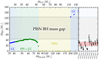 |
Fig. 2. Final BH masses as a function of the initial He core mass. The scale in the horizontal direction is logarithmic. The colors in the background indicate the approximate range for each evolutionary path, see also Sect. 3. Right panel: masses inferred from the first ten binary BH mergers detected by LIGO/Virgo, with a red shade to emphasize the overlap between PPI and CC, and green and blue hatches to indicate the fate of the progenitor in different BH mass ranges. |
The colored background in the left panel of Fig. 2 indicates approximately the evolutionary path for the corresponding mass range. The four possibilities are summarized as follows, in order of increasing initial He core mass:
CC. Relatively low mass He cores end their lives in a core collapse (CC, blue on the left of Fig. 2) event without losing mass to pair-production driven pulses. For these models, the layers which are unstable to pair production (if any) are not massive enough to cause an episode of mass ejection. In this mass range, the outcome of core-collapse is most likely BH formation, possibly associated with a weak SN with large fallback (Ott et al. 2018; Kuroda et al. 2018; Chan et al. 2018, 2020). We return on the “explodability” of our grid of models in Sect. 7.
PPI+CC. With increasing MHe, init, the pair instability becomes progressively more violent. The energy release by thermonuclear explosions causes significant radial expansion. Increasing further in mass, models experience one or more mass loss episodes, before the core is stabilized by the consumption of fuel and entropy losses to neutrinos, and the stars finally collapse (PPI+CC, green in Fig. 2).
PISN. For 80 M⊙ ≲ MHe, init ≲ 200 M⊙, our models are completely disrupted in a PISN, and produce no remnant (yellow vertical area in Fig. 2). Our lowest mass model going PISN and leaving no remnant has MHe, init = 80.75 M⊙, corresponding to a maximum CO core mass of ∼55 M⊙ (see also Farmer et al. 2019).
CC. For extremely massive cores, MHe, init ≳ 200 M⊙, the energy release by the explosive thermonuclear burning triggered by the pair instability is insufficient to fully disrupt the star. This happens because most of that energy is used to photodisintegrate the nuclear ashes and lost to neutrinos, instead of becoming kinetic energy of the stellar gas (Bond et al. 1984; Fryer et al. 2001). Therefore, models above a certain threshold reach CC without any PPI-driven mass loss (blue area on the right of the panel of Fig. 2).
In Fig. 2 the transition between the CC and PPI+CC is smooth, and we have avoided quantifying the boundary between the low mass CC and PPI+CC because of the subtleties in the definition of “pulse”. We outline three physically motivated definitions, each one shifting the CC/PPI+CC boundary, in Sect. 5.
4. Resulting BH masses
The PISN BH mass gap is denoted by the hatched region in the left panel of Fig. 2. The lower and upper edge of the gap can be read from the y-axis. With our numerical setup, we find a maximum BH mass below the PISN gap of max{MBH}≃45 M⊙, in good agreement with the lower boundary of the gap from previous studies Woosley (2017, 2019); Marchant et al. (2019), Leung et al. (2019), Farmer et al. (2019). At the upper-end, the PISN BH mass gap is closed by the photodisintegration instability causing the direct collapse of an initially MHe, init = 200 M⊙ He core, which builds up a CO core of MCO ≃ 114 M⊙ and eventually forms to a BH of 125 M⊙. This value corresponds very closely to the final He core mass of this model, after wind mass loss. This upper boundary too is in good agreement with the results from Woosley et al. (2002), Woosley (2017), although it is sensitive to the metallicity and uncertainties in the wind mass loss rate.
We do not expect these boundaries would have varied if our models had a H-rich envelope (e.g., Woosley 2017), especially if the progenitor stars evolve in close binaries which can remove the H-rich envelope long before the PPI. The combination of the mass loss (Ott et al. 2018; Kuroda et al. 2018; Chan et al. 2018, 2020) and energy loss to neutrinos at BH formation (e.g., Coughlin et al. 2018) should be sufficient to unbind any the residual H envelope, unless the progenitor is a blue super giant with a large binding energy of the envelope (exceeding ∼1048 erg, Lovegrove & Woosley 2013). Such blue supergiant pre-PPI structures might arise from binary mergers (e.g., Spera et al. 2019, for a population synthesis study). However, the stellar structure calculations for the merger of two post-main-sequence stars from Vigna-Gómez et al. (2019) show extended convective envelopes at the onset of the instability, which support our expectation that the envelope would easily be shed at the onset of the instability (see also Appendix B). Whether the H-rich envelope can contribute to the BH mass or not deserves further investigation.
The right panel of Fig. 2 shows for comparison the individual BH masses of the binary BH mergers detected to date by LIGO/Virgo6, with the 90% confidence level uncertainty ranges. The masses of the two BHs in a merger event are not direct observables, they are instead inferred from the chirp mass and total mass of the binary. The color of the hatching in the right panel indicates the possible progenitor evolution (see also Sect. 3): the red area emphasize the range of BH masses that can be obtained by CC of a lower mass model, or by severe PPI mass loss of the most massive PPI+CC models. Its extent to the lower BH masses is somewhat dependent on the resolution in MHe, init of our grid. However, in Marchant et al. (2019) we showed that the minimum BH mass that can be obtained by PPI+CC evolution is about 10 M⊙ because of the production of radioactive material that can unbind cores that recover hydrostatic equilibrium of lower masses. Most BH progenitors for the gravitational wave mergers events detected to date are compatible with encountering the PPI, although we do not expect most of them to have gone through this evolution because progenitors with sufficient mass are disfavored by the initial mass function.
5. The physics of pulses: cores, radii, and mass ejections
While the nuclear and thermal processes governing the evolution of a star through pair instability are well understood, the characterization of the observable properties of such events are not yet as clear. The main reason for this is that stars do not react “elastically” to the pair instability: instead the nuclear binding energy released by burning episodes at each pulse is stored and re-distributed throughout the stellar structure, and there is not a one-to-one correspondence between what happens in the core and what can be observed at the surface.
To clarify the distinction between core behavior and observable properties from the outermost layers of the star, in this section we describe the physical processes that can be used to give three different physically-motivated definitions of “pulse”, and illustrate them with an example MHe, init = 50 M⊙ He core (for which we also present a resolution study in Appendix A). These definitions do not cover all the possible ways in which pulses can be defined and counted. For example, Woosley et al. 2007; Woosley 2017 uses the core temperature Tc while in Marchant et al. 2019 we adopted a criterion based on the maximum velocity in the stellar interior.
5.1. Thermonuclear ignition
Historically, studies on pair-instability evolution have focused on the core of stars. Indeed, the region that becomes unstable because of the runaway production of e± is typically deep in the star, and the subsequent evolution is driven by the explosive burning of oxygen and heavier fuel (e.g., Barkat et al. 1967; Rakavy & Shaviv 1967; Fraley 1968; Woosley et al. 2007; Woosley 2017; Marchant et al. 2019; Leung et al. 2019). This allows for a definition of a pulse based on the behavior of the deep interior of the star.
Figure 3 shows the evolution of the central temperature (Tc, bottom panel) and nuclear and neutrino luminosity (Lnuc and Lν respectively, top panel) during the last year before CC for a MHe, init = 50 M⊙ He core. The horizontal axis shows the time to the onset of CC on a reversed logarithmic scale.
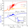 |
Fig. 3. Last year of evolution of the central temperature (blue, bottom panel), nuclear (red) and neutrino (orange) luminosity (top panel) for a 50 M⊙ He core. The inset in the bottom panel shows the readjustment of the core to hydrostatic equilibrium after the first pulse, which we resolve even if this behavior is likely to be influenced by the imposed spherical geometry. |
During the previous evolution (not shown), this model is thermally and dynamically stable. At log10{(tCC − t)/[yr]} ≃ 2, the core becomes thermally unstable because of the softening of the EOS, causing the collapse of the core and rise in Tc allowing for the explosive ignition of fuel. The latter can be seen as spikes in the nuclear luminosity Lnuc. The thermonuclear release of energy expands the core, cooling it adiabatically and causing a temperature drop. Eventually, the core is stabilized by the loss of entropy to neutrinos and the burning of nuclear fuel, and it ends its life steadily increasing its core temperature until the onset of CC.
If we define PPI pulses based on core temperature spikes, or equivalently spikes in nuclear and neutrino luminosity, then the lowest mass He core showing hints of pulsational behavior is MHe, init ≃ 37.5 M⊙, corresponding to a final MCO ≃ 28 M⊙. Even if the local adiabatic index Γ1 < 4/3 somewhere in this model, the volumetric pressure-weighted averaged adiabatic index is always ⟨Γ1⟩> 4/3 for the entire evolution. The thermonuclear ignition in the core never results in a global instability of the star. We find that ⟨Γ1⟩ crosses the stability threshold of 4/3 at some point in the evolution only for MHe, init > 40.5 M⊙.
The inset plot in the bottom panel of Fig. 3 shows that in a one-dimensional spherical MESA model the core “bounces” off itself, which was already noted in Paxton et al. (2018). These readjustments of the core cause secondary burning episodes (Renzo et al. 2020) which can release further energy and introduce complications in counting the Tc spikes (see also Marchant et al. 2019). While we resolve in time these bounces by taking timesteps shorter than the dynamical timescale of the core, it is likely that multidimensional effects and/or off-center energy release would affect them significantly. Even counting the core oscillations as one individual pulse, our MHe, init = 50 M⊙ model exhibits tens of thermonuclear-ignition pulses.
This behavior of the core of very massive stars encountering the pair instability is well established (e.g., Barkat et al. 1967; Woosley 2017; Marchant et al. 2019; Leung et al. 2019). However, since these processes happens deep inside the optically thick layers of the star, their only direct observable is the rapid variation of orders of magnitude of the neutrino luminosity during each pulse (Fryer et al. 2001, and possibly during the post-pulse bounces). However, because of the rarity of such massive stars in the local Universe, such variations in the neutrino luminosity are unlikely to be easily observed.
5.2. Radial expansion
In Sect. 5.1 we discussed a definition of a PPI pulse based on the thermonuclear behavior deep inside the core. However, for MHe, init > 41 M⊙, the nuclear binding energy released by the thermonuclear explosions deep down can have an observable impact on the surface of the star. We emphasize that either because of other evolutionary processes, or because of a previous PPI mass-loss episode, the surface can be a He rich layer for these stars. Therefore, we can use our He core models to define a PPI pulse based on surface properties, assuming the H-rich layers have been lost before.
The thermonuclear burning injects energy into the core and drives a pulse wave, which propagates down the decreasing density profile of the star and eventually steepens into a shock. The core, post-explosion, readjusts and can contribute to driving secondary shocks. There is a small range in mass, 41 M⊙ ≲ MHe, init ≲ 42 M⊙ in which these shocks, which can often catch up with each other below the stellar surface, are not energetic enough to dynamically unbind any significant amount of matter (see also Sect. 5.3). Nevertheless, even in this mass range, they produce a potentially observable radial expansion of the star. For models more massive than MHe, init ≳ 42 M⊙, the energy released in the thermonuclear explosion also cause the ejection of material (see Sect. 5.3).
Figure 4 shows the radial evolution of our 50 M⊙ example. The orange line shows the photospheric radius (defined as the location where the optical depth is 2/3). For most of the evolution in hydrostatic equilibrium (until tCC − t ≃ 10−2 years), the stellar radius is on the order of the solar radius (R⊙ ≃ 6.9 × 1010 cm) or less. As the star contracts and approaches the instability, we switch to the HLLC solver at around tCC − t ≲ 1 year, when the thicker red line appears in Fig. 4. This line shows the radius of the bound material R(v < vesc) and is plotted only when the hydrodynamics is on.
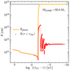 |
Fig. 4. Radial evolution of a Minit = 50 M⊙ He core through PPI pulses. The radius of the bound material (red, plotted only during dynamical phases) oscillates because of the PPI. The photospheric radius (orange) reaches 104 R⊙ (dashed line) during the dynamical phase of evolution, i.e., the location at optical depth 2/3 is in the material already ejected. |
We follow the thermal contraction of the star due to the pair instability, and at tCC − t ≃ 10−2 years a shock wave propagating from the core causes a radial expansion by two orders of magnitude on a dynamical timescale. The material remaining bound to the star extends to ∼1013 cm. For our MHe, init = 50 M⊙ model, the pulse also ejects matter and the ejected layer extends beyond 1014 cm. For numerical stability reasons we cap the radii at 104 R⊙ ≃ 6.9 × 1014 cm (horizontal dashed line in Fig. 4), and treat this limit as an open boundary7. We discuss the ejected matter more extensively in Sect. 5.3.
The ejected layer can obscure the bound surface of the star: the location where the optical depth is 2/3 extends all the way to the outermost layers of our Lagrangian mesh. However, we emphasize that the structure of the material moving faster than the escape velocity should be recomputed accounting for radiative losses for a better determination of the photosphere. It is possible that such stars would exhibit large radius differences at different wavelengths, with some that might even appear red during their maximal radial expansion. For this particular model, the photospheric radius does not have time to recover its prepulse value, since the radial expansion only started days before the final core-collapse. More massive models have more violent pulses that drive the inner core farther out of thermal equilibrium and for which it takes longer to recover the condition for further (explosive or stable) nuclear burning (see also Sect. 6): this can give time to the photospheric radius to decrease again.
The bound radius instead experiences large oscillations between 1011 cm and 1013 cm (the maximal expansion reached initially). In this case, these might not be directly obervable since they are embedded within the pseudo photosphere of the ejecta. Models more massive than our example might have rather long lived phases with large radii, which might have implications for binary interactions (e.g., Marchant et al. 2019) and wind mass loss physics.
5.3. Ejection of material
Although the two definitions of a pulse we introduced in the previous subsections (based on the core explosive behavior and on the radial expansion, respectively) might possibly give observable “pulses”, the processes they are based on do not leave a direct imprint on the CSM structure, nor on the remnant BH mass. Observational confirmation of the occurrence in nature of PPI+CC evolution (and possibly PISN) is most likely to come from either observations of transients which can probe the CSM around the exploding star and/or the distribution of BH masses probed through gravitational waves. It is therefore worth giving a definition of pulse based on the nonterminal ejection of material from the stars: the ejecta carry away mass, decreasing the final BH mass and shaping the CSM structure.
Our simulations produce output for the ejecta at each timestep. The top panel of Fig. 5 shows the cumulative mass lost to PPI-driven pulses for our example MHe, init = 50 M⊙ He core. In this specific model, the total (H-free) ejecta mass is about 1.2 M⊙ by the end of the evolution. Had our star retained an H-rich envelope until the onset of the first pulse, the remaining H-rich envelope at the onset of the instability would likely add to the amount of mass in the CSM (see also Appendix B).
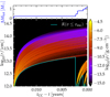 |
Fig. 5. Space-time diagram for propagation of the PPI ejecta of a 50 M⊙ He core. The color indicates the density, assuming radial expansion at constant velocity. The top panel indicates the cumulative amout of ejected at velocities larger than the escape velocity through pulses only (i.e., excluding the wind mass loss). The cyan curve shows the radius of the material instantaneously bound (cf. the red curve in Fig. 4). |
The bottom panel of Fig. 5 shows the density distribution around the star as a function of distance from the star (y-axis) and time until the final CC (x-axis). The cyan line shows the radius of the bound material (cf. the red curve in Fig. 4), which we assume to be the initial radius from which the ejecta are launched. To compute the CSM density we assume propagation of the ejecta at constant velocity. We use the velocity at the time the material first exceeds the local escape velocity as computed by MESA, and it is typically a few thousand km s−1. We return to the ejecta velocity in Sect. 6. Assuming a constant velocity for the propagation of the ejecta corresponds to neglecting radiative cooling, internal collisions of the ejecta, and multi-dimensional effects (e.g., Chen & Woosley 2020), and we discuss it here only for illustration purposes. Our output files8 contain the amount of mass ejected, its center-of-mass velocity, chemical composition and thermal state (averaged by mass over all the mesh points that exceed the local escape velocity in the current timestep), which could be used as input for more detailed simulations to predict the CSM structure around PPI+CC models. This ejecta output neglects the possibility of fallback, which however could be implemented when using these files as input for hydrodynamical simulations of the CSM.
The CSM structure shown in Fig. 5 for our example model shows H-poor/He-rich CSM starting from ∼1013 cm and extending out to ∼1014 cm. The CSM densities reach 10−5 − 10−4 g cm−3. These value are typical for the models in our grid, and fall in the range of CSM distances and densities inferred from transient observations (e.g., Gomez et al. 2019).
However, mass ejections that happen in subsequent timesteps (possibly with no mass ejected in between) in MESA might not be physically distinct events. To count the mass-ejection events, we need to group mass ejections in timesteps separated by less than a dynamical timescale in one individual event. Moreover, one mass ejection event can last several dynamical timescales, for example the final mass ejection and full disruption of a PISN is expected to produce a long transient (e.g., Gal-Yam et al. 2009). We estimate the dynamical timescale as the free-fall timescale  where G is Newton’s constant, and Rphoto and Mbound are the (time-dependent) photospheric radius and mass gravitationally bound to the star. We define the beginning of a mass loss event as the timestep during which at least 10−6 M⊙ has been removed from the star since the last mass loss event (either in one timestep, or cumulatively). We require each mass ejection event to last at least one free fall timescale (calculated at the beginning of the pulse), and define its end as soon as the amount of mass to be ejected in the following 100 τff (now calculated at the end of the pulse) is less than 10−7 M⊙. This last condition allows us to count as a single event mass ejection episodes that last longer than a dynamical timescale. All together, these requirements enforce that ejections which numerically happen in different timesteps separated by less than a free fall timescale are not counted as separate events.
Adopting this criterion to count the mass ejection events, our MHe, init = 50 M⊙ model only has one mass-ejection episode (cf. tens of core ignitions, see Sect. 5.1), which starts roughly ∼0.015 years ≃ 130 h before CC.
We can tentatively apply the same threshold to define the beginning of an explosion for a terminal PISN with full disruption. In this case, the duration of the PISN events in our grid exceeds months even for the least massive PISN model with MHe, init = 80.75 M⊙ in agreement with previous studies. Our stopping conditions do not allow models to reach what would appear as the observational end of a PISN.
6. Pulsational pair-instability-generated CSM
We now discus the CSM that can be created by PPI evolution across our grid of models. In principle, this CSM can be probed by time-domain observations, if the final core-collapse causes an associated explosion (see Sect. 7), or because of collisions between shells ejected at different times (e.g., Woosley et al. 2007; Woosley 2017, 2019). Most of the CSM properties do not depend on which criterion is used to define the beginning or end of the pulses, except the number of pulses and their duration. For these quantities, we adopt the definition of Sect. 5.3 based on the ejection of matter, which is the most relevant for discussing the CSM structure.
Table C.1 summarizes the time, duration, and amount of mass loss in each event for all the PPI+CC models in our grid, and Fig. 6 shows the number of pulses as mass-ejection events contributing to the CSM. Models evolving to CC without any mass ejection have zero pulses. We define full disruption in a PISN as a one-pulse event, although these would not contribute to the CSM itself. The color in the background emphasizes the various evolutionary behaviors, but using the definition from Sect. 5.3 the mass threshold separating CC (blue) from PPI+CC (green) evolution is well defined at MHe, init = 40.5 M⊙, correponding to MCO = 30 M⊙.
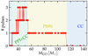 |
Fig. 6. Number of mass-ejection events caused by pair instability as a function of CO core mass. The color shading indicates the approximate range for each behavior: core collapse without experiencing PPI-driven mass loss (CC, blue), PPI-driven mass loss (PPI+CC, green), or full disruption in a PISN (yellow), which we define as one mass loss event. The noisiness is caused by the occurrence of mass loss event right at the time of the final core collapse. |
The number of pulses is zero at the lower end, and increases up to three distinct mass-ejection events for the central part of the PPI+CC mass range. At even higher masses, approaching the PPI+CC/PISN boundary, the number of pulses decreases again, although the amount of mass ejected increases (see also Fig. 8): this is because pulses become more energetic and consume more nuclear fuel at once (e.g., Woosley et al. 2007; Chatzopoulos & Wheeler 2012b; Woosley 2017, 2019).
The green region shows some noise in the number of pulses: the reason for this is illustrated in Fig. 7, which shows the velocity as a function of Lagrangian mass coordinate for our MHe, init = 50 M⊙ core at the onset of core collapse. Many models exhibit a similar behavior, with an outgoing pulse wave at the onset of CC: this means that the PPI mass ejection is still going on while the Fe core starts collapsing.
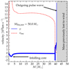 |
Fig. 7. Velocity profile at the onset of core-collapse for a 50 M⊙ He core, which undergoes a PPI mass-loss event while collapsing. The dashed red line shows the escape velocity profile, the thick blue line indicates the profile of the bound material, while the thinner line represents material still on the Lagrangian mass grid, but already beyond the escape velocity. The gray area indicates the model dependent amount of mass lost to stellar winds. |
Figure 8 summarizes the amount of mass lost to PPI-driven pulses across our model grid. The bottom panel shows the amount of mass lost per individual pulse, the pulse number is represented by the color of the filled circles.
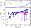 |
Fig. 8. PPI-driven mass loss as a function of the CO core mass. Top panel: total mass ejected in pulses, bottom panel: mass lost in individual pulses. The amount of mass lost does not have a monotonic behavior with pulse number, and spans a wide range of values. The first pulse is shown as a blue dot, and the second and third, if they occur, are shown as a purple plus and red cross, respectively. Thin vertical lines connect multiple pulses for the same MCO. |
The typical amount of mass lost varies from ≲10−3 M⊙ for the lowest-mass models ejecting some mass, up to ≃20 M⊙ (of He-rich material) at the upper mass end, just below the minimum mass for PISN. For models producing more than one mass ejection event (i.e., the models for which also a purple and possibly a red dot are shown), the amount of mass lost per pulse does not behave monotonically with the pulse number. For 50 M⊙ ≲ MHe, init ≲ 62 M⊙, corresponding to 36 M⊙ ≲ MCO ≲ 43 M⊙ the second pulse (purple) ejects more mass than the first (blue), while for higher masses the first pulse removes more mass than the second.
The top panel of Fig. 8 shows the total amount of mass lost to PPI ejecta, i.e., the sum of the mass ejected in each individual pulse. A trend of more massive models producing more energetic pulses and driving more mass loss is evident. We provide a simple fitting formula for the total amount of He-rich mass lost in PPI-driven events for 33 M⊙ ≤ MCO ≤ 56.5 M⊙ which produce a CSM mass larger than ∼0.2 M⊙, shown as a dashed gray line in the top panel of Fig. 8:
 (2)
(2)
The total mass lost to pulses should be added to the amount of mass lost due to winds to calculate the total mass in the CSM. The density distribution of the CSM generated by PPI-driven pulses and wind mass loss are likely to be very different from each other. In cases where stars retain a (loosely bound) H-rich envelope at the onset of the first pulse, the mass of such an envelope at the start of the pulses should also be added to the total mass lost in the first mass loss event.
Figure 9 shows the delay time between the end times mass ejections and the final CC, as a function of the CO core mass of our models. The timing of the mass-loss events also spans a large range, from zero (see also Fig. 7 for example) to ∼104 years, corresponding roughly to the Kelvin-Helmholtz timescale of the most massive PPI+CC. We emphasize that many models in our grid show submonth delays between the last pulse and the final CC, which makes them candidates for the detection of CSM interactions in early observations of the SN explosions (see also inset in Fig. 9).
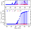 |
Fig. 9. Delay time between the final core-collapse and the end of each mass loss event in a PPI pulse. Typical delays are on the order of few months, but they increase steeply with the initial He core mass of the PPI progenitor, which produce fewer but more energetic pulses, up to 104 years. The top inset magnifies the range of half a year delays on a days scale. The first pulse is shown as a blue dot, and the second and third, if occurring, are shown as a purple plus and red cross, respectively, with a thin blue line connecting the pulses of the same model. |
The delay (in between pulses and between each pulse and CC) increases with the core mass, because more massive models produce more energetic pulses that drive the star farther from gravo-thermal equilibrium, increasing the amount of time needed to return to equilibrium after a pulse and resume the final evolution. While typically for very massive stars the neutrino luminosity greatly exceeds their photon luminosity Lν ≫ L (they are “neutrino stars”, Fraley 1968), this is not always true for the most massive PPI+CC models. For these, the adiabatic expansion of the core can leads to central temperature and densities too low for significant neutrino cooling to occur. Thus, after a pulse begins, these models transition from evolving on a neutrino-mediated thermal timescale (∝GM2/RLν) to a photon-mediated thermal timescale (∝GM2/RL) in between pulses, which increases their interpulse time.
Figure 10 shows the center-of-mass velocity of the layers ejected (which is calculated as the mass-weighted average of the center-of-mass velocity of the layers ejected at each timestep over the duration of the mass ejection event). Unlike the other quantities characterizing a pulse, the ejecta velocities we find do not span orders of magnitude, and are typically a few ∼1000 km s−1. This suggests that mass ejection during a PPI might explain the He-rich circumstellar material required to explain at least some of the spectra of SN Ibn showing narrow He emission lines (e.g., Pastorello et al. 2008), provided that there is a way to excite the ejected shells. This could be due to collisions between the third and second pulse within the first ejected shell, or because of a successful explosion at the final CC (see also Sect. 7).
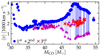 |
Fig. 10. Center-of-mass velocity of the layers ejected at each pulse. The first pulse (blue filled circles) produces typically higher ejection velocities, and the ejecta move at ∼ few thousand km s−1 which suggests a connection with (some subclasses) of SN Ibn. |
The first pulse (blue filled circles) are almost always faster than the later pulses. Conversely, when they occur, the third pulse (red crosses) is often faster than the second (purple pluses). Therefore, many models might result in collisions in between the ejecta which can appear as SN impostors, as noted by Woosley et al. (2007) and Woosley (2017).
We only report the center-of-mass velocity for the ejected shells, because our treatment of the ejecta is presently very simplified. Radiation-hydrodynamics simulations of the ejecta propagation would be desirable to properly quantify the velocity distribution of the ejecta, and in particular quantify the low-velocity tail which will appear first in observations of CSM interactions.
7. Explodability of CC and PPI+CC models
Does the final CC of a post-PPI star result in a successful explosion? This question remains relevant because a terminal explosion would potentially allow us to probe all the layers ejected previously. Whether the final collapse of PPI+CC evolution is accompanied by a successful, albeit possibly weak, explosion likely constitutes the biggest uncertainty underlying this study, and it is not a question that we can settle using only our stellar structure models. We emphasize that even in the absence of a terminal explosion, electromagnetic transients from PPI are possible and expected because of collisions between shells (e.g., Woosley et al. 2007; Woosley 2017, 2019, and Sect. 6).
Based on the extrapolation of one-dimensional parametric CC simulations, the typical expectation is that He cores with masses larger than ≳10 M⊙ fail to explode (e.g., O’Connor & Ott 2011; Ugliano et al. 2012; Ertl et al. 2016), therefore a successful terminal explosion in PPI+CC models appears unlikely. However, the observations of (BH) X-ray binary kinematics (e.g., Brandt et al. 1995; Fragos et al. 2009; Atri et al. 2019, and references therein), and possible spin misalignment in gravitational wave events (e.g., O’Shaughnessy et al. 2017) might require BH natal kicks. These can occur only with an explosion and some level of asymmetry in the ejecta (e.g., Janka 2013, 2017; Chan et al. 2018, 2020, or possibly in the neutrino flux). Thus, the current understanding of BH formation cannot yet be considered final.
As far as we are aware, there are no published multi-dimensional calculations investigating the final “explodability” of PPI+CC structures. Most of the available studies (e.g., Ott et al. 2018; Kuroda et al. 2018) target much lower mass progenitors (up to ∼70 M⊙ including the H-rich envelope) and/or rely on artificially imposed large perturbations or enhanced neutrino-nucleon scattering to obtain explosions (e.g., Chan et al. 2018, 2020). Therefore, these results may not meaningfully extrapolate to the PPI+CC regime.
Even in the case of successful but weak explosions, these studies either do not follow the explosion long enough to study the amount of mass ejected (if any), or find that only a fraction of the envelope is ejected (e.g., Chan et al. 2020). While our models do not have any H-rich envelope to begin with, the He core at precollapse can reach radii similar to that of a H-envelope in yellow-supergiant stars. Specifically, the radii of bound material (v < vesc) at the onset of CC range between a few to a few hundreds of solar radii (∼1011 − 1013 cm). Such extended He cores, effectively akin to He envelopes in some cases, have significantly different density profiles compared to the stellar structures explored in the aforementioned studies. It is unclear whether the usual definition of the core-envelope boundary, based on abundances, makes sense from a core-collapse dynamics perspective for our models.
Although also unexplored and uncertain in this regime, even very weak explosions due to the initial neutrino emission before the formation of an event horizon (e.g., Nadezhin 1980; Lovegrove & Woosley 2013; Coughlin et al. 2018 and possibly observed by Adams et al. 2017) might potentially be sufficient to start an electromagnetic transient when the outermost layers hit the previously ejected mass. Once again, this mechanism is thought to only eject loosely-bound H-rich outer layers at low velocity, and in red supergiant progenitors of much lower mass than we explore here. The large radial extension of some of our precollapse models might possibly result in the ejection of some equally loosely bound material, but the typical amount of mass with binding energy sufficiently low is only of order 0.01 M⊙. Should this scenario produce some ejecta, the amount of kinetic energy available seems unlikely to produce transients detectable at large distances (Chevalier & Irwin 2012).
Explosion mechanisms relying on rotational energy (e.g., Mösta et al. 2015) and jets (e.g., Gilkis et al. 2016; Soker 2019), which have also been proposed to explain type Ic SNe showing broad lines (e.g., Barnes et al. 2018) might also deserve attention in this context. In Marchant et al. (2019) we showed that PPI-driven mass loss does not dramatically decrease the core angular momentum. However, we are not aware of any “explodability” criterion for this kind of core-collapse engine.
One key difference between PPI+CC cores and lower mass stars contributing to the differences in density profiles is the production of 56Ni during pulses, before the final CC. We emphasize that the energy released by 56Ni decay is not expected to play a role during core-collapse, as the half-life of 56Ni is much longer than the few hundred millisecond timescale of CC. Its effect is to modify the initial conditions for CC during the interpulse evolution of the models.
The typical outermost mass coordinate where we find a mass fraction of 56Ni larger than 0.01 is less than 5 M⊙, thus we expect most of the 56Ni will eventually be accreted into the final BH. However, the 56Ni is produced weeks, months, or up to several years before CC. This provides sufficient time for the 56Ni to decay and causes the core to expand due to this heating. This makes the precollapse core structure of PPI+CC models qualitatively different from lower mass models routinely used for CC simulations. Detailed simulations of the final CC structure (including large nuclear networks to capture the precollapse deleptonization, Farmer et al. 2016; Renzo et al. 2017) and explosion are needed to shed light on what the qualitative differences mean for the “explodability” of PPI+CC models. In the most massive PPI+CC models, the decay of the 56Ni produced during pulses can ultimately unbind what is left of the core resulting in a minimum BH mass that can be obtained via PPI+CC (see also Marchant et al. 2019).
Figure 11 shows the amount of 56Ni present in our PPI+CC and PISN models at the end of the evolution: for PPI+CC models the total mass of 56Ni is typically MNi ≃ 0.2−0.4 M⊙, i.e., about one order of magnitude more than what is produced in typical core-collapse SNe (e.g., Wongwathanarat et al. 2013). This value increases steeply in the PISN range, reaching about ∼60 M⊙ at the upper end, in good agreement with Heger & Woosley (2002) and Woosley et al. (2002) results. However, our calculations are based on a 22-isotope nuclear reaction network which is known to produce MNi deviating by up to a factor of ∼1.5× in either direction from results computed with larger nuclear reaction networks (regardless of the final fate of the models between CC, PPI+CC, or PISN).
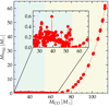 |
Fig. 11. 56Ni mass present in the deep interior of the star at the onset of CC or PISN. The color background is the same as Fig. 6 and indicates the approximate evolution (CC for blue, PPI+CC for green, and PISN for yellow). We computed these models using a 22-isotope nuclear reaction network. |
Table 1 lists, for a representative subset of models, quantities commonly used to determine the “explodability” of a stellar model. These focus on the innermost layers of the star, but already include the effect of the precollapse decay of 56Ni produced during pulses in this region of the star. Specifically, we report the initial He core mass MHe, init and its value at the end of He core burning9MHe, depl, the CO core mass MCO, the final iron core mass MFe, defined as the outermost location where the mass fraction of 28Si ≤ 0.01 and the mass fraction of Fe-group elements, i.e., with more than 46 nucleons, exceeds 0.1; and the two parameters proposed by Ertl et al. (2016). These are the mass coordinate M4 at which the specific entropy reaches 4kBNA, where kB is Boltzmann’s constant and NA is Avogadro’s number, and the mass gradient at this location μ4 (Eq. (6) in Ertl et al. 2016). Since the nuclear reaction network we employ does not allow for detailed treatment of the electron captures and β decays, which determine the final electron-to-baryon ratio, we avoid listing the compactness parameter (e.g., O’Connor & Ott 2011), which is sensitive to these modeling assumptions (Farmer et al. 2016; Renzo et al. 2017). We caution that three-dimensional simulations (e.g., Ott et al. 2018; Kuroda et al. 2018; Chan et al. 2018, 2020) might give a different outcome than 1D parametric simulations used to assess the explodability of grids of models (e.g., O’Connor & Ott 2011; Ugliano et al. 2012; Müller 2019; Couch et al. 2019).
He core mass at the beginning of our simulations (MHe, init) and at He depletion (MHe, depl), carbon-oxygen core mass (MCO), iron core mass (MFe), mass location M4 where the specific entropy is lower than 4kBNA, and mass gradient μ4 ≡ dM/dr|s = 4kBNA for a representative subset of our models eventually forming a BH at Z = 0.001.
The iron core mass is typically below ∼2.5 M⊙ below the PISN BH mass gap. The values for models above the PISN BH mass gap are sensitive to the amount of nuclear burning going on before the stopping criterion based on the infall velocity is reached, and because of their large mass, the entropy is larger than 4kBNA throughout these stars. Because of the as of yet insufficient understanding of black hole formation it is hard to predict whether these models would give a successful, albeit possibly weak, explosion. We would expect that if successful explosion can happen, they would be powered by fallback accretion.
Figure 12 shows our CC (blue) and PPI+CC (green) on the plane used by Ertl et al. (2016) to determine the “explodability”. They determine it using 1D parametric simulations aiming at reproducing SN1987A starting with single star progenitors of initial mass 15−20 M⊙. The red area indicates the region where some of their engines produce explosions and neutron star formation, while others produce failed explosions and BHs (see their Table 2 and Fig. 8). Above this (gray area), Ertl et al. (2016) predict BH formation with a failed explosion, while below they predict successful explosions with neutron star formation. Applying this criterion to our models requires extrapolating significantly outside the range originally explored by Ertl et al. (2016), shown by the dotted rectangle in the bottom left corner. We omit from the plot the models models above the PISN BH mass gap in our grid for which M4 and μ4 are zero. Most of our PPI+CC models fall in the failed explosion region according to the Ertl et al. (2016) criterion. A few enter in the region that depends on the assumed calibration for their model, and some cross marginally into the successful explosion and neutron star formation region. The more explodable models correspond to lower initial He core masses, but there is a large scatter in the trend. All of our CC models fall in the region for BH formation without an explosion.
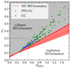 |
Fig. 12. CC and PPI+CC models on the Ertl criterion plane for “explodability”. The red area indicates the uncertain boundary region between successful explosions and neutron star formation (white) and collapse with BH formation (gray). The dotted rectangle in the bottom left indicates the range originally showed in Ertl et al. (2016), most of our models require extrapolating outside this range. Blue dots correspond to CC models, while green dots show PPI+CC models. |
Figure 13 shows the surface mass fractions of 4He, 12C, 16O at the onset of core collapse for our CC and PPI+CC models. Should the CSM evolve to be (partially) optically thin at the time of the final CC and in case this results in a successful explosion, the surface composition of the star and the mixing processes (e.g., Dessart et al. 2012) would determine the spectral type of the SN. Most PPI+CC models experiencing a significant amount of mass loss show He-poor surfaces, and enhanced carbon (and to a smaller extent) oxygen mass fractions, corresponding to type Ic SNe. Because of the radial expansion caused by the pulses, some of these progenitors might look like extended and cool objects at the onset of collapse, rather than compact and hot progenitors. Conversely, if the He-rich CSM is optically thick, it might obscure the progenitor star and the embedded explosion, and we expect that re-processing of the photons by the shell would produce He lines (possibly narrow and in emission) corresponding to a type Ib(n) SN.
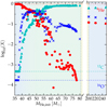 |
Fig. 13. Surface composition at the onset of core-collapse for the PPI+CC and CC models. 4He, 12C, 16O are shown as red filled circles, cyan triangles, and blue crosses, respectively. The dot-dashed horizontal lines of the same color mark the initial mass fraction for these elements for our Z = 0.001 model grid. The colored background indicates the approximate evolution of the star (cf. Fig. 2 and Sect. 3). |
We omit from Fig. 13 the PISN models because our stopping condition for these conservatively ensures the full star is unbound, but it might not correspond to the “beginning” of the explosion. Nevertheless, most PISN models start exploding while still retaining some He at their surface (corresponding again to type Ib SNe) with the wind mass-loss rates and metallicity adopted here.
Figure 13 also shows a trend with the initial He core mass: the larger the initial MHe, init, the more mass is lost to winds and PPI, the lower the surface He mass fraction and the higher the carbon and oxygen mass fractions. In the mass range 50 M⊙ ≲ MHe, init ≲ 75 M⊙, corresponding roughly to the region where we find three distinct PPI-driven mass loss events, the predicted surface abundances appear more noisy.
8. Comparison to selected supernovae
Stars experiencing the PPI+CC evolution should intrinsically be rare because of the large initial mass necessary to build up a sufficiently massive core. To produce a significant amount of CSM via PPI-driven pulses, our results suggest that the He core mass needs to initially exceed MHe, init ≳ 42 M⊙, corresponding to MCO ≳ 31 M⊙. Therefore, the rate of observed transients that can be interpreted as signatures of PPI evolution should be small. Possibly for this reason an unambiguous detection of PPI+CC/PISN in time-domain surveys is not yet available, although the physical mechanism underlying this phenomenon is well understood. We consider here a few notable and recent H-less type I SNe that have been proposed as PPI+CC candidates.
PTF12dam. Tolstov et al. (2017) modeled the H-less (type I) superluminous supernova PTF12dam as powered by the combination of 56Ni decay and CSM interaction. They proposed that combination of energy sources invoking the following scenario: first the H-rich envelope is removed by stellar winds, then the PPI pulses produce ∼20−40 M⊙ of CSM before the final CC synthesizes and ejects M56Ni ≃ 6 M⊙ of radioactive material. Our results, albeit computed with a small nuclear reaction network, never produce this combination of CSM mass and M56Ni: PPI ejecta exceeding 20 M⊙ are found only for MHe, init ≳ 75 M⊙ or equivalently MCO ≳ 51 M⊙ (cf. Fig. 8), and only about ∼0.2 M⊙ of 56Ni is synthesized for PPI+CC models. Assuming that the final CC proceeds similarly as for lower mass stars, we expect it would add ∼0.03–0.05 M⊙ of 56Ni (e.g., Wongwathanarat et al. 2013), which does not help to reach the M56Ni claimed. An initial He core mass exceeding MHe, init ≳ 140 M⊙, or MCO ≳ 87 M⊙, is required to reach the amount of radioactive material required by Tolstov et al. (2017), which would put the model in the PISN range where we do not expect CSM from PPI.
iPTF16eh. Lunnan et al. (2018) detected a time and frequency varying MgII line in the spectrum of the type I superluminous supernova iPTF16eh. They interpreted it as a light-echo of the explosion bouncing off a layer of CSM at r ≃ 3.5 × 1017 cm moving at ∼3300 km s−1, implying an ejection ∼30 years before the final CC. Based on these CSM properties and the models from Woosley (2017), they inferred a progenitor with MHe, init ≃ 50−55 M⊙ (or equivalently an initial total mass ∼115 M⊙). Our models are in overall agreement with the results from Woosley (2017) used by Lunnan et al. (2018) to interpret iPTF16eh, although the delay time and ejecta velocity would agree better with a slightly more massive progenitor, with MHe, init ≃ 60−65 M⊙, i.e., MCO ≃ 43−46 M⊙.
SN2016iet. Gomez et al. (2019) analyzed the double-peaked peculiar type I SN 2016iet. They explored several scenarios (PISN, CSM interaction, and central engine) to power its light curve. This event showed an unusually high Ca/O ratio, and extreme offset from the nearest galaxy of ∼16 kpc, however Hα lines appear in the spectra beyond 400 days, possibly indicating local star formation activity. They also detected a possible light-echo from a H- and He-poor shell moving at few thousand km s−1. Regardless of the scenario assumed, they inferred a large progenitor mass with a CO core 55 M⊙ ≲ MCO ≲ 120 M⊙. The model they favor to explain the light curve combines the signal from the shock cooling of the prompt explosion (first peak) and CSM interactions (second peak), but requires ∼35 M⊙ of CSM, although this value is considerably uncertain (Gomez et al., priv. comm.). Both the inferred presence of a shell of H- and He-poor material and the claimed progenitor and CSM masses suggest PPI+CC as a viable scenario for the progenitor of SN2016iet. Several models with initial He core mass MHe, init ≳ 50 M⊙ produce PPI-driven pulses with mass, timing, and velocity within a factor of about two from the values inferred by Gomez et al. (2019). However, reaching that total amount of CSM would either require the progenitor to be at the very edge of the PISN regime, for which we find long interpulse delays (cf. Fig. 9) and also the last pulse tends to produce little mass loss (cf. Fig. 8). Alternatively, relaxing the requirement to match the total CSM mass budget by allowing for a contribution of the stellar wind to the CSM (e.g., because of the wind in between pulses running into a slower-moving previously-ejected shell), models with 60 M⊙ ≲ MHe, init ≲ 70 M⊙, i.e., 43 M⊙ ≲ MCO ≲ 49 M⊙, produce pulses removing larger amounts of mass in the final few years of the progenitor’s life. This might produce a better agreement with the observed features of SN2016iet. If that were the case, this event might be the birth of one of the most massive BHs predicted below the PISN mass gap, cf. Fig. 2. At https://doi.org/10.5281/zenodo.3406356, we provide models computed at our fiducial metallicity value and at the metallicity of the galaxy at 16 kpc from SN2016iet (Z = 0.00198 ≃ 0.14 Z⊙), although it is likely that a dimmer galaxy, possibly with different Z, is coincident with and presently outshined by SN itself. These can provide input for more detailed calculations of the CSM structure needed to compare with SN2016iet.
SN2006jc, PS15dpn and other narrow-line SNe. Two out of the three SNe we considered above are super-luminous, however the final collapse of a PPI+CC progenitor or PISNe does not need to be superluminous (Woosley 2017). The PPI is just one possible mechanism to create CSM, which can produce extreme luminosities by generating radiation from the kinetic energy of the ejecta and/or narrow emission lines (even if the luminosity does not reach extreme values). The detection of narrow H lines determines the classification of a SN as a type IIn, while the detection of narrow He emission lines determines the classification as type Ibn. Both kinds of event are too common to be entirely explained with PPI+CC progenitors, and it is likely that both classes contain events with a diversity of physical mechanisms (e.g., Pastorello et al. 2008 but see also Hosseinzadeh et al. 2017). Nevertheless, it is possible that at least some of these events might correspond to the observational counterpart of the death of PPI+CC progenitors. In particular, our simulations can produce several solar masses of H-free CSM moving at a few thousand km s−1, which correspond to the width of the He lines detected in some SN Ibn without any fine-tuning required. Even if the detection of narrow lines alone is not sufficient to associate a specific SN to a PPI event, combining evidences from previous coincident transients, large ejecta masses or long lightcurve durations, large 56Ni yields, an extremely young surrounding stellar population, and/or nucleosynthetic signatures might strengthen the case for associating specific event with this scenario. Possible examples of SN Ibn that might correspond to PPI+CC are SN2006jc and PS15dpn. The former showed relatively narrow He lines possibly hinting to asphericity of the CSM (Foley et al. 2007) and was spatially coincident with an unexplained outburst two years earlier (e.g., Pastorello et al. 2007; Foley et al. 2007). For the latter, Wang & Li (2019) proposed to fit the light curve by combining CSM interaction and radioactive decay, and inferred CSM and 56Ni masses of ∼0.8 M⊙ and ∼0.1 M⊙, respectively, in good agreement with our models.
9. Limitations and caveats
The stellar evolution simulations presented here require a large number of assumptions. Work to assess the robustness of these calculations has been carried out by Marchant et al. (2019), Farmer et al. (2019), Renzo et al. (2020) (see also Appendix A), to which we refer the readers for more details.
9.1. Ignition location and spherical symmetry
One of the key assumptions is that spherical symmetry is maintained during the evolution. Chen et al. (2014), Chen & Woosley (2020) showed that if a pulse starts symmetrically, hydrodynamic instabilities only weakly deform the pulse. However, the first stellar layer to become unstable due to pair production in a pulsating model is not necessarily at the very center, especially at the lower mass end of the PPI+CC regime. The top panel of Fig. 14 shows the temperature and density profile of three examples with MHe, init = 50, 81, 250 M⊙, representative of PPI+CC, PISN, and CC above the mass gap, respectively. These MHe, init correspond to MCO = 36.04, 55.02, 134.60 M⊙, respectively. The stellar tracks are plotted at the time when the volumetric pressure-weighted average ⟨Γ1⟩ first approaches the instability value 4/3, i.e., ⟨Γ1⟩−4/3 = 0.01. The red shade emphasizes the instability region (neglecting its weak dependence on the details of the chemical composition), and the text annotations indicate the physical ingredients that stabilize the structure outside of this region (Zeldovich & Novikov 1999; Kippenhahn et al. 2013).
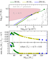 |
Fig. 14. Top panel: temperature and density profiles for example models approaching the instability, i.e., the first time ⟨Γ1⟩−4/3 = 0.01. The filled circles mark the central conditions at this stage. The green, yellow, and blue lines show examples of PPI+CC, PISN, and CC above the mass gap, respectively. All three examples are labeled according to their MHe, init. The red area marks the region of the EOS where pair-production results in an (local) instability. Bottom panel: values of the adiabatic index in the center when approaching the instability for the entire grid. The thin vertical lines mark the MCO of the examples models of the corresponding color in the top panel. |
The middle panel of Fig. 14 shows the local value of the adiabatic index in the center Γ1, c across our grid, also plotted when each model first reaches ⟨Γ1⟩−4/3 = 0.01. The bottom panel of Fig. 14 shows the innermost unstable mass coordinate Mu, i.e. the innermost location where Γ1 < 4/3. The colors in the middle and bottom panel have the same meaning as in Fig. 2. Overall, as MCO increases, the central value of the adiabatic index Γ1, c at the beginning of the instability decreases, and the location of the instability moves inward. However, this trend is not completely monotonic in the central part of the PPI+CC regime.
Two example models that ultimately result in a core collapse are shown in the top panel of Fig. 14. The green line corresponds to our MHe, init = 50 M⊙ example for PPI+CC, which shows more features compared to the other models, because the chemical stratification is more important in lower mass models. The central region of the 50 M⊙ model has a local value of the adiabatic index Γ1, c − 4/3 > 0.01 when ⟨Γ1⟩≃4/3, i.e., the center is stable when the averaged ⟨Γ1⟩ approaches instability. The deepest interior is too dense to become unstable: the contribution of radiation pressure to the total pressure decreases and the e± pairs fill the available continuum energy levels, raising the Fermi energy  and consequently the minimum energy photons need to produce a pair, preventing layers from undergoing the runaway instability (e.g., Zeldovich & Novikov 1999). This is true for all our PPI+CC models: in the bottom panel of Fig. 14, all the green points corresponding to PPI+CC have central values Γ1, c − 4/3 > 0.01 when ⟨Γ1⟩−4/3 = 0.01.
Since all our models are strongly radiation pressure dominated, they evolve with most of the mass along the Γ1 ≃ 4/3 locus on the (ρ, T)-plane, and when the instability starts, a nearly homologous contraction ensues. However, in the densest part of the core, neutrino cooling dominates over the energy release of the burning. Therefore, the net energy release starts off-center in our 50 M⊙ example, and because of the assumption of spherical symmetry, the energy release occupies a spherical mass shell. However, in nature the ignition might not happen simultaneously across the entire spherical shell, and this could potentially seed an asymmetric explosion. If asymmetries can build up rapidly during the pair-instability driven explosion (possibly aided by rotation), they could also lead to orbital “kicks” when PPI happens in a binary (Marchant et al. 2019).
The location of the unstable layer at the onset of the instability and of the location where the instability triggers net energy release both move inward toward the center as MHe, init and MCO increase. The least massive models to go PISN are characterized by having their center close to the instability, i.e., Γ1, c − 4/3 ≤ 0.01, when ⟨Γ1⟩−4/3 = 0.01 for the first time, as shown by the yellow filled circles in the bottom panel and the yellow solid line corresponding to MHe, init = 81 M⊙ in the top panel of Fig. 14. Our least massive PISN model has MHe, init = 80.75 M⊙ (corresponding to MCO = 54.89 M⊙) and a central value Γ1, c − 4/3 = 0.01 at this evolutionary stage. This model has Mu ≃ 0.05 M⊙ (shown as a dashed horizontal line in the bottom panel of Fig. 14), i.e. the unstable layer extends almost all the way to the center.
Models forming a BH above the PISN mass gap (cf. blue line in the top panel of Fig. 14 for a MHe, init = 250 M⊙ He core) are also unstable in their very center when ⟨Γ1⟩ reaches 4/3, but the ensuing thermonuclear explosion does not cause either pulses or full disruption. The different outcome is not caused by lack of energy released in the explosions, but rather by the inefficient use of that energy (Bond et al. 1984).
To summarize, the temperature, composition, and density profile of the star when it approaches the instability (i.e., ⟨Γ1⟩−4/3 = 0.01 for the first time) are indicative of its future evolution. In particular, the local value of the adiabatic index in the center Γ1, c at this point can be used to approximately distinguish PISN evolution with no BH remnant (if also Γ1, c − 4/3 ≤ 0.01) or PPI+CC evolution with a BH remnant (if instead the center is safely stable with Γ1, c − 4/3 > 0.01 when the star as a whole is becoming unstable). This provides a criterion to decide the final fate of a star without having to compute the hydrodynamical phase.
9.2. CSM structure and composition
We described in Sect. 6 the amount of mass ejected, its initial velocity, and the ejection timing resulting from our simulations. We typically keep the ejecta on our Lagrangian grid for several timesteps after ejection (until either the bound layers have recovered hydrostatic equilibrium or the onset of CC is reached). These ejected layers are moving significantly faster than the escape velocity and the sound speed, and our PPI+CC models exhibit an overall velocity gradient increasing outward so the ejecta do not cause any back-reaction on the inner layers that remain bound. Based on the initial mass, velocity, and time of the ejections, Sect. 6 illustrates the main features we expect in the CSM structure surrounding these stars with a toy model assuming propagation at constant velocity of the ejecta. This is an oversimplification, since the low density ejecta are likely to be optically thin and thus can lose energy radiatively. Moreover, as previously noted by Woosley (2017), the ejected shells can in many cases collide with each other, and this could also significantly change the CSM structure at the end. Multidimensional radiation hydrodynamics calculations using our results as input for the mass, chemical composition, and thermal state of the ejecta could be used to predict more robustly the CSM structure around PPI+CC models for comparison with observed transients, and to address the question of how many progenitors might reach the final CC embedded in a optically-thick layer of previously ejected material.
Another assumption in our calculations is that the presence of a H-rich envelope can be neglected to study the dynamics of PPI (Woosley 2017, 2019) and that, even if present, such a envelope would be removed early in the evolution by winds or binary interactions. Should a star retain some H-rich material until the onset of the first pulse, we can estimate if it would be detectable in the CSM surrounding these stars assuming that (i) the PPI-driven mass loss timing is unaffected by the presence of the H-rich envelope and (ii) the entire envelope is ejected in the first pulse (Woosley 2017).
To estimate the ejection velocities and radii of the H-rich material, we ran a H-rich 140 M⊙ model with initial He abundance Y = 0.27 and metallicity Z = 0.001 with the same setup as in our grids. In Appendix B, we compare this model to a He core of 55.25 M⊙ which produces a MCO ≃ 39.41 M⊙, similar in mass to the CO core produced by the H-rich 140 M⊙ star. The H-rich model reaches the onset of the PPI (⟨Γ1⟩−4/3 = 0.01) with Γ1, c − 4/3 = 0.05, so we expect it to follow the PPI+CC evolutionary path based on Sect. 9.1. This expectation is confirmed by our results presented in Appendix B. At the onset of the instability and with our assumed wind mass loss, this model has a total mass of Mtot = 83.2 M⊙, a He core of MHe ≃ 50 M⊙, and a CO core of MCO ≃ 39 M⊙. The remaining envelope has a mass of Menv ≡ Mtot − MHe ≃ 33 M⊙, however, the composition of this envelope is dominated by He, with a H mass fraction of X ≃ 0.14, since the winds have carved out material down to the initial location of the main sequence core of the star. At this stage, the envelope spans from the He core edge at RHe core = 0.58 R⊙ to R* = 3637 R⊙, so it is significantly extended.
If we assume propagation at constant velocity of this envelope, we can estimate the minimum and maximum radii (Rmin and Rmax, respectively) of this H-rich material at the time of the final CC and its average density (⟨ρ⟩) with
 (3)
(3)
where tCC − tpulse end ≃ 10 years based on the MHe and MCO of this model and Fig. 9. If we assume both escape velocities to be the stellar surface escape velocity, i.e.,  , then the CSM layer containing H would be at Rmin ≃ 1015.46 cm ≲ r ≲ Rmax ≃ 1015.51 cm and have an average density of ⟨ρ⟩≃2.2 × 10⁻¹² g cm−3.
Instead, if we assume,  is the velocity from the He core edge, while keeping the same vesc, out, then we obtain Rmax < Rmin (meaning there would necessarily be collisions internal to the ejecta that our simplistic toy model ignores). Nevertheless, the minimum radius at which we would expect CSM with H in it form the PPI mass ejection is Rmax ≃ 3.2 × 1016 cm and such layer would have an average density of ⟨ρ⟩≃3 × 10⁻¹⁸ g cm−3. The large difference between these two estimates is mostly due to the large radial extent of the envelope.
10. Conclusions
The broad theoretical understanding of the predicted pair-instability driven transients has been well established for several decades, however they remain somewhat elusive from an observational perspective. Recent developments in stellar evolution calculations allow for the exploration of synergies between gravitational waves and time-domain observations to better understand the formation process of the most massive stellar BHs.
We have computed a grid of naked He star models in the mass range 35 M⊙ ≤ MHe, init ≲ 250 M⊙ to investigate whether these would experience phases of global dynamical instability and pulsational mass loss due to the pair-production instability. We have computed grids at two different metallicities, Z = 0.001 and Z = 0.00198 = 14% Z⊙, although the main features we discuss are not significantly dependent on Z (except for the wind mass loss rate, see also Farmer et al. 2019). All our input files and numerical results are available online10.
Figure 15 summarizes our main results across the mass range considered. We find, in agreement with previous studies, that stars enter into the PPI regime progressively. The production of e± initially causes “oscillations” of the core temperature and nuclear luminosity at the lowest mass end. The least massive models experiencing an explosive thermonuclear ignition (MHe, init ≳ 37.5 M⊙) do not suffer significant global consequences (“weak pulses”). Increasing further the initial He core mass, the pulses become progressively stronger, causing at first large radial expansions (for initial 41 ≲ MHe, init ≲ 42 M⊙), and finally (for initial MHe, init ≳ 42 M⊙) also the ejection of matter. The values quoted here are for the initial He core mass of our models, which can be interpreted as the core mass at the end of the main sequence of the star. The mapping of these values to the final (preinstability) He core mass is mass loss and metallicity dependent (see also Farmer et al. 2019).
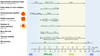 |
Fig. 15. Summary of the pair-instability driven behavior of models as a function of their initial He core mass (MHe, init) and maximum carbon-oxygen core mass (MCO). The approximate SN type in the top row speculates on what the resulting SN would appear like, if the final collapse produces an explosion. |
The different effects of a pulsational pair instability event on the star allow for (at least) three different physically-motivated definitions of a “pulse”, depending on which observable is considered (Sect. 5). The number of pulses and which He and CO core masses produce pulses might vary significantly depending on the observable of interest.
The first definition of pulse we consider (Sect. 5.1) is based on the core thermonuclear ignition, following the historical development of studies of pair-instability evolution. We find that in the lowest mass models the core ignition does not produce an observable electromagnetic signal or a significant impact on the final BH mass: the nuclear energy released in the burning is redistributed and stored in the star without affecting significantly the outermost layers. The most promising way to detect directly these core-ignition events is through the variations in the neutrino luminosity.
The second definition is based on the radial expansion of the models in response to the core ignition (Sect. 5.2): this definition shifts the lower edge of the pulsating regime upward in mass. For the most massive pulsating models (which also eject mass), the radial expansion itself might be hidden behind a pseudo-photosphere in the ejected layers. Because of the rarity of these stars in the local Universe, the most promising way to detect these radius variations may be through their enhancement of the rate of binary interactions (e.g., Marchant et al. 2019), although nearby stars that might undergo this evolution in the future exist (e.g., Bestenlehner et al. 2011; Crowther et al. 2016; Renzo et al. 2019).
The third definition is based on the ejection of mass (Sect. 5.3), which impacts both the circumstellar material around these stars and the final BH mass they produce. The ejected matter creates shells of ejecta surrounding the star. If the final collapse results in a successful (even if weak) explosion, the final SN ejecta can hit this PPI-produced CSM and convert kinetic energy into radiation.
In our grid, we find full disruption in a PISN for an initial He core mass of MHe, init ≃ 80 M⊙ corresponding to a final He core mass of MHe ≃ 60 M⊙ and MCO = 55 M⊙ after the wind mass loss. With our assumptions for the wind mass loss and metallicity, most PISN models would still retain He-rich material at their surface at the onset of the explosion. We propose a simplified criterion to distinguish full disruption in a PISN from pulsational behavior producing a final BH based on the adiabatic index at the center of the star Γ1, c ≲ 0.01 at the onset of the instability, defined as the first moment when the volumetric pressure-weighted average of the adiabatic index ⟨Γ1⟩−4/3 = 0.01 (Sect. 9.1). This threshold value allows for the approximately estimate the fate of a stellar model without the need to compute the hydrodynamical evolution.
The signature on the final BH masses is potentially detectable with a population of gravitational wave sources (Fishbach & Holz 2017; Talbot & Thrane 2018; Stevenson et al. 2019; Mangiagli et al. 2019). Only for MHe, init ≳ 42 M⊙ (MCO ≃ 30.75 M⊙) is the stellar core mass significantly reduced and the circumstellar material significantly affected, as shown in Fig. 15. The maximum BH mass below the PISN mass gap that we find is ∼45 M⊙ and it is formed by the collapse of an initially MHe, init ≃ 62 M⊙ (MCO ≃ 43.5 M⊙) He core that went through pulsational mass loss. More massive He cores also produce BHs, but because of the stronger mass loss due to winds and pair-instability driven pulses, the resulting BH masses are smaller.
Pair instability does not result in full disruption of the star for an initial He core mass of MHe, init ≃ 200 M⊙, which forms a BH of mass MBH = 125 M⊙ after wind mass loss. Above this He core mass, the photodisintegration of newly synthesized heavy elements during the thermonuclear explosion prevents the disruption of the entire star (e.g., Bond et al. 1984). The boundaries between PISN and BH formation we find are in very good agreement with previously published results.
We have characterized the CSM properties around the pulsating models resulting in mass ejections by assuming unperturbed constant velocity propagation of the ejecta. Under this simplifying assumption, we find that the CSM mass grows almost monotonically with the initial MHe, init from ∼10−6 M⊙ (for MHe, init ≃ 42 M⊙) to ∼20 M⊙ at the edge of the PISN range. For initial MHe, init ≳ 50 M⊙, the combined ejection of matter and mixing during a pulse propagation make He less abundant than C and O at the stellar surface at the onset of the final core-collapse. The stellar surface at the onset of core collapse might be obscured by the previously ejected layers.
The velocity of the ejecta is a few thousand km s−1, with the first mass-loss event often resulting in larger velocities. Nevertheless, with our assumptions, we find numerous self-collisions of the ejecta with previously ejected layers in agreement with the predictions of Woosley et al. (2007) and Woosley (2017). This velocity range is close to the width of narrow He lines detected in some SN Ibn.
The timing of pair-instability driven mass ejections also spans a large range of values, with a systematic trend of longer delays between pulses for the more massive models. This is because more massive models produce more energetic pulses that require a longer time (up to ∼104 years) for the star to recover its equilibrium.
With the velocity and timing of the ejecta produced by our models, we expect the PPI-produced circumstellar material to be at ∼1012 − 1016 cm away from the collapsing star at the end of its evolution. This range covers the distances inferred in observational candidates for pulsational pair instability evolution.
Gravitational wave detections of merging binary black holes are rapidly accumulating during the third LIGO/Virgo observing run, and currently available constraints on their mass will soon become statistically stringent. Together with the ongoing and upcoming large time-domain survey which will reveal a plethora of transient, including rare and exotic ones, this will provide direct constraints on pair-instability evolution of the most massive stars. Thus, in the future, gravitational and transient observations will soon shed light on the pair-instability evolution of the most massive stars and the BHs these produce.
The “first gap” is the apparent lack of compact objects with masses between the maximum neutron star mass, max{MNS}≃2 M⊙ and the least massive BH known min{MBH}≃5 M⊙, (e.g., Farr et al. 2011, but see also Wyrzykowski et al. 2016; Wyrzykowski & Mandel 2020).
The effect of rotation on the explosion dynamics has been investigated in Glatzel et al. (1985), Chatzopoulos et al. (2013).
cf. Eq. (2) in Paxton et al. (2011) and the MESA documentation for the definition of f and f0 .
Other events have since been reported by an independent analysis of the first two observing runs, see Zackay et al. (2019) and references therein.
In none of our models is such an upper limit in radius reached by the bound material.
Publicly available at https://doi.org/10.5281/zenodo.3406356
Since our models do not have a H-rich envelope, this is the total mass when the central He mass fraction reaches Xc(4He) < 10−5. We emphasize that this value is sensitive to the adopted wind mass loss rates.
Acknowledgments
We are grateful for the in depth reading of the referee and the suggested improvements to this manuscript. We acknowledge helpful discussions with M. Cantiello, D. Hendricks, E. Laplace, I. Mandel, B. Paxton, F. Timmes, L. van Son, and A. Vigna-Gómez. MR, SJ, and SdM acknowledge funding by the European Union’s Horizon 2020 research and innovation programme from the European Research Council (ERC) (Grant agreement No. 715063), and by the Netherlands Organisation for Scientific Research (NWO) as part of the Vidi research program BinWaves with project number 639.042.728. RF is supported by the Netherlands Organisation for Scientific Research (NWO) through a top module 2 grant with project number 614.001.501 (PI de Mink). EZ acknowledges support from the Swiss National Science Foundation Professorship grant (project number PP00P2 176868) and from the Federal Commission for Scholarships for Foreign Students for the Swiss Government Excellence Scholarship (ESKAS No. 2019.0091) for the academic year 2019-2020. Simulations were carried out on the Dutch national e-infrastructure (Cartesius, project number 16343) with the support of the SURF Cooperative.
References
- Abbott, B. P., Abbott, R., Abbott, T. D., et al. 2017, Phys. Rev. Lett., 118, 221101 [NASA ADS] [CrossRef] [PubMed] [Google Scholar]
- Abbott, B. P., Abbott, R., Abbott, T. D., et al. 2019, Phys. Rev. X, 9, 031040 [Google Scholar]
- Adams, S. M., Kochanek, C. S., Gerke, J. R., Stanek, K. Z., & Dai, X. 2017, MNRAS, 468, 4968 [NASA ADS] [CrossRef] [Google Scholar]
- Aoki, W., Tominaga, N., Beers, T. C., Honda, S., & Lee, Y. S. 2014, Science, 345, 912 [NASA ADS] [CrossRef] [PubMed] [Google Scholar]
- Arcavi, I., Hosseinzadeh, G., Howell, D. A., et al. 2017, Nature, 551, 64 [NASA ADS] [CrossRef] [Google Scholar]
- Arnett, W. D. 1969, Ap&SS, 5, 180 [NASA ADS] [CrossRef] [Google Scholar]
- Atri, P., Miller-Jones, J. C. A., Bahramian, A., et al. 2019, MNRAS, 489, 3116 [NASA ADS] [CrossRef] [Google Scholar]
- Barkat, Z., Rakavy, G., & Sack, N. 1967, Phys. Rev. Lett., 18, 379 [NASA ADS] [CrossRef] [Google Scholar]
- Barnes, J., Duffell, P. C., Liu, Y., et al. 2018, ApJ, 860, 38 [NASA ADS] [CrossRef] [Google Scholar]
- Belczynski, K., Heger, A., Gladysz, W., et al. 2016, A&A, 594, A97 [NASA ADS] [CrossRef] [EDP Sciences] [Google Scholar]
- Bellm, E., Graham, M. J., Mahabal, A. A., & Seaman, R. 2014, in The Third Hot-wiring the Transient Universe Workshop, ed. P. R. Wozniak, 27 [Google Scholar]
- Bestenlehner, J. M., Vink, J. S., Gräfener, G., et al. 2011, A&A, 530, L14 [NASA ADS] [CrossRef] [EDP Sciences] [Google Scholar]
- Bond, J. R., Arnett, W. D., & Carr, B. J. 1984, ApJ, 280, 825 [NASA ADS] [CrossRef] [Google Scholar]
- Brandt, W. N., Podsiadlowski, P., & Sigurdsson, S. 1995, MNRAS, 277, L35 [NASA ADS] [Google Scholar]
- Chan, C., Müller, B., Heger, A., Pakmor, R., & Springel, V. 2018, ApJ, 852, L19 [NASA ADS] [CrossRef] [Google Scholar]
- Chan, C., Mueller, B., & Heger, A. 2020, MNRAS, 495, 3751 [CrossRef] [Google Scholar]
- Chatzopoulos, E., & Wheeler, J. C. 2012a, ApJ, 748, 42 [NASA ADS] [CrossRef] [Google Scholar]
- Chatzopoulos, E., & Wheeler, J. C. 2012b, ApJ, 760, 154 [NASA ADS] [CrossRef] [Google Scholar]
- Chatzopoulos, E., Wheeler, J. C., & Couch, S. M. 2013, ApJ, 776, 129 [NASA ADS] [CrossRef] [Google Scholar]
- Chen, K. J., & Woosley, S. E. 2020, ApJ, 897, 152 [NASA ADS] [CrossRef] [Google Scholar]
- Chen, K.-J., Woosley, S., Heger, A., Almgren, A., & Whalen, D. J. 2014, ApJ, 792, 28 [CrossRef] [Google Scholar]
- Chevalier, R. A., & Irwin, C. M. 2012, ApJ, 747, L17 [NASA ADS] [CrossRef] [Google Scholar]
- Couch, S. M., Warren, M. L., & O’Connor, E. P. 2019, ApJ, 890, 127 [Google Scholar]
- Coughlin, E. R., Quataert, E., Fernández, R., & Kasen, D. 2018, MNRAS, 477, 1225 [CrossRef] [Google Scholar]
- Crowther, P. A., Caballero-Nieves, S. M., Bostroem, K. A., et al. 2016, MNRAS, 458, 624 [NASA ADS] [CrossRef] [Google Scholar]
- de Mink, S. E., Cantiello, M., Langer, N., et al. 2009, A&A, 497, 243 [NASA ADS] [CrossRef] [EDP Sciences] [Google Scholar]
- de Mink, S. E., Sana, H., Langer, N., Izzard, R. G., & Schneider, F. R. N. 2014, ApJ, 782, 7 [NASA ADS] [CrossRef] [Google Scholar]
- Dessart, L., Hillier, D. J., Li, C., & Woosley, S. 2012, MNRAS, 424, 2139 [NASA ADS] [CrossRef] [Google Scholar]
- Ertl, T., Janka, H.-T., Woosley, S. E., Sukhbold, T., & Ugliano, M. 2016, ApJ, 818, 124 [NASA ADS] [CrossRef] [Google Scholar]
- Farmer, R., Fields, C. E., Petermann, I., et al. 2016, ApJS, 227, 22 [NASA ADS] [CrossRef] [Google Scholar]
- Farmer, R., Renzo, M., de Mink, S. E., Marchant, P., & Justham, S. 2019, ApJ, 887, 53 [CrossRef] [Google Scholar]
- Farr, W. M., Sravan, N., Cantrell, A., et al. 2011, ApJ, 741, 103 [NASA ADS] [CrossRef] [Google Scholar]
- Fishbach, M., & Holz, D. E. 2017, ApJ, 851, L25 [NASA ADS] [CrossRef] [Google Scholar]
- Foley, R. J., Smith, N., Ganeshalingam, M., et al. 2007, ApJ, 657, L105 [NASA ADS] [CrossRef] [Google Scholar]
- Fowler, W. A., & Hoyle, F. 1964, ApJS, 9, 201 [Google Scholar]
- Fragos, T., Willems, B., Kalogera, V., et al. 2009, ApJ, 697, 1057 [NASA ADS] [CrossRef] [Google Scholar]
- Fraley, G. S. 1968, Ap&SS, 2, 96 [NASA ADS] [CrossRef] [Google Scholar]
- Fryer, C. L., Woosley, S. E., & Heger, A. 2001, ApJ, 550, 372 [NASA ADS] [CrossRef] [Google Scholar]
- Gal-Yam, A., Mazzali, P., Ofek, E. O., et al. 2009, Nature, 462, 624 [NASA ADS] [CrossRef] [PubMed] [Google Scholar]
- Georgy, C., Meynet, G., Ekström, S., et al. 2017, A&A, 599, L5 [NASA ADS] [CrossRef] [EDP Sciences] [Google Scholar]
- Gilkis, A., Soker, N., & Papish, O. 2016, ApJ, 826, 178 [NASA ADS] [CrossRef] [Google Scholar]
- Glatzel, W., Fricke, K. J., & El Eid, M. F. 1985, A&A, 149, 413 [NASA ADS] [Google Scholar]
- Gomez, S., Berger, E., Nicholl, M., et al. 2019, ApJ, 881, 87 [CrossRef] [Google Scholar]
- Hamann, W. R., & Koesterke, L. 1998, A&A, 335, 1003 [Google Scholar]
- Hamann, W.-R., Koesterke, L., & Wessolowski, U. 1995, A&A, 299, 151 [NASA ADS] [Google Scholar]
- Heger, A., Fryer, C. L., Woosley, S. E., Langer, N., & Hartmann, D. H. 2003, ApJ, 591, 288 [NASA ADS] [CrossRef] [Google Scholar]
- Heger, A., & Woosley, S. E. 2002, ApJ, 567, 532 [NASA ADS] [CrossRef] [Google Scholar]
- Hosseinzadeh, G., Arcavi, I., Valenti, S., et al. 2017, ApJ, 836, 158 [NASA ADS] [CrossRef] [Google Scholar]
- Janka, H.-T. 2013, MNRAS, 434, 1355 [Google Scholar]
- Janka, H.-T. 2017, ApJ, 837, 84 [NASA ADS] [CrossRef] [Google Scholar]
- Kasen, D., Woosley, S. E., & Heger, A. 2011, ApJ, 734, 102 [NASA ADS] [CrossRef] [Google Scholar]
- Kippenhahn, R., & Weigert, A. 1967, ZAp, 65, 251 [Google Scholar]
- Kippenhahn, R., Weigert, A., & Weiss, A. 2013, Stellar Structure and Evolution (Springer-Verlag) [Google Scholar]
- Kozyreva, A., Kromer, M., Noebauer, U. M., & Hirschi, R. 2018, MNRAS, 479, 3106 [NASA ADS] [CrossRef] [Google Scholar]
- Kuroda, T., Kotake, K., Takiwaki, T., & Thielemann, F.-K. 2018, MNRAS, 477, L80 [NASA ADS] [CrossRef] [Google Scholar]
- Langer, N., Norman, C. A., de Koter, A., et al. 2007, A&A, 475, L19 [NASA ADS] [CrossRef] [EDP Sciences] [Google Scholar]
- Leung, S.-C., Nomoto, K., & Blinnikov, S. 2019, ApJ, 887, 72 [NASA ADS] [CrossRef] [Google Scholar]
- Lovegrove, E., & Woosley, S. E. 2013, ApJ, 769, 109 [NASA ADS] [CrossRef] [Google Scholar]
- LSST Science Collaboration (Abell, P. A., et al.) 2009, ArXiv e-prints [arXiv:0912.0201] [Google Scholar]
- Lunnan, R., Chornock, R., Berger, E., et al. 2018, ApJ, 852, 81 [NASA ADS] [CrossRef] [Google Scholar]
- Maeder, A., & Meynet, G. 2000, ARA&A, 38, 143 [Google Scholar]
- Mandel, I., & de Mink, S. E. 2016, MNRAS, 458, 2634 [NASA ADS] [CrossRef] [Google Scholar]
- Mangiagli, A., Bonetti, M., Sesana, A., & Colpi, M. 2019, ApJ, 883, L27 [NASA ADS] [CrossRef] [Google Scholar]
- Marchant, P., Langer, N., Podsiadlowski, P., Tauris, T. M., & Moriya, T. J. 2016, A&A, 588, A50 [NASA ADS] [CrossRef] [EDP Sciences] [Google Scholar]
- Marchant, P., Renzo, M., Farmer, R., et al. 2019, ApJ, 882, 36 [Google Scholar]
- Moriya, T. J., & Langer, N. 2015, A&A, 573, A18 [NASA ADS] [CrossRef] [EDP Sciences] [Google Scholar]
- Mösta, P., Ott, C. D., Radice, D., et al. 2015, Nature, 528, 376 [NASA ADS] [CrossRef] [Google Scholar]
- Müller, B. 2019, MNRAS, 1527 [Google Scholar]
- Nadezhin, D. K. 1980, Ap&SS, 69, 115 [NASA ADS] [CrossRef] [Google Scholar]
- Nieuwenhuijzen, H., & de Jager, C. 1990, A&A, 231, 134 [NASA ADS] [Google Scholar]
- Nugis, T., & Lamers, H. J. G. L. M. 2000, A&A, 360, 227 [NASA ADS] [Google Scholar]
- O’Connor, E., & Ott, C. D. 2011, ApJ, 730, 70 [NASA ADS] [CrossRef] [Google Scholar]
- O’Shaughnessy, R., Gerosa, D., & Wysocki, D. 2017, Phys. Rev. Lett., 119, 011101 [NASA ADS] [CrossRef] [Google Scholar]
- Ott, C. D., Roberts, L. F., da Silva Schneider, A., et al. 2018, ApJ, 855, L3 [NASA ADS] [CrossRef] [Google Scholar]
- Pastorello, A., Smartt, S. J., Mattila, S., et al. 2007, Nature, 447, 829 [NASA ADS] [CrossRef] [PubMed] [Google Scholar]
- Pastorello, A., Mattila, S., Zampieri, L., et al. 2008, MNRAS, 389, 113 [NASA ADS] [CrossRef] [Google Scholar]
- Paxton, B., Bildsten, L., Dotter, A., et al. 2011, ApJS, 192, 3 [Google Scholar]
- Paxton, B., Cantiello, M., Arras, P., et al. 2013, ApJS, 208, 4 [NASA ADS] [CrossRef] [Google Scholar]
- Paxton, B., Marchant, P., Schwab, J., et al. 2015, ApJS, 220, 15 [Google Scholar]
- Paxton, B., Schwab, J., Bauer, E. B., et al. 2018, ApJS, 234, 34 [NASA ADS] [CrossRef] [EDP Sciences] [Google Scholar]
- Paxton, B., Smolec, R., Schwab, J., et al. 2019, ApJS, 243, 10 [NASA ADS] [CrossRef] [PubMed] [Google Scholar]
- Rakavy, G., & Shaviv, G. 1967, ApJ, 148, 803 [NASA ADS] [CrossRef] [Google Scholar]
- Regos, E., Vinko, J., & Ziegler, B. L. 2020, ApJ, 894, 94 [NASA ADS] [CrossRef] [Google Scholar]
- Renzo, M., Ott, C. D., Shore, S. N., & de Mink, S. E. 2017, A&A, 603, A118 [NASA ADS] [CrossRef] [EDP Sciences] [Google Scholar]
- Renzo, M., de Mink, S. E., Lennon, D. J., et al. 2019, MNRAS, 482, L102 [NASA ADS] [CrossRef] [Google Scholar]
- Renzo, M., Farmer, R. J., Justham, S., et al. 2020, MNRAS, 493, 4333 [CrossRef] [Google Scholar]
- Soker, N. 2019, Res. Astron. Astrophys., 19, 095 [CrossRef] [Google Scholar]
- Spera, M., & Mapelli, M. 2017, MNRAS, 470, 4739 [Google Scholar]
- Spera, M., Mapelli, M., Giacobbo, N., et al. 2019, MNRAS, 485, 889 [NASA ADS] [CrossRef] [Google Scholar]
- Stevenson, S., Sampson, M., Powell, J., et al. 2019, ApJ, 882, 121 [Google Scholar]
- Stothers, R. B. 1999, MNRAS, 305, 365 [NASA ADS] [CrossRef] [Google Scholar]
- Takahashi, K. 2018, ApJ, 863, 153 [Google Scholar]
- Talbot, C., & Thrane, E. 2018, ApJ, 856, 173 [NASA ADS] [CrossRef] [Google Scholar]
- Tolstov, A., Nomoto, K., Blinnikov, S., et al. 2017, ApJ, 835, 266 [NASA ADS] [CrossRef] [Google Scholar]
- Toro, E. F., Spruce, M., & Speares, W. 1994, Shock Waves, 4, 25 [NASA ADS] [CrossRef] [EDP Sciences] [Google Scholar]
- Tramper, F., Sana, H., & de Koter, A. 2016, ApJ, 833, 133 [NASA ADS] [CrossRef] [Google Scholar]
- Ugliano, M., Janka, H.-T., Marek, A., & Arcones, A. 2012, ApJ, 757, 69 [NASA ADS] [CrossRef] [Google Scholar]
- van den Heuvel, E. P. J., & Portegies Zwart, S. F. 2013, ApJ, 779, 114 [NASA ADS] [CrossRef] [EDP Sciences] [Google Scholar]
- Vigna-Gómez, A., Justham, S., Mandel, I., de Mink, S. E., & Podsiadlowski, P. 2019, ApJ, 876, L29 [CrossRef] [Google Scholar]
- Vink, J. S., & de Koter, A. 2005, A&A, 442, 587 [NASA ADS] [CrossRef] [EDP Sciences] [Google Scholar]
- Vink, J. S., de Koter, A., & Lamers, H. J. G. L. M. 2000, A&A, 362, 295 [Google Scholar]
- Vink, J. S., de Koter, A., & Lamers, H. J. G. L. M. 2001, A&A, 369, 574 [NASA ADS] [CrossRef] [EDP Sciences] [Google Scholar]
- Wang, S. Q., & Li, L. 2019, ApJ, submitted, [arXiv:1905.12623] [Google Scholar]
- Whalen, D. J., Even, W., Frey, L. H., et al. 2013, ApJ, 777, 110 [NASA ADS] [CrossRef] [Google Scholar]
- Wongwathanarat, A., Janka, H.-T., & Müller, E. 2013, A&A, 552, A126 [NASA ADS] [CrossRef] [EDP Sciences] [Google Scholar]
- Woosley, S. E. 2017, ApJ, 836, 244 [NASA ADS] [CrossRef] [Google Scholar]
- Woosley, S. E. 2018, ApJ, 863, 105 [NASA ADS] [CrossRef] [Google Scholar]
- Woosley, S. E. 2019, ApJ, 878, 49 [NASA ADS] [CrossRef] [Google Scholar]
- Woosley, S. E., Heger, A., & Weaver, T. A. 2002, Rev. Mod. Phys., 74, 1015 [NASA ADS] [CrossRef] [Google Scholar]
- Woosley, S. E., Blinnikov, S., & Heger, A. 2007, Nature, 450, 390 [NASA ADS] [CrossRef] [PubMed] [Google Scholar]
- Wyrzykowski, Ł., & Mandel, I. 2020, A&A, 636, A20 [NASA ADS] [CrossRef] [EDP Sciences] [Google Scholar]
- Wyrzykowski, Ł., Kostrzewa-Rutkowska, Z., Skowron, J., et al. 2016, MNRAS, 458, 3012 [NASA ADS] [CrossRef] [Google Scholar]
- Yoon, S.-C., Langer, N., & Norman, C. 2006, A&A, 460, 199 [NASA ADS] [CrossRef] [EDP Sciences] [Google Scholar]
- Yoon, S.-C., Dierks, A., & Langer, N. 2012, A&A, 542, A113 [NASA ADS] [CrossRef] [EDP Sciences] [Google Scholar]
- Yoon, S.-C., Dessart, L., & Clocchiatti, A. 2017, ApJ, 840, 10 [NASA ADS] [CrossRef] [Google Scholar]
- Yoshida, T., Umeda, H., Maeda, K., & Ishii, T. 2016, MNRAS, 457, 351 [NASA ADS] [CrossRef] [Google Scholar]
- Zackay, B., Venumadhav, T., Dai, L., Roulet, J., & Zaldarriaga, M. 2019, Phys. Rev. D, 100, 023007 [Google Scholar]
- Zeldovich, Y. B., & Novikov, I. D. 1999, Stars and Relativity, eds. K. S. Thorne, & W. D. Arnett, (Mineola, NY: Dover Publications) [Google Scholar]
Appendix A: Resolution study
We present here a study of the impact of the numerical resolution in Lagrangian mass coordinate and time on our results. We refer the interested readers to Marchant et al. (2019) for a study on the relaxation procedure and of the numerical resolution on the pulse mass loss, to Farmer et al. (2019) for a more comprehensive study of the impact of the numerical resolution and input physics variations on our PPI models, and Renzo et al. (2020) for a study of the impact of different treatments of time-dependent convection.
Figure A.1 shows the evolution in time of the amount of mass bound to the star (blue) and its core temperature (red) for two 50.0 M⊙ He core models computed with different resolutions. MESA offers many controls to fine-tune the resolution (see also the provided inlists and run_star_extras.f), here we vary only three parameters governing the overall variations of averaged quantities across adjacent mesh points and across timesteps. Our fiducial (higher) resolution uses mesh_delta_coeff = 0.8 (0.6) and split_merge_amr_nz_baseline = 8 000 (10 000) for the spatial resolution during the hydrostatic and hydrodynamical phases of evolution, respectively. The time discretization is controlled through varcontrol_target = 5d-5 (1d-5). The largest differences in the evolution are found after the onset of the PPI pulses, during the dynamical phase after log10{(tCC − t)/[yr]}≲ − 2. These result in a ΔM = 0.43 M⊙ difference in the mass remaining bound (and on the amount of mass ejected). We emphasize that even our fiducial value provides a resolution significantly higher than the MESA defaults, with a number of mesh points 1289 ≲ N ≲ 6311 and 87 900 timesteps from the onset of He core burning to the onset of core-collapse. For comparison, the higher-resolution model shown in Fig. A.1 has 1583 ≲ N ≲ 7908, however it is able to finish the evolution using a slightly smaller number of timesteps, 86165. This likely indicates that at the higher spatial resolution the most stringent condition on the timesteps is not varcontrol_target, and that the higher spatial resolution provides more numerical stability of the solution allowing for longer timesteps.
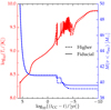 |
Fig. A.1. Mass (blue, right axis) and central temperature (red, left axis) evolution for our example 50 M⊙ example He core. The scale on the time axis emphasizes the short lived final phases. The differences in the final mass due to variations in the spatial and temporal mesh arise mostly from the dynamical phase of evolution and are limited to ΔM ≲ 0.5 M⊙. |
Appendix B: Comparison to H-rich model
A full characterization of PPI+CC evolution for stars with a H-rich envelope is beyond the scope of this study (we refer interested readers to Woosley 2017; Leung et al. 2019). Here, we present a brief comparison between a 140 M⊙ H-rich model (computed assuming and initial He abundance of Y = 0.27) and a MHe, init = 55.25 M⊙. Both these models produce MCO ≃ 40 M⊙.
Figure B.1 shows the evolution of the nuclear and neutrino luminosities (integrated throughout the entire star) and the central temperature of these two models. Even if there are some differences, the rough timing and amplitude of the oscillations of the core quantities are not significantly different during the pulses, i.e. during the last year of evolution. This is expected, since in general for all evolved massive stars the core evolution is not determined by the envelope. Instead, the evolution is driven by the neutrino losses from the core itself, rather than the photon luminosity at the surface (e.g., Fraley 1968).
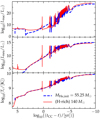 |
Fig. B.1. Comparison of the evolution of the nuclear luminosity (top) and neutrino luminosity (center) integrated throughout the star, and central temperature (bottom) for a H-rich initially 140 M⊙ star (red solid lines) to a MHe, init = 55.25 M⊙ core (blue dashed lines). Both models form a MCO ≃ 40 M⊙. |
Figure B.2 shows the evolution of the total, He and CO core masses for these two models. For the H-rich model, we define the He core as the outermost location where the H mass fraction is below 0.5 and the He mass fraction exceeds 0.1. If this yields zero, we set the He core mass equal to the total core mass. To avoid noise in the curve caused by mixing episodes at the core boundary at the end of the main sequence, we only show the He core mass once its value has stabilized. The H-rich model expells all its envelope at the first pulse about one year before CC. At this point the He core and the total mass become the same.
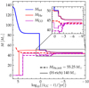 |
Fig. B.2. Comparison of the evolution of the total mass (blue), He core mass (red) and CO core mass (purple) for a 140 M⊙ H-rich model (solid) and a MHe, init = 55.25 M⊙ He-core (dashed). |
As shown in Table C.1, our 55.25 M⊙ model has three distinct mass-loss events. The comparison H-rich model also exhibits three mass-loss pulses. However, the timing in between the events is slightly different in the two models. This is partly due to the extreme sensitivity to the core masses (or, more precisely, the entropy profile) at the onset of the pulses. As well as the presence of the H-rich envelope, especially if extended, which increases the dynamical timescale and the delay between the core thermonuclear ignition and shock breakout and thus the mass ejection.
These two models, characterized by similar MCO (defined in Sect. 2 as the maximum throughout the evolution of the CO core mass) yield similar BH masses of ≃43.5 M⊙ for the He core and ≃45 M⊙ for the H-rich model. The difference between the BH mass values found here are smaller than those introduced by other physical and numerical uncertainties (Farmer et al. 2019).
Appendix C: Mass loss per pulse
Table C.1 provides data for each individual mass ejection event in our grid of models. We list the total mass at the beginning of the pulse  , the amount of mass lost ΔMpulse, the delay time between core-collapse and the end of the pulse, and the pulse duration Δtpulse, respectively (as defined in Sect. 5.3), and the center-of-mass velocity of the ejected layer ⟨v⟩. This table is also available at https://doi.org/10.5281/zenodo.3406356.
Number of pulses (pulse), prepulse total mass  , amount of mass lost in the pulse ΔMpulse, delay time between the pulse end tend and the final core-collapse and its duration Δtpulse (so that tpulse end = tpulse start + Δtpulse, cf. Fig. 9) according to the definition of Sect. 5.3, and the velocity of the center of mass of the ejected layers ⟨v⟩ for each PPI+CC model.
All Tables
He core mass at the beginning of our simulations (MHe, init) and at He depletion (MHe, depl), carbon-oxygen core mass (MCO), iron core mass (MFe), mass location M4 where the specific entropy is lower than 4kBNA, and mass gradient μ4 ≡ dM/dr|s = 4kBNA for a representative subset of our models eventually forming a BH at Z = 0.001.
Number of pulses (pulse), prepulse total mass , amount of mass lost in the pulse ΔMpulse, delay time between the pulse end tend and the final core-collapse and its duration Δtpulse (so that tpulse end = tpulse start + Δtpulse, cf. Fig. 9) according to the definition of Sect. 5.3, and the velocity of the center of mass of the ejected layers ⟨v⟩ for each PPI+CC model.
All Figures
|
Fig. 1. Evolution of a massive He core undergoing (pulsational) pair instability evolution. Three final outcomes are possible: full disruption without a compact remnant (4a.), formation of a BH because of the photodisintegration instability (4c.), or episodic mass loss (4b.) and final stabilization of the core, followed by a regular core-collapse event. |
| In the text | |
|
Fig. 2. Final BH masses as a function of the initial He core mass. The scale in the horizontal direction is logarithmic. The colors in the background indicate the approximate range for each evolutionary path, see also Sect. 3. Right panel: masses inferred from the first ten binary BH mergers detected by LIGO/Virgo, with a red shade to emphasize the overlap between PPI and CC, and green and blue hatches to indicate the fate of the progenitor in different BH mass ranges. |
| In the text | |
|
Fig. 3. Last year of evolution of the central temperature (blue, bottom panel), nuclear (red) and neutrino (orange) luminosity (top panel) for a 50 M⊙ He core. The inset in the bottom panel shows the readjustment of the core to hydrostatic equilibrium after the first pulse, which we resolve even if this behavior is likely to be influenced by the imposed spherical geometry. |
| In the text | |
|
Fig. 4. Radial evolution of a Minit = 50 M⊙ He core through PPI pulses. The radius of the bound material (red, plotted only during dynamical phases) oscillates because of the PPI. The photospheric radius (orange) reaches 104 R⊙ (dashed line) during the dynamical phase of evolution, i.e., the location at optical depth 2/3 is in the material already ejected. |
| In the text | |
|
Fig. 5. Space-time diagram for propagation of the PPI ejecta of a 50 M⊙ He core. The color indicates the density, assuming radial expansion at constant velocity. The top panel indicates the cumulative amout of ejected at velocities larger than the escape velocity through pulses only (i.e., excluding the wind mass loss). The cyan curve shows the radius of the material instantaneously bound (cf. the red curve in Fig. 4). |
| In the text | |
|
Fig. 6. Number of mass-ejection events caused by pair instability as a function of CO core mass. The color shading indicates the approximate range for each behavior: core collapse without experiencing PPI-driven mass loss (CC, blue), PPI-driven mass loss (PPI+CC, green), or full disruption in a PISN (yellow), which we define as one mass loss event. The noisiness is caused by the occurrence of mass loss event right at the time of the final core collapse. |
| In the text | |
|
Fig. 7. Velocity profile at the onset of core-collapse for a 50 M⊙ He core, which undergoes a PPI mass-loss event while collapsing. The dashed red line shows the escape velocity profile, the thick blue line indicates the profile of the bound material, while the thinner line represents material still on the Lagrangian mass grid, but already beyond the escape velocity. The gray area indicates the model dependent amount of mass lost to stellar winds. |
| In the text | |
|
Fig. 8. PPI-driven mass loss as a function of the CO core mass. Top panel: total mass ejected in pulses, bottom panel: mass lost in individual pulses. The amount of mass lost does not have a monotonic behavior with pulse number, and spans a wide range of values. The first pulse is shown as a blue dot, and the second and third, if they occur, are shown as a purple plus and red cross, respectively. Thin vertical lines connect multiple pulses for the same MCO. |
| In the text | |
|
Fig. 9. Delay time between the final core-collapse and the end of each mass loss event in a PPI pulse. Typical delays are on the order of few months, but they increase steeply with the initial He core mass of the PPI progenitor, which produce fewer but more energetic pulses, up to 104 years. The top inset magnifies the range of half a year delays on a days scale. The first pulse is shown as a blue dot, and the second and third, if occurring, are shown as a purple plus and red cross, respectively, with a thin blue line connecting the pulses of the same model. |
| In the text | |
|
Fig. 10. Center-of-mass velocity of the layers ejected at each pulse. The first pulse (blue filled circles) produces typically higher ejection velocities, and the ejecta move at ∼ few thousand km s−1 which suggests a connection with (some subclasses) of SN Ibn. |
| In the text | |
|
Fig. 11. 56Ni mass present in the deep interior of the star at the onset of CC or PISN. The color background is the same as Fig. 6 and indicates the approximate evolution (CC for blue, PPI+CC for green, and PISN for yellow). We computed these models using a 22-isotope nuclear reaction network. |
| In the text | |
|
Fig. 12. CC and PPI+CC models on the Ertl criterion plane for “explodability”. The red area indicates the uncertain boundary region between successful explosions and neutron star formation (white) and collapse with BH formation (gray). The dotted rectangle in the bottom left indicates the range originally showed in Ertl et al. (2016), most of our models require extrapolating outside this range. Blue dots correspond to CC models, while green dots show PPI+CC models. |
| In the text | |
|
Fig. 13. Surface composition at the onset of core-collapse for the PPI+CC and CC models. 4He, 12C, 16O are shown as red filled circles, cyan triangles, and blue crosses, respectively. The dot-dashed horizontal lines of the same color mark the initial mass fraction for these elements for our Z = 0.001 model grid. The colored background indicates the approximate evolution of the star (cf. Fig. 2 and Sect. 3). |
| In the text | |
|
Fig. 14. Top panel: temperature and density profiles for example models approaching the instability, i.e., the first time ⟨Γ1⟩−4/3 = 0.01. The filled circles mark the central conditions at this stage. The green, yellow, and blue lines show examples of PPI+CC, PISN, and CC above the mass gap, respectively. All three examples are labeled according to their MHe, init. The red area marks the region of the EOS where pair-production results in an (local) instability. Bottom panel: values of the adiabatic index in the center when approaching the instability for the entire grid. The thin vertical lines mark the MCO of the examples models of the corresponding color in the top panel. |
| In the text | |
|
Fig. 15. Summary of the pair-instability driven behavior of models as a function of their initial He core mass (MHe, init) and maximum carbon-oxygen core mass (MCO). The approximate SN type in the top row speculates on what the resulting SN would appear like, if the final collapse produces an explosion. |
| In the text | |
|
Fig. A.1. Mass (blue, right axis) and central temperature (red, left axis) evolution for our example 50 M⊙ example He core. The scale on the time axis emphasizes the short lived final phases. The differences in the final mass due to variations in the spatial and temporal mesh arise mostly from the dynamical phase of evolution and are limited to ΔM ≲ 0.5 M⊙. |
| In the text | |
|
Fig. B.1. Comparison of the evolution of the nuclear luminosity (top) and neutrino luminosity (center) integrated throughout the star, and central temperature (bottom) for a H-rich initially 140 M⊙ star (red solid lines) to a MHe, init = 55.25 M⊙ core (blue dashed lines). Both models form a MCO ≃ 40 M⊙. |
| In the text | |
|
Fig. B.2. Comparison of the evolution of the total mass (blue), He core mass (red) and CO core mass (purple) for a 140 M⊙ H-rich model (solid) and a MHe, init = 55.25 M⊙ He-core (dashed). |
| In the text | |
Current usage metrics show cumulative count of Article Views (full-text article views including HTML views, PDF and ePub downloads, according to the available data) and Abstracts Views on Vision4Press platform.
Data correspond to usage on the plateform after 2015. The current usage metrics is available 48-96 hours after online publication and is updated daily on week days.
Initial download of the metrics may take a while.