| Issue |
A&A
Volume 696, April 2025
|
|
|---|---|---|
| Article Number | A103 | |
| Number of page(s) | 26 | |
| Section | Stellar structure and evolution | |
| DOI | https://doi.org/10.1051/0004-6361/202453426 | |
| Published online | 18 April 2025 | |
Mass-transferring binary stars as progenitors of interacting hydrogen-free supernovae
1
Argelander Institut für Astronomie, Auf dem Hügel 71, DE-53121 Bonn, Germany
2
Max-Planck-Institut für Radioastronomie, Auf dem Hügel 69, DE-53121 Bonn, Germany
3
Institut d’Astrophysique de Paris, CNRS-Sorbonne Université, 98 bis boulevard Arago, F-75014 Paris, France
⋆ Corresponding author; This email address is being protected from spambots. You need JavaScript enabled to view it.
Received:
13
December
2024
Accepted:
12
February
2025
Abstract
Context. Stripped-envelope supernovae (SNe) are hydrogen-poor transients produced at the end of the life of massive stars that have previously lost most or all of their hydrogen-rich envelope. The progenitors of most stripped-envelope SNe are thought to be donor stars in mass-transferring binary systems that were stripped of their hydrogen-rich envelopes some 106 yr before core collapse. A subset of the stripped-envelope SNe exhibit spectral and photometric features indicative of early, intense interactions between their ejecta and nearby circumstellar material (CSM) occurring within days or weeks of the explosion.
Aims. We examine whether Roche lobe overflow during or shortly before core collapse in massive binary systems can produce the CSM inferred from the observations of interacting H-poor SNe.
Methods. We selected 44 models from a comprehensive grid of detailed binary evolution models that are representative of the subset in which the mass donors are hydrogen-free and explode while transferring mass to a main-sequence companion. We characterized the properties of the pre-SN stellar models and of the material surrounding the binary at the time of the SN.
Results. We find that in these models, mass transfer starts less than ∼20 kyr before and often continues until the core collapse of the donor star. Up to 0.8 M⊙ of hydrogen-free material are removed from the donor star during this phase, and a large fraction may be lost from the binary system and produce He-rich circumbinary material. We explored plausible assumptions for its spatial distribution at the time of explosion. When assuming that the CSM accumulates in a circumbinary disk, we found qualitative agreement with the SN and CSM properties inferred from the observed Type Ibn SNe and to a lesser extent with constraints from Type Icn SNe. Considering the birth probabilities of our mass transferring stripped envelope SN progenitor models, we find that they may produce up to ∼10% of all stripped-envelope SNe.
Conclusions. The generic binary channel proposed in this work can qualitatively account for the observed key properties and the observed rate of interacting H-poor SNe. Models for the evolution of the circumbinary material and for the spectral evolution of exploding progenitors from this channel are needed to further test its significance.
Key words: binaries: general / circumstellar matter / stars: evolution / stars: massive / stars: mass-loss / supernovae: general
© The Authors
 Open Access article, published by EDP Sciences, under the terms of the Creative Commons Attribution License (https://creativecommons.org/licenses/by/4.0), which permits unrestricted use, distribution, and reproduction in any medium, provided the original work is properly cited.
This article is published in open access under the Subscribe to Open model. This email address is being protected from spambots. You need JavaScript enabled to view it. to support open access publication.
1. Introduction
Many massive stars end their lives as supernovae (SNe), bright transients that are observable even in distant galaxies. Past surveys (PTF, Law et al. 2009, and iPTF, Kulkarni 2013) and especially ongoing ones (e.g., ATLAS, Tonry et al. 2018; ASAS-SN, Kochanek et al. 2017; ZTF, Bellm et al. 2019) have dramatically increased the number of observed SNe over the past few decades, which has led to the discovery of new, particular SN types. This is expected to continue in the coming years and decades, particularly thanks to the beginning of new surveys such as the Legacy Survey of Space and Time (LSST; Ivezić et al. 2019).
These surveys are providing growing evidence that the light of as much as ∼10% of all core-collapse SNe (CC-SNe) is affected, sometimes even dominated, by the interaction of the SN ejecta with the circumstellar material (CSM) surrounding the exploding star (e.g., Perley et al. 2020). The relatively slow-moving CSM can produce narrow-line features in the SN spectrum, which prompts the classification of such transients as Type IIn (with narrow H-emission lines), Type Ibn (He), Type Icn (C/O), and even Type Ien (S/Si, Schulze et al. 2024) SNe. In some instances, the interaction power is so strong as to result in superluminous SNe (SLSNe; Chatzopoulos et al. 2012) and can also explain more exotic events such as some fast blue optical transients (FBOTs; e.g., AT-2018cow, Margutti et al. 2019; Pellegrino et al. 2022a; Ho et al. 2023). The observed presence of the CSM thus offers a valuable diagnostic for probing the late stages of stellar evolution.
Recent studies have investigated the characteristics of the CSM in interacting H-poor SNe through explosion modeling (e.g., Dessart et al. 2022; Takei et al. 2024) or by analyzing the light curves of observed events (e.g., Chatzopoulos et al. 2012, 2013). For Type Ibn and Icn SNe, not all events of the same class are associated with the same progenitor and CSM structure (e.g., Turatto & Pastorello 2014; Pellegrino et al. 2022b). Some, for example the Type Ibn SN 2019uo (Gangopadhyay et al. 2020) and the Type Icn SN 2022ann (Davis et al. 2023) are highly energetic explosions associated with massive Wolf–Rayet stars. Others, such as ultra-stripped (US) Type Ibn SN 2019dge (Yao et al. 2020), are much less energetic and likely originate from low-mass progenitors. These SNe prompt questions about the progenitors and the CSM required to explain the observations, as canonical single-star models struggle to reproduce the inferred CSM for these SNe.
Some works suggest that single stars can undergo strong phases of mass loss due to mechanisms such as thermonuclear flashes in the core (Woosley et al. 1980; Woosley & Heger 2015), wave-driven envelope excitations (Quataert & Shiode 2012; Wu & Fuller 2021), and eruptions associated to Luminous blue variables (LBVs; Smith & Arnett 2014). If triggered shortly before core collapse, these mechanisms not only produce the CSM but also explain the observed pre-SN outbursts associated with some interacting SNe.
Most massive stars are born as members of close binary systems (Sana et al. 2012), and many undergo mass transfer to their companion star through Roche lobe overflow (RLOF) during their evolution (Podsiadlowski et al. 1992). In most interacting binaries, this happens as a consequence of the post main-sequence (MS) expansion of the donor star, which occurs long before an SN explosion in the binary. However, some donor stars expand strongly after core helium exhaustion, which can trigger a late RLOF that continues until the mass donor's core collapses. For non-conservative mass transfer, this situation can lead to a dense CSM surrounding the binary system at the time of the SN explosion. This is found in binary evolution models containing H-rich (Matsuoka & Sawada 2024; Ercolino et al. 2024) or H-poor donor stars (Wu & Fuller 2022a, referred to hereafter as WF22). This binary channel enables stars of the same initial mass to follow various evolutionary paths, depending on their initial orbital configuration, which may relate to the variety of Type II SNe progenitors (e.g., in wide binaries: Ouchi & Maeda 2017; Matsuoka & Sawada 2024; Ercolino et al. 2024; Dessart et al. 2024) as well as Type IIb (Claeys et al. 2011; Sravan et al. 2019; Yoon et al. 2017) and Type Ibc SNe (Yoon et al. 2010; Dessart et al. 2011).
In stripped-envelope SNe, the exploding star is a naked He-star (HeS). It has been established that low-mass HeS (≲3.5 M⊙) expand strongly after core-helium burning (e.g., Paczyński 1971; Habets 1986; Woosley et al. 1995; Wellstein & Langer 1999; Yoon et al. 2010; Kleiser et al. 2018; Woosley 2019; Laplace et al. 2020; WF22). In binaries, this expansion can trigger mass transfer. If some of the transferred mass escapes the system, it could form the CSM near the binary, which may interact with the ejecta during the first SN explosion that occurs in the binary.
In this study, we investigate how interacting Type Ibc SNe can arise in binaries undergoing multiple phases of stable mass transfer. Unlike many studies that have focused on binaries with compact object companions, such as a black hole (BH; e.g., Jiang et al. 2023) or a neutron star (NS; e.g., Tauris et al. 2013, 2015; Jiang et al. 2021, 2023; Guo et al. 2024; WF22), this work examines the more abundant systems where the exploding star is the initially more massive star in the binary orbiting an MS companion. Although such binaries have been modeled before (e.g., Habets 1986; Laplace et al. 2020; WF22), we use a comprehensive approach here with the aim of covering the diversity of pre-SN CSM structures and exploring the frequency with which they occur in the universe.
The paper is structured as follows. We begin by detailing the physics of the stellar evolutionary models (Sect. 2) and the parameter space for pre-SN mass transfer (Sect. 3). We then analyze binary evolution models and their pre-SN properties (Sect. 4), which is followed by analysis of the impact of the CSM on the SN (Sect. 5) before a comparison between the model predictions with observed H-poor interacting SNe (Sect. 6). Finally, we discuss key physical processes and uncertainties that affect our results (Sect. 7) before summarizing the results (Sect. 8).
2. Method and assumptions
In this work we study binary models that develop into HeS+MS systems undergoing mass transfer shortly before CC (which we refer to as Case BC RLOF; see Sect. 3.2). These systems are potential progenitors of interacting H-poor SNe, assuming that some of the transferred mass escapes to form the CSM.
Three series of stellar evolutionary models run with MESA (r10398, Paxton et al. 2011, 2013, 2015, 2018, 2019) are used. The first is a comprehensive large-scale grid of previously calculated detailed binary evolutionary models (Jin et al., in prep.) which, due to the numerical settings used, do not produce many mass-transferring HeS+MS binaries (see Sect. 3). To expand the coverage of systems undergoing Case BC RLOF, we produce two other sets of models. The first is a set of detailed single HeS models, used to diagnose models in the binary grid where the stripped primary (i.e., the initially more massive star) is expected to expand and trigger Case BC RLOF. By comparing the binary grid with the single HeS models, we select and run a representative set of models in the binary grid up to CC, using improved physics and numerical settings to better tackle their evolution. Throughout this work, we refer to the HeS primary in a binary system as a binary-stripped HeS, in contrast to a single HeS model.
The three sets of models share key settings as described in Ercolino et al. (2024) and Jin et al. (2024), including the initial metallicity (Z=Z⊙, with Z⊙ = 0.154 from Asplund et al. 2021), and wind mass-loss prescription. In the following, we present the differences in the physics assumptions between the sets.
2.1. Initialization and rotation
In both the binary grid and our binary models, each star is initialized at the zero-age main sequence (ZAMS) with an initial rotation set to 20% of its breakup velocity (Dufton et al. 2013).
The single HeS models are initialized following Aguilera-Dena et al. (2022, 2023), where an MS star is evolved with artificial full mixing and no winds until core H depletion. Afterward, artificial mixing is disabled and the winds are introduced, allowing the model to evolve as a HeS. Rotation is neglected in single HeS models as, in the binary grid, the binary-stripped HeS models rotate very slowly during core He burning.
2.2. Nuclear network and termination
The binary grid adopts the stern nuclear network (Heger et al. 2000; Jin et al. 2024), and the models are terminated after the end of core C-burning, (Jin et al., in prep.; however, some models are also terminated beforehand; see Sect. 2.4).
We adopt the approx21 network in the single and binary-stripped HeS models, as it includes the bare minimum number of isotopes to evolve the models until CC. As our parameter space focuses on low-mass cores (see Sect. 3), the nuclear network adopted here is suboptimal (see Farmer et al. 2016). The next smallest viable nuclear network in MESA, which contains 75 isotopes, increases the computation time, hindering the feasibility of running a grid of models.
2.3. Overshooting and non-adiabatic convection
Overshooting is included in the convective H-burning core based on the initial mass, following Hastings et al. (2021). After core H-burning, overshooting is not included in any of the convective boundaries until the end of core C burning. After core C burning, when the models in the binary grid are terminated, our single and binary-stripped HeS models introduce small-scale over and undershooting across all convective boundaries, extending only 0.008HP from the boundary (with HP being the local pressure scale height at the convective boundary). This reduces computation difficulties, especially as successive core burning phases ignite off-center (see the example model in Sect. 4.1), causing convergence issues. Given the number of convective regions that develop as heavier elements are burnt, the adoption of convective over and undershooting may yield considerable differences in the final core structure.
Lastly, the binary grid adopts MLT++ (Paxton et al. 2015) to handle convectively unstable regions with inefficient energy transport (i.e., subsurface convective regions) by artificially reducing the local superadiabaticity. This can lead to smaller radii in models with convective layers near the surface, as well as density inversions. We therefore employ the standard MLT in both our single- and binary-stripped HeS models, rather than MLT++.
2.4. Roche lobe overflow
The binary grid of models adopts different mass transfer schemes depending on the primary star's evolutionary phase. If the primary is still an MS star, the mass transfer scheme is the “contact” scheme (Marchant et al. 2016). After the MS, the mass transfer scheme adopted is that of Kolb & Ritter (1990) to handle RLOF from a convective envelope.
Since we run binary models that begin RLOF after the MS (see Sect. 3), we adopt the scheme from Kolb & Ritter (1990), where we also consider the radiation pressure of the donor star in the mass-transfer calculation, as done in WF22. Our treatment is the same as that in Ercolino et al. (2024). We assume that the transferred mass also carries angular momentum and that accretion is halted when the accretor reaches critical rotation (Petrovic et al. 2005). In the models from the binary grid, this typically results in a small amount of mass being accreted, around ≲0.3 M⊙ during Case B RLOF. The mass that fails to be accreted is assumed to be lost from the binary system, carrying away the specific angular momentum of the accreting star. We assume that Case BC RLOF is completely inefficient (see Sect. 4.1).
In the binary grid, a model is terminated when unstable mass transfer and therefore common envelope (CE) evolution ensue. Unstable RLOF is assumed to occur if the model exhibits inverse mass transfer, RLOF at ZAMS, Darwin instability (Darwin 1879), or if it becomes an overcontact binary outflowing material from the L2 point. An additional stopping condition in the binary grid occurs when a model reaches a mass transfer rate of 10−1 M⊙ yr−1. We do not apply this condition in our binary models. We additionally consider mass transfer to turn unstable when the donor star reaches the volume-equivalent radius associated to its outer Lagrangian point (∼1.3RRL, 1, Marchant et al. 2021). This can lead to outer Lagrangian-point outflows (OLOF, Pavlovskii & Ivanova 2015; Ercolino et al. 2024). These conditions provide a broad parameter space to investigate models (but see Sect. 7.2.2 for a discussion using different assumptions).
3. Parameter space
The key ingredient for an interacting H-poor SN is the presence of a dense, H-poor CSM. Assuming that the CSM forms from the material not accreted by the companion star during RLOF shortly before CC, we search for H-poor donors that will undergo Case BC RLOF.
Since binary grid underestimates the parameter space for models undergoing Case BC RLOF (see Sect. 3.2), we aim to identify the systems that are expected to do so. We first investigate the radial expansion of single HeS models in their later evolutionary stages (Sect. 3.1). We then compare the single HeS models with the binary-stripped HeS models in the binary grid at the end of core He burning to assess which models are expected to undergo RLOF before CC (Sect. 3.2). This enables us to select the initial parameters of the models to recompute (Sect. 3.3).
3.1. Single HeS models
We computed single HeS models with initial masses between 2.99 and 5.31 M⊙ and focused on their radius evolution (see Table 1 and Fig. 1). During core He burning, these stars have radii below ∼1 R⊙. Stellar winds reduce their mass over time, resulting in a decrease of the convective He-burning core mass, which affects the final CO-core mass. We label the models by their mass at core He-depletion (MHe−dep), prefixed with “He”. For example, model He2.49 is the lowest-mass the model, with an initial mass Mi = 2.99 M⊙ and MHe−dep = 2.49 M⊙.
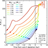 |
Fig. 1. Evolution of the radius of single HeS models as a function of time during and after core carbon burning, with t = 0 set at core carbon depletion. The square markers indicate core carbon ignition, circles indicate the time when the first carbon shell develops, and stars mark the end of the calculation. For the lowest mass model, no endpoint is shown (see Sect. 3.1). |
Properties of the single HeS models.
After core He-burning, shell He-burning drives the expansion of the He-rich envelope, which is more significant for lower mass models (see Fig. 1). The expansion continues during C-burning. In the lowest mass models, the expansion temporarily stalls (models He2.49, and He2.61), due to the more significant decrease of the power of the He-burning shell. The stellar expansion continues beyond core-C exhaustion. In the ∼2−3 kyr that follow the ignition of the first C-burning shell, the radius grows significantly, with the lowest mass models reaching ∼200 R⊙. More massive models (with MHe−dep>3.59 M⊙) explode before they can expand significantly. Following C-shell burning, the He-burning shell becomes convective for all models. In the least massive models, which developed the largest radii (i.e., models from He2.49 to He2.99), the outer envelope also turns convective.
After Ne and O ignite in the core, the envelope contracts significantly in smaller-mass models (see Fig. 1) but remains largely unaffected in higher-mass ones. Models He2.86 and He2.99 exhibit ingestion of He inside the CO core shortly before core-Si ignition, causing the envelope to expand. In the final stages before the end of the run, model He2.86 also exhibits a numerical oscillation of the envelope. In models He2.61 and He2.49, the surface and the He-burning convective regions merge, leading to significant radius expansion.
The key results of the simulations are shown in Table 1. All models, except the least massive, are expected to end their evolution as CC-SNe, even though many terminated shortly before CC. In particular, the models’ central density and temperature increase toward the end of the run, resembling the CC progenitors in Tauris et al. (2015). The lowest-mass model in the set (He2.49) evolves with an almost constant central temperature (below that achieved during core C burning) and increasing densities, resembling the electron-capture (EC) SN progenitor in Tauris et al. (2015). HeS models with similar masses to that of model He2.49 are expected to explode as EC-SNe, while those at lower masses will turn into a WD.
These models enable mapping of the radius's evolution as a function of mass of the HeS. We built a mass-radius diagram (see Fig. 2) showing how long before CC a single HeS of mass MHe−dep reaches a radius R.
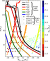 |
Fig. 2. Mass-radius diagram for single HeS models (showing the stellar radius, lines) and binary-stripped HeS models (showing the Roche lobe radius, symbols) as a function of the mass at core He-depletion MHe−dep. For single HeS models, the radius at a time t before the end of the run ( |

3.2. Comparing HeS models to the binary grid
Using the mass-radius map from single HeS models (Sect. 3.1), we identify the binary-stripped HeS models in the binary grid that are expected to undergo Case BC RLOF. This is done by comparing their Roche lobe radius (RRL, 1) with the expected radius evolution of a single HeS model with the same MHe−dep.
In the models in the binary grid where Case B is the first mass-transfer phase, the donor does not lose a fixed amount of mass or the entire H-rich envelope, as often assumed in rapid-binary evolution codes (e.g., ComBinE; Kruckow et al. 2018). Rather, the amount of mass-loss depends on the initial mass ratio (qi) and orbital period (Pi), leading to varying degrees of stripping for primaries of same initial mass (M1, i). Moreover, during core He burning, core growth depends on the mass of the leftover H-rich envelope (e.g., Ercolino et al. 2024). If the H-envelope mass is ≲1 M⊙, the long timescales for core-He burning allow stellar winds to shed it away entirely (though wind mass-loss rates are uncertain; see Sect. 7.1). These effects lead to the differences of up to 1 M⊙ in MHe−dep in stars of the same M1, i found in binaries (see Fig. 3).
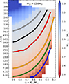 |
Fig. 3. Plot of the log Pi−qi diagram for the binary grid of models from Jin et al. (in prep.), with M1, i = 12.6 M⊙. Each pixel represents one detailed binary evolution model. The color coding represents the mass of the primary star at core helium depletion. The solid lines cover the models where the radius of a single HeS of the same mass (see Fig. 2) matches their Roche lobe radius at core He depletion. White pixels are models that terminated before core-carbon ignition (see Sect. 2.4). The dotted patches correspond to the models which exhibited Case BC RLOF in the binary grid. The star marker in the top-left corner corresponds to the lowest-period model shown in Ercolino et al. (2024). |
All Case B models in the binary grid exhibit RRL, 1≳5 R⊙ during core He burning, which is larger than the maximum radius expected from single HeS models in that phase (see Sect. 3.1). This implies that RLOF can only occur after core He depletion. Following core He depletion, the timescales ensure that wind mass loss from either star does not significantly alter the orbital configuration, leaving RRL, 1 unchanged until the onset of another phase of RLOF or CC.
To identify models that will undergo Case BC RLOF, we compare RRL, 1 at core He-depletion with the maximum radius of a single HeS model of the same mass MHe−dep. Figure 3 shows that there is a much larger parameter space for systems undergoing Case BC RLOF, compared to that seen in the binary grid. This difference likely stems from the adoption of MLT++ in the binary grid and the termination of the calculation at core C depletion (see Fig. 1). The Case B models expected to undergo Case BC RLOF are concentrated at low initial M1, i, low qi and low Pi.
We find limits in the initial mass for the parameter space of Case B models where the primary undergoes CC following Case BC RLOF. Binary-stripped HeS models produce CCSNe only for M1, i≥11.2 M⊙. On the other hand, models with M1, i>15.8 M⊙ develop MHe−dep>3.6 M⊙ and do not expand enough to fill their Roche lobes again.
Case A models also contribute to the population of HeS undergoing Case BC RLOF. In this case, however, the mass-loss of the donor star during the MS will result in less massive cores, shifting the parameter space for CC progenitors to higher initial masses compared to Case B systems (see Fig. 2). The orbit following Case AB RLOF is wide enough to allow RLOF once again only after core He depletion. The major difference compared to the Case B models is the mass of the companion, which here can accrete a few solar masses (compared to ≲0.5 M⊙ for Case B systems) thanks to the tides that spin down the accretor during RLOF. We also find more pronounced differences in MHe−dep for models of the same initial mass but different qi and Pi compared to Case B models.
We expect to find that Case A systems can undergo Case BC RLOF and reach CC for 14.1≤M1, i<28.2 M⊙. These higher initial masses compared to those expected in Case B systems will result in a less significant contribution of Case A systems to the population of systems undergoing Case BC RLOF due to the IMF (Salpeter 1955).
3.3. Initial conditions for the representative set of models to rerun
Assuming that the CSM forms from the unaccreted mass during Case BC RLOF, this defines a clear parameter space to study interacting H-poor SN progenitors (Fig. 2).
Models occupying similar points in mass-radius diagram (Fig. 2) can originate from different qi, Pi and M1, i, resulting in significantly different companion masses (M2). We argue that the effect of different M2 have a secondary impact on the amount of mass removed during Case BC RLOF (see Appendix A).
Under these assumptions, the parameter space for interacting H-poor SNe is defined by two variables: MHe−dep and RRL, 1. We work with the Case B systems, which are favored by the IMF (see Sect. 3.2). Case B systems also offer a convenient degeneracy in the grid (see Figs. 2 and 3). For a given initial mass M1, i, there is a one-to-one correlation between RRL, 1 and MHe−dep enabling the tracing of distinct progenitor systems with different (qi, Pi).
We rerun a subset of these models at qi = 0.50. This choice reflects that systems with lower qi are more likely to experience unstable mass transfer during Case B RLOF, while those at higher qi have a narrower range of Pi for which systems undergo Case BC RLOF (see Fig. 3). We chose initial masses of 12.3 M⊙≤M1, i≤14.1 M⊙ (in logarithmic steps of 0.01, instead of 0.05 from the binary grid). The initial orbital period Pi is selected adaptively to only include binaries that are expected to undergo Case BC RLOF with Pi>5 d (see Table 2).
Key parameters for the binary models reran in this work.
4. Results
In this section we present the results of the reran binary models. In Sect. 4.1, we focus on one specific model, and this is followed with an overview across all the models in Sect. 4.2. We discuss the generic features of the SN progenitors in Sect. 4.3 with a brief discussion on the post-SN evolution of these systems in Sect. 4.4.
4.1. Example model
Here, we examine the evolution of a single model, with M1, i = 13.5 M⊙, qi = 0.50 and Pi = 6.3 d (Fig. 4).
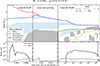 |
Fig. 4. Time evolution of the primary star in model M1, i = 13.5 M⊙, qi = 0.50, and Pi = 6.3 d from the onset of Case B RLOF (left), during core He burning (center), and until the end of the run (right). Top: Kippenhahn diagram. The outermost boundaries are colored corresponding to the most abundant element just below (see legend on the right), and the colored patches are based on the dominating mixing mechanism (see legend on the left). A dashed red line shows the maximum extent of the convective H-burning core during the MS. Bottom: Mass transfer rate (solid) and wind mass loss rate from the primary (dashed). |
4.1.1. Case B mass transfer and subsequent stripping
Both stars evolve effectively as single stars until after the primary reaches TAMS. The primary then expands, filling its Roche lobe and initiating mass transfer. During this phase, most of the H-rich envelope is quickly stripped until nuclear-processed material from the core is exposed. This material, initially part of the convective H-burning core, remains H-rich but is He- and N-enhanced (see Fig. 4). At this point, 8.3 M⊙ of the envelope have been removed, and mass transfer becomes less intense, removing an additional 0.77 M⊙. Mass transfer stops as the primary star ignites He, leaving behind a 0.67 M⊙ envelope and a 3.31 M⊙ He core.
During core He-burning, the He core initially grows to 3.57 M⊙ due to the H-burning shell. Stellar winds also contribute to the erosion of the envelope, which is lost 340 kyr after Case B RLOF. At this point, the primary star is a HeS. Over the remaining phase of core He burning (∼106 yr), the primary star sheds 0.59 M⊙ of its He-rich envelope via winds, reaching core He-depletion with MHe−dep = 2.94 M⊙.
The secondary star spins up to critical rotation during RLOF due to the accretion of angular momentum. The time before the CC of the donor star is insufficient for a significant slow down. The secondary is therefore expected to appear as a Be star, both before and after the CC of the primary.
4.1.2. Case BC mass transfer
Comparison the single HeS models of similar mass shows that the primary star will expand to fill its Roche lobe (7.6 R⊙) roughly 10 kyr before collapse (see Figs. 1 and 2).
Figure 4 shows that 8.7 kyr before CC, the primary began Case BC RLOF, reaching a maximum rate of ∼2×10⁻⁴ M⊙ yr−1 as the first C-burning shell turns off. By the end of core-O burning, RLOF removed about 0.71 M⊙ from the He-rich envelope, which now has a mass of 0.52 M⊙ with an average metal abundance 〈Z〉 = 0.13 (mostly C, N and O).
4.1.3. Case X mass transfer
Following radiative Si-burning, a Ne-burning shell ignites at the outer edge of the CO core, at around a mass coordinate of 1.54 M⊙), developing a thin convective region. This region then merges with the He-rich convective shell above (see Fig. 5), leading to ingestion of He in hotter and denser layers. He is now burnt at higher densities and temperatures, increasing the shell's luminosity, while metal-rich material is dredged-up, raising the envelope's opacity. The envelope becomes fully convective, and the radius expands significantly from 10 to 56 R⊙ in ∼20 d (see Fig. 5). Additionally, 14N is dredged down into the burning shell, triggering the chain 14N(α, γ) 18O(α, γ) 22Ne(α, n) 25Mg which releases free neutrons and likely initiates s-process nucleosynthesis.
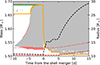 |
Fig. 5. Zoom-in of the Kippenhahn diagram close to the edge of the CO core where the Ne-burning shell ignites at a mass coordinate of 1.54 M⊙ and develops a convective region just above it that then merges with the He-burning shell after about 10 d. The solid lines, and patch colors are the same as in Fig. 4. The dashed lines correspond to the radius (black, dashed), the Roche lobe radius (red, dashed) and the volume-equivalent radius of the outer Lagrangian point (red, dotted). |
The abrupt expansion triggers a new phase of mass transfer, which we refer to as Case X RLOF1. The resulting overflow (R/RRL, 1≃3) is enough to engulf the companion, thus initiating a CE phase. The model sheds 0.60 M⊙ during Case X RLOF, though this is a lower-bound estimate as mass transfer was ongoing at rates of ≳0.1 M⊙ yr−1 when the model terminated. The SN-progenitor would retain a low-mass (<0.13 M⊙), metal rich (〈Z〉>0.5) envelope. With an orbital period of 8 d before Case X RLOF, the remaining time left to CC suggests the primary will likely explode during CE evolution.
4.2. Overview
The binary models rerun in this work evolve similarly to the model in Sect. 4.1. Here, we now discuss the quantitative differences and trends, in the model grid. Each model is labeled “B” followed by its initial primary mass, a “p” and its initial orbital period. For example, B13.5p6.3 refers to the model with M1, i = 13.5 M⊙ and Pi = 6.3d, discussed in Sect. 4.1.
4.2.1. Case B RLOF and envelope loss
All the models in this set undergo Case B RLOF as the first mass transfer event, removing about ∼90% of the primary's envelope mass and leaving behind between 0.55 and 0.83 M⊙ of the H-rich envelope. This phase of mass transfer is stable in all models per our stability criterion (see Sect. 2.4).
After the onset of core He-burning, the remaining H-rich envelope is lost via shell burning and winds within 20% to 70% of the core He-burning lifetime. By the end of core He-burning, models with the same initial masses evolve into HeSs of varying masses (see Table. 2). Losing the H-rich envelope after a significant fraction of the core He-burning phase introduces some differences in the internal structure between single HeS and binary-stripped HeS models, discussed in Appendix B.
The models align in the sHR diagram as a function of their core mass (see Fig. 6). The phase of core He-burning, while long-lived (∼1.2−1.8 Myr), is challenging to observe, particularly in the optical, due to the strong flux from the higher-mass MS companion. Recent UV observations by Drout et al. (2023) reveal HeS companions to otherwise apparently single MS stars exhibiting UV-excess. Some of their observed stars may evolve similarly to our models, depending on the mass and distance of the MS companion.
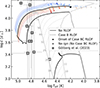 |
Fig. 6. Spectroscopic HR-diagram of the binary-stripped models explored in this work. The models are color-coded by the mass at core He-depletion MHe−dep (see Fig. 3). Each track is plotted from the end of core He-burning until the onset of Case BC RLOF (filled circle). For those that do not undergo RLOF, the plot is shown until the point found at 20 yr before the end of the run (empty circle). The track of model B13.5p6.3 is highlighted in black and shown from ZAMS. The He-stars in the Small and Large Magellanic Clouds analyzed by and Götberg et al. (2023) are also shown (black squares), and numbered as in Drout et al. (2023). |
4.2.2. Case BC RLOF
All but the widest models in the set undergo Case BC RLOF after core He depletion. Although the majority of the models crashed before reaching CC (see Sect. 4.3), the bulk of the mass transferred during Case BC has been captured due to the limited mass transfer rates and the short time remaining before CC. This phase of mass transfer is stable for all models.
The time evolution of the mass transfer rate (see Fig. 7) depends on when RLOF begins. Generally, two phases can be distinguished. A weaker phase (ṀROLF < 10−4 M⊙ yr−1) occurs >5 kyr before CC, and is seen only in the tight systems starting RLOF much earlier. A stronger phase follows, as the envelope expands after the first C-burning shell ignites (between 6 kyr and 1 kyr before CC, depending on mass; see Fig. 1), leading to mass-transfer rates of up to 3×10⁻⁴ M⊙ yr−1. For the systems starting RLOF only in their last 5 kyr, ṀRLOF reaches high rates in the final ∼100 yr before CC. In contrast, those already undergoing RLOF at this time show significantly lower rates closer to CC, and in some cases even detach. For all but the most massive models, mass transfer will terminate ∼20−40 yr before CC, following the ignition of Ne.
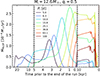 |
Fig. 7. Mass loss as a function of time prior to the end of the run for the set of models with M1, i = 12.6 M⊙ with different initial orbital periods (marked by different colors). The three different panels highlight different timescales. |
Figure 8 shows that the mass-loss during Case BC (ΔMRLOF−BC) scales with how early the star is expected to fill its Roche lobe, determined by comparing the models’ Roche lobe radius with the radius of single HeS models of the same initial mass. Trends in ΔMRLOF−BC align more closely to the single HeS radius evolution when compared using a variable other than MHe−dep (see Appendix B). Mass lost during Case BC RLOF depends on how early the model began RLOF, independently of the HeS mass (see Figs. 8 and B.2.). If RLOF begins 20 kyr, 10 kyr, 5 kyr and 1 kyr before CC, it removes about 0.8 M⊙, 0.6 M⊙, 0.4 M⊙ and 0.1 M⊙ respectively. The stripping only affects regions of the envelope that are still rich in N.
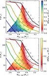 |
Fig. 8. Maps showing the ΔMRLOF−BC (top) and the amount lost after ṀROLF exceeds 10−4 M⊙ yr−1 (i.e., |

4.2.3. Case X RLOF
This phase of mass transfer, previously outlined in Sect. 4.1.3, affects only half of the models, all of which fail to reach CC. Case X RLOF typically reaches mass loss rates of 10−2−1 M⊙ yr−1, removing 0.2−1 M⊙ of material. These values are lower-limits, as the models terminate before CC of the donor. Case X RLOF is always unstable as all models undergo OLOF and, in some cases, the HeS expands enough to engulf the secondary star.
The onset of Case X RLOF is linked to the evolution of the donor star. It typically occurs after the onset of radiative Si-burning and the ingestion of He in the outer core of the donor star. This ingestion leads to the increase in the luminosity of the donor star as well as the envelope opacity, causing the sudden expansion (see Sect. 4.1.3). However, there are some models where the donor star exhibits He-ingestion without expanding. The reason as to why helium is ingested in the first place remains uncertain.
Convective over- and undershooting likely play a key role in this phenomenon, (see Sect. 7.3.2). These methods lack physical backing and were introduced to help with convergence in the calculations. Consequently, we limit our discussion of the effects of Case X on the SN to a more qualitative analysis (see WF22 for a detailed analysis of this phase of RLOF in HeS+NS binaries). To exclude the effects of He-ingestion and Case X RLOF, we use the pre-SN data at 1 yr before the model termination in the following sections.
4.3. Termination and explosion properties
The majority of our models develop a Si-rich core, and only three (B13.815.8, B14.1p10.0, and B14.1p15.8) reach the point of CC. These models provide estimates for the time between CC and specific burning phases: 22−10 yr after core Ne-burning, 10−1 yr after core O-burning, and about 10d after core Si-burning.
Models B12.3p5.01-B12.3p251, B12.3p251, B12.6p5.01 and B12.6p6.31 terminate while burning Ne/O off-center. Of these, B12.3p5.01 (the most-stripped model) exhibits central density and temperature evolution akin to that of a ECSN progenitor (see Sect. 3.1 and Tauris et al. 2015). All other models develop higher temperatures, indicating that they will eventually undergo CC.
We applied the prescriptions from Müller et al. (2016) and Mandel & Müller (2020) to the models reaching CC and obtained explosion energies of Ekin, ej = 5.8−7.0×1050 erg, nickel masses of MNi = 0.03−0.04 M⊙, and NS masses of Mns = 1.34−1.37 M⊙. These values resemble those reported in Ertl et al. (2020) based on the HeS models from Woosley (2019). We investigate the compactness parameter ξm (O’Connor & Ott 2011; Sukhbold & Woosley 2014) of our models at the end of the run (see Fig. 9), and find that ξ2.5 decreases with decreasing MCO, end. This trend aligns with previous studies (e.g., Ertl et al. 2020; Aguilera-Dena et al. 2022, 2023) where also Ekin, ej also decreases to as little as 1.0−1.2×1050 erg. Since all these values are derived from recipes based on 1D-explosion models, they may be uncertain, and we also consider other values for the explosion energy and nickel mass below.
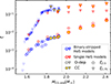 |
Fig. 9. Scatter plot showing the compactness parameter ξm=(m/ M⊙)/(R(m)/1000 km) for m = 1.75 M⊙ (triangle marker) and 2.5 M⊙ (circle marker) as a function of the final CO core. The results of both the single (red) and binary-stripped HeS models (blue) are shown. The compactness is evaluated at core O-depletion for all models (empty markers), including at CC for those that reached it (gold fill). Models with Mend<2.5 M⊙ are shown with lighter colors. |
In the following sections, we adopt a mass Mns = 1.35 M⊙ for the NS, and discuss the effects of the adoption of other values between 1.20 M⊙ and 1.50 M⊙. The ejecta mass of the resulting SNe is given by Mej=Mend−Mns. The composition of the ejecta is also noted, and it is distinguished between He and metals (Mej(He) and Mej(Z) respectively), as shown in Fig. 10.
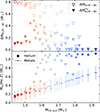 |
Fig. 10. Properties of the primaries as a function of the final CO-core mass of the primary star. The markers are colored as a function of MHe−dep, as in Fig. 3. Top: Amount of mass ejected during Case BC RLOF. The empty markers represent the total mass lost via mass transfer, while the filled markers represent the mass shed during mass transfer after ṀROLF > 10−4 M⊙ yr−1 for the first time. Bottom: Amount of helium (circles) and metals (error bars) found in the ejecta. The uncertainty in the metal content derives from assuming Mns to be within 0.15 M⊙ of the fiducial value (horizontal marker). |
Except for the most heavily stripped models, the ejecta is He-rich (Fig. 10), and we can therefore assume that these will explode as Type Ib SNe. However, simulations of the explosion of low-mass HeS models show peculiar nebular spectra, which do not at present have any observational counterparts (Dessart et al. 2021, 2023). One possible explanation is that they instead lead to Type Ibn SNe (Dessart et al. 2022). The average He content in the ejecta varies significantly depending on the CO-core mass and the degree of stripping. The least massive models at CC (Mend<2.1 M⊙) have comparable amounts of He and metals in the ejecta, within a reasonable deviation of Mns from its fiducial value. The transition to a Type Ic SN also depends on the details of the explosion (e.g. the degree of mixing of Ni in the He-rich regions, as well as asymmetries in the explosion itself, would affect the excitation of HeI lines, Lucy 1991; Dessart et al. 2012; Woosley et al. 2021). More stripped models, with low He and high metal abundances in their ejecta, are more likely to explode as Type Ic SNe.
In the next sections, we solely focus on the CSM interaction features of the SN. The additional effects arising from the ejecta-companion interaction are briefly discussed in Sect. 7.5.
4.4. Post-supernova evolution of the system
Following the SN, intense mass-loss and natal-kicks on the newly born NS (Burrows et al. 1995; Janka 2017) affect the orbital evolution of the system, increasing its eccentricity and even unbinding it. The overall low-mass of the SN progenitors may result in a lower natal kick (Janka 2017). Combined with the relatively short pre-explosion orbital periods, this increases the probability of these systems remaining bound, potentially forming a Be-X-ray binaries (see Sect. 4.1.1).
The secondary is expected to evolve much like a single star until it is close to filling its Roche lobe. Here, mass transfer will likely turn unstable, triggering a CE phase. If the CE is ejected, a tight WD+NS binary may form. Conversely, if the CE is not ejected, the NS will merge with the companion forming a Thorne–Żytkow object. These results can also be extended to systems with more massive secondaries than those presented here (see Appendix A). In such cases, the CE phase may produce a tight HeS+NS binary, where the HeS is massive enough to undergo CC. The resulting SN explosion could exhibit interacting features if Case BC RLOF occurs between the HeS and its NS companion (e.g., WF22). If the natal kick of the newly formed NS does not disrupt the binary, the system forms a double-NS system, which would eventually merge and emit gravitational waves (Qin et al. 2024).
5. Supernova-circumstellar material interaction
All SN-progenitor models that undergo Case BC RLOF explode with a significant amount of H-poor material likely remaining close to the binary system. Here, we discuss the CSM properties from our models (Sects. 5.1 and 5.2), their potential effects on the SN light curve (Sects. 5.3–5.5) and a discussion on the number of interacting H-poor SNe expected from binary models (Sect. 5.6). We do not pursue a discussion of the effect of the CSM on the spectral evolution (but see Dessart et al. 2022), as this depends on strongly non-linear physics and requires detailed radiative-transfer modeling.
5.1. Circumstellar material mass
The upper limit on the CSM mass (MCSM) in our models is given by ΔMRLOF−BC. Some of this mass may escape the system and therefore not affect the SN. Most observations do not track the late-time evolution of the SN, often missing out on the prolonged interaction phase (e.g., Type IIn SNe, Smith et al. 2017). This restricts inferred CSM properties to the closer, denser regions where interaction power dominates the observed light curve.
Our models constrain the total mass lost from the binary but are less predictive of the circumbinary density distribution. To exploit the time-evolution of the mass outflow from the binary model, we computed not only its total amount but also, separately, the amount of mass that was lost during the stronger phase of mass transfer in the last ≲3 kyr before CC (see Fig. 7) as
 (1)
(1)
where t4 is the time during Case BC RLOF such that ṀROLF exceeds 10−4 M⊙ yr−1 for the first time. This quantity is not sensitive to the adopted threshold (see Fig. 7). Unlike ΔMRLOF−BC,  does not correlate with the time the star fills its Roche lobe. Systems that undergo RLOF exclusively within 10 kyr before CC achieve the highest values of
  (see Fig. B.2. and Sect. 4.2.2), and those that begin RLOF even later (≲3 kyr before CC) lose all their mass at high rates, resulting in
  (see Fig. 7).
In Fig. 11, we find a strong anti-correlation between Mej and MCSM when assuming MCSM=ΔMRLOF−BC, which is also present when we extrapolate ΔMRLOF−BC in the whole binary grid. This extrapolation is done by mapping each model in the binary grid onto Fig. B.2. and assuming Mns = 1.35 M⊙. This anti-correlation is driven by the fact that the lower-mass models expand more and therefore lose more mass (see Sect. 4.2.2 and Fig. 8) compared to higher-mass models. The combinations of MCSM and Mej result in different effects on the light curve (background color, Fig. 11) and are discussed in Sect. 5.3.
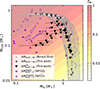 |
Fig. 11. Circumstellar material in our models at the time of the SN, according to various estimates, versus the SN ejecta mass. The CSM mass given by ΔMRLOF−BC (white, with black outline) and |

When assuming  , trends differ only for Mej<1 M⊙, where MCSM decreases with decreasing Mej (see Fig. 11). This is because, even though lower mass models generally lose more mass, the absolute amount lost in the last 5 kyr is proportionally much less than in other systems (see Fig. 7 and the bottom panel in Fig. 8).
5.2. Circumstellar material extension and shape
As we do not model the CSM density structure, we estimated its spatial extension analytically under simple assumptions. For this, we considered two approaches.
In the first approach, we assumed that the CSM consists of a steady spherical outflow with constant velocity vCSM, from which we can infer its extent. For vCSM = 10 km s−1, the CSM would extend to distances of 1015∼1018 cm (see Fig. 12). These distances correlate with the mass of the CSM, with the more extended CSM containing more mass (see Sect. 4.2.2). Most of our mass donors detach from their Roche lobe before CC (except those with MHe−dep>2.90 M⊙ and RRL<30 R⊙), usually by core Ne-ignition. This leaves a cavity, extending to ∼6×1014 cm, filled by donor's stellar wind. This cavity implies that the interaction between the ejecta and the CSM will be delayed by several days, assuming vej∼9000 km s−1. In models that do not detach, mass transfer in the last ∼20 yr deposits ∼0.001 M⊙ of material in that region (Fig. 12).
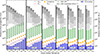 |
Fig. 12. Bar chart of the spatial distribution of material from the SN progenitor models 1 yr prior to the end of the run for the models run in this work. Color bars highlight the envelope (blue filled bar) and the regions where the CSM would be found (hatched bars) if it were distributed along a CBD (green) or if it were expanding isotropically, at a constant speed of 10 km s−1 (gray). In the latter case, the minimum radius is set as the point where the cumulative mass of the CSM from the progenitor star reaches 0.001 M⊙, and increases in contrast when it reaches 0.01, 0.1 and 0.5 M⊙. The Roche lobe radius of the progenitor star is shown (blue hatched-line) as well as the volume-equivalent radius of the outer Lagrangian point (red hatched-line). Finally the companion's location is also shown (orange marker) alongside its Roche lobe (vertical orange hatched-line). The models are grouped by different initial masses (indicated in the bottom of each box). |
Alternatively, material that leaves the binary may accumulate in a circumbinary disk (CBD), if channeled through the outer Lagrangian point of the accretor (e.g., Lu et al. 2023). Whether or not the material remains bound depends on its velocity. Given the high mass-ratio of the systems during Case BC RLOF, material escaping from the outer Lagrangian point with a small perturbation may remain gravitationally bound, feeding the disk. The inner disk radius is expected to be comparable to two to three times the semi-major axis of the binary (Artymowicz & Lubow 1994; Pejcha et al. 2016), corresponding to 1013−1014 cm in our models. The outermost disk radius is limited by photo-evaporation from the radiation emitted by the stars in the inner binary (Hollenbach et al. 1994). For a post-CE binary with M1=M2 = 10 M⊙ in a tight orbit with a = 30 R⊙ and a CSM of 1 M⊙, Tuna & Metzger (2023) find that the CBD extends up to 3000∼10 000 R⊙ (see their Eq. (29) and Fig. 5), that is, about 100–300 times the orbital separation. Adopting the conservative value of 100a as the outermost edge of the disk, we estimate CBDs in our models to extend between 6×1012 cm and 4×1015 cm (see Fig. 12).
We can extend this consideration to the whole binary grid. The final orbital separation for systems undergoing Case BC RLOF is derived by estimating ΔMRLOF−BC (see Sect. 5.1) and integrating Eq. (5) in Willcox et al. (2023) for each candidate model. The resulting CBDs across all models in the binary grid are expected to be found between 3×1012 cm and 1016 cm. The inner boundary of the disk can be between 3×1012 cm to 1014 cm, implying that ejecta-CSM interaction is always delayed, from several hours to up to just above a day, assuming vej∼9000 km s−1.
5.3. Cumulative effect on the light curve
As the expanding ejecta collide with the CSM, a fraction of its kinetic energy will be converted into radiation, thus affecting the SN light curve. Type Ibc SNe show a total radiated energy of ≲1049 erg (Nicholl et al. 2015). For an explosion energy Ekin, ej of 6×1050 erg (see Sect. 4.3), CSM interaction could dominate the typical Type Ibc light curve more than ∼2% of the kinetic energy is converted into light. For Ekin, ej = 1050 erg, more than 10% of Ekin, ej would need to be converted.
Assuming an inelastic collision, the cumulative interaction power can be estimated as (Aguilera-Dena et al. 2018)
 (2)
(2)
where η is the efficiency with which kinetic energy is converted into radiation, and the two multiplicative factors represent the mass  and velocity
  contrasts between the ejecta and the CSM. Assuming that the CSM is slow-moving (fv∼1), and that the conversion is highly efficient (η∼1), the fraction of kinetic energy converted into radiation equals fM, which is only a function of the ejecta mass and the CSM mass.
The value of fM increases with decreasing ejecta mass and increasing CSM mass (see Fig. 11), peaking in the models with the most stripping (∼0.75 if MCSM=ΔMRLOF−BC, and ∼0.45 if  ). Models with less stripping during Case BC RLOF, can still convert as much as 10% of Ekin, ej into radiation if MCSM>0.1 M⊙. For both cases, interaction would convert a significant fraction of the SN kinetic energy into radiation, strongly impacting the SN light curve. It is worth noting that these values of fM are upper limits, as they assume that all the mass remains close enough to the progenitor to affect the light curve.
The low mass-loss rates in our models imply low CSM densities, meaning the SN radiation may not thermalize and therefore not result in an optically luminous transient. Instead, most of the flux would come out in the UV or as X-rays (Dessart & Hillier 2022). Consequently, we focus on the case in which the CSM is distributed along a CBD, where higher densities are achievable. We consider an isotropically expanding ejecta impacting a CSM confined within a half-opening angle θ from the orbital plane. The effective ejecta mass Mej, eff, that is the part of the ejecta that will impact the CSM, is smaller than the total amount Mej and is determined by the solid angle that the CSM subtends:
 (3)
(3)
Recalculating the energy lost due to the inelastic collision, we obtained a similar form to Eq. (2) with
 (4)
(4)
For Mej∼MCSM and θ≪1, then fM(θ)∼θ. The cumulative interaction-power will exceed the typical radiated energy in Type Ibc SNe as long as θ>1° for Ekin, ej = 6×1050 erg, or θ>5.5° for Ekin, ej = 1050 erg. Even for very thin disks, interaction power can dominate the cumulative radiation. In thin disks, high densities may trap radiation, causing it to expand the material rather then escape as radiation. Consequently, our estimates represent upper-limits on radiated energy.
Below, we consider at which time the light curve might be affected the most, based on different assumptions on the CSM structure.
5.4. Interaction light curve for a constantly expanding CSM
We present simplified light curve models, assuming interaction as the sole source of SN luminosity. We neglect diffusion processes and the spatial extension of the ejecta and the swept-up CSM, and focus on the conversion rate of kinetic energy into escaping radiation. The equations are detailed in Appendix C.1.
We use model B12.3p25.1 as our fiducial model, as it shows the strongest mass-loss rate close to CC of all models (3.1 × 10⁻⁴ M⊙ yr−1). The results are shown in Fig. 13. We also assume that the CSM is isotropically distributed.
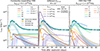 |
Fig. 13. Interaction-powered light curves for model B12.3p25.1 assuming a constantly expanding CSM (left panel) and a CBD-like CSM (right panel). A comparison of the two approaches with different explosion energies is shown in the center panel. In each panel, two observations are shown, namely, the Type Ibn SN OGLE-2012-SN-006 (Pastorello et al. 2015a, light-blue scatter) and the Type Icn SN 2019jc (Pellegrino et al. 2022b, orange scatter) as well as the template light curves for Type Ibc SNe (Nicholl et al. 2015, in violet, where the peak is located at the same time as in the light curve of model he4 from Dessart et al. 2020) and Type Ibn SNe (Hosseinzadeh et al. 2017, in blue, where the peak is arbitrarily placed at 10 d). Left: The CSM is assumed to constantly be expanding at vCSM = 10 km s−1, with different opening angles (with different colors) and with Ekin, ej = 6×1050 erg. For θ = 90°, models with vCSM of 5 km s−1 (dotted line) and 20 km s−1 (dashed line) are also shown. Center: Interaction power from the CBD-like CSM (solid, with Rin = 1013 cm, Rout = 1015 cm, and s=−1) and a constantly expanding CSM (dashed, with vCSM = 10 km s−1) are shown with different Ekin, ej (different colors), assuming an opening angle θ = 10°. Right: The CSM is assumed to be CBD-like, with Rin = 1013 cm, Rout = 1015 cm, s=−1 and different opening angles (different colors). For θ = 5°, the cases with s = 0 (dashed) and s=−2 (dotted) are also shown. |
The interaction luminosity (Linter) becomes significant only after a few days, due to the presence of the cavity in the CSM (Sect. 5.2) which would otherwise be filled by winds which are presently ignored. The light curve also exhibits a plateau after the onset of the interaction, which is qualitatively similar to that obtained in detailed radiative-transfer models in Dessart et al. (2022) for a wind-like CSM. This plateau, which is not usually present in most observed Type Ibn SNe with the exception of OGLE-2012-SN-006 (Pastorello et al. 2015a), arises from the roughly constant mass-loss rate. The ejecta therefore sweep about the same amount of mass per unit time, producing a steady energy conversion rate. The absence of diffusion processes in the model is also gives rise to this peculiar signal, as its inclusion would have altered the luminosity evolution at early times, where the CSM is denser and more optically thick.
The effect of varying vCSM are shown in Fig. 13. Higher vCSM increases the lag time before the onset of interaction and decreases Linter (see Eq. (C.9)) and vice versa. The interaction persists for as long as several years, as the ejecta sweeps material that has traveled since the beginning of Case BC RLOF. However, the optical signal will remain weak and likely become undetectable much earlier than that, as only the innermost CSM is optically thick.
An aspherical CSM distributed along a torus, confined near the orbital plane within a half-opening angle θ, presents a more interesting scenario. Here, only a fraction of the ejecta interacts with the CSM (Mej, eff; see Sect. 5.3), which decreases with smaller θ. At the onset of interaction Linter remains unaffected, as the same amount of mass would be swept up independently of θ. However, smaller θ cause a stronger deceleration of the effective ejecta, reducing Linter at later times (see Eq. (C.9)). Significant effects arise only for very small opening angles (<10°).
Lower Ekin, ej affect the light curve in two ways, due to the slower expanding ejecta: reduced luminosity and delayed onset of interaction (see Fig. 13). As in the model  , the overall luminosity decreases strongly with decreasing Ekin, ej. The onset of interaction is instead delayed by a factor
  . For Ekin, ej≤1050 erg, the interaction luminosity drops to ≲2×1041 erg s−1, and would remain largely undetectable.
5.5. Interaction light curve for a circumbinary disk-like CSM
We now model the interaction assuming the CSM is a bound CBD (such that vCSM = 0) rather than spherically symmetric (see Sect. 5.2). This approach introduces additional parameters and assumptions – such as the half-opening angle θ, the CBD density profile and its radial extent – which are not constrained by our models. We assumed that ρ(r)∼rs, with s≤0, and that the CBD is confined between Rin = 1013 cm and Rout = 1015 cm.
As a proof of concept, we present a simplified light curve model (see Appendix C.2), assuming Ekin, ej = 1050 erg (Fig. 13). The effect of varying θ is more pronounced than in the case of a constantly expanding CSM. For thinner disks, Linter is weaker and dims faster, as less ejecta interacts with the CBD. The characteristic the bell-shape feature, typical of many Type Ibn SNe (see Hosseinzadeh et al. 2017), is qualitatively reproduced. Varying s also has a considerable effect, as a steeper density profile (i.e., lower s) confine the CBD closer to the binary, resulting in a earlier interaction and higher initial Linter (Fig. 13). Even when adopting such a low Ekin, ej, the interaction power is still significant even for θ = 5° where Linter peaks at >2×1042 erg s−1. Unlike the constantly expanding CSM scenario, interaction terminates after ∼70 d, as the entire CBD is swept away.
Adopting Ekin, ej>1050 erg results in a brighter and faster-evolving light curve, similarly to the case of a constantly expanding CSM (see Sect. 5.4, and Fig. 13), as the peak brightness scales with  and the peak time with
  . Models with θ≥10° are capable of exceeding the typical luminosity of Type Ibc SNe, even with Ekin, ej<1050 erg. This model can also qualitatively reproduce the behavior of Type Icn SN 2019jc, especially in the case of thin, confined CBD and higher Ekin, ej.
This experiment, while very crude, demonstrates that a disk-like CSM can significantly shape the light curve, particularly for thin disks, which qualitatively mash some observed Type Ibn and Type Icn light curves. This model, however, neglects radiation transport, which would smear the interaction power on longer timescales, or even reduce the radiated energy if some is used to expand the material in the CBD. The interaction's asymmetry introduces viewing angle effects. In the case of edge-on observations, the light curve may be additionally smeared-out (see Vlasis et al. 2016; Suzuki et al. 2019, in the context of Type II SNe). Finally, a disk-like structure may conflict with the narrow-line emission spectra (Smith 2017).
5.6. Predicting the number of interacting H-poor supernovae
Since we infer the mass-loss during Case BC RLOF from each model in the comprehensive binary grid of models from Jin et al. (in prep., see Sect. 5.1 and Fig. 11), we provide population estimates for the models we predict will develop into an interacting SN. As shown throughout Sects. 5.3–5.5, a significant fraction of the kinetic energy of the ejecta can be converted into radiation when MCSM≳0.1 M⊙. We assume that an interacting H-free SN may likely develop in those systems where the stripped-envelope donor star underwent Case BC RLOF.
We perform a population synthesis calculation, assigning an initial probability distribution to each model in the binary grid from Jin et al. (in prep.) assuming that all stars are born in binaries with a Salpeter (1955) initial mass-function for the initially more massive star and a flat initial log Pi and qi distribution. We also assume that the binaries that undergo unstable RLOF will merge (see Sect. 2.4), and that the merger product will evolve like a single star of the same mass as the sum of the two component stars. We identify SN progenitors undergoing Case BC RLOF by adopting the method shown in Sect. 5.1, and obtain that up to ∼12% of all stripped-envelope SN progenitors will develop into an interacting H-free SN. The observed fraction of Type Ibn SNe reported in Perley et al. (2020) is 9.2%, although this is a magnitude-limited sample and therefore may overestimate the true population of these events. This similarity suggests that binary mass transfer might be a suitable channel to create the majority of interacting H-free SNe.
6. Comparing observed interacting H-poor supernovae with the models
To date, there is a growing number of H-poor SNe that exhibit features compatible with that of interaction with a nearby CSM. The light curve and the spectra provide insight into both the explosion parameters of the SN (Mej, vej, MNi and Ekin, ej) and the properties of the CSM (MCSM, RCSM), albeit under a series of assumptions (see MOSFiT, Guillochon et al. 2018, and also Chatzopoulos et al. 2012, 2013; Villar et al. 2017). These models typically assumed isotropic CSM distributions around the progenitor, with a density profiles of the form ρ(r)∼rs starting at a distance RCSM. Many works usually keep the parameter s fixed to either 0 (a constant distribution) or –2 (wind-like) or explore both, yielding significantly different light-curve fitting parameters (e.g., Ben-Ami et al. 2023). More recent theoretical works have produced Type Ibn SNe by exploding a low-mass He-star model while surrounded by a massive CSM, yielding interesting matches to the light curves and spectra of events like SN 2006jc, SN 2018bcc and SN 2011hw (Dessart et al. 2022).
There is a notable lack of systematic analysis of H-poor interacting SNe. Many studies incorporate additional physical processes, such as Ni decay or magnetar spin-down, that complicate the interpretation of the effects of CSM interaction. Moreover, the discussion in Sect. 5.2 tells us that the CSM may be distributed aspherically, violating the assumption of isotropy used in standard light-curve fitting methods. These modeling uncertainties inevitably affect the interpretation of observations.
In this work we compare our model predictions with published observationally inferred properties of H-poor interacting SNe, without making claims about any specific observed event. It should be emphasized that we use literature values without assessing their accuracy or robustness. Some of the values, especially from older studies, may be inaccurate.
We searched the literature for H-poor interacting SNe and included only those for which MCSM values are available. In the following, we discuss Type Ibn SNe (Sect. 6.1) and Type Icn/Ic-CSM SNe (Sect. 6.2).
6.1. Type Ibn supernovae
The sample of Type Ibn SNe includes H-poor and He-rich transients that showcase narrow He-emission lines. The sample spans a wide range of Mej (between 0.6 and 20 M⊙), and MCSM (between 0.01 and 2 M⊙). Most SNe in the sample cluster around Mej∼1 M⊙ and MCSM between ∼0.1 and 1 M⊙. Despite their large uncertainties, these values align with the parameter space predicted by our models (see top-left panel of Fig. 14), regardless of whether MCSM corresponds to ΔMRLOF−BC or  . Some SNe fall outside of the predicted MCSM−Mej region (SN 2006jc, SN 2010al, ASASSN-14ms, SN 2020bqj, SN 2019uo). These outliers, characterized by high Mej, likely originate from a different evolutionary channel.
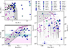 |
Fig. 14. Comparison between model data and parameters inferred from observed Type Ibn SNe (blue-scale colored markers). The different markers are associated with different SNe, and different colors for the same SN highlight different references. Estimates inferred from the models of WF22 are also included and are shown as in Fig. 11. Top left: Scatter plot showing the amount of mass of the CSM against the ejecta mass in the models as in Fig. 11. As the values of MCSM from the models is an upper limit, a light-gray region is added where models can still be expected. Right: Scatter plot showing the extent of the CSM against its mass. The position of CBD-like CSM from our models is shown with a gray line for MCSM=ΔMRLOF−BC. The region where CBDs from the models in the binary grid are expected to be found is shown with a vertically hatched region. The radii of our theoretical model are also shown (cross scatter). A gray patch is drawn where to expect the CSM if it were to move constantly at a speed of 10 km s−1. Bottom left: Scatter plot showing the energy released by interaction (Eq. (2)) as a function of CSM mass for the models in this work and WF22 assuming Ekin, ej = 6×1050 erg (shown with a black horizontal line) and the total light-curve energy of the observed SNe. The shaded regions represent the typical Erad of Type Ibc (light-red, Nicholl et al. 2015) and Type Ibn SNe (light-blue, Hosseinzadeh et al. 2017). The values expected from our models and those in the binary grid are summarized in gray regions, which also show the expected Erad if MCSM is lower than the values inferred. Each gray region assumes that the CSM is distributed spherically (solid line, light-hatch), along a CBD with θ = 15° (dashed line, dense hatch) and 5° (dotted line, gray fill) of the orbital plane (see Eq. (4)). References: SN2006jc: (1) Mattila et al. (2008), Pastorello et al. (2007); (2) Tominaga et al. (2008), Pastorello et al. (2007); (3) Chugai (2009), Pastorello et al. (2007); (4) Dessart et al. (2022), Pastorello et al. (2007); SN2010al: (5) Chugai (2022); SN2011hw: (6) Dessart et al. (2022), Pastorello et al. (2015b); LSQ13ddu: (7) Pellegrino et al. (2022a), Clark et al. (2020); (8) Clark et al. (2020), Brethauer et al. (2022); ASASSN-15ms: (9) Vallely et al. (2018); iPTF15ul: (10) Pellegrino et al. (2022a), Hosseinzadeh et al. (2017); SN2018bcc: (11) Dessart et al. (2022), Karamehmetoglu et al. (2021); (12) Karamehmetoglu et al. (2021); SN2018gjx: (13) Prentice et al. (2020); SN2019uo: (14) Pellegrino et al. 2022a; Gangopadhyay et al. 2020; (15) Gangopadhyay et al. (2020); SN2019deh: (16) Pellegrino et al. (2022a); SN2019kbj: (17) Ben-Ami et al. (2023); SN2019wep: (18) Pellegrino et al. (2022a), Gangopadhyay et al. (2022); SN2020bqj: (19) Kool et al. (2021); SN2020nxt: (20) Wang et al. (2024); SN2021jpk: (21) Pellegrino et al. (2022a); SN2022ablq: (22) Pellegrino et al. (2024); SN2023fyq: (23) Dong et al. (2024); SN2023tsz: (24) Warwick et al. (2025). |
The typical inferred CSM extension for Type Ibn SNe exceeds 1014 cm (see Fig. 14, right panel), consistent with the CBD-like CSM expected from the models. Notable exceptions include SN 2020bqj, whose inferred CSM extent is similar to the radii of our SN-progenitor models, and SN 2006jc (>1016 cm), which appears to be instead in agreement with the case of a slow-moving CSM.
The majority of the Type Ibn SNe collected deviate from the Type Ibn template of Hosseinzadeh et al. (2017) as reflected in their the total radiated energy in the light-curve Erad (see Fig. 14, bottom-left panel). Most SNe from Hosseinzadeh et al. (2017) lack MCSM estimates and were therefore excluded from our sample. The collected SNe show a large spread of Erad, with most having a higher value than inferred from the template Type Ibn SNe, and only a few with significantly lower values (SN 2018gjx and SN 2020nxt), which may be the effect of a shorter observation campaign or poor multi-band coverage.
The radiated energy from the models scales with the explosion energy Ekin, ej and decreases with very small half-opening angles (see Eqs. (2)–(4)). The observations with the higher Erad and MCSM align with our models assuming Ekin, ej = 6×1050 erg and a spherically distributed-CSM (see Fig. 14, bottom-left panel), although, they can still be explained assuming a lower Ekin, ej or a CBD-like CSM with θ≥15°. Dimmer events are consistent with significantly lower explosion energies (Ekin, ej∼1050 erg), which are expected in the models with stronger mass-loss and hence smaller final core masses (Sect. 4.3) as well as a thinner CBD-like CSM, with θ≲5°.
The progenitor and CSM properties inferred from the observed Type Ibn SN we collected appear to be consistent with the CBD-like CSM surrounding the binary models explored in this work. However, challenges remain regarding narrow-lines observations. As the narrow lines would originate within the disk, which is likely engulfed by the freely expanding ejecta in the other directions, the narrow-line component would likely be thermalized and therefore unobservable (Smith 2017).
6.2. Type Icn and Ic-CSM supernovae
The observed Type Icn/Ic-CSM SNe feature a diverse sample of events, from the very stripped SN 2023emq (Mej∼0.3 M⊙) to the massive Wolf-Rayet progenitor of SN 2010mb (Mej>10 M⊙). Interestingly, the sample shows a possible correlation between Mej and MCSM, with Mej∼4MCSM (see Fig. 15, upper-left panel), though this be a result of the low number of observed events. SNe with Mej≲1.5 M⊙ align with our models if  (and also ΔMRLOF−BC for those that also have Mej≳1 M⊙). The ones with higher ejecta and CSM masses (i.e., SN 2010mb, SN 2021ckj, and SN 2022ann) cannot be explained by our models.
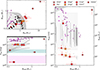 |
Fig. 15. Same as Fig. 14 but for Type Icn SNe and the Type Ic-CSM SN 2010mb. References: SN2010mb: (1) Ben-Ami et al. (2014), Brethauer et al. (2022); SN2019jc: (2) Pellegrino et al. (2022b); SN2019hgp: (3) Gal-Yam et al. (2022); (4) Pellegrino et al. (2022b), Gal-Yam et al. (2022); SN2021csp: (5) Pellegrino et al. (2022b), Perley et al. (2022); SN2022ann: (6) Davis et al. (2023); SN2023emq: (7) Pursiainen et al. (2023). |
The CSM radii in Type Icn SNe are more uncertain than Type Ibn SNe. For example the CSM is inferred to extend from close to the progenitor (∼1 R⊙ in SN 2021csp, Pellegrino et al. 2022b) to 1015 cm (SN 2019hgp, Gal-Yam et al. 2022). For some of these SNe, the adoption of different assumptions in the light-curve modeling changes the value of RCSM by about one order of magnitude (e.g., SN 2019jc, SN 2019hgp ad SN 2021csp; see Fig. 15, right panel), while Mej and MCSM are not affected by more than a factor of two. The inferred CSM extension in these SNe is compatible with either an extended envelope or a CBD. The slow-moving CSM model can, instead, be ruled out.
The radiated energy of these SNe varies significantly. Brighter events, (e.g., SN 2019hgp, SN 2021csp), align with our models assuming a spherically symmetric CSM, as well as a CBD-like structure with θ>20°. The underluminous event SN 2019jc (Pellegrino et al. 2022b) is also consistent with our models when considering lower Ekin, ej and a CBD-like CSM with small opening angles.
Similar to the collected Type Ibn SNe, some Type Icn SNe are compatible with the binary channel proposed and a CBD-like CSM structure proposed in this work. However, explaining their spectral evolution remains challenging, especially as the CSM of all our models is He-rich. While there are models with very low He in the ejecta (≲0.2 M⊙; see Fig. 10), the metal-rich lines would likely appear broad rather than narrow.
Summary
Our models indicate that Case BC RLOF can produce progenitors and CSM structures broadly consistent with those inferred for a subset of the observed Type Ibn, especially when considering a CSM distributed along a CBD. While our models struggle to fully account for Type Icn/Ic-CSM SNe, the similarities in bulk properties (especially MCSM, Mej and RCSM) and light curves (see Sect. 5.5) warrant further investigation of the spectral evolution in progenitors like those presented in this work.
Caution is warranted when interpreting these results. The CSM mass predicted by our models represents an upper limit, while observational estimates are biased toward a spherically symmetric distribution, which our models disfavor. These discrepancies highlight the need for further investigation of the CSM structure and the interaction features it produces, particularly in the case of a CBD-like configuration.
6.3. Comparisons with Case X RLOF
If the progenitor underwent Case X RLOF, the SN would occur while the system is embedded in a H-poor, He- and metal-rich CE (see Sects. 4.1.3 and 4.2.3), which would likely form the CSM. The CE's impact on the light curve would be significant (as fM∼1), likely turning the SN into a SLSN. The CSM structure will be qualitatively different from that generated during Case BC RLOF, due to its more dynamic nature and the shorter timescale before CC.
Case X RLOF has been investigated systematically in WF22 for HeSs with NS companions, assuming that it provides either a stable or an unstable phase of mass transfer. The timescales for Case X RLOF differ significantly between their models and our own: in WF22, Case X RLOF begins even decades before CC, whereas in our models it is confined to only a few weeks or months. We compare their results with the observed Type Ibn and Icn SNe (see Figs. 14–15). Their stable Case X scenario predicts MCSM of up to ∼0.3 M⊙ and 0.1 M⊙≲Mej≲1 M⊙, which is consistent with several observed Type Ibn and Icn SNe with Mej≲1 M⊙ and MCSM<0.3 M⊙, but falls short to explain the bulk of the Type Ibn observations with higher MCSM. The unstable Case X scenario, which yields MCSM of up to ∼1 M⊙ and 0.1 M⊙<Mej<0.4 M⊙, appears incompatible with most observations, due to the very low predicted ejecta masses in that case.
WF22 provide values for RCSM assuming vej equal to the orbital velocity of the L2 point, usually between 100 and 500 km s−1. As a result, their constantly expanding CSM is comparable in size to that of a CBD-like CSM from Case BC RLOF in our models (see Figs. 14–15) and also many observations of Type Ibn SNe (as also discussed in their Sect. 3.5). On the other hand, The CSM geometry may be more complicated than that expected from our models during Case BC RLOF, especially if Case X RLOF is unstable.
The numerical settings used in WF22 are similar to our own, suggesting that their models may also be affected by numerical issues that give rise to this phase of RLOF (see Sect. 7.3.2 for a discussion).
7. Discussion
The results from the models show a series of features that are highly dependent on the assumptions made. We discuss the main uncertainties affecting our result and provide comparisons to previous works.
7.1. Winds and metallicity
The evolution of the models discussed is strongly influenced by the adopted wind scheme. For HeS mas-loss rates, our models use the prescription from Yoon (see Jin et al. 2024), which combines empirical rates of observed Wolf-Rayet stars with higher luminosities than those found in our models (log L/ L⊙>4.90 from Nugis & Lamers 2000; Hamann et al. 2006; Hainich et al. 2014; Tramper et al. 2016, against the maximum luminosity before Case BC RLOF in our models of log L/ L⊙ = 4.75). This raises the question about the validity of our choice of wind recipes.
Recent studies like Vink (2017) argue for lower mass-loss rates for low-mass HeSs. Gilkis et al. (2019) show that this wind mass-loss rate actually prevents the complete loss of the H-rich envelope if adopted when Xs drops below 0.4. This contrasts with the higher rates predicted by Nugis & Lamers (2000), which our models adopt. Additionally, Götberg et al. (2023) suggest that the winds of some HeSs observed in the Small and Large Magellanic Clouds (Drout et al. 2023) are comparable to, or even lower than, those described in Vink (2017).
Significantly weaker winds following Case B RLOF, as would occur with lower initial metallicity, shift the parameter space for Case BC RLOF toward systems with lower initial masses (see Sect. 3), because the core remains more massive. A key consequence of weaker winds is that the H-rich envelope may not be completely removed by core He-depletion. This thin H-rich envelope may be extended enough to also increase the probability of Case BC RLOF (Yoon et al. 2017). The shift to lower initial masses and the larger radii increase the population of interacting SNe, which are nonetheless expected to appear as a Type IIb SN with narrow H-lines if Case BC RLOF fails to strip the remaining H-rich envelope.
Binary models at lower metallicity also fail to lose the H-rich envelope completely (Yoon et al. 2017; Laplace et al. 2020), due to the reduced winds. In some cases, RLOF may occur before core He-exhaustion (Klencki et al. 2022), which can be followed again by Case BC RLOF to further strip down the envelope.
The shift to lower metallicity offers, on the one hand, similar effects as those expected when decreasing the wind, namely that the parameter space for Case BC systems would shift toward lower initial masses. However, there are other metallicity-related effects, such as the changes to the radius evolution, that may reduce the parameter space for Case BC systems. Such effects require detailed calculations to assess the metallicity-dependence of Case BC RLOF and hence the population of interacting SNe.
7.2. Mass transfer
7.2.1. Mass accretion and angular-momentum loss
The amount of mass accreted by the companion star during mass transfer and the amount of angular momentum carried away by unaccreted material are critical parameters influencing the evolution of mass-transferring binaries (Podsiadlowski et al. 1992). We report the key effects on our models, and we refer to (Ercolino et al. 2024, and references therein) for a more detailed discussion.
Angular momentum losses may exceed those accounted for in our models due to additional mechanisms. For example, outflows from the outer Lagrangian point of the accretor, that may occur when mass transfer rates exceed 10−4 M⊙ yr−1 (Lu et al. 2023), can carry away significant angular-momentum. Furthermore, unaccreted material remaining in the vicinity of the system can exchange angular momentum with the inner binary. In the presence of a CBD, additional processes such as mass re-accretion, angular momentum exchanges and eccentricity pumping may also occur (e.g., Wei et al. 2024; Valli et al. 2024). Higher angular momentum losses would tighten the orbit during RLOF and therefore remove more mass from the donor star.
For Case B RLOF, increase angular momentum losses would result in smaller MHe−dep and RRL, 1, which would increase the parameter space for Case BC RLOF. However, this would also make mass transfer more prone to becoming unstable (Willcox et al. 2023). In the context of Case BC RLOF, these effects will likely lead to more mass-loss and therefore larger MCSM. In this case, however, the stability of mass transfer would likely remain unaffected due to the significantly more massive companion and contained mass-loss.
Our models may also underestimate the amount of mass accreted by the secondary (Vinciguerra et al. 2020). Increase in mass transfer efficiency would remove more mass from the donor (e.g., Claeys et al. 2011), expanding the parameter space for Case BC RLOF to occur as well as increasing the likelihood of mass transfer turning unstable (Braun & Langer 1995; Schürmann & Langer 2024). Increased accretion efficiency would reduce the amount of CSM as more of the transferred mass would be deposited on the companion star, rather than lost from the system.
7.2.2. Stability of mass transfer
Even though the computation of mass transfer proceeds unimpeded, special care is required to ensure the results have a physical significance. This includes verifying whether the underlying assumptions hold during the calculations (Temmink et al. 2023) or determining if the system enters an unstable phase of mass transfer. The criteria for identifying unstable mass transfer remain debated and we discuss a few in the context of Case B and Case BC RLOF below. We do not discuss the effects on Case X RLOF here (but see Sect. 4.2.3).
Our calculations assume that unaccreted material is ejected as a fast wind from the secondary star (Soberman et al. 1997). However, there is a limited understanding of how the unaccreted material escapes the inner binary. If it is not ejected efficiently, it may exert drag and extract orbital angular momentum, driving the system into an unstable phase of RLOF.
Marchant (2017) proposes that the unaccreted material can be ejected via a radiation-driven wind, which defines an upper limit on the mass transfer rate Ṁhigh. This rate represents the threshold above which the combined luminosity of the two stars is not able to drive the material away radiatively. The unaccreted material is assumed to lie on the outer edges of the accretion disk at a distance RRL, 2 from the secondary star, and the limit is given by
 (5)
(5)
where M2 is the mass of the secondary, and L1 and L2 the luminosities of the primary and secondary stars respectively. If mass transfer is inefficient and ṀROLF > Ṁhigh, the system cannot remove the unaccreted material from the inner binary, leading to unstable RLOF. Figure 16 illustrates a slice of the parameter space of Case BC systems at M1, i = 12.6 M⊙, revealing that many systems but those with high Pi or qi would undergo CE evolution during Case B RLOF. This is because during Case B RLOF the donor star temporarily dims as it is thrown off of thermal equilibrium. Unless the binary is wide or the companion is very luminous, this instability criterion is met. In our models, where qi = 0.5, are always flagged as unstable according to this criterion.
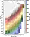 |
Fig. 16. Plot of the log Pi−qi diagram for the Case B binary models in the binary grid from Jin et al. (in prep.) with M1, i = 12.6 M⊙. The color coding is based on the amount of mass expected to be shed during Case BC RLOF. The hatching indicates models that are flagged as having undergone unstable Case B RLOF according to the criterion from Marchant (2017) (single hatch), Pauli (2020) (cross hatch), and Pavlovskii & Ivanova (2015) (circle hatches). |
Pauli (2020) argues that during the short timescale in which the primary star dims, the material can still be pushed away from the inner binary to a finite distance from the system before the primary resettles to a higher luminosity. This may subsequently enable the radiation-driven ejection of the material. They argue that in Eq. (5), L1 should be replaced by the maximum luminosity reached by the donor during mass transfer. This makes the criterion less stringent than that of Marchant (2017), classifying only the models with the lowest qi and Pi as unstable during Case B RLOF. In our rerun models, this affects only the models with Pi<10 d.
Figure 16 highlights the systems expected to undergo Case BC RLOF. Using the stricter criterion from Marchant (2017) significantly reduces the parameter space for the binaries that survive Case B RLOF. For instance, in the grid at M1, i = 12.6 M⊙, most models predicted to experience Case BC RLOF (which give rise to H-poor intreacting SNe) would instead have undergone unstable Case B RLOF and likely merge (likely producing a Type II SN progenitor). By contrast, the criterion from Pauli et al. (2022) only excludes a handful of systems. Both criteria flag more systems as stable with increasing M1, i due to the higher luminosities.
Another indicator of the onset of unstable RLOF is when the donor star swells to the point of undergoing OLOF (Pavlovskii & Ivanova 2015; Ercolino et al. 2024). In this case, the results in the binary grid differ from the binaries we rerun. Due to the inclusion of radiation pressure in the mass-transfer scheme (see Sect. 2.4), the donor stars in our models do not expand as much as those in the binary grid during Case B mass transfer and therefore do not exhibit OLOF, even in cases where OLOF is flagged in the models from the binary grid. Case BC RLOF is never flagged as unstable per the criterion from Pavlovskii & Ivanova (2015).
Our analysis demonstrates that applying different mass transfer stability criteria to the same 1D simulations significantly alters the predicted outcome, particularly for the first phase of mass transfer (i.e., Case B RLOF in these systems, and a similar discussion also holds for those undergoing Case A RLOF). Conversely, Case BC RLOF is consistently stable across all the criteria mentioned, as the mass-loss rates are much lower, the donor does not expand significantly, and the mass ratio is inverted.
7.3. Uncertainties in the latter evolutionary stages
7.3.1. Pre-supernova outbursts
Precursors to the SN explosion have been observed for some interacting SNe (e.g., Strotjohann et al. 2021). Among Type Ibn SNe, pre-explosion outbursts have been observed for SN 2006jc (Pastorello et al. 2007), SN 2019uo (Strotjohann et al. 2021), and SN 2023fyq (Brennan et al. 2024; Dong et al. 2024). It is not yet clear if these outbursts are characteristic of all Type Ibn progenitors. In some cases, pre-explosion photometry rules out the presence of bright precursors, like SN 2015G (Shivvers et al. 2017), SN 2020nxt (Wang et al. 2024), and SN 2022ablq (Pellegrino et al. 2024).
These outbursts may drive intense mass-loss, providing an alternative mechanism to produce the nearby CSM observed in many Type Ibn SNe (Dessart et al. 2022; Maeda & Moriya 2022; Takei et al. 2024). Simulations of SNe with progenitors similar to those in this work were carried out by Dessart et al. (2022), where they included a CSM formed by an eruption in the last ≲2 yr before CC. They find that an outburst-driven CSM leads to light-curve and spectral features compatible to observations of Type Ibn events.
Lower-mass models can experience Si-flashes (Woosley & Heger 2015; Woosley 2019) that release sufficient energy to expand, or even unbind, parts of the envelope. This expansion may also be triggered by Ne-flashes (Wu & Fuller 2022b). In Woosley & Heger (2015), these flashes impact models with MCO, end<1.68 M⊙, which correspond to about half of the models investigated here. While our models lack the proper physics to account for this effect, we argue that the sudden expansion alone can trigger Case X RLOF and create a close-by and dense CSM, perhaps even accompanied by an observable pre-SN outburst.
7.3.2. He/CO shell merger and Case X RLOF
One peculiar behavior that arises in some of our models (and is also found in in the literature, e.g., Tauris et al. 2013, 2015; Wei et al. 2024; Guo et al. 2024, and, more interestingly, WF22) is the presence of a final mass transfer event, which we label as Case X RLOF, shortly before CC. As noted in Sects. 4.1.3 and 4.2.3, this phase of mass transfer is commonly linked to the He-burning shell digging significantly inside the CO core, which is also observed in more massive models in the literature (e.g., Wu & Fuller 2021).
We argue that this phenomenon is likely caused by the use of overshooting in the model. To test this, we ran the model discussed in Sect. 4.1 from the time of core O-depletion, and deactivated overshooting. The following evolution in terms of the development of the subsequent shells is similar, with some slight differences. We focus exclusively on the effects close to the outer edge of the CO core.
As noted already in Sect. 4.1.3, Ne begins burning at a mass coordinate of 1.54 M⊙ roughly a month prior to the end of the run, and it develops a convective region on top of it. This region extends above the Ne/O rich region (which extends up to 1.59 M⊙), thus including the meshes that still retain residual C up to close to the interface with the He-burning shell. Here, differently from the original model, He is not ingested inside this convective region, and the envelope's composition and extension remain unaltered (see Fig. 17). At the onset of convective Si-burning, this convective region dies off.
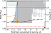 |
Fig. 17. Same Kippenhahn plot shown in Fig. 5 for model B13.5p6.31 (Sect. 4.1) that was reran from core O-depletion without any overshooting. The zero point in the x-axis is set to the onset of convective core Si-burning. The black arrow shows the moment when core Si-burning ends. |
This model showcases two main differences with the original one showed in Sect. 4.1. Not only did the shell merger not occur, but the lifetime of the model also changed dramatically. The original model, following the onset of this external Ne-burning region, would have to wait for another ∼200d to ignite Si convectively, as the core's internal structure is affected following the sudden mass-loss and core-erosion. Without these sudden changes to the stellar structure, convective Si burning begins only two weeks after the onset of the Ne-burning shell close to the outer edge of the CO core, and the model even reaches core-Si depletion, just 11 days after.
In this section we show that the implementation of over- and undershooting is the direct cause for the anomalous behavior experienced in the model. We caution that it remains to be seen if these results also hold in the case of models with a different nuclear network, as the shell structure would change. It is, however, important to mention that the general phenomenon of shell mergers appears in 3D-hydro simulations (e.g., between the C and Ne/O shells in Yadav et al. 2020) and therefore warrants further study.
Regardless of the cause of Case X RLOF, it has already been present in previous models in the literature, though with different features and timescales, such as WF22 and Guo et al. (2024) for HeS+NS systems. In their models, no shell merger is mentioned to occur, and yet a final phase of mass transfer ensues nonetheless about ∼10−50 yr prior to core Si-ignition and the onset of an EC-SNe respectively. Other models have exhibited a similar He/C shell merger, such as Habets (1986) and Woosley et al. (1995), without necessarily exhibiting this expansion phase. This may then indicate that the shell merger we observed in the models is perhaps one of many symptoms that can cause the radial expansion and thus Case X RLOF.
7.4. Circumstellar material geometry surrounding a binary
The structure of the CSM in our models depends on the mechanism that drives the ejection of unaccreted material. If the material is lost through isotropic re-emission (Soberman et al. 1997), it would distribute evenly in all directions. Alternatively, if it is lost through the accretor's outer Lagrangian point, it may accumulate near the orbital plane (e.g., Lu et al. 2023) and form a bound CBD. Such a disk could retain a significant fraction of the unaccreted mass (at least 80% of the mass lost during Case BC RLOF, Pejcha et al. 2016). The presence of such a massive CBD will also introduce a complex shock geometry, particularly at the boundary regions of the disk.
The recent work of Tuna & Metzger (2023) offers an analytical description of the CBD's evolution but for the case of a post-CE CBD. While the evolutionary history of disks in our models differ, their findings offer relevant insight. They suggest that the CBD may persist for ∼50 kyr, with most of its mass lost through re-accretion onto the inner binary, while only a small fraction is lost by photo-evaporation (Hollenbach et al. 1994). In contrast, in our models, the CBD would be continuously supplied with mass by the inner binary. The extension of the CBD – which is determined by the region where photo-evaporation dominates – depends on parameters of the inner binary such as its mass and total luminosity, as well as composition and temperature of the disk (Tuna & Metzger 2023), which we have neglected here.
While we assume that the CSM is entirely contained within a CBD or freely expanding in all directions, the reality is likely more complex. It is reasonable to expect that, while the binary loses material to form a CBD, a fraction of the material can be lost through other mechanisms (e.g., isotropic re-emission, Soberman et al. 1997) resulting in a multi-component CSM. Thus, while the assumption that the RLOF-induced CSM impacts the SN is reasonable, significant uncertainties remain about its mass, extent, and geometry.
Low-mass HeS with high L/M ratios are expected to be pulsationally unstable (Saio et al. 1984; Gautschy et al. 1990; Gautschy & Saio 1995). This is due to the expansion following core He depletion where the outer regions of the envelope experience HeII recombination and become locally super-Eddington, producing a density inversion. These pulsations could trigger episodic phases of mass transfer, as the star would periodically fill the Roche Lobe, therefore losing more mass and further increasing its L/M. Thus, these pulsations could produce a more mass loaded CSM similar to what is expected in the case of a wide RSG+MS mass-transferring binary (Ercolino et al. 2024).
7.5. The effect of a close main-sequence companion on the supernova
The presence of a close-by MS star at the time of the explosion may affect the SN, as the ejecta rams with the companion star. While this has been predicted in the context of Type Ia SNe (see Liu et al. 2023, for a review), one of the first observations hinting at this process for CCSNe was recently reported for the Type Ic SN2022jli (Moore et al. 2023; Chen et al. 2024). The peculiarity of this object lies in the 12.4 d modulation of the light curve. The extended observations presented in Chen et al. (2024) showcase an abrupt decline in the light-curve luminosity (after ∼300 d), which they argue is compatible with a shortl-lived phase of mass transfer between the MS companion, thrown off of equilibrium by the impacting ejecta, and the newly formed compact object gulping material during the passage at periastron.
Since all of our SN progenitors are in orbit with an MS companion, this effect may be present for the tighter systems at CC. In our models, the companion typically subtends up to 1% of the field of view. Assuming an explosion energy of ∼6×1050 erg, the secondaries may capture as much as ∼6×1048 erg of energy, of which only ∼10% may be injected inside the stellar structure to drive its expansion (see Hirai et al. 2018; Hirai 2023, the remaining is instead injected onto the unbound material, which may be as much as ≲0.01 M⊙). If we apply these estimates to the empirical model fits in Ogata et al. (2021), the companion may swell to as much as ∼1000 R⊙, with a very short-lived expansion of at most a few years, which is of the same order of magnitude as the timescale for the luminosity drop in SN 2022jli (Chen et al. 2024).
As the impact with the MS companion will unbind some of its H-rich envelope (Liu et al. 2015; Hirai et al. 2018), we expect that the SNe from our models should showcase narrow H-line emission at late times in the evolution of the SN.
7.6. Comparison to previous works
The mass transfer phase we focused on in our models (Case BC RLOF) results from the expansion of low-mass HeS, a phenomenon well-documented in the literature (Paczyński 1971; Habets 1986; Tauris et al. 2013, 2015; Kleiser et al. 2018; Woosley 2019; Laplace et al. 2020), which our models replicate qualitatively well. Many previous studies of HeSs undergoing RLOF focused on systems with a compact object companion (NS or BH) following a phase of CE evolution (e.g., Dewi & Pols 2003; Tauris et al. 2013, 2015; Jiang et al. 2021, 2023; WF22; Wei et al. 2024; Guo et al. 2024; Qin et al. 2024). In such HeS+NS binaries, the mass ratio during Case BC RLOF is typically <0.5, which is significantly lower than our systems. As a result, their orbit shrinks during RLOF, whereas ours expands, leading to more mass being transferred overall (see also Appendix A). For the HeS+NS systems mentioned above, typical orbital periods are in the order of a few days or less, which can allow the HeSs to fill their Roche lobes during or immediately after core He burning, allowing for more overall stripping than in our models. Such a tight binary with instead an MS companion do not emerge in the binary grid (Sect. 3.2).
One work that modeled RLOF between a HeS and an MS companion was Habets (1986). In their work, RLOF occurs in a very tight orbit (MHeS = 2.5 M⊙, RRL, 1 = 1 R⊙, M2 = 17 M⊙), in the last ≲3 kyr before core Ne-burning, which removes about 0.3 M⊙ of the HeS's envelope. This is much less than what we expect from our models (our models would undergo RLOF ≳20 kyr before CC and therefore remove about 0.8 M⊙; see Fig. 8 and Sect. 4.2.2). Such discrepancy from our models’ radius evolution is to be expected since they adopt older opacity tables and different assumptions for convective mixing, namely that it is instantaneous and that its boundary is defined with the Schwarzschild criterion.
One of our main concerns from our method was the adoption of a limited nuclear network (see Sect. 2.2), especially during the final evolutionary phases. Prior studies in the literature that have adopted larger nuclear networks during Case BC RLOF show results broadly consistent to ours (e.g., Jiang et al. 2021, 2023), with some even showcasing Case X RLOF (Wei et al. 2024; Guo et al. 2024). In Jiang et al. (2021, 2023), where they studied HeS+NS/BH binaries with an detailed nuclear network, mass transfer rates in the last months prior to collapse (i.e., Case X RLOF) were noted to be sensitive to some solver flags (their models, however, do not reach rates comparable to the extreme ones of our models). They were able to derive the SN-explosion properties from their least massive model, which yielded an explosion energy of 6×1050 erg and a remnant mass of 1.34 M⊙. These values are compatible with the ones adopted in this paper (see Sect. 4.3).
8. Conclusions
In this work, we have investigated a comprehensive set of binary evolution models. We focused on those in which the primary is stripped to become a helium star after core hydrogen depletion and undergoes a second mass transfer phase with an MS companion after core helium exhaustion up until close to CC. The later phase of mass transfer is triggered in the systems where the helium-star primary has a mass of less than 3.4 M⊙ by the time of core He-depletion. During this phase, the amount of mass lost depends on how early mass transfer begins, which can remove as much as 0.8 M⊙ of the He-rich envelope for the models that started about 20 kyr before CC.
In our binary models, the MS companion does not accrete significant amounts of the transferred material, which instead is lost from the system to form a nearby H-free circumbinary medium. Its typical mass of 0.4 M⊙ is large enough to give rise to significant interaction features, especially by extracting kinetic energy from the impacting SN ejecta, which can be as high as 70%. Using a simplified model that neglects diffusion, we explored the impacts of different structures of the circumbinary material on the SN light curve. A circumbinary disk-like structure qualitatively reproduces the light-curve morphology of many Type Ibn SNe.
We find that our models produce masses and radii of the circumbinary material as well as ejecta masses and integrated bolometric luminosities that are compatible with those observed in many Type Ibn SNe. However, studies on individual supernovae mostly assume a spherical distribution of the material (see Sect. 6), while our results show that a disk-like distribution is another reasonable possibility. Future studies on the evolution of the circumbinary material produced by binary mass transfer will be crucial to addressing the structure and geometry of the material at CC. This simultaneously calls for future research to explore how these large-scale asymmetries influence the light curve and spectral evolution of interacting SNe and how these factors impact inferred properties from the observed data.
Finally, we developed a method to map the properties of a binary model at core He-depletion to the amount of mass being transferred during the later phase of mass transfer. Applying this method to a comprehensive grid of binary models, we found that 12% of all stripped-envelope SN progenitors produced in binaries are expected to undergo mass transfer until CC and can therefore be expected to become H-poor interacting SNe, which is in broad agreement with observational rate estimates of Type Ibn SNe (Perley et al. 2020). Future observations from ongoing surveys such as ZTF and the beginning of the science operations of LSST in 2025 will yield more significant constraints on the observed population of these SNe.
Acknowledgments
The authors thank the referee Xiangcun Meng for the comments that improved the quality of the manuscript. AE is grateful for the discussions with Lorenzo Roberti, David R. Aguilera-Dena, Thomas Tauris, Christoph Schürmann, Eva Laplace, Alexander Heger, and Ruggero Valli. The authors also thank Samantha Wu, Jim Fuller, and Ylva Götberg for comments on their data shown in this paper. AE acknowledges the support from the DFG through grant LA 587/22-1.
This is referred to as “late-stage” mass transfer in WF22 or Case BBB RLOF in Tauris et al. (2013). We use a different nomenclature to highlight this phenomenon's uncertain and extreme nature.
References
- Aguilera-Dena, D. R., Langer, N., Moriya, T. J., & Schootemeijer, A. 2018, ApJ, 858, 115 [NASA ADS] [CrossRef] [Google Scholar]
- Aguilera-Dena, D. R., Langer, N., Antoniadis, J., et al. 2022, A&A, 661, A60 [NASA ADS] [CrossRef] [EDP Sciences] [Google Scholar]
- Aguilera-Dena, D. R., Müller, B., Antoniadis, J., et al. 2023, A&A, 671, A134 [NASA ADS] [CrossRef] [EDP Sciences] [Google Scholar]
- Artymowicz, P., & Lubow, S. H. 1994, ApJ, 421, 651 [Google Scholar]
- Asplund, M., Amarsi, A. M., & Grevesse, N. 2021, A&A, 653, A141 [NASA ADS] [CrossRef] [EDP Sciences] [Google Scholar]
- Bellm, E. C., Kulkarni, S. R., Graham, M. J., et al. 2019, PASP, 131, 018002 [Google Scholar]
- Ben-Ami, S., Gal-Yam, A., Mazzali, P. A., et al. 2014, ApJ, 785, 37 [NASA ADS] [CrossRef] [Google Scholar]
- Ben-Ami, T., Arcavi, I., Newsome, M., et al. 2023, ApJ, 946, 30 [NASA ADS] [CrossRef] [Google Scholar]
- Braun, H., & Langer, N. 1995, A&A, 297, 483 [NASA ADS] [Google Scholar]
- Brennan, S. J., Sollerman, J., Irani, I., et al. 2024, A&A, 684, L18 [NASA ADS] [CrossRef] [EDP Sciences] [Google Scholar]
- Brethauer, D., Margutti, R., Milisavljevic, D., et al. 2022, ApJ, 939, 105 [Google Scholar]
- Burrows, A., Hayes, J., & Fryxell, B. A. 1995, ApJ, 450, 830 [NASA ADS] [CrossRef] [Google Scholar]
- Chatzopoulos, E., Wheeler, J. C., & Vinko, J. 2012, ApJ, 746, 121 [Google Scholar]
- Chatzopoulos, E., Wheeler, J. C., Vinko, J., Horvath, Z. L., & Nagy, A. 2013, ApJ, 773, 76 [NASA ADS] [CrossRef] [Google Scholar]
- Chen, P., Gal-Yam, A., Sollerman, J., et al. 2024, Nature, 625, 253 [NASA ADS] [CrossRef] [Google Scholar]
- Chugai, N. N. 2009, MNRAS, 400, 866 [CrossRef] [Google Scholar]
- Chugai, N. N. 2022, Astron. Lett., 48, 163 [Google Scholar]
- Chugai, N. N., Blinnikov, S. I., Cumming, R. J., et al. 2004, MNRAS, 352, 1213 [NASA ADS] [CrossRef] [Google Scholar]
- Claeys, J. S. W., de Mink, S. E., Pols, O. R., Eldridge, J. J., & Baes, M. 2011, A&A, 528, A131 [NASA ADS] [CrossRef] [EDP Sciences] [Google Scholar]
- Clark, P., Maguire, K., Inserra, C., et al. 2020, MNRAS, 492, 2208 [Google Scholar]
- Darwin, G. H. 1879, Proc. R. Soc. Lond. Ser. I, 29, 168 [Google Scholar]
- Davis, K. W., Taggart, K., Tinyanont, S., et al. 2023, MNRAS, 523, 2530 [NASA ADS] [CrossRef] [Google Scholar]
- Dessart, L., & Hillier, D. J. 2022, A&A, 660, L9 [NASA ADS] [CrossRef] [EDP Sciences] [Google Scholar]
- Dessart, L., Hillier, D. J., Livne, E., et al. 2011, MNRAS, 414, 2985 [NASA ADS] [CrossRef] [Google Scholar]
- Dessart, L., Hillier, D. J., Li, C., & Woosley, S. 2012, MNRAS, 424, 2139 [NASA ADS] [CrossRef] [Google Scholar]
- Dessart, L., Yoon, S. -C., Aguilera-Dena, D. R., & Langer, N. 2020, A&A, 642, A106 [NASA ADS] [CrossRef] [EDP Sciences] [Google Scholar]
- Dessart, L., Hillier, D. J., Sukhbold, T., Woosley, S. E., & Janka, H. T. 2021, A&A, 656, A61 [NASA ADS] [CrossRef] [EDP Sciences] [Google Scholar]
- Dessart, L., Hillier, D. J., & Kuncarayakti, H. 2022, A&A, 658, A130 [NASA ADS] [CrossRef] [EDP Sciences] [Google Scholar]
- Dessart, L., Hillier, D. J., Woosley, S. E., & Kuncarayakti, H. 2023, A&A, 677, A7 [Google Scholar]
- Dessart, L., Gutiérrez, C. P., Ercolino, A., Jin, H., & Langer, N. 2024, A&A, 685, A169 [NASA ADS] [CrossRef] [EDP Sciences] [Google Scholar]
- Dewi, J. D. M., & Pols, O. R. 2003, MNRAS, 344, 629 [NASA ADS] [CrossRef] [Google Scholar]
- Dong, Y., Tsuna, D., Valenti, S., et al. 2024, ApJ, 977, 254 [Google Scholar]
- Drout, M. R., Götberg, Y., Ludwig, B. A., et al. 2023, Science, 382, 1287 [NASA ADS] [CrossRef] [Google Scholar]
- Dufton, P. L., Langer, N., Dunstall, P. R., et al. 2013, A&A, 550, A109 [NASA ADS] [CrossRef] [EDP Sciences] [Google Scholar]
- Ercolino, A., Jin, H., Langer, N., & Dessart, L. 2024, A&A, 685, A58 [NASA ADS] [CrossRef] [EDP Sciences] [Google Scholar]
- Ertl, T., Woosley, S. E., Sukhbold, T., & Janka, H. T. 2020, ApJ, 890, 51 [CrossRef] [Google Scholar]
- Farmer, R., Fields, C. E., Petermann, I., et al. 2016, ApJS, 227, 22 [NASA ADS] [CrossRef] [Google Scholar]
- Gal-Yam, A., Bruch, R., Schulze, S., et al. 2022, Nature, 601, 201 [NASA ADS] [CrossRef] [Google Scholar]
- Gangopadhyay, A., Misra, K., Hiramatsu, D., et al. 2020, ApJ, 889, 170 [NASA ADS] [CrossRef] [Google Scholar]
- Gangopadhyay, A., Misra, K., Hosseinzadeh, G., et al. 2022, ApJ, 930, 127 [NASA ADS] [CrossRef] [Google Scholar]
- Gautschy, A., & Saio, H. 1995, ARA&A, 33, 75 [NASA ADS] [CrossRef] [Google Scholar]
- Gautschy, A., Glatzel, W., Gautschy, A., & Glatzel, W. 1990, MNRAS, 245, 597 [Google Scholar]
- Gilkis, A., Vink, J. S., Eldridge, J. J., & Tout, C. A. 2019, MNRAS, 486, 4451 [CrossRef] [Google Scholar]
- Götberg, Y., Drout, M. R., Ji, A. P., et al. 2023, ApJ, 959, 125 [CrossRef] [Google Scholar]
- Guillochon, J., Nicholl, M., Villar, V. A., et al. 2018, ApJS, 236, 6 [NASA ADS] [CrossRef] [Google Scholar]
- Guo, Y. -L., Wang, B., Chen, W. -C., et al. 2024, MNRAS, 530, 4461 [Google Scholar]
- Habets, G. M. H. J. 1986, A&A, 165, 95 [NASA ADS] [Google Scholar]
- Hainich, R., Rühling, U., Todt, H., et al. 2014, A&A, 565, A27 [NASA ADS] [CrossRef] [EDP Sciences] [Google Scholar]
- Hamann, W. R., Gräfener, G., & Liermann, A. 2006, A&A, 457, 1015 [NASA ADS] [CrossRef] [EDP Sciences] [Google Scholar]
- Hastings, B., Langer, N., Wang, C., Schootemeijer, A., & Milone, A. P. 2021, A&A, 653, A144 [NASA ADS] [CrossRef] [EDP Sciences] [Google Scholar]
- Heger, A., Langer, N., & Woosley, S. E. 2000, ApJ, 528, 368 [NASA ADS] [CrossRef] [Google Scholar]
- Hirai, R. 2023, MNRAS, 523, 6011 [NASA ADS] [CrossRef] [Google Scholar]
- Hirai, R., Podsiadlowski, P., & Yamada, S. 2018, ApJ, 864, 119 [NASA ADS] [CrossRef] [Google Scholar]
- Ho, A. Y. Q., Perley, D. A., Gal-Yam, A., et al. 2023, ApJ, 949, 120 [NASA ADS] [CrossRef] [Google Scholar]
- Hollenbach, D., Johnstone, D., Lizano, S., & Shu, F. 1994, ApJ, 428, 654 [NASA ADS] [CrossRef] [Google Scholar]
- Hosseinzadeh, G., Arcavi, I., Valenti, S., et al. 2017, ApJ, 836, 158 [Google Scholar]
- Ivezić, Ž., Kahn, S. M., Tyson, J. A., et al. 2019, ApJ, 873, 111 [Google Scholar]
- Janka, H. -T. 2017, ApJ, 837, 84 [Google Scholar]
- Jiang, L., Tauris, T. M., Chen, W. -C., & Fuller, J. 2021, ApJ, 920, L36 [NASA ADS] [CrossRef] [Google Scholar]
- Jiang, L., Chen, W. -C., Tauris, T. M., Müller, B., & Li, X. -D. 2023, ApJ, 945, 90 [NASA ADS] [CrossRef] [Google Scholar]
- Jin, H., Langer, N., Lennon, D. J., & Proffitt, C. R. 2024, A&A, 690, A135 [NASA ADS] [CrossRef] [EDP Sciences] [Google Scholar]
- Karamehmetoglu, E., Fransson, C., Sollerman, J., et al. 2021, A&A, 649, A163 [NASA ADS] [CrossRef] [EDP Sciences] [Google Scholar]
- Kleiser, I., Fuller, J., & Kasen, D. 2018, MNRAS, 481, L141 [Google Scholar]
- Klencki, J., Istrate, A., Nelemans, G., & Pols, O. 2022, A&A, 662, A56 [NASA ADS] [CrossRef] [EDP Sciences] [Google Scholar]
- Kochanek, C. S., Shappee, B. J., Stanek, K. Z., et al. 2017, PASP, 129, 104502 [Google Scholar]
- Kolb, U., & Ritter, H. 1990, A&A, 236, 385 [NASA ADS] [Google Scholar]
- Kool, E. C., Karamehmetoglu, E., Sollerman, J., et al. 2021, A&A, 652, A136 [NASA ADS] [CrossRef] [EDP Sciences] [Google Scholar]
- Kruckow, M. U., Tauris, T. M., Langer, N., Kramer, M., & Izzard, R. G. 2018, MNRAS, 481, 1908 [CrossRef] [Google Scholar]
- Kulkarni, S. R. 2013, ATel, 4807, 1 [NASA ADS] [Google Scholar]
- Laplace, E., Götberg, Y., de Mink, S. E., Justham, S., & Farmer, R. 2020, A&A, 637, A6 [NASA ADS] [CrossRef] [EDP Sciences] [Google Scholar]
- Law, N. M., Kulkarni, S. R., Dekany, R. G., et al. 2009, PASP, 121, 1395 [NASA ADS] [CrossRef] [Google Scholar]
- Liu, Z. -W., Tauris, T. M., Röpke, F. K., et al. 2015, A&A, 584, A11 [NASA ADS] [CrossRef] [EDP Sciences] [Google Scholar]
- Liu, Z. -W., Röpke, F. K., & Han, Z. 2023, Res. Astron. Astrophys., 23, 082001 [CrossRef] [Google Scholar]
- Lu, W., Fuller, J., Quataert, E., & Bonnerot, C. 2023, MNRAS, 519, 1409 [Google Scholar]
- Lucy, L. B. 1991, ApJ, 383, 308 [NASA ADS] [CrossRef] [Google Scholar]
- Maeda, K., & Moriya, T. J. 2022, ApJ, 927, 25 [NASA ADS] [CrossRef] [Google Scholar]
- Mandel, I., & Müller, B. 2020, MNRAS, 499, 3214 [NASA ADS] [CrossRef] [Google Scholar]
- Marchant, P. 2017, Ph.D. Thesis, Rheinische Friedrich Wilhelms University of Bonn, Germany [Google Scholar]
- Marchant, P., Langer, N., Podsiadlowski, P., Tauris, T. M., & Moriya, T. J. 2016, A&A, 588, A50 [NASA ADS] [CrossRef] [EDP Sciences] [Google Scholar]
- Marchant, P., Pappas, K. M. W., Gallegos-Garcia, M., et al. 2021, A&A, 650, A107 [NASA ADS] [CrossRef] [EDP Sciences] [Google Scholar]
- Margutti, R., Metzger, B. D., Chornock, R., et al. 2019, ApJ, 872, 18 [Google Scholar]
- Matsuoka, T., & Sawada, R. 2024, ApJ, 963, 105 [NASA ADS] [CrossRef] [Google Scholar]
- Mattila, S., Meikle, W. P. S., Lundqvist, P., et al. 2008, MNRAS, 389, 141 [NASA ADS] [CrossRef] [Google Scholar]
- Moore, T., Smartt, S. J., Nicholl, M., et al. 2023, ApJ, 956, L31 [NASA ADS] [CrossRef] [Google Scholar]
- Müller, B., Heger, A., Liptai, D., & Cameron, J. B. 2016, MNRAS, 460, 742 [Google Scholar]
- Nicholl, M., Smartt, S. J., Jerkstrand, A., et al. 2015, MNRAS, 452, 3869 [NASA ADS] [CrossRef] [Google Scholar]
- Nugis, T., & Lamers, H. J. G. L. M. 2000, A&A, 360, 227 [NASA ADS] [Google Scholar]
- O’Connor, E., & Ott, C. D. 2011, ApJ, 730, 70 [Google Scholar]
- Ogata, M., Hirai, R., & Hijikawa, K. 2021, MNRAS, 505, 2485 [NASA ADS] [CrossRef] [Google Scholar]
- Ouchi, R., & Maeda, K. 2017, ApJ, 840, 90 [NASA ADS] [CrossRef] [Google Scholar]
- Paczyński, B. 1971, Acta Astron., 21, 1 [NASA ADS] [Google Scholar]
- Pastorello, A., Smartt, S. J., Mattila, S., et al. 2007, Nature, 447, 829 [NASA ADS] [CrossRef] [Google Scholar]
- Pastorello, A., Wyrzykowski, Ł., Valenti, S., et al. 2015a, MNRAS, 449, 1941 [NASA ADS] [CrossRef] [Google Scholar]
- Pastorello, A., Benetti, S., Brown, P. J., et al. 2015b, MNRAS, 449, 1921 [Google Scholar]
- Pauli, D. 2020, Master's Thesis, Rheinische Friedrich Wilhelms University of Bonn, Germany [Google Scholar]
- Pauli, D., Langer, N., Aguilera-Dena, D. R., Wang, C., & Marchant, P. 2022, A&A, 667, A58 [NASA ADS] [CrossRef] [EDP Sciences] [Google Scholar]
- Pavlovskii, K., & Ivanova, N. 2015, MNRAS, 449, 4415 [Google Scholar]
- Paxton, B., Bildsten, L., Dotter, A., et al. 2011, ApJS, 192, 3 [Google Scholar]
- Paxton, B., Cantiello, M., Arras, P., et al. 2013, ApJS, 208, 4 [Google Scholar]
- Paxton, B., Marchant, P., Schwab, J., et al. 2015, ApJS, 220, 15 [Google Scholar]
- Paxton, B., Schwab, J., Bauer, E. B., et al. 2018, ApJS, 234, 34 [NASA ADS] [CrossRef] [Google Scholar]
- Paxton, B., Smolec, R., Schwab, J., et al. 2019, ApJS, 243, 10 [Google Scholar]
- Pejcha, O., Metzger, B. D., & Tomida, K. 2016, MNRAS, 455, 4351 [Google Scholar]
- Pellegrino, C., Howell, D. A., Vinkó, J., et al. 2022a, ApJ, 926, 125 [NASA ADS] [CrossRef] [Google Scholar]
- Pellegrino, C., Howell, D. A., Terreran, G., et al. 2022b, ApJ, 938, 73 [NASA ADS] [CrossRef] [Google Scholar]
- Pellegrino, C., Modjaz, M., Takei, Y., et al. 2024, ApJ, 977, 2 [Google Scholar]
- Perley, D. A., Fremling, C., Sollerman, J., et al. 2020, ApJ, 904, 35 [NASA ADS] [CrossRef] [Google Scholar]
- Perley, D. A., Sollerman, J., Schulze, S., et al. 2022, ApJ, 927, 180 [NASA ADS] [CrossRef] [Google Scholar]
- Petrovic, J., Langer, N., & van der Hucht, K. A. 2005, A&A, 435, 1013 [NASA ADS] [CrossRef] [EDP Sciences] [Google Scholar]
- Podsiadlowski, P., Joss, P. C., & Hsu, J. J. L. 1992, ApJ, 391, 246 [Google Scholar]
- Prentice, S. J., Maguire, K., Boian, I., et al. 2020, MNRAS, 499, 1450 [CrossRef] [Google Scholar]
- Pursiainen, M., Leloudas, G., Schulze, S., et al. 2023, ApJ, 959, L10 [NASA ADS] [CrossRef] [Google Scholar]
- Qin, Y., Zhu, J. -P., Meynet, G., et al. 2024, A&A, 691, A214 [NASA ADS] [CrossRef] [EDP Sciences] [Google Scholar]
- Quataert, E., & Shiode, J. 2012, MNRAS, 423, L92 [NASA ADS] [CrossRef] [Google Scholar]
- Richards, S., Eldridge, J., Ghodla, S., & Briel, M. 2024, MNRAS, submitted [arXiv:arXiv:2411.03000] [Google Scholar]
- Saio, H., Wheeler, J. C., & Cox, J. P. 1984, ApJ, 281, 318 [Google Scholar]
- Salpeter, E. E. 1955, ApJ, 121, 161 [Google Scholar]
- Sana, H., de Mink, S. E., de Koter, A., et al. 2012, Science, 337, 444 [Google Scholar]
- Schulze, S., Gal-Yam, A., Dessart, L., et al. 2024, arXiv e-prints [arXiv:arXiv:2409.02054] [Google Scholar]
- Schürmann, C., & Langer, N. 2024, A&A, 691, A174 [NASA ADS] [CrossRef] [EDP Sciences] [Google Scholar]
- Shivvers, I., Zheng, W., Van Dyk, S. D., et al. 2017, MNRAS, 471, 4381 [Google Scholar]
- Smith, N. 2017, in Handbook of Supernovae, eds. A. W. Alsabti, & P. Murdin, 403 [Google Scholar]
- Smith, N., & Arnett, W. D. 2014, ApJ, 785, 82 [NASA ADS] [CrossRef] [Google Scholar]
- Smith, N., Kilpatrick, C. D., Mauerhan, J. C., et al. 2017, MNRAS, 466, 3021 [CrossRef] [Google Scholar]
- Soberman, G. E., Phinney, E. S., & van den Heuvel, E. P. J. 1997, A&A, 327, 620 [NASA ADS] [Google Scholar]
- Sravan, N., Marchant, P., & Kalogera, V. 2019, ApJ, 885, 130 [NASA ADS] [CrossRef] [Google Scholar]
- Strotjohann, N. L., Ofek, E. O., Gal-Yam, A., et al. 2021, ApJ, 907, 99 [NASA ADS] [CrossRef] [Google Scholar]
- Sukhbold, T., & Woosley, S. E. 2014, ApJ, 783, 10 [NASA ADS] [CrossRef] [Google Scholar]
- Suzuki, A., Moriya, T. J., & Takiwaki, T. 2019, ApJ, 887, 249 [Google Scholar]
- Takei, Y., Tsuna, D., Ko, T., & Shigeyama, T. 2024, ApJ, 961, 67 [Google Scholar]
- Tauris, T. M., Langer, N., Moriya, T. J., et al. 2013, ApJ, 778, L23 [NASA ADS] [CrossRef] [Google Scholar]
- Tauris, T. M., Langer, N., & Podsiadlowski, P. 2015, MNRAS, 451, 2123 [NASA ADS] [CrossRef] [Google Scholar]
- Temmink, K. D., Pols, O. R., Justham, S., Istrate, A. G., & Toonen, S. 2023, A&A, 669, A45 [NASA ADS] [CrossRef] [EDP Sciences] [Google Scholar]
- Tominaga, N., Limongi, M., Suzuki, T., et al. 2008, ApJ, 687, 1208 [NASA ADS] [CrossRef] [Google Scholar]
- Tonry, J. L., Denneau, L., Heinze, A. N., et al. 2018, PASP, 130, 064505 [Google Scholar]
- Tramper, F., Sana, H., & de Koter, A. 2016, ApJ, 833, 133 [CrossRef] [Google Scholar]
- Tuna, S., & Metzger, B. D. 2023, ApJ, 955, 125 [NASA ADS] [CrossRef] [Google Scholar]
- Turatto, M., & Pastorello, A. 2014, in Supernova Environmental Impacts, eds. A. Ray, & R. A. McCray, 296, 63 [Google Scholar]
- Vallely, P. J., Prieto, J. L., Stanek, K. Z., et al. 2018, MNRAS, 475, 2344 [NASA ADS] [CrossRef] [Google Scholar]
- Valli, R., Tiede, C., Vigna-Gómez, A., et al. 2024, A&A, 688, A128 [NASA ADS] [CrossRef] [EDP Sciences] [Google Scholar]
- Villar, V. A., Berger, E., Metzger, B. D., & Guillochon, J. 2017, ApJ, 849, 70 [NASA ADS] [CrossRef] [Google Scholar]
- Vinciguerra, S., Neijssel, C. J., Vigna-Gómez, A., et al. 2020, MNRAS, 498, 4705 [NASA ADS] [CrossRef] [Google Scholar]
- Vink, J. S. 2017, A&A, 607, L8 [NASA ADS] [CrossRef] [EDP Sciences] [Google Scholar]
- Vlasis, A., Dessart, L., & Audit, E. 2016, MNRAS, 458, 1253 [Google Scholar]
- Wang, Q., Goel, A., Dessart, L., et al. 2024, MNRAS, 530, 3906 [NASA ADS] [CrossRef] [Google Scholar]
- Warwick, B., Lyman, J., Pursiainen, M., et al. 2025, MNRAS, 536, 3588 [Google Scholar]
- Wei, D., Schneider, F. R. N., Podsiadlowski, P., et al. 2024, A&A, 688, A87 [NASA ADS] [CrossRef] [EDP Sciences] [Google Scholar]
- Wellstein, S., & Langer, N. 1999, A&A, 350, 148 [NASA ADS] [Google Scholar]
- Willcox, R., MacLeod, M., Mandel, I., & Hirai, R. 2023, ApJ, 958, 138 [NASA ADS] [CrossRef] [Google Scholar]
- Woosley, S. E. 2019, ApJ, 878, 49 [Google Scholar]
- Woosley, S. E., & Heger, A. 2015, ApJ, 810, 34 [NASA ADS] [CrossRef] [Google Scholar]
- Woosley, S. E., Weaver, T. A., & Taam, R. E. 1980, in Texas Workshop on Type I Supernovae, ed. J. C. Wheeler, 96 [Google Scholar]
- Woosley, S. E., Langer, N., & Weaver, T. A. 1995, ApJ, 448, 315 [NASA ADS] [CrossRef] [Google Scholar]
- Woosley, S. E., Sukhbold, T., & Kasen, D. N. 2021, ApJ, 913, 145 [NASA ADS] [CrossRef] [Google Scholar]
- Wu, S., & Fuller, J. 2021, ApJ, 906, 3 [NASA ADS] [CrossRef] [Google Scholar]
- Wu, S. C., & Fuller, J. 2022a, ApJ, 940, L27 [NASA ADS] [CrossRef] [Google Scholar]
- Wu, S. C., & Fuller, J. 2022b, ApJ, 930, 119 [NASA ADS] [CrossRef] [Google Scholar]
- Yadav, N., Müller, B., Janka, H. T., Melson, T., & Heger, A. 2020, ApJ, 890, 94 [NASA ADS] [CrossRef] [Google Scholar]
- Yao, Y., De, K., Kasliwal, M. M., et al. 2020, ApJ, 900, 46 [NASA ADS] [CrossRef] [Google Scholar]
- Yoon, S. -C. 2017, MNRAS, 470, 3970 [NASA ADS] [CrossRef] [Google Scholar]
- Yoon, S. C., Woosley, S. E., & Langer, N. 2010, ApJ, 725, 940 [NASA ADS] [CrossRef] [Google Scholar]
- Yoon, S. -C., Dessart, L., & Clocchiatti, A. 2017, ApJ, 840, 10 [NASA ADS] [CrossRef] [Google Scholar]
Appendix A: The effect of the secondary star's mass and accretion efficiency during Case BC-RLOF
As initially presented in Sect. 3.2, there is a wide parameter space of interacting binaries which can give rise to a tight-enough HeS + MS binary where the HeS can undergo Case BC RLOF. Our models focused an initial mass ratio qi = 0.5, which is only a subset of the models, and companion masses for HeS donors can have a variety of masses, ranging from a ≲2 M⊙ to ≳20 M⊙.
To measure the systematic uncertainty in our estimates on ΔMRLOF−BC, we rerun model B13.5p6.31 (with MHe−dep = 2.94 M⊙ and M2 = 7 M⊙) with a secondary of a different mass M2 (namely 1, 1.5, 3 and 27 M⊙) positioned at an orbital separation such that RRL, 1 = 7.6 R⊙. We show the results in Fig. A.1.. If we maintain mass transfer as inefficient, models with M2≥3 M⊙ see a negligible difference in ΔMRLOF−BC compared to the original run which can be understood in the context of the orbital evolution, as RLOF is occurring from the less massive component to the more massive, causing the orbit to widen. For models where the companion is less massive, ΔMRLOF−BC increases by as much as 0.15 M⊙. These models, which would correspond to systems which initially had a mass ratio of about 0.11 and 0.08, would have been produced by systems that underwent unstable Case B RLOF, which would have most likely merged. As such, they are representative for the case in which the companion is a compact object, like a NS or BH.
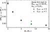 |
Fig. A.1. Amount of mass shed during Case BC RLOF for model B13.5p6.31 (green circle) re-calculated with different companion masses (black circles) and/or accretion efficiency of unity (gray diamonds). |
Our choice of qi = 0.5 means that in the vast majority of cases the accretor will be more massive than what we simulated, as lower qi tend to undergo unstable RLOF before producing a HeS (see Sect. 7.2.2). We can therefore expect that in the stable mass transferring channel, ΔMRLOF−BC will be similar to the values we estimated. We expect models with significantly less massive companions, like a NS, to have a higher ΔMRLOF−BC, in the order of ∼ 0.15 M⊙ from our expectation.
With regards to the mass-transfer rate before core collapse, we similarly observe small variations compared to the original run when changing the secondary's mass (see Fig. A.2.). The peak of the mass transfer rate happens earlier on for more extreme mass ratios (shifting by at most 500 yr) reaching values at most ≲10% higher. The shift of the peak at earlier times result in a more significant drop in the mass transfer rate in the last 100 yr before CC, by as much as a factor 2, which would decrease the probability of interaction-power dominating in the light curve of the exploding SN with a constantly expanding CSM (see Sect. 5.4). The opposite is instead true for higher-mass companions.
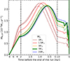 |
Fig. A.2. Mass transfer rate before the end of the run for model B13.5p6.31 (green, thick line) with different secondary masses (see legend). For solid lines indicate the models where mass transfer is assumed inefficient, while the dashed ones assume an accretion efficiency of unity. |
We focus on the effect of a higher mass transfer efficiency Case BC RLOF. We reran model B13.5p6.31 two times, with a companion M2 of 1 M⊙ and 7 M⊙ (i.e., that of the original model) and a mass transfer efficiency of 1. As the accretion of pure He on an MS star has proven difficult, we resorted to model this phase by setting the secondary star to a point mass. The amount of mass transferred is increased by a negligible amount (see Fig. A.2.), but this comes at the cost of no CSM being formed around the system at CC, therefore hindering the possibility of interaction features appearing in the SN. If accretion were to be efficient, the secondary star would inevitably show significant He- and N- enrichment on the surface (e.g., Richards et al. 2024) which will be more prominent for less massive companions.
Appendix B: A better parameter for calibrating the outcome of Case BC-RLOF
As we have shown in Sect. 4.2.2 (see Fig. 8), the amount of mass lost during Case BC ΔMRLOF−BC qualitatively scales with the time between the onset of RLOF and CC. As such, for a given binary-stripped HeS model, we can derive ΔMRLOF−BC by estimating when a single HeS model of the same mass at core He depletion MHe−dep reaches the donor's Roche lobe radius RRL, 1 (see Fig. 8). In this section we show that replacing MHe−dep with the maximum mass of the convective He-burning core  yields a more reliable estimate of ΔMRLOF−BC.
Since the single- and binary-stripped HeS models are known to have qualitative differences in their internal structures that affect radius evolution (e.g., Laplace et al. 2020), it is reasonable to assume that a single- and binary-stripped HeS with the same MHe−dep may not actually share the same radius evolution.
To identify such differences, we study the radius evolution of models B12.3p251, He2.86, and He2.99 (Fig. B.1.), which have similar MHe−dep (respectively 2.90, 2.86 and 2.99 M⊙; see Tables 1 and 2) in the range where we expect the sharpest difference in radii, especially at later times (see Figs. 2, 8). Although we expect that the radius evolution of model B12.3p251 should be an intermediate case between that of He2.86 and He2.99, instead we find that it is almost identical to that of model He2.86 (see Fig. B.1.) with which it also shares a very similar final CO-core mass (MCO, end = 1.62 M⊙). Since the mass of the core determines the luminosity and the remaining lifetime of the model, it will ultimately also determine the radius evolution. To investigate why model B12.3p251 does not exhibit an intermediate value for MCO, end between that obtained in model He2.86 and He2.99, we explore the evolution of each model during core He burning.
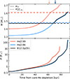 |
Fig. B.1. Mass of the CO core (top) and radius (bottom) as a function of time, for two single HeS models (He2.97 and He2.83, in red and blue respectively) and one binary-stripped HeS model (B12.3p251 in black). In the top panel, |

In He2.86 and He2.99, the total mass, initially 3.55 M⊙ and 3.76 M⊙ respectively, decreases steadily over time as winds erode the exposed He-rich layers. In B12.3p251, which retains a thin H-rich envelope, the mass of the He core is only 2.72 M⊙ at core He-ignition and grows to 3.35 M⊙ via H-shell burning before winds remove the H-rich envelope, reducing its mass (refer to Fig. 4 for a similar evolution). Thus, B12.3p251's He-core mass is initially smaller than He2.86 and He2.99 but later achieves an intermediate mass due to H-shell burning and winds. This impacts the He-burning core's luminosity and the extent of the convective region. In B12.3p251, the maximum mass reached by this region ( ) is 1.47 M⊙, smaller than He2.99's 1.61 M⊙ but again almost identical to He2.86's 1.48 M⊙.
At the moment of core He-depletion, a sharp decrease in He abundance occurs below the mass coordinate  , which therefore determines the region below which we expect to find the CO core. In the models, the mass of the CO core (MCO) is defined as the outermost mass coordinate with XHe<0.01, and it may not initially coincide with the location of the sharp drop in He abundance at
  (see Fig. B.1.), due to the leftover unburnt He. The He-shell burning that follows consumes the remaining He below
  , increasing MCO until it coincides with
  , typically by the start of core C-burning. Although MCO will continue growing afterward, it is evident that its value is intimately connected with
  .
.
In summary, the radius evolution for a binary-stripped HeS model can be accurately predicted by single HeS models with an identical  , rather than those with the same MHe−dep. Re-drawing Fig. 8 using
  in place of MHe−dep results in Fig. B.2., which now shows a better agreement between the trends for ΔMRLOF−BC and the radius evolution of single HeS models. These findings, along with the robustness of our estimates when varying the companion mass (see Appendix A), show the general predictive power of our method.

Appendix C: Interaction-powered luminosity
We assumed that the mass unaccreted during Case BC RLOF is ejected from the system and that it moves at a constant velocity vCSM. At t = 0, the SN explosion will expel a fast moving shell (i.e., the ejecta) with initial mass Mej and initial (bulk) velocity vej, which will gradually sweep the CSM as it travels through it. We followed the evolution of the portion of the fast-moving shell that interacts with the CSM. We refer to it as the cold dense shell (CDS, Chugai et al. 2004), which has an initial mass M(0) = Mej sin θ (depending on the opening angle of the CSM; see Sect. 5.3), and velocity v(0) = vej. We assumed that the CDS collides inelastically with the CSM, thus conserving momentum while losing kinetic energy which we assume is completely converted into radiation. We neglect any effect from photon-diffusion processes, and we only focus on the rate of energy loss from the CDS. Under this assumption, the amount of kinetic energy that is converted into radiation as the CDS sweeps through a small shell of mass dm is equal to
 (C.1)
(C.1)
Performing a series expansion for dm, under the assumption that at any given time interval dt we have dm≪M, results in
 (C.2)
(C.2)
which, if divided by the time interval, gives the interaction luminosity
 (C.3)
(C.3)
We can write a differential equation for the CDS's velocity v per conservation of momentum as
 (C.4)
(C.4)
The CDS's mass M will also increase over time, as the CDS gradually sweeps material from the CSM:
 (C.5)
(C.5)
Once  is known, Eq. C.4 and C.5 form a complete set of differential equations, once we include the initial conditions M(0) and v(0). Solving for M(t) and v(t), then Linter(t) can be evaluated using Eq. C.3. We note that the information on the geometry of the CSM is found inside dm and the initial condition on the CDS's mass.
Next, we describe the mass-element of the CSM, assuming this was either constantly expanding following mass loss from the inner binary or a CBD. For each case, we derive Linter.
C.1. Free-moving circumstellar material
If we assume that the CSM is polluted following mass-loss, with the material moving away from the system, we can use the mass-loss history of the system to infer the swept up mass dm per unit time dt.
To know the time at which the material dm was ejected before CC (tRLOF), one needs to solve the following integral equation, where the moment of CC is set to zero:
 (C.6)
(C.6)
As we have no constraint on vCSM, we assumed it constant for simplicity. With this, we can take the derivative of the previous equation by t to obtain the following differential equation:
 (C.7)
(C.7)
where a physical solution exists as long as v(t)>vCSM. This provides a scaling factor between the mass-loss rate from the system  and the amount of mass swept by the CDS as it travels through the CSM per unit time:
 (C.8)
(C.8)
where we retrieve ṀROLF from the model by looking up the mass-loss rate at a time tRLOF prior to CC by solving Eq. (C.7). Substituting this back into Eq. (C.3) yields
 (C.9)
(C.9)
For the generic solution, Eq. (C.9) needs to be coupled with Eq. (C.7), and the differential equations for the velocity and mass of the CDS (Eq. (C.4) and (C.5)), which are given by
 (C.10)
and we have to add the initial condition for the differential equation Eq. (C.7), that is, tRLOF(0) = 0.
C.2. Circumstellar material bounded in a circumbinary disk
We can assume that MCSM is bounded within a CBD (or, more precisely, a torus) of internal radius Rin, outer radius Rout and opening angle θ. We assume that the material inside the CBD has no bulk movement, such that vCSM = 0. We write the mass-element as follows:
 (C.11)
We worked under the assumption that  , with ρ0 as the characteristic density at a distance Rin, which is equal to
![Mathematical equation: $$ \rho _0= \begin {cases}{M_{\mathrm {CSM}}}\left [\frac {4\pi } {3+s} R_{\mathrm {in}} ^{-s} \left (R_{\mathrm {out}} ^{3+s}- R_{\mathrm {in}} ^{3+s}\right )\sin \theta \right ]^{-1} & s \neq -3 \\ {M_{\mathrm {CSM}}}\left [4\pi R_{\mathrm {in}} ^3\left (\ln \frac {{R_{\mathrm {out}}}}{{R_{\mathrm {in}}}}\right )\sin \theta \right ]^{-1} & s = -3 \\ \end {cases}. $$](/articles/aa/full_html/2025/04/aa53426-24/aa53426-24-eq55.gif) (C.12)
(C.12)
We defined the following quantity,
 (C.13)
which has the dimensions of a distance to the power of 3+s. We thus obtained the following form for the mass-element:
 (C.14)
We now have all the information necessary to rebuild the differential equations Eqs. C.4-C.5, by writing  , which are
 (C.15)
And finally, combining Eqs. C.3 and C.15 yields
 (C.16)
We note that because of the assumption that the disk is stationary, the equation for conservation of momentum simplifies to
 (C.17)
making one of the equations in Eq. (C.15) redundant. We use Eq. (C.17) to get rid of M(t) in the equations. We therefore only need to solve the equation of motion of the CDS, which is a second-order non-linear differential equation:
 (C.18)
where  and
and  . It is possible to obtain the generic (albeit implicit) solution for the case s≠−3, −4 which is given by
 (C.19)
where c1 and c2 can be determined using the initial conditions at  which are r(t0) = Rin and v(t0) = vej. We can therefore write the analytical expressions for r(t) and v(t) as
![Mathematical equation: $$ \left\{ \begin {array}{rl}r(t)-{v_{\mathrm {ej}}}t &= \frac {{M_{\mathrm {CSM}}}}{{M_{\mathrm {ej}}}\sin \theta }\left [\frac { R_{\mathrm {in}} ^ {s+3}(r(t)-{R_{\mathrm {in}}})}{ R_{\mathrm {out}} ^{3+s}- R_{\mathrm {in}} ^ {3+s}}-\frac {1}{4+s}\frac {r(t)^ {4+s}- R_{\mathrm {in}} ^{4+s}}{ R_{\mathrm {out}} ^{3+s}- R_{\mathrm {in}} ^ {3+s}}\right ] \\ v(t) &= {v_{\mathrm {ej}}}\left (1+\frac {{M_{\mathrm {CSM}}}}{{M_{\mathrm {ej}}}\sin \theta }\frac {r(t)^{3+s}- R_{\mathrm {in}} ^{3+s}}{ R_{\mathrm {out}} ^{3+s}- R_{\mathrm {in}} ^{3+s}}\right )^{-1} \end {array}\right .. $$](/articles/aa/full_html/2025/04/aa53426-24/aa53426-24-eq67.gif) (C.20)
(C.20)
All Tables
All Figures
|
Fig. 1. Evolution of the radius of single HeS models as a function of time during and after core carbon burning, with t = 0 set at core carbon depletion. The square markers indicate core carbon ignition, circles indicate the time when the first carbon shell develops, and stars mark the end of the calculation. For the lowest mass model, no endpoint is shown (see Sect. 3.1). |
| In the text | |
|
Fig. 2. Mass-radius diagram for single HeS models (showing the stellar radius, lines) and binary-stripped HeS models (showing the Roche lobe radius, symbols) as a function of the mass at core He-depletion MHe−dep. For single HeS models, the radius at a time t before the end of the run ( |
| In the text | |
|
Fig. 3. Plot of the log Pi−qi diagram for the binary grid of models from Jin et al. (in prep.), with M1, i = 12.6 M⊙. Each pixel represents one detailed binary evolution model. The color coding represents the mass of the primary star at core helium depletion. The solid lines cover the models where the radius of a single HeS of the same mass (see Fig. 2) matches their Roche lobe radius at core He depletion. White pixels are models that terminated before core-carbon ignition (see Sect. 2.4). The dotted patches correspond to the models which exhibited Case BC RLOF in the binary grid. The star marker in the top-left corner corresponds to the lowest-period model shown in Ercolino et al. (2024). |
| In the text | |
|
Fig. 4. Time evolution of the primary star in model M1, i = 13.5 M⊙, qi = 0.50, and Pi = 6.3 d from the onset of Case B RLOF (left), during core He burning (center), and until the end of the run (right). Top: Kippenhahn diagram. The outermost boundaries are colored corresponding to the most abundant element just below (see legend on the right), and the colored patches are based on the dominating mixing mechanism (see legend on the left). A dashed red line shows the maximum extent of the convective H-burning core during the MS. Bottom: Mass transfer rate (solid) and wind mass loss rate from the primary (dashed). |
| In the text | |
|
Fig. 5. Zoom-in of the Kippenhahn diagram close to the edge of the CO core where the Ne-burning shell ignites at a mass coordinate of 1.54 M⊙ and develops a convective region just above it that then merges with the He-burning shell after about 10 d. The solid lines, and patch colors are the same as in Fig. 4. The dashed lines correspond to the radius (black, dashed), the Roche lobe radius (red, dashed) and the volume-equivalent radius of the outer Lagrangian point (red, dotted). |
| In the text | |
|
Fig. 6. Spectroscopic HR-diagram of the binary-stripped models explored in this work. The models are color-coded by the mass at core He-depletion MHe−dep (see Fig. 3). Each track is plotted from the end of core He-burning until the onset of Case BC RLOF (filled circle). For those that do not undergo RLOF, the plot is shown until the point found at 20 yr before the end of the run (empty circle). The track of model B13.5p6.3 is highlighted in black and shown from ZAMS. The He-stars in the Small and Large Magellanic Clouds analyzed by and Götberg et al. (2023) are also shown (black squares), and numbered as in Drout et al. (2023). |
| In the text | |
|
Fig. 7. Mass loss as a function of time prior to the end of the run for the set of models with M1, i = 12.6 M⊙ with different initial orbital periods (marked by different colors). The three different panels highlight different timescales. |
| In the text | |
|
Fig. 8. Maps showing the ΔMRLOF−BC (top) and the amount lost after ṀROLF exceeds 10−4 M⊙ yr−1 (i.e., |
| In the text | |
|
Fig. 9. Scatter plot showing the compactness parameter ξm=(m/ M⊙)/(R(m)/1000 km) for m = 1.75 M⊙ (triangle marker) and 2.5 M⊙ (circle marker) as a function of the final CO core. The results of both the single (red) and binary-stripped HeS models (blue) are shown. The compactness is evaluated at core O-depletion for all models (empty markers), including at CC for those that reached it (gold fill). Models with Mend<2.5 M⊙ are shown with lighter colors. |
| In the text | |
|
Fig. 10. Properties of the primaries as a function of the final CO-core mass of the primary star. The markers are colored as a function of MHe−dep, as in Fig. 3. Top: Amount of mass ejected during Case BC RLOF. The empty markers represent the total mass lost via mass transfer, while the filled markers represent the mass shed during mass transfer after ṀROLF > 10−4 M⊙ yr−1 for the first time. Bottom: Amount of helium (circles) and metals (error bars) found in the ejecta. The uncertainty in the metal content derives from assuming Mns to be within 0.15 M⊙ of the fiducial value (horizontal marker). |
| In the text | |
|
Fig. 11. Circumstellar material in our models at the time of the SN, according to various estimates, versus the SN ejecta mass. The CSM mass given by ΔMRLOF−BC (white, with black outline) and |
| In the text | |
|
Fig. 12. Bar chart of the spatial distribution of material from the SN progenitor models 1 yr prior to the end of the run for the models run in this work. Color bars highlight the envelope (blue filled bar) and the regions where the CSM would be found (hatched bars) if it were distributed along a CBD (green) or if it were expanding isotropically, at a constant speed of 10 km s−1 (gray). In the latter case, the minimum radius is set as the point where the cumulative mass of the CSM from the progenitor star reaches 0.001 M⊙, and increases in contrast when it reaches 0.01, 0.1 and 0.5 M⊙. The Roche lobe radius of the progenitor star is shown (blue hatched-line) as well as the volume-equivalent radius of the outer Lagrangian point (red hatched-line). Finally the companion's location is also shown (orange marker) alongside its Roche lobe (vertical orange hatched-line). The models are grouped by different initial masses (indicated in the bottom of each box). |
| In the text | |
|
Fig. 13. Interaction-powered light curves for model B12.3p25.1 assuming a constantly expanding CSM (left panel) and a CBD-like CSM (right panel). A comparison of the two approaches with different explosion energies is shown in the center panel. In each panel, two observations are shown, namely, the Type Ibn SN OGLE-2012-SN-006 (Pastorello et al. 2015a, light-blue scatter) and the Type Icn SN 2019jc (Pellegrino et al. 2022b, orange scatter) as well as the template light curves for Type Ibc SNe (Nicholl et al. 2015, in violet, where the peak is located at the same time as in the light curve of model he4 from Dessart et al. 2020) and Type Ibn SNe (Hosseinzadeh et al. 2017, in blue, where the peak is arbitrarily placed at 10 d). Left: The CSM is assumed to constantly be expanding at vCSM = 10 km s−1, with different opening angles (with different colors) and with Ekin, ej = 6×1050 erg. For θ = 90°, models with vCSM of 5 km s−1 (dotted line) and 20 km s−1 (dashed line) are also shown. Center: Interaction power from the CBD-like CSM (solid, with Rin = 1013 cm, Rout = 1015 cm, and s=−1) and a constantly expanding CSM (dashed, with vCSM = 10 km s−1) are shown with different Ekin, ej (different colors), assuming an opening angle θ = 10°. Right: The CSM is assumed to be CBD-like, with Rin = 1013 cm, Rout = 1015 cm, s=−1 and different opening angles (different colors). For θ = 5°, the cases with s = 0 (dashed) and s=−2 (dotted) are also shown. |
| In the text | |
|
Fig. 14. Comparison between model data and parameters inferred from observed Type Ibn SNe (blue-scale colored markers). The different markers are associated with different SNe, and different colors for the same SN highlight different references. Estimates inferred from the models of WF22 are also included and are shown as in Fig. 11. Top left: Scatter plot showing the amount of mass of the CSM against the ejecta mass in the models as in Fig. 11. As the values of MCSM from the models is an upper limit, a light-gray region is added where models can still be expected. Right: Scatter plot showing the extent of the CSM against its mass. The position of CBD-like CSM from our models is shown with a gray line for MCSM=ΔMRLOF−BC. The region where CBDs from the models in the binary grid are expected to be found is shown with a vertically hatched region. The radii of our theoretical model are also shown (cross scatter). A gray patch is drawn where to expect the CSM if it were to move constantly at a speed of 10 km s−1. Bottom left: Scatter plot showing the energy released by interaction (Eq. (2)) as a function of CSM mass for the models in this work and WF22 assuming Ekin, ej = 6×1050 erg (shown with a black horizontal line) and the total light-curve energy of the observed SNe. The shaded regions represent the typical Erad of Type Ibc (light-red, Nicholl et al. 2015) and Type Ibn SNe (light-blue, Hosseinzadeh et al. 2017). The values expected from our models and those in the binary grid are summarized in gray regions, which also show the expected Erad if MCSM is lower than the values inferred. Each gray region assumes that the CSM is distributed spherically (solid line, light-hatch), along a CBD with θ = 15° (dashed line, dense hatch) and 5° (dotted line, gray fill) of the orbital plane (see Eq. (4)). References: SN2006jc: (1) Mattila et al. (2008), Pastorello et al. (2007); (2) Tominaga et al. (2008), Pastorello et al. (2007); (3) Chugai (2009), Pastorello et al. (2007); (4) Dessart et al. (2022), Pastorello et al. (2007); SN2010al: (5) Chugai (2022); SN2011hw: (6) Dessart et al. (2022), Pastorello et al. (2015b); LSQ13ddu: (7) Pellegrino et al. (2022a), Clark et al. (2020); (8) Clark et al. (2020), Brethauer et al. (2022); ASASSN-15ms: (9) Vallely et al. (2018); iPTF15ul: (10) Pellegrino et al. (2022a), Hosseinzadeh et al. (2017); SN2018bcc: (11) Dessart et al. (2022), Karamehmetoglu et al. (2021); (12) Karamehmetoglu et al. (2021); SN2018gjx: (13) Prentice et al. (2020); SN2019uo: (14) Pellegrino et al. 2022a; Gangopadhyay et al. 2020; (15) Gangopadhyay et al. (2020); SN2019deh: (16) Pellegrino et al. (2022a); SN2019kbj: (17) Ben-Ami et al. (2023); SN2019wep: (18) Pellegrino et al. (2022a), Gangopadhyay et al. (2022); SN2020bqj: (19) Kool et al. (2021); SN2020nxt: (20) Wang et al. (2024); SN2021jpk: (21) Pellegrino et al. (2022a); SN2022ablq: (22) Pellegrino et al. (2024); SN2023fyq: (23) Dong et al. (2024); SN2023tsz: (24) Warwick et al. (2025). |
| In the text | |
|
Fig. 15. Same as Fig. 14 but for Type Icn SNe and the Type Ic-CSM SN 2010mb. References: SN2010mb: (1) Ben-Ami et al. (2014), Brethauer et al. (2022); SN2019jc: (2) Pellegrino et al. (2022b); SN2019hgp: (3) Gal-Yam et al. (2022); (4) Pellegrino et al. (2022b), Gal-Yam et al. (2022); SN2021csp: (5) Pellegrino et al. (2022b), Perley et al. (2022); SN2022ann: (6) Davis et al. (2023); SN2023emq: (7) Pursiainen et al. (2023). |
| In the text | |
|
Fig. 16. Plot of the log Pi−qi diagram for the Case B binary models in the binary grid from Jin et al. (in prep.) with M1, i = 12.6 M⊙. The color coding is based on the amount of mass expected to be shed during Case BC RLOF. The hatching indicates models that are flagged as having undergone unstable Case B RLOF according to the criterion from Marchant (2017) (single hatch), Pauli (2020) (cross hatch), and Pavlovskii & Ivanova (2015) (circle hatches). |
| In the text | |
|
Fig. 17. Same Kippenhahn plot shown in Fig. 5 for model B13.5p6.31 (Sect. 4.1) that was reran from core O-depletion without any overshooting. The zero point in the x-axis is set to the onset of convective core Si-burning. The black arrow shows the moment when core Si-burning ends. |
| In the text | |
|
Fig. A.1. Amount of mass shed during Case BC RLOF for model B13.5p6.31 (green circle) re-calculated with different companion masses (black circles) and/or accretion efficiency of unity (gray diamonds). |
| In the text | |
|
Fig. A.2. Mass transfer rate before the end of the run for model B13.5p6.31 (green, thick line) with different secondary masses (see legend). For solid lines indicate the models where mass transfer is assumed inefficient, while the dashed ones assume an accretion efficiency of unity. |
| In the text | |
|
Fig. B.1. Mass of the CO core (top) and radius (bottom) as a function of time, for two single HeS models (He2.97 and He2.83, in red and blue respectively) and one binary-stripped HeS model (B12.3p251 in black). In the top panel, |
| In the text | |
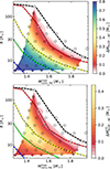 |
Fig. B.2. Same maps shown in Fig. 8, where the x-axis is |
| In the text | |
Current usage metrics show cumulative count of Article Views (full-text article views including HTML views, PDF and ePub downloads, according to the available data) and Abstracts Views on Vision4Press platform.
Data correspond to usage on the plateform after 2015. The current usage metrics is available 48-96 hours after online publication and is updated daily on week days.
Initial download of the metrics may take a while.