| Issue |
A&A
Volume 619, November 2018
|
|
|---|---|---|
| Article Number | A131 | |
| Number of page(s) | 22 | |
| Section | Extragalactic astronomy | |
| DOI | https://doi.org/10.1051/0004-6361/201833916 | |
| Published online | 15 November 2018 | |
Super star cluster feedback driving ionization, shocks and outflows in the halo of the nearby starburst ESO 338-IG04⋆
Department of Astronomy, Stockholm University, Oscar Klein Centre, AlbaNova University Centre, 106 91 Stockholm, Sweden
e-mail: This email address is being protected from spambots. You need JavaScript enabled to view it.
Received:
20
July
2018
Accepted:
7
September
2018
Abstract
Context. Stellar feedback strongly affects the interstellar medium (ISM) of galaxies. Stellar feedback in the first galaxies likely plays a major role in enabling the escape of LyC photons, which contribute to the re-ionization of the Universe. Nearby starburst galaxies serve as local analogues allowing for a spatially resolved assessment of the feedback processes in these galaxies.
Aims.We aim to characterize the feedback effects from the star clusters in the local high-redshift analogue ESO 338-IG04 on the ISM and compare the results with the properties of the most massive clusters.
Methods. We used high quality VLT/MUSE optical integral field data to derive the physical properties of the ISM such as ionization, density, shocks, and performed new fitting of the spectral energy distributions of the brightest clusters in ESO 338-IG04 from HST imaging.
Results.We find that ESO 338-IG04 has a large ionized halo which we detect to a distance of 9 kpc. We identify four Wolf-Rayet (WR) clusters based on the blue and red WR bump. We follow previously identified ionization cones and find that the ionization of the halo increases with distance. Analysis of the galaxy kinematics shows two complex outflows driven by the numerous young clusters in the galaxy. We find a ring of shocked emission traced by an enhanced [O I]/Hα ratio surrounding the starburst and at the end of the outflow. Finally we detect nitrogen enriched gas associated with the outflow, likely caused by the WR stars in the massive star clusters.
Conclusions. Photoionization dominates the central starburst and sets the ionization structure of the entire halo, resulting in a density bounded halo, facilitating the escape of LyC photons. Outside the central starburst, shocks triggered by an expanding super bubble become important. The shocks at the end of the outflow suggest interaction between the hot outflowing material and the more quiescent halo gas.
Key words: galaxies: starburst / galaxies: halos / galaxies: kinematics and dynamics / galaxies: individual: ESO 338-IG04 / techniques: imaging spectroscopy
Based on observations made with ESO Telescopes at the La Silla Paranal Observatory under programme 60.A-9314 (Science verification) and on public data released from the MUSE commissioning observations at the VLT Yepun (UT4) telescope under Programme ID 60.A-9100(C).
© ESO 2018
1. Introduction
Young massive stars have a strong impact on their surroundings. They destroy the molecular clouds they are born in and ionize the surrounding interstellar medium (ISM) via copious amount of Lyman continuum (LyC) photons. Stellar winds and, at a later stage supernova explosions inject large amounts of mechanical energy in the ISM, driving shocks and large scale outflows. Stellar feedback has strong effects on the evolution of the galaxies where the massive stars are located in. Feedback can trigger new sites of star formation (e.g. Adamo et al. 2012), or even suppress star formation by emptying large cavities around massive star clusters (e.g. Östlin et al. 2007; Pasquali et al. 2011).
At low-metallicity especially, the effect of the stellar feedback on the ISM of the galaxy is not well understood. A detailed understanding of stellar feedback in these environments and how it facilitates the escape of LyC radiation is particularly relevant as the leakage of the LyC from starburst galaxies is one of the candidates for the re-ionization of the universe (e.g. Robertson et al. 2015; Bouwens et al. 2015; Trebitsch et al. 2017). However, at high redshift these galaxies are hard to detect, let alone study in detail. Therefore studies of local galaxies with similar properties as the high-redshift star forming galaxies provide vital information in understanding how the feedback acts on the ISM and facilitates possible LyC leakage.
Blue compact (dwarf) galaxies (BCGs) are typically considered to be local analogues of high redshift star forming galaxies. They are compact, characterized by a highly elevated star formation rate and low metallicity (Searle & Sargent 1972; Izotov & Thuan 1999). These galaxies typically have an ongoing starburst super imposed on a much older stellar population (Loose & Thuan 1986; Kunth et al. 1988; Papaderos et al. 1996a,b; Kunth & Östlin 2000; Bergvall & Östlin 2002; Gil de Paz et al. 2003). Their optical spectra are dominated by emission lines allowing a detailed characterization of the ISM properties and kinematics. Kinematical studies of BCGs reveal irregular velocity fields suggestive of their starburst being triggered by mergers involving dwarf galaxies or in-falling massive gas clouds (Östlin et al. 2001). BCGs are hosts of rich population of young stellar clusters (e.g. Meurer et al. 1995; Thuan et al. 1997; Östlin et al. 1999, 2003; Adamo et al. 2010a,b, 2011; Calzetti et al. 2015).
During the evolution of a star cluster different processes are responsible for the energy output that modify the ISM. According to stellar population models star clusters younger than ∼4 Myr (for metallicity Z = 0.004) emit the most amount of hydrogen and helium ionizing photons as even the most massive stars have not yet exploded as supernova (Leitherer et al. 1999). In this phase, ionization and radiation pressure are important mechanisms of feedback (Krumholz et al. 2014). After 3 Myr massive stars evolve into Wolf-Rayet (WR) stars. Their surface temperatures can reach values up to 100 000 K (Smith et al. 2002; Crowther 2007) and they emit large amounts of very hard photons, giving rise to the ionization of He+. At low metallicity (12 + log O/H < 8), however, evidence is found for a decreased importance of WR stars and that O stars could be the main source of He+ ionizing photons (Kunth & Schild 1986; Guseva et al. 2000; Brinchmann et al. 2008).
The strong stellar winds of massive stars are responsible for the output of mechanical energy in the ISM during the first 4 Myr of the cluster lifetime. Only after 4 Myr, when the first supernovae explode, mechanical energy is mainly produced by the supernovae. Until clusters reach an age of 40 Myr, their mechanical energy output (by stellar wind and later by supernovae) remains roughly constant (Leitherer et al. 1999). The mechanical energy of the stellar winds and supernovae heats up the surrounding ISM and creates a large, so called super-bubble, filled with hot, X-ray emitting gas (Weaver et al. 1977). In the theoretical picture of the formation of galactic winds (Chevalier & Clegg 1985; Strickland & Heckman 2009; Heckman & Thompson 2017), super-bubbles are the first stage in the creation of a galactic scale outflow. In the super bubble the reservoir of hot gas thermalized by the supernova explosions is built up. While expanding, the edge of the bubble becomes gravitationally unstable and breaks. This allows the hot gas to escape and form an outflow (the so-called blow-out phase). In a inhomogeneous medium, the outflowing material follows the path of least resistance and escapes via the low-density channels already present in the gas, created by for example previous generations of clusters (Cooper et al. 2008). The Hα emission is originating from the warm gas entrained by the outflow and the inner walls of the outflow cones (e.g. Westmoquette et al. 2009), as well as from radiatively cooling hot gas (Thompson et al. 2016).
In this paper we focus on one of the closest luminous BCG and high redshift analogue ESO 338-IG04 (hereafter shortened to ESO 338, α = 19h27m58.2s, δ = −41°34′32″), also known as Tololo 1924-416, at a distance of 37.5 Mpc1 (Östlin et al. 1998) and a metallicity of 12% solar (Bergvall 1985). The galaxy is a compact galaxy, currently undergoing a vigorous starburst which started 40 Myr ago and created a large young stellar cluster (YSC) population (Östlin et al. 1998, 2003; Adamo et al. 2011). The most massive young stellar cluster in this galaxy (cluster 23) has a dynamical mass of ∼107 M⊙ and is the most luminous and massive young (age < 10 Myr) cluster detected in nearby galaxies. This cluster has evacuated a large bubble in the ISM (Östlin et al. 2007). ESO 338 has a total stellar mass of 4 × 10⁹ M⊙ and a star formation rate of 3.2 M⊙ yr−1 (Östlin et al. 2001). The galaxy is surrounded by a large halo of ionized (Östlin et al. 1999; Bik et al. 2015) and neutral gas (Cannon et al. 2004). ESO 338 has a companion galaxy, ESO 338-IG04B, connected via a tidal tail observed in H I (Cannon et al. 2004). Cannon et al. (2004) suggests that a strong gravitational interaction between the two galaxy has triggered a starburst in ESO 338-IG04. However, the projected distance is rather large (∼72 kpc), suggesting that the current starburst may not have been triggered by this interaction. Summarizing, the relative proximity and extreme properties make ESO 338 a good environment to study the effect of cluster feedback at low metallicity.
We present deep optical integral field spectroscopy obtained with the Multi-Unit Spectroscopic Explorer (MUSE) of this galaxy where we observe the ISM and the extended halo of the galaxy. This data will allow us to obtain spatially resolved information on physical properties of the ISM such as density, extinction, degree of ionization, abundance and kinematics. In Bik et al. (2015) the first results of the MUSE observations on ESO 338 were presented, where we identified two ionization cones as well as two galactic scale outflows. We found that the Lyα emission preferentially escapes in the direction of the galactic scale outflows. This paper presents even deeper data by combining two different MUSE datasets on ESO 338. This unique dataset from MUSE enables us for the first time to make a direct comparison between the properties of the ISM and the young stellar cluster population in ESO 338 as derived from HST.
In this paper we combine the cluster analysis and the analysis of the ISM of ESO 338 in order to analyse the effect clusters have on the ISM of ESO 338 in detail. In Sect. 2, the data are presented and the data reduction is described. Section 3 summarizes the properties of the stellar clusters and especially those of the clusters containing WR stars. In Sect. 4 we derive the physical conditions of the ionized gas based on the emission line maps. In Sect. 5 we analyse the halo in further detail, by deriving its mass, apply a two dimensional analysis of emission line ratios using the so called BPT diagram (Baldwin et al. 1981), as well as analyse the galactic scale outflow in detail. In Sect. 6 we discuss the properties of the halo in the context of other galaxies and speculate on the possibility of ESO 338 being a LyC leaking galaxies. The paper ends with a summary and conclusions (Sect. 7).
2. Observations and data reduction
In this paper we present and analyse two datasets obtained with the integral field spectrograph MUSE (Bacon et al. 2010), mounted on the VLT on Paranal, Chile. The first MUSE dataset was obtained during the first science verification run on 2014, June 25. The data were taken in non-AO mode with the extended wavelength setting, providing spectra between 4600 and 9300 Å over a 1□′ field of view with a 0.2″ pixel scale. The first results of this dataset have been published in Bik et al. (2015). The integrations were split over 2 observing blocks (OBs) with each four frames of 750 s rotated by 90° each to minimize the systematics.
The second dataset was obtained during the second commissioning run on 2014, July 30 and 2014, August 3, also in non-AO mode and with the extended wavelength setting. This data was spit over 2 OBs with 4 frames of 900 s in the first OB and 3 frames of 900 s in the second OB (Table 1). No separate sky frames were taken for the datasets.
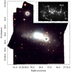 |
Fig. 1. Three-colour image made from VRI broad-band images reconstructed from the MUSE data-cube. The galaxy as well as several star clusters are apparent. The two brightest point sources in the image are foreground stars and are marked with a star symbol. The inset is the V-band image observed with HST (Östlin et al. 2009) with marked the four clusters with WR features in their spectra. |
Observing log.
2.1. Data reduction
Both datasets were reduced with the ESO pipeline version 1.2.0 (Weilbacher et al. 2012), resulting in an improved data cube, with significantly better sky subtraction than the data presented in Bik et al. (2015), processed with a much earlier version of the pipeline. For the science verification data set, slit 6 of IFU 10 is vignetted and contains very low flux due to data acquisition at low instrument temperature. The ESO provided trace tables for this slit were used to get a wavelength calibration. The slit has been removed from the science data. The dataset taken during commissioning does not have this problem.
2.2. Sky subtraction
As the Hα and [O III]5007 Å lines extend to the edge of the observed field of view, special care has been taken to properly remove the sky background. The edges of the fields, where the Hα and [O III]5007 Å are not present are too small, resulting in a low signal-to-noise ratio (S/N) sky spectrum. Applying this spectrum results in a bad correction of the emission lines, especially in the red part of the spectrum.
We therefore applied a different approach to remove the sky emission without affecting the nebular emission lines. This process was done in two steps. Firstly, a sky background was created with the pipeline using a skymodel_fraction = 0.2 in the scipost procedure. After inspection of the resulting sky spectrum, emission lines of Hα, Hβ [O III]5007 Å and 4959 Å are present. These were removed by interpolating below these lines in the SKY_CONTINUUM file. The SKY_CONTINUUM should contain only a smoothly varying continuum, as it is created after the sky lines have been subtracted. Any residuals in this spectrum are either sky line subtraction residuals or extended emission lines. None of the selected emission lines were contaminated by sky line residuals. The modified SKY_CONTINUUM file was then again inserted in the pipeline and scipost was run again with the modified sky as input, resulting in a much better removal of the sky lines. This approach has been also successfully applied in Herenz et al. (2017).
We then extracted line maps for the emission lines of scientific interest by numerically integrating under the line profile. The continuum underneath the line was estimated by averaging the continuum left and right of the emission line and subtracted. The corresponding noise frames were extracted from the error cube by quadratically summing the error over the wavelength range the line is integrated. On the line maps we checked for residual sky emission or absorption the following way: we applied a weighted Voronoi tessellation binning algorithm by Diehl & Statler (2006), which is a generalization of the Cappellari & Copin (2003) algorithm, with a S/N of 5 and a maximum cell size of 2500 pixels to detect the line emission and subtracted the emission with a S/N > 5 from the line map. The resulting map now only contains residual sky emission. We fitted a Gaussian function to the histogram of the sky values to calculate the centroid of the distribution. The centroid was then subtracted from the original map, making sure that the sky pixels have values centred around 0. The typical sky residuals found this way are below 1.5 × 10⁻²⁰ erg s−1 cm−2.
Finally, the data of the two datasets were combined into one final data cube. This data cube is about twice as deep in exposure time as the data presented in Bik et al. (2015). The final image quality is 0.9″ as measured on a reconstructed V-band image. Figure 1 shows a three-colour image of the VRI broad-band images extracted from the final data cube, showing the galaxy and the surrounding star clusters as well as some background galaxies. Two bright foreground stars are marked with a star sign.
3. Young stellar clusters
The galaxy ESO 338 hosts a large YSC population, formed during the current starburst. Östlin et al. (1998, 2003) carried out a detailed analysis of the stellar population based on NUV, UBVI HST imaging. They found that the present starburst has been active since 40 Myr. Adamo et al. (2011) showed that the cluster formation rate in ESO 338 has strongly increased since ∼20 Myr. They also showed that the amount of stellar mass forming in clusters with respect to the total stellar mass formed in ESO 338 is very high (50 ± 10%), making this galaxy an excellent show case in studying the feedback of YSCs on the ISM.
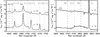 |
Fig. 2. Spectra of cluster 23 (top) and cluster 18 (bottom) highlighting the WR features in their spectra. The spectrum of cluster 23 is scaled down with a factor 2.8 to fit in the same scale. Left panel: spectral region around the He II 4686 Å line. The broad emission component is the signature of the presence of WR stars, the other WR lines (N III and C III) are not detected. The narrow component of He II is originating in the diffuse gas. Additionally, all the nebular emission lines are marked. Right panel: spectral region around the red WR bump. This emission bump is originated by C IV, tracing WC stars. Cluster 23 only shows a faint bump, while cluster 18 shows a very strong feature. |
Östlin et al. (2009) presented additional Hα imaging as well as far-UV data, allowing a better constraint on the ages of the very young clusters, covering the energy distribution between ∼1400 Å and 9500Å, including narrow band Hα. Following the procedure outlined in Adamo et al. (2010a) we constructed spectral energy distributions (SEDs) of the clusters. A cluster catalogue is created by detecting the clusters in the F550M and F814W filters independently using SExtractor (Bertin & Arnouts 1996). We created the final cluster catalogue by merging the catalogues of the two filters and requiring a detection in both the F550M and F814W images. Aperture photometry was performed to all bands with the cluster catalogue as input with fixed aperture size of 0.125″ in all the bands. The inner radius of the sky annulus was set at 0.15″ with a width of 0.05″.
3.1. SED fitting
The bright clusters discussed in this paper have a high S/N detection in all six bands (UV (F140LP), U (F336W), B (F439W), V (F550M), Hα (FR656N), I (F814W) and their SEDs were fitted to the latest version of the Yggdrasil models (Zackrisson et al. 2011) using χ2 minimization. These models take into account the contribution of both single stellar population models (Starburst99, Leitherer et al. 1999) with a Kroupa (2001) initial mass function (IMF) and gaseous continuum and emission lines produced with Cloudy (Ferland et al. 2013).
The models assume a stellar metallicity of Z = 0.004 and a density of the ionized gas of ne = 100 cm−3 (see for more details Adamo et al. 2017). The model fits are performed for three different covering fractions (0, 0.5 and 1.0). A covering fraction of unity means that all the LyC photons emitted by the cluster are absorbed by surrounding gas inside the photometry aperture, resulting in nebular emission. As shown in Adamo et al. (2010b) the strongest source of nebular contribution is the free-free emission. For the first 3–4 Myr, this can be as high as 50–60% of the flux in the broad-band filters, but strongly declines after 4 Myr.
The overall results of the fit are similar to the results presented in Östlin et al. (1998, 2003), showing that ESO 338 contains numerous YSCs with ages between 0 and 40 Myr, whose ionizing photons and mechanical energy strongly affect the surrounding ISM. We will discuss the stellar population in detail in a forthcoming study and for this paper we only look at some of the most massive young stellar clusters where we find evidence for WR stars based on their MUSE spectra.
3.2. Wolf-Rayet clusters
The WR phase is a short phase in the life time of a massive star. In this evolutionary stage, the evolved massive stars expel their outer layers with a very strong stellar wind (Crowther 2007). As the inner regions of the stars become optically visible, their effective temperatures can be as high as 100 000 K (Smith et al. 2002). This hot temperature makes the WR stars important contributors to the emitted He+ ionizing photons. Additionally, due to their strong winds, they also contribute to the chemical enrichment of the galaxies ISM (e.g. Monreal-Ibero et al. 2012). However, at low metallicity the contribution of the WR stars in the ionizing budget becomes less important (Kunth & Schild 1986; Guseva et al. 2000) and O stars significantly contribute to the He+ ionizing budget (Brinchmann et al. 2008). Recent studies show that standard population synthesis models cannot account for the amount of observed He II emission (Kehrig et al. 2015, 2018). After excluding possible contributions of shocks and gas accretion, very massive stars, or very low metallicity stars need to be used to explain the observed He II emission.
Assuming a single burst of star formation, massive stellar clusters with ages between 3 and 5 Myr show spectral features originating from WR stars (e.g. Leitherer et al. 1999; Smith et al. 2002). The spectral features of WR stars in the optical consist of two broad emission features (Fig. 2). The “blue” WR bump consists of broad He II 4686 Å emission as well as fainter C III and N III emission, while the “red” WR bump is observed at 5808 Å and is caused by C IV emission (e.g. Schaerer et al. 1999; Smith et al. 2016).
In order to find the clusters with these WR features we constructed a pseudo narrow band image (width = 100 Å) covering the red WR bump and subtracted the underlying continuum by interpolating between the blue and the red side of the emission band. We used the same method to construct a pseudo-image of the broad He II emission. Here we selected the broad emission only and leave out the narrow He II emission as well as [Fe III] and [Ar III] with a width of 10 Å left and right of the narrow He II emission. The velocity differences of the ionized gas are relatively low (see Sect. 4.5), therefore there is no contamination expected from the [Fe III] and [Ar III] in the pseudo images. The narrow He II is originating in the diffuse gas and will be discussed in Sect. 4.4.
Clusters in ESO 338 with WR features.
We found four clusters with WR features in their spectrum; all four show the broad He II emission and three clusters show the red WR bump. These clusters show clear signs of the WR features and are rather isolated such that the emission can unambiguously be related to the cluster. Fainter clusters might well have WR features present, but they were not visible as strong signals in the narrow-band images, and also are more difficult to detect due to the lower spatial resolution of MUSE compared to HST. The clusters are identified on the HST V-band image in Fig. 1 using the IDs from the inner sample of Östlin et al. (1998). Clusters 18, 23 and the source coinciding with clusters 50 and 51 all show both the blue and the red WR features, while cluster 53 only shows the broad He II emission. Figure 2 shows the blue and red WR features of cluster 23 and 18 extracted with a circular aperture with a 2 pixel (0.4″) radius. This aperture is small enough that the continuum emission from the clusters could be isolated and is free from contamination of other bright clusters. We did not subtract any background as in the continuum that is negligible (they are very bright clusters) and it would only create over- or under-subtraction of the nebular lines as they are varying in intensity on small spatial scales. Both clusters show the broad He II emission feature at 4686 Å with super imposed a narrow component originating in the ionized H II region. Also other nebular emission line from [Ar III] and [Fe III] are identified. From the two other WR lines (N III and C III) we see a hint of N III emission in cluster 18.
Table 2 summarizes the properties of the clusters as derived from fitting the Yggdrasil models to the cluster SEDs. All four clusters are among the most massive in the galaxy with masses of ∼105 M⊙ or higher. The reason why only those clusters show detected WR features is that they have the highest S/N spectra. There will be many more lower-mass clusters containing WR stars, but their features will be fainter and harder to detect. Below we discuss the properties of each cluster:
Cluster 23 is the most massive cluster of ESO 338 with a photometric mass of 3.8 × 10⁶ M⊙. Östlin et al. (2007) derive a dynamical mass based on cross correlation of the spectrum with stellar templates and derived a dynamical mass of 1.3 × 10⁷ M⊙. The discrepancy between the photometric and dynamical mass can be explained by the presence of spectroscopic binaries (Portegies Zwart et al. 2010). From fitting the Balmer absorption lines, they also derived an age of  . This cluster is located inside a large bubble which is the results of evacuated gas due to the feedback of the stellar population inside cluster 23 (Östlin et al. 2009). Based on the expansion speed of [O III] and Hα an expansion age of the bubble of 3–4.5 Myr is derived (Östlin et al. 2007), suggesting that the cluster expelled its gas very early in its evolution (Bastian et al. 2014).
By modelling the feedback from stellar winds and supernova explosions Krause et al. (2016) modelled the shell expansion around cluster 23 and try to explain the size and velocity of the bubble. By assuming a star formation efficiency of 30%, the energy injected by stellar winds and supernovae is not enough to clear the gas out of the cluster and create a bubble of the size observed. A star formation efficiency as high as 80% is required to explain the rapid gas expulsion of cluster 23.
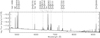 |
Fig. 3. Integrated MUSE spectrum centred on cluster 23 (α = 19h27m58.429s, δ = −41°34′30.74″) extracted with an aperture of 3″, covering the central regions of ESO 338. The emission lines used in this paper are labelled in the spectrum. We note that this spectrum contains one of areas where [O III] and Hα are saturated. |
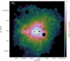 |
Fig. 4. Logarithmic scaled Hα emission line map of ESO 338 showing the spatial extend of the ionized halo. A Voronoi binning with minimum S/N of 5 and maximum bin size of 900 pixels (∼6□″) was applied. The Voronoi cells which have lower S/N than 5 are removed and plotted as black. Plotted in black contours are the contours of the I-band image reconstructed from the MUSE cube. Contour levels are 15, 50, 100, 400, 700 and 1000 × 10−20 erg s cm−2 Å−1. The lowest contour corresponds to an AB I-band magnitude of 25.2 mag. The saturated parts of the Hα image in the centre as well as the two bright foreground stars are masked out and appear as black. |
The age of the cluster as result of our SED fitting strongly depends on the choice of covering fraction. For cluster 23, a covering fraction of 0.0 was chosen, as the gas is blown out well beyond the photometry aperture of 0.125″. The derived age (4 Myr) and mass (3.8 × 10⁶ M⊙) (Table 2) are consistent with previous measurements as well as with the presence of WR features in the spectrum (Table 2). If we would, unrealistically, assume a much higher covering fraction, the low intensity of Hα close to the cluster would have resulted in a much older age; for a covering fraction of 1.0 the SED fitting produces an age of 15 Myr.
Cluster 18 is located in the south-eastern part of the galaxy and also has cleared out most of it’s gas content. It is located near a bow-shock like feature visible in Hα (Östlin et al. 2009). The ages and masses derived for this cluster assuming a covering fraction between 0 and 0.5 are 3–6 Myr and 3.6−4.0 × 10⁵ M⊙ respectively. Similar to cluster 23, in the case of a unrealistically covering fraction of 1.0, the derived age would be 15 Myr. This cluster has the strongest red WR bump of all four clusters, clearly identifying the presence of WC stars.
Clusters 50/51 were identified by Östlin et al. (1998) as two separate clusters. However, in our analysis of the HST data, only a single source has been identified. This cluster has strong Hα emission and has most likely not cleared its gas yet. Therefore we have chosen a covering fraction between 0.5 and 1.0. It is the lowest mass system in our sample with a mass of 0.8–1.3 × 10⁵ M⊙.
Cluster 53 shows a weak blue WR bump and no red bump, suggesting that not many WR are present. Also this cluster has likely not cleared it’s gas content yet as a lot of Hα emission is present on-source, favouring a high covering fraction.
4. Physical properties of the ionized gas
In this section we investigate the properties of the ionized gas in the halo of ESO 338. We derive physical properties like the extinction, density, and level of ionization using the recombination and collisionally excited lines present in the MUSE spectrum of ESO 338 (Fig. 3). Additionally, we discuss the kinematics of the halo based on the Hα emission line.
Figure 3 shows the MUSE spectrum integrated over a circular aperture with a radius of 3″, centred on the position of cluster 23 with the most important lines annotated. The Hα and the [O III] 5007 Å lines are the strongest lines in the data cube. Towards the three brightest regions in the galaxy these lines appear saturated in a large fraction of the individual exposures. All the other emission lines are significantly fainter and saturation is no issue. In the analysis of the emission lines where Hα and/or [O III] 5007 Å are included, we do not use the saturated parts of the data and they are clearly marked in the Hα line map (Fig. 4) and other figures where these lines are used.
Table 3 lists the emission lines used for each diagnostic. We applied Voronoi binning to all diagnostics in order to increase the S/N in the outer regions of the halo. The Voronoi pattern has been calculated on the faintest line (marked in boldface) and was then applied to the brighter line(s) used for the same diagnostic. For the diagnostics where line ratios are calculated we typically choose a higher S/N than for just emission lines maps.
4.1. Correction for stellar absorption
Two of the important emission lines used in the analysis of the ionized gas in ESO 338 are Hβ (4861 Å) and Hα (6563 Å). Inspection of the Hβ line profile shows absorption underneath the emission line in some locations of the galaxy. This is caused by a young and intermediate age underlying stellar population (González Delgado & Leitherer 1999; González Delgado et al. 1999). This absorption will also be present underneath Hα, but much harder to see due to the brightness of Hα and nearby [N II] lines. In order to measure the correct strength of the emission lines, this absorption needs to be corrected for. We corrected for the absorption lines by fitting simultaneously the emission and underlying absorption. In the regions of the galaxy where stellar continuum is present we fitted the emission with a Gaussian profile and the absorption with a Lorentzian profile, better reproducing the broad absorption winds of the Hβ absorption.
To determine where to estimate the continuum level, we smoothed the cube with a boxcar with a width of 5 × 5 pixels (1″2). Following González Delgado & Leitherer (1999), we measured the continuum near Hβ at ±30 Å away from the line centre with a width of 10 Å for each side. A linear fit between the two continuum apertures was performed and removed from the Hβ spectrum. From these background values a continuum image was constructed. We choose a flux level of 3.0 × 10⁻¹⁹ erg s−1 cm−1 Å−1 per pixel to determine whether a continuum is present or not.
For the regions where continuum is present both a fit with a single Gaussian emission and a fit with a Lorentzian absorption and Gaussian emission profile were made. The solution with two lines is only selected if the χ2 more than 10% better than that of the single line fit. The fit is performed on the smoothed data cube to increase the area of the galaxy where the absorption can be fitted. The correction on the emission line is calculated from the fit to the smoothed data and applied to the un-smoothed emission line flux. The regions in the cube without continuum do not need to be corrected and are therefore fitted with a single Gaussian tracing the emission line. Finally, we corrected Hα for the underlying absorption, adopting a ratio between the EW of Hα and Hβ of 0.65 as derived by Olofsson (1995) for a Z = 0.001, young (<15 Myr), stellar population. This value varies with age and IMF of the underlying stellar population. As the applied corrections are typically very small, this has negligible influence on the corrected Hα emission line flux. The applied corrections to the Hβ line-flux map range from less than 1% in the central 10″ of ESO 338, where the absorption cannot be detected due to the very strong emission to 60% towards some of the older clusters in the outskirts of the halo.
Diagnostics.
Figure 4 shows the absorption corrected emission line map of Hα. A Voronoi binning with a minimal S/N of five and a maximum area of 900 pixels was applied and result in a detection limit for Hα of 6.25 × 10⁻¹⁹ erg s−1 cm−2 □″, integrated over the line profile.
In Bik et al. (2015) the Hα line map already has been presented, showing the large halo which is surrounding ESO 338. However, with the inclusion of the commissioning dataset the depth of the dataset is twice as deep in exposure time and reveals the presence of ionized gas even further out to a distance of ∼8 kpc. Additionally, the halo is not smooth as a lot of spatial structure is visible in the emission map. Towards the south some filaments pointing outwards and to the north a more clumpy structure are present. Towards the northern edge the Hα emission seems to be even more extended than the observed frame.
4.2. Extinction
We used the ratio of the stellar absorption corrected Hα and Hβ to calculate a spatially resolved extinction map. As the metallicity of ESO 338 is low (Östlin et al. 2003; Bergvall 1985) and similar to the SMC, we applied the extinction law of Prevot et al. (1984) to determine the E(B – V) of each pixel. The extinction coefficients were taken from McCall (2004). We adopted an intrinsic value of the Hα over Hβ ratio of 2.86, assuming Case B, a density of 102 cm−3 and an electron temperature of 104 K (Osterbrock & Ferland 2006). We calculated the Voronoi tessellation pattern on the Hβ map to make sure that the individual cells have a minimum S/N of 30 over a maximum area of 900 pixels (6□″), aiming at an error of ∼0.04 mag in E(B – V). This pattern is applied to the Hα line map and the ratio map is made after that.
Figure 5 shows the resulting spatially resolved E(B – V) map. The E(B – V) map covers a smaller spatial extend than the Hα emission line map as the Hβ line is fainter and the minimum S/N for the Voronoi binning is reached at smaller radii. The E(B – V) map is corrected for a galactic foreground extinction of E(B – V)fg = 0.0742 ± 0.0011 mag (Schlafly & Finkbeiner 2011). The mean value for E(B – V) towards ESO 338 is 0.066 mag, with a standard deviation of 0.077 mag. The typical error per pixel on the E(B – V) is 0.03 mag, with smaller values in the centre where the Hα and Hβ flux are very high and higher values, up to 0.05 mag near the outskirts of the halo.
This map shows that ESO 338 has very low, or even no, extinction by dust. This is consistent with previous measurements of the extinction towards ESO 338 based on long-slit spectroscopy (e.g. Bergvall 1985; Rivera-Thorsen et al., in prep.) or SED modelling of the cluster population (Östlin et al. 1998, 2003).
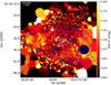 |
Fig. 5. E(B – V) map towards ESO 338 derived from the Hα/Hβ ratio. Both lines are corrected for underlying absorption of the stellar population. The extinction law of Prevot et al. (1984) is used and the plotted E(B – V) is corrected for the galactic foreground extinction. The blue contours are the contours of the I-band image reconstructed from the MUSE cube (identical to the black contours in Fig. 4). The saturated parts of the Hα image in the centre as well as the two bright foreground stars are masked out and appear as black. The high E(B – V) values at the outskirts are cells with relatively low S/N. The figure is zoomed in with respect of Fig. 4. |
We can see some spatial variation in the E(B – V) map. The highest values are reached to the eastern and western part of the galaxy. This is also where the Hβ absorption correction is the strongest. Lower values are reached extending away from the galaxy into the halo in northern and southern direction. This coincides with the two ionization cones identified in Bik et al. (2015) and the low E(B – V) is consistent with the high degree of ionization where dust is not expected to survive (see also Sect. 4.4). We also find an increase in the measured E(B – V) values towards the HII regions surrounding the massive clusters in the centre of the galaxy. The E(B – V) values become as high as 0.18 mag, compared to ∼0.05 mag in the surrounding gas. This indicates that there is still some dust present tracing the left-overs of the giant molecular clouds the clusters have formed in.
4.3. Electron density
In the MUSE spectral range we find several line ratios which can be used as a tracer for electron density or temperature. We can derive the electron density from the [S II] 6717 Å/6731 Å line ratio. Two sets of lines can be used to derive the temperature: [S III] lines and the [N II] line ratios. For the temperature, the detection of the faint auroral line ([N II] 5755 Å, or [S III] 6312 Å) is required. These lines can only be detected towards the bright central 10 × 15″ of the galaxy. The lines for the density ([S II] 6717 Å and 6731 Å), however, are much brighter and the density can be traced much further out. The spatially resolved maps of the temperature and density of the inner area of the galaxy will be part of a future study.
In this paper we derive the radial profile of the electron density in order to derive the total mass of the ionized halo (Sect. 5). To derive the electron density as far out in the halo as possible, we constructed a radial profile of both [S II] emission lines. The centre of the radial profile is the location of the brightest, central cluster, cluster 23 (the same positions as the extracted spectrum of Fig. 3). The bin width of the radial profile is chosen such that a minimum S/N of 30 is reached in the faintest [S II]6731 Å line up to a maximum bin width of 2″. The electron density is derived by adopting a temperature of 12 000 K (a typical value derived from both temperature traces in the central part of the halo) using getTemDen in pyneb.
Errors were calculating using a Monte Carlo approach. Based on the derived errors on the line fluxes, the line ratio is calculated 1000 times by randomly drawing from a Gaussian distribution centred around the measured line flux with a σ representing the error on the line flux. From each of these line ratios a density is calculated using pyneb. For each radial bin we have a distribution of 1000 values for ne and the 1σ errors are derived by taking the 16% and 84% values for the lower and upper error respectively.
Figure 6 shows the resulting radial profile. We were able to calculate the density to a radius as far as 15″ (3.2 kpc). Beyond this the derived densities show a scatter which is much larger than the statistical error bars derived from the Monte Carlo simulations. The S/N of all these points is above the minimum value of 30 set by the construction of the radial profile. Systematic errors, due to, for example, non-perfect background subtraction can be responsible with this. At low densities, the [S II] line ratio approaches an asymptotic value and small deviations could result in relatively large fluctuations in density. Therefore we do not trust the derived densities beyond the 15″ (3.2 kpc) radius.
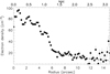 |
Fig. 6. Radial profile of the electron density derived from the ratio of the [S II] 6717 Å and 6731 Å lines calculated with pyneb (Luridiana et al. 2015). The dashed line shows the fitted radial profile of the density as explained in Sect. 5.1. |
In the radial profile, the density drops from a maximum value of around ne = 100 cm−3 in the centre of ESO 338 to values below ne ≈ 10 cm−3 where the densities become difficult to measure as the line ratio approaches the asymptotic value. The central 0.5″ shows a lower density due to the bubble evacuated by cluster 23 (Östlin et al. 2007).
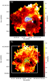 |
Fig. 7. Ionization structure of the halo of ESO 338. Panel a: ionization parameter map of the central area of ESO 338 as traced by the [O III]λ 5007 Å/[S II] λ(6717 + 6731) Å line ratio. The blue contours show the He II λ4686 Å emission. The He II image was smoothed with 3 pixel Gaussian kernel. The contour levels range from 50 to 1300 × 10−20 erg s−1 cm−2. Panel b: ionization map as derived from the [O III]5007 Å over Hα line ratio. The black contours are the I-band contours similar to Fig. 4. The white box denotes the borders of the slightly zoomed in [O III]/[S II] ionization map in panel a and the extinction map in Fig. 5. |
4.4. Degree of ionization
In Bik et al. (2015) two ionization cones were identified based on the [[S II]]/[O III] line ratio. With the new dataset we are able to probe the physical properties even further out in the halo. Panel a in Fig. 7 shows the deeper [O III] over [[S II]] map (inverted with respect to Bik et al. 2015). Apart from the ionization cones to the north and the south and the very ionized central region, the more neutral areas east and west of the central star burst become more evident. This area in the halo coincides with the location of the older stellar populations, characterized by a strong Hβ absorption (Sect. 4.1).
Another signature that becomes evident by tracing the outskirts of the halo is that the ionization increases again beyond 3.5 kpc, as shown in Fig. 7, panel b, where the ratio of [O III] and Hα is plotted. These are the two strongest lines in our MUSE data, and therefore also trace the halo to the largest size. In the area where both maps overlap, the same features are visible, suggesting that [O III] over Hα does mostly trace the ionization and to lesser extend abundance variations in [O/H].
Pellegrini et al. (2012) relate the [O III]/[S II] ratio to the optical depth of LyC photons by applying photoionization modelling. They show that at low optical depths the low-ionization line ([S II]) is suppressed with respect to the high-ionization line. Only at higher optical depth, the [O III]/[S II] ratio will decrease towards the edges of the H II region, resembling a classical Strömgren sphere and the H II region remains ionization bounded (LyC photons are captured).
In Fig. 7, the central area of ESO 338 is highly ionized, showing very high ratios in both [O III]/[[S II]] and [O III]/Hα. Then the ratio drops to [O III]/Hα = 1.3 until 3.5 kpc from the centre. At radial distances larger than 3.5 kpc, the ionization of the halo goes up again. This is especially visible in the north of the halo. The southern ionization cone also shows a very strong rise of the ionization after 3.5 kpc. In the northern halo, also an elongated feature of low-ionization is visible towards the north-west.
The decrease in [O III] over Hα at radii less than 3.5 kpc is analogue to an HII region around a star, the O++ zone is smaller than the H+ due to the fact that few O+ ionizing photons are available (hν > 35.2 eV) than H ionizing photons (hν > 13.6 eV). The radial increase at larger radii can be explained by several possibilities. The first explanation is that due to the fast dropping off gas density (Fig. 6) the mean-free path of the ionizing photons becomes large and the rate of recombinations does not balance anymore the rate of ionizations, resulting in a higher ionization fraction of the gas. This indicates that the halo is density bounded instead of ionization bound, and would suggest that ESO 338 is leaking LyC photons (also found by Leitet et al. 2013). Also shocks can cause an increase in ionization and fast radiative shocks can result in emission of high ionization lines such as Ne V and He II (Izotov et al. 2001; Thuan & Izotov 2005; Herenz et al. 2017). As will be discussed in Sect. 5.2, we do find evidence for shocks around the central starburst , however, in the other regions where we find the increase in [O III]/Hα ratio, the full-width at half maximum (FWHM) is rather low, suggesting that shocks might not be important here. A third possibility is presented by Binette et al. (2009), where they model gas turbulent mixing layers. Warm photoionized condensations are immersed in a hot supersonic wind resulting in turbulent dissipation and mixing, accelerating and heating of the gas. This can lead to an increase of the [O III]/Hα ratio. The condensations will be of higher density and therefore have a higher optical depth for the LyC photons, however, the lower density gas in which the condensations are immersed still enables the escape of LyC photons.
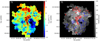 |
Fig. 8. Kinematic information derived from a Gaussian fit to the Hα emission with the Hα velocity field (left panel). The black contours are the contours of the I-band image reconstructed from the MUSE cube. Right panel: FWHM map of the Hα line. The instrumental FWHM is quadratically subtracted. Over-plotted in blue and red contours are the blue (−50, −30, −15 km s−1) and red (15, 25, 35 km s−1) shifted velocity respectively. |
Tracing even higher energetic photons are the emission lines from He++ recombination (hν > 54.4 eV). Over-plotted on panel a of Fig. 7 is a contour map of the He II emission. Apart from the broad He II emission peaking on some of the cluster positions (Sect. 3), there is a lot of spatially extended, diffuse He II emission. This diffuse emission has a narrow spectral profile and is of nebular origin. We detect diffuse He II emission in the central area of the galaxy. In this area most of the young clusters, including the WR cluster (Sect. 3.2), are found. The He II emission also overlaps with an area of high [O III]/[S II] ratio, suggesting very high ionization. This indicates that the He II is originating from photoionization by O stars and WR stars, that are also contributing to the high [O III]/[S II] ratio.
4.5. Kinematics
In order to derive kinematic information such as the velocity and velocity dispersion, we applied a Voronoi pattern to the integrated Hα emission line map with a minimum S/N of 20 and a maximum cell size of 900□ pixels (36□″). This pattern is applied to the reduced data cube and we fitted the Hα line in each Voronoi cell with a Gaussian profile.
Figure 8 shows the results in both the velocity map as well as the map of the FWHM. The systemic velocity for ESO 338 is adopted to be 2841 km s−1, as discussed in Bik et al. (2015). The FWHM of the instrument line spread function (LSF) at the observed wavelength of Hα is calculated using the formulas given in Sect. 5.2 of Bacon et al. (2017). Bacon et al. (2017) derive the FWHM of the LSF as function of wavelength by fitting a large number sky lines over the entire MUSE field of view. At the wavelength of the redshifted Hα emission (6625 Å), the FWHM of the LSF is found to be 114.5 km s−1. Because of the overall stability of the instrument no significant changes in the spectral resolution are expected to occur. However, we checked this value on our data by measuring the FWHM of the Xe λ 6595.56 Å arc line (close to the position of Hα) in a reconstructed cube of an arc frame. The measured mean FWHM over the field of view of the instrument of the line is 114 km s−1, with a standard deviation of 9 km s−1, consistent with value derived by Bacon et al. (2017). We quadratically subtracted the 114.5 km s−1 instrumental FWHM from the observed FWHM map.
With the two datasets combined we can measure the velocity field and the FWHM as far as ∼40″ (7 kpc) and both the velocity map and FWHM reveal many more structures than already discussed in Bik et al. (2015). In Bik et al. (2015) we already presented the redshifted elongated features starting from the central area of the galaxy and extending north and south. Additionally, Bik et al. (2015) shows that the gas in the northern redshifted feature is highly ionized and conclude that these are outflows driven by feedback from the clusters in the central area of the galaxy. The new velocity maps shows that the north-western outflow, in contrast was what seen in Bik et al. (2015), does not extend to the end of the halo. It extends to a distance of 3.6 kpc. We will discuss the outflow feature in more detail in Sect. 5.4.
Further to the north-west of halo the velocity field turns chaotic with small patches showing blue shifted velocities and other patches showing redshifted velocities. The velocity difference between two patches can be as high as 60 km s−1. North of the northern outflow feature, the velocity becomes again redshifted with a velocity of 30 km s−1. Also in the southern part several blue and redshifted features can be seen in the velocity map.
West of the starburst there is a large area with strongly blue shifted Hα emission, with velocities up to −60 km s−1. A similar blue shifted component is also visible in the velocity map of the H I emission (Cannon et al. 2004). This blue shifted region is not very bright in Hα, while it is one of the brightest regions in H I, rising the suggestion that this region is predominantly neutral. Inspecting the HST continuum images, we find that there is some star formation associated with this region, located just east of the bright foreground star. This region, a bit offset from the main starburst, contains a handful of 104 M⊙ clusters between 1 and 6 Myr, making this region to stand out in the ionization maps (Fig. 7) and show nebular He II emission. However, the star formation, and He II emission, is very localized and at the edge of the blue shifted feature. The main part of this feature shows low ionization in the ionization maps (Fig. 7). The feature is not very collimated and also the strong H I emission suggests against it being an ionized outflow created by the stellar feedback. We do not observe an increase in the FWHM. If this cloud would be in-falling in the galaxy, an increase in FWHM would be expected due to the super position of the in-falling cloud and the gas in the galaxy it self. Therefore we conclude that this cloud must be part of the galaxy ISM and possibly part of a perturbed disk of the galaxy. We speculate that this cloud is a remnant of an in-falling cloud which triggered the current starburst.
The velocity field of ESO 338 is so perturbed that there is no clear signature of rotation in the halo. Based on Hα Fabry–Perot observations, Östlin et al. (1999, 2001) derived rotation curves for a sample of BCG galaxies that included ESO 338. They did not manage to derive a proper rotation curve for ESO 338 as the observed velocity gradient along the body of the galaxy is not symmetric due to the strong blue shifted emission. In our MUSE velocity map we have more information than in the Fabry–Perot maps, however, also in the MUSE maps, there is no real rotational profile detected.
The map of the velocity dispersion shows, similar to the velocity map the complexity of the ionized halo of ESO 338. In general the FWHM shows rather large values in the halo (∼100 km s−1), much higher than the thermal broadening. A detailed comparison between the FWHM map and the velocity map shows that the two redshifted feature interpreted as outflows also show high velocity dispersion, especially at the location where the redshifted emission end (see Sect. 5.4). In the northern part of the halo, in between the red-shifted outflow and the redshifted regions further north, the FWM increases strongly. In the north-western part of the halo the chaotic velocity field also corresponds with a similar behaviour in FWHM map, where some patches have broad lines and others quite narrow. More to the north, however, the velocities become ordered again, also resulting in a decrease of the FWHM. Additionally, south and south east of the central area hosting all the young clusters an increase of the FWHM is observed in a ring like structure.
In order to see whether ordered or random motions dominate the kinematics and to compare ESO 338 to high-redshift observations, we calculated the ratio vshear/σ0. Where vshear is half the difference between the minimum and maximum velocity measuring the large scale motions in the galaxy and σ0 is the flux weighted average of the velocity dispersion, measuring the random motions in the galaxy. We used the procedure described in Herenz et al. (2016) to derive the two quantities.
We find that vshear = 28.4 km s−1, and σ0 = 57.5 km s−1, making the ratio vshear/σ0 = 0.5. These values suggest that the kinematics in ESO 338 are highly dispersion dominated (Glazebrook 2013). This is a property found among more blue compact galaxies (Östlin et al. 2001) as well as high-redshift star forming galaxies (Newman et al. 2013). The energy released by the stellar feedback increases the turbulence in these galaxies resulting in larger velocity dispersion.
5. The ionized halo of ESO 338
The Hα line map (Fig. 4) shows that the ionized gas around ESO 338 fills the entire FOV of the observations. In this section we study the halo in more detail and derive the total mass of the ionized gas as well as perform a spatially resolved BPT analysis of the ionized gas in the halo. Finally we look closer at the features identified as outflows in the halo of ESO 338.
5.1. Ionized gas mass
In order to derive the mass of the ionized gas, we constructed a surface brightness (SB) profile of the Hα emission (Fig. 9) by radially averaging the emission. The centre of the profile is, as for the radial density profile, chosen to be the location of cluster 23. The SB profile is measured as far out as 9 kpc, with a dynamic range of about 106.
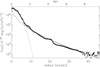 |
Fig. 9. Radial surface brightness profile of the Hα emission line. As central position, the position of cluster 23 has been chosen. Over plotted is a fit to the profile (solid line), consisting of a central Gaussian (dotted line) with σ = 2.38 ″ (0.50 kpc) and a Sérsic profile with an index of 1.8 to fit the extended halo with a scale length of 0.54″ (0.11 kpc). |
After a relatively constant central surface brightness, between 5 and 10″ (2 kpc) the SB profile drops rapidly and flattens beyond 10″ and drops more monotonically to low values. This SB profile can be fitted with a combination of a Gaussian profile in the centre and a Sérsic profile at larger radii. For the Gaussian in the central areas we measured a σ of 2.38″ (0.50 kpc). This emission likely is originating from the central starburst in ESO 338. The outer halo can be well described by a Sérsic profile with index n = 1.8 and a scale length of 0.54″ (0.11) kpc. This profile describes the SB profile reasonably well down to faint SB levels (Fig. 9). However, this is not a unique fit, the profile can also be explained by a central Gaussian and two exponential profiles. An exponential profile with a short (2.2″) scale length, dominating between 10″ and 20″ and an exponential with a longer scale length (8″) representing the SB profile beyond 20″. The derived surface brightness profile of ESO 338 is similar to what is found for other BCGs, where typically a central core with a exponential envelope is observed (e.g. Papaderos et al. 2002; Papaderos & Östlin 2012, Östlin et al., in prep.).
From the observed Hα SB profile and the radial density profile, derived in Sect. 4.3, we can derive the mass of the ionized halo around ESO 338. The mass of the ionized gas is related to the Hα luminosity and electron density as follows:
 (1)
(1)
where μ is the atomic weight, mH is the hydrogen mass, LHα,0 the extinction corrected Hα luminosity, h is Planck’s constant, νHα is the frequency of Hα and  is the Case B recombination coefficient for Hα, and ne is the electron density. For μ, a values of 1.0 is chosen, and
  is for a 1.2 × 10⁴ K gas equal to 9.835 × 10⁻¹⁴ cm3 s−1 (Pequignot et al. 1991).
The Hα luminosity is derived assuming a luminosity distance of 37.5 Mpc (Östlin et al. 1998). The observed luminosity is corrected for extinction by making a radial E(B – V) profile assuming the Prevot et al. (1984) extinction law. This profile is roughly constant through the halo with an average value of E(B − V) = 0.063 ± 0.05 mag. We derived this value by averaging the central 20″ of the extinction radial profile. The error is chosen to reflect the radial profile further out and is derived by quadratically averaging the error between 0″ and 40″.
We do not measure the radial profile of the electron density as far out as we do for the Hα SB profile. In order to extrapolate the electron density radial profile beyond 15″, we made an assumption about the shape of the radial profile. Assuming the Hα emission is emitted by recombination, the Hα luminosity is proportional to the square of the electron density ( ). When we assumed that the Hα luminosity profile drops as a Sérsic function with a certain scale length and index n = 1.8, the density radial profile would follow a Sérsic function with the same index n, but with a scale length which is 3.48 times larger (1.88″). The absolute scaling of that Sérsic profile was determined by fitting that function to the observed density profile between 6″ and 11″ (dashed line in Fig. 6).
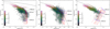 |
Fig. 10. Spatially resolved BPT diagrams of the ionized gas around ESO 338. Left panel: “classic” BPT diagram [N II]6583 Å/Hα vs. [O III]/Hβ (Baldwin et al. 1981), middle panel: [S II]/Hα vs. [O III]/Hβ diagram, and right panel: [O I]/Hα vs. [O III]/Hβ (Veilleux & Osterbrock 1987). The data points are colour-coded according to their Hα flux in a logarithmic scaling. The areas where the [O III] or Hα emission is saturated are excluded from the diagram. The green asterisk is the flux weighted average of all the data. The dashed line in the [N II] diagram shows the Stasinska et al. (2006) divisory line between star-forming galaxies and AGNs, while the solid line shows the divisory line from Kewley et al. (2001). In the two other diagrams the solid lines separate the star forming galaxies from AGNs according to Kewley et al. (2001). The red dashed (constant magnetic field) and blue solid (constant velocity) lines are predictions from fast radiative shock models by Allen et al. (2008), calculated for different magnetic field strength and shock velocity. Only the shock + precursor models with the SMC metallicity are plotted. |
For each radius we calculated Eq. (1). We do the calculations only for the fit with the Sérsic profile with n = 1.8. For the 3 component profile with two exponentials, the derived values are very similar. Summing up over all radii gave a total hydrogen mass M(HII) = 3.0 × 10⁷ M⊙. We also derived the total Hα luminosity corrected for extinction to be LHα = 3.56 ± 0.06 × 1041 erg s−1. The error on the measured LHα is dominated by the error on the extinction. The error on the total hydrogen mass is hard to determine as the derived value depends very strongly on the extrapolated radial profile for the electron density. The derived extinction corrected Hα luminosity corresponds to a star formation rate (SFR) for ESO 338 of 1.9 M⊙ yr−1, adopting the calibration of Kennicutt & Evans (2012). We note that this value strictly only valid under the assumption of a continuous star formation rate and no LyC leakage. The star formation rate derived from Hα is sensitive to the stellar population with an age between 0 and 10 Myr, with 3 Myr as the the mean age of the stellar population contributing to the Hα emission (Kennicutt & Evans 2012). Östlin et al. (2003) and Adamo et al. (2011) derive the star- and cluster formation history of ESO 338 and show that this is strongly rising with time. However, at very young ages this becomes very uncertain as the SED fits to the youngest clusters are subject of many uncertainties in the models. In the case of a rising star formation history we would slightly over estimate the actual current star formation rate. On the other hand effects such as absorption of LyC photons by dust, leakage of LyC photons will under estimate the derived star formation rate (e.g. Otí-Floranes & Mas-Hesse 2010).
We can compare the derived values to previous work by Östlin et al. (1999, 2009). Östlin et al. (1999) measured the Hα luminosity from Hα Fabry–Perot observations and found a luminosity of 4.9 × 1034 W (4.9 × 1041 erg s−1). A similar value was found by Östlin et al. (2009) from HST Hα imaging. These values are a bit higher than the total luminosity derived from the MUSE emission line map (3.56 ± 0.06 × 1041 erg s−1). However, the total mass we derived is five times lower than derived by Östlin et al. (1999); 1.6 × 10⁸ M⊙, assuming a constant density of ne = 10 cm−3. From the MUSE data we have derived a more realistic density profile, which is higher than 10 cm−3 in the inner 12″ of the halo. Inside this radius, also most of the Hα flux is emitted. As the mass scales with the inverse of the electron density (Eq. (1)), the derived mass will be lower with a higher electron density.
Also the SFR we derive is lower than the 3.2 M⊙ yr−1 calculated by Östlin et al. (2001). This is partly due to our lower Hα luminosity and partly due to different conversions used. We used the conversion from Kennicutt & Evans (2012) assuming a Kroupa & Weidner (2003) IMF while Östlin et al. (2001) used their own conversion with a Salpeter (1955) IMF.
Compared to the mass of the neutral hydrogen (1.4 ± 0.2 × 10⁹ M⊙) derived from H I observations by Cannon et al. (2004), the derive ionized gas mass is only 1% of the total halo mass. This indicates that the halo around ESO 338 is predominantly neutral and which could have implication for the escape of LyC photons from this galaxy.
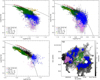 |
Fig. 11. Spatially resolved BPT diagrams of ESO 338 (see Fig. 10). The different colours represent different selections made in the BPT diagrams. Red: data points with a very high [O III]/Hβ ratio, selected in the SII diagram as being above the star formation line, but not originating in shocks log([S II]/Hα) < −0.8. Green: high ionization (log([O III]/Hβ) > 0.4), star formation dominated gas (selected in the [O I] diagram). Blue: data points which cover the same area in the [O I] diagram as the shock models of Allen et al. (2008) and are located above the star formation line. Pink: low-ionization (log([O III]/Hβ) < 0.4), star formation dominated gas selected in the [O I] diagram. Orange: nitrogen enhanced gas detected as high [N II]/Hα ratio in the [N II] diagram. Black: data points which do not fulfil any of the selection criteria. Bottom right panel: in greyscale the [O III]/[S II] line ratio, tracing the ionization (Fig. 7) with over-plottted the location of the different selections made in the BPT diagrams. |
5.2. Spatially resolved BPT diagrams
In order to gain insight in the ionization processes of the ionized ISM and halo of ESO 338, we constructed emission line ratio diagrams (BPT diagrams, Baldwin et al. 1981; Veilleux & Osterbrock 1987). The location in the BPT diagram is a function of many parameters, such as ionization, metallicity, electron density and hardness of the radiation field (e.g. Kewley et al. 2006), allowing us to trace these properties in a spatially resolved manner.
We constructed three different BPT diagrams, all having the [O III]5700 Å/Hβ ratio on the y-axis. We show the [N II]6583 Å/Hα (referred to as the [N II] diagram), originally presented in Baldwin et al. (1981). Additionally, the BPT diagrams with [S II](6713 + 6731) Å/Hα ([S II] diagram) and [O II](6300) Å/Hα ([O I] diagram) originally presented in Veilleux & Osterbrock (1987) will be discussed.
In order to construct the different BPT diagrams, we applied Voronoi binning to increase the S/N in the outskirts of the halo. For each diagram, we select the faintest emission line to calculate the Voronoi pattern (see Table 3). The Voronoi pattern is calculated ensuring a minimum S/N of 20 per cell and a maximum cell size of 900□ pixel (36□″). The pattern is then applied to the other emission line maps required to construct the BPT diagram. This procedure results in a different Voronoi pattern for each BPT diagram as the faintest emission line is a different one for each of them. For this reason the BPT diagram with [O I] (the faintest line) has less data points than the other two diagrams. For the [S II] diagram we have a total of 39 049 cells, for the [N II] diagram we have 26 536, while for the [O I] we have 21 905 cells.
The line ratios calculated in each Voronoi cell represent a point in the BPT diagram (Fig. 10). We also show in these diagrams the division lines between star forming galaxies and active galactic nuclei (AGN) from Kewley et al. (2001) and, only in the [N II] diagram, also the divisory line from Stasinska et al. (2006). As a green asterisk the location of the flux weighted average of all the data points is shown. The green asterisks show the position in the diagrams if the line ratios are calculated from summing all the measured flux in each emission line. The location of the green asterisk is consistent with previous determination of the position of ESO 338 in the BPT diagram (Bergvall 1985; Leitet et al. 2013). The green asterisks are all located in the upper left part of the BPT diagram, consistent with ESO 338 being a low-metallicity, high-ionization galaxy.
In the [N II] BPT diagram all data points are located well below the star formation line of Kewley et al. (2006), suggesting that photoionization is the dominant ionization process. However, looking at the [S II] and [O I] BPT diagrams, many points are located above the star formation line, highlighting the importance of other emission mechanisms than photoionization. One of those possible other mechanisms are shocks in the ISM. Over-plotted in Fig. 10 are the model predictions for fast radiative shocks calculated with the MAPPINGS III code (Allen et al. 2008) for velocities between 200 and 500 km s−1. We only show the precursor + shock models for SMC metallicity, closest to the metallicity of ESO 338 (12 + log(O/H) ≈ 7.9, Guseva et al. 2012). These shock models explain the location of the points with the highest [S II]/Hα and [O I]/Hα ratios outside the star formation area in the BPT diagrams. Kewley et al. (2006), show that increasing the electron density and adding a more extreme UV field (caused by WR stars or very hot O stars) increase both the [O III]/Hβ and [N II]/Hα ratio. A higher ionization parameter will, in low-metallicity gas, result in an increase of the [O III]/Hβ ratio.
We have to be cautious when interpreting spatially resolved BPT diagrams, as the BPT diagram is originally used to separate star formation galaxies from AGNs dominated galaxies using integrated emission line spectra. Ercolano et al. (2012) shows that, based on a 3D magnetohydrodynamics simulation without shocks, a large fraction of the points may fall above the star formation line. The 2D projection of a 3D complex ISM can result in having both more neutral and highly ionized material along the line of sight. They show that this results in a high [O III]/Hβ ratio and a high [S II] or [N II] over Hα ratio, moving the point to the upper right area of the BPT diagram mimicking the presence of shocks.
To study the nature of the different components in the BPT, we apply several selections in the different BPT diagrams and identify the spatial location of those points in the halo. Figure 11 shows the three BPT diagrams again, but now with different selections described below:
High [O III]/Hβ (red triangles). In both the [S II] and [O I] diagrams we find points with a very high [O III]/Hβ and low [S II]/Hα or [O I]/Hα. In the [N II] diagram they can be seen as a sequence above most of the data points between log([N II]/Hα) = −1.8 and −1.6. We selected these high [O III]/Hβ data points, located above the star formation locus. We used the [S II] diagram where they form the clearest sequence separated from the main cloud of points. The points are selected to have a [O III]/Hβ of at least 1.07 × the ratio of the separation between star formation and AGN. This ratio is chosen such that it separates the sequence from the other data points. Additionally, we select only those points which have a log [S II]/Hα ratio less than −0.87.
Shocks (blue squares). We selected all data points that overlap with the shock models of Allen et al. (2008) and are located above the star formation line. We make this selection in the [O I] diagram where the displacement from the star formation locus is the largest.
Low-ionization star formation (pink diamonds). These points are selected in the [O I] diagram with log [O III]/Hβ < 0.4 and located within the star-formation locus.
High-ionization star formation (green dots). The points representing more highly ionized gas inside the star formation locus are selected in the [O I] diagram to have [O III]/Hβ > 0.4.
Nitrogen enhanced gas (orange upside down triangles). This selection is made in the [N II] diagram. From log([O III]/Hβ) ratios between ∼0.6 and ∼0.75 several points with increased [N II]/Hα ratio compared to the bulk of the points at that [O III]/Hβ ratio are present. The high [O III]/Hβ points are selected by selecting point following relations [O III]/Hβ > −0.55[N II]/Hα −0.06 and [O III]/Hβ > 0.65, while the low [O III]/Hβ points are selected following [O III]/Hβ > −1.05[N II]/Hα −0.73 and [O III]/Hβ < 0.6. These points only stand out in the [N II] diagram, in both the [S II] and [O I] diagrams they are located mostly in the star formation locus and clearly do not stand out as a separate sequence. This indicates that these points represent locations with enhanced nitrogen abundance (Sect. 5.3).
As the selection is done in three different diagrams, points can be part of more than one selection. This concerns the high [O III]/Hβ (red) and the nitrogen enriched (orange) data points. All the other selections are done in the [O I] diagram. The high [O III]/Hβ data points do not overlap with any other selection, the offset between these points and the high-ionization star formation data points (green) is large enough to avoid overlap, also in the [O I] diagram. The nitrogen enriched data points do overlap with other selections. Almost all of these points are classified as high-ionization star formation (green) in the [O I] diagram.
A large number of data points are not fulfilling any of the selection criteria and are plotted as black points in Fig. 11. In the [O I] diagram they are located above the division line, but do not overlap with the shock models of Allen et al. (2008). In the other two diagrams, the black points overlap with the green (high ionization star formation) and blue (shocks) points. These points trace star forming gas as well as shocked gas or a mix of both. These points are likely located in between the central area dominated by star formation and the ring of shocked gas.
In the bottom right panel of Fig. 11 the location of the different selections discussed above are over-plotted on the grey-scaled plot of the [O III]/[S II] ionization map (Fig. 7). It shows that the central area of the galaxy where all the YSCs are located is dominated by highly ionized gas, photoionized by the massive stars in the clusters (green area). The green area extends towards the north-east and spatially overlaps with the outflow identified in the Hα velocity field (Bik et al. 2015), suggesting that the gas from the central areas is streaming out along the outflow cavity without producing strong shocks. The gas with the very high [O III]/Hβ ratio (red) is mostly located near cluster 53. This is one of the clusters identified as WR cluster in Sect. 3.2. The Hα emission towards the cluster is saturated (and masked out from the analysis), but just west of the cluster the gas shows the high [O III]/Hβ. The WR stars in this cluster are likely responsible for this very high ionization.
The low-ionization gas in the star formation locus (pink) is located in the eastern part of the galaxy where a relatively large Hβ absorption was found (Sect. 4.1). This suggests a somewhat older stellar population emitting much less ionizing photons than the young population in the centre. Also in the ionization maps (Fig. 7), this area is characterized by line ratios indicative of low-ionization.
The points outside the star formation locus and overlapping with the shock models (blue) are located in the outer regions of the halo. The spatial distribution of the shocked gas is in the shape of a ring around the starburst, with two openings where the ionization cones (and northern outflow) are located (Bik et al. 2015). This is suggestive of the halo gas outside the starburst being shocked by the expanding HII regions created by the stellar feedback. Following Ercolano et al. (2012) the points above the star formation divisory line can also be explained by overlapping low-ionization and high ionization H II regions. The area we see the shocked gas also shows lower ionization. We do see, however, also an increase in FWHM, this would be more suggestive of the presence of shocks.
5.3. Nitrogen enrichment
To study the location of the gas with a high [N II]/Hα ratio in more detail, we show in Fig. 12 the log([N II] (6583 Å)/Hα) image of the central area of ESO 338. The dark areas in this figure show the low [N II]/Hα ratio at the location of where the gas is highly ionized (N II is ionized to N III). These areas correspond to the green data points in the BPT diagrams (high [O III]/Hβ ratio) and corresponding to the location of the most massive star clusters. Apart from the dark areas, we also can identify several bright areas with high [N II]/Hα ratio. These [N II] enriched areas are marked with A, B and C in Fig. 12).
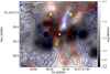 |
Fig. 12. Map of the log([N II]/Hα) ratio in the central areas of ESO 338, highlighting the features showing the increase in the [N II]/Hα ratio. A v-shaped feature (B) as well as a circular blob (A) are seen north of the starburst clusters, while a fainter elongated feature (C) can be seen extending to the south. Overlayed in blue (−30, −20, −10, 0 km s−1) and red (10, 20, 30 km s−1) contours is the velocity field of the [N II] 6583 Å line. The eastern leg of feature B shows a strong blue shifted emission, which is not seen in Hα. The white asterisk is the possible location of the responsible cluster for the nitrogen enrichment. |
Region A is north of most of the star clusters and is represented in the BPT diagram by the orange points around log([O III]/Hβ) ∼0.5 (Fig. 11). Region B has a v-shaped morphology and the brightest area of this region corresponding to the orange points around log([O III]/Hβ) ∼0.7 in the BPT diagram (Fig. 11). A much fainter enhancement (region C), elongated in southern direction is visible south of region B.
Nitrogen enhancement has been observed in several BCG galaxies (e.g. James et al. 2009; Monreal-Ibero et al. 2010, 2012; Pérez-Montero et al. 2011) towards WR clusters, suggesting that the emission is due to enrichment by WR stars (or very massive stars above 100 M⊙, which already show WR like stellar winds in a very early phase of their evolution, Smith et al. 2016). Region A has no corresponding continuum source detected in HST imaging, but is spatially coinciding with the outflow detected in Hα. The geometry of the two other features also suggests a relation to outflowing gas. Also here, the emission is not directly co-located with a clusters, however, in between region B and C several young clusters are detected.
To see if the enriched gas has the same velocity as the rest of the gas, we calculated the velocity map of [N II]6583 Å, applying a Gaussian fit (identical to the Hα line). The contours of the [N II] velocity field are overlayed on the [N II]/Hα line map (Fig. 12). Surprisingly, the eastern leg of region B shows a blue shifted velocity. This is not seen in the Hα velocity field (Fig. 8), where the gas is redshifted like the surrounding gas. We measure a maximum velocity of the [N II] emission line of −40 km s−1 (blue contours on Fig. 12), while the velocity measured from Hα is around +10 km s−1. We also find a region of increased [N II]6583 Å FWHM just east of region B, in between the blue shifted feature and the strongly redshifted feature just east of it, suggesting that we see both components overlapping resulting in a double line profile, not resolved by our MUSE spectroscopy.
The same features are also visible in the other [N II] lines present in the MUSE spectrum. Both the 6549 Å and the much fainter auroral line 5755 Å show the same pattern as the 6583 Å line, both in their ratio to Hα as well as in velocity, indicating that this is not a data reduction artefact. We have inspected several line ratio maps ([O III]/Hβ, [S II]/Hα, [O I]/Hα, He I/Hα, He II/Hα, [Fe III]/Hα) to see if enhancements in other elements other than nitrogen are present. None of the maps show the same features as the [N II]/Hα maps, suggesting that the gas is only enhanced in nitrogen. This makes the enhancement by supernovae unlikely, as supernova remnants are typically bright in [S II] (Blair et al. 2012). The fact that these nitrogen enriched regions are highly ionized (high [O III]/Hβ) supports the hypothesis that this is gas enriched by WR stars.
As the geometry of regions B and C are elongated, this gas could be outflowing gas. We can see in Fig. 12 that region B in the north and region C south are connected by an area with very low [N II]/Hα (high ionization). Inside this area of high ionization we find three bright clusters: clusters 27, 28 and 29 from the inner sample of Östlin et al. (1998). All three clusters have masses of ∼3 × 10⁵ M⊙. Assuming a covering fraction of 0.5, the ages are 6 Myr for cluster 27 and 28 and 10 Myr for cluster 29. These clusters are a bit too old for clusters containing WR stars at low metallicity. We also do not see the WR features towards these clusters. The clusters in which we identify the WR features (Sect. 3.2) are not associated with the areas of nitrogen enrichment and they are also younger than the clusters we identify in between region B and C. An explanation for this apparent discrepancy can be related to the fact that the gas is outflowing. It will take some time before the gas is travelling away from the clusters and by the time we observe the enriched gas, the WR stars have already disappeared.
5.4. The galactic outflow
We matched the derived ISM properties from the MUSE data to the high-resolution HST data, in order to spatially characterize the outflow identified in the MUSE Hα velocity map. Figure 13 shows the HST continuum subtracted Hα image from Östlin et al. (2009) with the red shifted and blue shifted velocities from the MUSE Hα velocity map overlayed as contours (Fig. 8).
At the high spatial resolution of the HST, the Hα image shows the evacuated bubble around cluster 23. The location of cluster 23 is associated with the point source in the middle of the bubble. The edges of the bubble do not show a uniform brightness and towards the north, the bubble seems to be open. As already noted in Bik et al. (2015), the velocity contours in Hα show that the northern outflow is a complex or probably multiple outflows. A comparison with the HST Hα image suggests that cluster 23 is likely responsible for the most eastern part of the outflow, the base of that part of the outflow overlaps with the open side of the bubble (Fig. 13). The stellar wind and supernova feedback form cluster 23 is responsible for creating the bubble. The fact that the bubble is open and a large scale outflow is driven from this bubble can be explained by the standard model of galactic winds (e.g. Chevalier & Clegg 1985; Heckman & Thompson 2017). Due to the mechanical energy input of the stellar winds and supernovae, a bubble is created and the gas inside the bubble is heated up and thermalized. Due to Rayleigh-Taylor instabilities, the bubble bursts and the hot gas streams out creating the galaxy scale outflow.
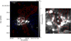 |
Fig. 13. HST continuum corrected Hα image taken from Östlin et al. (2009), with the red shifted and blue shifted MUSE Hα velocity map overlayed as contours (Fig. 8). The red contours show the velocity contours of 20, 30 and 40 km s−1, while the blue contours show the velocities −10, −20 and −30 km s−1. The zoom in shows the central 1□ kpc around cluster 23. The HST map shows the bubble around cluster 23 and the hole in that bubble towards the north. |
To analyse the gas in the outflow cones in more detail, we derived radial profiles from the northern and southern outflow cone in several emission lines (as indicated in Fig. 14c). The radial profile is constructed starting from the position of cluster 23. Our aim is to relate the measured velocities of the outflow with ISM properties such as the presence of shocks and the density profile. If we would derive the kinematic information from a similar radial profile as the ISM properties, the velocity variation would be heavily diluted at larger radii due to the high amount of structure in the velocity map. Therefore we create two pseudo long-slits with a width of 5 pixels (1″), one covering part of the northern outflow and one covering the southern outflow. This slit has roughly the size of the seeing during the observations and preserves most of the details in the kinematics. The slits are indicated in Fig. 14c.
Panels A1 and B1 show the FWHM (open diamonds) and the velocity (filled circles) profile along those long-slits. The northern outflow (panel A1) shows an outflow velocity varying between 20 and 50 km s−1 over a projected distance of 3 kpc with the highest velocities measured between 2 and 3 kpc. The FWHM shows a peak near the centre and then drops to a value of 100 km s−1 at 200 pc from cluster 23. This peak is not spatially resolved in our MUSE data and likely originates from the gas inside or at the edge of the bubble around cluster 23, suggesting a very turbulent nature of the gas. The same can be seen in the southern outflow (panel B1). At larger distances the FWHM in the northern outflow slowly increases again to values between 120 and 150 km s−1. At a distance of 3 kpc, where the drop in velocity suggests that the outflow ends, the FWHM of the gas increases even further to values up to 170 km s−1. The southern outflow does not show this effect at the end of the outflow. In this outflow, after initial increase in velocity to ∼50 km s−1 at 1 kpc, the velocity slowly decreases and at 2.5 kpc really drops to ∼0 km s−1. The FWHM varies strongly in the first 2 kpc, after which it slowly decreases to ∼80 km s−1 at 3 kpc distance from cluster 23.
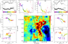 |
Fig. 14. Derived outflow properties. Panel C: zoomed-in Hα velocity map, where we have outlined the northern (panel A) and southern (panel B) outflow zones in which we derive the outflow properties. Additionally, two lines (with a length of 3.5 kpc each) are plotted from which we calculated an artificial long slit spectrum (5 pixels wide) in order to plot the kinematic information. Panels A1 –A4: extracted information for the northern outflow, and panels B1 –B4: information for the southern outflow. Panels A1 and B1: kinematic information (top FWHM, bottom velocity) extracted from the long slits as a function of distance from cluster 23. The colour bars at the bottom give the relation between colour and distance used in the remaining diagrams. The vertical dotted lines mark the positions of the extracted FLAMES Hα profiles (Fig. 15). Panels A2 and B2: BPT diagram log[O I]/Hα vs. log[O III]/Hβ, with the ratios as a function of radius derived from the radial profiles of these lines. Panels A3 and B3: log [O I]/Hα ratio vs. FWHM as a function of radius (colour-coded). Panels A4 and B4: radial density profile derived from the [S II] line ratio calculated using Pyneb. Over-plotted as dotted line is a r−2 power-law as predicted for galactic scale outflow (Chevalier & Clegg 1985). |
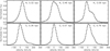 |
Fig. 15. High resolution Hα profiles of selected positions in the halo as observed with FLAMES. Top panels: Hα profile at 3 locations in the northern outflow, and bottom panels: corresponding profiles along the southern slit. These locations correspond to 3 points on the long slit defined in Fig. 14. The distances are given along the slit and are measured from the position of cluster 23 as in Fig. 14. |
Panels A2 and B2 show the [O I] BPT diagram (see also Fig. 10) of the radially averaged data in the outflow cones. The colours of the data points represent the distance from cluster 23 (see panel A1 and B1 for the relation between distance and colour). Most points are located below the line separating star forming galaxies and AGNs (Kewley et al. 2001). Close to cluster 23, the points are located in the upper left part of the diagram, suggesting high ionization. The points move down with increasing radius following the separation line, after a certain distance the points cross the line and occupy the region of the BPT diagram dominated by shocked gas.
For the northern outflow the points beyond 2.5 kpc are located in the shocked regime, which coincides with a strong increase in FWHM at the same distance. A similar effect can be seen in the southern outflow from 1.2 kpc, where at the largest FWHM, the points are located in the shocked regime of the BPT diagram.
These shocked areas are not seen in the spatially resolved BPT analysis (Fig. 11). Due to the radial averaging we are able to trace the gas properties out to much further distances than in the spatially resolved BPT analysis. The shocks appear outside the area covered in Fig. 11.
The relation between the log([O I]/Hα) and the FWHM is shown in panels A3 and B3. These panels show indeed that when the [O I]/Hα ratio becomes larger, also the FWHM of the lines increases. This is also seen for other galactic scale outflows (Heckman et al. 1990). This is especially clear in the northern outflow where the points at the end of the outflow show an increased FWHM and are also located above the separation line. In the southern outflow, the points between 1.2 and 2.5 kpc show a high FWHM, at these distances, the points are also above the separation line in the BPT diagram. Then at large radii, the FWHM slowly drops (as does the velocity), however, the log([O I]/Hα) remains high.
Finally, Figs. A4 and B4 show the radial density profile derived from the [S II] ratio for the two outflow cones. The dotted lines show the the r−2 relation expected for a galactic scale outflow (Chevalier & Clegg 1985; Heckman et al. 1990). The observed density profiles show similar behaviour as those observed by Heckman et al. (1990). In the centre of ESO 338 they show a roughly flat profile, tracing the density of the gas inside the starburst region and the individual HII regions. The increase at very short distance from cluster 23 is tracing the ring around the bubble (see Fig. 13). After that the density sharply drops consistently with the r−2 relation observed in other starburst (Heckman et al. 1990) and with the theoretical production of galactic winds (Chevalier & Clegg 1985).
In order to derive the dynamical age of the outflows, we need to have an estimate of the inclination under which we see the galaxy and the outflow. As shown by the analysis of Östlin et al. (1999, 2001), the velocity field is so perturbed that, if even present, a rotation curve could not be derived, making it hard to get a handle on the inclination of the galaxy. Östlin et al. (2001) estimated the inclination of the disk of the galaxy to be 55°. Assuming that the outflow is launched perpendicular to the disk plane, this would mean an outflow angle of 35° (angle ϕ in Heckman et al. 1990).
From our MUSE data we can derive some constraints; the observed velocities of the outflows are very low compared to other starburst galaxies The maximum velocity we measure is around 50 km s−1, while for local starburst galaxies Hα outflow velocities of several 100 s of km s−1 are common (Heckman et al. 1990). Assuming that outflow velocities are similar would suggest a low outflow angle. Additionally, we observe only red shifted velocities in the outflows. This excludes the possibility that the angle is close to 0. Typically the outflow is in the form of a cone with a finite opening angle (Heckman et al. 1990; Westmoquette et al. 2009). Both walls of the opening angle are showing red shifted velocity, suggesting an angle larger than 0. The inclination derived by Östlin et al. (2001) and the resulting 35° angle for the outflow is consistent with the above constraint. Therefore, for the remainder of the paper, we adopt an inclination of 55° used by Östlin et al. (2001) and the resulting 35° angle of the outflow under the assumption that the outflow is launched perpendicular to the disk.
For the northern outflow we measure a line of sight velocity between 30 and 50 km s−1, this would then translate in a real velocity between 52 km s−1 and 87 km s−1 and spatial extend of 3.7 kpc. The line of sight velocity at the end of the outflow is 40 km s−1, resulting in a real velocity of 70 km s−1. Assuming a constant velocity with time, this results in a dynamical age of the outflow of 5 × 10⁷ yr. Comparing this dynamical age to the possible driving source cluster 23 shows that this cluster cannot be the driving sources as the age of cluster 23 is only ∼6 Myr (Östlin et al. 2007). Östlin et al. (2003) and Adamo et al. (2011) derive the star and cluster formation history of the recent starburst and find the most recent burst started ∼40 Myr ago and showed an enhancement between 20 and 30 Myr while the peak of the star formation activity is younger than 10 Myr. These velocities would be consistent with the outflow being created at the beginning of the starburst in ESO 338 and the mechanical energy accelerating the ISM is now maintained by the new generation of star clusters.
However, we have to keep in mind that the measured centroid velocity is derived from a Gaussian fit to a complex velocity profile, adding up all components present along the line of sight. Assuming that the Hα emission mainly arrises from the walls of the outflow cones, the measured velocity is an average from both side of the outflow cone. Even if the cones move at relatively high speed, the average, centroid velocity can still be very low, especially, with the relatively low spectral resolution of MUSE where low-flux high-velocity components will be easily missed.
The central region of ESO 338 is also observed with the GIRAFFE/Argus integral field spectrograph of the FLAMES instrument mounted on the VLT. The data, presented in Sandberg et al. (2013), centred at Hα are obtained with a spectral resolution of R ∼ 12 000, a factor of 5 higher than our MUSE spectra. We extract the FLAMES spectra at 3 location along the long slits defined in Fig. 14. The GIRAFFE/Argus field of view limits the analysis of the high resolution spectra to the central kpc of the galaxy. These spectra are presented in Fig. 15 and show a large diversity of line profiles. The northern outflows shows a double peaked profile with the red component increasing with velocity with distance. At a distance of 0.59 kpc from cluster 23, the two components have a projected velocity separation of 83 km s−1, translating to a velocity separation of 143 km s−1 assuming an outflow angle of 35°. The southern outflow shows a high velocity component at 0.36 kpc distance with a projected velocity of ∼150 km s−1, which would result in 260 km s−1 corrected for outflow angle. These high velocities observed in the FLAMES spectra also lead to much shorter dynamical time estimates.
For example the high velocity component at a projected distance of 0.36 kpc from the centre has a dynamical age of only 1.6 Myr. This again illustrates the complexity of the outflow in ESO 338. The observed outflow complex is likely driven by many star clusters with different ages, leading to different components with a different dynamical age. This is especially true for the northern outflow, where also several spatially resolved components are visible on the velocity map confirms this picture. Both high spatial and spectral resolution observations would be needed to separate the different components and link them to individual clusters.
6. Discussion
In this paper we presented deep MUSE integral field spectroscopy of the blue compact galaxy ESO 338-IG04. We found that the galaxy is surrounded by a large, low-density ionized halo extending as far as 9 kpc. We presented a detailed analysis of the large ionized halo surrounding this galaxy and investigate the effect of the stellar cluster feedback on the physical properties of the halo.
6.1. The ionized ISM of ESO 338
Using the optical emission lines we analysed the ionized halo and ISM of ESO 338. The central ∼1 kpc of the galaxy is dominated by the starburst and contains most of the massive young stellar clusters, including several with WR stars. The densities inside the region of the starburst are between 100 and 200 cm−3. Outside the central ∼1 kpc both the Hα emission and the electron density drop fast. The Hα surface brightness profile drops of with a Sérsic index of 1.8.
Analysis using the BPT diagram shows that the ionized gas becomes shocked outside the central starburst region. Similar results have been found by Fensch et al. (2016) in another dwarf galaxy. We find the shocked gas to be located in ring around the starburst, with openings where we detect the outflows and ionization cones. We also see an increase in FWHM of the Hα line in the inner 3 kpc of the halo. The points overlap in the [O I] BPT diagram with the fast shock models of Allen et al. (2008), more specifically those with shock velocities between 200 and 500 km s−1. These high velocities are not measured in the MUSE FWHM maps, however, analysis of the FLAMES spectra in some regions of the outflows shows the presence of faint, much higher velocity components. They are just not visible in the low resolution MUSE spectrum. Additionally the shocks will be on small spatial scales, unresolved by our MUSE data.
In our first paper on the MUSE data of ESO 338 we have identified two galactic scale outflows (Bik et al. 2015). Further analysis of the ISM lines in these outflows show a very complex spatial as well as velocity profile, suggesting that multiple clusters are responsible for driving the outflow. We also find evidence for shocks at the outer regions of the outflow.
ESO 338 is a galaxy with similar properties to the samples discussed in Heckman et al. (2015) where a detailed analysis of the outflow properties are done based on HST/COS absorption line spectroscopy. Several galaxies in their sample (e.g. NGC 5253, SBS 0335-052 and Haro 11) are classified as BCG, similarly as ESO 338. The SFR (1.9 M⊙ yr−1, Sect. 5.1) of ESO 338 is a typical value measured in the sample of Heckman et al. (2015). The outflow properties, however, are more difficult to compare as Heckman et al. (2015) uses absorption spectroscopy, where the centroid velocity of the warm ionized gas measured with the galaxy as background, while we measure the centroid of the emission line emitted in the same gas, but not restricted to the gas in front of the galaxy continuum. Following the trends between outflow velocity (vout and SFR an outflow velocity between ∼30 and ∼150 km s−1 could be expected for ESO 338. This is very similar to what we measure in the emission lines.
Our emission line results can be better compared to Marlowe et al. (1995) and Martin (1998) where similar star-forming galaxies are observed using Hα imaging and long slit spectroscopy. Both studies derive similar dynamical ages as we do for the kpc scale expanding super bubbles and filaments present in these dwarf galaxies. They use the observed rotation curve to derive an estimate of the escape velocity and compare that to the observed outflow velocity in order to determine if the outflowing gas will escape the galaxy. They find that in most cases the outflowing gas has a velocity below the escape velocity, suggesting that outflowing gas will most likely not escape from the galaxy into the intergalactic medium (IGM). It is therefore suggested that these galaxies have not yet developed full fledged galactic scale winds where gas is escaping in the IGM.
The super-bubbles are created by the combined mechanical output of the stellar winds and supernova, in which the energy input of the supernova thermalizes the gas with a temperature up to 107 K. This gas will be very low density, but due to the high temperature still have a much larger pressure than the surrounding 104 K gas we trace with MUSE. This hot super bubble will therefore expand in the warm gas and create shocks visible as gas with an enhanced [O I]/Hα ratio similarly to the ring of shocked gas seen in the ISM of ESO 338 at ∼3 kpc from the centre. This ring can be caused by the expansion of the hot gas in a large super bubble surrounding the current starburst.
For ESO 338 we do also observe what looks like a more developed galactic scale wind. However, the outflow velocities are still rather low, which could mean that also for ESO 338 this gas does not escape from the galaxy. Due to the disturbed velocity field of the halo of ESO 338 it is not possible to derive a rotation curve of this galaxy in order to trace the gravitational potential and derive an escape velocity (see Östlin et al. 1999). However, assuming a spherical gravitational potential we can derive an estimate of the escape velocity.
We use the relation for vesc as function of radius and the mass of the galaxy derived by Marlowe et al. (1995). Assuming a spherically symmetric isothermal potential with an outer cutoff at rmax, the escape velocity at radius r can be expressed as  . For rmax we choose the Holmberg radius (V = 26.2 mag″2 isophote) for ESO 338 derived by Bergvall & Östlin (2002) to be 42″ (7.6 kpc). The circular velocity is estimated using the virial theorem, again assuming a spherically symmetric potential, as
  . For the mass we use the sum of the stellar mass (4 × 10⁹ M⊙, Östlin et al. 2001) and the H I mass (1.6 × 10⁹ M⊙, Cannon et al. 2004). This results in vcirc = 55 km s−1. The northern outflow has a de-projected length of 3.7 kpc. The escape velocity at this radius is vesc = 102 km s−1.
This value is a bit higher than the de-projected outflow velocity measured for the northern outflow (87 km s−1) and this would suggest that the outflowing gas does not escape. However, the assumption of a spherically symmetric gravitational potential is not realistic and the real escape velocity could be different. On the other hand, no dark matter is included in the mass estimate, making the value a lower limit.
From the radial velocity profile we can also see that both the northern and southern outflow did not reach (yet) the edge of the ionized halo. This means that at this moment, no gas is being expelled from the galaxy, if the outflow develops towards the edge of the halo it could eventually.
Because of the radial averaging we are able to trace the gas properties further out than in the spatially resolved analysis of the BPT diagram (Sect. 5.2). The radial averaging enables us to identify shocked gas at the end of the outflow traced by both an increase in the velocity dispersion as well as an increase in the [O I]/Hα ratio. Analogous to the case of the expanding super-bubble, this can be explained by the hot outflowing gas interacting with the more quiescent halo gas at the end of the outflow. Such an interaction would decelerate the outflow and create shocks at that location. Another explanation for the FWHM increase at the end of the outflow is related to the fact that the outflow expands in a lower density medium. The outflowing gas becomes very turbulent. Small scale shocks are created in the turbulent gas, resulting in an increase of the shock tracing lines.
6.2. WR stars and the origin of He II emission
We detected strong He II emission in ESO 338. Towards the WR clusters we detected broad He II 4686 Å emission, but we also find a spectroscopically narrow component. This narrow component is of more diffuse origin. The presence of narrow He II emission has been subject to multiple interpretations. He II emission requires the presence of a hard radiation field due to the high ionization potential of He++ (54.4 eV).
For galaxies at high redshift the narrow He II emission is even seen as a tracer of pop III stars (Cassata et al. 2013) as it is much stronger than the fluxes expected for WR stars and gravitational cooling radiation produced by gas accretion. In local galaxies, narrow He II emission is observed in the integrated spectra of several BCGs as well as low metallicity WR galaxies (e.g. Schaerer et al. 1999; Kehrig et al. 2008), suggesting that the emission is being caused by ionization from WR stars. Herenz et al. (2017) on the other hand, find evidence that the He II emission from the super shell structure in SBS0335-52E is created by an enhanced UV field caused by shocks in the shell.
In the case of ESO 338 we can see that the diffuse He II emission is located inside the central starburst containing also the WR clusters. The contours of the He II emission follow closely the areas of very high [O III]/[S II] and [O III]/Hα ratios, indication a high ionization (Pellegrini et al. 2012). Due to the lower-density winds in low metallicity environments (e.g. Smith et al. 2002), not only WR stars are responsible for the He II emission, but O stars could contribute significantly to the He II ionizing photon flux. It’s spatial distribution makes it likely that the He II emission in ESO 338 is caused by photoionization, with contributions from both the WR stars in the four clusters and massive O stars located in the younger clusters.
6.3. The origin of the nitrogen enhancement
The analysis of the BPT diagram and the [N II]/Hα ratio revealed several areas with enhanced [N II] emission (Sect. 5.3). We identified three distinct regions in the [N II]/Hα map (Fig. 12). Regions B and C seem to be linked to two clusters right in the middle of these regions with ages slightly older than typical WR clusters. The other, most northern region (region A) is difficult to trace back to a cluster, but has a velocity similar to the outflow detected in Hα.
In several BCGs nitrogen enhancements have been detected (e.g. James et al. 2009; Monreal-Ibero et al. 2010, 2012; Pérez-Montero et al. 2011; Kehrig et al. 2013; Kumari et al. 2018), of which most studies suggest an association with WR stars. However, also other mechanisms are prosed to explain the observed enhancement in some galaxies. Pérez-Montero et al. (2011) find that the spatial extend of the nitrogen enhancement observed in several BCGs is too large to be explained by the enrichment due to WR winds, but the observed N/O values could be explained by the accretion of metal poor gas following slow enrichment due star formation feedback (Köppen & Hensler 2005).
Monreal-Ibero et al. (2010) show that in NGC 5253 the ISM associated with one of the WR clusters shows a nitrogen enhancement. However not all the WR clusters are found with an increase in nitrogen, Monreal-Ibero et al. (2012) report a nitrogen enhancement in NGC 5253 without an associated WR cluster. These observations made Monreal-Ibero et al. (2012) come up with an evolutionary sequence, where the youngest clusters might not show nitrogen enhancement as the processed material needs to be transported to the stellar surface. The second phase is when the WR stars expel the nitrogen enriched gas via winds and later as supernovae into the ISM around the cluster. The final phase is the mixing of the enriched material with the surrounding ISM reaching a new chemical homogeneity. This process is highly depend on the ISM properties and on the rate the gas is being diffused in the ISM (e.g. Williamson et al. 2016) as well as the ISM properties themselves (Tenorio-Tagle 1996; de Avillez & Mac Low 2002). Stellar evolution models show that rotation favours the appearance of processed material at the surface already for stars that are the main sequence (e.g. Kohler et al. 2015). Very massive stars can also result in an enrichment of nitrogen at ages as early as 1 Myr. Smith et al. (2016) show that young stars significantly more massive than 100 M⊙ already exhibit very strong stellar wind, mimicking an appearance as a WR star, making the picture more complicated than the proposed evolutionary sequence.
In contrast to the previous studies, where the nitrogen enhancement is mostly spatially associated with young cluster containing WR stars, in ESO 338 we found the emission displaced. We found no clusters in the HST images at location of the nitrogen enhancement (Fig. 12). The elongated geometry of most of the emission suggests that it is outflowing gas expelled by the cluster(s) and currently flowing out with the rest of the outflowing gas. The difference measured in the velocity between the [N II] and Hα emission from one of the nitrogen enriched components remains intriguing. This enriched gas might be launched from a smaller sized super bubble where WR stars have enriched the gas inside the bubble. The different velocity suggest that not all the enriched gas is part of the main outflow complex but is launched in different direction. We do not see the enhancement in any other elements traceable with MUSE, the features are only seen in the three NII lines (5755 Å, 6583 Å and 6583 Å). Moreover only these three lines show the blue shifted component. The emission lines of the other elements in the N-enhanced gas might be to faint to have enough contrast to see it against the bulk-motion of the un-enriched gas. A high-resolution spectrum of the blue shifted component could reveal the other emission lines of this gas, allowing a better characterization of its properties, resulting in more clues on the origin of this gas.
The projected size of the longest leg of region B is 5.7″, corresponding to 1 kpc assuming a distance of 37.5 Mpc. By assuming the gas is launched perpendicular to the disk, an outflow angle of 35° and adopting the measured velocity of the blue shifted component (−40 km s−1), we derived a dynamical age of ∼107 year. This is compatible with the age of the three clusters between region B and C. The three candidate clusters we detect in between region B and C are between 6 and 10 Myr old, supporting the scenario proposed by Monreal-Ibero et al. (2012) that the appearance of the process material in the ISM takes some time and might even remain after the WR stars are gone, depending on the mixing timescales.
6.4. Is ESO 338 a LyC leaker?
The redshift of ESO 338 is too low to detect escaping LyC radiation directly via e.g. HST/COS as done for some Blue Compact Galaxies (e.g. Leitet et al. 2011, 2013; Leitherer et al. 2016; Puschnig et al. 2017). However, indirect evidence, based on residual emission under the usually saturated C II absorption line at 1036 Å, suggests that ESO 338 is a LyC leaker with an escape fraction of ≈16% (Leitet et al. 2013). The identified ionization channels in Bik et al. (2015) support this indirect finding. We observe an increase of the [O III]/Hα and the [O III]/[S II] ratios with distance from the centre, indicating that the halo of ESO 338 is density bounded and likely optically thin for LyC photons.
The VLA 21 cm observations of Cannon et al. (2004) show that the ESO 338 is embedded in a large halo of neutral hydrogen. Cannon et al. (2004) derive a total HI mass of (1.4 ± 0.2) × 109 M⊙ for the gas that is directly associated with the galaxy. The neutral gas is distributed roughly east-west, following the orientation of the projected semi-major axis in the optical. However, this study only detects the gas with column densities above 2 × 1020 cm−2, 3 orders of magnitude above the column density where neutral hydrogen becomes opaque for LyC photons (NH = 1.6 × 1017 cm−2, Osterbrock & Ferland 2006). The distribution of the lower-column density neutral gas is unknown.
In Sect. 5.1 we derived a mass of the ionized gas based on the Hα SB profile. The total ionized gas mass we found, 3.0 × 10⁷ M⊙ is much lower than the neutral gas mass, suggesting that the halo around ESO 338 is predominantly neutral. This rises the question whether LyC photons are able to escape from this predominantly neutral halo.
The observed spatial distribution of the ionized gas, however, is different from the distribution of the neutral gas. The ionized gas extends more to the north and south. The outflows are orientated roughly north and south and have transported a lot of ionized gas away from the body of the galaxy. Additionally, the ionization maps (Fig. 7) suggest that the ionized halo (as far as we can detect it) is not ionization bounded and LyC photons can escape.
Depending on the distribution of the lower-density neutral material, which is not detected in the H I observations, there are two ways of letting the halo leak LyC photons. Firstly, if the low density neutral material shows the same geometric distribution as the gas detected in the H I observations, the northern and southern parts of the halo serve as escape channels. Secondly, if the lower-density neutral gas is more spherically distributed and the ionized halo is completely embedded in the neutral gas, a clumpy neutral medium, consisting of small dense clumps optically thick for LyC radiation inside a much lower-density optically thin medium. The LyC radiation will then escape trough the low-density neutral medium, via ionization channels as seen in ESO 338 and other BCGs (Zastrow et al. 2011, 2013; Herenz et al. 2017). The optically thick clumps will be the ones detected by the HI observations.
The ionization maps show that just east and west of the central starburst, the material is much more neutral than towards the north and the south (Fig. 7b), and both the ionization cones and the outflows show a roughly bipolar geometry orientated north-south, with the main body of the galaxy orientated east-west. This suggests that the LyC photons preferentially leak via the north-south direction. This is similar to what is seen in e.g. M82 where the outflow is launched perpendicular to the disk of the galaxy (Shopbell & Bland-Hawthorn 1998).
7. Summary and conclusions
We presented deep VLT/MUSE optical integral field observations of the blue compact galaxy ESO 338-IG04. Based on analysis of the emission line spectra as well as HST observations of the cluster population we derived the following results:
ESO 338 is surrounded by an extended ionized halo, which we can trace to 9 kpc distance from the centre. We derived a total mass of the ionized gas of 3.0 × 10⁷ M⊙, by extrapolating the measured radial density profile as far out as the measured Hα SB profile.
We identified four clusters showing the blue and/or red WR bump in their spectra. Re-fitting the observed SEDs of the clusters obtained from HST imaging data reveal that these clusters have masses above 105 M⊙ and ages between 3 and 6 Myr, consistent with the observed WR features.
The ionization maps reveal the ionization channels detected earlier, but extending out even further to the north and the south to the edges of the observed halo. Additionally we found an increase with ionization when going to larger radii, suggesting that the halo of ESO 338 is density bounded. Diffuse He II is found in the highly ionized central regions of the galaxy, consistent with ionization by WR and O stars.
The kinematical information derived from the Hα line reveals a complex velocity structure of the halo. Similar to previous studies, no rotational motion could be identified in ESO 338. Instead the galaxy is a highly dispersion dominated galaxy with a vshear/σ0 = 0.5, similar to what is seen in high redshift star forming galaxies.
A spatially resolved analysis of the BPT diagram revealed that the gas in the central starburst as well as the inner ∼kpc of the outflows are dominated by photoionization. Towards one of the WR clusters we observed a very high [O III]/Hβ ratio, indicative of the WR stars ionizing the surrounding gas to extreme levels. Outside the central regions, shocks start to become important. We found a ring of shocked gas around the central starburst. We interpreted this as an expanding super bubble filled with hot gas created by the stellar wind and supernova feedback.
We found areas in the ISM with enriched nitrogen. This is consistent with the enrichment by WR stars. The regions with strong enrichment have an elongated spatial extend and show a velocity pattern different from that of the bulk of the gas detected in Hα. Towards the base of the features two stellar clusters are identified with ages slightly older than that of WR clusters. These clusters have formed their own small bubble with hot gas of which the nitrogen enriched gas is flowing out in a different direction than the bulk of the gas in the galaxy.
The Hα kinematics reveals complex outflows towards the north and the south of the galaxy. Both outflows show a complex spatial as well as spectral structure, suggesting that multiple clusters are responsible for this. We found shocks at the end of the galactic outflows. This can be interpreted as hot outflowing gas colliding with the more quiescent warm ISM or by high density gas becoming kinematically unstable when entering low density gas. The turbulence created by these instabilities would then be responsible for the observed shocks.
The ISM and halo of ESO 338 is highly modified by the stellar feedback of the massive star clusters in ESO 338. All feedback mechanisms act and become important in different areas and on different timescales. The mechanical feedback of the stars and supernovae is responsible for the shocks and outflows, modifying the spatial distribution of the ionized gas. Photoionization by the WR and O stars sets the ionziation structure of the halo and results in a density bounded halo, facilitating the escape of LyC photons. Finally the ISM is chemically enriched by the WR winds.
Assuming vhelio = 2831 km s−1 and H0 = 75 km s−1.
Acknowledgments
We thank the anonymous referee for useful comments which helped to improve the quality of the paper. The authors thank Andreas Sandberg for sharing the reduced FLAMES data cubes. We thank the ESO science verification team and the MUSE commissioning team for support and execution of the observations. G.Ö., M.H and A.A. acknowledge support of the Swedish Research Council (Vetenskapsrådet) and the Swedish National Space Board (SNSB). M.H. is Fellow of the Knut and Alice Wallenberg Foundation.This research has made use of the NASA/IPAC Extragalactic Database (NED), which is operated by the Jet Propulsion Laboratory, California Institute of Technology, under contract with the National Aeronautics and Space Administration. This research has made use of NASA’s Astrophysics Data System Bibliographic Services (ADS). This research made use of Astropy, a community-developed core Python package for Astronomy (Astropy Collaboration 2013). This research made use of APLpy, an open-source plotting package for Python (Robitaille & Bressert 2012). This research made use of MPFIT (Markwardt 2009).
References
- Adamo, A., Östlin, G., Zackrisson, E., et al. 2010a, MNRAS, 949 [Google Scholar]
- Adamo, A., Zackrisson, E., Östlin, G., & Hayes, M. 2010b, ApJ, 725, 1620 [NASA ADS] [CrossRef] [Google Scholar]
- Adamo, A., Östlin, G., & Zackrisson, E. 2011, MNRAS, 417, 1904 [NASA ADS] [CrossRef] [Google Scholar]
- Adamo, A., Smith, L. J., Gallagher, J. S., et al. 2012, MNRAS, 426, 1185 [NASA ADS] [CrossRef] [Google Scholar]
- Adamo, A., Ryon, J. E., Messa, M., et al. 2017, ApJ, 841, 131 [NASA ADS] [CrossRef] [Google Scholar]
- Allen, M. G., Groves, B. A., Dopita, M. A., Sutherland, R. S., & Kewley, L. J. 2008, ApJS, 178, 20 [Google Scholar]
- Astropy Collaboration (Robitaille, T. P., et al.) 2013, A&A, 558, A33 [NASA ADS] [CrossRef] [EDP Sciences] [Google Scholar]
- Bacon, R., Accardo, M., Adjali, L., et al. 2010, Proc. SPIE, 7735, 08 [Google Scholar]
- Bacon, R., Conseil, S., Mary, D., et al. 2017, A&A, 608, A1 [NASA ADS] [CrossRef] [EDP Sciences] [Google Scholar]
- Baldwin, J. A., Phillips, M. M., & Terlevich, R. 1981, PASP, 93, 5 [NASA ADS] [CrossRef] [EDP Sciences] [Google Scholar]
- Bastian, N., Hollyhead, K., & Cabrera-Ziri, I. 2014, MNRAS, 445, 378 [NASA ADS] [CrossRef] [Google Scholar]
- Bergvall, N. 1985, A&A, 146, 269 [NASA ADS] [Google Scholar]
- Bergvall, N., & Östlin, G. 2002, A&A, 390, 891 [NASA ADS] [CrossRef] [EDP Sciences] [Google Scholar]
- Bertin, E., & Arnouts, S. 1996, A&AS, 117, 393 [NASA ADS] [CrossRef] [EDP Sciences] [Google Scholar]
- Bik, A., Östlin, G., Hayes, M., et al. 2015, A&A, 576, L13 [NASA ADS] [CrossRef] [EDP Sciences] [Google Scholar]
- Binette, L., Flores-Fajardo, N., Raga, A. C., Drissen, L., & Morisset, C. 2009, ApJ, 695, 552 [NASA ADS] [CrossRef] [Google Scholar]
- Blair, W. P., Winkler, P. F., & Long, K. S. 2012, ApJS, 203, 8 [NASA ADS] [CrossRef] [Google Scholar]
- Bouwens, R. J., Illingworth, G. D., Oesch, P. A., et al. 2015, ApJ, 811, 140 [NASA ADS] [CrossRef] [Google Scholar]
- Brinchmann, J., Kunth, D., & Durret, F. 2008, A&A, 485, 657 [NASA ADS] [CrossRef] [EDP Sciences] [Google Scholar]
- Calzetti, D., Johnson, K. E., Adamo, A., et al. 2015, ApJ, 811, 75 [NASA ADS] [CrossRef] [Google Scholar]
- Cannon, J. M., Skillman, E. D., Kunth, D., et al. 2004, ApJ, 608, 768 [NASA ADS] [CrossRef] [Google Scholar]
- Cappellari, M., & Copin, Y. 2003, MNRAS, 342, 345 [NASA ADS] [CrossRef] [Google Scholar]
- Cassata, P., Le Fèvre, O., Charlot, S., et al. 2013, A&A, 556, A68 [NASA ADS] [CrossRef] [EDP Sciences] [Google Scholar]
- Chevalier, R. A., & Clegg, A. W. 1985, Nature, 317, 44 [NASA ADS] [CrossRef] [Google Scholar]
- Cooper, J. L., Bicknell, G. V., Sutherland, R. S., & Bland-Hawthorn, J. 2008, ApJ, 674, 157 [NASA ADS] [CrossRef] [Google Scholar]
- Crowther, P. A. 2007, ARA&A, 45, 177 [NASA ADS] [CrossRef] [Google Scholar]
- de Avillez, M. A., & Mac Low, M.-M. 2002, ApJ, 581, 1047 [NASA ADS] [CrossRef] [Google Scholar]
- Diehl, S., & Statler, T. S. 2006, MNRAS, 368, 497 [NASA ADS] [CrossRef] [Google Scholar]
- Ercolano, B., Dale, J. E., Gritschneder, M., & Westmoquettee, M. 2012, MNRAS, 420, 141 [NASA ADS] [CrossRef] [Google Scholar]
- Fensch, J., Duc, P. A., Weilbacher, P. M., Boquien, M., & Zackrisson, E. 2016, A&A, 585, A79 [NASA ADS] [CrossRef] [EDP Sciences] [Google Scholar]
- Ferland, G. J., Porter, R. L., van Hoof, P. A. M., et al. 2013, Rev. Mex. Astron. Astrofís., 49, 137 [Google Scholar]
- Gil de Paz, A., Madore, B. F., & Pevunova, O. 2003, ApJS, 147, 29 [NASA ADS] [CrossRef] [Google Scholar]
- Glazebrook, K. 2013, PASA, 30, 7 [Google Scholar]
- González Delgado, R. M., & Leitherer, C. 1999, ApJS, 125, 479 [NASA ADS] [CrossRef] [Google Scholar]
- González Delgado, R. M., Leitherer, C., & Heckman, T. M. 1999, ApJS, 125, 489 [NASA ADS] [CrossRef] [Google Scholar]
- Guseva, N. G., Izotov, Y. I., & Thuan, T. X. 2000, ApJ, 531, 776 [NASA ADS] [CrossRef] [Google Scholar]
- Guseva, N. G., Izotov, Y. I., Fricke, K. J., & Henkel, C. 2012, A&A, 541, A115 [NASA ADS] [CrossRef] [EDP Sciences] [Google Scholar]
- Heckman, T. M., & Thompson, T. A. 2017, Handbook of Supernovae, eds. A. W. Alsabti, & P. Murdin, 24 [Google Scholar]
- Heckman, T. M., Armus, L., & Miley, G. K. 1990, ApJS, 74, 833 [NASA ADS] [CrossRef] [Google Scholar]
- Heckman, T. M., Alexandroff, R. M., Borthakur, S., Overzier, R., & Leitherer, C. 2015, ApJ, 809, 147 [NASA ADS] [CrossRef] [Google Scholar]
- Herenz, E. C., Gruyters, P., Orlitová, I., et al. 2016, A&A, 587, A78 [NASA ADS] [CrossRef] [EDP Sciences] [Google Scholar]
- Herenz, E. C., Hayes, M., Papaderos, P., et al. 2017, A&A, 606, L11 [NASA ADS] [CrossRef] [EDP Sciences] [Google Scholar]
- Izotov, Y. I., & Thuan, T. X. 1999, ApJ, 511, 639 [NASA ADS] [CrossRef] [Google Scholar]
- Izotov, Y. I., Chaffee, F. H., & Schaerer, D. 2001, A&A, 378, L45 [NASA ADS] [CrossRef] [EDP Sciences] [Google Scholar]
- James, B. L., Tsamis, Y. G., Barlow, M. J., et al. 2009, MNRAS, 398, 2 [NASA ADS] [CrossRef] [Google Scholar]
- Kehrig, C., Vilchez, J. M., Sánchez, S. F., et al. 2008, A&A, 477, 813 [NASA ADS] [CrossRef] [EDP Sciences] [Google Scholar]
- Kehrig, C., Pérez-Montero, E., Vilchez, J. M., et al. 2013, MNRAS, 432, 2731 [NASA ADS] [CrossRef] [Google Scholar]
- Kehrig, C., Vilchez, J. M., Pérez-Montero, E., et al. 2015, ApJ, 801, L28 [NASA ADS] [CrossRef] [Google Scholar]
- Kehrig, C., Vilchez, J. M., Guerrero, M. A., et al. 2018, MNRAS, 480, 1081 [NASA ADS] [Google Scholar]
- Kennicutt, R. C., & Evans, N. J. 2012, ARA&A, 50, 531 [NASA ADS] [CrossRef] [Google Scholar]
- Kewley, L. J., Dopita, M. A., Sutherland, R. S., Heisler, C. A., & Trevena, J. 2001, ApJ, 556, 121 [Google Scholar]
- Kewley, L. J., Groves, B., Kauffmann, G., & Heckman, T. 2006, MNRAS, 372, 961 [NASA ADS] [CrossRef] [Google Scholar]
- Kohler, K., Langer, N., de Koter, A., et al. 2015, A&A, 573, A71 [NASA ADS] [CrossRef] [EDP Sciences] [Google Scholar]
- Köppen, J., & Hensler, G. 2005, A&A, 434, 531 [NASA ADS] [CrossRef] [EDP Sciences] [Google Scholar]
- Krause, M. G. H., Charbonnel, C., Bastian, N., & Diehl, R. 2016, A&A, 587, A53 [NASA ADS] [CrossRef] [EDP Sciences] [Google Scholar]
- Kroupa, P. 2001, MNRAS, 322, 231 [NASA ADS] [CrossRef] [Google Scholar]
- Kroupa, P., & Weidner, C. 2003, ApJ, 598, 1076 [NASA ADS] [CrossRef] [Google Scholar]
- Krumholz, M. R., Bate, M. R., & Arce, H. G. 2014, Protostars and Planets VI, 243 [Google Scholar]
- Kumari, N., James, B. L., Irwin, M. J., Amorín, R., & Pérez-Montero, E. 2018, MNRAS, 476, 3793 [NASA ADS] [CrossRef] [Google Scholar]
- Kunth, D., & Östlin, G. 2000, A&ARv, 10, 1 [NASA ADS] [CrossRef] [Google Scholar]
- Kunth, D., & Schild, H. 1986, A&A, 169, 71 [NASA ADS] [Google Scholar]
- Kunth, D., Maurogordato, S., & Vigroux, L. 1988, A&A, 204, 10 [NASA ADS] [Google Scholar]
- Leitet, E., Bergvall, N., Piskunov, N., & Andersson, B. G. 2011, A&A, 532, A107 [NASA ADS] [CrossRef] [EDP Sciences] [Google Scholar]
- Leitet, E., Bergvall, N., Hayes, M., Linné, S., & Zackrisson, E. 2013, A&A, 553, A106 [NASA ADS] [CrossRef] [EDP Sciences] [Google Scholar]
- Leitherer, C., Schaerer, D., Goldader, J. D., et al. 1999, ApJS, 123, 3 [NASA ADS] [CrossRef] [Google Scholar]
- Leitherer, C., Hernandez, S., Lee, J. C., & Oey, M. S. 2016, ApJ, 823, 64 [NASA ADS] [CrossRef] [Google Scholar]
- Loose, H. H., & Thuan, T. X. 1986, Star-forming Dwarf Galaxies and Related Objects, 73 [Google Scholar]
- Luridiana, V., Morisset, C., & Shaw, R. A. 2015, A&A, 573, A42 [NASA ADS] [CrossRef] [EDP Sciences] [Google Scholar]
- Markwardt, C. B. 2009, in Astronomical Data Analysis Software and Systems XVIII (San Francisco: ASP), ASP Conf. Ser., 411, 251 [NASA ADS] [Google Scholar]
- Marlowe, A. T., Heckman, T. M., Wyse, R. F. G., & Schommer, R. 1995, ApJ, 438, 563 [NASA ADS] [CrossRef] [Google Scholar]
- Martin, C. L. 1998, ApJ, 506, 222 [NASA ADS] [CrossRef] [Google Scholar]
- McCall, M. L. 2004, AJ, 128, 2144 [NASA ADS] [CrossRef] [Google Scholar]
- Meurer, G. R., Heckman, T. M., Leitherer, C., et al. 1995, AJ, 110, 2665 [NASA ADS] [CrossRef] [Google Scholar]
- Monreal-Ibero, A., Vilchez, J. M.,Walsh, J. R., & Muñoz-Tuñón, C. 2010, A&A, 517, A27 [NASA ADS] [CrossRef] [EDP Sciences] [Google Scholar]
- Monreal-Ibero, A., Walsh, J. R., & Vilchez, J. M. 2012, A&A, 544, A60 [NASA ADS] [CrossRef] [EDP Sciences] [Google Scholar]
- Newman, S. F., Genzel, R., Förster Schreiber, N. M., et al. 2013, ApJ, 767, 104 [NASA ADS] [CrossRef] [Google Scholar]
- Olofsson, K. 1995, A&AS, 111, 57 [NASA ADS] [Google Scholar]
- Osterbrock, D. E., & Ferland, G. J. 2006, Astrophysics of Gaseous Nebulae and Active Galactic Nuclei, 2nd edn. (Sausalito, CA: University Science Books) [Google Scholar]
- Östlin, G., Bergvall, N., & Roennback, J. 1998, A&A, 335, 85 [NASA ADS] [Google Scholar]
- Östlin, G., Amram, P., Masegosa, J., Bergvall, N., & Boulesteix, J. 1999, A&AS, 137, 419 [NASA ADS] [CrossRef] [EDP Sciences] [Google Scholar]
- Östlin, G., Amram, P., Bergvall, N., et al. 2001, A&A, 374, 800 [NASA ADS] [CrossRef] [EDP Sciences] [Google Scholar]
- Östlin, G., Zackrisson, E., Bergvall, N., & Rönnback, J. 2003, A&A, 408, 887 [NASA ADS] [CrossRef] [EDP Sciences] [Google Scholar]
- Östlin, G., Cumming, R. J., & Bergvall, N. 2007, A&A, 461, 471 [NASA ADS] [CrossRef] [EDP Sciences] [Google Scholar]
- Östlin, G., Hayes, M., Kunth, D., et al. 2009, AJ, 138, 923 [NASA ADS] [CrossRef] [Google Scholar]
- Otí-Floranes, H., & Mas-Hesse, J. M. 2010, A&A, 511, A61 [NASA ADS] [CrossRef] [EDP Sciences] [Google Scholar]
- Papaderos, P., & Östlin, G. 2012, A&A, 537, A126 [NASA ADS] [CrossRef] [EDP Sciences] [Google Scholar]
- Papaderos, P., Loose, H. H., Fricke, K. J., & Thuan, T. X. 1996a, A&A, 314, 59 [NASA ADS] [Google Scholar]
- Papaderos, P., Loose, H. H., Thuan, T. X., & Fricke, K. J. 1996b, A&AS, 120, 207 [NASA ADS] [CrossRef] [EDP Sciences] [Google Scholar]
- Papaderos, P., Izotov, Y. I., Thuan, T. X., et al. 2002, A&A, 393, 461 [NASA ADS] [CrossRef] [EDP Sciences] [Google Scholar]
- Pasquali, A., Bik, A., Zibetti, S., et al. 2011, AJ, 141, 132 [NASA ADS] [CrossRef] [Google Scholar]
- Pellegrini, E. W., Oey, M. S., Winkler, P. F., et al. 2012, ApJ, 755, 40 [NASA ADS] [CrossRef] [Google Scholar]
- Pequignot, D., Petitjean, P., & Boisson, C. 1991, A&A, 251, 680 [NASA ADS] [Google Scholar]
- Pérez-Montero, E., Vilchez, J. M., Cedrés, B., et al. 2011, A&A, 532, A141 [NASA ADS] [CrossRef] [EDP Sciences] [Google Scholar]
- Portegies Zwart, S. F., McMillan, S. L.W., & Gieles, M. 2010, ARA&A, 48, 431 [NASA ADS] [CrossRef] [Google Scholar]
- Prevot, M. L., Lequeux, J., Prevot, L., Maurice, E., & Rocca-Volmerange, B. 1984, A&A, 132, 389 [NASA ADS] [Google Scholar]
- Puschnig, J., Hayes, M., Östlin, G., et al. 2017, MNRAS, 469, 3252 [NASA ADS] [CrossRef] [Google Scholar]
- Robertson, B. E., Ellis, R. S., Furlanetto, S. R., & Dunlop, J. S. 2015, ApJ, 802, L19 [NASA ADS] [CrossRef] [Google Scholar]
- Robitaille, T., & Bressert, E. 2012, Astrophysics Source Code Library [record ascl:1208.017] [Google Scholar]
- Salpeter, E. E. 1955, ApJ, 121, 161 [Google Scholar]
- Sandberg, A., Östlin, G., Hayes, M., et al. 2013, A&A, 552, A95 [NASA ADS] [CrossRef] [EDP Sciences] [Google Scholar]
- Schaerer, D., Contini, T., & Kunth, D. 1999, A&A, 341, 399 [NASA ADS] [Google Scholar]
- Schlafly, E. F., & Finkbeiner, D. P. 2011, ApJ, 737, 103 [NASA ADS] [CrossRef] [Google Scholar]
- Searle, L., & Sargent, W. L. W. 1972, ApJ, 173, 25 [NASA ADS] [CrossRef] [Google Scholar]
- Shopbell, P. L., & Bland-Hawthorn, J. 1998, ApJ, 493, 129 [NASA ADS] [CrossRef] [Google Scholar]
- Smith, L. J., Norris, R. P. F., & Crowther, P. A. 2002, MNRAS, 337, 1309 [NASA ADS] [CrossRef] [Google Scholar]
- Smith, L. J., Crowther, P. A., Calzetti, D., & Sidoli, F. 2016, ApJ, 823, 38 [NASA ADS] [CrossRef] [Google Scholar]
- Stasinska, G., Cid Fernandes, R., Mateus, A., Sodré, L., & Asari, N. V. 2006, MNRAS, 371, 972 [NASA ADS] [CrossRef] [Google Scholar]
- Strickland, D. K., & Heckman, T. M. 2009, ApJ, 697, 2030 [NASA ADS] [CrossRef] [Google Scholar]
- Tenorio-Tagle, G. 1996, AJ, 111, 1641 [NASA ADS] [CrossRef] [Google Scholar]
- Thompson, T. A., Quataert, E., Zhang, D., & Weinberg, D. H. 2016, MNRAS, 455, 1830 [NASA ADS] [CrossRef] [Google Scholar]
- Thuan, T. X., & Izotov, Y. I. 2005, ApJS, 161, 240 [NASA ADS] [CrossRef] [Google Scholar]
- Thuan, T. X., Izotov, Y. I., & Lipovetsky, V. A. 1997, ApJ, 477, 661 [NASA ADS] [CrossRef] [Google Scholar]
- Trebitsch, M., Blaizot, J., Rosdahl, J., Devriendt, J., & Slyz, A. 2017, MNRAS, 470, 224 [NASA ADS] [CrossRef] [Google Scholar]
- Veilleux, S., & Osterbrock, D. E. 1987, ApJS, 63, 295 [NASA ADS] [CrossRef] [Google Scholar]
- Weaver, R., McCray, R., Castor, J., Shapiro, P., & Moore, R. 1977, ApJ, 218, 377 [NASA ADS] [CrossRef] [Google Scholar]
- Weilbacher, P. M., Streicher, O., Urrutia, T., et al. 2012, Proc. SPIE, 8451, 84510B [NASA ADS] [CrossRef] [Google Scholar]
- Westmoquette, M. S., Gallagher, J. S., Smith, L. J., et al. 2009, ApJ, 706, 1571 [NASA ADS] [CrossRef] [Google Scholar]
- Williamson, D., Martel, H., & Kawata, D. 2016, ApJ, 822, 91 [NASA ADS] [CrossRef] [Google Scholar]
- Zackrisson, E., Rydberg, C.-E., Schaerer, D., Östlin, G., & Tuli, M. 2011, ApJ, 740, 13 [NASA ADS] [CrossRef] [Google Scholar]
- Zastrow, J., Oey, M. S., Veilleux, S., McDonald, M., & Martin, C. L. 2011, ApJ, 741, L17 [NASA ADS] [CrossRef] [Google Scholar]
- Zastrow, J., Oey, M. S., Veilleux, S., & McDonald, M. 2013, ApJ, 779, 76 [NASA ADS] [CrossRef] [Google Scholar]
All Tables
All Figures
|
Fig. 1. Three-colour image made from VRI broad-band images reconstructed from the MUSE data-cube. The galaxy as well as several star clusters are apparent. The two brightest point sources in the image are foreground stars and are marked with a star symbol. The inset is the V-band image observed with HST (Östlin et al. 2009) with marked the four clusters with WR features in their spectra. |
| In the text | |
|
Fig. 2. Spectra of cluster 23 (top) and cluster 18 (bottom) highlighting the WR features in their spectra. The spectrum of cluster 23 is scaled down with a factor 2.8 to fit in the same scale. Left panel: spectral region around the He II 4686 Å line. The broad emission component is the signature of the presence of WR stars, the other WR lines (N III and C III) are not detected. The narrow component of He II is originating in the diffuse gas. Additionally, all the nebular emission lines are marked. Right panel: spectral region around the red WR bump. This emission bump is originated by C IV, tracing WC stars. Cluster 23 only shows a faint bump, while cluster 18 shows a very strong feature. |
| In the text | |
|
Fig. 3. Integrated MUSE spectrum centred on cluster 23 (α = 19h27m58.429s, δ = −41°34′30.74″) extracted with an aperture of 3″, covering the central regions of ESO 338. The emission lines used in this paper are labelled in the spectrum. We note that this spectrum contains one of areas where [O III] and Hα are saturated. |
| In the text | |
|
Fig. 4. Logarithmic scaled Hα emission line map of ESO 338 showing the spatial extend of the ionized halo. A Voronoi binning with minimum S/N of 5 and maximum bin size of 900 pixels (∼6□″) was applied. The Voronoi cells which have lower S/N than 5 are removed and plotted as black. Plotted in black contours are the contours of the I-band image reconstructed from the MUSE cube. Contour levels are 15, 50, 100, 400, 700 and 1000 × 10−20 erg s cm−2 Å−1. The lowest contour corresponds to an AB I-band magnitude of 25.2 mag. The saturated parts of the Hα image in the centre as well as the two bright foreground stars are masked out and appear as black. |
| In the text | |
|
Fig. 5. E(B – V) map towards ESO 338 derived from the Hα/Hβ ratio. Both lines are corrected for underlying absorption of the stellar population. The extinction law of Prevot et al. (1984) is used and the plotted E(B – V) is corrected for the galactic foreground extinction. The blue contours are the contours of the I-band image reconstructed from the MUSE cube (identical to the black contours in Fig. 4). The saturated parts of the Hα image in the centre as well as the two bright foreground stars are masked out and appear as black. The high E(B – V) values at the outskirts are cells with relatively low S/N. The figure is zoomed in with respect of Fig. 4. |
| In the text | |
|
Fig. 6. Radial profile of the electron density derived from the ratio of the [S II] 6717 Å and 6731 Å lines calculated with pyneb (Luridiana et al. 2015). The dashed line shows the fitted radial profile of the density as explained in Sect. 5.1. |
| In the text | |
|
Fig. 7. Ionization structure of the halo of ESO 338. Panel a: ionization parameter map of the central area of ESO 338 as traced by the [O III]λ 5007 Å/[S II] λ(6717 + 6731) Å line ratio. The blue contours show the He II λ4686 Å emission. The He II image was smoothed with 3 pixel Gaussian kernel. The contour levels range from 50 to 1300 × 10−20 erg s−1 cm−2. Panel b: ionization map as derived from the [O III]5007 Å over Hα line ratio. The black contours are the I-band contours similar to Fig. 4. The white box denotes the borders of the slightly zoomed in [O III]/[S II] ionization map in panel a and the extinction map in Fig. 5. |
| In the text | |
|
Fig. 8. Kinematic information derived from a Gaussian fit to the Hα emission with the Hα velocity field (left panel). The black contours are the contours of the I-band image reconstructed from the MUSE cube. Right panel: FWHM map of the Hα line. The instrumental FWHM is quadratically subtracted. Over-plotted in blue and red contours are the blue (−50, −30, −15 km s−1) and red (15, 25, 35 km s−1) shifted velocity respectively. |
| In the text | |
|
Fig. 9. Radial surface brightness profile of the Hα emission line. As central position, the position of cluster 23 has been chosen. Over plotted is a fit to the profile (solid line), consisting of a central Gaussian (dotted line) with σ = 2.38 ″ (0.50 kpc) and a Sérsic profile with an index of 1.8 to fit the extended halo with a scale length of 0.54″ (0.11 kpc). |
| In the text | |
|
Fig. 10. Spatially resolved BPT diagrams of the ionized gas around ESO 338. Left panel: “classic” BPT diagram [N II]6583 Å/Hα vs. [O III]/Hβ (Baldwin et al. 1981), middle panel: [S II]/Hα vs. [O III]/Hβ diagram, and right panel: [O I]/Hα vs. [O III]/Hβ (Veilleux & Osterbrock 1987). The data points are colour-coded according to their Hα flux in a logarithmic scaling. The areas where the [O III] or Hα emission is saturated are excluded from the diagram. The green asterisk is the flux weighted average of all the data. The dashed line in the [N II] diagram shows the Stasinska et al. (2006) divisory line between star-forming galaxies and AGNs, while the solid line shows the divisory line from Kewley et al. (2001). In the two other diagrams the solid lines separate the star forming galaxies from AGNs according to Kewley et al. (2001). The red dashed (constant magnetic field) and blue solid (constant velocity) lines are predictions from fast radiative shock models by Allen et al. (2008), calculated for different magnetic field strength and shock velocity. Only the shock + precursor models with the SMC metallicity are plotted. |
| In the text | |
|
Fig. 11. Spatially resolved BPT diagrams of ESO 338 (see Fig. 10). The different colours represent different selections made in the BPT diagrams. Red: data points with a very high [O III]/Hβ ratio, selected in the SII diagram as being above the star formation line, but not originating in shocks log([S II]/Hα) < −0.8. Green: high ionization (log([O III]/Hβ) > 0.4), star formation dominated gas (selected in the [O I] diagram). Blue: data points which cover the same area in the [O I] diagram as the shock models of Allen et al. (2008) and are located above the star formation line. Pink: low-ionization (log([O III]/Hβ) < 0.4), star formation dominated gas selected in the [O I] diagram. Orange: nitrogen enhanced gas detected as high [N II]/Hα ratio in the [N II] diagram. Black: data points which do not fulfil any of the selection criteria. Bottom right panel: in greyscale the [O III]/[S II] line ratio, tracing the ionization (Fig. 7) with over-plottted the location of the different selections made in the BPT diagrams. |
| In the text | |
|
Fig. 12. Map of the log([N II]/Hα) ratio in the central areas of ESO 338, highlighting the features showing the increase in the [N II]/Hα ratio. A v-shaped feature (B) as well as a circular blob (A) are seen north of the starburst clusters, while a fainter elongated feature (C) can be seen extending to the south. Overlayed in blue (−30, −20, −10, 0 km s−1) and red (10, 20, 30 km s−1) contours is the velocity field of the [N II] 6583 Å line. The eastern leg of feature B shows a strong blue shifted emission, which is not seen in Hα. The white asterisk is the possible location of the responsible cluster for the nitrogen enrichment. |
| In the text | |
|
Fig. 13. HST continuum corrected Hα image taken from Östlin et al. (2009), with the red shifted and blue shifted MUSE Hα velocity map overlayed as contours (Fig. 8). The red contours show the velocity contours of 20, 30 and 40 km s−1, while the blue contours show the velocities −10, −20 and −30 km s−1. The zoom in shows the central 1□ kpc around cluster 23. The HST map shows the bubble around cluster 23 and the hole in that bubble towards the north. |
| In the text | |
|
Fig. 14. Derived outflow properties. Panel C: zoomed-in Hα velocity map, where we have outlined the northern (panel A) and southern (panel B) outflow zones in which we derive the outflow properties. Additionally, two lines (with a length of 3.5 kpc each) are plotted from which we calculated an artificial long slit spectrum (5 pixels wide) in order to plot the kinematic information. Panels A1 –A4: extracted information for the northern outflow, and panels B1 –B4: information for the southern outflow. Panels A1 and B1: kinematic information (top FWHM, bottom velocity) extracted from the long slits as a function of distance from cluster 23. The colour bars at the bottom give the relation between colour and distance used in the remaining diagrams. The vertical dotted lines mark the positions of the extracted FLAMES Hα profiles (Fig. 15). Panels A2 and B2: BPT diagram log[O I]/Hα vs. log[O III]/Hβ, with the ratios as a function of radius derived from the radial profiles of these lines. Panels A3 and B3: log [O I]/Hα ratio vs. FWHM as a function of radius (colour-coded). Panels A4 and B4: radial density profile derived from the [S II] line ratio calculated using Pyneb. Over-plotted as dotted line is a r−2 power-law as predicted for galactic scale outflow (Chevalier & Clegg 1985). |
| In the text | |
|
Fig. 15. High resolution Hα profiles of selected positions in the halo as observed with FLAMES. Top panels: Hα profile at 3 locations in the northern outflow, and bottom panels: corresponding profiles along the southern slit. These locations correspond to 3 points on the long slit defined in Fig. 14. The distances are given along the slit and are measured from the position of cluster 23 as in Fig. 14. |
| In the text | |
Current usage metrics show cumulative count of Article Views (full-text article views including HTML views, PDF and ePub downloads, according to the available data) and Abstracts Views on Vision4Press platform.
Data correspond to usage on the plateform after 2015. The current usage metrics is available 48-96 hours after online publication and is updated daily on week days.
Initial download of the metrics may take a while.