| Issue |
A&A
Volume 618, October 2018
|
|
|---|---|---|
| Article Number | A34 | |
| Number of page(s) | 35 | |
| Section | Extragalactic astronomy | |
| DOI | https://doi.org/10.1051/0004-6361/201833138 | |
| Published online | 11 October 2018 | |
Barlenses in the CALIFA survey: Combining photometric and stellar population analyses
1
Astronomy Research Unit, University of Oulu, 90014 Oulu, Finland
e-mail: This email address is being protected from spambots. You need JavaScript enabled to view it.
2
Hamburg Sternwarte, Universität Hamburg, Gojenbergsweg 112, 21029 Hamburg, Germany
3
Instituto de Astronomía, Universidad Nacional Autónoma de México, A.P. 70-264, 04510 México D.F., Mexico
4
Finnish Centre of Astronomy with ESO (FINCA), University of Turku, Väisäläntie 20, 21500 Piikkiö, Finland
Received:
30
March
2018
Accepted:
28
June
2018
Abstract
Aims: It is theoretically predicted that, at low galaxy inclinations, boxy/peanut bar components have a barlens appearance of a round central component embedded in the narrow bar. We investigate barlenses in the Calar Alto Legacy Integral Field Area (CALIFA) survey galaxies, studying their morphologies, stellar populations, and metallicities. We show that, when present, barlenses account for a significant portion of light of photometric bulges, i.e., the excess light on top of the disks, which highlights the importance of bars in accumulating central galaxy mass concentrations in the cosmic timescale.
Methods: We made multi-component decompositions for a sample of 46 barlens galaxies drawn from the CALIFA survey, where M⋆/M⊙ = 109.7 − 1011.4 and z = 0.005 − 0.03. Unsharp masks of the Sloan Digital Sky Survey (SDSS) r′-band mosaics were used to identify the boxy/peanut or X-shaped features. Barlenses are identified in the images using our simulation snapshots as an additional guide. Our decompositions with GALFIT include bulges, disks, and bars as well as barlenses as a separate component. For 26 of the decomposed galaxies the CALIFA DR2 V500 grating data cubes were used to explore stellar ages and metallicities at the regions of various structure components.
Results: We find that 25 ± 2% of the 1064 galaxies in the whole CALIFA sample show either X-shaped or barlens features. In the decomposed galaxies with barlenses, on average 13% ± 2% of the total galaxy light belongs to this component, leaving less than 10% for possible separate bulge components. Most importantly, bars and barlenses are found to have similar cumulative stellar age and metallicity distributions. The metallicities in barlenses are on average near solar, but exhibit a large range. In some of the galaxies barlenses and X-shaped features appear simultaneously, in which case the bar origin of the barlens is unambiguous.
Conclusion: This is the first time that a combined morphological and stellar population analysis is used to study barlenses. We show that their stars are accumulated in a prolonged time period concurrently with the evolution of the narrow bar.
Key words: galaxies: bulges / galaxies: evolution / galaxies: structure / galaxies: spiral / galaxies: stellar content
© ESO 2018
1. Introduction
Central mass concentrations of galaxies are often thought to have assembled in early galaxy mergers (Toomre & Toomre 1972; Negroponte & White 1983) or to have formed via inward drift of massive clumps at high redshifts (Elmegreen et al. 2008; Bournaud 2016). Such early formed structures, dynamically supported by velocity dispersion, are called as classical bulges. However, it has been pointed out that even 45% of bright S0s and spiral galaxies have bulges that are actually vertically thick inner bar components (Lütticke et al. 2000; Laurikainen et al. 2014; Erwin & Debattista 2017; see also Yoshino & Yamauchi 2015) similar to the Milky Way bulge (Nataf et al. 2010; MacWilliam & Zoccali 2010; Wegg & Gerhard 2013; Ness & Lang 2016). Inanedge-onviewsuchinnerpartsofbarshaveboxy/peanut or X-shaped morphology (Bureau et al. 2006) and in a faceon view a barlens morphology (Laurikainen et al. 2014; Athanassoula et al. 2015; Laurikainen & Salo 2017), i.e. they look like a lens embedded in a narrow bar (Laurikainen et al. 2011). Simulation models of Salo & Laurikainen (2017) have predicted that barlens morphology, with a nearly round appearance, occurs preferably in galaxies with centrally peaked mass concentrations. Whether this mass concentration is triggered by the bar induced inflow of gas and subsequent star formation or predates the bar, i.e. is a classical bulge or an inner thick disk, is not yet clear. Also, although there is strong observational and theoretical evidence for a bar origin of boxy/peanut or barlens bulges in Milky Way mass galaxies, it is still an open question how much baryonic mass in the local Universe is confined to these structures.
Historically, bulges were thought to be like mini-ellipticals. Morphologies and stellar populations of bulge-dominated galaxies have indeed supported the idea that their bulges, largely consisting of old stars, formed early in some rapid event, and that their disks gradually assembled around them (Kauffmann et al. 1993; Zoccali et al. 2006). The idea that all bulges seem to share the same fundamental plane with the elliptical galaxies is also consistent with this picture (Bender et al. 1992; Falcón-Barroso et al. 2002; Kim et al. 2016; Costantin et al. 2017).
However, there are many important observations that have challenged the picture of early bulge formation, related either to a monolithic collapse (Eggen et al. 1962) or galaxy mergers. At redshifts z = 1–3 very few galaxies actually have bulges in the same sense as those observed in the nearby universe. Those galaxies are rather constellations of massive star forming clumps (Abraham et al. 1996; Cowie et al. 1996; van den Berg et al. 1996; Elmegreen et al. 2005), which have been proposed to gradually coalesce to galactic bulges (Noguchi 1999; Bournaud et al. 2007; Elmegreen et al. 2008; Combes 2014; Bournaud 2016). The observation that in the nearby universe the percentage of galaxies with classical bulges is very low is also challenging. Most dwarf-sized galaxies and Sc–Scd spirals have rather disk-like pseudo-bulges dominated by recent star formation (Kormendy et al. 2010; Salo et al. 2015). Even a large percentage of the bright Milky Way mass S0s and spirals might lack a classical bulge (Laurikainen et al. 2010, 2014).
An important observation was also that 90% of the stellar mass in Milky Way mass galaxies and in galaxies more massive than that have accumulated since z = 2.5, so that bulges actually formed in lockstep with the disks until z = 1 (van Dokkum et al. 2010, 2013; Marchesini et al. 2014). Cosmological simulation models predict that in massive halos the cold and hot gas phases are decoupled, so that after in situ star formation at z > 1.5 the gas cannot penetrate through the hot halo gas anymore (Naab et al. 2007; Feldmann et al. 2010; Johansson et al. 2012; Qu et al. 2017). Those galaxies become red and dead at high redshifts and are recognized as fairly small centrally concentrated red nuggets (Daddi et al. 2005; Trujillo et al. 2006; Damjanov et al. 2011). Alternatively mass accretion may continue via accretion of stars produced in satellite galaxies, leading to massive elliptical galaxies (Oser et al. 2010; see also Kennicutt & Evans 2012). However, in less massive halos the gas accretion can continue as long as there is fresh gas in the near galaxy environment. This prolonged accumulation of gas into the halos is expected to play an important role in the evolution of the progenitors of the Milky Way mass galaxies; this gas finally settles into galactic disks. At the same time as galactic disks gradually increase in mass their central mass concentrations also increase. This can occur via multiple disk instabilities manifested as vertically thick boxy/peanut or barlens structures (Martinez-Valpuesta et al. 2006) of bars. Bars are also efficient in triggering gas inflow (Berenzen et al. 1998), thus further accumulating mass in central galaxy regions. Whether this is the dominant way of making the central mass concentrations in the MilkyWay mass galaxies is an interesting question, which needs to be systematically studied for a representative sample of nearby galaxies.
There are many galaxies in which boxy/peanut bulges are convincinglyidentified. Kinematicanalysistoolshavebeendeveloped to recognize such bulges both in edge-on (Athanassoula & Bureau 1999) and face-onviews (Debattista et al.2005; see also reviews by Athanassoula 2016, and Laurikainen & Salo 2016); these methods are successfully applied to some individual galaxies. Good examples are NGC98 (Méndez-Abreu et al. 2008) and ten more low-inclination galaxies studied kinematically by Méndez-Abreu et al. (2014). In our terms NGC98, which has a clear signature of boxy/peanut structure in its line-of-sight velocity profile (in H4, the fourth moment in Gauss-Hermite series), is also a barlens galaxy by its morphology. In edge-on view the boxy/peanuts are easy to detect (Bureau et al. 2006), but then the challenge is to identify the bars as well. A characteristic feature of boxy/peanut bulges is cylindrical rotation, which has been used to identify them in 12 mid- to highinclination galaxies by Molaeinezhad et al. (2016) using integral field unit (IFU) observations, and by Williams et al. (2011, 2012) using long-slit spectroscopy. However, the interpretation of cylindrical rotation largely depends on galaxy orientation (Iannuzzi & Athanassoula 2015; Molaeinezhad et al. 2016), and is also time dependent (Saha et al. 2018). So far, the most efficient way of identifying the boxy/peanut structures at intermediate galaxy inclinations has been to inspect their isophotal shapes, by inspecting their boxiness or diskiness (Erwin & Debattista 2013; Herrera-Endoqui et al. 2017), or calculating the higher Fourier modes (Ciambur & Graham 2016). Barlenses overlap with these identifications and have been recognized in large galaxy samples (Laurikainen et al. 2011, 2014; Li et al. 2017).
In spite of success in identifying vertically thick inner bar components at all galaxy inclinations, there have been very few studies attempting to estimate their relative masses or stellar populations. Some preliminary estimates in the local universe were made by Laurikainen et al. (2014), who estimated relative masses of these components, and Herrera-Endoqui et al. (2017), who compared barlens colors with the colors of bulge, disk, and bar components. In the current paper these issues are addressed for the Calar Alto Legacy Integral Field Area (CALIFA) survey. The vertically thick inner bar components are first recognized in barred galaxies, and then detailed multicomponent bulge/disk/bar/barlens (B/D/bar/bl) decompositions are made for a subsample of barlens galaxies, following the method by Laurikainen et al. (2014). For the same galaxies, B/D/bar decompositions have been previously made by Méndez-Abreu et al. (2017; hereafter MA2017). However, we show that the inclusion of barlens components into the decompositions significantly modifies the interpretation of mass of possible classical bulges.
2. Barlenses and how they relate to boxy/peanut/X-shaped structures
By barlenses (bl in the following) we mean lens-like structures embedded in bars, covering approximately one-half of the length of the narrow bar (Laurikainen et al. 2011), manifested as boxy/peanut or X-shape features at nearly edge-on galaxies. These structures are typically a factor of ∼4 larger than nuclear disks, nuclear rings, or nuclear bars. When the concept of a barlens was invented, it was already suggested to be a vertically thick inner bar component, of which evidence was later shown by the simulation models of Athanassoula et al. (2015) and Salo & Laurikainen (2017). Barlenses and boxy/ peanut or X-shaped features are found in galaxies with stellar masses of M⋆/M⊙ = 109.7 − 1011.4 (Laurikainen et al. 2014; Herrera-Endoqui et al. 2015; Li et al. 2017).
Using a sample of 80 barlenses and 89 X-shaped bars in the combined Spitzer Survey of Stellar Structure in Galaxies (S4G) and Near-IR S0-Sa galaxy Survey (NIRS0S), Laurikainen et al. (2014) showed that the distribution of the parent galaxy minor-to-major (b/a) axis ratios of the galaxies with barlenses and X-shaped features partially overlaps. Together these form a flat distribution, as expected if X-features and barlenses are physically the same structures seen at different viewing angles. A more detailed analysis of the relation between galaxy orientation and barlens morphology was made by Laurikainen & Salo (2017) and Salo & Laurikainen (2017). Synthetic images made from the simulation snapshots predicted how the barlens morphology gradually changes as a function of galaxy inclination in a similar manner as in observations. In particular, there is a range of intermediate galaxy inclinations where the X feature and the barlens are visible at the same time. At intermediate inclinations the barlens morphology becomes complex because of a combined effect of the galaxy inclination and azimuthal viewing angle, which is illustrated in Fig. 1. The model galaxy is shown at the fixed inclination i = 60° and is seen at four different azimuthal angles ϕ with respect to the bar major axis (four upper panels). In the lowest panel the same snapshot is shown in edge-on view (i = 90° and ϕ = 90°). In the original study the simulation snapshots were viewed from 100 isotropically chosen directions, varying the inclination and azimuthal angle. It is worth noticing that neither the X features nor the barlenses are visible when the bar is seen close to end-on (ϕ = 0°) at high inclinations. However this situation occurs for <10% of all viewing directions (see Fig. 2 in Laurikainen & Salo 2017). We use the simulated barlens morphologies as a guide while identifying them in the CALIFA sample.
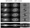 |
Fig. 1. Synthetic simulation images from Laurikainen & Salo (2017). In the left panels the direct image in the magnitude scale is shown, the middle panels show the contours of the same image, and the right panels show the unsharp mask image. In the four upper lines the galaxy inclination is fixed to i = 60°, whereas the azimuthal angle ϕ with respect to the bar major axis varies. In the lowest line the same model is seen edge-on. The initial values of the simulation contain a small classical bulge with bulge-to-total ratio B/T = 0.075. During the simulation a bar with a vertically thick inner barlens component forms. |
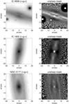 |
Fig. 2. Examples of the X-shaped bars. Left panels show the bar regions of the combined r′ + g′ + i′ SDSS mosaic images. Right panels show the unsharp mask images made for the r′-band mosaics, using the same image cuts. |
In this study the following nomenclature is used:
Photometric bulge: excess central light on top of the disk, extrapolated to the center.
Bar: elongated bar component (barlens flux not included).
Barlens (bl): a lens-like structure covering approximately one-half of barlength. It is assumed to be a vertically thick inner bar component (same as boxy/peanut/X).
Separate bulge component (or bulge): some galaxies have a central peak in the surface brightness profile (embedded in the barlens), which flux is fitted with a Sérsic function (see Sect. 5).
Central region (C): central galaxy region covering r = 0.3 × rbl (see Sect. 7.2). It is measured in a similar manner for all galaxies.
3. Sample selection
As a starting point we used the CALIFA survey of galaxies (Sánchez et al. 2012) described in detail by Walcher et al. (2014). This survey consists of galaxies in the mass range of M⋆/M⊙ = 109.7 − 1011.4, covering the redshift range z = 0.005 − 0.03. The CALIFA survey contains a mother sample of 939 galaxies, which are originally selected from Sloan Digital Sky Survey data release 7 (SDSS-DR7), and an extension sample of 125 galaxies, which are included in SDSS-DR12 (Alam et al. 2016). Altogether this makes 1064 galaxies. In the public data release DR2 (Sánchez et al. 2016a) IFU data cubes are given for 667 of these galaxies. From the sample of 1064 galaxies, and using the SDSS r′-band mosaic images (see Appendix A), we identified 236 galaxies that have either a barlens in the original image or an X-shaped feature in the unsharp mask image (see Sect. 4). Of these, 110 (+9 uncertain) have barlenses, and 124 (+3 uncertain) have X-shaped bars. In 15 additional galaxies both features were identified. Altogether this makes 24% of all CALIFA galaxies (excluding the uncertain cases). Taking into account the uncertain cases and the fact that we are probably missing some (∼7%) of the features because of an unfavorable viewing angle, we get 26% as an upper limit. Combining with the statistical uncertainty owing to the sample size indicates about 25 ± 2% frequency of Boxy/peanut/X/bl features.
The selected barlens and X-shaped galaxy samples are shown in Tables B.1 and C.1, respectively. The tables also show the redshifts, absolute r′-band magnitudes, and masses of the galaxies, as given in the public CALIFA data release (Sánchez et al. 2016a). As our intention in this study is to compare the photometric decomposition results with those derived using the IFU observations, not all barlens galaxies were decomposed. Instead, for the decomposition analysis a subsample of 54 galaxies was selected, including all barlens galaxies that have V1200 grating CALIFA data cubes available. Of these galaxies 6 had an uncertain barlens identification. Considering only the galaxies with clear barlens identifications, we were able to do reliable decompositions (with barlens fitted) for 46 of the 48 galaxies (shown in Table 1). The table also shows the Hubble stages from the CALIFA data release. We note that in NGC 6004 a barlens was identified, but because of its low surface brightness it could not be fitted. In NGC 7814 the bulge component has the size comparable to the image full width at half maximum (FWHM), which is the reason the effective radius is not given. Of the selected 54 galaxies V500 grating data cubes were available for 34 galaxies, of which 8 had uncertain barlens identifications. Excluding the uncertain cases, 26 galaxies were selected for stellar populations analysis. Of these galaxies 8 also have X features in the unsharp mask images. For all 26 galaxies reliable barlens decompositions were found. Our final samples are
- (1)
CALIFA sample of (N = 1064; unsharp masks).
- (2)
All barlenses (N = 110 + 9 uncertain).
- (2.1)
46 bl galaxies (new decompositions).
- (2.2)
26 bl galaxies (analysis of IFU data cubes).
- (2.1)
- (3)
All X-shaped galaxies (N = 124 + 3 uncertain).
Decomposed 46 barlens
4. Identification of structures and measuring the sizes of bars and barlenses
To identify the X-shape features unsharp mask images of the r′-band mosaic images were made for the complete CALIFA sample of 1064 galaxies. The way in which the mosaics were made is explained in Appendix A. To make the unsharp masks the images were convolved with a Gaussian kernel and the original images were divided by the convolved images. A few prototypical X-shaped galaxies were selected and used to find the optimal parameters for the Gaussian kernel. The galaxies were individually checked, and if needed, the convolution process was repeated many times with various kernel sizes and image contrast levels. Keeping in mind that the r′-band mosaics are strongly affected by dust obscuration particularly in the edge-on view, identification of the X-shaped feature was accepted even if it appeared only in one side of the galaxy. Some representative examples are shown in Fig. 21. Although barlenses were primarily identified visually in the original mosaic images, attention was also paid to the barlens morphologies in the unsharp mask images.
In this work the sizes and minor-to-major (b/a) axis ratios of barlenses were measured to be used as auxiliary data for making reliable structure decompositions. They were measured by fitting ellipses to the visually identified outer edges of barlenses in the original mosaic images, in a similar interactive manner as in Herrera-Endoqui et al. (2017). The barlens regions superimposed with the bar were excluded from the fit. From the fitted ellipses the major (a) and minor (b) axis lengths and position angles (PA) of the barlenses were measured. It was shown by Herrera-Endoqui et al. (2017) that this visual method is as good as if the outer isophotes of barlenses were followed instead. The measurements are shown in Table D.1. In the table barlengths are also given, which were visually estimated from the r′-band mosaic images by marking the bar ends in the deprojected images. The orientation parameters of the disks, estimated from the outer isophotes of the galaxies as in Salo et al. (2015), are also shown.
The galaxy inclinations of the complete CALIFA sample are shown in Fig. 3, plotted as a function of the absolute B-band galaxy magnitude. Different symbols are used to distinguish the barlens and X-shaped galaxies and the two subsamples of barlens galaxies (those with decompositions and those with IFU data). The 15 barlens galaxies with X-shape features are shown separately. It appears that the galaxies in our subsamples are fairly randomly distributed in magnitude, which means that they are representative examples of the complete CALIFA sample. The galaxies with barlenses and X-shaped features also have similar magnitude distributions. We note that, for consistency, in Fig. 3 values from HyperLEDA were used for all galaxies, including those for which we made our own measurements.
 |
Fig. 3. Galaxy inclination plotted as a function of the absolute B-band galaxy magnitude. The parameter values are from HyperLEDA. Gray dots indicate galaxies in the complete CALIFA sample of 1064 galaxies, green symbols show the X-shaped bars, red symbols the barlenses, and blue symbols the galaxies in which both features appeared. Filled red circles denote the barlens galaxies for which we made the decomposition, and open squares the 26 galaxies, for which the V500 grating SSP data cubes were also available. |
5. Multicomponent decompositions
5.1. Method and model functions
We used the GALFIT code (Peng et al. 2010) and the GALFIDL software (Salo et al. 2015) to decompose the 2D light distributions of the galaxies to various structure components. Our decomposition strategy is described in detail by Salo et al. (2015). The Levenberg-Marquardt algorithm is used to minimize the weighted residual χv2 between the observed and model images. The full model image consists of the models of the different structure components, each convolved with the image point spread function (PSF). The SDSS r′-band mosaic images, with the resolution of 0.396 arcsec/pix, were used. For each science frame a mask and a sigma-image mosaic were constructed. The σ image was used to control the weight of pixels in the decomposition. The PSF was made in such a manner that the extended tail beyond the Gaussian core was taken into account. The PSF FWHM = 0.8−1.4 arcsec, which agrees well with that obtained by MA2017. Preparation of the data for the decompositions is explained in more detail in Appendix A.
In GALFIT the isophotal shapes of the model components are defined with generalized ellipses (Athanassoula et al. 1990) as follows:
 (1)
The parameters x0, y0 define the center of the isophote, x′,y′ denote coordinates in a system aligned with the isophotal major axis pointing at the position angle PA, and q = b/a is the minor-to-major axis ratio. The shape parameter C = 0 for pure ellipses, for C > the isophote is boxy, and for C < 0 it is disky. Circular isophotes correspond to C = 0 and q = 1. The x-axis is along the apparent major axis of the component. The galaxy center is taken to be the same for all components. For the radial surface brightness distribution, the following Sérsic function was used for the bulges, barlenses, and disks:
(1)
The parameters x0, y0 define the center of the isophote, x′,y′ denote coordinates in a system aligned with the isophotal major axis pointing at the position angle PA, and q = b/a is the minor-to-major axis ratio. The shape parameter C = 0 for pure ellipses, for C > the isophote is boxy, and for C < 0 it is disky. Circular isophotes correspond to C = 0 and q = 1. The x-axis is along the apparent major axis of the component. The galaxy center is taken to be the same for all components. For the radial surface brightness distribution, the following Sérsic function was used for the bulges, barlenses, and disks:
![Mathematical equation: $$\begin{equation}\Sigma(r)= \Sigma_{\rm e} \exp \left(-\kappa \left[ (r/R_{\rm e})^{1/n} -1\right]\right), \end{equation}$$](/articles/aa/full_html/2018/10/aa33138-18/aa33138-18-eq2.gif) (2) where Σe is the surface brightness at the effective radius Re (isophotal radius encompassing half of the total flux of the component). The Sérsic index n describes the shape of the radial profile. The factor κ is a normalization constant determined by n. The value n = 4 corresponds to the R1/4 law, and n = 1 to an exponential function. For a bar a modified Ferrers function was used, i.e.,
(2) where Σe is the surface brightness at the effective radius Re (isophotal radius encompassing half of the total flux of the component). The Sérsic index n describes the shape of the radial profile. The factor κ is a normalization constant determined by n. The value n = 4 corresponds to the R1/4 law, and n = 1 to an exponential function. For a bar a modified Ferrers function was used, i.e.,
![Mathematical equation: $$\begin{equation} \Sigma(r)= \left\{\begin{array}{ll} \Sigma_o \left[1- (r/r_{\rm out})^{2-\beta}\right]^\alpha & r < r_{\rm out}\\ 0 & r \ge r_{\rm out}. \end{array} \right. \end{equation} $$](/articles/aa/full_html/2018/10/aa33138-18/aa33138-18-eq3.gif) (3) The outer edge of the profile is defined by rout, α defines the sharpness of the outer cut, and the parameter β defines the central slope. The parameter Σ° is the central surface brightness. When an unresolved component was identified in the galaxy center, it was fit with a PSF-convolved point source.
(3) The outer edge of the profile is defined by rout, α defines the sharpness of the outer cut, and the parameter β defines the central slope. The parameter Σ° is the central surface brightness. When an unresolved component was identified in the galaxy center, it was fit with a PSF-convolved point source.
5.2. Our fitting procedure
Our main goal is to extract barlenses from the other structure components. We started with single Sérsic fits to highlight possible low contrast features in the residual images, which were obtained by subtracting the model from the original image. Unsharp mask images were also useful to detect these features. Then bulge/disk (B/D) decompositions were made to find the initial estimate of the parameters of the disk, and also to have an approximation of the flux on top of the disk. In all of our decompositions the galaxy centers were fixed. Also the orientation parameters of the disk were fixed to those corresponding to the outer galaxy isophotes (see Table C.1). After the initial single Sérsic and B/D decompositions an iterative process was started in order to share the light above the disk between bars, barlenses, and possible separate bulge components (B/D/bar/bl models). Since the same function was used for the bulges and barlenses, we needed to carefully avoid possible degeneracy between the two components. Therefore, the starting values were selected to be as close to observation as possible. The parameters of the disk were kept fixed until good first approximations for all the other structure components were found. Once found, releasing the disk parameters in the fitting process typically did not change much the parameters of the other components. Only two galaxies in our sample have nuclear bars or rings visible in the direct images.
In order to avoid degeneracy between the structure components and also to reduce the number of free parameters in GALFIT, we utilized the measured sizes and shapes of bars and barlenses (see Sect. 4) when choosing the initial values in the decompositions. In practice, when using a Sérsic model for the barlens this means adjusting the Re so that the modeled barlens has similar outer isophote size as the visual estimate (a). In some cases, we had to fix the barlens Re. Moreover, their axial ratio was always fixed to the measured b/a ratio. Namely, the fact that the barlens flux is superimposed with that of the bar means that the barlens model, if completely free, can easily become artificially elongated along the bar major axis. Figure 6 shows the relation between the visually estimated size of the barlens and the size that comes out from our decompositions. A linear fit for galaxies where the barlens size was left as a free parameter indicates Re ≈ 0.36a. No large deviations from this trend are visible even in the cases where the barlens size was fixed.
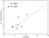 |
Fig. 6. Relation between the visually estimated barlens size (semimajor axis of the fitted ellipse) and the barlens effective radius that comes out in our decompositions. The dashed line shows the relation Re = 0.36a, which was obtained by a linear fit, to the values obtained in the decompositions in which barlens Re was a free parameter. The linear correlation coefficient between Re and a is 0.83. |
We followed an approach in which any of the parameters of the structure components could be temporarily fixed, until good starting parameters were found. For evaluating our best fitting model human supervision was important. In particular, we compared the observed and model images, the observed and fitted surface brightness profiles (1D and 2D), and the residual images after subtracting the model from the observed image.
5.3. Avoiding degeneracy between the fitted components
It is well known that in the structure decompositions the main source of uncertainty is the choice of the fitted components and possible degeneracy of the flux between those components, and not the formal errors given by the χ2 minimization2.
The most important factor is how many physically meaningful components are fitted, which is illustrated in Fig. 4. Shown are the B/D, B/D/bar, and B/D/bar/bl models for the galaxies NGC 7563 and NGC 5406. The B/D models for both galaxies fail to recover anything that could be designated as a real bulge. Including the bar improves the fit considerably, which agrees with many previous studies (Laurikainen et al. 2005, 2010; Gadotti 2008; Salo et al. 2015). How much the bar improves the fit depends on the surface brightness profile: for galaxies with small photometric bulges (NGC 5406) the B/D/bar model works very well, but if the photometric bulge is prominent and the profile is centrally peaked (NGC 7563), GALFIT tries to fit a massive bulge with a high Sérsic index. However, the B/D/bar/bl model for NGC 7563 fits the surface brightness profile more accurately. Most importantly, the model is consistent with what we see in the image. The galaxy outside the bar is not dominated by a large spheroidal, but rather by a dispersed ring with a down-bending surface brightness profile at the outer edge. The way in which the number of the fitted parameters affects B/T in the sample decomposed in this study is summarized in Fig. 5. An average B/T-value in the B/D-models is ∼0.30, in the B/D/bar models it is ∼0.15, and in the B/D/bar/bl-models ∼0.06.
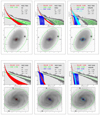 |
Fig. 4. Three decomposition models (B/D, B/D/bar, and B/D/bar/bl) shown for the galaxies NGC 7563 and NGC 5406. In the upper panels, the 2D representations of the surface brightness profiles are shown; black dots show the fluxes of the image pixels as a function of distance in the sky plane, and the white dots those of the total model images. The colors illustrate the fitted models of various structure components. Lower panels: r′-band mosaic images overplotted with the effective radii of the fitted models. |
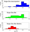 |
Fig. 5. Bulge-to-total (B/T) flux ratios for the 46 galaxies decomposed in this study. The values in three type of models are shown: bulge/disk (B/D, upper panel), bulge/disk/bar (B/D/bar, middle panel) and bulge/disk/bar/bl (B/D/bar/bl, lower panel). The B/T values for the individual galaxies are shown in Table 1. Compared to the B/D and B/D/bar models, the number of the B/D/bar/bl models is smaller because only half of the decomposed galaxies were fitted with a separate bulge component |
Our attempt to handle the bulge/barlens degeneracy was that two Sérsic functions were used only when two clear subsections with different slopes appear in the central surface brightness profile. The bar/barlens degeneracy is reduced using different fitting functions for the two components: Ferrers function for the bar and Sérsic function for the barlens. However, the bar/barlens separation worked well only if we did not fix the profile shape parameters of the bar (α and β) as is usually done. In the literature most bar decompositions have been carried out with fixed α ≥ 2 (e.g, see Salo et al. 2015; MA2017), whereas in the current study the final models typically adjusted α to values close to zero (on average α ∼ 0.15; for α close to zero the value of β has less significance; see Fig. 7). In our decompositions the bar is quite flat and sharply truncated at the outer edge. We further tested how much the small central light concentration introduced by a positive β value in Ferrers function can affect B/T. Changing β from 1.9 to 0 in the decomposition for NGC 7563 changes B/T only from 0.085 to 0.081 and in IC 1755 from 0.104 to 0.107, which means that the B/T using both β values are practically the same. Clearly, the large values of α used in earlier decompositions stem from the omission of the central barlens component.
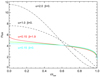 |
Fig. 7. Surface brightness profiles for the theoretical Ferrers function using different values for the parameters α and β, related to the sharpness of the outer truncation and the central slope of the profile, respectively. The lines indicate different combinations of α and β; the red line shows the typical values obtained in the current study. The different curves are normalized to correspond to the same total bar flux. |
5.4. Decompositions for a synthetic simulation image
Similar decompositions, such as those shown for the observed galaxies in Fig. 4, were also made for a simulation snapshot, taken from the N-body simulation model by Salo & Laurikainen (2017). These are stellar dynamical models with no gas or star formation carried out with Gadget-2 (Springel 2005) with self-consistent initial galaxy models. For the disk component, 5 × 10⁶ particles were used and to have good enough resolution a gravity softening ε = 0.01 hR was used, where hR is the scale length of the disk. The model mimics a typical Milky Way galaxy with a stellar mass of M⋆/M⊙ = 5 × 10¹⁰, a small preexisting bulge (B/T = 0.075, Re = 0.07 hR), an exponential disk, and a spherical halo. The decomposed snapshot (same as used in Fig. 1) was taken 3 Gyrs after the bar was formed and then stabilized. The model developed a vertically thick inner bar component, which is X shaped in edge-on view (see the lowest panel in Fig. 1), and a barlens morphology in more face-on view. During the simulation the bulge changed very little.
Our decompositions are shown in Fig. 8. It appears that the original bulge light fraction B/T is overestimated both in the B/D and B/D/bar decompositions (these yield B/T = 0.25 and B/T = 0.16, respectively), whereas the B/D/bar/bl decomposition recovers very well the small original bulge (B/T = 0.075) and the particles representing the barlens. The contribution of the bar is slightly overestimated in the B/D/bar model. The morphology and surface brightness profile of the simulated barlens galaxy is remarkably similar to those of the galaxies NGC 7563 and NGC 5406.
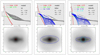 |
Fig. 8. Three decompositions (B/D, B/D/bar, and B/D/bar/bl) for a simulation snapshot taken from Salo & Laurikainen (2017). The model is explained in the text. The meaning of the lines and symbols are the same as in Fig. 4. |
Representative examples of the decompositions for the barlens galaxies are shown in Figs. 10, E.1a, and E.1b. The output decomposition files with the parameters of the different components of all the decomposed galaxies are shown in the web page3.
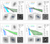 |
Fig. 10. Examples of our multicomponent decompositions. Large panel: black dots show the surface brightnesses (r′ magnitude/arcsec2) of the pixels in the two-dimensional image, white dots the values in the final model image, and the colors the values corresponding to the different structure components of the model. Bulges, disks, and barlenses were fitted with a Sérsic function, and bars with a Ferrers function. The decomposition parameters, galaxy masses (log M⋆), galaxy inclinations (i), and Hubble stages (T) are shown in the upper right. Lower panels (from left to right): region of the r′-band SDSS mosaic image, the same image with the model components plotted on top of that, and the unsharp mask image. The image in the large panel shows the full galaxy image. For more examples, see Appendix E. |
6. Comparison with MA2017
The galaxies that we decomposed have been previously decomposed by MA2017 using B/D/bar models. For comparison with their work we divided our decompositions into two groups: (a) galaxies in which the barlens had no clear central peak in the surface brightness profile, and (b) those in which a central peak appeared and were fitted with a separate Sérsic function. The mean parameter values are given in Table 2, where the values given by MA2017 are also shown. It is worth noticing that this division is to some extent artificial. This is the case because even those galaxies in which no separate bulge component was fitted might have some low luminosity central components, which possibly affects the Sérsic index.
We used group (a) to test the robustness of our decomposition method by comparing its results to MA2017. While we used GALFIT, MA2017 used GASP2D for their decompositions. Both codes use Levenberg-Marquardt algorithm to search for the model parameters. For non-exponential disks MA2017 used two truncated disks, while we used a Sérsic function with n < 1. In spite of these differences, our comparison shows that the B/D/bar decompositions in the two studies are in good agreement: both studies find the mean values of ⟨bl(bulge)/T⟩ = 0.13, ⟨n⟩ = 1.38, and ⟨Re⟩ = 0.60 − 0.64. This means that our method is robust: it is neither user dependent, nor is it sensitive to the code used or to the way in which the underlying non-exponential disk is fitted. However, our interpretation of the flux on top of the disk (after subtracting the bar) is different. We consider the central Sérsic component in the decompositions as a barlens, while MA2017 interpreted it as a separate bulge component.
For the galaxies in group (b), with both bulge and bl components in the decompositions, we found similar barlens parameters (bl/T = 0.13) as we also found for the galaxies in group (a). However, MA2017 find clearly higher values for the bulges, i.e., ⟨B/T ⟩ = 0.21 and ⟨n⟩ = 2.3. In our decompositions less than 10% of the total galaxy flux was left for a possible separate bulge component, which agrees with the previous study by Laurikainen et al. (2014) for barlens galaxies in the S4G+NIRS0S surveys. In both groups the surface brightness profiles of barlenses are nearly exponential; the mean values are ⟨n⟩ = 1.4 and 0.7 in the groups (a) and (b), respectively. The similarity of the barlenses in these two groups makes sense because their galaxies also have similar mean Hubble stages (⟨T⟩ = 2.1 ± 0.1 and ⟨T⟩ = 2.3 ± 0.1) and similar mean galaxy masses (log M⋆/M⊙ = 10.80 ± 0.04 and 10.69 ± 0.06 in groups (a) and (b), respectively). The similarity of the relative barlens fluxes in the two galaxy groups is illustrated in Fig. 9. The bl/T distributions are very similar once the contribution of the separate bulge component is taken away.
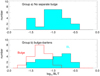 |
Fig. 9. Twenty-six barlens galaxies are divided into groups (a; upper panel) and (b; lower panel) as explained in Sect. 6. The blue histograms indicate the barlens flux fraction BL/T. Additionally, the red histogram (same as in Fig. 5, lowermost frame) in the lower frame shows the relative fluxes of the separate bulge components in the group (b) galaxies. |
The reason for the differences in our models and those obtained by MA2017 for the galaxies in group (b) can be understood by looking at individual galaxies. For NGC 7563 three decomposition models were shown in Fig. 4. It appears that the values B/T = 0.53 and n = 2.1 obtained by MA2017 are equivalent with those of our B/D/bar model with B/T = 0.54 and n = 2.4. However, in our final model B/T = 0.09 and bl/T = 0.31. In this galaxy the unsharp mask image clearly shows a barlens in favor of our model (see Fig. 10). Also, the surface brightness profile inside the bar radius is better fitted in our best model than in the more simple B/D/bar model. Other similar galaxies in our sample are NGC 5378 and NGC 7738. In NGC 5000 (see Fig. E.1a) the central mass concentration is less prominent, and therefore the difference in B/T between the two studies is also much smaller (B/T = 0.07 and 0.03 in MA2017 and our study, respectively). However, while MA2017 finds Sérsic n = 3.9 for this galaxy, we find n = 0.7. It is unlikely that this galaxy has a de Vaucouleurs’ type surface brightness profile because in the unsharp mask image X-shaped feature appears, which confirms the bar origin of the bulge. MA2017 also finds fairly large B/T and Sérsic n values for the galaxies NGC 0036 and NGC 1093, which are doubtful because these galaxies are late-type spirals with only a small amount of flux on top of the disk.
Mean parameter values of barlenses in group (a), and of barlenses and separate bulge components in group (b).
7. CALIFA data cubes and SDSS colors
7.1. CALIFA data cubes and SDSS colors
We used the CALIFA data cubes by Sánchez et al. (2016a) to obtain the stellar ages, metallicities, and velocity dispersions (σ) for the different structure components. For the average values of these parameters the SSP.cube.fits cubes were used, whereas to calculate the radial profiles of populations of different age and metallicity bins we used the SFH.cube.fits. The field of view (FOV) of the observations is 74″ × 64″, covering 2–3 Re of the galaxies. The FWHM = 2.5 arcsec corresponds to 1 kpc at the average distance of the galaxies in the CALIFA survey. CALIFA has two gratings, V500 and V1200, with the wavelength ranges of 2745–7500 Å with λ/Δλ = 850, and 3400–4750 Å with λ/Δλ = 1650, respectively. We used the V500 grating data-cubes, of which the pipeline data reductions are fully explained by Sánchez et al. (2016b). The spectral resolution is 327 km s−1. It was shown by Sanchez et al. that for the σ measurements there is a one-to-one relation between the two gratings when σ ≥ 40 km s−1. For the V1200 grating Falcón-Barroso et al. (2017) estimated 5% uncertainties for σ > 150 km s−1, 20% for σ = 40 km s−1, and 50% for σ = 20 km s−1. With the V500 grating this translates to uncertainties of 10% at σ > 150 km s−1, and 40% at σ = 40 km s−1. With the S/N ∼50 and having prominent stellar absorption lines, Falcón-Barroso et al. (2017) have reported that reliable σ values can be obtained down to 30 km s−1 within the innermost r ∼ 10″, without binning.
The pipeline (Pipe3D) reductions of the stellar populations and metallicities are explained by Sánchez et al. (2016b). Their spectral fitting included the following steps: First a simple Single Stellar Population (SSP) template is used to fit the stellar continuum, which is used to calculate the systemic velocity, central σ, and the dust attenuation. After that the emission lines were subtracted from the original spectrum and more sophisticated SSP templates were used to obtain stellar populations, metallicities, and star formation histories. The library covers 39 stellar ages (between 1 Myr and 13 Gyrs) and 4 metallicities in respect to solar metallicity (log10 Z/Z⊙ = −0.7, 0.4, 0.0 and 0.2). The templates used are a combination of the synthetic stellar spectra from the GRANADA library (Martins et al. 2005), and the libraries provided by the MILES project (Sánchez-Blázquez et al. 2006; Falcón-Barroso et al. 2011; Vazdekis et al. 2010). The Salpeter (Salpeter 1995) initial mass function was used. Sánchez et al. (2016b) estimated that with S/N ≥ 50 the stellar populations are well recovered within an error of ∼0.1 dex.
We also calculated the average (g′–r′) and (r′–i′) colors of the structure components using the SDSS mosaic images. As we are only interested in relative values between the structure components; no extinction corrections were made. The flux calibration parameters were taken from the image headers. The colors were calculated from the ratio of total fluxes in different bands, using the measurement regions described in the next subsection.
7.2. Definitions of the measured regions
Mean stellar ages and metallicities were calculated for different structure components of the galaxies, in the regions illustrated in Fig. 11, and defined in the following manner:
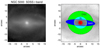 |
Fig. 11. Illustration of the measured galaxy regions, as defined in Sect. 7.2. Left panel: original r′-band mosaic image of NGC 5000 to show the bar region. Right panel: definitions of the regions. Red indicates galaxy center (C), turquoise indicates barlens (bl), blue indicate bar, and green indicates disk. |
C (galaxy center): an elliptical region around the galaxy center that has the same position angle and b/a axis ratio as the barlens, and an outer radius r = 0.3 rbl. This size is clearly larger than the maximum FWHM = 1.4 arcsec of the SDSS r′-band mosaic images, and larger than the FWHM = 2.5 arcsec of the V500 grating CALIFA data cubes. The radius was large enough to cover possible nuclear rings. This parameter is calculated for all galaxies, independent of whether a separate bulge component was fitted in the decomposition or not.
bl (barlens). an elliptical zone inside the barlens radius, but excluding the galaxy center C and the region overlapping with the bar. The b/a axis ratio and the position angle were those obtained from our visual tracing of barlenses (see Sect. 4).
bar (elongated bar). an elliptical region inside r = rbar, excluding the barlens. We used the measured position angle of the bar, and a fixed axial ratio b/a = 0.25.
disk (disk). an elliptical stripe between rbl and 2 rbl, excluding the zone covered by the bar. The ellipticity and position angle were the same as for the barlens.
Almost similar measurement regions were used in Herrera-Endoqui et al. (2017) for SDSS colors of the S4G-galaxies: in the current study “C” corresponds to what was denoted as “nuc2” in their study, and “bl” denoted as “blc” in Herrera-Endoqui et al.
8. Mean stellar populations, metallicities, and velocity dispersions
The mean stellar ages and metallicities of the structure components are shown in Table 3. The galaxies decomposed with (“bulge”) and without (“no bulge”) a separate bulge component are also shown separately (groups (a) and (b) in Sect. 6, respectively). Both mass (“m”) and light (“l”) weighted values are given. In the same table the mean stellar velocity dispersions σ, and the (g′-r′) and (r′-i′) colors are also shown. For these parameters the differences between barlenses and central galaxy regions (C-BL), and between barlenses and bars (BL-BAR) are illustrated in Fig. 12. The average values were obtained by finding all spaxels in the region of interest and calculating the density or luminosity weighted means of the corresponding (“m” and “l”, respectively) data cube values.
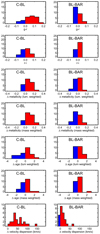 |
Fig. 12. Differences of the parameter values between the central galaxy regions and barlenses (C-BL), and between barlenses and bars (BL-BAR), are shown for the sample of 26 galaxies. Positive and negative deviations are shown with red and blue colors, respectively. The parameters are the same as in Table 3. |
The measurement regions inevitably correspond to a superposition of more than one structure component. In Fig. 13 we estimate the amount of contamination assisted by our decomposition models. The figure shows, for each measurement region, how much of the total flux in the decomposition comes from the structure we intend to measure. It appears that for the barlens measurement regions typically 20%–50% of the flux is due to the barlens; the rest is mainly due to the underlying disk. For the bar the disk contamination is slightly less; the contribution from the bar itself amounts to 30%–60%.
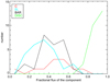 |
Fig. 13. Amount of contamination in the measurements of average values for different structure components from decomposition models from Sect. 5. The plot shows the distribution of the fractional contribution of the component itself to the total flux in the measurement region of that structure component, as defined in Sect. 7.2. |
8.1. Stellar velocity dispersions
Bars generally have old stellar populations, which means that prominent stellar absorption lines appear in the spectrum. The S/N in the bar region is also high because many spaxels are averaged. We find that bars and barlenses typically have fairly high velocity dispersions (σ = 130−160 km s−1), whose values are practically the same for both components (Δσ∼ 20 km s−1). Also, there is practically no difference in σ between bars and barlenses while comparing the galaxies with and without a separate bulge component. However, σ is clearly higher in the galaxy centers (σ = 207 ± 5 km s−1). Figure 12 shows that the central galaxy regions have always higher σ values than the surrounding galaxy components. The radial dependence of σ for the CALIFA sample has been shown by Falcón-Barroso et al. 2017.
8.2. Colors, stellar ages, and metallicities
We find that bars and barlenses have on average similar mean (g′-r′) and (r′-i′) colors, confirming the previous result by Herrera-Endoqui et al. (2017) for the S4G galaxies. The mean value (g′–r′)∼ 0.82 is typical for K-giant stars (Lenz et al. 1998). The central galaxy regions have clearly redder (g′–r′) colors (Δ (g′–r′)∼0.06), which is again in agreement with Herrera-Endoqui et al.. Most probably this is a dust effect because the stars in the central galaxy regions are also similar as in barlenses (light weighted average ages are 8.8 ± 0.2 and 8.7 ± 0.2 Gyrs, respectively).
The stellar ages in our analysis show gradients. The mass-weighted ages of the central regions are ∼0.5 Gyr, and the luminosity-weighted ages ∼1.6 Gyr older than for the disks. These gradients are in a qualitative agreement with those obtained for the whole CALIFA sample, by García-Benito et al. (2017) for the mass-weighted ages, and by González Delgado et al. (2014) for the luminosity-weighted ages. It is remarkable that despite these age gradients, the ages of bars and barlenses, which appear at different radial distances in our measurements, are similar. Their mass-weighted mean ages are ∼9 Gyrs and the luminosity-weighted mean ages ∼5 Gyrs.
We also show a metallicity gradient of log10 Z/Z⊙ ∼0.1 (using both mass and light weighted values) in a sense that the disks are less metal rich than the bars and barlenses. The galaxy centers are more metal rich than the rest of the galaxy, both using the mass and luminosity-weighted indices. These gradients are again in a good qualitative agreement with those obtained by González Delgado et al. (2015) for the whole CALIFA survey. Like the ages, the metallicities are similar for bars and barlenses; their mean luminosity-weighted values are log10 Z/Z⊙ = − 0.09 ± 0.02 and −0.10 ± 0.02, respectively.
Figure 12 illustrates the similarity of all the measured parameter values of bars and barlenses, and also the way in which the central galaxy regions in many parameters are at least marginally different from bars and barlenses.
Mean parameter values calculated for the different structure components using the CALIFA V500 data cubes (e.g., Sánchez et al. 2016a).
9. Radial profiles of stellar ages and metallicities
We used the CALIFA SFH cubes to analyze the radial distribution of different age and metallicity populations. For the analysis we selected typical barlens galaxies, galaxies with dust lanes, and barlens galaxies in which X-shaped features also appear. The age and metallicity profiles are shown in Figs. 14, E.2a, and E.2b. The decompositions for the same galaxies were shown in Figs. 10, E.1a, and E.1b. The profiles are azimuthally averaged in a few arcsecond bins after deprojecting the galaxies to face-on. This means that in the barlens regions and galaxy centers the stellar parameters are well captured, but the bar regions might be slightly contaminated by younger stellar populations of the disks. The four metallicity bins are as given in the CALIFA data cubes (SFH.cube.fits). The original stellar age bins were rebinned into three bins corresponding to young (age < 1.5 Gyr), intermediate age (1.5 < age < 10 Gyrs), and old (age >10 Gyrs) stars. According to the headers of SFH.cube.fits files, the spaxel values of the SFH data cubes correspond to luminosity fractions of different age and metallicity bins. Our comparisons indicated that the mean ages and metallicities calculated from the SFH cube distributions are close to the mean of metallicity and luminosity averaged mean ages and metallicities, as given in the SSP cubes.
9.1. Typical barlens galaxies
NGC 7563 (T = 1). This is the type of galaxy in which barlenses were originally recognized (Laurikainen et al. 2011). The surface brightness profile (Fig. 10) shows a possible separate bulge component, and a nearly exponential barlens that dominates the photometric bulge. The bar and barlens are dominated by metal-rich (log10 Z/Z⊙ = 0.20) intermediate age stars. There is also a contribution of very old stars (>10 Gyrs), but their relative fraction decreases within the barlens and drops in the galaxy center. The bar is surrounded by a dispersed ringlens, which is also dominated by metal-rich stars, but also contains an increasing fraction of less metal-rich stars. It appears that the density peak in the surface brightness profile is not made of old metal-poor stars early in the history of this galaxy.
NGC 5406 (T = 3.5). The distributions of the oldest and intermediate age stars in the bar/barlens regions are similar to NGC 7563, i.e., the fraction of the oldest stars drops at the galaxy center compared to the barlens region. Outside the barlens the fraction of younger stars increases owing to the prominent spiral arms. However, the disk is dominated by very metal-poor stars (log10 Z/Z⊙ = −0.7), whose fraction starts to drop in the bar region so that in the galaxy center those stars have disappeared. Therefore, in this galaxy as well the bar and barlens have had repeated episodes of stars formation that have enriched the gas in metals. In the disk outside the bar that has happened to a lesser extent than in NGC 7563. The galaxy center has a higher velocity dispersion (σ = 214 km s−1) than the bar or barlens (σ = 128 and 142 km s−1, respectively), most probably related to higher stellar density.
NGC 7321 (T = 3). This galaxy has qualitatively similar stellar age and metallicity distributions as NGC 5406, but the photometric bulge is less prominent. The fraction of the most metal-poor stars (log10 Z/Z⊙ = −0.7) starts to drop at r ∼18″ already, corresponding to the high surface brightness region extending well outside the bar. There is clearly migration of stars inside the high surface brightness disk.
UGC 10811 (T = 2). This galaxy (and NGC 0180) is exceptional in our sample in the sense that the barlens is dominated by the oldest (>10 Gyrs) fairly metal-poor (log10 Z/Z⊙ = −0.40) stars, whose fraction increases toward the galaxy center. The photometric bulge is dominated by the barlens, which has a nearly exponential surface brightness profile (n = 1.5). The disk outside the bar is dominated by young metal-rich stars (log10 Z/Z⊙ = 0.20), but also has many other metallicities. Most probably the bar was formed early, but galaxy modeling is needed to interpret how the mass was accumulated to the barlens.
NGC 0776 (T = 3). The barlens dominates the bar in such a level that the morphology approaches a non-barred galaxy (i.e., has a barlens classification “f” by Laurikainen & Salo 2017). However, in spite of that the stellar and metallicity properties are very similar as in such prototypical barlens galaxies as NGC 5406. The unsharp mask image shows a nuclear ring, also showing a significant contribution of the young stellar population.
9.2. Galaxies with X-shapes
NGC 6941 (T = 3), UGC 8781 (T = 3), and NGC 5000 (T = 4). In these galaxies the barlenses also show X-shaped features in the unsharp mask images, which confirms that they are vertically thick inner bar components. Therefore, it is interesting that in these galaxies the bar/barlens regions have similar age and metallicity distributions as the prototypical barlens galaxies discussed above, i.e., they are dominated by metal-rich (log10 Z/Z⊙ = 0.20) intermediate age stars with a significant contribution of the oldest stars (age > 10 Gyrs). In UGC 08781 and NGC 5000 the fraction of the oldest stars is similar in the galaxy center and in the bar/barlens region, whereas in NGC 6941 their fraction drops in the galaxy center. In these galaxies the metallicity starts to drop toward the galaxy center already at the edge of the bar.
NGC 0180 (T = 3). The bl/X is dominated by old (age > 10 Gyrs) metal-poor (log10 Z/Z⊙ = −0.40) stars, in a similar manner as the barlens in UGC 10811. In the galaxy center the fraction of the oldest stars drops. The mean velocity dispersions of the bar, bl/X, and the galaxy center are σ = 118, 137, and 181~km s−1, respectively. Very old metal-poor stars with high random motions are generally interpreted as manifestations of merger built classical bulges. However, in NGC 0180 the barlens is dominated by an X-shaped feature, which challenges that interpretation.
9.3. Barlenses with dust lanes
NGC 7738 (T = 3). This is a prototypical barlens galaxy, similar to NGC 4314 (Laurikainen et al. 2014). The arc-like dust features in the unsharp mask image are illustrative because they hint at the fact that the whole high surface brightness disk surrounding the bar probably forms part of the bar structure. Two dust lanes penetrate through the barlens ending up at the galaxy center, where young stars (age < 1.5 Gyr) appear at r ∼ 5 arcsec. This galaxy is enriched in metallicity particularly in the barlens region. Clearly, fresh gas has penetrated through the barlens fairly recently triggering central star formation. Most probably star formation has also occurred in the barlens, leaving behind a metal-rich stellar population, but that star formation has already ceased a long time ago (lack of young stars in the barlens).
NGC 5378 (T = 3). Two dust lanes appear: one lane penetrates through the barlens ending up at the galaxy center, and another weaker lane follows the outer edge of the barlens. As in NGC 7738, in this galaxy particularly the barlens and bar are places of metallicity enrichment.
NGC 0171 (T = 3). This is a barlens galaxy seen nearly face-on. The unsharp mask image shows an elongated feature along the bar major axis at low surface brightness levels. A nuclear ring is manifested as an obscuration by dust. The metal enrichment has occurred particularly at the edges of the bar and barlens. However, contrary to the other barlens galaxies the fraction of the metal-poor stars (log10 Z/Z⊙ = −0.70) starts to drop at r ∼24 arcsec already, where the two-armed prominent spiral arms start. It seems that mixing of different stellar ages and metallicities appear in a large galaxy region, starting well outside the bar via the prominent spiral arms.
10. Cumulative age and metallicity distributions
Above we have discussed the mean stellar ages and metallicities and looked at their radial distributions in individual galaxies. In order to make a more clear comparison between the structure components, cumulative distributions of the mean stellar ages and metallicities were derived and are shown in Fig. 15. Both luminosity and mass-weighted distributions are shown. While constructing these distributions, we used the measurements in the zones as defined in Fig. 11.
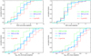 |
Fig. 15. Cumulative distributions of the average ages and metallicities in the different structure components, measured in regions as defined in Fig. 11. Included are the 26 barlens galaxies in our sample. The V500 data cubes by Sánchez et al. (2016a) (SSP.cube.fits) were used, loaded from the CALIFA database. Distributions are based on median values of the pixels covered by the structure components; practically identical distributions are obtained when using flux-weighted means. Labels indicate the p-values in KS-tests comparing the distribution with that of barlenses; p < 0.05 indicates a statistically significant difference. |
It appears that bars and barlenses have remarkably similar age and metallicity distribution. The luminosity-weighted mean stellar ages are typically 4–8 Gyrs, and the mass-weighted indices show stars older than 8 Gyrs (with a few exceptions). Using the mass-weighted indices, the oldest stars in barlenses are as old as the oldest stars in the galaxy centers (∼11 Gyrs), which are not much older than those in bars (i.e., ∼10 Gyrs). The metallicities are near solar, but vary from slightly subsolar (log10 Z/Z⊙ = −0.3) to slightly supersolar metallicities (log10 Z/Z⊙ = 0.1). In some galaxies the central regions are dominated by younger stars of 3–6 Gyrs, which can be explained by more recent star formation in possible nuclear rings, which are not well resolved in the used data cubes. The disks within the bar radius have typical luminosity-weighted stellar ages of 3–6 Gyrs, and the oldest stars are ∼9 Gyrs old. The disks are on average more metal poor than the bars and barlenses, whereas the central galaxy regions are more metal rich.
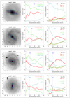 |
Fig. 14. Left: deprojected SDSS r′-band mosaic image. Overplotted are the elliptical zones (see Sect. 7.2) used in the measurement of structure averages shown deprojected to the disk plane (original measurements were carried out in non-deprojected images). Middle: Fractions of stars in the three stellar age bins, as a function of the deprojected radial distance. The profiles are constructed using the V500 grating data cubes from Sánchez et al. (2016b), loaded from CALIFA database (SFH.cube.fits). These profiles correspond to averages over mass and luminosity-weighted star formation histories. The vertical lines show the deprojected semimajor axis lengths of the bars, barlenses, and the central galaxy regions. Right: fractions of stars in four different metallicity bins, as given in the CALIFA data cubes. The meaning of the vertical lines are the same as in the middle panel. For more examples, see Appendix E. |
The KS tests find no significant differences between the age and metallicity distributions of bars and barlenses. Judging by eye the center regions and barlenses seem to deviate more. However according to the KS test, their differences are not statistically significant. On other hand, the disks have clearly different luminosity-weighted stellar age and metallicity distributions than barlenses: p = 0.031 and 0.002, respectively, although the difference is no more statistically significant when the distributions from mass-weighted indices are compared. It is worth keeping in mind that our number of galaxies is fairly small for these kinds of statistical tests; also the overlap of flux between various components tends to dilute possible underlying differences.
In summary, based on our analysis the stellar age and metallicity distributions of bars and barlenses are very similar, and therefore barlenses must have been formed in tandem with bars. Barlenses have a range of stellar ages and metallicities, which means that their masses must have been accumulated in several episodes of star formation. An important fraction of those stars were formed early in the history of the galaxy.
11. Discussion
In the previous sections we have analyzed the photometric bulges, i.e., the excess mass and flux on top of extrapolated disk profile. In which way this mass has accumulated in galaxies is an important question in cosmological models of galaxy formation and evolution. The photometric bulge can consist of a classical bulge, which is a spheroidal formed in non-dissipative processes (but see also Falcon-Barroso et al. 2018; Hopkins et al. 2009), a disky pseudo-bulge (or simply a pseudo-bulge), which is a small dissipatively formed inner disk, or it can be a boxy/peanut/bl structure, related to the inner orbital structure of bars. If the classical bulge is small all types of structures can form part of the same photometric bulge. Not only the boxy/peanut/bl, but also the elongated bar can comprise an important part of the photometric bulge. Only the classical bulges are real separate bulge components that are not related to the evolution of the disk.
However, distinguishing the origin of the photometric bulges has turned out to be complicated. Depending on which emphasis is given to each analysis method different answers are obtained, and in particular not much has been done to investigate how the boxy/peanut/bl bulges should appear in the different analysis methods. As examples of such controversial results three recent papers are discussed below. All papers used mostly CALIFA IFU observations for kinematics, and in the structure decompositions the bar flux, if present, is taken away from the photometric bulge.
11.1. Interpretation of photometric bulges in three recent studies
Neumann et al. (2017) studied 45 non-barred galaxies with a large range of Hubble types. Their conclusion was that using the Kormendy relation (log10 Re vs. μe) and the concentration index (C20,50), pseudo-bulges can be distinguished from classical bulges with 95% confidence level. In the Kormendy relation these bulges appeared as outliers toward lower surface brightnesses. Other parameters such as B/T, Sérsic n, and the central σ profile appeared as expected for the two type of bulges. They found that even 60% of the bulges in their sample were classical bulges.
Costantin et al. (2017) studied 9 low mass late-type spirals. In spite of the low galaxy masses, the bulges of these galaxies followed the same fundamental plane and the Faber–Jackson relation as the bulges of bright galaxies. In the Kormendy relation these bulges appeared as low surface brightness outliers as expected for their low galaxy masses. For these similarities in the photometric scaling relations, Costantin et al. concluded that there is only a single population of bulges that cannot be disk-like systems, i.e., all bulges are classical.
Méndez-Abreu et al. (2018) studied 28 massive S0s, but did not find any correlation between the photometric (B/T, Sérsic n) and kinematic (the angular momentum λ parameter, and Vrot/σ) parameters of the bulges. They reached the conclusion that perhaps all bulges were formed dissipatively. For massive S0s this already happened at high redshift, for example, after major mergers. The authors reached the opinion that identification of bulges photometrically is not meaningful at all.
How do we understand these controversial results? It appears that in the sample by Neumann et al. (2017) a large majority of the galaxies they classified as having pseudo-bulges have Sc–Scd Hubble types (i.e., have low galaxy masses), and a similar fraction of their classical bulges have S0–Sb types (i.e., have high galaxy masses). Having in mind that the Kormendy relation strongly depends on galaxy mass (Ravikumar et al. 2006; Costantin et al. 2017), the low surface brightness outliers in the Kormendy relation, interpreted as pseudo-bulges by Neuman, Wisotzki, and Choudhury, have a natural explanation, which is reflected also in the concentration parameter C20,50: i.e., bulges in low mass galaxies often have disk-like properties (e.g., Fisher & Drory 2008, 2016). It is worth noticing that the bulges of the low mass galaxies in their study also have other indices of pseudo-bulges, i.e., recent star formation or spiral arms penetrating into the central galaxy regions. In the study by Costantin et al. only the scaling relations were used to distinguish the type of bulges. However, the bulges of the low mass galaxies in their study, interpreted as classical bulges, have recent star formation or spiral arms penetrating into the central galaxy regions, which are actually characteristics of disk-like pseudo-bulges.
Méndez-Abreu et al. (2018) made Schwarzschild models, which are able to build up galaxies by weighting the stellar orbits using the observed gravitational potential derived from observation. This makes it possible to calculate the kinematic parameters as in real galaxies, look at the galaxies at different viewing angles, and approximate possible disk contamination on the bulge parameters. That they did not find any correlation between the photometric and kinematic parameters of bulges is interesting because bright S0s are known to have the most massive bulges in the nearby universe. We come back to this question in the next section.
In conclusion, it seems that the bulges identified as disky pseudo-bulges in the Kormendy relation are generally low mass galaxies that can be recognized as such also via specific morphological, photometric, or star formation properties. However, lacking these indicators does not necessarily mean that the bulges are classical, not even in case when they follow the same scaling relations (Kormendy, Faber–Jackson, fundamental plane) as bright ellipticals. The scaling relations were introduced to describe virialized systems such as elliptical galaxies. Fast rotating systems can also have fairly large velocity dispersions, and it is not well studied what kind of deviations from the scaling relations of ellipticals are expected for such structures as the boxy/peanut/bl components.
11.2. Nature of barlenses in the CALIFA survey
In the current study a different approach was taken. We first identified all the vertically thick inner bar components (boxy/peanut/X/bl) in the CALIFA survey, then made detailed B/D/bar/bl decompositions for 48 barlens galaxies (out of which 46 were considered reliable), and in a half of these also studied the stellar populations and metallicities of the different structure components.
A number histogram of the minor-to-major (b/a) axis ratios of the CALIFA galaxies is shown in Fig. 16, and on top of that histograms of the galaxies with barlenses and X-shape features are also shown. As expected, the X-shaped galaxies reside preferably in highly inclined galaxies and the barlenses in more face-on systems and there is a significant overlap between the two. An important fact is that the combined distribution of barlenses and X-shapes forms a very similar histogram as obtained for the complete CALIFA sample. As the fraction of the vertically thick inner bar components should not depend on galaxy orientation, the distributions are consistent with the interpretation that barlenses and X-shaped features are manifestations of the same structure seen at different viewing angles. The same conclusion for the S4G+NIRS0S galaxies (z < 0.01) was previously made by Laurikainen et al. (2014). Taking into account that in 5–10% of the cases the geometry is not favorable for distinguishing such components, and assuming that half of the galaxies are barred, ∼50% of the barred galaxies in CALIFA are estimated to have vertically thick inner bar components. This is practically the same percentage as the 46% found by Laurikainen et al. (2014) for the S4G+NIRS0S galaxies. The number is also consistent with that obtained by Li et al. (2018) who found that 38% of barred galaxies with inclinations i < 70° in the Carnegie-Irvine Galaxy Survey, have either a barlens or a boxy/peanut. The galaxies they studied are at similar distances and have similar host galaxy masses as those in S4G+NIRS0S.
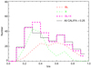 |
Fig. 16. Distributions of the minor-to-major (b/a) axis ratios of the galaxies hosting barlenses (bl; our sample 2) and X-shaped features (X; our sample 3) in the CALIFA sample. The combined bl+X distribution is compared with that of the complete sample of CALIFA galaxies (our sample 1), scaled by a factor of 0.25. The histograms for both bl and X include the 15 galaxies in which both features appear. In the combined bl+X histogram these galaxies are included only once. The b/a values are from our measurements when available, otherwise from HyperLEDA. However, use of HyperLEDA inclinations would yield very similar distributions. |
Nearly 60% (16/28) of the kinematic sample of Méndez-Abreu et al. (2018) form part of our sample of barlens galaxies, ten of which we decomposed. In their study the B/D/bar decompositions from MA2017 were used. All the bulges in Méndez-Abreu et al. (2018) followed the same Kormendy relation as the bright elliptical galaxies (see their Fig. 8), including the 16 barlens galaxies. However, if we use the (V/σ)−ϵ plane diagnostics4, using the kinematic parameters of bulges within 1 Re, given by Méndez-Abreu et al. (2018), the 16 barlens galaxies fall above the bright elliptical galaxies. These galaxies are typically slowly rotating systems (see Fig. 17) which have lost their opportunity to become fast rotating systems anymore because they are heated systems (see Emsellem et al. 2011). Barlenses appear in the same region with the fast rotating ellipticals, which adds one more complexity for the interpretation of this diagram, i.e., the vertically thick inner bar components (barlenses) can have similar kinematic properties as those classical bulges formed by wet major or minor mergers (see Naab et al. 2014). This diagram also shows that barlenses are not oblate systems as expected in case of disky pseudo-bulges (Pfenniger & Norman 1990; Friedli & Benz 1995).
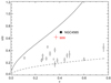 |
Fig. 17. Sixteen barlens galaxies common with Méndez-Abreu et al. (2018) and this work are shown in the V/σ−ϵ plane. The parameters refer to values measured within one Re of the bulge (see Table 2 in Méndez-Abreu et al. 2018). They are corrected for pixelation and resolution effect (as explained in the original paper). The solid line shows the expected relation for rotationally flattened oblate spheroids seen edge-on, following the approximation |
A novelty of our study is to make a hypothesis that the photometric bulges in the barred CALIFA galaxies are largely dominated by barlenses, of which clear examples with identified barlenses were studied. Although our starting point was morphological, the studied physical parameters are also found to be consistent with this picture. Taking this view, the inconsistencies in the literature, using the different analysis methods applied to barlens galaxies, become more understandable. We find that not only the (g′–r′) and (r′–i′) colors, but particularly the cumulative distributions of stellar ages and metallicities are very similar in bars and barlenses. The stars in barlenses accumulated over a large time period in several episodes of star formation, manifested in a range of stellar ages of (4–11 Gyrs) and metallicities. It seems that barlenses gradually increased in mass in tandem with the rest of the bar. The bar origin of the barlens further confirmed for a few galaxies showing X-shape features in the unsharp mask images. The mass-weighted stellar ages of barlenses are also similar as those obtained by Pérez et al. (2017) for the X-shaped bar in NGC 6032 (mean age ≥ 6 Gyrs). Prominent dust lanes in some of the barlens galaxies in our sample show how gas can penetrate through the barlens possibly triggering star formation in the galaxy center and at some level also in the barlens itself. The relative fluxes of barlenses (bl/T) in our decompositions do not correlate with the stellar velocity dispersions measured in the same galaxy regions (see Fig. 18).
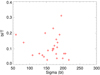 |
Fig. 18. Relative flux of barlens (bl/T) as a function of velocity dispersion σ of the same component. The barlenses in our subsample of 26 galaxies are plotted. |
Our finding that the old and intermediate age stars dominate bars and barlenses is consistent with the kinematic analysis of the C ALIFA survey by Zhu et al. (2018). The kinematic decompositions by Zhu et al. uses the parameter λz (orbit angular mom entum relative to circular orbit with the same energy) as a dividing line. The orbits in their study are defined as cold when λz > 0.8, hot when λz < 0.1, and warm in between these two λz values. In their study the photometrically identified bulges (flux on top of the disk) are dominated both by hot and warm orbits, corresponding to our old and intermediate age stars. The bulges are only dominated by hot orbits in the most massive galaxies with M⋆ > 1011 (not included in our sample).
If photometric bulges in Milky Way mass disk galaxies were dominated by bars and barlenses there is no reason why they should appear in the same location as elliptical galaxies in the V/σ − ϵ plane. Neither should they behave in a similar manner as star forming pseudo-bulges in the disk plane. Barlenses can be dynamically hot, have fairly high effective surface brightnesses (μe) for given effective radii (Re), and also have fairly old stellar populations, which in some analysis methods can mislead the interpretation of their origin.
11.3. Comparison with the Milky Way bulge
The Milky Way (MW) bulge is known to have strong evidence for being of bar origin. The bulge is X-shaped and cylindrically rotating, as detected in the distribution of the red clump giant stars (Wegg & Gerhard 2013; Ness & Lang 2016). From our point of view it is important that the MW bulge can also be considered a barlens. In face-on view the bulge has been suggested to have a similar morphology as the barlens in NGC 4314, which is a galaxy seen nearly face-on (see the review by Bland-Hawthorn & Gerhard 2016). In CALIFA, for example NGC 7563 has a similar galaxy/barlens morphology.
The MW bulge is dominated by old red clump giant stars (McWilliam & Rich 1994; Zoccali et al. 2008), but has also stars with intermediate ages (Clarkson et al. 2011; Bensby et al. 2011), which is qualitatively in agreement with what we see also in barlenses. The main body of the stars have slightly subsolar metallicities and ages between 9 and 13 Gyrs, and a small contribution of stars younger than 5 Gyrs. The X feature in the MW bulge has been detected in the distribution of the red clump stars (MacWilliam & Zoccali 2010; Nataf et al. 2010; Wegg & Gerhard 2013; Ness & Lang 2016), but not in that of the very old RR Lyrae stars (e.g., Wegg & Gerhard 2013), which has provoked a discussion of a possible additional classical bulge in the MW. The MW bulge has also a nuclear disk at r < 200 pc, showing recent star formation (Launhardt et al. 2002). Nuclear disks with stellar ages of <4 Gyrs also appear in some of the barlens galaxies in our sample. In fact, many barlenses in the local universe have embedded star forming nuclear rings or disks (Laurikainen et al. 2011). However, in CALIFA sample the resolution is not ideal for detecting those.
In the MW bulge high-metallicity (HM) stars are concentrated in the X feature and close to the Galactic plane (Zoccali et al. 2008; González et al. 2013; Johnson et al. 2011), whereas the low-metallicity (LM) RR Lyrae stars form a more round component (Dékány et al. 2013), which is also centrally peaked (Pietrukowicz et al. 2015). Together the LM and HM stars make the observed metallicity gradient, so that the metallicity decreases toward higher galactic latitudes. For barlenses we do not have information about the vertical metallicity distributions, but as we are looking at the galaxies in fairly face-on view, most probably we see a superposition of both components manifested as a large range of stellar metallicities. Both in the MW bulge and in the barlenses the oldest metal-poor stars form a minority in their stellar populations. As shown in Fig. 17, in the V/σ−ϵ plane the MW bulge appears slightly below the oblate line, and is clearly above the bright elliptical galaxies (Rich et al. 2008; Minniti & Zoccali 2008). In fact, this is what we also see for barlenses in our sample. It is interesting that in that diagram the MW bulge, seen almost end-on (ϕ = 27°; Wegg & Gerhard 2013), appears almost in the same location with NGC 4565, which is considered as a twin of the MW; NGC 4565 is seen nearly end-on and has an X-shaped bulge (Kormendy et al. 2010; Laurikainen et al. 2014).
11.4. Explaining the boxy/peanut/X/bl structures
The backbone of the vertically thick inner bar components consist of both stable periodic orbits and unstable periodic orbits linked to chaos (see the review by Athanassoula 2016). It has been suggested (Abbott et al. 2017; Wegg & Gerhard 2013; Portail et al. 2015) that the boxy/X-shaped bulge of the MW consists of a superposition of various types of bar orbits, a majority of which are non-resonant box orbits (constituting 60% of bar orbits). Only the banana-type X1 and the resonant boxlet (i.e., fish/brezel) orbits make the X-shaped feature. Most probably barlenses are a superposition of similar orbital families. In the simulation models the X features are like horns that are extended both in xy and xz-directions (Athanassoula et al. 2015; Salo & Laurikainen 2017). When the galaxy inclination decreases the banana-type orbits, which are visible in edge-on view, gradually become overshadowed by the more circular or chaotic orbits possibly making the barlens appearance. In the overall morphology this is shown with the simulation models by Salo & Laurikainen (2017), and is also manifested in the CALIFA sample as a gradual changing of the X-shaped features into barlenses toward lower galaxy inclinations (Fig. 16). If the fraction of the central concentration is not high enough or even if the resolution in the simulation models is insufficient, for example, because of large gravity softening, the vertically thick inner bar component is centrally pinched at all galaxy inclinations (Salo & Laurikainen 2017). Such pinched structures in face-on view are also shown in the simulation models by Saha et al. (2018). However, in observations such pinched structures in nearly face-on view are rare.
In the interpretation of the MW bulge a critical point has been to explain why the fairly round component with old metal-poor RR Lyrae stars exists and what causes the vertical metallicity gradient. Depending on the model, either a small or no classical bulge has been suggested, superimposed with the boxy bulge. In the simulation models of Shen et al. (2010) the relative flux of the classical bulge is 8–10% at most, which is consistent with that we obtained in the barlens galaxies: i.e., ≤10% of the total galaxy flux appears in a component, which could be interpreted as a possible classical bulge.
Detailed models for the MW bulge have shown that it is possible to explain, not only the X-feature, but also the more round LM component without invoking the concept of a classical bulge. Pérez-Villegas et al. (2017) explained the old metal-poor population of the MW bulge as an inward extension of the slowly rotating metal-poor stellar halo. The mix of stars in their N-body models is due to the gravitational interaction between the bar and the boxy/peanut when they form and evolve. In the chemo-dynamical models by Athanassoula et al. (2017) the MW bulge morphology is coupled with the kinematics, metallicity, and stellar ages. The different metallicity bins have specific velocity dispersions and different locations in the bulge. The LM population makes the more round component including the thick disk, stellar halo, and a possible small classical bulge, whereas the HM population contributes only to the X feature. The coupling of stellar ages and metallicity with the kinematics and morphology in the MW bulge has been discussed in detail by Portail et al. (2015).
It seems that although detailed information of the stellar populations of the MW bulge is available, it has not been possible to show unambiguously that there also exists a small classical bulge embedded in the boxy bulge. At some level we have the same concerns regarding our analysis of barlenses in this study. In half of the studied galaxies separate bulge components were fitted, whose components are potential small classical bulges. However, instead of being dominated by the oldest stars (>10 Gyrs) as expected for merger built structures, in many barlens galaxies the fraction of the oldest stars even drops in the galaxy center. The most prominent barlenses in the simulation models form in centrally peaked galaxies (Salo & Laurikainen 2017), but the question remains about whether the central mass concentration or barlens forms first. Also, in half of the barred MW mass galaxies in the CALIFA sample no vertically thick inner bar components were identified. It needs to be further investigated in which physical conditions they form in galaxies. An interesting observation pointed out in this study was a drop of the most metal-poor stars, both in the galaxy center and barlens region, and in some galaxies in the elongated bar as well. In the simulation models by Pérez et al. (2017) some migration of stars occurred within the boxy/peanut, but the stars formed in the galaxy center and in the outer part of the bar stayed in their original locations.
11.5. Bars in the context of galaxy formation and evolution
It has been shown by Scannapieco & Athanassoula (2012) that realistic bars can form in hydrodynamical cosmological simulations. The disk and even the dark matter halo keep growing while the bar forms. They reran one of their simulations with higher resolution using the Tree-PM SPH code, including star formation and chemical enrichment. The model ended up forming bars that have morphologies, sizes, and surface brightness profiles similar to those observed at z = 0. Athanassoula et al. (2017) studied the bar/bulge regions of galaxies starting from merging proto-galaxies composed only of dark matter and gas. In their models, the stars that ended up as bulge and halo stars formed in a short time period (1.4 Gyr) before the galaxy merger. The stars born during the merger at high redshift contributed to a thick disk and a spheroid, whereas the gas accreted from the halo formed a thin disk, including the bar and boxy/peanut bulge. So, based on these models the stellar populations of the classical bulges are expected to have clearly older stellar populations than the boxy/peanut/bl bulges.
The galactic halos can interact with the environment and therefore continuously evolve. Although a small fraction of stars in the halos might be accreted as small satellites, most of the halo stars were formed in starbursts, which stars are ∼1 Gyr younger, have higher metallicities, and are less α-enhanced than the accreted stars (Tissera et al. 2018). According to the simulation models (Hirschmann et al. 2013; Hopkins et al. 2014; Stinson et al. 2013; Woods et al. 2014) gas accretion to the disk is decoupled from the halo assembly, which allows continuous gas accretion keeping the star formation rate in the disk constant (Christensen et al. 2016; Oppenheimer et al. 2010; Ubler et al. 2014). As a consequence, the structures formed of disk stars are expected to have a large range of stellar ages and metallicities, which is also what we see in bars and barlenses in this study.
The boxy/peanut/bl structures are suggested to be triggered by vertical buckling instability (Raha et al. 1991; O’Neill & Dubinski 2003; Merritt & Sellwood 1994) or via trapping of disk stars at vertical resonances (Combes 1981; Combes et al. 1990; Quillen 2002). If the bar buckling is the dominant mechanism, most probably several buckling events have occurred during the lives of the galaxies (Martinez-Valpuesta et al. 2006) mixing the stellar populations, which again is consistent with our observation that barlenses are dominated by stars in a large range of stellar ages and metallicities. In the simulation models by Pérez et al. (2017) there is a time delay of a few Gyrs between the bar formation and the first buckling event. There are many morphological features and parameters that link barlenses to bars. For example, in the models by Athanassoula et al. (2015) and Salo & Laurikainen (2017), barlenses formed in the simulation models have very similar relative sizes as the barlenses in observations, which is also the case with the galaxies in the CALIFA sample (r(bl)/r(bar) ∼ 0.5). In the simulation models by Collier et al. (2017) the evolved strong bars have also ansae, i.e., flux concentrations at the two ends of the bar. Such features are observed in nearly half of the barlens galaxies (Laurikainen et al. 2013).
The way in which the bars evolve also depends on the properties of their halos. In axisymmetric halos, bars lose angular momentum to the halos, and as a consequence the bars grow in size, temporarily weaken, and after growing again after the second buckling, stabilize (Martinez-Valpuesta et al. 2006; Pérez et al. 2017). However, if the halos are spinning fast (λ > 0.06), the bars are predicted to become hot (Collier et al. 2017). Because the bar is dominated by chaotic orbits, it can no longer reform and ends up as an oval-shaped slow rotating structure. In the models by Collier, Shlosman and Heller the bars formed in slowly spinning halos (λ ≥ 0.03) are long and fast rotating, and they have typically offset dust lanes, which are manifestations of standing shocks in the gas flow (Athanassoula 1992). We find such dust lanes in some of the barlenses in the CALIFA sample (see Fig. E.1b). On the other hand, barlenses such as that observed in NGC 0776 (see Fig. E.2b) might be a consequence of the evolution in a fast spinning halo. This example (and other similar cases shown by Laurikainen & Salo 2017) opens a possibility that the photometric bulges, even in many galaxies classified as non-barred, might have been formed in a similar manner as in barred galaxies. Possible formation of nearly axisymmetric boxy bulges was first suggested by Rowley (1988) and later by Patsis & Xilouris (2006).
12. Summary and conclusions
The CALIFA survey of 1064 galaxies was used to identify vertically thick inner bar components that are X shaped in edge-on view and have a barlens morphology in less inclined galaxies. A subsample of 46 barlens galaxies was successfully decomposed to different structure components using the r′-band mosaic images of SDSS-DR12. A subsample of 26 galaxies was further analyzed using the publicly available CALIFA IFU data cubes with V500 grating. The CALIFA survey consists of galaxies with the mass range of M⋆/M⊙ = 109.7–1011.4 at redshifts z = 0.005−0.03. While identifying and fitting the boxy/peanut/X/bl structures, the simulation models by Salo & Laurikainen (2017) were used as a guide.
This is the first time that barlens galaxies have been studied by combining photometric multicomponent decompositions with IFU stellar population analysis. Using GALFIT, we made new multicomponent B/D/bar/bl decompositions for obtaining the relative fluxes of the different structure components. In comparison to the previous decompositions made by MA2017, a novelty of our study was that barlenses were also fitted with a separate function. In order to reduce the number of free parameters in the decompositions, the sizes and ellipticities of bars and barlenses were measured from direct images. The CALIFA data cubes were properly binned to cover the different structure components, for which bins mass and luminosity weighted stellar ages and metallicities and stellar velocity dispersions (σ) were calculated. The properties of the structure components were studied, based on the mean values, obtaining cumulative fractions of the stellar ages and metallicities, and showing the radial profiles of the parameters for individual galaxies.
The main results are summarized below:
We found that the distribution of the minor-to-major (b/a) axis ratios of the host galaxies is similar for the combined bl+X sample and for the complete CALIFA sample (see Fig. 16). This supported the idea that barlenses are the face-on counterparts of the X-shaped bars. Assuming that half of the galaxies are barred, ∼50% of the bars in the complete CALIFA sample are estimated to have vertically thick inner bar components.
Multicomponent decompositions.
In our decompositions bulges, barlenses, and disks were fitted with a Sérsic function and bars were fitted with a Ferrers function. A comparison to MA2017 showed that our B/D/bar decomposition method is robust: it is not sensitive to the algorithm used, or how the underlying disk was fitted (with Sérsic n < 1 or with two truncated disks).
In the final models the bar radial profile shape parameters were not fixed, leading to values of α ∼ 0.15 in the Ferrers function, which was important in our B/D/bar/bl models. This corresponds to relatively flat bars with sharp outer truncations because the central bright component of the bar is correctly accounted for by the bl component.
We showed that fitting the central density peak and the barlens flux with separate Sérsic functions is of critical importance. Doing so, we found that on average 13% of the total galaxy light is associated with barlenses and ≤10% is associated with possible separate bulge components. Both components were found to be nearly exponential or to have Sérsic n < 1. We compared B/D, B/D/bar and B/D/bar/bl decompositions: the typical B/T-value decreases from B/T ∼ 0.3, to ∼0.15, and to ∼0.06 in the three models, respectively.
A simulation snapshot was decomposed in a similar manner as real galaxies. The snapshot was taken from the N-body simulations of Salo & Laurikainen (2017), in which a barlens formed during the galaxy evolution, and a small preexisting bulge was present at the beginning of the simulation. Our decomposition retrieved well both the flux of the preexisting bulge, and the distribution of the particles forming the barlens structure.
Using the CALIFA V500 data cubes.
Barlenses were found to have similar cumulative fractions of stellar ages and metallicities as bars, both using the mass and light weighted indices (see Fig. 15). This means that barlenses were accumulated in tandem with the bars over a large time period. Also their mean stellar velocity dispersions are very similar (Δσ ∼ 20 km s−1).
The mass and light weighted stellar ages of bars and barlenses are on average ∼9 and ∼5 Gyrs, respectively. The range of light weighted ages is 4–8 Gyrs. The oldest stars are ∼11 Gyrs, which are as old as the stars in galaxy centers. In the centrally peaked barlenses the stars are on average ∼1 Gyr older than in the non-centrally peaked barlenses.
The mean metallicities of bars and barlenses are near solar, but there is a range of metallicities between log10 Z/Z⊙ = −0.3 to +0.1. The galaxy centers are more metal rich than barlenses, whereas the disks are less metal rich. In barlenses the fraction of the most metal-poor stars (log10 Z/Z⊙ = −0.7) rapidly drops, which in some galaxies already starts in the bar region.
We have shown that the photometric bulges (i.e., flux on top of the disk) in barred CALIFA galaxies are dominated by vertically thick inner bar components (i.e., by barlenses), and not by any separate bulge components. The obtained stellar ages and metallicities of barlenses are in a qualitative agreement with those seen in the Milky Way bulge. We also discussed that in the traditional methods of distinguishing the various types of galactic bulges, the vertically thick inner bar components are often ignored, which can lead to contradictory interpretations of their origin.
Acknowledgments
We acknowledge the anonymous referee for valuable comments. This study uses data provided by the Calar Alto Legacy Integral Field Area (CALIFA) survey (http://califa.caha.es/). Based on observations collected at the Centro Astronómico Hispano Aleman (CAHA) at Calar Alto, operated jointly by the Max-Planck-Institut für Astronomie and the Instituto de Astrofísica de Andalucía (CSIC). Laurikainen and Salo acknowledge financial support from the Academy of Finland (Grant No. 297738), and the European Union’s Horizon 2020 research and innovation program under the Marie Skłodowska-Curie grant agreement No. 721463 to the SUNDIAL ITN network.
All the unsharp mask images of the X-shaped bars are shown on the web page http://www.oulu.fi/astronomy/CALIFA_BARLENSES
There are also other uncertainties in the decomposition, related to sky subtraction, and to σ and PSF-images (Salo et al. 2015). Such errors for the SDSS r′-band mosaic images in the MANGA (Mapping Nearby Galaxies at Apache Point Observatory) galaxy sample have been estimated by Laine et al. (private communication). Due to the PSF and σsky they are ∼5% on B/T and Re(bulge), and due to the PSF ∼15% on Sérsic n.
(V/σ) is the luminosity weighted rotation velocity within the bulge Re, and ϵ = (1 – axial ratio) within the same radius.
References
- Abbott, C. G., Valluri, M., Shen, J., & Debattista, V. P. 2017, MNRAS, 470, 1526 [NASA ADS] [CrossRef] [Google Scholar]
- Abraham, R. G., van den Bergh, S., Glazebrook, K., et al. 1996, ApJS, 107, 1 [NASA ADS] [CrossRef] [Google Scholar]
- Alam, S., Albareti, F. D., Allende, P. C., et al. 2016, ApJS, 219, 12 [Google Scholar]
- Athanassoula, E. 1992, MNRAS, 259, 358 [NASA ADS] [Google Scholar]
- Athanassoula E. 2016 in Galactic Bulges, eds. E. Laurikainen, R. F. Peletier, & D. A. Gadotti (Switzerland: Springer International Publishing), Astrophys. Space Sci. Lib., 418, 391 [NASA ADS] [CrossRef] [Google Scholar]
- Athanassoula, E., & Bureau, M. 1999, ApJ, 522, 699 [NASA ADS] [CrossRef] [Google Scholar]
- Athanassoula, E., Morin, S., Wozniak, H., et al. 1990, MNRAS, 245, 130 [NASA ADS] [Google Scholar]
- Athanassoula, E., Laurikainen, E., Salo, H., & Bosma, A. 2015, MNRAS, 454, 3843 [NASA ADS] [CrossRef] [Google Scholar]
- Athanassoula, E., Rodionov, S.A., & Pranzos, N. 2017, MNRAS, 467, L46 [NASA ADS] [CrossRef] [Google Scholar]
- Bender, R., Burstein, D., & Faber, S. M. 1992, ApJ, 399, 462 [NASA ADS] [CrossRef] [Google Scholar]
- Bensby, T., Adén, D., Meléndez, J., et al. 2011, A&A, 533, A134 [NASA ADS] [CrossRef] [EDP Sciences] [Google Scholar]
- Berenzen, I., Heller, C. H., Shlosman, I., & Fricke, K. J. 1998, MNRAS, 300, 49 [NASA ADS] [CrossRef] [Google Scholar]
- Bertin, E., & Arnouts, S. 1996, A&AS, 117, 393 [NASA ADS] [CrossRef] [EDP Sciences] [Google Scholar]
- Bizyaev, D. V., Kautsch, S. J., Mosenkov, et al. 2014, ApJ, 787, 24 [NASA ADS] [CrossRef] [Google Scholar]
- Bland-Hawthorn, J., & Gerhard, O. 2016, ARA&A, 54, 529 [NASA ADS] [CrossRef] [EDP Sciences] [Google Scholar]
- Bournaud, F. 2016, in Galactic Bulges, eds. E. Laurikainen, R. F. Peletier, & D. A. Gadotti (Switzerland: Springer International Publishing), Astrophys. Space Sci. Lib., 418, 355 [NASA ADS] [CrossRef] [Google Scholar]
- Bournaud, F., Elmegreen, B. G., & Elmegreen, D. M. 2007, ApJ, 670, 237 [Google Scholar]
- Bournaud, F., Perret, V., Renaud, F., et al. 2014, ApJ, 780, 57 [NASA ADS] [CrossRef] [EDP Sciences] [Google Scholar]
- Bureau, M., Aronica, G., Athanassoula, E., et al. 2006, MNRAS, 370, 753 [NASA ADS] [CrossRef] [Google Scholar]
- Buta, R., Sheth, K., Athanassoula, E. et al. 2015, ApJS, 217, 32 [NASA ADS] [CrossRef] [Google Scholar]
- Christensen, C. R., Davé, R., Governato, F., et al. 2016, ApJ, 824, 57 [NASA ADS] [CrossRef] [Google Scholar]
- Ciambur, C., & Graham, A. 2016, MNRAS, 459, 1276 [NASA ADS] [CrossRef] [Google Scholar]
- Clarkson, W. I., Sahu, K. C., Anderson, J. et al. 2011, ApJ, 735, 37 [NASA ADS] [CrossRef] [Google Scholar]
- Collier, A., Shlosman, I., & Heller, C. 2017, MNRAS, 476, 1331 [NASA ADS] [CrossRef] [Google Scholar]
- Combes, F. 2014, A&A, 571, A82 [NASA ADS] [CrossRef] [EDP Sciences] [Google Scholar]
- Combes F., & Sanders R. H., 1981, A&A, 96, 164 [NASA ADS] [Google Scholar]
- Combes F., Debbasch F., Friedli D., & Pfenniger D., 1990, A&A, 233, 82 [NASA ADS] [Google Scholar]
- Costantin, L., Méndez-Abreu, J., Corsini, E. M., et al. 2017, A&A, 601, A84 [NASA ADS] [CrossRef] [EDP Sciences] [Google Scholar]
- Cowie, L. L., Songaila, A., Hu, E. M., & Cohen, J. G. 1996, AJ, 112, 839 [Google Scholar]
- Daddi, E., Renzini, A., Pirzkal, et al. 2005, ApJ, 626, 680 [NASA ADS] [CrossRef] [Google Scholar]
- Damjanov, I., Abraham, R. G., & Glazebrook, K. 2011, ApJ, 739, 44 [NASA ADS] [CrossRef] [Google Scholar]
- Debattista, V. P., Carollo, C. M., Mayer, L., & Moore, B. 2005, ApJ, 628, 678 [NASA ADS] [CrossRef] [Google Scholar]
- Dékány, I., Minniti, D., Catelan, M., et al. 2013, ApJ, 776, 19 [Google Scholar]
- Díaz-García, S., Salo, H., Laurikainen, E., & Herrera-Endoqui, M. 2016, A&A, 587, A160 [NASA ADS] [CrossRef] [EDP Sciences] [Google Scholar]
- Eggen, O. J., Lyndel-Bell, D., & Sandage, A. R. 1962, ApJ, 136, 748 [NASA ADS] [CrossRef] [Google Scholar]
- Elmegreen, D. M., Elmegreen, B. G., & Ferguson, T. E. 2005, ApJ, 623, 71 [NASA ADS] [CrossRef] [Google Scholar]
- Elmegreen, B. G., Bournaud, F., & Elmegreen, D. M. 2008, ApJ, 688, 67 [NASA ADS] [CrossRef] [Google Scholar]
- Emsellem, E., Cappellari, M., Krajnović, D., et al. 2011, MNRAS, 414, 888 [NASA ADS] [CrossRef] [Google Scholar]
- Erwin, P., & Debattista, V. P. 2013, MNRAS, 431, 3060 [NASA ADS] [CrossRef] [Google Scholar]
- Erwin, P., & Debattista, V. P. 2017, MNRAS, 468, 2058 [NASA ADS] [CrossRef] [Google Scholar]
- Falcón-Barroso, J., Peletier, R. F., & Balcells, M. 2002, MNRAS, 335, 741 [NASA ADS] [CrossRef] [Google Scholar]
- Falcón-Barroso, J., van de Ven, G., & Peletier, R. F. 2011, MNRAS, 417, 1787 [NASA ADS] [CrossRef] [Google Scholar]
- Falcón-Barroso, J., Lyubenova, M., van de Ven, G., et al. 2017, A&A, 597, A48 [NASA ADS] [CrossRef] [EDP Sciences] [Google Scholar]
- Feldmann, R., Carollo, C. M., Mayer, L., et al. 2010, ApJ, 709, 218 [NASA ADS] [CrossRef] [Google Scholar]
- Ferré-Mateu, A., Trujillo, I., Martín-Navarro, I., et al. 2017, MNRAS, 467, 1929 [NASA ADS] [Google Scholar]
- Fisher, D. B., & Drory, N. 2008, AJ, 136, 773 [NASA ADS] [CrossRef] [Google Scholar]
- Fisher, D. B., & Drory, N. 2016, in Galactic Bulges, eds. E. Laurikainen, R. F. Peletier, & D. A. Gadotti (Switzerland: Springer International Publishing), Astrophys. Space Sci. Lib., 418, 41 [NASA ADS] [CrossRef] [Google Scholar]
- Friedli, D., & Benz, W. 1995, A&A, 301, 649 [NASA ADS] [Google Scholar]
- Gadotti, D. A. 2008, MNRAS, 384, 420 [NASA ADS] [CrossRef] [Google Scholar]
- García-Benito, R., Gonzalez Delgado, R. M., Pérez, E., et al. 2017, A&A, 608, A27 [NASA ADS] [CrossRef] [EDP Sciences] [Google Scholar]
- González, O. A., Rejkuba, M., Zoccali, M., et al. 2013, A&A, 552, 110 [Google Scholar]
- González Delgado, R. M., Pérez, E., Cid Fernandes, R., et al. 2014, A&A, 562, A47 [NASA ADS] [CrossRef] [EDP Sciences] [Google Scholar]
- González Delgado, R. M., García-Benito, R., Pérez, E., et al. 2015, A&A, 581, A103 [NASA ADS] [CrossRef] [EDP Sciences] [Google Scholar]
- Herrera-Endoqui, M., Díaz-García, S., Laurikainen, E., & Salo, H. 2015, A&A, 582, A86 [NASA ADS] [CrossRef] [EDP Sciences] [Google Scholar]
- Herrera-Endoqui, M., Salo, H., Laurikainen, E., & Knapen, J. 2017, A&A, 599, A43 [NASA ADS] [CrossRef] [EDP Sciences] [Google Scholar]
- Hirschmann, M., Naab, T., Davé, R., et al. 2013, MNRAS, 436, 2929 [NASA ADS] [CrossRef] [Google Scholar]
- Hopkins, P. F., Cox, T. J., Dutta, S. N., et al. 2009 ApJ, 694, 842 [NASA ADS] [CrossRef] [Google Scholar]
- Hopkins, P. F., Kereś, D., Onorbe, J., et al. 2014, MNRAS, 445, 581 [NASA ADS] [CrossRef] [Google Scholar]
- Iannuzzi, F., & Athanassoula, E. 2015, MNRAS, 450, 2514 [NASA ADS] [CrossRef] [Google Scholar]
- Jacob, J. C., Katz, D. S., Berriman, G. B., et al. 2010, Astrophysics Source Code Library [record ascl:1010.036] [Google Scholar]
- Johnson, C. I., Rich, R. M., Fulbright, J. P., Valenti, E., & McWilliam, A. 2011 ApJ, 732, 108 [NASA ADS] [CrossRef] [Google Scholar]
- Johansson, P. H., Naab, T., & Ostriker, J. P. 2012, ApJ, 754, 115 [NASA ADS] [CrossRef] [Google Scholar]
- Kauffmann, G., White, S. D. M., & Guiderdoni, B. 1993, MNRAS, 264, 201 [NASA ADS] [CrossRef] [Google Scholar]
- Kennicutt, R. C., & Evans, N. J. 2012, ARA&A, 50, 531 [NASA ADS] [CrossRef] [Google Scholar]
- Kim, K., Oh, S., Jeong, H., et al. 2016, ApJS, 225, 6 [NASA ADS] [CrossRef] [Google Scholar]
- Kormendy, J. 1982, Morphology and dynamics of galaxies (Sauverny, Switzerland: Observatoire de Geneve), Proc. of the Twelfth Advanced Course, 12, 113 [Google Scholar]
- Kormendy, J., & Fisher, D. 2008, ASP Conf., 396, 297 [NASA ADS] [Google Scholar]
- Kormendy, J., Drory, N., Bender, R., & Cornell, M. E. 2010, ApJ, 723, 54 [NASA ADS] [CrossRef] [Google Scholar]
- Kunder, A., Rich, R. M., Koch, A., et al. 2016, ApJ, 821, 25 [Google Scholar]
- Launhardt, R., Zylka, R., & Mezger, P. G. 2002, A&A, 384, 112 [NASA ADS] [CrossRef] [EDP Sciences] [Google Scholar]
- Laurikainen, E., & Salo, H. 2016, in Galactic Bulges, eds. E. Laurikainen, R. F. Peletier, & D. A. Gadotti (Switzerland: Springer International Publishing) Astrophys. Space. Sci. Lib., 418, 77 [NASA ADS] [CrossRef] [Google Scholar]
- Laurikainen E., & Salo, H. 2017, A&A, 598, A10 [NASA ADS] [CrossRef] [EDP Sciences] [Google Scholar]
- Laurikainen, E., Salo, H., Buta, R., & Knapen, J. 2005, MNRAS, 362, 1319 [NASA ADS] [CrossRef] [Google Scholar]
- Laurikainen, E., Salo, H., Buta, R., Knapen, J. H., & Comerón, S. 2010, MNRAS, 405, 1089 [NASA ADS] [Google Scholar]
- Laurikainen, E., Salo, H., Buta, R., & Knapen, J. H. 2011, MNRAS, 418, 1452 [NASA ADS] [CrossRef] [Google Scholar]
- Laurikainen, E., Salo, H., Athanassoula, E., et al. 2013, MNRAS, 430, 3489 [NASA ADS] [CrossRef] [Google Scholar]
- Laurikainen, E., Salo, H., Athanassoula, E., & Bosma, A. 2014, MNRAS, 444, 80 [Google Scholar]
- Lenz, D. D., Newberg, J., Rosner, R., Richards, G. T., & Stoughton, C. 1998, ApJS, 119, 121 [NASA ADS] [CrossRef] [MathSciNet] [Google Scholar]
- Li, Z.-Yu, Ho, L. C., & Barth, A. J. 2017, ApJ, 845, 87 [NASA ADS] [CrossRef] [Google Scholar]
- Lütticke, R., Dettmar, R.-J., & Pohlen, M. 2000, A&AS, 145, 405 [NASA ADS] [CrossRef] [EDP Sciences] [Google Scholar]
- MacWilliam, A., & Zoccali, M. 2010, ApJ, 724, 1491 [NASA ADS] [CrossRef] [Google Scholar]
- Marchesini, D., Muzzin, A., Stefanon, M., & Franx, M. 2014, ApJ, 794, 65 [NASA ADS] [CrossRef] [Google Scholar]
- Martinez-Valpuesta, I., Shlosman, I., & Heller, C. 2006, ApJ, 637, 214 [NASA ADS] [CrossRef] [Google Scholar]
- Martins, L. P., González D., Rosa M., et al. P. 2005, MNRAS, 358, 49 [NASA ADS] [CrossRef] [Google Scholar]
- McWilliam, A., & Rich, R. M. 1994, ApJS, 91, 749 [NASA ADS] [CrossRef] [Google Scholar]
- Méndez-Abreu, J., Corsini, E. M., Debattista, V. P., et al. 2008, MNRAS, 389, 341 [NASA ADS] [CrossRef] [Google Scholar]
- Méndez-Abreu, J., Debattista, V. P., Corsini, E. M., & Aguerri, J. A. L. 2014, A&A, 572, A25 [NASA ADS] [CrossRef] [EDP Sciences] [Google Scholar]
- Méndez-Abreu, J., Ruiz-Lara, T., Sánchez-Menguiano, L., et al. 2017, A&A, 598, A32 [NASA ADS] [CrossRef] [EDP Sciences] [Google Scholar]
- Méndez-Abreu, J., Aguerri, J. A. L., Falcón-Barroso, J., et al. 2018, MNRAS, 474, 1307 [NASA ADS] [Google Scholar]
- Merritt D., & Sellwood J. A. 1994, ApJ, 425, 551 [NASA ADS] [CrossRef] [Google Scholar]
- Minniti D., & Zoccali M. 2008, IAU Symp., 245, 323 [NASA ADS] [Google Scholar]
- Molaeinezhad, A., Falcón-Barroso, J., Martínez-Valpuesta, I., et al. 2016, MNRAS, 456, 692 [NASA ADS] [CrossRef] [Google Scholar]
- Naab, T., Johansson, P. H., Ostriker, J. P., & Efstathiou, G. 2007, ApJ, 658, 710 [NASA ADS] [CrossRef] [Google Scholar]
- Nataf, D. M., Udalski, A., Gould, A., Fouqué, P., & Stanek, K. Z. 2010, ApJ, 721, 28 [Google Scholar]
- Naab, T., Oser, L., Emsellem, E. et al. 2014, MNRAS, 444, 3357 [NASA ADS] [CrossRef] [Google Scholar]
- Negroponte, J., & White, S. D. M. 1983, MNRAS, 205, 1009 [NASA ADS] [CrossRef] [Google Scholar]
- Ness, M., & Lang, D. 2016, AJ, 152, 14 [NASA ADS] [CrossRef] [Google Scholar]
- Ness, M., Freeman, K., Athanassoula, E., & Wylie-de-Boer, E. 2013, MNRAS, 432, 2092 [NASA ADS] [CrossRef] [Google Scholar]
- Neumann, J., Wisotzki, L., Choudhury, O.S., et al. 2017, A&A, 604, A30 [NASA ADS] [CrossRef] [EDP Sciences] [Google Scholar]
- Noguchi, M. 1999, ApJ, 514, 77 [NASA ADS] [CrossRef] [Google Scholar]
- O’Neill, J. K., & Dubinski, J., 2003, MNRAS, 346, 251 [NASA ADS] [CrossRef] [Google Scholar]
- Oppenheimer, B.D., Davé, R., Kereś, D., et al. 2010, MNRAS, 406, 2325 [NASA ADS] [CrossRef] [Google Scholar]
- Oser, L., Ostriker, J. P., Naab, T., Johansson, P. H., & Burkert, A. 2010, ApJ, 725, 2312 [NASA ADS] [CrossRef] [Google Scholar]
- Patsis, P. A., & Xilouris, E. M., 2006, MNRAS, 366, 1121 [NASA ADS] [CrossRef] [Google Scholar]
- Peng, C., Ho, L., Impey, C., & Rix, H.-W. 2010, AJ, 139, 2097 [NASA ADS] [CrossRef] [Google Scholar]
- Pérez, I., Martínez-Valpuesta, I., Ruiz-Lara, T., et al. 2017, MNRAS, 471, 122 [Google Scholar]
- Pérez-Villegas, A., Portail, M., & Gerhard, O. 2017, MNRAS, 464, 80 [Google Scholar]
- Pfenniger, D., & Norman, C. 1990, ApJ, 363, 391 [NASA ADS] [CrossRef] [Google Scholar]
- Pietrukowicz, P., Kozlowski, S., Skowron, J. et al. 2015, ApJ, 811, 113 [NASA ADS] [CrossRef] [Google Scholar]
- Portail, M., Wegg, C., & Gerhard, O. 2015, MNRAS, 450, 66 [Google Scholar]
- Qu, Y., Helly, J. C., Bower, R. G., et al. 2017, MNRAS, 464, 1659 [NASA ADS] [CrossRef] [Google Scholar]
- Quillen, A. C., 2002, AJ, 124, 722 [NASA ADS] [CrossRef] [Google Scholar]
- Raha, N., Sellwood, J. A., James, R. A., & Kahn, F. D., 1991, Nature, 352, 411 [NASA ADS] [CrossRef] [Google Scholar]
- Ravikumar, C. D., Barway, S., Kembhavi, A., Mobasher, B., & Kuriakose, V. C. 2006, A&A, 446, 827 [NASA ADS] [CrossRef] [EDP Sciences] [Google Scholar]
- Rich, R. M., Howard, C., Reitzel, D. B., Zhao, H.-S., & de Propris, R. 2008, IAU Symp., 245, 333 [NASA ADS] [Google Scholar]
- Rowley, G., 1988, ApJ, 331, 124 [NASA ADS] [CrossRef] [Google Scholar]
- Saha, K., Graham, A., & Rodríquez-Herranz, I. 2018, ApJ, 852, 133 [NASA ADS] [CrossRef] [Google Scholar]
- Salo, H., & Laurikainen, E. 2017, ApJ, 835, 252 [NASA ADS] [CrossRef] [Google Scholar]
- Salo, H., Laurikainen, E., Laine, J., et al. 2015, ApJS, 219, 4 [NASA ADS] [CrossRef] [Google Scholar]
- Sánchez, S. F., Kennicutt, R. C., Gil de Paz, A., et al. 2012, A&A, 538, A8 [NASA ADS] [CrossRef] [EDP Sciences] [Google Scholar]
- Sánchez, S. F., García-Benito, R., & Zibetti, S. 2016a, A&A, 594, A36 [NASA ADS] [CrossRef] [EDP Sciences] [Google Scholar]
- Sánchez, S. F., Pérez, E., Sánchez-Blázquez, P., et al. 2016b, Rev. Mex. Astron. Astrofis., 52, 171 [Google Scholar]
- Sánchez-Blázquez, P., Peletier, R. F., Jiménez-Vicente, J., et al. 2006, MNRAS, 371, 703 [NASA ADS] [CrossRef] [Google Scholar]
- Salpeter, E. E. 1995, ApJ, 161, 1995 [Google Scholar]
- Scannapieco, C., & Athanassoula, E. 2012, MNRAS, 425, L10 [NASA ADS] [CrossRef] [Google Scholar]
- Shen, J., & Sellwood, J. A. 2004, ApJ, 604, 614 [NASA ADS] [CrossRef] [Google Scholar]
- Shen, J., Rich, R. M., Kormendy, J., et al. 2010, ApJ, 720, 72 [Google Scholar]
- Springel, V. 2005, MNRAS, 364, 1105 [NASA ADS] [CrossRef] [Google Scholar]
- Stinson, G. S., Brook, C., Macció, A. V., et al. 2013, MNRAS, 428, 129 [NASA ADS] [CrossRef] [Google Scholar]
- Tissera, P. B., Machado, R. E. G., Carollo, D., et al. 2018, MNRAS, 473, 1656 [NASA ADS] [CrossRef] [Google Scholar]
- Toomre, A., & Toomre, J. 1972, ApJ, 178, 623 [NASA ADS] [CrossRef] [Google Scholar]
- Trujillo, I., Feulner, G., Goranova, Y., et al. 2006, MNRAS, 373, 36 [Google Scholar]
- Ubler, H., Naab, T., Oser, L., et al. 2014, MNRAS, 443, 2092 [NASA ADS] [CrossRef] [Google Scholar]
- van den Berg, S., Abraham, R., Ellis, R., et al. 1996, Astron. Lett., 112, 359 [Google Scholar]
- van Dokkum, P. G., Whitaker, K. E., Brammer, G., et al. 2010, ApJ, 709, 1018 [NASA ADS] [CrossRef] [Google Scholar]
- van Dokkum, P. G., Leja, J., Nelson, E. J., et al. 2013, ApJ, 771, 35 [Google Scholar]
- Vazdekis, A., Sánchez-Blázques, P., Falcón-Barroso, J., et al. 2010, MNRAS, 404, 1639 [NASA ADS] [Google Scholar]
- Walcher, C. J., Lamareille, F., Vergani, D., et al. 2008, A&A, 491, 713 [NASA ADS] [CrossRef] [EDP Sciences] [Google Scholar]
- Walcher, C. J., Wisotzki, L., & Bekeraité, S. 2014, A&A, 569, A1 [NASA ADS] [CrossRef] [EDP Sciences] [Google Scholar]
- Wegg, C., & Gerhard, O. 2013, MNRAS, 345, 1874 [NASA ADS] [CrossRef] [Google Scholar]
- Williams, M. J., Zamojski, M. A., Bureau, M., et al. 2011, MNRAS, 414, 2163 [NASA ADS] [CrossRef] [Google Scholar]
- Williams, M. J., Bureau, M., & Kuntschner, H. 2012, MNRAS, 427, 99 [Google Scholar]
- Woods, R. M., Wadsley, J., Couchman, H. M. P., Stinson, G., & Shen, S. 2014, MNRAS, 442, 732 [NASA ADS] [CrossRef] [Google Scholar]
- Yoshino, A., & Yamauchi, C. 2015, MNRAS, 446, 3749 [NASA ADS] [CrossRef] [Google Scholar]
- Zoccali, M., Lecureur, A., Barbuy, B., et al. 2006, A&A, 457, 1 [Google Scholar]
- Zoccali, M., Hill, V., & Lecureur, A. 2008, A&A, 486, 177 [NASA ADS] [CrossRef] [EDP Sciences] [Google Scholar]
- Zhu, L., van den Bosch, R., Rix H.-W., et al. 2017, Nat. Astron., 2, 233 [Google Scholar]
- Zhu, L., van den Bosch, R., van de Ven, G., et al. 2018, MNRAS, 473, 4000 [Google Scholar]
Appendix A: Preparing images for decompositionss
A.1. Mosaic images and masks
We use Montage software (Jacob et al. 2010) to create mosaics of SDSS r′-band images from SDSS DR12 (Alam et al. 2016). Montage uses the calibrated frames from SDSS and creates mosaics with user defined image and pixel sizes, which are centered on the provided coordinates. The images in SDSS are sky subtracted, but Montage performs internal background matching and gradient removal to the frames before combining them to a mosaic. We created mosaics with a size of 1000 × 1000 pixels with the SDSS pixel size of 0.396 arcsec/pix. These images, covering 6.6 × 6.6 arcmin, extend much further out than the optical radius of the CALIFA galaxies, thus allowing reliable estimation of possible remaining sky background. We then used SExtractor (Bertin & Arnouts 1996) to create masks for the mosaic images. The masks were checked and manually edited as in Salo et al. (2015).
We used a modified version of the pipeline developed for the S4G survey decompositions by Salo et al. (2015) to measure the galaxy center coordinates, sky background values, and the position angle and ellipticity of the galaxy outer isophotes. The inclinations (i) and positions angles (PA) of the disk are shown in Table D.1.
A.2. Sigma-images
Sigma-images quantify the statistical uncertainties of the image pixels. We followed the description given in the SDSS web pages to calculate the pixel uncertainties in the corrected and calibrated frames of the SDSS5. The calibration frames were used to convert the SDSS images from “nanomaggies”, the units used in SDSS, to raw “data numbers” (“dn”), and vice versa. For each frame we also created sky, gain (e−/dn), and “dark variance” (read-out noise + dark current) images (CAMCOL header keyword and a table given in SDSS web-page were used).
Using Montage we then created sigma-image mosaics from the individual sky, calibration, dark variance, and gain images with the same parameters as used to create the mosaic data images. Using the calibration and sky mosaics, the image pixel values were converted to data numbers, and the previously subtracted sky background was added back as follows:
The pixel value errors (dnerr) were calculated using the gain and dark variance mosaic images, i.e.,
These errors were converted back to SDSS image “nanomaggies” using the calibration mosaic, which gives the initial sigma mosaic image (σini)

The final sigma-image for the mosaic data image was calculated with
where N is the number of frames used to construct each mosaic pixel. The term  is an empirical correction factor used to match the sigma image with the real noise measured from the mosaic images. The produced sigma images match well the mean RMS noise calculated from the sky measurement regions of the mosaic data images.
A.3. PSF-images
Modeling the accurate PSF has turned out to be critical to acquire the correct bulge parameters in the structure decompositions (see Salo et al. 2015). The SDSS catalog provides PSF information for all the individual calibrated and corrected science frames (“psFields” files), which were downloaded from SDSS DR12 for constructing the mosaic images. The PSF-image was reconstructed for each individual science mosaic frame. Mean SDSS stack PSF was created by normalizing and stacking the individual PSFs. Then Gaussian + Moffat function was fitted to the mean SDSS PSF (=SDSS fit PSF).
The Gaussian + Moffat fit PSF was then used in our decompositions. We found a good agreement with the obtained “fit PSF” and the real PSF extracted from the mosaic images, also containing the low-flux wings of the PSF. We find that the PSF FWHM values for the r′-band images vary between 0.8 and 1.4 arcsec and the mean FWHM is 1.15 arcsec. These values are in agreement with those used in the decomposition study by Méndez-Abreu et al. (2017), who used the same SDSS data.
Appendix B: Barlens identifications
Barlens (bl) identifications in the CALIFA survey, shown separately for the CALIFA “mother” and “extended” samples, and for the galaxies in which barlenses and X-shaped features appear at the same time.
Appendix C: X-shape galaxies
Galaxies with X-shaped bars in the CALIFA survey, identified from the unsharp mask images.
Appendix D: Sizes of bars and barlengths
Measured semimajor (a) and semiminor (b) axis lengths of bars, and barlenses, given in arcseconds.
Appendix E: Examples of multi-component decompositions, and CALIFA stellar age and metallicity profiles
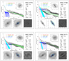 |
Fig. E.1. continued. |
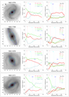 |
Fig. E.2. continued. |
All Tables
Mean parameter values of barlenses in group (a), and of barlenses and separate bulge components in group (b).
Mean parameter values calculated for the different structure components using the CALIFA V500 data cubes (e.g., Sánchez et al. 2016a).
Barlens (bl) identifications in the CALIFA survey, shown separately for the CALIFA “mother” and “extended” samples, and for the galaxies in which barlenses and X-shaped features appear at the same time.
Galaxies with X-shaped bars in the CALIFA survey, identified from the unsharp mask images.
Measured semimajor (a) and semiminor (b) axis lengths of bars, and barlenses, given in arcseconds.
All Figures
|
Fig. 1. Synthetic simulation images from Laurikainen & Salo (2017). In the left panels the direct image in the magnitude scale is shown, the middle panels show the contours of the same image, and the right panels show the unsharp mask image. In the four upper lines the galaxy inclination is fixed to i = 60°, whereas the azimuthal angle ϕ with respect to the bar major axis varies. In the lowest line the same model is seen edge-on. The initial values of the simulation contain a small classical bulge with bulge-to-total ratio B/T = 0.075. During the simulation a bar with a vertically thick inner barlens component forms. |
| In the text | |
|
Fig. 2. Examples of the X-shaped bars. Left panels show the bar regions of the combined r′ + g′ + i′ SDSS mosaic images. Right panels show the unsharp mask images made for the r′-band mosaics, using the same image cuts. |
| In the text | |
|
Fig. 3. Galaxy inclination plotted as a function of the absolute B-band galaxy magnitude. The parameter values are from HyperLEDA. Gray dots indicate galaxies in the complete CALIFA sample of 1064 galaxies, green symbols show the X-shaped bars, red symbols the barlenses, and blue symbols the galaxies in which both features appeared. Filled red circles denote the barlens galaxies for which we made the decomposition, and open squares the 26 galaxies, for which the V500 grating SSP data cubes were also available. |
| In the text | |
|
Fig. 6. Relation between the visually estimated barlens size (semimajor axis of the fitted ellipse) and the barlens effective radius that comes out in our decompositions. The dashed line shows the relation Re = 0.36a, which was obtained by a linear fit, to the values obtained in the decompositions in which barlens Re was a free parameter. The linear correlation coefficient between Re and a is 0.83. |
| In the text | |
|
Fig. 4. Three decomposition models (B/D, B/D/bar, and B/D/bar/bl) shown for the galaxies NGC 7563 and NGC 5406. In the upper panels, the 2D representations of the surface brightness profiles are shown; black dots show the fluxes of the image pixels as a function of distance in the sky plane, and the white dots those of the total model images. The colors illustrate the fitted models of various structure components. Lower panels: r′-band mosaic images overplotted with the effective radii of the fitted models. |
| In the text | |
|
Fig. 5. Bulge-to-total (B/T) flux ratios for the 46 galaxies decomposed in this study. The values in three type of models are shown: bulge/disk (B/D, upper panel), bulge/disk/bar (B/D/bar, middle panel) and bulge/disk/bar/bl (B/D/bar/bl, lower panel). The B/T values for the individual galaxies are shown in Table 1. Compared to the B/D and B/D/bar models, the number of the B/D/bar/bl models is smaller because only half of the decomposed galaxies were fitted with a separate bulge component |
| In the text | |
|
Fig. 7. Surface brightness profiles for the theoretical Ferrers function using different values for the parameters α and β, related to the sharpness of the outer truncation and the central slope of the profile, respectively. The lines indicate different combinations of α and β; the red line shows the typical values obtained in the current study. The different curves are normalized to correspond to the same total bar flux. |
| In the text | |
|
Fig. 8. Three decompositions (B/D, B/D/bar, and B/D/bar/bl) for a simulation snapshot taken from Salo & Laurikainen (2017). The model is explained in the text. The meaning of the lines and symbols are the same as in Fig. 4. |
| In the text | |
|
Fig. 10. Examples of our multicomponent decompositions. Large panel: black dots show the surface brightnesses (r′ magnitude/arcsec2) of the pixels in the two-dimensional image, white dots the values in the final model image, and the colors the values corresponding to the different structure components of the model. Bulges, disks, and barlenses were fitted with a Sérsic function, and bars with a Ferrers function. The decomposition parameters, galaxy masses (log M⋆), galaxy inclinations (i), and Hubble stages (T) are shown in the upper right. Lower panels (from left to right): region of the r′-band SDSS mosaic image, the same image with the model components plotted on top of that, and the unsharp mask image. The image in the large panel shows the full galaxy image. For more examples, see Appendix E. |
| In the text | |
|
Fig. 9. Twenty-six barlens galaxies are divided into groups (a; upper panel) and (b; lower panel) as explained in Sect. 6. The blue histograms indicate the barlens flux fraction BL/T. Additionally, the red histogram (same as in Fig. 5, lowermost frame) in the lower frame shows the relative fluxes of the separate bulge components in the group (b) galaxies. |
| In the text | |
|
Fig. 11. Illustration of the measured galaxy regions, as defined in Sect. 7.2. Left panel: original r′-band mosaic image of NGC 5000 to show the bar region. Right panel: definitions of the regions. Red indicates galaxy center (C), turquoise indicates barlens (bl), blue indicate bar, and green indicates disk. |
| In the text | |
|
Fig. 12. Differences of the parameter values between the central galaxy regions and barlenses (C-BL), and between barlenses and bars (BL-BAR), are shown for the sample of 26 galaxies. Positive and negative deviations are shown with red and blue colors, respectively. The parameters are the same as in Table 3. |
| In the text | |
|
Fig. 13. Amount of contamination in the measurements of average values for different structure components from decomposition models from Sect. 5. The plot shows the distribution of the fractional contribution of the component itself to the total flux in the measurement region of that structure component, as defined in Sect. 7.2. |
| In the text | |
|
Fig. 15. Cumulative distributions of the average ages and metallicities in the different structure components, measured in regions as defined in Fig. 11. Included are the 26 barlens galaxies in our sample. The V500 data cubes by Sánchez et al. (2016a) (SSP.cube.fits) were used, loaded from the CALIFA database. Distributions are based on median values of the pixels covered by the structure components; practically identical distributions are obtained when using flux-weighted means. Labels indicate the p-values in KS-tests comparing the distribution with that of barlenses; p < 0.05 indicates a statistically significant difference. |
| In the text | |
|
Fig. 14. Left: deprojected SDSS r′-band mosaic image. Overplotted are the elliptical zones (see Sect. 7.2) used in the measurement of structure averages shown deprojected to the disk plane (original measurements were carried out in non-deprojected images). Middle: Fractions of stars in the three stellar age bins, as a function of the deprojected radial distance. The profiles are constructed using the V500 grating data cubes from Sánchez et al. (2016b), loaded from CALIFA database (SFH.cube.fits). These profiles correspond to averages over mass and luminosity-weighted star formation histories. The vertical lines show the deprojected semimajor axis lengths of the bars, barlenses, and the central galaxy regions. Right: fractions of stars in four different metallicity bins, as given in the CALIFA data cubes. The meaning of the vertical lines are the same as in the middle panel. For more examples, see Appendix E. |
| In the text | |
|
Fig. 16. Distributions of the minor-to-major (b/a) axis ratios of the galaxies hosting barlenses (bl; our sample 2) and X-shaped features (X; our sample 3) in the CALIFA sample. The combined bl+X distribution is compared with that of the complete sample of CALIFA galaxies (our sample 1), scaled by a factor of 0.25. The histograms for both bl and X include the 15 galaxies in which both features appear. In the combined bl+X histogram these galaxies are included only once. The b/a values are from our measurements when available, otherwise from HyperLEDA. However, use of HyperLEDA inclinations would yield very similar distributions. |
| In the text | |
|
Fig. 17. Sixteen barlens galaxies common with Méndez-Abreu et al. (2018) and this work are shown in the V/σ−ϵ plane. The parameters refer to values measured within one Re of the bulge (see Table 2 in Méndez-Abreu et al. 2018). They are corrected for pixelation and resolution effect (as explained in the original paper). The solid line shows the expected relation for rotationally flattened oblate spheroids seen edge-on, following the approximation |
| In the text | |
|
Fig. 18. Relative flux of barlens (bl/T) as a function of velocity dispersion σ of the same component. The barlenses in our subsample of 26 galaxies are plotted. |
| In the text | |
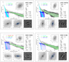 |
Fig. E.1. Examples of our multicomponent decompositions. See caption of Fig. 10 for explanation. |
| In the text | |
|
Fig. E.1. continued. |
| In the text | |
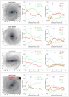 |
Fig. E.2. Deprojected SDSS r′-band mosaic image. See caption of Fig. 14 for explanation. |
| In the text | |
|
Fig. E.2. continued. |
| In the text | |
Current usage metrics show cumulative count of Article Views (full-text article views including HTML views, PDF and ePub downloads, according to the available data) and Abstracts Views on Vision4Press platform.
Data correspond to usage on the plateform after 2015. The current usage metrics is available 48-96 hours after online publication and is updated daily on week days.
Initial download of the metrics may take a while.