© ESO 2018

1 Introduction

In recent years, a number of experiments have dramatically increased the amount of data pertaining to the polarized thermal emission from Galactic dust in the submillimetre (e.g. Matthews et al. 2009; Ward-Thompson et al. 2009; Dotson et al. 2010; Bierman et al. 2011; Vaillancourt & Matthews 2012; Hull et al. 2014; Koch et al. 2014; Fissel et al. 2016). Chief among these is Planck¹, which provided the first full-sky map of this emission, leading to several breakthrough results. It was thus found that the polarization fraction p in diffuse regions of the sky can reach values above 20% (Planck Collaboration Int. XIX 2015), confirming results previously obtained over one fifth of the sky by the Archeops balloon-borne experiment (Benoît et al. 2004; Ponthieu et al. 2005). Furthermore, the polarization fraction is anti-correlated with the local dispersion $\mathcal{S}$ of polarization angles ψ (Planck Collaboration Int. XIX 2015; Planck Collaboration Int. XX 2015), and the decrease of the maximum observed p with increasing gas column density N_H may be fully accounted for, at the scales probed by Planck (5′ at 353 GHz), by the tangling of the magnetic field on the line of sight (LOS; Planck Collaboration Int. XX 2015). Similar anti-correlations were found with the BLASTPol experiment (Fissel et al. 2016) at higher angular resolution (a few tens of arcseconds) towards a single Galactic molecular cloud (Vela C). At 10′ scales, and over a larger sample of clouds, Planck data showed that the relative orientation of the interstellar magnetic field B and filamentary structures of dust emission is consistent with simulated observations derived from numerical simulations of sub- or trans-Alfvénic magnetohydrodynamical (MHD) turbulence (Planck Collaboration Int. XXXV 2016), and starlight polarization data in extinction yield similar diagnostics (Soler et al. 2016). In diffuse regions, the preferential alignment of filamentary structures with the magnetic field (Planck Collaboration Int. XXXII 2016; Planck Collaboration Int. XXXVIII 2016) is linked to the measured asymmetry between the power spectral amplitudes of the so-called E- and B-modes of polarized emission. Finally, measurements of the spatial power spectrum of polarized dust emission showed that it must be taken into account in order to obtain reliable estimates of the cosmological polarization signal (Planck Collaboration Int. XXX 2016).

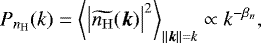
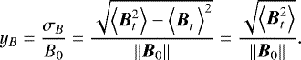
With this wealth of data, we may be able to put constraints on models of magnetized turbulence in the interstellar medium (ISM), provided we can extract the relevant information from polarization maps. Of particular interest are the statistical properties of the Galactic magnetic field (GMF) B. Let us write this as a sum B = B₀ + B_t of a uniform, large-scale component B₀, and a turbulent component B_t that has a null spatial average, ⟨B_t⟩ = 0. The statistical properties in question are then essentially modelled by two quantities, i) the ratio of the turbulent component to the mean, y_B = σ_B∕B₀, where ${\sigma }_B^2=\langle {\text{ B}}_t^2\rangle$ and B₀ = ||B₀||, and ii) the spectral index β_B, which characterizes the distribution of power of B_t across spatial scales, through the relationship P(k) ∝ k^−β_B, where k is the wavenumber and P(k) is the power spectrum ².

As mentioned above, Planck Collaboration Int. XXXV (2016) studied the relative orientation between the magnetic field, probed by polarized thermal dust emission, and filaments of matter in and around nearby molecular clouds. They find that this relative orientation changes, from mostly parallel to mostly perpendicular, as the total gas column density N_H increases, which is a trend observed in simulations of trans-Alfvénic or sub-Alfvénic MHD turbulence (Soler et al. 2013). Using the Davis-Chandraskehar-Fermi method (Chandrasekhar & Fermi 1953) improved by Falceta-Gonçalves et al. (2008) and Hildebrand et al. (2009), and from their results, we estimated the ratio y_B to be in the range 0.3–0.7. Planck Collaboration Int. XXXII (2016) studied that same relative orientation in the diffuse ISM at intermediate and high Galactic latitudes, and their estimate of y_B is in the range 0.6–1.0 with a preferred value at 0.8. These estimates are confirmed in Planck Collaboration Int. XLIV (2016), which presents a fit of the distributions of polarization angles and fractions observed by Planck towards the southern Galactic cap. They use a model of the GMF involving a uniform large-scale field B₀ and a small number (N_l ≃ 7) of independent “polarization layers” on the LOS, each of which accounts for a fraction 1∕N_l of the total unpolarized emission. Within each layer, the turbulent component B_t of the magnetic field, which is used to compute synthetic Stokes Q and U maps, is an independent realization of a Gaussian two-dimensional random field with a prescribed spectral index β_B. Through these fits, they confirm the near equipartition of large-scale and turbulent components of B, with y_B ≃0.9. They also provide a rough estimate of the magnetic field’s spectral index β_B in the range two to three. This work was complemented in Vansyngel et al. (2017), using the same framework, but including observational constraints on the power spectra of polarized thermal dust emission. These authors are able to constrain β_B ≃ 2.5, an exponent which is compatible with the rough estimate of Planck Collaboration Int. XLIV (2016), and close to that measured for the total intensity of the dust emission. We note that their exploration of the parameter space does not allow for an estimation of the uncertainty on β_B.

In Planck Collaboration Int. XXXII (2016), Planck Collaboration Int. XLIV (2016) and Vansyngel et al. (2017), the description of structures, in both dust density and magnetic field, along the LOS is reduced to the bare minimum, while statistical properties in the plane of the sky (POS) are modelled through y_B and β_B. Orthogonal approaches have also been pursued (e.g. Miville-Deschênes et al. 2008; O’Dea et al. 2012), in which the turbulent component of the magnetic field is modelled along each LOS independently from the neighbouring ones, as a realization of a one-dimensional Gaussian random field with a power-law power spectrum. In this type of approach there is no correlation from pixel to pixel on the sky, and such studies seek to exploit the depolarization along the LOS, ratherthan spatial correlations in the POS, to constrain statistical properties of the interstellar magnetic field.

We sought to explore another avenue, taking into account statistical correlation properties of B in all three dimensions, as well as properties of the dust density field, building on methods developed in Planck Collaboration Int. XX (2015) to compare Planck data with synthetic polarization maps. In that paper, the synthetic maps are computed from data cubes of dust density n_d and magnetic field B produced bynumerical simulations of MHD turbulence. One could imagine generalizing this approach, taking advantage of the ever-increasing set of such simulations (see, e.g., Hennebelle et al. 2008; Hennebelle 2013; Hennebelle & Iffrig 2014; Inutsuka et al. 2015; Seifried & Walch 2015). However, this would be impractical for two main reasons: i) these simulations often have a limited inertial range over which the power spectrum has a power-law behaviour, and ii) a systematic study exploring a wide range of physical parameters with sufficient sampling is not possible due to the computational cost of each simulation.

We therefore propose an alternative approach, which is to build simple, approximate, three-dimensional models for the dust density n_d and the magnetic field B, allowing us to perfectly control the statistical properties of these three-dimensional fields, and to fully explore the space of parameters characterizing them. With this approach, we are able to perform a statistically significant number of simulated polarization maps for each set of parameters. Actual observations may then be compared to these simulated maps, using least-square analysis methods, to extract best-fitting parameters, in particular the spectral index of the magnetic field, β_B, and the ratio of turbulent to regular field, y_B.

The paper is organized as follows: Sect. 2 presents the method used to build simulated thermal dust polarized emission maps using prescribed statistical properties for n_d and B. Observables derived from these maps, serving as statistical diagnostics of the input parameters, are presented in Sect. 3. In Sect. 4, we describe the Markov chain Monte Carlo (MCMC) analysis method devised to explore the space of input parameters for a given set of polarization maps. The validation of the method and its application to actual observations of polarized dust emission from the Polaris Flare molecular cloud observed by Planck are given in Sect. 5. Finally, Sect. 6 discusses our results and offers conclusions. Several appendices complement our work. Appendix A presents further statistical properties of the model dust density fields. Appendix B details the likelihood used in the MCMC analysis. Finally, Appendix C details the χ² parameter used to estimate the goodness of fit.

2 Building synthetic polarized emission maps

In this section, we first describe the synthetic dust density and magnetic field cubes we have used in our analysis. We then explain how simulated polarized emission maps are built from these cubes.

2.1 Fractional Brownian motions

The basic ingredients to synthesize polarized thermal dust emission maps are three-dimensional cubes of dust density n_d and magnetic field B, which we build using fractional Brownian motions (fBm) (Falconer 1990). An N-dimensional fBm X is a random field defined on ${ℝ}^N$ such that $\langle {\left[X\left(r_2\right)-X\left(r_1\right)\right]}^2\rangle \propto \left|\right|r_2-r_1|{|}^{2H}$, for any pair of points (r₁, r₂). H is called the Hurst exponent. These fBm fields are usually built in Fourier space³, $$\text{widetilde}X(k)=A(k)\exp \left[i{\varphi }_X(k)\right],$$(1)

by specifying amplitudes that scale as a power-law of the wavenumber k = ||k||, $$A(k)=A_0{k}^{-{\beta }_X/2},$$(2)

with β_X = 2H + N the spectral index, and phases drawn from a uniform random distribution in [−π, π], subject to the constraint ϕ_X(−k) = −ϕ_X(k) so that X is real-valued. Their power spectra are therefore power laws, $$P_X(k)=\text{left}<{\left|\text{widetilde}X(k)\right|}^2\text{right}{>}_{\left|\right|k\left|\right|=k}\propto k^{-{\beta }_X},$$(3)

where the average is taken over the locus of constant wavenumber k in Fourier space. Such fields have been used previously as toy models for the fractal structure of molecular clouds, in both density and velocity space (Stutzki et al. 1998; Brunt & Heyer 2002; Miville-Deschênes et al. 2003; Correia et al. 2016).

2.2 Dust density

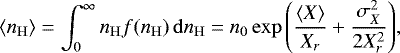
In our approach, the dust density n_d is taken to be proportional to the total gas density n_H, so that the dust optical depth within each cell is also proportional to n_H (see the derivation of polarization maps in Sect. 2.4). Therefore, we intended to model n_H from numerical realizations of three-dimensional fBm fields built in Fourier space. These have means that are defined by the value chosen for the null-wavevector amplitude A(0), so if one wished to use such a synthetic random field X directly as a model for the positive-valued n_H, one would be required to choose n_H = X′ = X − a with a ≥min(X) a constant. However, since the distributions of these fields in three dimensions are close to Gaussian, their ratio of standard deviation to mean is typically ${\sigma }_{X^{\prime }}/\langle X^{\prime }\rangle \lesssim 0.3$, which is much too small compared to observational values. For instance, the total gas column density fluctuation ratios ${\sigma }_{N_{\text{H}}}/\text{left}<N_{\text{H}}\text{right}>$ in the ten nearby molecular clouds selected for study in Planck Collaboration Int. XX (2015) are in the range 0.3–1, and one should keep in mind that these are only lower bounds for fluctuation ratios in the three-dimensional density field n_H.

We remedied this shortcoming by taking X to represent the log-density, i.e., n_H is given by $$n_{\text{H}}=n_0\exp \left(\frac{X}{X_r}\right),$$(4)

where X is a three-dimensional fBm field with spectral index β_X, and X_r and n₀ are positive parameters. The n_H fields built in this fashion have simple and well-controlled statistical properties. First, their probability distribution functions (PDF) are log-normal, which allows, through an adequate choice of X_r, to set the fluctuation level of the density field $y_n={\sigma }_{n_{\text{H}}}/\langle n_{\text{H}}\rangle$ to any desired value. Second, their power spectra, as azimuthal averages in Fourier space, retain the power-law behaviour of the original fBm X, $$P_{n_{\text{H}}}(k)=\text{left}<{\left|\text{widetilde}{n}_{\text{H}}(k)\right|}^2\text{right}{>}_{\left|\right|k\left|\right|=k}\propto k^{-{\beta }_n},$$(5)

although the spectral indices β_n may deviate significantly from β_X. An example of such a field is shown in Fig. 1, which represents the total gas column density N_H derived from a gas volume density n_H built as the exponential of a 120 × 120 × 120 fractional Brownian motion with zero mean, unit variance, and spectral index β_X = 2.6. The parameters of the exponentiation are X_r = 1.2 and n₀ = 20 cm⁻³, and the gridis chosen so that the extent of the cube is 30 pc on each side, corresponding to a pixel size of 0.25 pc. More detail on the properties of these fields are given in Appendix A.

The density fields built in this fashion are of course only a rough statistical approximation for actual interstellar density fields. For instance, they are unable to reproduce the filamentary structures observed in dust emission maps (André et al. 2010; Miville-Deschênes et al. 2010). These structures cannot be captured by one- and two-point statistics such as those used here, and require a description involving higher-order moments or the Fourier phases (see, e.g., Levrier et al. 2006; Burkhart & Lazarian 2016).

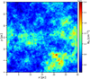Fig. 1 Total gas column density NH, derived froma synthetic density field nH built by exponentiation of a fBm field with spectral index βX = 2.6 and size 120 × 120 × 120 pixels. The volume density fluctuation level is yn = 1, and the column density fluctuation level is $y_{N_{\text{H}}}\simeq 0.25$.

2.3 Magnetic field

To obtain a synthetic turbulent component of the magnetic field B_t with null divergence and controlled power spectrum, we started from a vector potential A built as a three-dimensional fractional Brownian motion. To be more precise, each Cartesian component A_λ of A is a fBm field, $$\text{nnwidetilde}{A}_{\lambda }(k)={\mathcal{A}}_0{k}^{-{\beta }_A/2}\exp \left[i{\varphi }_{A_{\lambda }}(k)\right],$$(6)

where the spectral index β_A and the overall normalization parameter ${\mathcal{A}}_0$ are independent of the Cartesian component λ = x, y, z considered. Using the definition of the magnetic field from the vector potential B_t,λ = ϵ_λμν∂_μA_ν, with the Einstein notation, where ϵ_λμν is the Levi-Civita tensor, and the derivation relation in Fourier space $$\text{nnwidetilde}{\partial }_{\lambda }F=i{k}_{\lambda }\text{ widetilde}F$$(7)

we have the expression of the components of B_t in Fourier space $$\text{widetilde}{B}_{t,\lambda }(k)={\mathcal{A}}_0{ϵ}_{\lambda \mu \nu }i{k}_{\mu }{k}^{-{\beta }_A/2}\exp \left[i{\varphi }_{A_{\nu }}(k)\right]$$(8)

As it should, this expression corresponds to a divergence-free turbulent magnetic field, $$i{k}_{\lambda }\text{widetilde}{B}_{t,\lambda }=0.$$(9)

Writing k_μ = kf_μ, with $f=\left(\sin \vartheta \cos \phi ,\sin \vartheta \sin \phi ,\cos \vartheta \right)$, the power spectrum of each component of B_t is then $$P_{B_{t,\lambda }}(k)={\mathcal{A}}_0^2{k}^{2-{\beta }_A}\text{left}<{\left|{ϵ}_{\lambda \mu \nu }{f}_{\mu }\exp \left[i{\varphi }_{A_{\nu }}(k)\right]\right|}^2\text{right}{>}_{\left|\right|k\left|\right|=k}.$$(10)

The last factor is essentially independent of the wavenumber k, so the spectral index of each component of B_t is 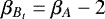${\beta }_{B_t}={\beta }_A-2$. After Fourier-transforming back to real space, B_t is shifted and scaled so that it has zero mean and a standard deviation σ_B of 5 μG, a value typical of the interstellar magnetic field (see, e.g., Haverkorn et al. 2008, and references therein).

The model magnetic field B is obtained by adding a uniform⁴ vector field B₀ to that turbulent magnetic field B_t. The effect in Fourier space is limited to a modification for k = 0 only, so the spectral index of each component B_λ of the total magnetic field is the same as that of B_t,λ, i.e., $$P_{B_{\lambda }}(k)\propto k^{2-{\beta }_A}.$$(11)

This means that the resulting magnetic fields thus only display anisotropy in the k =0 mode, and not at the other scales. This is a limitation of our model, which is thus not fully consistent with observations of the magnetic field structure (Planck Collaboration Int. XXXV 2016), but it is sufficient for our purposes.

The uniform field B₀ which is added to the turbulent field B_t is defined byits norm B₀ and a pair of angles, γ₀ and χ₀, which are respectively the angle between the magnetic field and the POS, and the position angle of the projection of B₀ in the POS, counted positively clockwise from the north-south direction (see Fig. 14 of Planck Collaboration Int. XX 2015). The total magnetic field’s direction in three-dimensional space is characterized by angles γ and χ defined in the same way. The ratio of the turbulent to mean magnetic field strengths is then defined by $$y_B=\frac{{\sigma }_B}{B_0}=\text{frac{sqrt{left}<{\text{B}}_t^2\text{right}>-\text{left}<{\text{B}}_t^{\text{phantom}2}\text{right}{>}^2\text{}}}\left|\right|{\text{B}}_0\left|\right|=\text{frac{sqrt{left}<{\text{B}}_t^2\text{right}>\text{}}}\left|\right|{\text{B}}_0\left|\right|.$$(12)

Figure 2 shows an example of a synthetic magnetic field B generated in this fashion, and defined on the same 120 × 120 × 120 pixels grid that was used for the gas density model described in Sect. 2.2. The parameters used for this specific realization are β_A = 5, y_B = 1, and χ₀ = γ₀ = 0°. The distribution functions (DF) of the components of such model magnetic fields are Gaussian, as shown in Fig. 3, and their power spectra are power laws of the wavenumber, as shown in Fig. 4, with a common spectral index β_B that is related to the input β_A by β_B = β_A − 2.

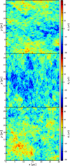Fig. 2 Synthetic magnetic field B built using Eq. (8). The spectral index of the vector potential is βA = 5 and the size of the cubes is 120 × 120 × 120 pixels, corresponding to 30 pc on each side. Shown are two-dimensional slices through the cubes of the components Bx (top), By (middle), and Bz (bottom). The ratio of the fluctuations of the turbulent component Bt to the norm of the uniform component B0 is yB =1 in this particular case, with angles χ0 = γ0 = 0°.

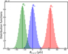Fig. 3 Distribution functions of the components Bx, By, and Bz of a model magnetic field B = B0 + Bt built on a grid 120 × 120 × 120 pixels using Eq. (8) with βA = 5, and a mean, large-scale magnetic field B0 defined by the angles χ0 = 0° and γ0 = 60°, and a norm B0 = 50 μG such that the fluctuation level is yB = 0.1. The vertical lines represent the projected values of the large scale magnetic field B0x = B0 sinχ0 cosγ0, B0y = −B0 cosχ0 cosγ0 and B0z = B0 sinγ0. See Fig. 14 in Planck Collaboration Int. XX (2015) for the definition of angles.

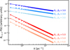Fig. 4 Powerspectra of the components Bx, By and Bz of a model magnetic field B = B0 + Bt built on a grid 120 × 120 × 120 pixels using Eq. (8) with βA = 3 (different shades of blue for the three components) and βA = 5 (different shades of red for the three components). The power spectra are normalized differently so as to allow comparison between them. The fitted power-laws shown as solid lines yield spectral indices βB = 1 and βB = 3, in agreement with Eq. (11). These are the power spectra of the same particular realizations shown in Fig. 2.

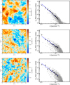Fig. 5 Left column row: example maps (from top to bottom: total intensity Im on a logarithmic scale, Stokes Qm, and Stokes Um) from simulation A (see Sect. 5 and Table 3). Right column: corresponding power spectra. The grey points represent the two-dimensional power spectra, while the black dots represent the azimuthal averages in Fourier space in a set of wavenumber bins, and the blue line is a power-law fit to the black points.

2.4 Polarization maps

Once cubes of total gas density n_H and magnetic field B are available, maps of Stokes parameters I, Q, and U at 353 GHz (the frequency of the Planck channel with the best signal-to-noise ratio in polarized thermal dust emission) are built by integrating along the LOS through the simulation cubes, following the method in Planck Collaboration Int. XX (2015): $$\begin{array}{lll}{I}_0\hfill & =\hfill & {\displaystyle \int S_{\nu }}\left[1-p_0\left({\cos }^2\gamma -\frac{2}{3}\right)\right]{\sigma }_{353}{n}_{\text{H}}\text{\hspace{0.17em}d}z;\hfill \\ Q_0\hfill & =\hfill & {\displaystyle \int p_0}{S}_{\nu }\cos \left(2\varphi \right){\cos }^2\gamma {\sigma }_{353}{n}_{\text{H}}\text{\hspace{0.17em}d}z;\hfill \\ U_0\hfill & =\hfill & {\displaystyle \int p_0}{S}_{\nu }\sin \left(2\varphi \right){\cos }^2\gamma {\sigma }_{353}{n}_{\text{H}}\text{\hspace{0.17em}d}z.\hfill \end{array}$$

In these equations, we take the intrinsic polarization fraction parameter p₀ to be uniform, and the source function S_ν = B_ν(T_d) to be that of a black body with an assumed uniform dust temperature T_d. The dust opacity at this frequency σ₃₅₃ is taken to vary with N_H, following Fig. 20 in Planck Collaboration XI (2014) for X_CO = 2 10²⁰ H₂ cm^-2 K^-1 km^-1 s, and propagating the associated errors. The order of magnitude of the dust opacity is around σ₃₅₃ ≈ 10⁻²⁶ cm². The values of N_H considered in our study are typically at most a few 10²¹ cm⁻², so the optically thin limit applies in the integrals of Eqs. (13)–(15). The angle ϕ is the local polarization angle, which is related to the position angle⁵ χ of the magnetic field’s projection on the POS at each position on the LOS by a rotation of 90° (see definitions of angles in Planck Collaboration Int. XX 2015).

The n_H and B cubes are built on a grid which is 132 × 132 pixels in the POS and N_z pixels in the z direction (that of the LOS). The cells have a physical size δ = 0.24 pc in each direction, so the depth d = N_z δ of the cloud is a free parameter in our analysis, and the Stokes maps built from Eqs. (13)–(15) are 32 pc in both x and y directions.

2.5 Noise and beam convolution

In order to proceed with the analysis of observational data, one cannot use these model Stokes maps directly: it is necessary to properly take into account noise and beam convolution. Anticipating somewhat the description of the Planck data we shall use as an application of the method, the 353 GHz noise covariance matrix maps are taken directly from the Planck Legacy Archive⁶ and are part of the 2015 public release of Planck data (Planck Collaboration I 2016), $$\Sigma =\left(\begin{array}{ccc}{\sigma }_{II}& {\sigma }_{IQ}& {\sigma }_{IU}\\ {\sigma }_{QI}& {\sigma }_{QQ}& {\sigma }_{QU}\\ {\sigma }_{UI}& {\sigma }_{UQ}& {\sigma }_{UU}\end{array}\right).$$(16)

Noise is added to the model Stokes maps pixel by pixel, as $$I_n=I_0+n_I{Q}_n=Q_0+n_Q{U}_n=U_0+n_U,$$(17)

where n_I, n_Q, and n_U are random values drawn from a three-dimensional Gaussian distribution with zero mean and characterized by the noise covariance matrix Σ. To preserve the properties of Planck noise, the random values are directly drawn from the Healpix (Górski et al. 2005) covariance matrix maps and added to the simulated maps after a gnomonic projection of the region under study, in our case the Polaris Flare molecular cloud.

The resulting Stokes I_n, Q_n, and U_n maps are then placed at a distance⁷ D = 140 pc, so that the angular size of each pixel is about 6′, and then convolved by a circular 15′ full-width at half maximum (FWHM) Gaussian beam $\mathcal{B}$. To avoid edge effects, only the central 120 × 120 pixels of the convolved maps $I_{\text{m}}=\mathcal{B}\otimes I_n$, $Q_{\text{m}}=\mathcal{B}\otimes Q_n$, and $U_{\text{m}}=\mathcal{B}\otimes U_n$ are retained, corresponding to a field of view (FoV) of approximately 12°. With this approach, the model maps (I_m, Q_m, U_m) are fit to be compared to actual Planck data, which we discuss in Sect. 5.2.

3 Observables

From the model maps above, we build an ensemble of derived maps, starting with the normalized Stokes maps $$i=\frac{I_{\text{m}}}{\langle I_{\text{m}}\rangle }q=\frac{Q_{\text{m}}}{I_{\text{m}}}u=\frac{U_{\text{m}}}{I_{\text{m}}}$$(18)

where ⟨I_m⟩ is the spatial average of the model Stokes I_m map. Then we define the polarization fraction, which requires us to note that since our models include noise, we should not use the “naïve” estimator (Montier et al. 2015a,b) $$p=\frac{\sqrt{Q_{\text{m}}^2+U_{\text{m}}^2}}{I_{\text{m}}},$$(19)

but rather the modified asymptotic (MAS) estimator proposed by Plaszczynski et al. (2014) $$p_{\text{MAS}}=p-b^2\frac{1-e^{-p^2/b^2}}{2p}$$(20)

where the noise bias parameter b² derives from the elements of the noise covariance matrix Σ (see Montier et al. 2015b). Next, we define the polarization angle $$\psi =\frac{1}{2}\text{atan}\left(U_{\text{m}},Q_{\text{m}}\right)$$(21)

where the two-argument atan function lifts the π-degeneracy of the usual atan function. We note that this expression means that the polarization angle is defined in the Healpix convention.

We also build maps of the polarization angle dispersion function $\mathcal{S}$ (Planck Collaboration Int. XIX 2015; Planck Collaboration Int. XX 2015; Alina et al. 2016), which quantifies the local dispersion of polarization angles at a given lag δ and is defined by $$\mathcal{S}(r,\delta )=\sqrt{\frac{1}{\mathcal{N}}{\sum }_{i=1}^{\mathcal{N}}{\left[\psi \left(r+{\delta }_i\right)-\psi \left(r\right)\right]}^2}$$(22)

where the sum is performed over the $\mathcal{N}$ pixels r + δ_i whose distance to the central pixel r lies between δ∕2 and 3δ∕2. For the sake of consistency with the analysis performed on simulated polarization maps in Planck Collaboration Int. XX (2015), we take δ = 16′.

Finally we build the column density and optical depth τ₃₅₃ maps from the dust density cube using $$N_{\text{H}}={\displaystyle \int n_{\text{H}}}\text{\hspace{0.17em}d}z\text{\hspace{1em} and \hspace{1em}}{\tau }_{353}={\sigma }_{353}\left(N_{\text{H}}\right)\times N_{\text{H}}$$(23)

with the ${\sigma }_{353}\left(N_{\text{H}}\right)$ conversion⁸ from Planck Collaboration XI (2014). A temperature map T_obs is also created using the anti-correlation with the column density N_H observed in the data. This “dust temperature map” does not pretend to model reality but since T_d is one of the parameters of the model, the fitting algorithm requires a map whose mean value should yield T_d.

4 Exploring the parameter space

The goal of this paper is to constrain the physical parameters of molecular clouds. In particular we aim to constrain the spectral indices of the dust density and of the turbulent magnetic field, using Planck polarization maps and a grid of model maps built as explained inthe previous section.

4.1 Parameter space

The nine physical parameters that are explored in this paper using fBm simulations are summarized in Table 1. They are sufficient to describe the one-point and two-point statistical properties of the dust density and magnetic field models. We note that contrary to the method in Planck Collaboration Int. XLIV (2016), the FoV of the maps analysed in the following (approximately 12°) is too small to contain remarkable features that could be used to constrain the angle γ₀ that the mean magnetic field makes with the POS. In such small FoVs, there is a degeneracy between y_B and γ₀ which cannot be lifted. Consequently, we chose not to try to fit for γ₀ and y_B, but for the ratio of the turbulent magnetic field RMS to the mean magnetic field in the POS, i.e., $$y_B^{\text{POS}}=\frac{{\sigma }_B}{B_0^{\text{POS}}}=\text{frac{sqrt{left}<{\text{B}}_t^2\text{right}>\text{}}}\left|\right|{\text{B}}_0\left|\right|\cos {\gamma }_0=\frac{y_B}{\cos {\gamma }_0}.$$(24)

This analysis was applied to the Polaris Flare (see Sect 5.2), so the priors were chosen to be flat over a reasonably large range, to cover the expected physical values of the molecular cloud under consideration, but they are necessary for the analysis to converge. The cloud’s average column density is of the order ⟨N_H⟩≈ 10²¹ cm⁻² (Planck Collaboration Int. XX 2015). This value was used to set the range for the prior on the depth d of the cube, with the limits of this range chosen in such a way that the average gas density ⟨n_H ⟩ lies between 10 and 500 cm⁻³, a reasonable assumption for the Polaris Flare molecular cloud. This translates to a total cube depth d of between 0.5 and 32.5 pc. The range used for the prior on β_n is justified by a number of observational studies (see, e.g., the review by Hennebelle & Falgarone 2012), and that on β_B is chosen based on the results from Vansyngel et al. (2017), but also on numerical studies of MHD turbulence (see, e.g., Perez et al. 2012; Beresnyak 2014). The fluctuation ratios y_n and $y_B^{\text{POS}}$ are explored in a logarithmic scale, as we are mainly interested in order of magnitude estimates for these parameters. The polarization maps being statistically identical when the angle χ₀ of the POS projection of the mean magnetic field is shifted by 180°, the prior on this parameter is such that this periodicity is applied when the Metropolis algorithm (see Sect. 4.3) draws values outside the given range. The priors chosen for T_d and p₀ are very large and do not play a role in the fitting procedure.

4.2 Comparing models with data

To set constraints on the parameters listed in Table 1, we built a likelihood function, which expresses the probability that a given set of synthetic polarization maps reproduce adequately actual observational data. From the model Stokes maps I_m, Q_m, and U_m, we derived a set of observables that are used in the likelihood function. These observables are given in Table 2. More precisely, we used i) the mean values for the optical depth τ₃₅₃ and the dust temperature T_obs, ii) the distribution functions (one-point statistics) of the I_m, Q_m, U_m, p_MAS, ψ, $\mathcal{S}$, and ${\tau }_{353}/\langle {\tau }_{353}\rangle$ maps, iii) the power spectra (two-point statistics) of the I_m,Q_m, and U_m maps, and iv) the pixel-by-pixel anti-correlation between $\mathcal{S}$ and p_MAS underlined by Planck Collaboration Int. XIX (2015). Indeed, we find that the shape of this two-dimensional distribution function also depends on the model parameters. Many other observables were tested but we have retained only those which bring constraints on the model parameters.

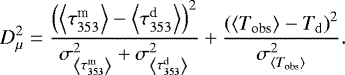
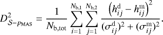
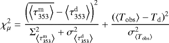
On the simulation side, N_r = 60 model realizations per set of parameter values are generated with their observables, to be compared with data. The N_r models differ by the random phases ϕ_X and ${\varphi }_{A_{\lambda }}$ used to build the dust density and magnetic field cubes (see Eqs. (1) and (8)), and by the random realization of the noise applied to the model (Eq. (17)). We checked that 60 simulations represent a statistically large enough sample to get robust averages and dispersions for the observables. The statistical properties of the observables derived from the observational polarization data are thus compared with the observables from those 60 models, through the evaluation of a parameter D² which quantifies the distance between data and one random realisation of the model, averaged over the N_r random realisations, with contributions associated to the various observables listed in Table 2, i.e., $$D^2=\frac{1}{N_r}{\sum }_{i=1}^{N_{\text{r}}}\left[D_{\mu }^2+{\sum }_o{D}_{\text{DF}(o)}^2+{\sum }_o{D}_{P(o)}^2+D_{\mathcal{S}-p_{\text{MAS}}}^2\right].$$(25)

This quantity is subtly different from the usual χ² (see Appendices B and C). The first term in Eq. (25) covers the observables $\langle {\tau }_{353}\rangle$ and $\langle T_{\text{obs}}\rangle$, and quantifies the difference between these values in the simulated maps and in the data. The second sum extends over the observable maps o in the set $\left\{I_{\text{m}},Q_{\text{m}},U_{\text{m}},p_{\text{MAS}},\psi ,\mathcal{S},{\tau }_{353}/\langle {\tau }_{353}\rangle \right\}$ and quantifies the difference between the distribution functions of these observables in synthetic maps and those of the same observables in the data. The third sum extends over the observable maps o in the set $\left\{I_{\text{m}},Q_{\text{m}},U_{\text{m}}\right\}$ and quantifies the difference between the power spectra of the simulated maps and those of the same maps in the data. Finally, the last term quantifies the discrepancy between the two-dimensional joint DFs of $\mathcal{S}$ and p_MAS in the data and in synthetic maps. We detail the computation of these various terms in Appendix B.

4.3 MCMC analysis

Given the vast parameter space to explore, we built a MCMC analysis (see, e.g. Brooks et al. 2011) that has the advantage to sample specifically the regions of interest in this space. We used a simple Metropolis-Hastings algorithm to build five Markov chains which sample the posterior probability distribution function (PDF) of the parameters listed in Table 1. The likelihood $\mathcal{L}$ of a set s of parameters is evaluated thanks to the D² criterion described in Sect. 4.2 and Appendix B as $$\mathcal{L}(s)\propto e^{-D^2(s)/2}\pi (s),$$(26)

with π(s) the prior associated to the parameters.

According to the Metropolis-Hastings algorithm, at each step q of the chain, parameters are drawn according to a multivariate probability distribution function whose covariance is set to allow for an efficient exploration of the parameter space, with an average given by the parameter values s_q−1 at step q − 1. If the likelihood for the new set of parameters, s_q, is larger than for the previous one, then the chain records the new set. Otherwise, the likelihood ratio $\mathcal{L}\left(s_q\right)/\mathcal{L}\left(s_{q-1}\right)<1$ is compared to a number α drawn randomly from a uniform distribution over [0, 1]. If the likelihood ratio is larger than α, the s_q set of parameters is kept, otherwise the chain duplicates the s_q−1 set, i.e., s_q = s_q−1. The posterior probability distribution function is then given by the occurence frequency of the parameters along the chains, after removal of the initial “burn-in” phase.

The priors used for each parameter are detailed in Table 1. For all parameters, flat priors are set covering a reasonable range of physical interest. If the Metropolis algorithm draws values outside of these priors we set π(s) = 0, except for the position angle of the mean magnetic field, χ₀, for which the 180° periodicity is used to bring back the angle inside its definition range when it is by chance drawn outside.

The convergence of the Markov chains is tested using the Gelman-Rubin statistics R (Gelman & Rubin 1992), which is essentially the ratio of the variance of the chain means to the mean of the chain variances. We estimated that the chains converged when R − 1 < 0.03 for the least-converged parameter. The convergence is also assessed by visually checking the D² and parameter evolutions along the chains.

The obtained nine-dimensional posterior probability distribution is generally not a multivariate Gaussian distribution. To quote an estimate of the best fit value for any one of the nine parameters and the associated uncertainties, we marginalize over the other eight parameters to obtain the one-dimensional posterior PDF for the remaining parameter. In the following, the

quoted best fit value for a parameter is the mean over this posterior PDF (which is less sensitive to binning effects than the maximum likelihood). As the PDFs are usually not Gaussian, we quote asymmetric error bars following the minimum credible interval technique (see, e.g., Hamann et al. 2007).

5 Results

5.1 Validation of the method

To validate the fitting method, we simulated four sets of model cubes and computed the corresponding I_m, Q_m, and U_m maps, including noise, with different values of the input parameters (hereafter simulations A, B, C, and D). The MCMC fitting procedure was run on these mock polarization data sets to check if it was able to recover the statistical properties of the input dust density and magnetic field cubes through the selected observables. The results are presented in Table 3. For the four sets of maps, the fitting method recovered the input values within the quoted uncertainties, after the convergence criteria for all the chains were reached⁹. This shows that this choice of observables is relevant to extract the input values from polarized thermal dust emission data within our model. To assess the goodness of fit of the model to the data, we use an a posteriori χ² test, as explained in Appendix C. In all four cases, we find that the match is very good, since $\text{left}<{\chi }_{\text{best}}^2\text{right}>\approx 1$. For illustration, the posterior probability contours for simulation A are presented in Fig. 6. We note that the MCMC procedure reveals correlations between the model parameters, which is not unexpected, for example, between $y_B^{\text{POS}}$ and p₀, or between y_n and ⟨n_H⟩. These trends are best visualized with the correlation matrix, shown in the upper right corner of Fig. 6.

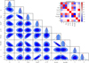Fig. 6 Constraints (posterior probability contours and marginalized PDFs) on the statistical properties of the dust density and magnetic field for the simulation A maps. On the posterior probability contours, the filled dark and light blue regions respectively enclose 68.3% and 95.4% of the probability, the black stars indicate the averages over the two-dimensional posterior PDFs, and the red circles indicate the input values for the simulation. In the plots showing the marginalized posterior PDFs, the light blue regions enclose 68.3% of the probability, the dashed blue lines indicate the averages over the posterior PDFs, and the solid red lines indicate the input values for the simulation. The upper right plot displays the correlation matrix between the fitted parameters.

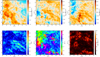Fig. 7 Planck 353 GHz maps of the Polaris Flare molecular cloud. The top row shows, from left to right, the total intensity I353 on a logarithmic scale, the Stokes Q353 map and the Stokes U353 map, while the bottom row shows the polarization fraction pMAS, the polarization angle ψ, and the polarization angle dispersion function $\mathcal{S}$. The τ353 and Tobs maps have the same aspects as the I353 map but with their own scales.

5.2 Application to the Polaris Flare

As an application of our method, we wish to constrain statistical properties of the turbulent magnetic field in the Polaris Flare, a diffuse, highly dynamical, non-starforming molecular cloud. There are several reasons for choosing this particular field. First, it has been widely observed: the structures of matter were studied in dust thermal continuum emission by, for example, Miville-Deschênes et al. (2010); the velocity field of the molecular gas was studied down to very small scales through CO rotational lines (Falgarone et al. 1998; Hily-Blant & Falgarone 2009); and the magnetic field was probed by optical stellar polarization data in Panopoulou et al. (2016). Second, as this field does not show signs of star formation, the dynamics of the gas and dust are presumably dominated by magnetized turbulence processes, without contamination by feedback from young stellar objects (YSOs). It therefore seems like an ideal test case for our method.

To thisaim, we used the full-mission Planck maps of Stokes parameters (I₃₅₃, Q₃₅₃, U₃₅₃) at 353 GHz and, as already mentioned, the associated covariance matrices from the Planck Legacy Archive. We also used the thermal dust model maps τ₃₅₃ and T_obs from the 2013 public release (Planck Collaboration XI 2014). All maps are at a native 4′.8 resolution in the Healpix format with N_side = 2048, and the Polaris Flare maps were obtained by projecting these onto a Cartesian grid with 6′ pixels, centred on Galactic coordinates (l, b) = (120°, 27°), with an FoVΔl = Δb = 12°. The maps ofI₃₅₃, Q₃₅₃, U₃₅₃, and τ₃₅₃ were then smoothed using a circular Gaussian beam, to obtain maps at a 15′ FWHM resolution. The covariance matrix maps were computed at the same resolution, using a set of Monte-Carlo simulations of pure noise maps, drawn from the original full-resolution covariance maps and smoothed at 15′. The maps of I₃₅₃, Q₃₅₃, U₃₅₃, p_MAS, ψ, and $\mathcal{S}$ obtained in this way are shown in Fig. 7.

We notethat the features of simulated Stokes maps are not located in the same regions as in the Polaris Flare maps. As the noise covariance matrices are the same for all the simulated maps, this means that the signal-to-noise ratio per pixel in the model I_m, Q_m and U_m maps is different for each set of parameters. However, the MCMC procedure is able to choose the parameter sets that give signal-to-noise ratios similar to those in the Planck maps.

The results of the analysis of the Planck polarized thermal dust emission data towards the Polaris Flare are presented in Table 4, and the posterior probability distribution contours are shown in Fig. 8. We find in particular that the spectral index of the turbulent component of the magnetic field is β_B = 2.8 ± 0.2, and that the spectral index of the dust density field is around β_n = 1.7 with a rather large uncertainty. The fluctuation ratio of the density field is about unity, y_n ≈ 1.6, and the magnitude of the large-scale magnetic field in the POS dominates slightly the RMS of the turbulent component, $y_B^{\text{POS}}\approx 0.65$, with a position angle χ₀ ≈−69°. The constraint on the depth of the cloud seems to indicate that d ≈ 13 pc, with ⟨n_H⟩≈ 40 cm⁻³. The temperature T_d is 17.5 K equal to the average of the T_obs Planck map, and the polarization fraction is p₀ ≈ 0.12. The parameter set for simulation A was chosen a posteriori to give similar best fit parameters and to test our likelihood method in the conditions driven by the Polaris Flare data.

Using the best fitting parameters from Table 4 we performed simulations to visually check the agreement between the model and Planck data. Figure 9 shows the polarization maps from a simulation using these best fitting parameters. The overall similarity with the data maps from Fig. 7 is reasonably good, although spatially coherent structures appear in the data maps which cannot be reproduced by the model maps. The agreement between the best fitting simulation and the data is quantified through plots of the different observables that were used in the fitting procedure (Figs. 10–12). The agreement is excellent for most observables, although substantial deviations are visible in the DFs of the intensity I_m, of the normalized optical depth ${\tau }_{353}/\langle {\tau }_{353}\rangle$ and of the polarization angle ψ. These deviations are due to the simplifying assumptions of our fBm model. It may be that in the Polaris Flare the large-scale magnetic field has two major components, with global orientations χ₀ ≈−70° and χ₀ ≈ 50°. We note that the DF in Fig. 10 is that of the ψ angle, whichdiffers from χ₀ by 90°. Also the exponentiation procedure to model the dust field is a good but incomplete approximation of the reality and it is not able to totally reproduce the shapes of the I_m and ${\tau }_{353}/\langle {\tau }_{353}\rangle$ DFs together. These deviations impact the reduced bestfit 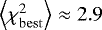$\text{left}<{\chi }_{\text{best}}^2\text{right}>\approx 2.9$, which is somewhat larger than for mock data (≈1), but still reasonably good.

Concerning the mean values used as observables, the Polaris Flare has a mean optical depth of $\langle {\tau }_{353}\rangle =\left(1.25\pm 0.05\right)\times {10}^{-5}$ and a mean temperatureof $\langle T_{\text{obs}}\rangle =17.5\pm 0.4$ K. Using the best fitting parameters from Table 4 we obtain optical depth maps with an average of $\langle {\tau }_{353}\rangle =\left(1.82\pm 0.05\right)\times {10}^{-5}$ over 60 realizations which is not fully consistent with the data value, as mentioned above for the ${\tau }_{353}/\langle {\tau }_{353}\rangle$ discrepancy. However the best fitting parameter for temperature is T_d = 17.5 ± 0.5 K which is exactly the same as in data with a width reflecting the data uncertainties.

The observables we used to extract the statistical properties of the Polaris Flare field are by themselves unable to constrain the γ₀ angle of the large-scale magnetic field on the LOS. However, the Planck Collaboration Int. XLIV (2016) analysis was able to fit the χ₀ and γ₀ angle is the southern Galactic cap and found an intrinsic polarization fraction of the gas of p_int ≈ 0.26. If we believe this latter value is true also in the Polaris Flare, then it is related to our fit as $p_0\approx p_{\text{int}}\langle {\cos }^2\gamma \rangle \approx p_{\text{int}}{\cos }^2{\gamma }_0$. We can thus constrain the γ₀ angle to be around 45°.

Fig. 8 Constraints (posterior probability contours and marginalized PDFs) on the statistical properties of the dust density and magnetic field for the Planck maps of the Polaris Flare. On the posterior probability contours, the filled dark and light blue regions respectively enclose 68.3% and 95.4% of the probability, and the black stars indicate the averages over the two-dimensional posterior PDFs. In the plots showing the marginalized posterior PDFs, the light blue regions enclose 68.3% of the probability, and the dashed blue lines indicate the averages over the posterior PDFs. The upper right plot displays the correlation matrix between the fitted parameters.

Fig. 9 Same as Fig. 7 with the same colour scales, but for model maps using the best fitting parameters to the Polaris Flare data.

Fig. 10 Comparison of the DFs extracted from the Planck Polaris Flare maps (black points) with the observables computed from simulations using the best fitting parameters (blue curves). The latter curves are averaged over 60 realizations, as describedin Sect. 4.2: the average is given by the central blue curve and the shaded bands give the 1σ and 2σ standard deviation in each bin.

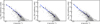Fig. 11 Comparison of the Im, Qm, and Um power spectra extracted from the Planck Polaris Flare maps (grey points representing the two-dimensional power spectra, and black dots representing the azimuthal averages in Fourier space) with the observables computed from simulations using the best fitting parameters (blue curves). The latter curves are averaged over 60 realizations as described in Sect 4.2: the average is given by the central blue curve and the narrow shaded bands give the 1σ and 2σ standard deviation in each bin.

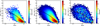Fig. 12 Two-dimensional distribution function of $\mathcal{S}$ and polarization fraction pMAS for the Polaris Flare maps (left), for the model maps using the best fitting parameters averaged over 60 realizations (middle), and residuals (right). The polarization angle dispersion function $\mathcal{S}$ is computed at a lag δ = 16′. The solid black line shows the mean $\mathcal{S}$ for each bin in pMAS and the dashed black line is a linear fit of that curve, restricted to bins in pMAS which contain at least 1% of the total number of points (120 × 120).

6 Discussion and summary

We have presented an analysis framework for maps of polarized thermal dust emission in the diffuse ISM aimed at constraining the statistical properties of the dust density and magnetic field responsible for this emission. Our framework rests on a set of synthetic models for the dust density and magnetic field, for which we precisely control the one- and two-point statistics, and on a least-squares analysis in which the space of parameters is explored via a MCMC method. The application of the method to Planck maps of the Polaris Flare molecular cloud leads to a spectral index of the turbulent component of the magnetic field β_B = 2.8 ± 0.2, which is in very good agreement with the findings of Planck Collaboration Int. XLIV (2016) and Vansyngel et al. (2017), who used a very different approach over a much larger fraction of the sky. The dust density field exhibits a much flatter spectrum, β_n = 1.7. This latter exponent is remarkably close to the Kolmogorov index for the velocity field in incompressible hydrodynamical turbulence, but this comparison should be taken with caution, as closer examination of the power spectrum of the model density field shows a spectral break with an exponent closer to 2.2 at the largest scales (k ≲ 1 pc⁻¹) while the smaller scales (k ≳ 1 pc⁻¹) have a 1.7 exponent¹⁰. It is, however, clear that the magnetic field power spectrum is much steeper, which underlines the role that the large scale magnetic field plays in the structure of polarized emission maps. We find that the fluctuation ratio of the dust density field and the ratio of turbulent-to-uniform magnetic field are both around unity. Finally, our analysis is able to give a constraint on the polarization fraction, p₀ ≈ 0.12, and on the depth of the Polaris Flare molecular cloud, d ≈ 13 pc, which is about half the transverse extent of the FoV, with ⟨n_H⟩≈ 40 cm⁻³. The good visual agreement between the Polaris Flare maps and model maps for the best-fitting parameters (Figs. 7and 9), and the excellent agreement between the two sets of maps for most of the observables used in the analysis (Figs. 10–12), all lead us to conclude that our fBm-based model, although limited, provides a reasonable description of the magnetized, turbulent, diffuse ISM.

In fact, it is quite remarkable to find such a good agreement with the data, considering the limitations of the model. First, it is statistically isotropic, and therefore cannot reproduce the interstellar filamentary structures observed at many scales and over a large range in column densities (see, e.g. Miville-Deschênes et al. 2010; Arzoumanian et al. 2011). Second, our model dust density and magnetic fields are completely uncorrelated, which is clearly not realistic, as it was found that there is a preferential relative orientation between structures of matter and magnetic field, both in molecular clouds (Planck Collaboration Int. XXXV 2016) and in the diffuse, high-latitude sky (Planck Collaboration Int. XXXII 2016; Planck Collaboration Int. XXXVIII 2016). The change in relative orientation, from mostly parallel to mostly perpendicular, as the total gas column density N_H increases, is also not reproducible with our fully-synthetic models. Third, it is now commonly acknowledged that two-point statistics such as power spectra are not sufficient to properly describe the structure of interstellar matter. Improving our synthetic models along these three directions will be the subject of future work.

For completeness, we have also looked into applying our MCMC approach based on fBm models to synthetic polarizationmaps built from a numerical simulation of MHD turbulence. We used simulation cubes¹¹ (Cho & Lazarian 2003; Burkhart et al. 2009, 2014), basing our choice on the simulation parameters, which seemed more or lessconsistent with the parameters found for the Polaris Flare data. We built simulated Stokes I, Q, and U maps using the same resolution and noise parameters, and launched the MCMC analysis on these simulated Stokes maps. It turns out that it is more difficult for the Markov chains to converge in this case than when applying the method to the Planck data. It is not yet completely clear why that is so, but we suspect that part of the reason may lie with the limited range of spatial scales over which the fields in the MHD simulation can be accurately described by scale-invariant processes. Indeed, while the fBm models exhibit power-law power spectra over the full range of accessible scales (basically one decade in our case), the MHD simulations are hampered by effects of numerical dissipation at small scales (possibly over nearly ten pixels), and the properties at large scales are dependent on the forcing, which is user-defined. The data, on theother hand, exhibit a much larger “inertial range”. In that respect, our fBm models, despite all their drawbacks, and despite the fact that they lack the physically realistic content of MHD simulations, provide a better framework for assessing the statistical properties of the Planck data than current MHD simulations can. Of course, this conclusion is based on just one simulation, and there would definitely be a point in applying the MCMC approach to assess various instances of MHD simulations with respect to the observational data, based on the same observables, but independently of the grid of fBm models. This project, however, is clearly beyond the scope of this paper.

Acknowledgements

We gratefully acknowledge fruitful discussions with S. Plaszczynski and O. Perdereau. This work was supported by the Programme National “Physique et Chimie du Milieu Interstellaire” (PCMI) of CNRS/INSU with INC/INP co-funded by CEA and CNES.

Appendix A Statistical properties of n_H models

A.1 Probability distribution function

The PDF f(n_H) of the density field n_H built using Eq. (4) derives from the Gaussian PDF of X, which in all generality has a mean ⟨X⟩ and variance ${\sigma }_X^2$. We thus have a log-normal PDF $$f(n_{\text{H}})=\frac{1}{\sqrt{2\pi }{\sigma }_X}\frac{X_r}{n_{\text{H}}}\exp \left\{-\frac{1}{2{\sigma }_X^2}{\left[X_r\ln \left(\frac{n_{\text{H}}}{n_0}\right)-\langle X\rangle \right]}^2\right\},$$(A.1)

which is defined for n_H > 0. Figure A.1 presents the distribution function of the n_H field¹² used to build Fig. 1, with the theoretical PDF expected from Eq. (A.1). We note that the distribution function for a single realisation over a finite grid such as the ones used here may deviate from the theoretical PDF, especially for large values of β_X, but the mean distribution function over a sufficiently large sample converges to the lognormal form (Eq. (A.1)).

A.2 Moments and fluctuation level

From Eq. (A.1), we may compute moments of any order p of the PDF of the total gas density n_H $$\text{nnleft}<n_{\text{H}}{}^p\text{right}>={\displaystyle {\int }_0^{\infty }{n}_{\text{H}}{}^p}f(n_{\text{H}})\text{\hspace{0.17em}d}{n}_{\text{H}}=n_0^p\exp \text{{left(}p\text{frac{left}<X\text{right}>\text{}}{X}_r+p^2\frac{{\sigma }_X^2}{2X_r^2}\text{right)}},$$(A.2)

which allows, in particular, to compute its mean value $$\text{nnleft}<n_{\text{H}}\text{right}>={\displaystyle {\int }_0^{\infty }{n}_{\text{H}}}f(n_{\text{H}})\text{\hspace{0.17em}d}{n}_{\text{H}}=n_0\exp \text{{left(frac{left}<X\text{right}>\text{}}{X}_r+\frac{{\sigma }_X^2}{2X_r^2}\text{right)}},$$(A.3)

as well as its variance $${\sigma }_{n_{\text{H}}}^2=n_0^2\exp \text{{left(}2\text{frac{left}<X\text{right}>\text{}}{X}_r\text{right)}}\left[\exp \left(\frac{2{\sigma }_X^2}{X_r^2}\right)-\exp \left(\frac{{\sigma }_X^2}{X_r^2}\right)\right].$$(A.4)

The density fluctuation level, which is one of the parameters of our model, is therefore $$y_n=\frac{{\sigma }_{n_{\text{H}}}}{\langle n_{\text{H}}\rangle }=\sqrt{2}\exp \left(\frac{{\sigma }_X^2}{4X_r^2}\right){\left[\sinh \left(\frac{{\sigma }_X^2}{2X_r^2}\right)\right]}^{1/2}.$$(A.5)

For instance, the n_H field whose distribution function is shown in Fig. A.1 has values ranging from 0.3 cm⁻³ to 880 cm⁻³, with a mean and standard deviation of 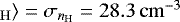$\langle n_{\text{H}}\rangle ={\sigma }_{n_{\text{H}}}=28.3{\text{cm}}^{-3}$, resulting in the desired fluctuation level y_n = 1.

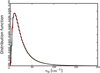Fig. A.1 Distribution function of the synthetic field nH used for Fig. 1 (black histogram). The red curve shows the theoretical probability distribution function f(nH) for the chosen set of parameters.

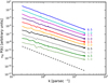Fig. A.2 Power spectra $P_{n_{\text{H}}}(k)$ of synthetic nH fields obtained by exponentiation of a 120 × 120 × 120 pixels fractional Brownian motion with spectral index βX = 3. The fluctuation levels yn are specified next to each curve, and the original field’s power spectrum $P_{n_{\text{H}}}(k)$ is represented as a dashed line.

Power spectra

Figure A.2 shows the azimuthally-averaged power spectra of n_H fields obtained through Eq. (4), from a 120 × 120 × 120 pixels fractional Brownian motion X with spectral index β_X = 3, for various fluctuation levels y_n. The spectra were normalized differently so as to allow comparison between them.

The power-law behaviour is apparent, even at large fluctuation levels, but the spectral index decreases (i.e., the spectra flatten) as the fluctuation level increases. This is quantified in Fig. A.3, which shows the differences β_n − β_X between the spectral indices of the original fBm field X and that of the model density field n_H. The power spectra of the latter are indeed flatter than the original ones (β_n < β_X), with differences that may become large when β_X is low, but remain negligible for higher β_X. We interpret this trend as the exponentiation process amplifying the two-point differences X(r+ δ) − X(r), for small separations ||δ ||, that exist in the original field when β_X is low, leading to an increase of the small-scale power in the model n_H field, i.e. β_n < β_X. This effect is all the more important when exponentiation stretches these field differences more strongly, i.e. when y_n increases. On the other hand, for high β_X, the fBm fields are much smoother, so the exponentiation process has little impact on these two-point statistics at small scales, leading to β_n ≃ β_X. We note that at low fluctuation levels (y_n ≤ 0.3), the differences are smaller than 0.1 for all values of β_X.

Fig. A.3 Evolution of the differences βn − βX between the spectral indices of the original fBm field X and that of the model density field nH with fluctuation level yn. Each point corresponds to the mean of 20 realisations of the model density field nH, and the error bars represent the standard deviation of the fitted spectral indices βn and fluctuation levels yn.

Appendix B: Likelihood terms

B.1 D² terms for mean values

The first term in Eq. (25) is given by $$D_{\mu }^2=\frac{{\left(\langle {\tau }_{353}^{\text{m}}\rangle -\langle {\tau }_{353}^{\text{d}}\rangle \right)}^2}{{\sigma }_{\langle {\tau }_{353}^{\text{m}}\rangle }^2+{\sigma }_{\langle {\tau }_{353}^{\text{d}}\rangle }^2}+\frac{{\left(\langle T_{\text{obs}}\rangle -T_{\text{d}}\right)}^2}{{\sigma }_{\langle T_{\text{obs}}\rangle }^2}.$$(B.1)

The mean value of the optical depth τ₃₅₃ is evaluated on the simulated ${\tau }_{353}^{\text{m}}$ and Planck data ${\tau }_{353}^{\text{d}}$ maps. These are compared through a standard χ² test. The denominator includes the uncertainty ${\sigma }_{\langle {\tau }_{353}^{\text{d}}\rangle }$ on the mean ${\tau }_{353}^{\text{d}}$ value propagated from the uncertainty map provided by the Planck collaboration (Planck Collaboration XI 2014), and the uncertainty ${\sigma }_{\langle {\tau }_{353}^{\text{m}}\rangle }$ coming from the conversion factor ${\sigma }_{353}\left(N_{\text{H}}\right)$ used to build the simulated map (Planck Collaboration XI 2014).

In the second term, $\langle T_{\text{obs}}\rangle$ is the mean value of the temperature map T_obs from Planckdata, and ${\sigma }_{\langle T_{\text{obs}}\rangle }$ represents the uncertainty on the averaged value propagated from the uncertainty map provided by the Planck collaboration. T_d is directly the model parameter for the dust temperature.

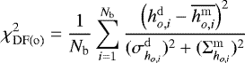
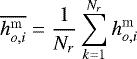
B.2 D² terms for distribution functions

For a given observable map o, we compute its DF over an ensemble of N_b bins¹³. When considering the Planck data, we write this DF as $h_{o,i}^{\text{d}}$, where i is the bin number, and we estimate the uncertainty on the value of the DF in bin i through the associated Poisson noise ${\sigma }_{h_{o,i}^{\text{d}}}$. When considering the model, we write $h_{o,i}^{\text{m}}$ and ${\sigma }_{h_{o,i}^{\text{m}}}$ to be respectively the bin value and the Poisson noise of the DF in bin i, independently for each of the N_r = 60 model realizations.

The contribution $D_{\text{DF}(o)}^2$ of the observable’s DF to the total D² in Eq. (25) is then built as an average over the N_b bins 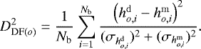$$D_{\text{DF}(o)}^2=\frac{1}{N_{\text{b}}}{\sum }_{i=1}^{N_{\text{b}}}\frac{{\left(h_{o,i}^{\text{d}}-h_{o,i}^{\text{m}}\right)}^2}{{({\sigma }_{h_{o,i}^{\text{d}}})}^2+{({\sigma }_{h_{o,i}^{\text{m}}})}^2}.$$(B.2)

The sum is normalized to the number of bins so that $D_{\text{DF}(o)}^2$ is less sensitive to the binning choice and the map noise. If the model fits the data correctly as far as the DF of observable o is concerned, then $D_{\text{DF}(o)}^2$ is minimum.

This quantity is different from a standard χ² test as it compares data with one random¹⁴ realisation for a given set of model parameters, and this comparison is repeated and averaged N_r times. A standard χ² test would compare data with a model prediction that would be the average of the random realizations (see Eq (C.3) in Appendix C). The latter could not be used in our MCMC analysis due to the mathematical relation between the power spectrum of the map and the variance in each bin of the DF: with steep power spectra (high values of the spectral index β), only the few large-scale modes effectively contribute to the power, leading to a large variance in each DF bin¹⁵. Thus the χ² test tends to favour these large values of β, as they yield large denominators and thus allow for a “good” fit. This drives the fit towards a region of parameter space yielding mean DFs that fit the data well but with a huge dispersion: one realization of such a model gives a DF with bin values highly scattered even though the data DF is quite smooth. This means that the data cannot reasonably be interpreted as a random realization using these parameter values, and explains why we had to switch to the D² function, which directly compares data with one model random realization. In this fashion, we are able to reach the region of parameter space correctly describing the data.

B.3 D² terms for power spectra

For a given observable map o, we first compute its two-dimensional power spectrum $$P_o(k)={\left|\text{\hspace{0.17em}widetilde}o(k)\right|}^2$$(B.3)

then average these within ${N^{\prime }}_{\text{b}}$ annuli in Fourier space, centred on a set of wavenumbers $\left\{k_i\right\}$. We write $P_{o,i}^{\text{d}}$ for this azimuthal average in bin i when considering the Planck data, and $P_{o,i}^{\text{m}}$ when considering model fields. The uncertainties affecting these quantities strongly depend on the number N_i of wavevectors k_n in each bin. The best estimate for the standard deviation ${\sigma }_{P_{o,i}^{\text{d}}}$ of the power spectrum of the data is $${\sigma }_{P_{o,i}^{\text{d}}}=t_{N_i}\sqrt{\frac{1}{N_i\left(N_i-1\right)}{\sum }_{n=1}^{N_i}{\left[P_o^d(k_n)-P_{o,i}^d\right]}^2}$$(B.4)

where the factor t_N is the Student coefficient. We thus obtain the best estimate of the true standard deviation in bins with only a few modes (i.e. at large scale). The standard deviation ${\sigma }_{P_{o,i}^{\text{m}}}$ for the 60 model realizations is computed in the same way as for data.

The contribution $D_{P(o)}^2$ of the observable’s power spectrum to the total D² in Eq. (25) is then computed as an average over the ${N^{\prime }}_{\text{b}}$ bins¹⁶ in wavenumberspace, 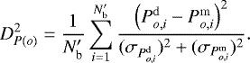$$D_{P(o)}^2=\frac{1}{{N^{\prime }}_{\text{b}}}{\sum }_{i=1}^{{N^{\prime }}_{\text{b}}}\frac{{\left(P_{o,i}^{\text{d}}-P_{o,i}^{\text{m}}\right)}^2}{{({\sigma }_{P_{o,i}^{\text{d}}})}^2+{({\sigma }_{P_{o,i}^{\text{m}}})}^2}.$$(B.5)

B.4: D² term for the $\left\{\mathcal{S},p_{\text{MAS}}\right\}$ anti-correlation

To use the $\left\{\mathcal{S},p_{\text{MAS}}\right\}$ anti-correlation (Planck Collaboration Int. XIX 2015; Planck Collaboration Int. XX 2015), we compute the joint distribution function of the $\mathcal{S}$ and p_MAS maps, which we write $h_{ij}^{\text{d}}$ and $h_{ij}^{\text{m}}$ for the Planck data and model maps respectively, with 1 ≤ i ≤ N_b,1 and 1 ≤ j ≤ N_b,2 the binning scheme used for the two maps. The standard deviations ${\sigma }_{ij}^{\text{d}}$ and ${\sigma }_{ij}^{\text{m}}$ are defined in the same way as for the one-dimensional DFs in Sect. B.2, and the contribution $D_{\mathcal{S}-p_{\text{MAS}}}^2$ to the total D² is then $$D_{\mathcal{S}-p_{\text{MAS}}}^2=\frac{1}{N_{\text{b},\text{tot}}}{\sum }_{i=1}^{N_{\text{b},\text{1}}}{\sum }_{j=1}^{N_{\text{b},\text{2}}}\frac{{\left(h_{ij}^{\text{d}}-h_{ij}^{\text{m}}\right)}^2}{{({\sigma }_{ij}^{\text{d}})}^2+{({\sigma }_{ij}^{\text{m}})}^2}.$$(B.6)

In this expression, we note that the total number N_b,tot of two-dimensional bins considered is less than the product N_b,1N_b,2 of the number of bins in each dimension, which we set to N_b,1 = N_b,2 = 50. The reason for this is that we discard the empty bins and those with a signal-to-noise ratio below three¹⁷. We thus keep only the significantly populated bins that can drive the fit and contribute to the total D².

Appendix C: Goodness-of-fit

To assess the goodness of the fit, we use an a posteriori χ² test, which we define as $${\chi }^2=\frac{1}{N_o}\left[{\chi }_{\mu }^2+{\sum }_o{\chi }_{\text{DF}(o)}^2+{\sum }_o{\chi }_{P(o)}^2+{\chi }_{\mathcal{S}-p_{\text{MAS}}}^2\right]$$(C.1)

with N_o = 13 the total number of observables. Each term is a χ² test comparing data with the mean of the N_r = 60 realisations. The first term from Eq (C.1) is $${\chi }_{\mu }^2=\frac{{\left(\overline{\langle {\tau }_{353}^{\text{m}}\rangle }-\langle {\tau }_{353}^{\text{d}}\rangle \right)}^2}{{\Sigma }_{\langle {\tau }_{353}^{\text{m}}\rangle }^2+{\sigma }_{\langle {\tau }_{353}^{\text{d}}\rangle }^2}+\frac{{\left(\langle T_{\text{obs}}\rangle -T_{\text{d}}\right)}^2}{{\sigma }_{\langle T_{\text{obs}}\rangle }^2}$$(C.2)

where $\overline{\langle {\tau }_{353}^{\text{m}}\rangle }$ is the ensemble average over the 60 model realisations of the (spatial) mean of the optical depth. In the following, the brackets stand for an average on the pixels while the upper bar represents the average over the N_r realisations. The ${\Sigma }_{\langle {\tau }_{353}^{\text{m}}\rangle }^2$ quantity is the variance of $\langle {\tau }_{353}^{\text{m}}\rangle$ over the N_r realisations (capital Σ denotes the variance over the random realisations).

The second term is $${\chi }_{\text{DF}(\text{o})}^2=\frac{1}{N_{\text{b}}}{\sum }_{i=1}^{N_{\text{b}}}\frac{{\left(h_{o,i}^{\text{d}}-\overline{h_{o,i}^{\text{m}}}\right)}^2}{{({\sigma }_{h_{o,i}}^{\text{d}})}^2+{({\Sigma }_{h_{o,i}}^{\text{m}})}^2}$$(C.3)

where $$\overline{h_{o,i}^{\text{m}}}=\frac{1}{N_r}{\sum }_{k=1}^{N_r}{h}_{o,i}^{\text{m}}$$(C.4)

is the ensemble average of the i^th bin of the DF for the observable o, over the N_r = 60 model realizations, and ${({\Sigma }_{h_{o,i}}^{\text{m}})}^2$ is the associated variance. We note that while $D_{\text{DF}(\text{o})}^2$ in Eq. (B.2) is the average of the observable χ², ${\chi }_{\text{DF}(\text{o})}^2$ is the χ² of the averaged observable.

The third term is 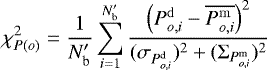$${\chi }_{P(o)}^2=\frac{1}{{N^{\prime }}_{\text{b}}}{\sum }_{i=1}^{{N^{\prime }}_{\text{b}}}\frac{{\left(P_{o,i}^{\text{d}}-\overline{P_{o,i}^{\text{m}}}\right)}^2}{{({\sigma }_{P_{o,i}^{\text{d}}})}^2+{({\Sigma }_{P_{o,i}^{\text{m}}})}^2}$$(C.5)

where $\overline{P_{o,i}^{\text{m}}}$ is the averaged power spectrum in bin i and ${({\Sigma }_{P_{o,i}^{\text{m}}})}^2$ its variance.

Finally, the fourth term is 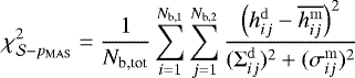$${\chi }_{\mathcal{S}-p_{\text{MAS}}}^2=\frac{1}{N_{\text{b},\text{tot}}}{\sum }_{i=1}^{N_{\text{b},\text{1}}}{\sum }_{j=1}^{N_{\text{b},\text{2}}}\frac{{\left(h_{ij}^{\text{d}}-\overline{h_{ij}^{\text{m}}}\right)}^2}{{({\Sigma }_{ij}^{\text{d}})}^2+{({\sigma }_{ij}^{\text{m}})}^2}$$(C.6)

with the same notation conventions as above.

To quantify the goodness of fit, once the MCMC procedure has converged, we perform 100 fits for the set of best fitting parameters, each of these fits comprising 60 model realizations and providing a value of the χ² quantity defined in Eq. (C.1). The average of these 100 χ² values¹⁸ is listed as $\text{left}<{\chi }_{\text{best}}^2\text{right}>$ in Tables 3 and 4.

References

All Tables

All Figures

	Fig. 1 Total gas column density NH, derived froma synthetic density field nH built by exponentiation of a fBm field with spectral index βX = 2.6 and size 120 × 120 × 120 pixels. The volume density fluctuation level is yn = 1, and the column density fluctuation level is $y_{N_{\text{H}}}\simeq 0.25$.
In the text

Fig. 2 Synthetic magnetic field B built using Eq. (8). The spectral index of the vector potential is βA = 5 and the size of the cubes is 120 × 120 × 120 pixels, corresponding to 30 pc on each side. Shown are two-dimensional slices through the cubes of the components Bx (top), By (middle), and Bz (bottom). The ratio of the fluctuations of the turbulent component Bt to the norm of the uniform component B0 is yB =1 in this particular case, with angles χ0 = γ0 = 0°.

In the text

Fig. 3 Distribution functions of the components Bx, By, and Bz of a model magnetic field B = B0 + Bt built on a grid 120 × 120 × 120 pixels using Eq. (8) with βA = 5, and a mean, large-scale magnetic field B0 defined by the angles χ0 = 0° and γ0 = 60°, and a norm B0 = 50 μG such that the fluctuation level is yB = 0.1. The vertical lines represent the projected values of the large scale magnetic field B0x = B0 sinχ0 cosγ0, B0y = −B0 cosχ0 cosγ0 and B0z = B0 sinγ0. See Fig. 14 in Planck Collaboration Int. XX (2015) for the definition of angles.

In the text

Fig. 4 Powerspectra of the components Bx, By and Bz of a model magnetic field B = B0 + Bt built on a grid 120 × 120 × 120 pixels using Eq. (8) with βA = 3 (different shades of blue for the three components) and βA = 5 (different shades of red for the three components). The power spectra are normalized differently so as to allow comparison between them. The fitted power-laws shown as solid lines yield spectral indices βB = 1 and βB = 3, in agreement with Eq. (11). These are the power spectra of the same particular realizations shown in Fig. 2.

In the text

Fig. 5 Left column row: example maps (from top to bottom: total intensity Im on a logarithmic scale, Stokes Qm, and Stokes Um) from simulation A (see Sect. 5 and Table 3). Right column: corresponding power spectra. The grey points represent the two-dimensional power spectra, while the black dots represent the azimuthal averages in Fourier space in a set of wavenumber bins, and the blue line is a power-law fit to the black points.

In the text

Fig. 6 Constraints (posterior probability contours and marginalized PDFs) on the statistical properties of the dust density and magnetic field for the simulation A maps. On the posterior probability contours, the filled dark and light blue regions respectively enclose 68.3% and 95.4% of the probability, the black stars indicate the averages over the two-dimensional posterior PDFs, and the red circles indicate the input values for the simulation. In the plots showing the marginalized posterior PDFs, the light blue regions enclose 68.3% of the probability, the dashed blue lines indicate the averages over the posterior PDFs, and the solid red lines indicate the input values for the simulation. The upper right plot displays the correlation matrix between the fitted parameters.

In the text

Fig. 7 Planck 353 GHz maps of the Polaris Flare molecular cloud. The top row shows, from left to right, the total intensity I353 on a logarithmic scale, the Stokes Q353 map and the Stokes U353 map, while the bottom row shows the polarization fraction pMAS, the polarization angle ψ, and the polarization angle dispersion function $\mathcal{S}$. The τ353 and Tobs maps have the same aspects as the I353 map but with their own scales.

In the text

Fig. 8 Constraints (posterior probability contours and marginalized PDFs) on the statistical properties of the dust density and magnetic field for the Planck maps of the Polaris Flare. On the posterior probability contours, the filled dark and light blue regions respectively enclose 68.3% and 95.4% of the probability, and the black stars indicate the averages over the two-dimensional posterior PDFs. In the plots showing the marginalized posterior PDFs, the light blue regions enclose 68.3% of the probability, and the dashed blue lines indicate the averages over the posterior PDFs. The upper right plot displays the correlation matrix between the fitted parameters.

In the text

	Fig. 9 Same as Fig. 7 with the same colour scales, but for model maps using the best fitting parameters to the Polaris Flare data.
In the text

	Fig. 10 Comparison of the DFs extracted from the Planck Polaris Flare maps (black points) with the observables computed from simulations using the best fitting parameters (blue curves). The latter curves are averaged over 60 realizations, as describedin Sect. 4.2: the average is given by the central blue curve and the shaded bands give the 1σ and 2σ standard deviation in each bin.
In the text

Fig. 11 Comparison of the Im, Qm, and Um power spectra extracted from the Planck Polaris Flare maps (grey points representing the two-dimensional power spectra, and black dots representing the azimuthal averages in Fourier space) with the observables computed from simulations using the best fitting parameters (blue curves). The latter curves are averaged over 60 realizations as described in Sect 4.2: the average is given by the central blue curve and the narrow shaded bands give the 1σ and 2σ standard deviation in each bin.

In the text

Fig. 12 Two-dimensional distribution function of $\mathcal{S}$ and polarization fraction pMAS for the Polaris Flare maps (left), for the model maps using the best fitting parameters averaged over 60 realizations (middle), and residuals (right). The polarization angle dispersion function $\mathcal{S}$ is computed at a lag δ = 16′. The solid black line shows the mean $\mathcal{S}$ for each bin in pMAS and the dashed black line is a linear fit of that curve, restricted to bins in pMAS which contain at least 1% of the total number of points (120 × 120).

In the text

	Fig. A.1 Distribution function of the synthetic field nH used for Fig. 1 (black histogram). The red curve shows the theoretical probability distribution function f(nH) for the chosen set of parameters.
In the text

	Fig. A.2 Power spectra $P_{n_{\text{H}}}(k)$ of synthetic nH fields obtained by exponentiation of a 120 × 120 × 120 pixels fractional Brownian motion with spectral index βX = 3. The fluctuation levels yn are specified next to each curve, and the original field’s power spectrum $P_{n_{\text{H}}}(k)$ is represented as a dashed line.
In the text

	Fig. A.3 Evolution of the differences βn − βX between the spectral indices of the original fBm field X and that of the model density field nH with fluctuation level yn. Each point corresponds to the mean of 20 realisations of the model density field nH, and the error bars represent the standard deviation of the fitted spectral indices βn and fluctuation levels yn.
In the text

References

- Alina, D., Montier, L., Ristorcelli, I., et al. 2016, A&A, 595, A57 [NASA ADS] [CrossRef] [EDP Sciences] [Google Scholar]
- André, P., Men’shchikov, A., Bontemps, S., et al. 2010, A&A, 518, L102 [NASA ADS] [CrossRef] [EDP Sciences] [Google Scholar]
- Arzoumanian, D., André, P., Didelon, P., et al. 2011, A&A, 529, L6 [Google Scholar]
- Benoît, A., Ade, P., Amblard, A., et al. 2004, A&A, 424, 571 [NASA ADS] [CrossRef] [EDP Sciences] [Google Scholar]
- Beresnyak, A. 2014, ApJ, 784, L20 [NASA ADS] [CrossRef] [Google Scholar]
- Bierman, E. M., Matsumura, T., Dowell, C. D., et al. 2011, ApJ, 741, 81 [NASA ADS] [CrossRef] [Google Scholar]
- Brooks, S., Gelman, A., Jones, G. L., & Meng, X. L. 2011, Handbook of Markov Chain Monte Carlo (Boca Raton: Chapman & Hall/CRC) [Google Scholar]
- Brunt, C. M., & Heyer, M. H. 2002, ApJ, 566, 289 [NASA ADS] [CrossRef] [Google Scholar]
- Burkhart, B., & Lazarian, A. 2016, ApJ, 827, 26 [NASA ADS] [CrossRef] [Google Scholar]
- Burkhart, B., Falceta-Gonçalves, D., Kowal, G., & Lazarian, A. 2009, ApJ, 693, 250 [NASA ADS] [CrossRef] [Google Scholar]
- Burkhart, B., Lazarian, A., Leão, I. C., de Medeiros, J. R., & Esquivel, A. 2014, ApJ, 790, 130 [NASA ADS] [CrossRef] [Google Scholar]
- Chandrasekhar, S., & Fermi, E. 1953, ApJ, 118, 113 [NASA ADS] [CrossRef] [Google Scholar]
- Cho, J., & Lazarian, A. 2003, MNRAS, 345, 325 [NASA ADS] [CrossRef] [Google Scholar]
- Correia, C., Lazarian, A., Burkhart, B., Pogosyan, D., & De Medeiros J. R. 2016, ApJ, 818, 118 [NASA ADS] [CrossRef] [Google Scholar]
- Dotson, J. L., Vaillancourt, J. E., Kirby, L., et al. 2010, ApJS, 186, 406 [NASA ADS] [CrossRef] [Google Scholar]
- Falceta-Gonçalves, D., Lazarian, A., & Kowal, G. 2008, ApJ, 679, 537 [NASA ADS] [CrossRef] [Google Scholar]
- Falconer, K. 1990, Fractal Geometry: Mathematical Foundations and Applications (Chichester: John Wiley & Sons) [Google Scholar]
- Falgarone, E., Panis, J.-F., Heithausen, A., et al. 1998, A&A, 331, 669 [NASA ADS] [Google Scholar]
- Fissel, L. M., Ade, P. A. R., Angilè, F. E., et al. 2016, ApJ, 824, 134 [NASA ADS] [CrossRef] [Google Scholar]
- Gelman, A., & Rubin, D. B. 1992, Statist. Sci., 7, 457 [NASA ADS] [CrossRef] [Google Scholar]
- Górski, K. M., Hivon, E., Banday, A. J., et al. 2005, ApJ, 622, 759 [NASA ADS] [CrossRef] [Google Scholar]
- Hamann, J., Hannestad, S., Raffelt, G. G., & Wong, Y. Y. Y. 2007, JCAP, 8, 021 [NASA ADS] [CrossRef] [Google Scholar]
- Haverkorn, M., Brown, J. C., Gaensler, B. M., & McClure-Griffiths, N. M. 2008, ApJ, 680, 362 [NASA ADS] [CrossRef] [Google Scholar]
- Hennebelle, P. 2013, A&A, 556, A153 [NASA ADS] [CrossRef] [EDP Sciences] [Google Scholar]
- Hennebelle, P., & Falgarone, E. 2012, A&ARv, 20, 55 [NASA ADS] [CrossRef] [Google Scholar]
- Hennebelle, P., & Iffrig, O. 2014, A&A, 570, A81 [NASA ADS] [CrossRef] [EDP Sciences] [Google Scholar]
- Hennebelle, P., Banerjee, R., Vázquez-Semadeni, E., Klessen, R. S., & Audit, E. 2008, A&A, 486, L43 [NASA ADS] [CrossRef] [EDP Sciences] [Google Scholar]
- Hildebrand, R. H., Kirby, L., Dotson, J. L., Houde, M., & Vaillancourt, J. E. 2009, ApJ, 696, 567 [NASA ADS] [CrossRef] [Google Scholar]
- Hily-Blant, P.,& Falgarone, E. 2009, A&A, 500, L29 [NASA ADS] [CrossRef] [EDP Sciences] [Google Scholar]
- Hull, C. L. H., Plambeck, R. L., Kwon, W., et al. 2014, ApJS, 213, 13 [NASA ADS] [CrossRef] [Google Scholar]
- Inutsuka, S.-i., Inoue, T., Iwasaki, K., & Hosokawa, T. 2015, A&A, 580, A49 [NASA ADS] [CrossRef] [EDP Sciences] [Google Scholar]
- Jaffe, T. R., Leahy, J. P., Banday, A. J., et al. 2010, MNRAS, 401, 1013 [NASA ADS] [CrossRef] [Google Scholar]
- Jansson, R., & Farrar, G. R. 2012, ApJ, 761, L11 [NASA ADS] [CrossRef] [Google Scholar]
- Koch, P. M., Tang, Y.-W., Ho, P. T. P., et al. 2014, ApJ, 797, 99 [NASA ADS] [CrossRef] [Google Scholar]
- Levrier, F., Falgarone, E., & Viallefond, F. 2006, A&A, 456, 205 [NASA ADS] [CrossRef] [EDP Sciences] [Google Scholar]
- Matthews, B. C., McPhee, C. A., Fissel, L. M., & Curran, R. L. 2009, ApJS, 182, 143 [NASA ADS] [CrossRef] [Google Scholar]
- Miville-Deschênes, M.-A., Levrier, F., & Falgarone, E. 2003, ApJ, 593, 831 [NASA ADS] [CrossRef] [Google Scholar]
- Miville-Deschênes, M.-A., Ysard, N., Lavabre, A., et al. 2008, A&A, 490, 1093 [NASA ADS] [CrossRef] [EDP Sciences] [Google Scholar]
- Miville-Deschênes, M.-A., Martin, P. G., Abergel, A., et al. 2010, A&A, 518, L104 [NASA ADS] [CrossRef] [EDP Sciences] [Google Scholar]
- Montier, L., Plaszczynski, S., Levrier, F., et al. 2015a, A&A, 574, A135 [NASA ADS] [CrossRef] [EDP Sciences] [Google Scholar]
- Montier, L., Plaszczynski, S., Levrier, F., et al. 2015b, A&A, 574, A136 [NASA ADS] [CrossRef] [EDP Sciences] [Google Scholar]
- O’Dea, D. T., Clark, C. N., Contaldi, C. R., & MacTavish, C. J. 2012, MNRAS, 419, 1795 [NASA ADS] [CrossRef] [Google Scholar]
- Panopoulou, G. V., Psaradaki, I., & Tassis, K. 2016, MNRAS, 462, 1517 [NASA ADS] [CrossRef] [Google Scholar]
- Perez, J. C., Mason, J., Boldyrev, S., & Cattaneo, F. 2012, Phys. Rev. X, 2, 041005 [Google Scholar]
- Planck Collaboration I. 2016, A&A, 594, A1 [NASA ADS] [CrossRef] [EDP Sciences] [Google Scholar]
- Planck Collaboration XI. 2014, A&A, 571, A11 [NASA ADS] [CrossRef] [EDP Sciences] [Google Scholar]
- Planck Collaboration Int. XIX. 2015, A&A, 576, A104 [NASA ADS] [CrossRef] [EDP Sciences] [Google Scholar]
- Planck Collaboration Int. XX. 2015, A&A, 576, A105 [NASA ADS] [CrossRef] [EDP Sciences] [Google Scholar]
- Planck Collaboration Int. XXX. 2016, A&A, 586, A133 [NASA ADS] [CrossRef] [EDP Sciences] [Google Scholar]
- Planck Collaboration Int. XXXII. 2016, A&A, 586, A135 [NASA ADS] [CrossRef] [EDP Sciences] [Google Scholar]
- Planck Collaboration Int. XXXV. 2016, A&A, 586, A138 [NASA ADS] [CrossRef] [EDP Sciences] [Google Scholar]
- Planck Collaboration Int. XXXVIII. 2016, A&A, 586, A141 [NASA ADS] [CrossRef] [EDP Sciences] [Google Scholar]
- Planck Collaboration Int. XLIV. 2016, A&A, 596, A105 [NASA ADS] [CrossRef] [EDP Sciences] [Google Scholar]
- Plaszczynski, S., Montier, L., Levrier, F., & Tristram, M. 2014, MNRAS, 439, 4048 [NASA ADS] [CrossRef] [Google Scholar]
- Ponthieu, N., Macías-Pérez, J. F., Tristram, M., et al. 2005, A&A, 444, 327 [NASA ADS] [CrossRef] [EDP Sciences] [Google Scholar]
- Schlafly, E. F., Green, G., Finkbeiner, D. P., et al. 2014, ApJ, 786, 29 [NASA ADS] [CrossRef] [Google Scholar]
- Seifried, D., & Walch, S. 2015, MNRAS, 452, 2410 [NASA ADS] [CrossRef] [Google Scholar]
- Soler, J. D., Hennebelle, P., Martin, P. G., et al. 2013, ApJ, 774, 128 [NASA ADS] [CrossRef] [Google Scholar]
- Soler, J. D., Alves, F., Boulanger, F., et al. 2016, A&A, 596, A93 [NASA ADS] [CrossRef] [EDP Sciences] [Google Scholar]
- Stutzki, J., Bensch, F., Heithausen, A., Ossenkopf, V., & Zielinsky, M. 1998, A&A, 336, 697 [NASA ADS] [Google Scholar]
- Vaillancourt, J. E., & Matthews, B. C. 2012, ApJS, 201, 13 [NASA ADS] [CrossRef] [Google Scholar]
- Vansyngel, F., Boulanger, F., Ghosh, T., et al. 2017, A&A, 603, A62 [NASA ADS] [CrossRef] [EDP Sciences] [Google Scholar]
- Ward-Thompson, D., Sen, A. K., Kirk, J. M., & Nutter, D. 2009, MNRAS, 398, 394 [NASA ADS] [CrossRef] [Google Scholar]
Planck (http://www.esa.int/Planck) is a project of the European Space Agency (ESA) with instruments provided by two scientific consortia funded by ESA member states and led by principal investigators from France and Italy, telescope reflectors provided through a collaboration between ESA and a scientific consortium led and funded by Denmark, and additional contributions from NASA (USA).
In all generality, several spectral indices may be defined, as one may consider the power spectrum of any one of the three cartesian components of Bt, or of the modulus |Bt|. Assuming that Bt is isotropic, which we will, all of these spectral indices are identical.
Throughout this paper, for any field F
the notation  represents its Fourier transform.
We do not consider an ordered random or striated random component of the field (Jaffe et al. 2010; Jansson & Farrar 2012), which we justify with the smallness of the field-of-view considered.
Not to be confused with the corresponding position angle χ0 of the uniform component of the magnetic field B0.
A more recent determination of the distance to the Polaris Flare places it at 350–400 pc (Schlafly et al. 2014). For the demonstration of the method presented here, this is not a critical issue, as the power-law power spectra underline self-similar behaviours, so that a change of the distance can be compensated by a change in pixel size.
The conversion factor is given for a map of NH at a resolution of 30′. Thus, before applying it pixel by pixel, we smooth the simulated NH map to 30′ resolution, apply the conversion, then resample the resulting τ353 map at the original resolution.
And after removing the burn-in phase, which is quite short in our case (≲30% of the chain lengths in general).
Incidentally, from the Planck maps, we can measure the spectral index of the total intensity for the Polaris Flare to be βI = 2.84 ± 0.10, in excellent agreement with the measurement by Stutzki et al. (1998) on CO integrated emission at a similar angular resolution.
In that case, ⟨X⟩ = 0,
,
Xr = 1.2, and
n0 = 20 cm−3.
We set Nb = 50 for the 120 × 120 pixel maps.
We remind the reader that the randomness comes from the fBm itself and the noise addition to the Stokes maps.
This is akin to the cosmic variance problem in cosmology.
To have reliable and smooth power spectra with 120 × 120 pixel maps, we set initially  but later cut off wavenumbers larger than kmax = 2π∕(3 × 15′), which corresponds to scales smaller than three beam sizes. Indeed, for bins
ki > kmax
the power spectrum is completely washed out by the beam convolution (see Fig. 5) and contains no information about the underlying interesting parameters. This uninformative part is thus removed from
but later cut off wavenumbers larger than kmax = 2π∕(3 × 15′), which corresponds to scales smaller than three beam sizes. Indeed, for bins
, and thus
.
i.e., bins where  ,
, or
Each simulation is a random realization of the fBm and the noise, then the χ2 values have an intrinsic dispersion even when compiling 60 simulations. To check the agreement with data, we thus average 100 computations of the best χ2 value.