CO enhancement by magnetohydrodynamic waves

R. Skalidis; K. Gkimisi; K. Tassis; G. V. Panopoulou; V. Pelgrims; A. Tritsis; P. F. Goldsmith

doi:10.1051/0004-6361/202345880

Home

All issues

Volume 673 (May 2023)

A&A, 673 (2023) A76

Full HTML

Open Access

Issue		A&A Volume 673, May 2023


Article Number		A76
Number of page(s)		15
Section		Interstellar and circumstellar matter
DOI		https://doi.org/10.1051/0004-6361/202345880
Published online		10 May 2023

A&A 673, A76 (2023)

Striations in the Polaris Flare^★

R. Skalidis¹, K. Gkimisi²^,3, K. Tassis²^,3, G. V. Panopoulou⁴, V. Pelgrims²^,3, A. Tritsis⁵ and P. F. Goldsmith⁶

¹ Owens Valley Radio Observatory, California Institute of Technology, MC 249-17, Pasadena, CA 91125, USA
e-mail: skalidis@caltech.edu
² Department of Physics & ITCP, University of Crete, 70013 Heraklion, Greece
e-mail: tassis@physics.uoc.gr
³ Institute of Astrophysics, Foundation for Research and Technology-Hellas, Vasilika Vouton, 70013 Heraklion, Greece
⁴ Department of Physics, University of Cyprus, 1 Panepistimiou Avenue, 2109 Aglantzia, Nicosia, Cyprus
⁵ Institute of Physics, Laboratory of Astrophysics, École Polytechnique Fédérale de Lausanne (EPFL), Observatoire de Sauverny, 1290 Versoix, Switzerland
⁶ Jet Propulsion Laboratory, California Institute of Technology, 4800 Oak Grove Drive, Pasadena, CA 91109-8099, USA

Received: 10 January 2023
Accepted: 1 March 2023

Abstract

Context. The formation of molecular gas in interstellar clouds is a slow process, but can be enhanced by gas compression. Magneto-hydrodynamic (MHD) waves can create compressed quasi-periodic linear structures, referred to as striations. Striations are observed at the column densities at which the transition from atomic to molecular gas takes place.

Aims. We explore the role of MHD waves in the CO chemistry in regions with striations within molecular clouds.

Methods. We targeted a region with striations in the Polaris Flare cloud. We conducted a CO J = 2−1 survey in order to probe the molecular gas properties. We used archival starlight polarization data and dust emission maps in order to probe the magnetic field properties and compare against the CO morphological and kinematic properties. We assessed the interaction of compressible MHD wave modes with CO chemistry by comparing their characteristic timescales.

Results. The estimated magnetic field is 38–76 µG. In the CO integrated intensity map, we observe a dominant quasiperiodic intensity structure that tends to be parallel to the magnetic field orientation and has a wavelength of approximately one parsec. The periodicity axis is ~17° off from the mean magnetic field orientation and is also observed in the dust intensity map. The contrast in the CO integrated intensity map is ~2.4 times higher than the contrast of the column density map, indicating that CO formation is enhanced locally. We suggest that a dominant slow magnetosonic mode with an estimated period of 2.1–3.4 Myr and a propagation speed of 0.30–0.45 km s⁻¹ is likely to have enhanced the formation of CO, hence created the observed periodic pattern. We also suggest that within uncertainties, a fast magnetosonic mode with a period of 0.48 Myr and a velocity of 2.0 km s⁻¹ could have played some role in increasing the CO abundance.

Conclusions. Quasiperiodic CO structures observed in striation regions may be the imprint of MHD wave modes. The Alfvénic speed sets the dynamical timescales of the compressible MHD modes and determines which wave modes are involved in the CO chemistry.

Key words: ISM: magnetic fields / polarization / ISM: kinematics and dynamics / ISM: clouds / ISM: individual objects: Polaris Flare / ISM: abundances

^★

A copy of the reduced maps and datacubes is available at the CDS via anonymous ftp to cdsarc.cds.unistra.fr (130.79.128.5) or via https://cdsarc.cds.unistra.fr/viz-bin/cat/J/A+A/673/A76

© The Authors 2023

Open Access article, published by EDP Sciences, under the terms of the Creative Commons Attribution License (https://creativecommons.org/licenses/by/4.0), which permits unrestricted use, distribution, and reproduction in any medium, provided the original work is properly cited.

This article is published in open access under the Subscribe to Open model. Subscribe to A&A to support open access publication.

1 Introduction

Molecular hydrogen is an important ingredient for the formation of stars. Molecular gas cannot survive in regions of low extinction because it is rapidly photodissociated by the interstellar (ISM) ultraviolet (UV) background of our Galaxy. Molecular gas forms in local dense regions within atomic clouds that are shielded from the UV radiation by the outer layers of the cloud (Snow &McCall 2006).

The formation of molecular gas is slow compared to the estimated cloud lifetimes (Tassis & Mouschovias 2004; Goldsmith & Li 2005; Mouschovias et al. 2006; Goldsmith et al. 2007; Murray 2011; Meidt et al. 2015; Chevance et al. 2022) and scales with density (n) as ~10³ Myr/n (Goldsmith & Li 2005; Chevance et al. 2022). This means that an atomic cloud with an initial of density ~10 cm⁻³ would become molecular in 100 Myr.

The timescale of the H I → H₂ transition can be shortened via compression of the gas (Glover & Clark 2012; Levrier et al. 2012; Valdivia et al. 2016; Seifried & Walch 2016; Gong et al. 2017, 2018, 2020; Bialy et al. 2017; Seifried et al. 2017). Compressible flows induce local density enhancements, where self-shielding of the gas becomes more efficient. As a result, the H₂ formation is accelerated within compressed regions. Direct numerical simulations of compressible turbulence show that the H₂ formation timescale can be shortened to a few million years (Glover & Mac Low 2007a,b). Compressible flows tend to form filamentary gas structures within simulated clouds (Pudritz & Kevlahan 2013; Chen & Ostriker 2014; Xu et al. 2019; Federrath et al. 2021). These filaments are the laboratories in which molecular gas forms at an enhanced rate (Walch et al. 2015).

Filaments have been widely observed in ISM clouds (e.g., André et al. 2010; Clark et al. 2014). Filaments exhibit a wide range of properties, spanning orders of magnitude in mass, column density, and length (Hacar et al. 2022). A specific subclass of filaments, termed striations, has been found at column densities log N_H = 20–21 cm⁻² (Goldsmith et al. 2008) in the outskirts of nearby molecular clouds. These column densities match those at which the H I → H₂ transition occurs (Gillmon et al. 2006; Bellomi et al. 2020). This paper examines whether striations are causally related to the formation of molecular gas.

Striations are elongated structures located within the diffuse parts of molecular clouds (Goldsmith et al. 2008) and are characterized by two main observational properties: (1) quasiperiodic fluctuations in column density maps (Goldsmith et al. 2008; Palmeirim et al. 2013; Malinen et al. 2014, 2016; Cox et al. 2016) with a contrast up to ~25% (Tritsis & Tassis 2016), and (2) the major axis of striations is aligned with the plane-of-the-sky (POS) magnetic field orientation (Heyer et al. 2008; Chapman et al. 2011; Cox et al. 2016; Malinen et al. 2016).

The observed alignment between the magnetic field morphology and striations suggests that magnetic fields are important for the formation of striations. Tritsis & Tassis (2016) proposed that striations are formed by the propagation of compressible magnetohydrodynamic (MHD) waves (also Beattie & Federrath 2020). Key predictions of the model of Tritsis & Tassis (2016) have been verified in observations (Tritsis & Tassis 2018; Tritsis et al. 2018, 2019). Alternative models suggest that striations could be formed due to the Kelvin-Helmholtz instability (Heyer et al. 2016), due to corrugations in magnetized sheetlike structures (Chen et al. 2017), or due to anisotropic turbulent phase mixing (Xu et al. 2019).

If striations are formed by compressible MHD waves, then the latter are likely to play some role in the H I → H₂ transition. Magnetic fields affect the dynamical properties of striations and thus may also affect their chemical properties. Here, we test the hypothesis that the formation of striations and molecular gas formation is linked.

We targeted the Polaris Flare cloud, which is a diffuse cloud with prominent striations (André et al. 2010; Panopoulou et al. 2015, 2016), at column densities typical of the H I → H₂ transition. The POS magnetic field as traced by stellar polarization is parallel to the striations, and its strength was estimated to be 24–120 µG (Panopoulou et al. 2016).

We revisit the analysis of the magnetic field properties in the Polaris Flare striations. We present an improved analysis of the optical polarization survey data from Panopoulou et al. (2015), using machine-learning methods to increase the sample size of stellar polarization measurements. We use these new data to reestimate the magnetic field strength. For the first time, we measure the kinematics of striations at high spatial resolution by mapping the CO (J = 2−1) line and compare the magnetic field properties with the morphology and kinematics of the region. We compare the characteristic propagation timescales of MHD waves in the Polaris Flare with the CO formation timescale. We find that density waves (slow magnetosonic modes), propagating a few degrees off from the mean magnetic field orientation, could have enhanced the CO formation there, forming structures perpendicular to the magnetic field. Here, we adopt the following nomenclature: a) we refer to the target region as the striation region, and b) striations refer only to dust intensity structures; we distinguish the CO from the dust intensity structures, except when mentioned otherwise.

This paper is organized as follows. In Sects. 2 and 3, we present the CO and polarization data. In Sect. 4 we show the CO kinematics and morphological analysis. In Sect. 5, we present the POS magnetic field properties (morphology and strength) and discuss how it correlates with the CO properties. In Sect. 6, we discuss the potential impact of the linear MHD modes in the CO chemistry of striations, and we present our main conclusions in Sect. 7.

2 CO observations and data reduction

We performed a survey of the ¹²CO (J = 2−1) and ¹³CO (J = 2−1) transitions toward a region of the Polaris Flare that exhibits a pattern of striations in dust emission (André et al. 2010). The surveyed area covers ~2.5 square degrees and is indicated by the magenta polygon in Figs. 1 and 2 overlaid on the Herschel dust emission map at 500 µm, whose spatial resolution is comparable with that of our CO survey.

Observations were conducted in January 2016 and between March and June 2017 with the 10m Arizona Radio Observatory Heinrich Hertz Submillimeter Telescope (SMT). We used the dual-polarization ALMA Band 6 prototype sideband-separating mixer system, which allows simultaneous measurement of the ¹²CO (230.5 GHz) and ¹³CO (220.4 GHz) J = 2−1, lines. The receivers were tuned so that the ¹²CO (J = 2−1) line was measured in the upper sideband and the ¹³CO line in the lower sideband. The spectrometer used was a filterbank with 128 channels of 0.25 MHz bandwidth, corresponding to a velocity resolution of 0.325 km s⁻¹ and 0.341 km s⁻¹ at 230 GHz and 220 GHz, respectively. The velocity ranges of the spectra are [−23.6, 17.6] km s⁻¹ for ¹²CO and [−24.6, 18.6] km s⁻¹ for ¹³CO. The beam size (FWHM) is 34″.

The area was divided into 119 submaps of size 10′× 10′. Each map was scanned in on-the-fly (OTF) mode. Our setup was identical to that described in Bieging et al. (2014). Scanning times varied according to atmospheric conditions, but were 2 h per submap on average. The telescope scanned along lines of constant Galactic latitude in a boustrophedonic pattern at a scanning rate of 10″, 15″, or 20″, depending on atmospheric conditions. Spectra were sampled every 0.1 s and later smoothed by 0.4 s as in Burleigh et al. (2013). Sixty rows were scanned per submap, corresponding to Nyquist sampling perpendicular to the scanning direction. Telescope pointing was checked regularly. The total observing time was 377 h.

The receiver has two independent mixers, one for horizontal polarization and one for vertical. Since the CO line is unpolarized, the radiation from the molecular cloud is split equally between the two polarizations. We averaged both polarizations to improve the signal-to-noise ratio (S/N) by $\sqrt{2}$ $\sqrt 2$ , assuming the mixers perform equally well, which was true for most of the observations. On some occasions, the vertical polarization receiver had some problems, which resulted in highly variable baselines. In these cases, we retained only the data from the horizontal polarization receiver.

The data of each submap were processed within the CLASS software. A flat baseline was subtracted from each spectrum, and the data were convolved to a rectangular grid in Galactic coordinates. The resulting FITS files were combined to a single map via the function XY_MAP of GILDAS. The data were put on the Ta^* scale and rescaled to main-beam brightness temperature, T_mb, by dividing with the main-beam efficiency of 0.8 (J. Bieging, priv. comm.). Due to the varying atmospheric conditions, the root mean square (rms) noise of the final map is not constant. The median of the distribution of the rms temperature T_rms is 0.47 K for the ¹²CO map.

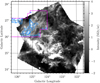Fig. 1

Large-scale view of the Polaris Flare as observed with the Spire instrument of the Herschel observatory at 500 µm. The magenta polygon shows the CO surveyed region, and blue contours show the smoothed integrated CO (J = 2−1) intensity emission at 2.5 and 4 K km s⁻¹.

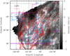Fig. 2

Zoomed-in view toward the striation region. Optical polarization segments (red lines) are overplotted on the dust continuum emission map of the Polaris Flare as observed with Herschel at 500 µm. A line is shown for scale in the top left corner of the figure, corresponding to a degree of polarization of p = 2%. Blue contours correspond to the ¹²CO integrated intensity as in Fig. 1.

3 Starlight polarization data

Optical polarimetric observations were performed by Panopoulou et al. (2015) with the RoboPol polarimeter (King et al. 2014; Ramaprakash et al. 2019), which is mounted at the Skinakas observatory in Crete, Greece¹. RoboPol is a quadruple-beam (four-channel) imaging polarimeter that measures the q and u relative Stokes parameters simultaneously.

This is achieved by splitting the observed light ray into four beams with two Wollaston prisms. For this work, we used stellar measurements in the entire unobstructed field of view (FOV) of RoboPol, as detailed in Panopoulou et al. (2015).

RoboPol is a one-shot Polarimeter that can achieve an accuracy similar to that obtained with conventional dual-beam Polarimeters in significantly less time because it has no moving parts. The main limitation of the design of RoboPol is that a single source is projected into four spots on the same CCD camera. As a result, the point spread functions of nearby stars can sometimes overlap on the CCD (we refer to these sources as blended). We have employed a supervised machine-learning algorithm in order to remove blended measurements.

We applied several selection criteria to remove blended sources or sources affected by other systematics. In the first step, we excluded measurements with an S/N in the degree of polarization lower than 2.5. Low S/N measurements like this introduce statistical biases in the degree of polarization (Vaillancourt 2006; Plaszczynski et al. 2014) and the spread of the polarization angle distribution (Pattle et al. 2017), which is used to estimate the magnetic field strength (Sect. 5.2). Then we removed overlapping stars using a convolutional neural network (CNN). Finally, we used the empirical relation between the degree of polarization and dust extinction, in order to remove outliers from the sample. The last two steps are described in detail in Appendix A.

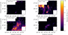Fig. 3

Integrated intensity maps of CO (J = 2−1). The velocity integration interval is shown in the top left corner of each panel. Velocities are in km s⁻¹.

4 CO gas properties

The CO moment maps were constructed using the equation (Miville-Deschênes et al. 2003; Miville-Deschênes & Martin 2007) $I_{m} = \frac{\sum T_{mb} υ^{m} Δ υ}{I_{0}},$ ${I_m} = {{\sum {{T_{{\rm{mb}}}}{\upsilon ^m}{\rm{\Delta }}\upsilon } } \over {{I_0}}},$ (1)

where I₀ is the zeroth-moment map, defined as I₀=∑T_mbΔυ, Δυ = 0.32 km s⁻¹ is the spectral resolution of the CO data, and m = 1, 2 are the indices of the first and second moments, respectively. The zeroth-moment represents (I₀) the total CO intensity measured in Κ km s⁻¹, the first moment (I₁) is the LOS-averaged velocity measured in km s⁻¹, and the square of the second moment ( $\sqrt{I_{2}}$ ${\sqrt {{I_2}} }$ ) corresponds to the velocity dispersion measured in km s⁻¹.

We explore the CO morphological and kinematic properties in this section. Figure 3 shows four different maps of the CO (J = 2−1) intensity integrated over various small velocity ranges, which are indicated in the upper left corner of each panel. Velocities are measured with respect to the local standard of rest (LSR).

Most of the CO gas has negative velocities, consistent with the CO (J = 1 − 0) map of the region shown in Dame et al. (2001), which had a beam size of 0.25 square degrees. Our new CO (J = 2−1) survey reveals the morphology of the gas at a detail comparable to that of Herschel; the FWHM of the SPIRE beam at 500 µm is 36.6″ (Griffin et al. 2010). In the upper left panel of Fig. 3, which corresponds to positive velocities, some sparsely distributed CO structures are visible, but their emission is very weak and may not be associated with the Polaris Flare. We distinguish two negative velocity slices that show maximum CO emission. The upper right panel shows a bright region of CO in the upper left part of the surveyed region, at l, b ~ 126°00′, 27°00′ with an intensity of ~ 10 Κ km s⁻¹. In the bottom left panel, most of the CO is emitted from the lower right portion of the surveyed region toward l, b ~ 125°30′, 26°20′. There is also a CO structure in the bottom right panel that corresponds to velocities from −3.8 to −4.8 km s⁻¹, but its intensity is weaker than in other panels. Most of the CO in the striation region in the Polaris Flare moves with an LOS velocity in the range [0, −3.8] km s⁻¹.

Figure 4 shows the I₀ map of ¹²CO (J = 2−1), which is integrated over the entire velocity range of the spectra. The map is noisy, mainly due to bad weather conditions during the observations and short integration times needed for covering a wide area. We computed the amplitude of the noise (σ_noise) by calculating the intensity rms in velocity channels free of CO emission. We find that σ_noise varies from 0.35 Κ km s⁻¹ up to ~0.87 Κ km s⁻¹ within the surveyed region; high noise is encountered close to the edges of this region. We consider the median σ_noise, which is ~0.45 K km s⁻¹, as the characteristic amplitude of the noise in the CO data.

The observed I₀ map does not show the prominent CO linear structures found in regions with striations within other molecular clouds (e.g., Goldsmith et al. 2008). The observed CO structures have relatively low aspect ratios (blobby more than filamentary; Fig. 4). We observe enhanced CO intensity in regions with the highest dust emission (Fig. 2), but the morphologies of the observed CO and dust intensity structures are not well correlated. Dust structures are thin and aligned with the POS magnetic field, while CO structures are thick and inclined with respect to the POS magnetic field orientation. The dust emission maps in Figs. 1 and 2 correspond to the 500 µm band of the SPIRE instrument on Herschel. The morphology of the dust emission structures in the other two SPIRE bands at 200 and 350 µm shows the same behavior.

In order to minimize the noise in the moment maps, we smoothed the data with a Gaussian kernel of FWHM = 2.5′; this is the minimum kernel size that sufficiently minimizes the noise in the map. After the smoothing, we constructed the three moment maps. Then, we masked out every pixel with an integrated intensity I₀ ≤σ_noise. In the top left panel of Fig. 5, we show the masked and smoothed I₀ map.

In the I₀ map, we observe a prominent quasiperiodic structure. In the top right panel of Fig. 5, we show the CO intensity profile along the white line in the I₀ map (upper left panel in Fig. 5). The CO intensity as a function of distance along this line oscillates quasiperiodically with a characteristic wavelength of ~1 pc, assuming that the Polaris Flare is located at ~340 pc (Panopoulou et al. 2022). In the same panel, we also display the dust emission intensity as a function of position in the three SPIRE bands at 250, 350, and 500 µm, obtained from maps smoothed to the same low resolution as the smoothed I₀ map. The three Herschel bands present almost identical morphological features, except for the normalization of the intensity, which varies due to the modified blackbody nature of the dust emission. In the dust emission profiles, we observe a large-scale fluctuating pattern at ~ 1 pc, similar to that found in the CO emission. However, the first dust intensity local maximum at ~ 1 pc is not colocated with the CO peak. The dust intensity profiles present subparsec fluctuations that are not observed in the CO intensity. The small-scale fluctuations may be the reason why the dust intensity peak at ~1 pc does not exactly match the CO intensity peak. The observed periodic pattern in the CO intensity is 17° off the mean POS magnetic field orientation, which is traced by dust polarization (magenta segments). In contrast to previous observations, where quasiperiodic CO structures tend to be orthogonal to the magnetic field orientation (Goldsmith et al. 2008; Palmeirim et al. 2013; Cox et al. 2016), we observe quasiperiodic structures that tend to be parallel to the mean magnetic field orientation. We discuss noise and resolution effects in Sect. 6.

We inspected the I₁ map for potential evidence of quasiperiodicity similar to the one observed in the I₀ map. However, correlating the I₀ and I₁ maps is challenging because in some cases, the quasiperiodic wave pattern may be imprinted on either the I₀ or in the I₁ map, but never in both maps. We present two thought experiments in order to demonstrate the above statement: a) If we consider that the quasiperiodicity is induced by a propagating plane wave polarized in the POS, then this wave should have no LOS velocity component, hence should be undetectable in the I₁ map. b) If the polarization of the wave is along the LOS, then the wave should not be imprinted on the I₀ map. We can imagine multiple plane waves polarized along the LOS that induce a detectable pattern in the I₁ map, but are undetectable in the I₀ map. Therefore, we refrain from drawing any conclusion from the correlation of the I₀ and I₁ maps.

In the zeroth-moment map, we identify two regions with prominent CO emission. The first region (region I) is shown with the dotted black rectangle in Fig. 5, and the second region (region II) is shown with a solid black polygon. These two regions have different kinematic properties. Region I has LSR velocities close to 0 km s⁻¹, as indicated by the first-moment map (bottom left panel in Fig. 5), and a velocity dispersion close to ~ 1 km s⁻¹, as indicated by the square root of the second-moment map (bottom right panel). Region II has LSR velocities ranging from −4.0 to −1.0 km s⁻¹ (bottom left panel of Fig. 5), and the velocity dispersion is close to 2 km s⁻¹ on average, with a maximum dispersion close to 4 km s⁻¹. In Fig. 6 we show the averaged CO spectra of the two regions.

We detected ¹³CO (J = 2−1) only toward a few LOSs that coincide with peaks in the ¹²CO intensity. Cyan boxes in Fig. 4 correspond to the regions in which we detected the ¹³CO line. In these regions, the ¹³CO lines are ~4σ detections and their maximum intensity is almost an order of magnitude lower than that of ¹²CO (inset panels).

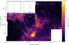Fig. 4

CO integrated intensity moment map at native resolution, without any filtering or masking. Cyan box-shaped regions are defined by the positions at which we detected the ¹³CO (J = 2−1) line. Inset panels show the mean spectra of ¹²CO (magenta) and ¹³CO (blue) within the cyan boxes. The intensity of the ¹³CO emission is approximately an order of magnitude lower than ¹²CO.

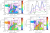Fig. 5

¹²CO (J = 2−1) moment maps smoothed at a resolution of 2.57′. The circular beam in the left corner of each panel shows the Gaussian kernel used for smoothing the data. Magenta segments show the POS magnetic field orientation as traced by optical dust polarization. A scale segment is shown in the upper left corner in each panel. Pixels with a total CO intensity lower than 1.1 (K km s⁻¹) have been masked out. The dotted black rectangle defines the boundaries of region I, and the solid polygon defines region II. The black labels (I, II) are the region identifiers. Top left panel: Intensity (zero-moment) map of CO. Upper right panel: Intensity profiles along the white line shown in the I₀ map. The left vertical axis corresponds to the CO (J = 2−1) integrated intensity. The right vertical axis corresponds to the dust intensity of the three Herschel bands of the SPIRE instrument. The wavelength of each band is shown in the legend. The quasiperiodicity of the CO intensity fluctuations is prominent across this line. The wavelength of the pattern is ~1 pc. Dust intensity profiles are more complex than the CO profile, showing several subparsec features. Bottom left panel: Centroid velocity (I₁, first moment) map of CO. Right panel: Velocity dispersion of CO ( $\sqrt{I_{2}},$ $\sqrt {{I_2}} ,$ square root of the second-moment map).

5 Magnetic field properties

5.1 Magnetic field morphology

We explored the magnetic field morphology of regions I and II. Magenta segments in Fig. 5 correspond to the POS magnetic field orientation, as traced by optical dust polarization data. In region I, the magnetic field orientation is parallel to the Galactic latitude axis on average, while in region II, the magnetic field orientation is offset with respect to the Galactic latitude axis. The difference in the mean magnetic field orientation of the two regions is more prominent in the distribution of polarization angles (Fig. 7); polarization angles are reported in the Galactic reference frame, following the IAU convention. In region I, the mean polarization angle is −2°, and in region II, the mean angle is −16°.

Overall, the two regions have different CO properties (morphological and kinematic) and mean magnetic field orientations. From the 3D extinction map of Green et al. (2018), we found that the two regions are not colocated. Region II is located at ~335 pc, and region II lies at ~340 pc. Both regions could be parts of the Polaris Flare, but the 3D extinction map is noisy there, and we cannot make stronger conclusions. We also explored the 3D map of Leike et al. (2020), but it is also noise-dominated toward this region. We do not observe any sign of interaction between the two regions.

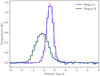Fig. 6

Averaged CO spectra toward regions I and II. The width of each bin is equal to the spectral resolution. Colored lines correspond to Gaussian fits. The mean velocities of regions I and II are −0.80, and −2.22 km s⁻¹, respectively. The FWHM line widths in regions I and II are 1.39 and 2.61 km s⁻¹, respectively.

5.2 Magnetic field strength

We estimated the POS magnetic field strength (B_POS) of each region following the method of Skalidis & Tassis (2021). The POS magnetic field strength can be estimated using $B_{POS} \approx \sqrt{4 π ρ} \frac{σ_{u,turb}}{\sqrt{2 δ θ}},$ ${{\rm{B}}_{{\rm{POS}}}} \approx \sqrt {4\pi \rho } {{{\sigma _{{\rm{u,turb}}}}} \over {\sqrt {2\delta \theta } }},$ (2)

where ρ is the gas density, σ_u,turb is the gas turbulent velocity, and δθ is the dispersion of polarization angles.

The assumption of this method is that gas turbulent kinetic energy is exchanged between kinetic and magnetic forms. Equation (2) has been tested in ideal-MHD simulations without self-gravity and was found to produce accurate estimates of the projected mean magnetic field strength for a wide range of Alfvénic (0.1 ≤ ℳ_A ≤ 2) and sonic (0.5 ≤ ℳ_s ≤ 20) Mach numbers (Skalidis et al. 2021).

5.2.1 Polarization angle intrinsic spread

In the B_POS estimation (Eq. (2)), δθ corresponds to the intrinsic spread induced by gas turbulent motions. Estimating the intrinsic dispersion of polarization angles (δθ₀) from the observed distribution of the polarization angles may be challenging when the S/N ≲ 3. Then the observational uncertainties of the polarization angles are comparable to the observed spread of the polarization angle distribution. Observational uncertainties tend to bias the estimation of δθ₀ toward higher values (Pattle et al. 2017); overestimating δθ₀ leads to underestimating B_POS (Eq. (2)). In regions I and II, the maximum observational uncertainty of the polarization angles is ~16°, and the observed δθ are ~7.7º and ~15°, respectively (Fig. 7). Thus, the observed δθ are likely biased due to the large observational uncertainties. The statistical bias in δθ is usually treated by subtracting the observed spread with the mean observational uncertainty in quadrature (e.g., Panopoulou et al. 2016; Skalidis et al. 2022). Here we employed a Bayesian approach in order to properly mitigate the observational uncertainties and derived the posterior distribution of δθ₀

We fit Gaussians to the polarization angle distributions of both regions because numerical simulations show that this is the intrinsic shape of the polarization angle distributions induced by MHD turbulence (e.g., Heitsch et al. 2001; Falceta-Gonçalves et al. 2008; Skalidis & Tassis 2021). A normalized Gaussian distribution is characterized by two free parameters: 1) the mean angle (θ₀), and 2) the spread, which is the intrinsic spread (δθ₀). We assumed uniform priors with θ₀ ϵ [−90°, 90°], and δθ₀ ϵ [0°, 50°]; spreads larger than 50° are uninformative of the intrinsic (turbulent) spread due to the π ambiguity in polarization angles. We also assumed Gaussian error bars. Each polarization angle data point (θ_i) is characterized by the following data equation: $θ_{i} = 𝒢 (θ_{0}, δ θ_{0}) + 𝒢 (0, σ_{i}),$ ${\theta _i} = {\cal G}\left( {{\theta _0},\delta {\theta _0}} \right) + {\cal G}\left( {0,{\sigma _i}} \right),$ (3)

where 𝒢 denotes a Gaussian probability density function, and σ_i is the observational uncertainty of the polarization angles. A detailed discussion of the Bayesian modelling of the intrinsic spread can be found in Pelgrims et al. (2023).

We maximized the following log-likelihood using the emcee Markov chain sampler (Foreman-Mackey et al. 2013), $\ln ℒ = - \sum_{i = 1}^{N} [\ln \sqrt{2 π} + \ln δ θ_{t o t, i} + \frac{{(θ_{i} - θ_{0})}^{2}}{2 δ θ_{t o t, i}^{2}}],$ $\ln {\cal L} = - \sum\limits_{i = 1}^N {\left[ {\ln \,\,\sqrt {2\pi } + \ln \delta {\theta _{tot,i}} + {{{{\left( {{\theta _i} - {\theta _0}} \right)}^2}} \over {2\delta \theta _{tot,i}^2}}} \right],}$ (4)

where $δ θ_{t o t, i}^{2} = δ θ_{0}^{2} + σ_{i}^{2}$ $\delta \theta _{tot,i}^2 = \delta \theta _0^2 + \sigma _i^2$ , and denotes the observed polarization angle spread. In the distribution of polarization angles of region II, we applied a 4 σ clipping in order to remove measurements that are likely intrinsically polarized stars. The polarization signal of these stars probes the properties of the intrinsic polarization mechanism and not the ISM magnetic field properties. In total, only two measurements were discarded.

The posterior distributions of θ₀ and δθ₀ for both regions are shown in Fig. 8. We computed the mean θ₀ and δθ₀ of the posterior distributions with their corresponding 68% confidence intervals. The 68% percentile for region I is $δ θ_{0} = {2.28}_{- 1.03}^{+ 1.30}$ $\delta {\theta _0} = 2.28_{ - 1.03}^{ + 1.30}$ , and for region II, it is $δ θ_{0} = {8.4}_{- 0.63}^{+ 0.67}$ $\delta {\theta _0} = 8.4_{ - 0.63}^{ + 0.67}$ degrees. These values are significantly different than the intrinsic spread that would be obtained by following the simplistic quadratic subtraction, which assumes uniform observational uncertainties of the polarization angle spread and the mean observational uncertainty (e.g., Panopoulou et al. 2016; Skalidis et al. 2022); with the quadrature subtraction, we obtain for regions I and II that δθ₀ is 1.87° and 12.6°, respectively. In contrast, the Bayesian approach propagates the uncertainty of each measurement to the posterior distribution, and hence resembles the intrinsic spread better.

Region I contains only 46 reliable polarization measurements, and δθ₀ is an upper limit that yields a lower limit for B_POS. The intrinsic spread is statistically consistent with zero, which means that B_POS estimated from Eq. (2) would be infinite. Since the upper limit of B_POS is unconstrained there, we proceed with the magnetic field strength estimation only for region II, where we have 202 trustworthy measurements and δθ₀ is statistically constrained.

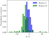Fig. 7

Normalized distributions of polarization angles for both regions. The size of each bin has been optimized using Bayesian analysis from astropy, in order to reflect the intrinsic shape of each distribution.

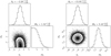Fig. 8

1D, and 2D marginalized posterior distributions of θ₀, and δθ₀ for regions I (left panel) and II (right panel). These plots were produced with the corner plot function of Foreman-Mackey (2016).

5.2.2 Density and turbulent gas velocity estimation

The gas density is $ρ = μ m_{H_{2}} n_{H_{2}}$ $\rho = \mu {m_{{{\rm{H}}_2}}}{n_{{{\rm{H}}_2}}}$ , where µ = 2.8 is the mean molecular weight, considering the helium abundance (Fig. A.1; Kauffmann et al. 2008). Quantities $m_{H_{2}}$ ${m_{{{\rm{H}}_2}}}$ , and $n_{H_{2}}$ ${n_{{{\rm{H}}_2}}}$ denote the mass of the hydrogen molecule and the molecular hydrogen number density, respectively.

In principle, 3D extinction maps might be used (e.g., Green et al. 2018; Lallement et al. 2019; Leike et al. 2020) to estimate the LOS dimension of the Polaris Flare and hence $n_{H_{2}}$ ${n_{{{\rm{H}}_2}}}$ , as has been done for other clouds (Zucker et al. 2021; Tritsis et al. 2022a). However, we found that the 3D extinction maps of Green et al. (2018) and Leike et al. (2020) did not have enough sensitivity toward the striation region to draw any conclusion on the depth of the cloud.

The mean density of the striation region has previously been considered to be $300 \leq n_{H_{2}} \leq 1000 {cm}^{- 3}$ $300 \le {n_{{{\rm{H}}_2}}} \le 1000\,\,{\rm{c}}{{\rm{m}}^{ - 3}}$ (Panopoulou et al. 2016). However, by modeling the ¹²CO, and ¹³CO emission lines, we infer that the maximum gas density can be as high as 1200 cm⁻³ (Appendix B). In order to be conservative, we adopted this value as an upper limit for $n_{H_{2}}$ ${n_{{{\rm{H}}_2}}}$ , and hence we adopted that $300 \leq n_{H_{2}} \leq 1200 {cm}^{- 3}$ $300 \le {n_{{{\rm{H}}_2}}} \le 1200\,{\rm{c}}{{\rm{m}}^{ - 3}}$ .

To estimate the turbulent velocities, we used the line width of the CO emission spectra. The width of the emission lines is broadened due to thermal and turbulent gas motions. In order to estimate the turbulent broadening, we subtracted the thermal broadening in quadrature. The thermal broadening depends on the gas kinetic temperature (T_K), which is unknown. We assumed T_K values based on the literature. Heiles & Troland (2003) studied the properties of H I clouds in our Galaxy using H I absorption data. They found that the mean temperature of atomic gas is ~50 K. Since the Polaris Flare is a diffuse molecular cloud, and in molecular clouds, gas is colder than in atomic clouds, we considered T_K = 50 K to be an upper limit to the kinetic temperature. T_K of molecular gas is ~1.5 times lower than that of atomic gas (Goldsmith 2013), hence we adopted T_K = 35 K as a reference temperature. We considered T_K = 20 K as the lower limit to the kinetic temperature.

The observed spread of the CO (J = 2−1) emission line is 1.13 km s⁻¹. For T_K = 50 K and T_K = 20 K, we estimated by subtracting in quadrature the thermal line spread from the observed one that the turbulent broadening is 1.03 and 1.09 km s⁻¹, respectively. Variations of T_K lead to a 0.06 km s⁻¹ uncertainty in the estimated σ_u,turb. If we consider that T_K = 100 K, which is a typical temperature of molecular gas in photodissociation regions (PDRs), then σ_u,turb ≈ 0.92 km s⁻¹. This means that if we allow T_K to range from 20 to 100 K, the uncertainty on σ_u,turb becomes 0.2 km s⁻¹. However, for the striation region, we favor T_K ≲ 50 K (Appendix B). In order to be conservative, we considered that the uncertainty of σ_u,turb originating from T_K is 0.1 km s⁻¹. Thus, we estimated the turbulent broadening to be σ_u,turb = 1.0 ± 0.1 km s⁻¹. We estimated that B_POS (Eq. (2)) ranges from 38 to 76 µG, while in the same table, we also report the B_POS estimate at intermediate densities, n = 600 cm⁻³, for reference. The Alfvén speed, defined as $V_{A} = B_{POS} / \sqrt{4 π ρ}$ ${V_{\rm{A}}} = {{{B_{{\rm{POS}}}}} \mathord{\left/ {\vphantom {{{B_{{\rm{POS}}}}} {\sqrt {4\pi \rho } }}} \right. \kern-\nulldelimiterspace} {\sqrt {4\pi \rho } }}$ , is $V_{A} = σ_{u,turb} / \sqrt{2 δ θ} = 2.0 \pm 0.1 km s^{- 1}$ ${V_{\rm{A}}} = {{{\sigma _{{\rm{u,turb}}}}} \mathord{\left/ {\vphantom {{{\sigma _{{\rm{u,turb}}}}} {\sqrt {2\delta \theta } }}} \right. \kern-\nulldelimiterspace} {\sqrt {2\delta \theta } }} = 2.0 \pm 0.1\,{\rm{km}}\,{{\rm{s}}^{ - 1}}$ .

Table 1

Region parameters.

5.3 Sonic and Alfvénic Mach numbers

According to the ST method, the projected Alfvénic Mach number is $ℳ_{A}^{1 D} \equiv σ_{turb} / V_{A} \approx \sqrt{2 δ θ}$ ${\cal M}_A^{1{\rm{D}}} \equiv {{{\sigma _{{\rm{turb}}}}} \mathord{\left/ {\vphantom {{{\sigma _{{\rm{turb}}}}} {{{\rm{V}}_{\rm{A}}}\,\, \approx \,\,\sqrt {2\delta \theta } }}} \right. \kern-\nulldelimiterspace} {{{\rm{V}}_{\rm{A}}}\,\, \approx \,\,\sqrt {2\delta \theta } }}$ . We estimated the total ℳ_A of the cloud by multiplying $ℳ_{A}^{1 D}$ ${\cal M}_A^{1{\rm{D}}}$ by $\sqrt{3}$ $\sqrt 3$ , assuming isotropic turbulent properties. For region II, we obtain that ℳ_A ≈ 0.94 ± 0.02, which means that turbulence is sub-Alfvénic, hence the magnetic field is dynamically dominant there. The estimated ℳ_A should be treated as an upper limit because turbulence in the ISM is not isotropic (Higdon 1984; Desai et al. 1994; Backer & Chandran 2000; Shaikh & Zank 2007; Planck Collaboration Int. XXXV 2016), and for anisotropic turbulence, the factor that connects $ℳ_{A}^{1 D}$ ${\cal M}_A^{1{\rm{D}}}$ with the total ℳ_A is lower than $\sqrt{3}$ $\sqrt 3$ (Beattie et al. 2020). However, even for isotropic turbulence, the correction factor that connects the projected with the 3D Mach numbers can be lower than $\sqrt{3}$ $\sqrt 3$ (Stewart & Federrath 2022).

We estimated the sonic Mach number $ℳ_{S}^{1 D} \equiv σ_{turb} / c_{s}$ ${\cal M}_{\rm{S}}^{1{\rm{D}}} \equiv {{{\sigma _{{\rm{turb}}}}} \mathord{\left/ {\vphantom {{{\sigma _{{\rm{turb}}}}} {{{\rm{c}}_{\rm{s}}}}}} \right. \kern-\nulldelimiterspace} {{{\rm{c}}_{\rm{s}}}}}$ , where c_s is the sound speed. For isotropic turbulence, $ℳ_{S} \approx \sqrt{3} ℳ_{S}^{1 D}$ ${{\cal M}_{\rm{S}}} \approx \sqrt 3 {\cal M}_{\rm{S}}^{1{\rm{D}}}$ , which yields that ℳ_s ~ 3.9–6.5 for region II. All the estimated quantities are summarized in Table 1.

6 CO chemistry in striations and the role of magnetic fields

Magnetic fields affect the dynamical properties of clouds in the ISM and hence their chemical evolution. Strongly dynamical magnetic fields tend to suppress molecule formation (Walch et al. 2015; Seifried & Walch 2016; Pardi et al. 2017; Girichidis et al. 2018). Magnetic fields are not easily compressed perpendicular to the field lines because of magnetic tension and pressure. Simulated magnetized clouds are more diffuse than their corresponding nonmagnetized counterparts. As a result, gas in magnetized clouds is poorly shielded, hence magnetized clouds tend to have higher CO-dark H₂ abundance than nonmagnetized clouds, which are richer in CO (Seifried et al. 2021).

Molecule formation is also affected by the relative alignment between the magnetic field and the cloud structure, or the velocity flow. For example, in the simulations of Seifried & Walch (2016), when the magnetic field is aligned with the main filament axis, the abundances of C, C⁺, and CO change abruptly from the outer parts to the center of the filament. When the magnetic field is perpendicular to the filament axis, the carbon-based species abundances have shallower gradients toward the center of the filament. Furthermore, amplified magnetic fields from colliding flows form a critical angle with the upstream velocity, which determines whether molecule formation is suppressed or enhanced (Iwasaki et al. 2019; Iwasaki & Tomida 2022). Overall, all the aforementioned numerical studies suggest that the ISM magnetic field affects the formation of molecular gas mainly by setting a preferred orientation along which gas accumulation, and hence molecule formation, can take place. Observationally, there is evidence supporting this theoretical scenario (Skalidis et al. 2022).

In the current study, we explore the role of magnetic fields in the molecule formation in striations. Compressions in our target region are most likely formed by propagating MHD waves (Tritsis & Tassis 2016), as indicated by the prominent periodic structure in the CO intensity map (Fig. 5), and not by colliding flows, as is the case of the aforementioned numerical simulations. Therefore, we cannot directly compare our observations and the simulated colliding flow models. However, V_A seems to be an important parameter for initiating the suprathermal chemistry (Federman et al. 1996; Visser et al. 2009). Below, we explore the conditions under which wave modes could contribute to the CO formation within the striation region in the Polaris Flare.

6.1 Compressible MHD modes as agents of CO formation

Striations are considered to form due to the propagation of compressible MHD modes (Tritsis & Tassis 2016). Strong observational evidence supporting this theory comes from the quasiperiodic patterns observed in CO and dust intensity maps (Goldsmith et al. 2008; Palmeirim et al. 2013; Malinen et al. 2014; Cox et al. 2016). In the Polaris Flare, we find a prominent quasiperiodic pattern in the CO zeroth-moment and dust intensity maps, with a periodicity that is almost parallel to the mean magnetic field orientation (Fig. 5) and not perpendicular, as has been previously observed (Goldsmith et al. 2008). However, we note that the dust emission map is periodic both along and across the mean magnetic field orientation.

The contrast in the CO zeroth-moment map (~43%) is higher than the contrast of the $N_{H_{2}}$ ${{\rm{N}}_{{{\rm{H}}_2}}}$ map (18%). Differences in the column density contrast between gas and CO maps have also been observed in numerical simulations (Tritsis & Tassis 2016). The difference in the contrast of the two maps indicates that it is unlikely that CO could have preexisted and been compressed by a propagating MHD wave. It is more probable that the CO formation has been enhanced by a propagating MHD wave. First, we examine the case of waves in compressible gas, and then the incompressible case.

Compressible linear MHD perturbations can propagate in the form of fast and slow magnetosonic modes. When V_A ≫ c_s, the characteristic propagation speed for the fast and slow modes is V_A, and c_s, respectively. Fast modes propagate isotropically, while slow modes, which oscillate as sound waves when V_A ≫ c_s, cannot propagate perpendicular to the magnetic field lines. Thus, both slow and fast modes could form the quasiperiodic pattern in the observed CO zeroth-moment map (Fig. 5) because the propagation axis of this pattern is slightly different from the mean magnetic field orientation.

The characteristic timescale of CO formation (τ_CO) in general differs from the MHD wave periods (τ_waves). If τ_CO > τ_waves, then MHD waves compress and rarefy the gas before CO has enough time to form. If τ_CO < τ_waves, then CO can form at an enhanced rate within the compressed regions produced by the passage of the MHD wave. The slow and fast modes have different characteristic timescales for the same wavelengths. Using the wavelength (~ 1 pc) of the observed quasiperiodic pattern in the CO intensity map, we obtain that the period of a fast mode should be τ_fast ≈ 0.48 Myr, while for a slow mode, the period should be τ_slow = 2.1–3.4 Myr. The estimated range of τ_slow corresponds to the assumed T_K range (20–50 K). For the Polaris Flare, we estimate that τ_CO = 0.03–1.0 Myr (Appendix C). If τ_CO = 1.0 Myr, then τ_fast < τ_CO < τ_slow. In this case, fast modes oscillate much faster than the typical CO formation timescale, hence are unlikely to have contributed to the CO formation. If τ_CO = 0.03 Myr, then τ_CO < τ_fast < τ_slow, hence both fast and slow modes could be responsible for the CO enhancement. We note that slow modes are slower than the CO formation timescale for both τ_CO limits.

In the Polaris Flare, the dust intensity maps follow a power-law behavior with spectral index −2.65 (Miville-Deschênes et al. 2010). The inertial range of the power spectrum extends down to 0.01 pc, implying that MHD wave-modes with such short wavelengths could be observed. However, there is a minimum wavelength (λ_f,min) above which fast modes could be observable in the CO (J = 2−1) intensity map. The minimum wavelength corresponds to fast modes oscillating with periods τ_fast ≥ τ_CO, where τ_fast = λ/ V_A. The condition τ_fast ≥ τ_CO is satisfied when λ ≥ λ_f,min, where λ_f,min = τ_co × V_a ≈ 2 pc for τ_CO = 1 Myr, and λ_f,min = 0.06 pc for τ_CO = 0.03 Myr.

For the slow modes, we estimate that the minimum wavelength is λ_s,min = τ_CO × c_s ≈ 0.28–0.44 pc, when τ_CO = 1 Myr, where the uncertainty on λ_s,min comes from the T_K uncertainty (Sect. 5.2.1). Similarly, we estimate that the minimum wavelength for τ_CO = 0.03 Myr is λ_s,min = τ_CO × c_s ≈ 0.008–0.013 pc. Overall, slow modes are characterized by lower minimum wavelengths than fast modes due to their lower propagation speeds.

The CO intensity profile in Fig. 5 does not show evidence of wave modes with wavelengths shorter than 1 pc. However, this could be related to sensitivity issues because subparsec wavelength modes might induce intensity contrast below the sensitivity limit of our observations. Thus, we cannot exclude the possibility of subparsec-wavelength modes enhancing the formation of CO, but the dominant detected wavelength is ~1 pc. The subparsec wave features in the dust emission profiles (upper right panel in Fig. 5) are close to the spatial resolution limit, hence might be artifacts of the smoothing.

6.2 Role of Alfvén waves in the formation of CO

Ambipolar diffusion decouples ions and neutrals, hence perturbations with timescales longer than the characteristic timescale of ambipolar diffusion do not propagate to neutral gas because they are damped. There are two types of ambipolar diffusion: 1) magnetically driven, and 2) gravitationally driven ambipolar diffusion (Mouschovias et al. 2011). Gravitationally driven ambipolar diffusion requires the existence of a local center of gravity (e.g., a central core that preferentially drags neutral particles past the ions increasing the ratio of mass to magnetic flux of cores relative to their surroundings; Mouschovias et al. 2006; Tassis et al. 2014). Magnetically driven ambipolar diffusion operates at shorter timescales than the gravitationally driven diffusion, which is usually slow since it operates at timescales equal to ~10 Myr (Tassis & Mouschovias 2004). For this reason, we focused only on magnetically driven ambipolar diffusion.

Federman et al. (1996) invoked the magnetically driven ampibolar diffusion to explain the enhancement of ionic products, such as CH⁺, compared to neutral OH. Due to the relative drift between ions and neutrals, Alfvén waves add more energy to C⁺ reactions than to oxygen-based reactions. Thus, the reaction C⁺ + H₂ → CH⁺ + H produces more CH⁺ than the OH produced by the reaction O + H₂ → OH + H. This explains the observed overproduction of CH⁺ without producing much OH. The enhanced CH⁺ abundance increases the formation rate of CO. Alfvén waves propagate along the magnetic field lines with a speed equal to V_A, which implies that Alfvén waves could locally enhance CH⁺, and hence CO, when their velocity is maximum; when the velocity is minimum, CO formation should be negligible. Thus, Alfvén waves could induce the observed quasiperiodic feature in the CO zeroth-moment map (Fig. 5). However, we exclude Alfvén waves because the observed quasi-periodic CO profile is correlated with dust intensity (Fig. 5); Alfvén waves are incompressible and cannot induce temperature (or equally, density) fluctuations.

6.3 Uncertainties in the estimated wave periods

6.3.1 Uncertainties on τ_fast

The wave periods of fast and slow magnetosonic modes depend on their propagation speed. The uncertainties of the propagation speeds, V_A for fast modes and c_s for slow modes, propagate to the estimated wave periods, τ_fast and τ_slow. V_A was constrained with high accuracy based on the dispersion of polarization angles with the method of Skalidis & Tassis (2021). The main uncertainty of V_A comes from the assumptions of the aforementioned method. The method of Skalidis & Tassis (2021) has been tested against a wide range of numerical simulations, and its accuracy was found to be better than a factor of two (Skalidis et al. 2021).

Alternative methods for estimating V_A (DCF; Davis 1951; Chandrasekhar & Fermi 1953) tend to produce higher values than the method of Skalidis & Tassis (2021). According to DCF, the Alfvén speed is V_A = f σ_u,turb/δθ, where f is a fudge factor that is usually considered to be 0.5 (Ostriker et al. 2001; Heitsch et al. 2001; Padoan et al. 2001). With the DCF method, we estimate that V_A = 3.7 km s⁻¹, which yields a period for the fast mode equal to 0.26 Myr. Thus, both the Skalidis & Tassis (2021) and the DCF method suggest that τ_fast > τ_CO when τ_CO = 1 Myr. On the other hand, when τ_CO = 0.03 Myr, we find that τ_CO is always shorter than τ_fast, which means that in this case, fast modes could have contributed to the CO enhancement. Since we do not have precise estimates on τ_CO, we cannot assess whether fast modes play a role in the enhancement of the CO abundance.

6.3.2 Uncertainties on τ_slow

Observationally, it is challenging to constrain T_K and thus c_s. τ_slow scales with T_K as τ_slow $\propto 1 / \sqrt{T_{K}}$ $\propto \,\,{1 \mathord{\left/ {\vphantom {1 {\sqrt {{T_{\rm{K}}}} }}} \right. \kern-\nulldelimiterspace} {\sqrt {{T_{\rm{K}}}} }}$ due to the square root dependence of c_s on T_K. Even if we consider a T_K as high as 100 K, we obtain that c_s < 1 km s⁻¹, which yields that τ_CO < τ_slow, hence slow modes are slower than the CO characteristic timescale. In order to make τ_CO > τ_slow, which implies that slow modes could not enhance the CO formation, we need to increase T_K to a few hundred K, which is unreasonably high for our target region (Appendix B). Therefore, we confidently estimate that τ_CO < τ_slow, which means that slow modes could have enhanced the formation of CO.

6.4 Alternative scenarios

Chen et al. (2017) proposed an alternative formation scenario for striations based on colliding flows. Colliding flows form a dense post-shock sheet-like layer. Within the post-shock layer, secondary oblique shocks develop. Secondary flows form a dense, stagnated sublayer within the primary layer. If the velocity flows within the sublayer vary perpendicular to the post-shock magnetic field, then the sublayer rolls around its primary axis, which tends to be parallel to the mean magnetic field orientation. When the sublayer is viewed perpendicular to the magnetic field lines, the column density map exhibits properties similar to striations: (1) there are structures aligned with the magnetic field, and (2) the periodicity of these structures is perpendicular to the magnetic field orientation. According to the model of Chen et al. (2017), striations are not actual density enhancements but column density effects that are imprinted on the column density maps due to the different path lengths of the corrugated post-shock sublayers.

In the Polaris Flare, turbulence is compressible because ℳ_s > 1. Thus, shocks should develop within the cloud. However, the quasiperiodicity of CO studied here is parallel to the magnetic field, which is distinct from the previously studied linear structures with axes parallel to the magnetic field, but periodic spacing perpendicular to the magnetic field (e.g., Goldsmith et al. 2008). Chen et al. (2017) focused on the formation of structures showing quasiperiodicity perpendicular to the magnetic field, and hence we are not aware whether their model can explain the quasiperiodic pattern studied here. However, the observed periodicity in the CO intensity map is unlikely to be a column density effect. The reason is that we have detected ¹³CO toward the ¹²CO intensity peaks, and we inferred that the density should be highest there compared to the rest of the region (Appendix B). As a result, the observed CO intensity enhancements correspond to actual density increases and not to density corrugations, as proposed by Chen et al. (2017).

An alternative scenario could be that the CO intensity variations correspond to temperature fluctuations. Consider a polytropic equation of state (EoS) for the gas, T ∝ ρ^Γ (Federrath & Banerjee 2015). When Γ = 1, the gas is isothermal; when Γ < 1, small-scale fragmentation takes place, while when Γ > 1, density fluctuations are smoothed out. According to the EoS, temperature and density are two sides of the same coin. In the Polaris Flare, along with the CO intensity quasiperiodic fluctuations, we observe periodic fluctuations of the dust intensity in the three SPIRE bands (Fig. 5). If the dust intensity fluctuations were due to temperature fluctuations, then due to the polytropic EoS, the temperature changes would induce density fluctuations as well. However, the opposite is not always true because the medium can be isothermal (Γ = 1). Overall, periodic temperature fluctuations will always be accompanied by density fluctuations, and hence the observed quasiperiodicity in the CO intensity map cannot be solely due to temperature fluctuations.

7 Conclusions

We have targeted the Polaris Flare region, which is a diffuse molecular cloud with prominent striations. We used the stellar polarization data from Panopoulou et al. (2015) in order to study the magnetic field properties of the striations in the Polaris Flare. We conducted a CO (J = 2−1) survey toward the striation region in order to probe the molecular gas properties and identified two regions (regions I and II) with distinct kinematics properties. The CO intensity enhancements are observed where dust intensity is maximum. However, dust and CO intensity structures are not perfectly correlated.

We used the dispersion of polariation angles in order to estimate the POS magnetic field strength of the two regions with the method of Skalidis & Tassis (2021). We developed a Bayesian approach (Sect. 5.2.1) in order to retrieve the intrinsic dispersion of the polarization angle distributions. For region II, we estimate that turbulence is sub-Alfvénic with an Alfvénic Mach number ℳ_A ≈ 0.94 ± 0.04, an Alfvénic speed V_A ≈ 2.0 ± 0.1 km s⁻¹, and a POS magnetic field strength B_POS = 38–76 µG. The sonic Mach number of the region is estimated to be ℳ_s = 3.9–6.5. All the estimated parameters are summarized in Table 1.

In the CO integrated intensity map, we observe a quasiperiodic structure that is almost perpendicular to the mean magnetic field orientation. The periodicity axis is 17° different from the POS magnetic field orientation, and its wavelength is 1 pc. This is in striking contrast to previous observations of striations, in which CO quasiperiodic structures are aligned with the magnetic field and the periodicity axis is perpendicular to it (e.g., Goldsmith et al. 2008). This quasiperiodic pattern is most likely the imprint of a traveling and compressible MHD wave. The contrast in the CO intensity maps is higher than the contrast in the $N_{H_{2}}$ ${{\rm{N}}_{{{\rm{H}}_2}}}$ map, which indicates that the CO abundance is enhanced. We compared the characteristic timescales of CO formation with the estimated dynamical timescales of MHD waves. Alfvén waves can enhance the CO abundance via diffusion processes (Federman et al. 1996), but this is unlikely for the Polaris Flare, where the observed quasi-periodic CO intensity is correlated with dust intensity (Fig. 5). We find that a slow mode with a velocity 0.3–0.45 km s⁻¹ and period 2.1–3.4 Myr could have enhanced the CO abundance. However, given the τ_CO uncertainties, the fast magnetosonic modes could also have played some role in the CO enhancement of the target region.

Acknowledgements

We thank the referee, Daniel Seifried, for very constructive comments which improved the manuscript. We thank J. Bieging for advice on the CO data reduction. We gratefully acknowledge the large observing time commitment provided by the Arizona Radio Observatory, and the help of the staff in conducting observations. This work was supported by NSF grant AST-2109127. A.T. acknowledges support by the Ambizione grant no. PZ00P2_202199 of the Swiss National Science Foundation (SNSF). This project has received funding from the European Research Council (ERC) under the European Unions Horizon 2020 research and innovation programme under grant agreement no. 771282. K.T. acknowledges support from the Foundation of Research and Technology – Hellas Synergy Grants Program through project POLAR, jointly implemented by the Institute of Astrophysics and the Institute of Computer Science. G.V.P. acknowledges support by NASA through the NASA Hubble Fellowship grant #HST-HF2-51444.001-A awarded by the Space Telescope Science Institute, which is operated by the Association of Universities for Research in Astronomy, Incorporated, under NASA contract NAS5-26555. This research was carried out in part at the Jet Propulsion Laboratory, which is operated by the California Institute of Technology under a contract with the National Aeronautics and Space Administration (80NM0018D0004). This research has made use of data from the Herschel Gould Belt survey (HGBS) project (http://gouldbelt-herschel.cea.fr). The HGBS is a Herschel Key Programme jointly carried out by SPIRE Specialist Astronomy Group 3 (SAG 3), scientists of several institutes in the PACS Consortium (CEA Saclay, INAF-IFSI Rome and INAF-Arcetri, KU Leuven, MPIA Heidelberg), and scientists of the Herschel Science Center (HSC).

Appendix A Identifying blended stars with convolutional neural networks

In order to eliminate blended objects in the Robopol images, we employed the CNN strategy developed by Paranjpye et al. (2020). The CNN model consists of three convolution and max-pooling layers. For the CNN training, we used data from the archive of RoboPol (Blinov et al. 2021).

We trained the CNN in order to identify blended spots. We flagged spots of different stars as “blends” or “normal” by visually inspecting the photometry curve of each spot. Photometry curves show the total photon flux versus the aperture size within which the photometry is performed (Fig. 9 in Panopoulou et al. 2015). When a star behaves normally, the total intensity of a spot converges to a constant value at large radii, while photometry curves of blended stars do not converge at large radii. The reason is that at large radii, adjacent sources contaminate the flux of the target source, and hence the photon intensity grows nonlin-early.

In total, our training sample consisted of 896 blended and 896 normal stars. In order to increase the size of the training sample, we flipped every image vertically. The flipped image is not identical to the unflipped image, but the flagged class (blend or normal) remains the same. In Fig. A.1 we show examples of blended spots used for the training of the CNN. The classified spot is located at the center of each image.

We used ten images that were not included in the training sample from both classes (normal, and blends) in order to test the accuracy of the trained CNN models. We trained the CNN model with a fixed training sample several times, and found that the accuracy of the model fluctuated statistically. In order to eliminate these statistical fluctuations, we trained three different CNN models. These models were chosen due to their low false-positive and false-negative rates. The confusion matrix of the models is shown in Fig. A.2. We applied each model to the polarization data and obtained three different samples of normal stars; one sample from every CNN. Then, these normal-star samples that we obtained from the CNN models were merged into a final sample; normal stars that appeared in several samples were considered only once in the final sample.

After applying the three CNN models, we were still able to identify some outliers in the sample. Outliers can be easily identified because their polarization angle orientations are significantly different than the local averaged polarization orientations, and they also tend to have larger polarization fractions than the local averaged value (e.g., Panopoulou et al. 2015).

In order to remove outliers, we employed the relation between the maximum degree of polarization (p_max) and dust extinction, E(B-V), as was done in Panopoulou et al. (2015). The p_max versus E(B-V) relation is empirical and indicates that at a given E(B-V), ISM-induced dust polarization has an upper limit in p. The upper limit has been widely studied in past years (Andersson & Potter 2007; Frisch et al. 2015; Panopoulou et al. 2015; Skalidis et al. 2018; Planck Collaboration XII. 2020). The most recent updated relation is p(%) ≤ 13 × E(B – V) (Panopoulou et al. 2019); measurements with S/N ≤ 3 were debiased following Vaillancourt (2006). All the measurements that exceeded the p versus E(B-V) limit are likely to be intrinsically polarized sources or blended measurements that were not identified by the CNN. They were hence excluded from the analysis. We computed the extinction of each star from the 3D map of Green et al. (2018). We extracted the distance of each star from the geometric distances from the catalog of Bailer-Jones et al. (2021), which includes measurements from Gaia DR3 (Gaia Collaboration et al. 2021). After we applied the p−E(B-V) filtering, the remaining sample consisted of 631 measurements. Finally, we included all the normal stars from the sample of Panopoulou et al. (2015) that were excluded by our CNN models as true positives. The final sample consists of 711 reliable polarization measurements, which is larger than the original sample of Panopoulou et al. (2015), which consisted of 609 measurements. All stars are located behind the cloud, hence their polarization signal probes the dust and magnetic field properties of the Polaris flare.

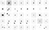Fig. A.1

Images showing blended objects used for the training of the CNN. The size of each image is 64 × 64 pixel.

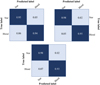Fig. A.2

Normalized confusion matrices of the three neural networks trained for the identification of blended stars in polarization images. The probability of true positives and false negatives is higher than 0.9 for every model. The probability of true negatives and false positives is lower than 0.1 for every model.

In Fig. 2 we show the starlight polarization data (red segments) overplotted on the Herschel emission map. The length of each segment is proportional to the debiased p. A scale segment is shown in the upper left corner of the figure.

Appendix B Ratio of ¹²CO and ¹³CO

The relative abundance ratio of ¹²CO, and ¹³CO can be used to constrain the cloud density and temperature (Pety et al. 2011).

The ¹³CO (J = 2−1) emission is largely undetected toward the striation region. However, the few detections that we have allow us to constrain the local gas conditions.

We focused on LOSs where we detected both the ¹²CO (J = 2−1), and the ¹³CO (J = 2−1) emission lines. We fit the two CO emission lines simultaneously with RADEX (van der Tak et al. 2007). RADEX is a publicly available code that solves the nonlocal thermodynamic equilibrium radiative transfer equations. RADEX takes four free parameters as input: 1) T_K, 2) total CO column density (N_CO), 3) $n_{H_{2}}$ ${n_{{{\rm{H}}_2}}}$ , and 4) CO line width. Only the last is directly observable.

To estimate N_CO, we employed the correlation between $N_{H_{2}}$ ${{\rm{N}}_{{{\rm{H}}_2}}}$ and N_CO, defined as $X_{CO} = N_{CO} / N_{H_{2}}$ ${{{X_{{\rm{CO}}}}{\rm{ = }}{N_{{\rm{CO}}}}} \mathord{\left/ {\vphantom {{{X_{{\rm{CO}}}}{\rm{ = }}{N_{{\rm{CO}}}}} {{{\rm{N}}_{{{\rm{H}}_2}}}}}} \right. \kern-\nulldelimiterspace} {{{\rm{N}}_{{{\rm{H}}_2}}}}}$ . At high densities, all the available carbon is locked in CO molecules and X_CO = 1.6 × 10⁻⁴. This high X_CO corresponds to column densities higher than log N_H > 21 cm⁻², however (Gong et al. 2018). At column densities 20 < log N_H < 21, where the H I → H₂ transition takes place, X_CO is nonlinear (Pineda et al. 2010). The variability of X_CO can be attributed to the different formation timescales of CO and H₂ (Seifried et al. 2017); the CO timescales are shorter than those of H₂.

Direct constraints on X_CO can be obtained only with UV-absorption data (Burgh et al. 2007). We collected archival N_CO and $N_{H_{2}}$ ${{\rm{N}}_{{{\rm{H}}_2}}}$ data (Burgh et al. 2007; Sheffer et al. 2008; Guden-navar et al. 2012), and fit a third-degree polynomial using the Bayesian method described in Sect. 5.2.1, assuming uniform priors (Fig. B.1). We added an additional term in the likelihood (Eq. (4)) that penalized the observational uncertainties of $N_{H_{2}}$ ${{\rm{N}}_{{{\rm{H}}_2}}}$ . There are no observations for log $N_{H_{2}} \geq 21.1$ ${{\rm{N}}_{{{\rm{H}}_2}}} \ge 21.1$ , but this is not a great problem because in the striations of the Polaris Flare log $N_{H_{2}} < 21$ ${{\rm{N}}_{{{\rm{H}}_2}}} < 21$ . The X_CO fit relation is $\log N_{CO} = - 0.18 {(\log N_{H_{2}})}^{3} + 12.43 {(\log N_{H_{2}})}^{2} - 279 \log N_{H_{2}} + 2078.$ $\log \,{{\rm{N}}_{{\rm{CO}}}} = - 0.18\,{\left( {\log \,{{\rm{N}}_{{{\rm{H}}_2}}}} \right)^3} + 12.43\,{\left( {\log \,{{\rm{N}}_{{{\rm{H}}_2}}}} \right)^2} - 279\,\log \,{{\rm{N}}_{{{\rm{H}}_2}}} + 2078.$ (B.1)

Using the $N_{H_{2}}$ ${{\rm{N}}_{{{\rm{H}}_2}}}$ map of the Polaris Flare (André et al. 2010), we find for region I that the median log $N_{H_{2}} = 20.83 {cm}^{- 2}$ ${{\rm{N}}_{{{\rm{H}}_2}}} = 20.83\,{\rm{c}}{{\rm{m}}^{ - 2}}$ , which due to Eq. (B.1) yields that log N_CO ≈ 15.44 cm⁻². The scatter of the points in Fig. B.1 is significant, and hence we consider this value as an order-of-magnitude estimate.

The scatter of N_CO in Fig. B.1 reflects intrinsic variations of the X_CO relation and is not due to observational uncertainties. The correlation between N_CO and $N_{H_{2}}$ ${{\rm{N}}_{{{\rm{H}}_2}}}$ might mainly be affected by three physical quantities (Bisbas et al. 2021): 1) cosmic-ray ionization, 2) far-UV intensity, and 2) metallicity. High cosmic-ray ionization would increase the C⁺ abundance (Goldsmith et al. 2018), which means that not all of the gasphase carbon would be in the form of CO molecules. Thus, for a given column density, C⁺ might be associated with H₂, but not with CO; this gas component is referred to as CO-dark H₂ (van Dishoeck & Black 1988; Sternberg & Dalgarno 1995; Grenier et al. 2005; Langer et al. 2010; Paradis et al. 2012; Pineda et al. 2013). High far-UV intensities photodissociate CO and lead to lower CO abundances. Finally, metallicity is linearly correlated with visual extinction, hence with $N_{H_{2}}$ ${{\rm{N}}_{{{\rm{H}}_2}}}$ . Shielding is proportional to metallicity. Thus, CO is destroyed more efficiently in lower-metallicity environments (Bialy & Sternberg 2016). Metallicity and far-UV intensity variations could affect the column density threshold at which the H I → H₂ transition takes place (Bialy & Sternberg 2016; Gong et al. 2020). The points in Fig. B.1 correspond to sparsely distributed LOSs across our Galaxy, hence each point is sensitive to the local ISM conditions.

For the RADEX input, we assumed some typical values for T_K and $n_{H_{2}}$ ${n_{{{\rm{H}}_2}}}$ : T_K = 20, 50, 100 K, and $n_{H_{2}} = 400, 700, 1000 {cm}^{- 3}$ ${n_{{{\rm{H}}_2}}} = 400,\,700,\,1000\,{\rm{c}}{{\rm{m}}^{ - 3}}$ . The properties of the Polaris Flare should be represented by some pair of $n_{H_{2}}$ ${n_{{{\rm{H}}_2}}}$ , T_K; in total, there are nine pairs. For each pair of $n_{H_{2}}$ ${n_{{{\rm{H}}_2}}}$ , T_K, we determined the column density of the emitted species (¹²CO and ¹³CO) that reproduces the observed values, and hence we obtained a pair of ¹²CO, and ¹³CO column densities (N[¹²CO], N[¹³CO]). Then, we calculated the ratio N[¹²CO]/N[¹³CO]. For every considered pair of $(n_{H_{2}}, T_{K})$ $\left( {{n_{{{\rm{H}}_2}}},\,{{\rm{T}}_{\rm{K}}}} \right)$ , we find that N[¹²CO]/N[¹³CO] ≤ 10. This ratio is significantly lower than the observed ¹²C/¹³C ratio, which in our Galaxy ranges from 30 up to 70 (Langer & Penzias 1990).

The reduced relative abundance of the CO isotopes strongly suggests that isotopic fractionation of CO is taking place (Watson et al. 1976). The isotopic fractionation occurs due to the exothermal ion-neutral reaction $^{13} C^{+} +^{12} CO \to^{12} C^{+} +^{13} CO + ΔE,$ $^{13}{{\rm{C}}^ + }{ + ^{12}}{\rm{CO}}{ \to ^{12}}{{\rm{C}}^ + }{ + ^{13}}{\rm{CO}}\,{\rm{ + }}\,{\rm{\Delta E,}}$ (B.2)

where ∆E/k_B = 35 K. The column density range in which isotopic fractionation is efficient is log N_CO(cm⁻²) = 15–16 (Szűcs et al. 2014), which is consistent with our order-of-magnitude estimate of N_CO, based on Eq. (B.1). The above chemical reaction enhances the abundance of ¹³CO relative to ¹²CO. The carbon monoxide isotopic ratio depends on T_K as (Watson et al. 1976) $\frac{^{12} CO}{^{13} CO} = \frac{^{12} C}{^{13} C} \times e^{- 35 / T_{K}} .$ ${{^{12}{\rm{CO}}} \over {^{13}{\rm{CO}}}} = {{^{12}{\rm{C}}} \over {^{13}{\rm{C}}}} \times {{\rm{e}}^{{{ - 35} \mathord{\left/ {\vphantom {{ - 35} {{{\rm{T}}_{\rm{K}}}}}} \right. \kern-\nulldelimiterspace} {{{\rm{T}}_{\rm{K}}}}}}}.$ (B.3)

It is evident that the isotopic fractionation is effective at low temperatures. When T_K > 100 K, the CO isotopic ratio converges to the ¹³C/¹²C ratio, which is close to 60 in our solar neighborhood (Langer & Penzias 1990). As T_K decreases (T_K ≤ 50 K), then ¹³CO/ ¹²CO increases exponentially (Eq. (B.3)), compared to the elemental carbon ratio.

For a given T_K, we analytically computed the expected CO isotopic ratio (Eq. (B.3)) and compared this value with the RADEX-output N[¹²CO]/N[¹³CO] ratio. When the analytical and RADEX results agreed, we considered that the input T_K represents the actual cloud temperature.

The isotopic ratio of ¹²C/¹³C depends linearly on the Galactocentric distance (D_GC, Milam et al. 2005). For the Polaris Flare, we estimate that D_GC = 8.3 kpc, assuming for the Sun that D_GC = 8.1 kpc (Bobylev & Bajkova 2021). Based on Eq. (3) of Milam et al. (2005), we estimate that ¹²C/¹³C = 63. Without isotopic fractionation, or equally at high temperatures (T_K = 100 K), ¹²CO/¹³CO should be close to 63. The analytic CO isotopic ratio (Eq. (B.3)) is consistent with the ratio obtained from the RADEX-output column densities only when T_K ≈ 20 K. The $n_{H_{2}} = 400 {cm}^{- 3}$ ${n_{{{\rm{H}}_2}}} = 400\,{\rm{c}}{{\rm{m}}^{ - 3}}$ case seems to be unlikely because when we fit the observed emission lines with this density, the data are reproduced only when N(¹²CO) = 3 ×10¹⁶ cm⁻². This value is higher than the N_CO values with log $N_{H_{2}} ({cm}^{- 2}) < 21$ ${{\rm{N}}_{{{\rm{H}}_2}}}\left( {{\rm{c}}{{\rm{m}}^{ - 2}}} \right) < 21$ (Fig. B.1). If we consider a maximum log N_CO(cm⁻²) = 16 (Fig. B.1), then we find that the minimum density that can fit the data is 600 cm⁻³. Overall, regions with detectable ¹³CO should have T_K ≈ 20 K and $n_{H_{2}} \geq 600 {cm}^{- 3}$ ${n_{{{\rm{H}}_2}}} \ge 600\,{\rm{c}}{{\rm{m}}^{ - 3}}$ .

For a deeper understanding of the cloud properties, we modeled the conditions toward the regions in which ¹³CO was detected. We employed the Meudon PDR code (Le Petit et al. 2006). We did not aim to model the average properties of the striation region, but only the specific lines of sight. We used a constant visual extinction A_υ = 1 and explored the kinetic temperature as a function of density and of the UV background intensity (G) relative to the standard Habing interstellar radiation field intensity (ISRF). The cloud was modeled as a two-sided slab with an equal UV field incident on both sides. In the upper panel of Fig. B.2, we show the results of the modeling. T_K is strongly affected by G and weakly affected by $n_{H_{2}}$ ${n_{{{\rm{H}}_2}}}$ ; $n_{H_{2}}$ ${n_{{{\rm{H}}_2}}}$ is important only for the relative CO abundance (lower panel in Fig. B.2). So far, we have inferred that T_K should be close to 20 K. From the PDR modeling, we find that T_K = 20 Κ is achieved only for $n_{H_{2}} = 1200 {cm}^{- 3}$ ${n_{{{\rm{H}}_2}}} = 1200\,{\rm{c}}{{\rm{m}}^{ - 3}}$ , and G = 0.5 This is an upper limit for the density of the striation region. When we assume that the mean UV intensity in the striation region is G ≤ 1, then the average kinetic temperature should be T_K < 50 K, which is consistent with the T_K that we assumed in Sect. 5.2.2.

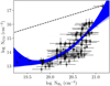Fig. B.1

CO vs. H₂ column density. Black points correspond to archival data. The solid blue lines are 7000 realizations extracted from the posterior distributions of the Bayesian fitting. The dotted black line corresponds to 10⁻⁴ $N_{H_{2}}$ ${{\rm{N}}_{{{\rm{H}}_2}}}$ , which corresponds to clouds in which essentially all carbon is in the form of CO.

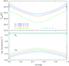Fig. B.2

Results of the PDR modeling for A_v = 1. Upper panel: Kinetic temperature vs. A_v for different gas densities and UV intensities (G). Lower panel: Densities of H₂ and CO vs. A_v.

Appendix C CO formation timescale

We explored the time evolution of CO under dynamical steady state. We used a modified version of the FLASH astrophysical code (Fryxell et al. 2000; Dubey et al. 2008), which includes a chemical network consisting of 115 chemical species and 1600 chemical reactions. Our chemical network was first used in Tritsis et al. (2022b), and the details of the chemical processes and the initial elemental abundances have been presented in Tritsis et al. (2016). We considered a cylindrical cloud geometry and explored two possibilities regarding the physical conditions of the Polaris cloud, based on our estimated densities. In the first case, the H₂ number density was set to $n_{H_{2}} = 800 {cm}^{- 3}$ ${n_{{{\rm{H}}_2}}} = 800\,{\rm{c}}{{\rm{m}}^{ - 3}}$ , and in the second case, we assumed $n_{H_{2}} = 600 {cm}^{- 3}$ ${n_{{{\rm{H}}_2}}} = 600\,{\rm{c}}{{\rm{m}}^{ - 3}}$ . In both cases, the temperature and visual extinction were set equal to T=35 Κ and A_v=1.

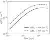Fig. C.1

CO density time evolution for a simulated cloud with A_v = 1 and T=35 K.

In Fig. C.1 we show the evolution of the CO number density as a function of time. When $n_{H_{2}} = 800 {cm}^{- 3}$ ${n_{{{\rm{H}}_2}}} = 800\,{\rm{c}}{{\rm{m}}^{ - 3}}$ , the CO abundance is consistently higher than that for $n_{H_{2}} = 600 {cm}^{- 3}$ ${{\rm{n}}_{{{\rm{H}}_2}}} = 600\,{\rm{c}}{{\rm{m}}^{ - 3}}$ , but the increase rate in n(CO) is essentially the same. The timescale required to reach the first maximum abundance of n(CO) is τ_CO ≈ 1 Myr for any n(H₂). When we induce a detectability cutoff at n_CO = 0.01 cm⁻³, then for n(H₂) = 600 cm⁻³, we obtain that τ_CO ≈ 1 Myr, while for n(H₂) = 800 cm⁻³, τ_CO ≈ 0.03 Myr. In order to be conservative, we considered a wide range of CO timescales, τ_CO = 0.03–1.0 Myr.

References

Andersson, B. G., & Potter, S. B. 2007, ApJ, 665, 369 [NASA ADS] [CrossRef] [Google Scholar]
André, P., Men’shchikov, A., Bontemps, S., et al. 2010, A&A, 518, L102 [CrossRef] [EDP Sciences] [Google Scholar]
Backer, D. C., & Chandran, B. D. G. 2000, AAS Meet. Abst., 197, 07.08 [NASA ADS] [Google Scholar]
Bailer-Jones, C. A. L., Rybizki, J., Fouesneau, M., Demleitner, M., & Andrae, R. 2021, AJ, 161, 147 [Google Scholar]
Beattie, J. R., & Federrath, C. 2020, MNRAS, 492, 668 [Google Scholar]
Beattie, J. R., Federrath, C., & Seta, A. 2020, MNRAS, 498, 1593 [Google Scholar]
Bellomi, E., Godard, B., Hennebelle, P., et al. 2020, A&A, 643, A36 [NASA ADS] [CrossRef] [EDP Sciences] [Google Scholar]
Bialy, S., & Sternberg, A. 2016, ApJ, 822, 83 [NASA ADS] [CrossRef] [Google Scholar]
Bialy, S., Burkhart, B., & Sternberg, A. 2017, ApJ, 843, 92 [NASA ADS] [CrossRef] [Google Scholar]
Bieging, J. H., Revelle, M., & Peters, W. L. 2014, ApJS, 214, 7 [NASA ADS] [CrossRef] [Google Scholar]
Bisbas, T. G., Tan, J. C., & Tanaka, K. E. I. 2021, MNRAS, 502, 2701 [CrossRef] [Google Scholar]
Blinov, D., Kiehlmann, S., Pavlidou, V., et al. 2021, MNRAS, 501, 3715 [NASA ADS] [CrossRef] [Google Scholar]
Bobylev, V. V., & Bajkova, A. T. 2021, Astron. Rep., 65, 498 [NASA ADS] [CrossRef] [Google Scholar]
Burgh, E. B., France, K., & McCandliss, S. R. 2007, ApJ, 658, 446 [NASA ADS] [CrossRef] [Google Scholar]
Burleigh, K. J., Bieging, J. H., Chromey, A., Kulesa, C., & Peters, W. L. 2013, ApJS, 209, 39 [Google Scholar]
Chandrasekhar, S., & Fermi, E. 1953, ApJ, 118, 113 [Google Scholar]
Chapman, N. L., Goldsmith, P. F., Pineda, J. L., et al. 2011, ApJ, 741, 21 [NASA ADS] [CrossRef] [Google Scholar]
Chen, C.-Y., & Ostriker, E. C. 2014, ApJ, 785, 69 [NASA ADS] [CrossRef] [Google Scholar]
Chen, C.-Y., Li, Z.-Y., King, P. K., & Fissel, L. M. 2017, ApJ, 847, 140 [NASA ADS] [CrossRef] [Google Scholar]
Chevance, M., Krumholz, M. R., McLeod, A. F., et al. 2022, ArXiv e-prints [arXiv:2203.09570] [Google Scholar]
Clark, S. E., Peek, J. E. G., & Putman, M. E. 2014, ApJ, 789, 82 [NASA ADS] [CrossRef] [Google Scholar]
Cox, N. L. J., Arzoumanian, D., André, P., et al. 2016, A&A, 590, A110 [NASA ADS] [CrossRef] [EDP Sciences] [Google Scholar]
Dame, T. M., Hartmann, D., & Thaddeus, P. 2001, ApJ, 547, 792 [Google Scholar]
Davis, L., Jr. 1951, Phys. Rev., 81, 890 [NASA ADS] [CrossRef] [Google Scholar]
Desai, K. M., Gwinn, C. R., & Diamond, P. J. 1994, Nature, 372, 754 [NASA ADS] [CrossRef] [Google Scholar]
Dubey, A., Fisher, R., Graziani, C., et al. 2008, ASP Conf. Ser., 385, 145 [NASA ADS] [Google Scholar]
Falceta-Gonçalves, D., Lazarian, A., & Kowal, G. 2008, ApJ, 679, 537 [Google Scholar]
Federman, S. R., Rawlings, J. M. C., Taylor, S. D., & Williams, D. A. 1996, MNRAS, 279, L41 [NASA ADS] [CrossRef] [Google Scholar]
Federrath, C., & Banerjee, S. 2015, MNRAS, 448, 3297 [NASA ADS] [CrossRef] [Google Scholar]
Federrath, C., Klessen, R. S., Iapichino, L., & Beattie, J. R. 2021, Nat. Astron., 5, 365 [NASA ADS] [CrossRef] [Google Scholar]
Foreman-Mackey, D. 2016, J. Open Source Softw., 1, 24 [Google Scholar]
Foreman-Mackey, D., Hogg, D. W., Lang, D., & Goodman, J. 2013, PASP, 125, 306 [Google Scholar]
Frisch, P. C., Berdyugin, A., Piirola, V., et al. 2015, ApJ, 814, 112 [NASA ADS] [CrossRef] [Google Scholar]
Fryxell, B., Olson, K., Ricker, P., et al. 2000, ApJS, 131, 273 [Google Scholar]
Gaia Collaboration (Brown, A. G. A., et al.) 2021, A&A, 649, A1 [NASA ADS] [CrossRef] [EDP Sciences] [Google Scholar]
Gillmon, K., Shull, J. M., Tumlinson, J., & Danforth, C. 2006, ApJ, 636, 891 [NASA ADS] [CrossRef] [Google Scholar]
Girichidis, P., Seifried, D., Naab, T., et al. 2018, MNRAS, 480, 3511 [NASA ADS] [CrossRef] [Google Scholar]
Glover, S. C. O., & Clark, P. C. 2012, MNRAS, 421, 116 [NASA ADS] [Google Scholar]
Glover, S. C. O., & Mac Low, M.-M. 2007a, ApJS, 169, 239 [NASA ADS] [CrossRef] [Google Scholar]
Glover, S. C. O., & Mac Low, M.-M. 2007b, ApJ, 659, 1317 [NASA ADS] [CrossRef] [Google Scholar]
Goldsmith, P. F. 2013, ApJ, 774, 134 [NASA ADS] [CrossRef] [Google Scholar]
Goldsmith, P. F., & Li, D. 2005, ApJ, 622, 938 [NASA ADS] [CrossRef] [Google Scholar]
Goldsmith, P. F., Li, D., & Krčo, M. 2007, ApJ, 654, 273 [NASA ADS] [CrossRef] [Google Scholar]
Goldsmith, P. F., Heyer, M., Narayanan, G., et al. 2008, ApJ, 680, 428 [Google Scholar]
Goldsmith, P. F., Pineda, J. L., Neufeld, D. A., et al. 2018, ApJ, 856, 96 [NASA ADS] [CrossRef] [Google Scholar]
Gong, M., Ostriker, E. C., & Wolfire, M. G. 2017, ApJ, 843, 38 [NASA ADS] [CrossRef] [Google Scholar]
Gong, M., Ostriker, E. C., & Kim, C.-G. 2018, ApJ, 858, 16 [Google Scholar]
Gong, M., Ostriker, E. C., Kim, C.-G., & Kim, J.-G. 2020, ApJ, 903, 142 [CrossRef] [Google Scholar]
Green, G. M., Schlafly, E. F., Finkbeiner, D., et al. 2018, MNRAS, 478, 651 [Google Scholar]
Grenier, I. A., Casandjian, J.-M., & Terrier, R. 2005, Science, 307, 1292 [Google Scholar]
Griffin, M. J., Abergel, A., Abreu, A., et al. 2010, A&A, 518, L3 [EDP Sciences] [Google Scholar]
Gudennavar, S. B., Bubbly, S. G., Preethi, K., & Murthy, J. 2012, ApJS, 199, 8 [NASA ADS] [CrossRef] [Google Scholar]
Hacar, A., Clark, S., Heitsch, F., et al. 2022, ArXiv e-prints [arXiv:2203.09562] [Google Scholar]
Heiles, C., & Troland, T. H. 2003, ApJS, 145, 329 [Google Scholar]
Heitsch, F., Zweibel, E. G., Mac Low, M.-M., Li, P., & Norman, M. L. 2001, ApJ, 561, 800 [Google Scholar]
Heyer, M., Gong, H., Ostriker, E., & Brunt, C. 2008, ApJ, 680, 420 [Google Scholar]
Heyer, M., Goldsmith, P. F., Yıldız, U. A., et al. 2016, MNRAS, 461, 3918 [NASA ADS] [CrossRef] [Google Scholar]
Higdon, J. C. 1984, ApJ, 285, 109 [Google Scholar]
Iwasaki, K., & Tomida, K. 2022, ApJ, 934, 174 [NASA ADS] [CrossRef] [Google Scholar]
Iwasaki, K., Tomida, K., Inoue, T., & Inutsuka, S.-I. 2019, ApJ, 873, 6 [NASA ADS] [CrossRef] [Google Scholar]
Kauffmann, J., Bertoldi, F., Bourke, T. L., Evans, N. J. I., & Lee, C. W. 2008, A&A, 487, 993 [NASA ADS] [CrossRef] [EDP Sciences] [Google Scholar]
King, O. G., Blinov, D., Ramaprakash, A. N., et al. 2014, MNRAS, 442, 1706 [NASA ADS] [CrossRef] [Google Scholar]
Lallement, R., Babusiaux, C., Vergely, J. L., et al. 2019, A&A, 625, A135 [NASA ADS] [CrossRef] [EDP Sciences] [Google Scholar]
Langer, W. D., & Penzias, A. A. 1990, ApJ, 357, 477 [Google Scholar]
Langer, W. D., Velusamy, T., Pineda, J. L., et al. 2010, A&A, 521, L17 [NASA ADS] [CrossRef] [EDP Sciences] [Google Scholar]
Leike, R. H., Glatzle, M., & Enßlin, T. A. 2020, A&A, 639, A138 [NASA ADS] [CrossRef] [EDP Sciences] [Google Scholar]
Le Petit, F., Nehmé, C., Le Bourlot, J., & Roueff, E. 2006, ApJS, 164, 506 [NASA ADS] [CrossRef] [Google Scholar]
Levrier, F., Le Petit, F., Hennebelle, P., et al. 2012, A&A, 544, A22 [NASA ADS] [CrossRef] [EDP Sciences] [Google Scholar]
Malinen, J., Juvela, M., Zahorecz, S., et al. 2014, A&A, 563, A125 [NASA ADS] [CrossRef] [EDP Sciences] [Google Scholar]
Malinen, J., Montier, L., Montillaud, J., et al. 2016, MNRAS, 460, 1934 [Google Scholar]
Meidt, S. E., Hughes, A., Dobbs, C. L., et al. 2015, ApJ, 806, 72 [NASA ADS] [CrossRef] [Google Scholar]
Milam, S. N., Savage, C., Brewster, M. A., Ziurys, L. M., & Wyckoff, S. 2005, ApJ, 634, 1126 [Google Scholar]
Miville-Deschênes, M. A., & Martin, P. G. 2007, A&A, 469, 189 [NASA ADS] [CrossRef] [EDP Sciences] [Google Scholar]
Miville-Deschênes, M. A., Joncas, G., Falgarone, E., & Boulanger, F. 2003, A&A, 411, 109 [NASA ADS] [CrossRef] [EDP Sciences] [Google Scholar]
Miville-Deschênes, M. A., Martin, P. G., Abergel, A., et al. 2010, A&A, 518, A104 [Google Scholar]
Mouschovias, T. C., Tassis, K., & Kunz, M. W. 2006, ApJ, 646, 1043 [Google Scholar]
Mouschovias, T. C., Ciolek, G. E., & Morton, S. A. 2011, MNRAS, 415, 1751 [NASA ADS] [CrossRef] [Google Scholar]
Murray, N. 2011, ApJ, 729, 133 [NASA ADS] [CrossRef] [Google Scholar]
Ostriker, E. C., Stone, J. M., & Gammie, C. F. 2001, ApJ, 546, 980 [Google Scholar]
Padoan, P., Goodman, A., Draine, B. T., et al. 2001, ApJ, 559, 1005 [Google Scholar]
Palmeirim, P., André, P., Kirk, J., et al. 2013, A&A, 550, A38 [NASA ADS] [CrossRef] [EDP Sciences] [Google Scholar]
Panopoulou, G., Tassis, K., Blinov, D., et al. 2015, MNRAS, 452, 715 [Google Scholar]
Panopoulou, G. V., Psaradaki, I., & Tassis, K. 2016, MNRAS, 462, 1517 [Google Scholar]
Panopoulou, G. V., Hensley, B. S., Skalidis, R., Blinov, D., & Tassis, K. 2019, A&A, 624, L8 [NASA ADS] [CrossRef] [EDP Sciences] [Google Scholar]
Panopoulou, G. V., Clark, S. E., Hacar, A., et al. 2022, A&A, 657, L13 [NASA ADS] [CrossRef] [EDP Sciences] [Google Scholar]
Paradis, D., Dobashi, K., Shimoikura, T., et al. 2012, A&A, 543, A103 [NASA ADS] [CrossRef] [EDP Sciences] [Google Scholar]
Paranjpye, D., Mahabal, A., Ramaprakash, A. N., et al. 2020, MNRAS, 491, 5151 [NASA ADS] [CrossRef] [Google Scholar]
Pardi, A., Girichidis, P., Naab, T., et al. 2017, MNRAS, 465, 4611 [CrossRef] [Google Scholar]
Pattle, K., Ward-Thompson, D., Berry, D., et al. 2017, ApJ, 846, 122 [Google Scholar]
Pelgrims, V., Panopoulou, G. V., Tassis, K., et al. 2023, A&A, 670, A164 [NASA ADS] [CrossRef] [EDP Sciences] [Google Scholar]
Pety, J., Liszt, H. S., & Lucas, R. 2011, EAS Publ. Ser., 52, 151 [NASA ADS] [CrossRef] [EDP Sciences] [Google Scholar]
Pineda, J. L., Goldsmith, P. F., Chapman, N., et al. 2010, ApJ, 721, 686 [NASA ADS] [CrossRef] [Google Scholar]
Pineda, J. L., Langer, W. D., Velusamy, T., & Goldsmith, P. F. 2013, A&A, 554, A103 [CrossRef] [EDP Sciences] [Google Scholar]
Planck Collaboration XII. 2020, A&A, 641, A12 [NASA ADS] [CrossRef] [EDP Sciences] [Google Scholar]
Planck Collaboration Int. XXXV. 2016, A&A, 586, A138 [NASA ADS] [CrossRef] [EDP Sciences] [Google Scholar]
Plaszczynski, S., Montier, L., Levrier, F., & Tristram, M. 2014, MNRAS, 439, 4048 [NASA ADS] [CrossRef] [Google Scholar]
Pudritz, R. E., & Kevlahan, N. K. R. 2013, Philos. Trans. Roy. Soc. Lond. A, 371, 20120248 [NASA ADS] [Google Scholar]
Ramaprakash, A. N., Rajarshi, C. V., Das, H. K., et al. 2019, MNRAS, 485, 2355 [NASA ADS] [CrossRef] [Google Scholar]
Seifried, D., & Walch, S. 2016, MNRAS, 459, L11 [NASA ADS] [CrossRef] [Google Scholar]
Seifried, D., Walch, S., Girichidis, P., et al. 2017, MNRAS, 472, 4797 [NASA ADS] [CrossRef] [Google Scholar]
Seifried, D., Beuther, H., Walch, S., et al. 2021, MNRAS, 000, 1 [Google Scholar]
Shaikh, D., & Zank, G. P. 2007, ApJ, 656, L17 [NASA ADS] [CrossRef] [Google Scholar]
Sheffer, Y., Rogers, M., Federman, S. R., et al. 2008, ApJ, 687, 1075 [Google Scholar]
Skalidis, R., & Tassis, K. 2021, A&A, 647, A186 [NASA ADS] [CrossRef] [EDP Sciences] [Google Scholar]
Skalidis, R., Panopoulou, G. V., Tassis, K., et al. 2018, A&A, 616, A52 [NASA ADS] [CrossRef] [EDP Sciences] [Google Scholar]
Skalidis, R., Sternberg, J., Beattie, J. R., Pavlidou, V., & Tassis, K. 2021, A&A, 656, A118 [NASA ADS] [CrossRef] [EDP Sciences] [Google Scholar]
Skalidis, R., Tassis, K., Panopoulou, G. V., et al. 2022, A&A, 665, A77 [NASA ADS] [CrossRef] [EDP Sciences] [Google Scholar]
Snow, T. P., & McCall, B. J. 2006, ARA&A, 44, 367 [NASA ADS] [CrossRef] [Google Scholar]
Sternberg, A., & Dalgarno, A. 1995, ApJS, 99, 565 [NASA ADS] [CrossRef] [Google Scholar]
Stewart, M., & Federrath, C. 2022, MNRAS, 509, 5237 [Google Scholar]
Szűcs, L., Glover, S. C. O., & Klessen, R. S. 2014, MNRAS, 445, 4055 [CrossRef] [Google Scholar]
Tassis, K., & Mouschovias, T. C. 2004, ApJ, 616, 283 [Google Scholar]
Tassis, K., Willacy, K., Yorke, H. W., & Turner, N. J. 2014, MNRAS, 445, L56 [CrossRef] [Google Scholar]
Tritsis, A., & Tassis, K. 2016, MNRAS, 462, 3602 [Google Scholar]
Tritsis, A., & Tassis, K. 2018, Science, 360, 635 [Google Scholar]
Tritsis, A., Tassis, K., & Willacy, K. 2016, MNRAS, 458, 789 [CrossRef] [Google Scholar]
Tritsis, A., Federrath, C., Schneider, N., & Tassis, K. 2018, MNRAS, 481, 5275 [Google Scholar]
Tritsis, A., Federrath, C., & Pavlidou, V. 2019, ApJ, 873, 38 [NASA ADS] [CrossRef] [Google Scholar]
Tritsis, A., Bouzelou, F., Skalidis, R., et al. 2022a, MNRAS, 514, 3593 [NASA ADS] [CrossRef] [Google Scholar]
Tritsis, A., Federrath, C., Willacy, K., & Tassis, K. 2022b, MNRAS, 510, 4420 [NASA ADS] [CrossRef] [Google Scholar]
Vaillancourt, J. E. 2006, PASP, 118, 1340 [Google Scholar]
Valdivia, V., Hennebelle, P., Gérin, M., & Lesaffre, P. 2016, A&A, 587, A76 [NASA ADS] [CrossRef] [EDP Sciences] [Google Scholar]
van der Tak, F. F. S., Black, J. H., Schöier, F. L., Jansen, D. J., & van Dishoeck, E. F. 2007, A&A, 468, 627 [NASA ADS] [CrossRef] [EDP Sciences] [Google Scholar]
van Dishoeck, E. F., & Black, J. H. 1988, ApJ, 334, 771 [Google Scholar]
Visser, R., van Dishoeck, E. F., & Black, J. H. 2009, A&A, 503, 323 [NASA ADS] [CrossRef] [EDP Sciences] [Google Scholar]
Walch, S., Girichidis, P., Naab, T., et al. 2015, MNRAS, 454, 238 [Google Scholar]
Watson, W. D., Anicich, V. G., & Huntress, W. T. J., 1976, ApJ, 205, L165 [NASA ADS] [CrossRef] [Google Scholar]
Xu, S., Ji, S., & Lazarian, A. 2019, ApJ, 878, 157 [CrossRef] [Google Scholar]
Zucker, C., Goodman, A., Alves, J., et al. 2021, ApJ, 919, 35 [NASA ADS] [CrossRef] [Google Scholar]

¹

http://skinakas.physics.uoc.gr

All Tables

Table 1

Region parameters.

In the text

All Figures

	Fig. 1 Large-scale view of the Polaris Flare as observed with the Spire instrument of the Herschel observatory at 500 µm. The magenta polygon shows the CO surveyed region, and blue contours show the smoothed integrated CO (J = 2−1) intensity emission at 2.5 and 4 K km s⁻¹.
In the text

	Fig. 2 Zoomed-in view toward the striation region. Optical polarization segments (red lines) are overplotted on the dust continuum emission map of the Polaris Flare as observed with Herschel at 500 µm. A line is shown for scale in the top left corner of the figure, corresponding to a degree of polarization of p = 2%. Blue contours correspond to the ¹²CO integrated intensity as in Fig. 1.
In the text

	Fig. 3 Integrated intensity maps of CO (J = 2−1). The velocity integration interval is shown in the top left corner of each panel. Velocities are in km s⁻¹.
In the text

	Fig. 4 CO integrated intensity moment map at native resolution, without any filtering or masking. Cyan box-shaped regions are defined by the positions at which we detected the ¹³CO (J = 2−1) line. Inset panels show the mean spectra of ¹²CO (magenta) and ¹³CO (blue) within the cyan boxes. The intensity of the ¹³CO emission is approximately an order of magnitude lower than ¹²CO.
In the text

Fig. 5

¹²CO (J = 2−1) moment maps smoothed at a resolution of 2.57′. The circular beam in the left corner of each panel shows the Gaussian kernel used for smoothing the data. Magenta segments show the POS magnetic field orientation as traced by optical dust polarization. A scale segment is shown in the upper left corner in each panel. Pixels with a total CO intensity lower than 1.1 (K km s⁻¹) have been masked out. The dotted black rectangle defines the boundaries of region I, and the solid polygon defines region II. The black labels (I, II) are the region identifiers. Top left panel: Intensity (zero-moment) map of CO. Upper right panel: Intensity profiles along the white line shown in the I₀ map. The left vertical axis corresponds to the CO (J = 2−1) integrated intensity. The right vertical axis corresponds to the dust intensity of the three Herschel bands of the SPIRE instrument. The wavelength of each band is shown in the legend. The quasiperiodicity of the CO intensity fluctuations is prominent across this line. The wavelength of the pattern is ~1 pc. Dust intensity profiles are more complex than the CO profile, showing several subparsec features. Bottom left panel: Centroid velocity (I₁, first moment) map of CO. Right panel: Velocity dispersion of CO ( $\sqrt{I_{2}},$ $\sqrt {{I_2}} ,$ square root of the second-moment map).

In the text

	Fig. 6 Averaged CO spectra toward regions I and II. The width of each bin is equal to the spectral resolution. Colored lines correspond to Gaussian fits. The mean velocities of regions I and II are −0.80, and −2.22 km s⁻¹, respectively. The FWHM line widths in regions I and II are 1.39 and 2.61 km s⁻¹, respectively.
In the text

	Fig. 7 Normalized distributions of polarization angles for both regions. The size of each bin has been optimized using Bayesian analysis from astropy, in order to reflect the intrinsic shape of each distribution.
In the text

	Fig. 8 1D, and 2D marginalized posterior distributions of θ₀, and δθ₀ for regions I (left panel) and II (right panel). These plots were produced with the corner plot function of Foreman-Mackey (2016).
In the text

	Fig. A.1 Images showing blended objects used for the training of the CNN. The size of each image is 64 × 64 pixel.
In the text

	Fig. A.2 Normalized confusion matrices of the three neural networks trained for the identification of blended stars in polarization images. The probability of true positives and false negatives is higher than 0.9 for every model. The probability of true negatives and false positives is lower than 0.1 for every model.
In the text

	Fig. B.1 CO vs. H₂ column density. Black points correspond to archival data. The solid blue lines are 7000 realizations extracted from the posterior distributions of the Bayesian fitting. The dotted black line corresponds to 10⁻⁴ $N_{H_{2}}$ ${{\rm{N}}_{{{\rm{H}}_2}}}$ , which corresponds to clouds in which essentially all carbon is in the form of CO.
In the text

	Fig. B.2 Results of the PDR modeling for A_v = 1. Upper panel: Kinetic temperature vs. A_v for different gas densities and UV intensities (G). Lower panel: Densities of H₂ and CO vs. A_v.
In the text

	Fig. C.1 CO density time evolution for a simulated cloud with A_v = 1 and T=35 K.
In the text

Current usage metrics show cumulative count of Article Views (full-text article views including HTML views, PDF and ePub downloads, according to the available data) and Abstracts Views on Vision4Press platform.

Data correspond to usage on the plateform after 2015. The current usage metrics is available 48-96 hours after online publication and is updated daily on week days.

Initial download of the metrics may take a while.

[1] Andersson, B. G., & Potter, S. B. 2007, ApJ, 665, 369 [NASA ADS] [CrossRef] [Google Scholar]

[2] André, P., Men’shchikov, A., Bontemps, S., et al. 2010, A&A, 518, L102 [CrossRef] [EDP Sciences] [Google Scholar]

[3] Backer, D. C., & Chandran, B. D. G. 2000, AAS Meet. Abst., 197, 07.08 [NASA ADS] [Google Scholar]

[4] Bailer-Jones, C. A. L., Rybizki, J., Fouesneau, M., Demleitner, M., & Andrae, R. 2021, AJ, 161, 147 [Google Scholar]

[5] Beattie, J. R., & Federrath, C. 2020, MNRAS, 492, 668 [Google Scholar]

[6] Beattie, J. R., Federrath, C., & Seta, A. 2020, MNRAS, 498, 1593 [Google Scholar]

[7] Bellomi, E., Godard, B., Hennebelle, P., et al. 2020, A&A, 643, A36 [NASA ADS] [CrossRef] [EDP Sciences] [Google Scholar]

[8] Bialy, S., & Sternberg, A. 2016, ApJ, 822, 83 [NASA ADS] [CrossRef] [Google Scholar]

[9] Bialy, S., Burkhart, B., & Sternberg, A. 2017, ApJ, 843, 92 [NASA ADS] [CrossRef] [Google Scholar]

[10] Bieging, J. H., Revelle, M., & Peters, W. L. 2014, ApJS, 214, 7 [NASA ADS] [CrossRef] [Google Scholar]

[11] Bisbas, T. G., Tan, J. C., & Tanaka, K. E. I. 2021, MNRAS, 502, 2701 [CrossRef] [Google Scholar]

[12] Blinov, D., Kiehlmann, S., Pavlidou, V., et al. 2021, MNRAS, 501, 3715 [NASA ADS] [CrossRef] [Google Scholar]

[13] Bobylev, V. V., & Bajkova, A. T. 2021, Astron. Rep., 65, 498 [NASA ADS] [CrossRef] [Google Scholar]

[14] Burgh, E. B., France, K., & McCandliss, S. R. 2007, ApJ, 658, 446 [NASA ADS] [CrossRef] [Google Scholar]

[15] Burleigh, K. J., Bieging, J. H., Chromey, A., Kulesa, C., & Peters, W. L. 2013, ApJS, 209, 39 [Google Scholar]

[16] Chandrasekhar, S., & Fermi, E. 1953, ApJ, 118, 113 [Google Scholar]

[17] Chapman, N. L., Goldsmith, P. F., Pineda, J. L., et al. 2011, ApJ, 741, 21 [NASA ADS] [CrossRef] [Google Scholar]

[18] Chen, C.-Y., & Ostriker, E. C. 2014, ApJ, 785, 69 [NASA ADS] [CrossRef] [Google Scholar]

[19] Chen, C.-Y., Li, Z.-Y., King, P. K., & Fissel, L. M. 2017, ApJ, 847, 140 [NASA ADS] [CrossRef] [Google Scholar]

[20] Chevance, M., Krumholz, M. R., McLeod, A. F., et al. 2022, ArXiv e-prints [arXiv:2203.09570] [Google Scholar]

[21] Clark, S. E., Peek, J. E. G., & Putman, M. E. 2014, ApJ, 789, 82 [NASA ADS] [CrossRef] [Google Scholar]

[22] Cox, N. L. J., Arzoumanian, D., André, P., et al. 2016, A&A, 590, A110 [NASA ADS] [CrossRef] [EDP Sciences] [Google Scholar]

[23] Dame, T. M., Hartmann, D., & Thaddeus, P. 2001, ApJ, 547, 792 [Google Scholar]

[24] Davis, L., Jr. 1951, Phys. Rev., 81, 890 [NASA ADS] [CrossRef] [Google Scholar]

[25] Desai, K. M., Gwinn, C. R., & Diamond, P. J. 1994, Nature, 372, 754 [NASA ADS] [CrossRef] [Google Scholar]

[26] Dubey, A., Fisher, R., Graziani, C., et al. 2008, ASP Conf. Ser., 385, 145 [NASA ADS] [Google Scholar]

[27] Falceta-Gonçalves, D., Lazarian, A., & Kowal, G. 2008, ApJ, 679, 537 [Google Scholar]

[28] Federman, S. R., Rawlings, J. M. C., Taylor, S. D., & Williams, D. A. 1996, MNRAS, 279, L41 [NASA ADS] [CrossRef] [Google Scholar]

[29] Federrath, C., & Banerjee, S. 2015, MNRAS, 448, 3297 [NASA ADS] [CrossRef] [Google Scholar]

[30] Federrath, C., Klessen, R. S., Iapichino, L., & Beattie, J. R. 2021, Nat. Astron., 5, 365 [NASA ADS] [CrossRef] [Google Scholar]

[31] Foreman-Mackey, D. 2016, J. Open Source Softw., 1, 24 [Google Scholar]

[32] Foreman-Mackey, D., Hogg, D. W., Lang, D., & Goodman, J. 2013, PASP, 125, 306 [Google Scholar]

[33] Frisch, P. C., Berdyugin, A., Piirola, V., et al. 2015, ApJ, 814, 112 [NASA ADS] [CrossRef] [Google Scholar]

[34] Fryxell, B., Olson, K., Ricker, P., et al. 2000, ApJS, 131, 273 [Google Scholar]

[35] Gaia Collaboration (Brown, A. G. A., et al.) 2021, A&A, 649, A1 [NASA ADS] [CrossRef] [EDP Sciences] [Google Scholar]

[36] Gillmon, K., Shull, J. M., Tumlinson, J., & Danforth, C. 2006, ApJ, 636, 891 [NASA ADS] [CrossRef] [Google Scholar]

[37] Girichidis, P., Seifried, D., Naab, T., et al. 2018, MNRAS, 480, 3511 [NASA ADS] [CrossRef] [Google Scholar]

[38] Glover, S. C. O., & Clark, P. C. 2012, MNRAS, 421, 116 [NASA ADS] [Google Scholar]

[39] Glover, S. C. O., & Mac Low, M.-M. 2007a, ApJS, 169, 239 [NASA ADS] [CrossRef] [Google Scholar]

[40] Glover, S. C. O., & Mac Low, M.-M. 2007b, ApJ, 659, 1317 [NASA ADS] [CrossRef] [Google Scholar]

[41] Goldsmith, P. F. 2013, ApJ, 774, 134 [NASA ADS] [CrossRef] [Google Scholar]

[42] Goldsmith, P. F., & Li, D. 2005, ApJ, 622, 938 [NASA ADS] [CrossRef] [Google Scholar]

[43] Goldsmith, P. F., Li, D., & Krčo, M. 2007, ApJ, 654, 273 [NASA ADS] [CrossRef] [Google Scholar]

[44] Goldsmith, P. F., Heyer, M., Narayanan, G., et al. 2008, ApJ, 680, 428 [Google Scholar]

[45] Goldsmith, P. F., Pineda, J. L., Neufeld, D. A., et al. 2018, ApJ, 856, 96 [NASA ADS] [CrossRef] [Google Scholar]

[46] Gong, M., Ostriker, E. C., & Wolfire, M. G. 2017, ApJ, 843, 38 [NASA ADS] [CrossRef] [Google Scholar]

[47] Gong, M., Ostriker, E. C., & Kim, C.-G. 2018, ApJ, 858, 16 [Google Scholar]

[48] Gong, M., Ostriker, E. C., Kim, C.-G., & Kim, J.-G. 2020, ApJ, 903, 142 [CrossRef] [Google Scholar]

[49] Green, G. M., Schlafly, E. F., Finkbeiner, D., et al. 2018, MNRAS, 478, 651 [Google Scholar]

[50] Grenier, I. A., Casandjian, J.-M., & Terrier, R. 2005, Science, 307, 1292 [Google Scholar]

[51] Griffin, M. J., Abergel, A., Abreu, A., et al. 2010, A&A, 518, L3 [EDP Sciences] [Google Scholar]

[52] Gudennavar, S. B., Bubbly, S. G., Preethi, K., & Murthy, J. 2012, ApJS, 199, 8 [NASA ADS] [CrossRef] [Google Scholar]

[53] Hacar, A., Clark, S., Heitsch, F., et al. 2022, ArXiv e-prints [arXiv:2203.09562] [Google Scholar]

[54] Heiles, C., & Troland, T. H. 2003, ApJS, 145, 329 [Google Scholar]

[55] Heitsch, F., Zweibel, E. G., Mac Low, M.-M., Li, P., & Norman, M. L. 2001, ApJ, 561, 800 [Google Scholar]

[56] Heyer, M., Gong, H., Ostriker, E., & Brunt, C. 2008, ApJ, 680, 420 [Google Scholar]

[57] Heyer, M., Goldsmith, P. F., Yıldız, U. A., et al. 2016, MNRAS, 461, 3918 [NASA ADS] [CrossRef] [Google Scholar]

[58] Higdon, J. C. 1984, ApJ, 285, 109 [Google Scholar]

[59] Iwasaki, K., & Tomida, K. 2022, ApJ, 934, 174 [NASA ADS] [CrossRef] [Google Scholar]

[60] Iwasaki, K., Tomida, K., Inoue, T., & Inutsuka, S.-I. 2019, ApJ, 873, 6 [NASA ADS] [CrossRef] [Google Scholar]

[61] Kauffmann, J., Bertoldi, F., Bourke, T. L., Evans, N. J. I., & Lee, C. W. 2008, A&A, 487, 993 [NASA ADS] [CrossRef] [EDP Sciences] [Google Scholar]

[62] King, O. G., Blinov, D., Ramaprakash, A. N., et al. 2014, MNRAS, 442, 1706 [NASA ADS] [CrossRef] [Google Scholar]

[63] Lallement, R., Babusiaux, C., Vergely, J. L., et al. 2019, A&A, 625, A135 [NASA ADS] [CrossRef] [EDP Sciences] [Google Scholar]

[64] Langer, W. D., & Penzias, A. A. 1990, ApJ, 357, 477 [Google Scholar]

[65] Langer, W. D., Velusamy, T., Pineda, J. L., et al. 2010, A&A, 521, L17 [NASA ADS] [CrossRef] [EDP Sciences] [Google Scholar]

[66] Leike, R. H., Glatzle, M., & Enßlin, T. A. 2020, A&A, 639, A138 [NASA ADS] [CrossRef] [EDP Sciences] [Google Scholar]

[67] Le Petit, F., Nehmé, C., Le Bourlot, J., & Roueff, E. 2006, ApJS, 164, 506 [NASA ADS] [CrossRef] [Google Scholar]

[68] Levrier, F., Le Petit, F., Hennebelle, P., et al. 2012, A&A, 544, A22 [NASA ADS] [CrossRef] [EDP Sciences] [Google Scholar]

[69] Malinen, J., Juvela, M., Zahorecz, S., et al. 2014, A&A, 563, A125 [NASA ADS] [CrossRef] [EDP Sciences] [Google Scholar]

[70] Malinen, J., Montier, L., Montillaud, J., et al. 2016, MNRAS, 460, 1934 [Google Scholar]

[71] Meidt, S. E., Hughes, A., Dobbs, C. L., et al. 2015, ApJ, 806, 72 [NASA ADS] [CrossRef] [Google Scholar]

[72] Milam, S. N., Savage, C., Brewster, M. A., Ziurys, L. M., & Wyckoff, S. 2005, ApJ, 634, 1126 [Google Scholar]

[73] Miville-Deschênes, M. A., & Martin, P. G. 2007, A&A, 469, 189 [NASA ADS] [CrossRef] [EDP Sciences] [Google Scholar]

[74] Miville-Deschênes, M. A., Joncas, G., Falgarone, E., & Boulanger, F. 2003, A&A, 411, 109 [NASA ADS] [CrossRef] [EDP Sciences] [Google Scholar]

[75] Miville-Deschênes, M. A., Martin, P. G., Abergel, A., et al. 2010, A&A, 518, A104 [Google Scholar]

[76] Mouschovias, T. C., Tassis, K., & Kunz, M. W. 2006, ApJ, 646, 1043 [Google Scholar]

[77] Mouschovias, T. C., Ciolek, G. E., & Morton, S. A. 2011, MNRAS, 415, 1751 [NASA ADS] [CrossRef] [Google Scholar]

[78] Murray, N. 2011, ApJ, 729, 133 [NASA ADS] [CrossRef] [Google Scholar]

[79] Ostriker, E. C., Stone, J. M., & Gammie, C. F. 2001, ApJ, 546, 980 [Google Scholar]

[80] Padoan, P., Goodman, A., Draine, B. T., et al. 2001, ApJ, 559, 1005 [Google Scholar]

[81] Palmeirim, P., André, P., Kirk, J., et al. 2013, A&A, 550, A38 [NASA ADS] [CrossRef] [EDP Sciences] [Google Scholar]

[82] Panopoulou, G., Tassis, K., Blinov, D., et al. 2015, MNRAS, 452, 715 [Google Scholar]

[83] Panopoulou, G. V., Psaradaki, I., & Tassis, K. 2016, MNRAS, 462, 1517 [Google Scholar]

[84] Panopoulou, G. V., Hensley, B. S., Skalidis, R., Blinov, D., & Tassis, K. 2019, A&A, 624, L8 [NASA ADS] [CrossRef] [EDP Sciences] [Google Scholar]

[85] Panopoulou, G. V., Clark, S. E., Hacar, A., et al. 2022, A&A, 657, L13 [NASA ADS] [CrossRef] [EDP Sciences] [Google Scholar]

[86] Paradis, D., Dobashi, K., Shimoikura, T., et al. 2012, A&A, 543, A103 [NASA ADS] [CrossRef] [EDP Sciences] [Google Scholar]

[87] Paranjpye, D., Mahabal, A., Ramaprakash, A. N., et al. 2020, MNRAS, 491, 5151 [NASA ADS] [CrossRef] [Google Scholar]

[88] Pardi, A., Girichidis, P., Naab, T., et al. 2017, MNRAS, 465, 4611 [CrossRef] [Google Scholar]

[89] Pattle, K., Ward-Thompson, D., Berry, D., et al. 2017, ApJ, 846, 122 [Google Scholar]

[90] Pelgrims, V., Panopoulou, G. V., Tassis, K., et al. 2023, A&A, 670, A164 [NASA ADS] [CrossRef] [EDP Sciences] [Google Scholar]

[91] Pety, J., Liszt, H. S., & Lucas, R. 2011, EAS Publ. Ser., 52, 151 [NASA ADS] [CrossRef] [EDP Sciences] [Google Scholar]

[92] Pineda, J. L., Goldsmith, P. F., Chapman, N., et al. 2010, ApJ, 721, 686 [NASA ADS] [CrossRef] [Google Scholar]

[93] Pineda, J. L., Langer, W. D., Velusamy, T., & Goldsmith, P. F. 2013, A&A, 554, A103 [CrossRef] [EDP Sciences] [Google Scholar]

[94] Planck Collaboration XII. 2020, A&A, 641, A12 [NASA ADS] [CrossRef] [EDP Sciences] [Google Scholar]

[95] Planck Collaboration Int. XXXV. 2016, A&A, 586, A138 [NASA ADS] [CrossRef] [EDP Sciences] [Google Scholar]

[96] Plaszczynski, S., Montier, L., Levrier, F., & Tristram, M. 2014, MNRAS, 439, 4048 [NASA ADS] [CrossRef] [Google Scholar]

[97] Pudritz, R. E., & Kevlahan, N. K. R. 2013, Philos. Trans. Roy. Soc. Lond. A, 371, 20120248 [NASA ADS] [Google Scholar]

[98] Ramaprakash, A. N., Rajarshi, C. V., Das, H. K., et al. 2019, MNRAS, 485, 2355 [NASA ADS] [CrossRef] [Google Scholar]

[99] Seifried, D., & Walch, S. 2016, MNRAS, 459, L11 [NASA ADS] [CrossRef] [Google Scholar]

[100] Seifried, D., Walch, S., Girichidis, P., et al. 2017, MNRAS, 472, 4797 [NASA ADS] [CrossRef] [Google Scholar]

[101] Seifried, D., Beuther, H., Walch, S., et al. 2021, MNRAS, 000, 1 [Google Scholar]

[102] Shaikh, D., & Zank, G. P. 2007, ApJ, 656, L17 [NASA ADS] [CrossRef] [Google Scholar]

[103] Sheffer, Y., Rogers, M., Federman, S. R., et al. 2008, ApJ, 687, 1075 [Google Scholar]

[104] Skalidis, R., & Tassis, K. 2021, A&A, 647, A186 [NASA ADS] [CrossRef] [EDP Sciences] [Google Scholar]

[105] Skalidis, R., Panopoulou, G. V., Tassis, K., et al. 2018, A&A, 616, A52 [NASA ADS] [CrossRef] [EDP Sciences] [Google Scholar]

[106] Skalidis, R., Sternberg, J., Beattie, J. R., Pavlidou, V., & Tassis, K. 2021, A&A, 656, A118 [NASA ADS] [CrossRef] [EDP Sciences] [Google Scholar]

[107] Skalidis, R., Tassis, K., Panopoulou, G. V., et al. 2022, A&A, 665, A77 [NASA ADS] [CrossRef] [EDP Sciences] [Google Scholar]

[108] Snow, T. P., & McCall, B. J. 2006, ARA&A, 44, 367 [NASA ADS] [CrossRef] [Google Scholar]

[109] Sternberg, A., & Dalgarno, A. 1995, ApJS, 99, 565 [NASA ADS] [CrossRef] [Google Scholar]

[110] Stewart, M., & Federrath, C. 2022, MNRAS, 509, 5237 [Google Scholar]

[111] Szűcs, L., Glover, S. C. O., & Klessen, R. S. 2014, MNRAS, 445, 4055 [CrossRef] [Google Scholar]

[112] Tassis, K., & Mouschovias, T. C. 2004, ApJ, 616, 283 [Google Scholar]

[113] Tassis, K., Willacy, K., Yorke, H. W., & Turner, N. J. 2014, MNRAS, 445, L56 [CrossRef] [Google Scholar]

[114] Tritsis, A., & Tassis, K. 2016, MNRAS, 462, 3602 [Google Scholar]

[115] Tritsis, A., & Tassis, K. 2018, Science, 360, 635 [Google Scholar]

[116] Tritsis, A., Tassis, K., & Willacy, K. 2016, MNRAS, 458, 789 [CrossRef] [Google Scholar]

[117] Tritsis, A., Federrath, C., Schneider, N., & Tassis, K. 2018, MNRAS, 481, 5275 [Google Scholar]

[118] Tritsis, A., Federrath, C., & Pavlidou, V. 2019, ApJ, 873, 38 [NASA ADS] [CrossRef] [Google Scholar]

[119] Tritsis, A., Bouzelou, F., Skalidis, R., et al. 2022a, MNRAS, 514, 3593 [NASA ADS] [CrossRef] [Google Scholar]

[120] Tritsis, A., Federrath, C., Willacy, K., & Tassis, K. 2022b, MNRAS, 510, 4420 [NASA ADS] [CrossRef] [Google Scholar]

[121] Vaillancourt, J. E. 2006, PASP, 118, 1340 [Google Scholar]

[122] Valdivia, V., Hennebelle, P., Gérin, M., & Lesaffre, P. 2016, A&A, 587, A76 [NASA ADS] [CrossRef] [EDP Sciences] [Google Scholar]

[123] van der Tak, F. F. S., Black, J. H., Schöier, F. L., Jansen, D. J., & van Dishoeck, E. F. 2007, A&A, 468, 627 [NASA ADS] [CrossRef] [EDP Sciences] [Google Scholar]

[124] van Dishoeck, E. F., & Black, J. H. 1988, ApJ, 334, 771 [Google Scholar]

[125] Visser, R., van Dishoeck, E. F., & Black, J. H. 2009, A&A, 503, 323 [NASA ADS] [CrossRef] [EDP Sciences] [Google Scholar]

[126] Walch, S., Girichidis, P., Naab, T., et al. 2015, MNRAS, 454, 238 [Google Scholar]