| Issue |
A&A
Volume 665, September 2022
|
|
|---|---|---|
| Article Number | A77 | |
| Number of page(s) | 24 | |
| Section | Interstellar and circumstellar matter | |
| DOI | https://doi.org/10.1051/0004-6361/202142512 | |
| Published online | 14 September 2022 | |
HI-H2 transition: Exploring the role of the magnetic field
A case study toward the Ursa Major cirrus★
1
Department of Physics & ITCP, University of Crete,
GR-70013
Heraklion, Greece
e-mail: This email address is being protected from spambots. You need JavaScript enabled to view it.
2
Institute of Astrophysics, Foundation for Research and Technology-Hellas,
Vasilika Vouton,
70013
Heraklion, Greece
3
California Institute of Technology,
MC249-17, 1200 East California Boulevard,
Pasadena, CA
91125, USA
4
Jet Propulsion Laboratory, California Institute of Technology,
4800 Oak Grove Drive,
Pasadena, CA
91109-8099, USA
5
Max-Planck-Institut für Radioastronomie,
Auf dem Hügel 69,
53121
Bonn, Germany
6
Purple Mountain Observatory & Key Laboratory for Radio Astronomy, Chinese Academy of Sciences,
10 Yuanhua Road,
210033
Nanjing, PR China
Received:
22
October
2021
Accepted:
27
May
2022
Abstract
Context. Atomic gas in the diffuse interstellar medium (ISM) is organized in filamentary structures. These structures usually host cold and dense molecular clumps. The Galactic magnetic field is considered to play an important role in the formation of these clumps.
Aims. Our goal is to explore the role of the magnetic field in the HI-H2 transition process.
Methods. We targeted a diffuse ISM filamentary cloud toward the Ursa Major cirrus where gas transitions from atomic to molecular. We probed the magnetic field properties of the cloud with optical polarization observations. We performed multiwavelength spectroscopic observations of different species in order to probe the gas phase properties of the cloud. We observed the CO (J = 1−0) and (J = 2−1) lines in order to probe the molecular content of the cloud. We also obtained observations of the [C ii] 157.6µm emission line in order to trace the CO-dark H2 gas and estimate the mean volume density of the cloud.
Results. We identified two distinct subregions within the cloud. One of the regions is mostly atomic, while the other is dominated by molecular gas, although most of it is CO-dark. The estimated plane-of-the-sky magnetic field strength between the two regions remains constant within uncertainties and lies in the range 13–30 µG. The total magnetic field strength does not scale with density. This implies that gas is compressed along the field lines. We also found that turbulence is trans-Alfvénic, with MA ≈ 1. In the molecular region, we detected an asymmetric CO clump whose minor axis is closer, with a 24° deviation, to the mean magnetic field orientation than the angle of its major axis. The H i velocity gradients are in general perpendicular to the mean magnetic field orientation except for the region close to the CO clump, where they tend to become parallel. This phenomenon is likely related to gas undergoing gravitational infall. The magnetic field morphology of the target cloud is parallel to the H i column density structure of the cloud in the atomic region, while it tends to become perpendicular to the H i structure in the molecular region. On the other hand, the magnetic field morphology seems to form a smaller offset angle with the total column density shape (including both atomic and molecular gas) of this transition cloud.
Conclusions. In the target cloud where the H i–H2 transition takes place, turbulence is trans-Alfvénic, and hence the magnetic field plays an important role in the cloud dynamics. Atomic gas probably accumulates preferentially along the magnetic field lines and creates overdensities where molecular gas can form. The magnetic field morphology is probed better by the total column density shape of the cloud, and not its H i column density shape.
Key words: polarization / ISM: magnetic fields / ISM: individual objects: North Celestial Pole Loop (except planetary nebulae) / ISM: abundances / ISM: clouds / ISM: molecules
Polarization and CO data are only available in electronic form at the CDS via anonymous ftp to cdsarc.u-strasbg.fr (130.79.128.5) or via http://cdsarc.u-strasbg.fr/viz-bin/cat/J/A+A/665/A77
© R. Skalidis et al. 2022
 Open Access article, published by EDP Sciences, under the terms of the Creative Commons Attribution License (https://creativecommons.org/licenses/by/4.0), which permits unrestricted use, distribution, and reproduction in any medium, provided the original work is properly cited.
This article is published in open access under the Subscribe-to-Open model. This email address is being protected from spambots. You need JavaScript enabled to view it. to support open access publication.
1 Introduction
The diffuse interstellar medium (ISM) is the precursor of molecular clouds, where stars form. The structure of this medium is known to harbor filamentary overdensities (e.g., Heiles & Troland 2003; Kalberla et al. 2016). Density enhancements can shield the interior of the clouds from the interstellar radiation field and hence reduce the photo-destruction rate of molecular gas (Goldsmith 2013). As a result, molecular gas overdensities, hereafter molecular clumps, can form within the atomic (Hi) medium (Planck Collaboration Int. XXVIII 2015; Kalberla et al. 2020). The details of how the transition from atomic to molecular gas occurs (Hi–H2 transition) are still uncertain but have important implications for star formation (e.g., Sternberg et al. 2014) and the multiphase structure of the ISM (e.g., Bialy et al. 2017).
One of the remaining challenges in the study of the formation of molecular gas concerns the role of the magnetic field. State-of-the-art numerical simulations show that the strength of the magnetic field can alter the column density statistics of the H i-H2 transition (Bellomi et al. 2020). However, observational constraints on the properties of the magnetic field are limited, especially in the column density regime relevant for the H i-H2 transition (the column density threshold at high Galactic latitudes is ~2 × 1020 cm−2; Gillmon et al. 2006).
In recent years, a new observable has been introduced to quantify the properties of the magnetic field, specifically its topology with respect to density structures. This observable is the relative orientation between the magnetic field (projected on the plane of the sky) and column density filaments. In the diffuse, purely atomic medium, H i filaments are found to be preferentially parallel to the magnetic field (Clark et al. 2014, 2015; Kalberla et al. 2016). However, at higher column densities, where the medium is molecular, the magnetic field lines are preferentially perpendicular to dense gas filaments (Planck Collaboration Int. XXXII 2016). The change in relative orientation occurs over a wide range of column densities, NH ~1021.7–1024.1 cm−2 for the molecular clouds studied in Planck Collaboration Int. XXXII (2016). Fissel et al. (2019) studied various molecular transitions in the Vela C molecular cloud. They find that the change in relative orientation happens at a volume density of ~ 1000 cm−3; however, this value is quite uncertain, by a factor of 10. Alina et al. (2019) studied a larger sample of clouds and find that the transition is more prominent where the column density contrast between structures and their surroundings is low.
A number of theoretical works have investigated the change in relative orientation with the use of magnetohydrodynamic (MHD) simulations. In general, the change in relative orientation is found in MHD simulations with dynamically important magnetic fields (Soler et al. 2013; Seifried et al. 2020). The two configurations (parallel and perpendicular) are minimum energy states of the MHD equations (Soler & Hennebelle 2017). However, the various theoretical studies propose different interpretations for the origin of the change in relative orientation. Chen et al. (2016) use colliding flow simulations and find that the change in relative orientation happens when gas motions become super-Alfvénic. In contrast, Soler & Hennebelle (2017) investigate decaying turbulence in a periodic box and find the change can happen at much higher Alfvénic Mach numbers (MA), MA ≫ 1. Their simulations do not show a correlation between MA and the transition density, but instead point to the coupling between compressive motions and the magnetic field as the root cause of the change. The simulations of Körtgen & Soler (2020), which do not include self-gravity, do show a correlation of MA with the transition density. Seifried et al. (2020) propose that the transition happens where the cloud becomes magnetically supercritical.
The H i–H2 transition could, in principle, be associated with qualitative changes in other ISM properties, such as the relative orientation between the magnetic field and the molecular clump shape (as in the simulations of Girichidis 2021). Simply, if the magnetic field is dynamically important, magnetic forces, which are always exerted perpendicular to the field lines, should suppress gas flows perpendicular to the field lines. On the other hand, gas can stream freely parallel to the field lines and condense. This process can form molecular clumps that are asymmetric and stretched perpendicular to the lines of force (e.g., Mouschovias 1978; Heitsch et al. 2009; Chen & Ostriker 2014, 2015). These changes are expected to leave imprints on the velocity field as well; for example, velocity gradients of the H i line become parallel to the magnetic field at the onset of gravitational collapse (Hu et al. 2020).
In this work we provide new observational constraints on the role of the magnetic field in the H i-H2 transition, by performing an analysis of relative orientations between the magnetic field and the gas structure as well as an analysis of the kinematics within a carefully chosen case-study region. Specifically, we aim to answer the questions of: whether the H i-H2 transition is connected to a change in relative orientation between the magnetic field and the gas structures within the same cloud (as expected if the change in relative orientation is tied to the onset of gravitational collapse in a dynamically important magnetic field, as found in Girichidis 2021); and whether the statistics of velocity gradients are consistent with a magnetically channeled gravitational contraction and associated with the H i-H2 transition (as expected by, e.g., Hu et al. 2020). In addition, we aim to study the correlation of the magnetic field morphology with the various tracers, H i or H2.
We conducted our analysis toward the Ursa Major cirrus (Miville-Deschênes et al. 2002, 2003a). This is a diffuse ISM cloud located at the North Celestial Pole Loop (NCPL; Heiles 1989). It is filamentary and consists of one part where gas is dominated by H i and another part where gas is mostly molecular (Miville-Deschênes et al. 2002). We performed polarization observations in the optical in order to probe the magnetic field properties of the cloud. We obtained CO observations, tracing the J = 1–0 and J = 2–1 emission lines, in order to probe the molecular content of the cloud. Since molecular gas, especially in transition clouds such as this one, is not completely traced by CO, we also obtained [C ii] observations at 157.6 µm. With these data, we aim to probe the existence of H2 that is not traced by CO, referred to as CO-dark H2 (Grenier et al. 2005; Pineda et al. 2010; Langer et al. 2010).
The structure of the paper is the following: In Sect. 2, we present our observations and data processing. In Sect. 3, we estimate the gas abundances and the magnetic field strength of the cloud. In the same section we present an analysis of the relative orientation of the magnetic field, with the molecular structure of the cloud and the H i velocity gradients. In Sect. 4, we compare the relative orientation of the magnetic field morphology with the H i structure of the target cloud. In Sect. 5, we provide evidence of the role of the magnetic field in the molecule formation of the NCPL. We discuss our results in Sect. 6, and in Sect. 7 we present our main conclusions.
2 Data
2.1 H i 21 cm emission line
We obtained the publicly available H i data of the 21 cm emission line of the Ursa Major (UM) field from the Dominion radio astro-physical observatory H i intermediate Galactic latitude survey (DHIGLS; Blagrave et al. 2017). The angular and spectral resolution of the data is 1′ and 0.82 km s−1, respectively. The data are in the form of a position-position-velocity (PPV) cube, Tb(α, δ, v), where Tb is the antenna temperature at given equatorial coordinates α and δ, and v is the Doppler shifted gas velocity measured with respect to the local standard of rest (LSR). In Fig. 1, we show with the black histogram a characteristic spectrum of the cloud, at a line of sight (LOS) where all of our spectrally resolved emission lines (Hi, CO (J = 1−0), and CO(J = 2−1)) have been detected. The H i spectrum is characterized by a low velocity cloud (LVC) at 3 km s−1 and an intermediate velocity cloud (IVC) at −55 km s−1. Tritsis et al. (2019) used data from the Green et al. (2018) 3D extinction map and inferred the distance of the LVC to be ~300 pc and of the IVC to be 1 kpc. Our polarimetric data also verify the LVC distance obtained by Tritsis et al. (2019; Appendix A), and hence we adopt it as the reference cloud distance. In our analysis we explored the properties of the LVC only. We computed the zeroth-moment map, I0, of the H i emission in the [-22, 20] km s−1 velocity range as
 (1)
(1)
where Tb is the brightness temperature, including the beam efficiency, measured in K and Δv = 0.82 km s−1 is the spectral resolution. We computed the H i column density, assuming optically thin emission following Dickey & Lockman (1990),
 (2)
(2)
In Fig. 2, we show the H i column density map of the target cloud.
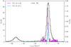 |
Fig. 1 Brightness temperature versus gas velocity. The black histogram corresponds to the H i emission spectrum, magenta to 12CO (j = 1−0), and cyan to 12CO (J = 2−1). The antenna temperature of H i is shown on the left vertical axis and the CO lines on the right vertical axis. The size of each bin is equal to the spectral resolution of each spectrum, i.e., 0.82, 0.16, and 0.32 km s−1 for H i, CO (J = 1−0), and CO (J = 2−1) emission lines, respectively. These spectra were extracted from RA, Dec = 09:33:00, +70:09:00. |
2.2 Optical polarization
We performed polarimetric observations in the optical at the Skinakas Observatory in Crete, Greece1. We used the four-channel imaging robotic polarimeter (RoboPol; King et al. 2014; Ramaprakash et al. 2019). The instrument measures the q and u relative Stokes parameters simultaneously and has a 13.6′ × 13.6′ field of view. In the central part of the field there is a mask (Figs. 2 and 4 in King et al. 2014) that reduces the sky background. The instrumental systematic uncertainty in q and u within the mask is below ~0.1% (Skalidis et al. 2018; Ramaprakash et al. 2019). All the stars were observed within the central mask of the instrument using a Johnson-Cousins R filter. Observations were carried out during four observing runs: 2019 October–November, 2019 May–June, 2019 September–October, and 2020 May - June. The data processing was carried out by an automatic pipeline (King et al. 2014; Panopoulou et al. 2015). We followed the same analysis as in Skalidis et al. (2018) for the calculation of the q and u Stokes parameters and their uncertainties. We computed the degree of polarization as
 (3)
(3)
Uncertainties in q and u are propagated to p assuming Gaussian error distributions for q and u and using Eq. (5) from King et al. (2014). The degree of polarization is always a positive quantity, which is significantly biased toward larger values when the signal-to-noise ratio (S/N) in p is low (Vaillancourt 2006; Plaszczynski et al. 2014). We did not debias the p values since we did not use them in our analysis. Thus, all the p values in the accompanied data table of this paper are biased. The polarization angle was computed as in King et al. (2014),
 (4)
(4)
with the origin of χ being the North Celestial Pole, which follows the international astronomical union (IAU) convention and increases toward the east. Uncertainties in the polarization angles are computed using Eqs. (1) and (2) from Blinov et al. (2021), which are based on Naghizadeh-Khouei & Clarke (1993).
We observed stars up to ~15 magnitude in the R band of the U.S. Naval Observatory-B1.0 catalog (USNO-B1.0; Monet et al. 2003). We extracted the geometric star distances from the Bailer-Jones et al. (2021) catalog, which uses stellar parallaxes from Gaia Data Release 3 (Gaia Collaboration 2021). During each observing night we observed standard stars for instrumental calibration. We used the following standard stars: BD + 28 4211, BD +32 3739, HD 212311 (Schmidt et al. 1992), BD +33 2642 (Skalidis et al. 2018), and HD 154892 (Turnshek et al. 1990). The instrument calibration is performed as in Skalidis et al. (2018).
In Fig. 2, we show our polarization measurements over plotted on the  map of the cloud. Measurements with S/N in fractional polarization higher than 2.5 are shown with colored segments, while measurements with S/N < 2.5 are shown with red circles. The length of each segment and the radius of each circle is proportional to the degree of polarization. In the top-right corner of the figure we show a segment and a circle for scale.
2.3 [C ii] 157.6µm emission line
We observed the 157.6µm emission line of ionized carbon (C+) with the far infrared field-imaging line spectrometer (FIFI-LS; Colditz et al. 2012; Klein et al. 2014; Fischer et al. 2018) onboard the stratospheric observatory for infrared astronomy (SOFIA). The data were obtained in the red channel of FIFI-LS, which covers the 115–2033 µm wavelength range. The field of view consists of a 5 × 5 array of spectral pixels (“spaxels”) with the size of each pixel equal to 12″ × 12″. The spectral resolution at the targeted wavelengths is 1000, which corresponds to a velocity resolution of 270 km s−1. The velocity resolution is much larger compared to typical linewidths of the C+ emission lines (e.g., Goldsmith et al. 2018), and hence the line is spectrally unresolved.
The LOSs are shown in Fig. 2, and their corresponding coordinates are shown in Table 1. Observations were carried out during Observing Cycle 08 as part of the proposal with plan ID 08_0237 (PI: G. V. Panopoulou). The total observing time was 6.5 h, out of which 2.5 h corresponded to on-source time and the rest to off-source time used for calibration. We proposed five different LOSs, but one of them was not used due to the presence of a negative baseline caused by bad weather conditions during the observations. In total we used four out of the five LOSs that were initially proposed. The observations were carried out in “total power mode,” which does not include telescope chopping, but only nodding. We selected regions with low infrared flux (100 µm) to extinction (AV) ratio as nod positions. The off-source (nod position) ratio was selected to be ~100 times lower than the on-source within a chopping angle limit of 45′. Data reduction was performed using the FIFI-LS automatic pipeline. For the SOFIA data processing, we used the SOFIA spectral explorer (SOSPEX2; Fadda & Chambers 2018). We used the highest level pipeline product (level 4), which includes chop subtraction as well as wavelength and flux calibration. We trimmed the frequency axis in order to eliminate frequency bins that were sampled with an exposure time of less than half of the maximum exposure. In practice, this affects only the bins at the edges of the frequency range. We computed the total flux for each LOS within a circular area of 33″ radius in order to increase the S/N. The observed frequency of the [C ii] emission line, 1.9 THz, is highly affected by deep telluric absorption lines. We corrected the fluxes for the telluric transmission using the atmospheric models created by a software tool for computing Earth’s atmoshperic transmission of near- and far- infrared radiation (ATRAN; Lord 1992). Different options exist to parameterize this correction and we followed the most conservative approach, which corrects the fluxes with the transmission value at the reference frequency. Other options resulted in fluxes larger by a factor of ~2. We fitted a third order polynomial to the continuum baseline and subtracted it from the observed fluxes. The continuum-subtracted fluxes are shown in Fig. 3. We fitted Gaussians to the observed spectra. We integrated the Gaussians and divided these values by the beam area (in steradians). The output integral was converted to erg s−1 cm−2 sr−1 and then divided by 6.99 × 10⁻⁶ (Goldsmith et al. 2012) in order to convert to K km s−1. We computed the error on the integrated flux  as follows,
 (5)
(5)
where δν is the frequency bin size and N the number of bins within the integrated interval. The integrated [C ii] intensities can be found in Table 1.
We extracted [C ii] ancillary data from Ingalls et al. (2002) toward the four LOSs shown in Fig. 2. These data have been obtained with the long wavelength spectrometer (LWS) of the Infrared Space Observatory (ISO) and processed by an automatic pipeline. The LWS beam size is 71″’, which corresponds to a beam solid angle Ω = 9.3 × 10⁻⁸ sr. For this data fitting a first order polynomial was sufficient for the background subtraction. In Fig. 4 we show with the colored histograms the baseline-subtracted spectra of the four LOSs. The color of each spectrum corresponds to the LOS shown with a star of the same color in Fig. 2. The blue-shaded region corresponds to the continuum rms. We computed the error in the integrated flux of each Gaussian line, using Eq. (5). In Table 1 we show the integrated fluxes with their corresponding error bars and the LOS coordinates.
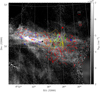 |
Fig. 2 H i column density map of the target cloud. Colored segments correspond to the RoboPol polarization data with S/N ≥ 2.5 that trace the POS magnetic field. Blue and yellow segments correspond to measurements included in the estimation of the magnetic field strength in the atomic and molecular region, respectively. Red segments correspond to measurements with S/N ≥ 2.5 but were not used in the estimation of BPOS (Sect. 3.2). Measurements with S/N < 2.5 are shown with red circles. The radius of each circle corresponds to the observed polarization fraction. A scale segment and circle are shown in the top-right corner. Colored stars correspond to the C+ LOSs from both ISO (orange, black, and yellow) and SOFIA (green, blue, red, and cyan). The size of each star is much larger than the field of view of the instruments. Light green contours correspond to the CO (J = 1−0) integrated intensity at the 3, 5, and 9 K km s−1 levels. The black contours show the CO (J = 2−1) integrated intensity at the 2 and 4 K km s−1 levels. The dashed and solid orange polygons show the CO J = 1−0 and J = 2−1 surveyed regions, respectively. |
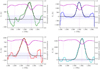 |
Fig. 3 [C ii] emission line spectra of the four LOSs from the SOFIA FIFI-LS spectrometer. The continuum-subtracted fluxes are shown with the histograms. The color of each histogram corresponds to the LOS marked with the same colored star in Fig. 2. Light magenta corresponds to the transmission atmospheric model and the dark magenta histogram to the transmission model convolved with the instrumental spectral resolution. The solid black line corresponds to the Gaussian fit. The blue-shaded region shows the level of the continuum rms. |
Integrated [C ii] intensities.
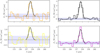 |
Fig. 4 [C ii] emission line spectra, Iλ, versus λ, obtained with ISO (Ingalls et al. 2002). The amplitude of continuum fluctuations is shown with light blue. The solid black lines correspond to the Gaussian fits of the C+ emission line. |
2.4 CO (J = 1−0) emission line
We carried out CO (1−0) observations toward the target cloud with the Purple Mountain Observatory 13.7 m telescope (PMO-13.7 m) from June 3 to 15, 2019 (project code: 19C002). The 3×3 beam sideband separation Superconducting Spectroscopic Array Receiver (Shan et al. 2012) was used as front-end, while a set of 18 fast Fourier transform spectrometers (FFTSs) were used as backend to record signals from both sidebands. Each of the 18 FFTS modules provides 16384 channels, covering an instantaneous bandwidth of 1 GHz. This results in a channel spacing of 61 kHz, that is, 0.16 km s−1 at 115 GHz. The region was mapped in the on-the-fly (OTF) mode (Sun et al. 2018) at a scanning rate of 50″ per second and a dump time of 0.3 s. These observations encompass a total of ~30 observing hours.
The standard chopper-wheel method was used to calibrate the antenna temperature (Ulich & Haas 1976). The antenna temperature,  , is converted into the main beam brightness temperature scale, Tmb, with the relation,
  , where ηeff is the main beam efficiency. The main beam efficiency is 52% at 115 GHz according to the telescope’s status report3. The flux calibration uncertainty is estimated to be roughly 10%. Typical system temperatures were 332–441 K on a
  scale during our observations. The half-power beam width is about 48″ for CO (1−0). The pointing was found to be accurate to within 5”. Data reduction was performed with the GILDAS/CLASS4 software (Pety 2005). A typical 12CO spectrum is shown in Fig. 1.
In Fig. 2, we show with green contours the integrated CO (J = 1−0) flux intensity and the total surveyed area with the large orange polygon. A CO clump is prominent in the right edge of the surveyed area indicating the existence of molecular gas. In addition, we targeted the three LOSs shown with the green, blue and red stars in Fig. 2 in order to overlap with the SOFIA [C ii] data. In Fig. 5, we show the spectra of these three LOSs. The color of each spectrum matches the LOS shown with a star of the same color in Fig. 2. CO was detected only toward the green-star LOS.
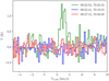 |
Fig. 5 CO (J = 1−0) spectra toward the three LOSs overlapping with our SOFIA data. The horizontal axis is the velocity in the LSR. The labels show the spectrum coordinates. The color of each spectrum corresponds to the LOS shown with colored stars in Fig. 2. |
2.5 CO (J = 2–1) emission line
We used the Heinrich Hertz Submillimeter Telescope5 on Mt. Graham, Arizona, to measure the J = 2−1 transition of CO toward the target cloud. The data were collected on March 1, 3, and 4, 2019. Following Bieging et al. (2014), we used the ALMA Band 6 sideband separating mixers dual polarization receiver to observe the CO (J = 2−1) (230.5 GHz) line. The spectrometers were filter banks with 0.25 MHz bandwidth and 256 filters, providing a spectral resolution of 0.33 km s−1.
The observed region was centered around RA = 9h34m27.63s, Dec = +70° 11′12.2″ (J2000) and was divided into six square subregions of 10’ x 10’ size. Mapping was conducted in OTF mode, by scanning the telescope along lines of constant declination at a scanning rate of 15″ s−1. Spectra were sampled every 0.1 s and later smoothed by 0.4s, corresponding to a telescope shift of 6″ per spectrum. Lines spaced by 10″ in declination were observed in this way. The full width at half maximum (FWHM) of the beam is 32″ for the CO (J = 2−1) observing frequency and is well-sampled with the aforementioned observing strategy. Reference spectra were observed after every other row in good weather and after every row if atmospheric conditions caused high noise levels. Each 10’ × 10’ subregion required 2h of total observing time. Telescope pointing was checked and corrected for every 2h, resulting in pointing errors of less than 5’’ (see Bieging et al. 2014). The intensity was acquired on the scale (Kutner & Ulich 1981) and scaled to main beam brightness temperature by dividing by the measured beam efficiency of 0.776. Measurements of the efficiency were conducted in 2018 by J. Bieging (priv. comm.) following the procedure of Bieging et al. (2010) and Bieging & Peters (2011).
We used standard routines within the CLASS software to remove a linear baseline from each spectrum and map the irregularly sampled data onto a regular grid. During gridding, the data were convolved with a Gaussian kernel whose FWHM is one-third of the beam size, and they were resampled on a regular grid in right ascension and declination with 16’’ grid spacing. The data from all 10’ × 10’ subregions were combined into one map using the fits format within CLASS. The median rms noise of the map is 0.36 K. In Fig. 2, the small solid polygon corresponds to the CO (J = 2−1) surveyed region and the black contours to the CO (J = 2−1) integrated intensity.
3 Connection of the H i–H2 transition to the magnetic field, gas structure, and kinematics
3.1 Characterization of the gas phase properties
The excitation of the [C ii] emission line is due to collisions between C+ and the following collisional partners: hydrogen (atomic and/or molecular) and electrons. The [C ii] emission originates from different layers within a cloud and enables the characterization of its average gas phase properties; emission may originate from a diffuse HI/C+ layer or/and from a cold and dense H2/C+ layer surrounded by the HI/C+ envelope (Velusamy et al. 2010). Our observations do not coincide with star forming regions, and thus we do not expect significant contribution, to the observed [C ii] emission, from dense ionized gas. Ionized gas can still be present, but it is expected to contribute negligibly in this case, ~4% (Pineda et al. 2013). Assuming optical thin conditions, the total [C ii] line intensity can be written as (Goldsmith et al. 2018)
![Mathematical equation: ${I_{\left[ {{{\rm{C}}_{{\rm{II}}}}} \right]}}\left( {{\rm{K}}\,{\rm{km}}\,{{\rm{s}}^{ - 1}}} \right) = N\left( {{{\rm{C}}^{\rm{ + }}}} \right){{6.86 \times {{10}^{ - 6}}n \times {{\rm{e}}^{ - {{91.21} \mathord{\left/{\vphantom {{91.21} T}} \right.\kern-\nulldelimiterspace} T}}}} \over {2.4 \times {{10}^{ - 6}}R_{{\rm{ul:mix}}}^{ - 1} + 4n \times {{\rm{e}}^{ - {{91.21} \mathord{\left/{\vphantom {{91.21} T}} \right.\kern-\nulldelimiterspace} T}}}}},$](/articles/aa/full_html/2022/09/aa42512-21/aa42512-21-eq11.png) (6)
(6)
where N(C+) is the ionized carbon column density and n the total hydrogen number density; Rul;mix is the de-excitation coefficient rate of gas mixed with H i and H2 and it is equal to  , where f(Hi) and f(H2) are the atomic and molecular hydrogen fractional abundances, respectively. The molecular fractional abundance is defined as
 (7)
(7)
The atomic fractional abundance is f(Hi) = 1 − f(H2). The de-excitation rate of H i is  (Barinovs et al. 2005; Goldsmith et al. 2012) and of H2 is [4.9 + 0.22(T/100)] × 10−10n(H2) s−1, valid when 20 ≤ T ≤ 400 (K) with ortho-to-para ratio = 1 (Wiesenfeld & Goldsmith 2014).
Following Langer et al. (2010), we computed the expected I[Cii] as a function of  (Eq. (6)) for different densities (n), and gas temperatures (T) and compared it against the observed values, shown in Table 1. Even though the physical quantities may vary along the LOS, Eq. (6) allows us to consider the mean gas properties (n, f(H2), T) averaged along a LOS. We assumed a [C ii]/H ratio equal to
  (Sofia et al. 2004) and computed the expected N(C+) from the HI/C+ layer as,10
  . We also assumed different f(H2) values in order to estimate
  , and then we computed the corresponding
  of the C+/H2 layer as
  . Overall, the expected I[Cii] versus
  are determined by the following free parameters: n, T and f(H2).
The colored curves in Fig. 6 show the estimated ![Mathematical equation: ${I_{\left[ {{{\rm{C}}_{{\rm{II}}}}} \right]}} - {N_{{{\rm{H}}_{\rm{I}}}}}$](/articles/aa/full_html/2022/09/aa42512-21/aa42512-21-eq22.png) relation for different n, T, and f(H2), as indicated in the legend. Colored points correspond to the observed
relation for different n, T, and f(H2), as indicated in the legend. Colored points correspond to the observed ![Mathematical equation: ${I_{\left[ {{{\rm{C}}_{{\rm{II}}}}} \right]}} - {N_{{{\rm{H}}_{\rm{I}}}}}$](/articles/aa/full_html/2022/09/aa42512-21/aa42512-21-eq23.png) values; the color of each point corresponds to the LOS shown with a star of the same color in Fig. 2. From these points, we detected CO only toward the green and magenta points; this indicates the existence of molecular gas there. We do not have CO observation coverage toward the orange and cyan points.
values; the color of each point corresponds to the LOS shown with a star of the same color in Fig. 2. From these points, we detected CO only toward the green and magenta points; this indicates the existence of molecular gas there. We do not have CO observation coverage toward the orange and cyan points.
The orange, black, and yellow points have a relatively low I[CII]. There is no CO at the black and yellow points, which means that either the gas is atomic or there is a significant amount of H2 but with no corresponding CO emission (CO-dark H2). We can use dust extinction, AV, to trace the total column density toward these LOSs. The total column density is related to the molecular fractional abundance as measured by UV spectroscopy toward background active galactic nuclei (Gillmon et al. 2006; Shull et al. 2021). For these LOSs, we obtained AV from Planck Collaboration Int. XXIX (2016), and then converted to reddening, E(B − V), via RV = AV/E(B − V), where RV = 3.1. For the orange, black, and yellow stars we obtained E(B − V) = 0.25, 0.30, and 0.20 mag, respectively. We then used the relation NH/E(B − V) = 6.07 × 1021 cm−2 mag−1 (Shull et al. 2021) to obtain total column densities for the aforementioned sightlines. The total column density is NH ~ 1.2−1.8 × 1021 cm−2. Sightlines with this range of column densities have at most f(H2) = 0.4 (Fig. 6 of Gillmon et al. 2006). Therefore, in the following we use 0.4 as an upper limit on the fractional molecular abundance for these sightlines.
The relatively low estimated f(H2) values for the aforementioned sightlines indicate that H i gas is more abundant than H2, there. This means that in the [C ii] emission there has a maximum contribution by a HI/C+ layer. If we assume that T = 50 K6, then the yellow and orange points are well represented by the cyan line, which corresponds to T = 50 K, n = 50 cm−3 and f(H2) = 0.1. For the black point, however, a larger n is necessary in order to match with the observed I[C ii] This point is consistent with T = 50 K, n = 100 cm−3 and f(H2) = 0.1. To sum up, gas seems to be mostly atomic toward these LOSs where T = 50 K, f(H2) = 0.1 and n = 50–100 cm−3.
We detected significant 12CO both J = 2−1 and J = 1−0 toward the magenta point. This indicates that there is sufficient amount of molecular gas there; CO emission originates from H2-CO cores formed within H2/C+ envelopes (Langer et al. 2010). Typical H2 temperatures in the Milky Way are 0.7 times lower than their surrounding H i envelopes (Goldsmith et al. 2016). In order to be consistent with the T = 50 K that we assumed for the atomic part of the cloud, we adopted that T = 30 K for the H2 layer there. We obtain that the observed ![Mathematical equation: ${I_{\left[ {{{\rm{C}}_{{\rm{II}}}}} \right]}} - {N_{{{\rm{H}}_{\rm{I}}}}}$](/articles/aa/full_html/2022/09/aa42512-21/aa42512-21-eq24.png) relation at the magenta point can be well represented by n = 200 cm−3, and f(H2) = 0.7, shown with the blue dotted line in Fig. 6.
relation at the magenta point can be well represented by n = 200 cm−3, and f(H2) = 0.7, shown with the blue dotted line in Fig. 6.
At the green, red, cyan, and blue points, I[Cii] is extremely large: ~2 orders of magnitude larger than the other points. These large values can only be obtained if there is a hot (T > 100 K) and dense (n > 100 cm−3) H2/C+ layer. Toward the green point we have detected significant CO (J = 1−0), which means that there is H2 traced by both [C ii] and CO. There, the observed ![Mathematical equation: ${I_{\left[ {{{\rm{C}}_{{\rm{II}}}}} \right]}} - {N_{{{\rm{H}}_{\rm{I}}}}}$](/articles/aa/full_html/2022/09/aa42512-21/aa42512-21-eq25.png) values can be well represented by the red solid line, which corresponds to the following gas properties: T = 400 K, f(H2) = 0.92, and n = 350 cm−3.
values can be well represented by the red solid line, which corresponds to the following gas properties: T = 400 K, f(H2) = 0.92, and n = 350 cm−3.
At the blue, cyan and red points, we did not detect any CO, despite their large [C ii] intensities. This could be related to the fact that these points are close to the edges of the cloud (Fig. 2) and self-shielding is not sufficient to allow for the [C ii]/[CI]/CO transition. The observed large [C ii] intensities can only originate from a hot and dense CO-dark H2 gas layer. This is consistent with previous works, which suggest that CO-dark gas is located at the edges of diffuse clouds (e.g., Langer et al. 2010; Pineda et al. 2013). There, the observed values are consistent with the black solid line, which corresponds to the following conditions: T = 400 K, f(H2) = 0.96 and n = 350 cm−3. We provide estimates of the uncertainty in the derived quantities in Sect. 3.1.1.
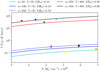 |
Fig. 6 [C ii] integrated intensity versus H i column density. Colored lines show the expected [C ii] intensity assuming that both H i and H2 contribute to the ionization of carbon (see Eq. (6)) with varying temperature, gas density, and molecular fractional abundance. Colored points correspond to the colored-star LOSs shown with the same color in Fig. 2. |
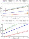 |
Fig. 7 Same as in Fig. 6. Points correspond to the colored-star LOSs shown with the same color in Fig. 2. |
3.1.1 Uncertainties in the estimated gas properties
We used Eq. (6) to constrain the gas properties (n, f(H2), T) based on our [C ii] and  data. However, it is essential to add uncertainties on our estimated values since we use them in the estimation of the magnetic field strength (Sect. 3.2). The large [C ii] intensities of the green, red, blue, and cyan points can be only represented with high n, T, and f(H2) values. In general, the large [C ii] intensities can be fitted only if T > 200 K; otherwise, the exponential in Eq. (6) significantly reduces the expected [C ii] intensity. If we assume T = 300 K, which is typical of CO-dark H2 dominated regions (Langer et al. 2010), then we find that f(H2) ≥ 0.9. In the bottom panel of Fig. 7, the colored solid lines correspond to models with T = 300 K, while the dashed lines to models with T = 400 K. Overall, for these points we find that n = 350–500 cm−3, and f(H2) = 0.91–0.96. Temperatures larger than 400 K are not typical of cold neutral medium (CNM) clouds, and hence were not considered in our analysis; also the molecular de-excitation rate used in Eq. (6) has not been constrained for T > 400 K (Wiesenfeld & Goldsmith 2014).
In the upper panel of Fig. 7, we show the four points with low I[Cii] intensities. The orange, black, and yellow points are dominated by H i gas with f(H2) ≤ 0.4 (Sect. 3.1). If we take this into account the low [Cii] intensities can be only fitted with the red and green solid lines, which correspond to n = 50–100 and T ≈ 50 K. The [Cii] intensity of the magenta point is consistent with the green solid line. However, the significant amount of CO that we detected there indicates that H2 should be more abundant. For the magenta point we found that E(B − V) ≈ 0.55 mag, which is ~2 times greater than the extinction at the black point, and hence f(H2) should be larger at the magenta point. According to Shull et al. (2021), such extinctions are characterized by f(H2) ≥ 0.4. By setting f(H2) = 0.4, and considering that temperature should be lower there (T < 50 K), due to the presence of CO, we find that n ≈ 350 cm−3 (red dashed line). Given the aforementioned constraints, we found that n ≈ 200 cm−3 should be the minimum density toward that point (blue dashed line), and n ≈ 500 cm−3 the maximum density with T ≈ 20 K (green dashed line). We did not consider temperatures lower than 20K because the de-excitation rate of H2 obtained by Wiesenfeld & Goldsmith (2014), and used in Eq. (6), is inaccurate at such low temperatures. To summarize for the orange, black, and yellow points we find that n = 50−100 cm−3 and f(H2) ≤ 0.4, while for the magenta point n = 200−500 and f(H2) ≈ 0.4−0.85 cm−3.
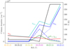 |
Fig. 8 Column densities of different species across the main ridge of the cloud. The color of the horizontal tick labels matches with the colored-star LOSs shown in Fig. 2. The red line corresponds to |


3.1.2 Overview of the gas phases
Here, we summarize the gas phase properties that we inferred for the target cloud from the analysis above. Referring to Fig. 2, as we move across the main ridge of the cloud from the orangestar (RA = 09:48:00) to the magenta-star LOS (RA = 09:30:00), gas transitions from H i to H2; the transition seems to happen between the yellow-star and the magenta-star LOSs, where the CO clump is.
In Fig. 8, we show the adopted H i and H2 column densities at different positions across the long axis of the target cloud. With the red solid line we show  versus RA. The color of the horizontal axis labels corresponds to the LOS marked with a colored-star LOS of the same color in Fig. 2. With the black solid line, we show the assumed gas kinetic temperature, while with the green solid line the observed integrated CO (J = 1−0) intensity (ICO) in K km s−1, multiplied by 1020 for visualization purposes. The H2 column density is indirectly traced by [C ii], and CO and is given by the following equation,
![Mathematical equation: ${N_{{{\rm{H}}_{\rm{2}}}}} = {{f\left( {{{\rm{H}}_{\rm{2}}}} \right)} \over {2\left[ {1 - f\left( {{{\rm{H}}_{\rm{2}}}} \right)} \right]}}{N_{{{\rm{H}}_{\rm{I}}}}} + {X_{{\rm{CO}}}}{I_{{\rm{CO}}}}.$](/articles/aa/full_html/2022/09/aa42512-21/aa42512-21-eq30.png) (8)
(8)
The first term corresponds to CO-dark H2 and is inferred by the f(H2) values that we obtained from the [C ii] observations, while the second term corresponds to CO-bright H2. XCO is the conversion factor between H2 and CO, and has a typical value in our Galaxy equal to XCO = 2 × 1020 cm−2 K km s−1 (Bolatto et al. 2013), although variations can be significant in individual cases (e.g., Barriault et al. 2011). In the same figure, we also show the column density of CO-dark H2 with the blue dotted line, and of CO-bright H2 with the blue dash-dotted line.
There are three major uncertainties introduced in our estimated  values (Eq. 8). Firstly, the derived f(H2) values are degenerate with n and T. Secondly, XCO can vary significantly throughout our Galaxy (e.g., Barriault et al. 2011), and hence the mean XCO that we adopted may not be representative of the target cloud. Thirdly, there is H2 gas traced only by [Ci] (Pineda et al. 2017); the contribution of this layer was neglected in the estimated column densities since we do not have [Ci] observations for this cloud. We cannot overcome these problems with the existing data set, and for this reason we note that the values shown in Fig. 8 offer a qualitative characterization of the gas phase properties of this cloud.
Kalberla et al. (2020) created a full-sky column density map of the CO-dark H2 gas. They estimated the total column densities with data from the HI4PI survey (HI4PI Collaboration 2016) and the extinction map of Schlegel et al. (1998). Our adopted picture shown in Fig. 8 is consistent with their map; the CO-dark H2 column densities increase toward the green-star and blue-star LOSs. Since the data from this map are similar to our properties for the  , it gives us confidence that Fig. 8 accurately represents the atomic-to-molecular gas transition of this cloud. However, a direct comparison between our inferred values and their map may not be meaningful due to following main reasons: 1) There is a significant difference in the angular resolution of the Kalberla et al. (2020) map (11′) and our data (0.55′ and 1.18′ for the SOFIA and the ISO data, respectively), 2) Their map is based on the assumption that the E(B – V)/NH ratio is constant throughout our Galaxy, and 3) f(H2), which is inserted in our
  computation, is degenerate with n and T.
3.2 Magnetic field strength
We employed the method of Skalidis & Tassis (2021; ST) to estimate the strength of the plane-of-the-sky (POS) magnetic field component, BPOS. In contrast to the widely applied method of Davis (1951) and Chandrasekhar & Fermi (1953; DCF), which assumes that the dispersion of polarization angles (δχ) is induced by incompressible waves, this method assumes that compressible fluctuations are the dominant; ST was found to give better magnetic field strength estimates than DCF when tested against MHD numerical simulations that do not include self-gravity, even for super-Alfvénic models with MA = 2.0 (Skalidis et al. 2021). The POS magnetic field strength can be estimated as
 (9)
(9)
where p is the gas volume density and σv,turb the gas turbulent velocity. This equation is applicable when δχ ≪ 1 rads.
3.2.1 Polarization angle dispersion estimation
It is evident from Fig. 2 that the mean magnetic field orientation is not uniform within the cloud, which complicates the computation of δχ. At the orange-star LOS, the magnetic field follows the  structure of the cloud, while between the black- and yellow-star LOSs a transition happens; the mean field orientation tends to be perpendicular to the
  structure of the cloud; this is discussed in more detail in Sect. 4. This change in the mean field orientation induces extra spread in the distribution of polarization angles, which is not related to MHD waves.
In order to accurately constrain the MHD wave-induced dispersion (intrinsic dispersion, δχintr), we removed measurements located between the black-star and yellow-star LOS in Fig. 2; this is the transition zone where the mean magnetic field orientation changes. Then, we classified two distinct subregions within the cloud. The first region corresponds to measurements located between RA = 09:53:00 and RA = 09:39:22 (black-star LOS in Fig. 2). The mean magnetic field orientation of these measurements is parallel to the  structure of the cloud, and gas is mostly atomic there. Hereafter, we refer to this region as “atomic.” The second classified region includes all measurements between the yellow-star and blue-star LOSs (Fig. 2), from RA = 09:34:39 to RA = 09:22:41. The mean magnetic field orientation of these measurements tends to be perpendicular to the
  structure of the cloud, and gas is mostly molecular there. We refer to this region as “molecular”.
In both regions, we applied three statistical criteria in order to minimize the various sources of uncertainty that bias δχ toward larger values. Firstly, we considered only measurements with S/N ≥ 2.5. Secondly, we considered only polarization measurements of stars located behind the target cloud, but not very far away to be affected by the IVC cloud; the target cloud is located at 300 pc (Appendix A), while the IVC cloud at 1kpc (Tritsis et al. 2019). In this step, we included stars with distances 300 ≤ d ≤ 1000 pc. This guarantees that the polarization measurements are not affected by the IVC cloud, which, despite its weaker H i emission (Fig. 1), may significantly contribute in the total polarization, as shown by Panopoulou et al. (2019b). Thirdly, we discarded stars with polarization angles offset by more than 60° from the mean orientation. This ensures that our analysis is not affected by potentially intrinsically polarized stars. These measurements do not probe the morphology of the ISM magnetic field and they are outliers in the polarization angle or degree of polarization distributions. In total, we found only two outliers in the polarization angle distribution of the atomic region. The measurements used for the BPOS estimation in the atomic region are shown as blue segments in Fig. 2, while measurements included BPOS estimation of the molecular region are shown in yellow. Measurements with S/N ≥ 2.5 that did not meet the aforementioned selection criteria and were not included in the BPOS estimation are shown in red.
The distribution of polarization angles (χ) is shown in Fig. 9. The upper left panel corresponds to the distribution of χ for the atomic region, while the upper right panel shows their corresponding observational uncertainties (σχ). The two lower panels show the same quantities for the molecular region. We performed an optimal binning to these distributions following Knuth’s rule Bayesian approach as implemented in astropy. We fitted Gaussian profiles in the χ distributions as shown with the cyan solid lines. In the atomic region, the spread of the fit is equal to 18°, which is very close to the raw spread (20°) of the distribution. In the molecular region, both the spread of the fit and the raw spread of the distribution are approximately equal to 15°. Observational uncertainties tend to bias the spread of the χ distribution to larger values. For this reason, we corrected for the observational uncertainties following Crutcher et al. (2004) and Panopoulou et al. (2016) as
 (10)
(10)
where  is the mean observational uncertainty. The mean uncertainty in the atomic region is
  , while in the molecular region it is
  . For the atomic and molecular regions, the derived intrinsic spreads corrected for the observational uncertainties are δχint = 16.8° and 14.4°, respectively, as shown in Table 2.
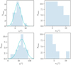 |
Fig. 9 Distribution of polarization angles and their observatinal uncertianties. Top-left panel: dispersion of polarization angles for the atomic region. The solid cyan profile corresponds to the fitted Gaussian. The mean (µ), standard deviation (σ), and amplitude (α) of the fit are (µ, σ, α) = (63°, 18°, 9). Top-right panel: polarization angle error distribution. Bottom panels: same as for the upper panels, but for the molecular region. The free parameters of the fitted Gaussian are (µ, σ, α) = (12°, 15°, 8). |
3.2.2 Turbulent gas velocity and density estimation
Gas turbulent velocities, σu,turb, were computed from the H i and CO emission lines. H i spectra probe the atomic gas layers kinematics, while CO probes the molecular layers. We computed the average spectra in both regions and fitted their profiles with Gaussians. We subtracted the thermal broadening via a quadrature subtraction,
 (11)
(11)
where σv,turb is the standard deviation of the Gaussian fitting and i refers to the mass of the emitting species, which is either H i or 12CO. Following our estimates in Sect. 3.1, the mean gas temperature in the atomic region is T = 50 K (orange and black star in Fig. 6), while in the molecular region it is T ≈ 300 K (magenta, green, blue and cyan stars in Fig. 6) for the CO-dark layer, while for the CO-bright layer we assumed that T = 15 K. Overall, our calculations are not very sensitive to temperature variations. In Table 2 we show the turbulent velocity spreads in km s−1 for both regions.
The emission of chemical tracers originates from local regions (layers) within a cloud, and hence it traces the local and not the average cloud kinematics. On the other hand, dust polarization is averaged along every gas layer in the cloud, and as a result it represents the average magnetic field fluctuations of the cloud. Thus, there is an inconsistency between the two observables (polarization and velocity broadening) since they do not trace the same regions of the cloud. In the atomic region the aforementioned problem is not so prominent, since there is a dominant H i gas layer (Sect. 3.1). In that case, the spread derived from the H i emission line fitting should accurately represent the average gas kinematics. In the molecular region, however, there is both atomic and molecular gas, with the latter being the most abundant. We computed the weighted rms turbulent velocity in the molecular region as
![Mathematical equation: ${\sigma _{v,{\rm{turb}}}}{\left\{ {{f_{{\rm{HI}}}}{{\left[ {{\sigma _{{\rm{turb,}}{{\rm{H}}_{\rm{I}}}}}} \right]}^2} + f_{{{\rm{H}}_{\rm{2}}}}^{{\rm{dark}}}{{\left[ {\sigma _{{\rm{turb,}}{{\rm{H}}_{\rm{2}}}}^{{\rm{dark}}}} \right]}^2} + f_{{{\rm{H}}_{\rm{2}}}}^{{\rm{bright}}}{{\left[ {\sigma _{{\rm{turb,}}{{\rm{H}}_{\rm{2}}}}^{{\rm{bright}}}} \right]}^2}} \right\}^{{1 \mathord{\left/{\vphantom {1 2}} \right.\kern-\nulldelimiterspace} 2}}},$](/articles/aa/full_html/2022/09/aa42512-21/aa42512-21-eq44.png) (12)
(12)
where the first term corresponds to the kinematics contribution from the H i layer, the second to a CO-dark H2 layer, and the third term to a CO-bright H2 layer; fH i,  , and
, and  are the fractional abundances of the H i, CO-dark H2, and CO-bright H2 layers, respectively, which are defined as
 (13)
(13)
 (14)
(14)
 (15)
(15)
The motivation behind Eq. (12) is that the molecular region is characterized by three different gas layers. Equation (12) can be verified by computing the mean spread of three Gaussians centered at the same velocity with different spreads and with amplitudes that are proportional to the relative abundance of each species.
In Fig. 8, we show our inferred column densities of each layer. Based on these estimates we computed the mean abundance of each layer, which are fHI ≈ 0.07,  ≈ 0.66, and
  ≈ 0.27;
  is the H i broadening, while
  the CO (J = 1−0) broadening. In Eq. (12) the only parameter that is not observationally constrained is
  . For this reason, we assumed similarly to past works (e.g., Panopoulou et al. 2016) that the CO broadening is an accurate proxy for the averaged H2 kinematics, which means that both the CO-darkand CO-bright H2 layers share similarkinematics properties, hence
  . We derived that the mean turbulent broadening is 1.15 km s−1 in the molecular region.
We averaged the density over all layers in the molecular region as
 (16)
(16)
where mp is the proton mass,  is the mean atomic mass, and
  is the mean molecular weight,
  the mean volume density of the H i layer,
  the mean volume density of the CO-dark H2 layer, and
  the mean volume density of the CO-bright H2 layer. From the analysis in Sect. 3.1, we find that the average density and molecular fractional abundance are f(H2) ≈ 0.86 and n ≈ 300 cm−3, respectively; these two quantities, however, refer only to the H i and CO-dark H2 layers, which are probed by the [C ii] emission line data. Using these values, we computed
  and
and  as,
as,  = n × [1 − f(H2)] = 42 cm−3, and
  = n × f(H2) = 258 cm−3.
In order to estimate  we need to make some assumptions regarding the 3D shape of the CO clump. For dynamically important magnetic fields, like ours (Sect. 3.2.3), oblate shapes are favored; this has been verified observationally by Tassis et al. (2009). The size of the major axis of the CO clump on the sky is ~0.4°, which corresponds to 2.0 pc, while its minor axis is ~0.1° and corresponds to 0.5 pc. Given an oblate 3D shape, it is reasonable to assume that the depth of the H2-CO layer is closer to the size of its major axis than its minor axis. For this reason, we assumed that the LOS dimension of the core is 1.5 pc. For the molecular region, our estimated mean CO-bright
  column density is 8.6 × 1020 cm−2, which yields
  ≈ 400 cm−3. Then the estimated weighted mean number density in the molecular region is 〈n〉 ≈ 290 cm−3. In the atomic region there is negligible H2, hence f(H2) ≈ 0,
  , and
, and  . Density uncertainties are propagated to the final BPOS estimates as shown in Table 2.
Magnetic field strength and Alfvénic Mach number estimation.
3.2.3 POS and total magnetic field strength
There are three major uncertainties that affect the BPOS estimation: variations in temperature, molecular fractional abundance, and density within the two regions (atomic and molecular), with the gas density being the dominant source of uncertainty. In the atomic region the number density inferred from our [C ii] data varies from 50 to 100 cm−3 and in the molecular region from 200 to 500 cm−3 ( Sect. 3.1). We estimated the limits on BPOS based on the full range of density values found for each region. However, for the molecular region, f(H2) is also an important source of uncertainty, since it affects the estimated turbulent velocity in Eq. (12). Thus, for the molecular region we varied both n and f(H2) in the range that we established from our [C ii] models in Sect. 3.1.1. The lower limit on BPOS is found for f(H2) = 1.0 and  cm−3 and the upper limit is found for f(H2) = 0.4,
  cm−3, and
  cm−3. In Table 2, we show the estimated BPOS with corresponding limits for both regions; the POS magnetic field strength is consistent within uncertainties between the two regions.
For the current cloud, there are archival H i Zeeman data (Myers et al. 1995) tracing the LOS magnetic field strength (BLOS). We combined the BLOS measurements from this data set with our BPOS estimated values and derived the total magnetic field strength of the cloud, Btot. We computed the mean BLOS of both the atomic and molecular regions; the minimum and maximum BLOS values of each region were used as lower and upper limits, respectively. For both regions, it is true that BLOS < BPOS, which indicates that the magnetic field of the cloud is mostly in the POS. We computed the 34% and 83% percentiles of their BLOS distribution in every region and used these upper (and lower) limits with the corresponding limits from our BPOS estimates to derive the upper (and lower) limits of Btot. We find that the Btot estimated values between the two regions are consistent within our uncertainties. We note, however, that in the molecular region BLOS may not be representative of the total LOS magnetic field component. The existing Zeeman data trace only the H i layer and not the bulk of the gas, which is mostly molecular there (Sect. 3.1). Thus, in the molecular region Btot should be treated as a lower limit of the total magnetic field strength.
3.2.4 Estimating the Alfvén Mach number
In addition, we estimated the Alfvénic Mach number MA of the cloud. According to ST the projected Alfvén Mach number is  . We find that
  in the atomic region, while
  in the molecular region. The total (3D) Alfvén Mach number will be
  , where C is a constant. For isotropic turbulence
  . However, recent ideal-MHD numerical simulations suggest that magnetic fluctuations become fully isotropic when MA ≥ 10 (Beattie et al. 2020). According to their results (Fig. 6), parallel magnetic fluctuations are ~0.5–0.6 times smaller than perpendicular when 0.5 ≤ MA ≤ 2. If we also consider that the dispersion of polarization angles probe perpendicular magnetic field fluctuations (e.g., Skalidis et al. 2021), we derive
  ; this is a more reasonable value than simply assuming that turbulence is isotropic and
  .
.
Then we find that MA ≈ 1.2 and MA ≈ 1.1 for the atomic and molecular region, respectively. For both regions MA ~ 1, which indicates that turbulence is trans-Alfvénic in this cloud, which means that the magnetic field is dynamically important. It is not straightforward to impose uncertainties on this estimate, and hence MA could be slightly below or above one. This uncertainty, however, cannot affect our conclusion about the relative importance of the magnetic field in the cloud dynamics; in order to consider the magnetic field as dynamically unimportant (or equally that turbulence is purely hydro), MA should be larger than two (Beattie et al. 2020). Even if we set  , which would be an upper limit, the estimated MA is less than 1.4 for both regions. Our results are consistent with Planck Collaboration Int. XXXII (2016), who found that turbulence in the diffuse ISM is sub- or trans-Alfvénic.
3.3 Is the magnetic field morphology correlated with the H i velocity gradients?
Our estimates indicate that turbulence is trans-Alfvénic in the target cloud (Sect. 3.2). This means that the magnetic field should play an important role in the dynamics of the cloud. Theoretical scenarios suggest that, for dynamically important fields, the morphology of the field lines is correlated with the gas velocity gradients (e.g., González-Casanova & Lazarian 2017; Girichidis 2021). There are two favored topological states toward that the magnetic field tends to: the orientation of the field is either perpendicular or parallel to the orientation of the gas velocity gradient. According to GonzálezGonzalez-Casanova & Lazarian (2017) the orthogonality between the magnetic field and the velocity gradient field is due to the strong Alfvénic motions that develop within a cloud. The same configuration can be achieved in clouds formed in the boundaries of bubbles when gas is expanding perpendicular to the background ISM magnetic field (e.g., Girichidis 2021). When gravity takes over, velocity gradients tend to become parallel to the magnetic field (e.g., Lazarian & Yuen 2018; Hu et al. 2020; Girichidis 2021). We tested these scenarios by exploring the correlation between the magnetic field morphology and the H i velocity gradients in the target cloud.
The H i LOS velocity component, Vc(α, δ), is the first moment of the brightness temperature map, Tb(α, δ), and we computed it as in Miville-Deschênes et al. (2003b),
 (17)
(17)
where the summation is performed within the velocity range relevant to the target cloud, which is [−22.1, 20.8] km s−1 (Fig. 1). We computed the Vc gradient field using second order central differences for every pixel. We smoothed the Vc map with a Gaussian kernel with standard deviation equal to 5.8′ in order to reduce the noise in the map. We computed the velocity gradient orientations7 as
 (18)
(18)
and the amplitudes as
 (19)
(19)
Fluctuations in Tb can lead to ∣∇Vc∣ ≠ 0, even in the absence of a gradient; this can happen when there are multiple gas components with varying intensities. As we show in Appendix D this does not seem to be the case for the target cloud, where there is a dominant H i component. Thus, the H i gradients computed with the equations above accurately represent the projected H i kinematics of the target cloud.
In Fig. 10, we show the velocity gradient field with red segments overplotted on the  map of the cloud; cyan segments correspond to our polarization measurements. In the atomic part of the cloud toward the orange-star LOS, velocity gradient orientations tend to be perpendicular to the magnetic field orientation. This behavior seems to hold in the majority of the cloud, as for example close to the cyan-star and yellow-star LOSs. But, toward the CO clump and close to the magenta-star LOS, velocity gradients tend to be parallel to the magnetic field. This alignment happens locally above the CO clump. Simulations suggest that velocity gradients are parallel to the local magnetic field orientation when gas is undergoing gravitational collapse (e.g., Lazarian & Yuen 2018; Hu et al. 2020). Recently, Girichidis (2021) found that gravity takes over at n ~ 400 cm−3, which is consistent with our inferred density for the CO-bright region of the target cloud derived by assuming an oblate triaxial 3D shape for the CO clump. Thus, it is probable that the observed H i velocity gradient alignment with the local magnetic field morphology above the CO clump is due to gas that accretes onto the clump.
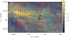 |
Fig. 10 Velocity gradients overplotted on the |

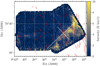 |
Fig. 11 CO (J = 1−0) integrated intensity. White lines mark the major and minor axis of the CO clump. Red segments show the polarization measurements as in Fig. 2. The long red line at the center of the core corresponds to the mean magnetic field orientation. |
3.4 Does the magnetic field affect the CO clump shape?
The magnetic field is considered to affect the accumulation of gas (e.g., Mouschovias 1978; Heitsch et al. 2009). When the field is dynamically important, it can support a cloud against its own self-gravity; magnetic forces are exerted perpendicular to the field lines, and hence the magnetic field supports a cloud against its self-contraction perpendicular to the field lines. As a result, gas preferentially accumulates parallel to field lines and the molecular clump is flattened, with its small axis parallel to the mean magnetic field orientation. For dynamically unimportant magnetic fields, no correlation between the mean field orientation and the clump shape is expected. For this reason, we explored if the shape of the CO clump is connected with the magnetic field as predicted by theoretical scenarios.
Following Tassis et al. (2009), we computed the center and the shape of the CO clump using the first and second moments of the CO (J = 1−0) integrated intensity map, ICO(x, y), shown in Fig. 11. We found that the aspect ratio between the two principal axis is 0.4, which implies that the structure is slightly flattened; an aspect ratio equal to 1 means that the clump is circular. Our polarization measurements are shown with the red segments in Fig. 11. The figure shows the mean polarization angle of the measurements close to the CO clump, that is, the region defined by the following boundaries: 09:28:00 ≤ RA ≤ 09:36:00 and +70:00:00 ≤ Dec ≤ 70:40:00.
The mean magnetic field orientation is closer to the minor principal axis of the clump than the major axis, with a 24° offset. Although the alignment of the mean field orientation with the minor clump axis is not exact, our observations indicate that the magnetic field is likely responsible for the asymmetric shape of CO clump. This, in combination with the alignment that we found between the H i gradients with the magnetic field above the clump, suggests that the CO clump could be self-gravitating.
Our results are in line with Tassis et al. (2009), who find that the mean magnetic field orientation is ~20° offset from the minor axis of asymmetric molecular cores. These authors targeted cores with densities 103−104 cm−3, which is significantly larger than our inferred densities (~400 cm−3 for the CO-bright clump). Our inferred alignment is slightly weaker than the average alignment found by Tassis et al. (2009). A possible explanation is that the gas volume density of our cloud is one (or in some cases two) orders of magnitude less than the core densities studied by Tassis et al. (2009). This implies that self-gravity may have a weaker role in the dynamics of our clump than in the dense cores of their sample.
Finally, we note that the CO survey of Pound & Goodman (1997), toward the same cloud, showed that this clump is slightly extended further from the boundaries of our map, toward RA = 09:28:00 and Dec = +70:30:00. However, the difference of the integrated intensity maps between the two data sets is not significant and does not affect the qualitative conclusions on the clump shape. In fact, using the data from Pound & Goodman (1997) we found that the offset between the minor axis of the clump and the mean magnetic field orientation is reduced by 6°; we refer to Fig. 1 of Miville-Deschênes et al. (2002) for a visual comparison of our inferred clump shape with the data from Pound & Goodman (1997).
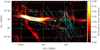 |
Fig. 12 Our starlight polarization measurements (cyan segments) overplotted on the RHT output image. The colorbar shows the normalized intensity measured from the RHT. Stars and CO contours have the same meanings as in Fig. 2. |
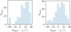 |
Fig. 13 Distribution of relative orientations. Left panel: distribution of the difference between the orientation of the |

4 Is the magnetic field morphology correlated with the H i structure of the cloud?
Diffuse H i elongated clouds were found to be statistically aligned with the Galactic magnetic field, as probed by dust polarization (Clark et al. 2014, 2015; Kalberla et al. 2016). Our polarization data (Fig. 2) follow the main H i structure in the left (atomic) part of the cloud, RA > 09:36:00, while in the right (molecular) part, RA ≤ 09:36:00, they tend to be perpendicular to the cloud axis.
We employed the rolling Hough transform (RHT; Clark et al. 2014) in order to quantify the relative alignment between our polarization orientations and the H i structure. The input of this algorithm is the column density map of Fig. 2. The algorithm uses a circular kernel of radius Dw and smooths the image. A kernel with radius Dk scans the image and measures the probability of each pixel being part of a linear structure along different orientations (θ). Orientation angles, θ, with a probability larger than a given threshold, Z, are identified as linear structures. We set the free parameters of the RHT algorithm close to the authors recommended values, Dw = 95′, Dk = 30′ and Z = 70%. The output of the RHT is shown in Fig. 12.
The color map shows the linearity intensity normalized in the range [0, 1]. The algorithm has detected the main structure of the cloud at RA ≤ 09:40:00, which then splits into two branches of lower linearity at RA ~ 09:40:00 close to the black-star LOS. Cyan segments correspond to our polarization data, contours to the CO integrated intensity, and colored stars to the LOSs where [C ii] are available, as in Fig. 2. We quantified the relative difference between the polarization angles and the H i cloud orientation. We computed the orientation angle of the H i structure as suggested by Clark et al. (2014), within circular regions of radius equal to 15’ and centered at the position of each polarization measurement. The H i orientation angles, or RHT angle, are denoted as θRHT and the polarization angles as χ We computed the difference between θRHT and χ restricted in the range [−90°, 90°]. In Fig. 13, we show the distribution of differences between the two quantities. The circular mean of the distribution is 43°, which in striking contrast to Clark et al. (2014), shows that the relative alignment of the H i structure with our optical polarization orientation is weak; the loss of alignment happens close to the CO clump. Thus, the H i structure of the cloud is not a good proxy of the magnetic field orientation in the molecular region of the target cloud.
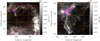 |
Fig. 14 Magnetic field morphology overplotted on the Planck-based NH map of the NCPL. Left panel: dust emission polarization rotated by 90°, shown by red segments. The length of each segment is proportional to the polarized intensity. Magenta segments correspond to our polarization measurements; all segments have a fixed size for visualization purposes. There is an offset in the magnetic field orientation as traced by optical and submillimeter polarization due to the large beam difference between the two observables. Colored stars correspond to the target C+ LOSs, as shown in Fig. 2. Right panel: zoomed-in view of the region toward the target cloud. The solid cyan segment shows the Hα canal found by McCullough & Benjamin (2001). |
4.1 What caused the magnetic field turn in the target cloud?
In the molecular region of the target cloud, the magnetic field orientation turns and does not follow the H i structure. This turn could be caused by the self-gravity of the CO clump. However, the onset of the magnetic field turn happens at RA = 09:40:00, close to the black-star LOS in Fig. 12. This is ~0.8° away from the center of the CO clump and corresponds to an actual distance of ~4 pc. This offset distance is significant, and hence it seems unlikely that the self-gravity of the dense CO-bright core could have significantly distorted the magnetic field lines of the cloud at such a large distance from it. Thus, we examined other scenarios that could potentially explain the origin of this turn in the magnetic field morphology.
The target cloud is located close to the Ursa Major arc, which is a 30 degree long structure observed in ultraviolet wavelengths. As was suggested by the authors who discovered this arc (Bracco et al. 2020), it is plausible that it was formed by a radiative shock. If that is the case, then the magnetic field morphology of the target cloud may have been distorted by a large-scale explosion. Indeed, the cloud is at the edges of the so-called NCPL (Heiles 1989), which is considered to be an expanding cylinder or sphere (Meyerdierks et al. 1991). Thus, the NCPL explosion could have caused the observed turn of the cloud magnetic field morphology with respect to the  axis. We explored if simple energetics arguments support this idea. For, if the magnetic field were sufficiently strong, it could prevent gas from expanding and the magnetic field lines would be relatively straight. In the opposite case, the expanding gas could drag the field lines, and hence create large-scale magnetic field distortions.
The NCPL is expanding with a velocity uexp ~ 20 km s−1 (Meyerdierks et al. 1991). If we assume that the density of the expanding gas in the boundaries of the bubble is ~100 cm−3 8, then the kinetic energy density of the expanding gas is 3.2 x 10⁻¹⁰ gr cm−1 s2. The magnetic field energy density, adopting from Sect. 3.2 that ∣Btot∣ ~ 30 µG, is 1.6 × 10⁻¹¹ gr cm−1 s2; the ratio of the kinetic over the magnetic energy density is ~ 10. Thus, the NCPL expansion has enough energy to distort the magnetic field morphology of the cloud. Since the observed magnetic field turn of the cloud is probably related to the NCPL expansion, we explored if the magnetic field morphology of the NCPL is consistent with an expanding bubble or cylinder.
In the left panel of Fig. 14, we show the NH map of the NCPL. For the construction of the NH map we used the extinction map from Planck Collaboration Int. XXIX (2016), AV, and the conversion factor NH/E(B − V) = 6 × 1021 cm−2 mag−1 (Kalberla et al. 2020), where AV/E(B − V) = 3.1. A characteristic hole is prominent at l, b ~ (135°, 35°) possibly due to the expansion of the NCPL. Our target cloud is located at the edges of the loop at coordinates, l, b = 142°, 39°. In the right panel of Fig. 14, we show a zoomed-in region toward the target cloud; magenta segments correspond to our polarization9 measurements.
We probed the magnetic field morphology of the NCPL using the 353 GHz dust emission polarization data from the Planck satellite (Planck Collaboration XII 2020). We smoothed the Stokes parameter maps at a resolution of 1° in order to increase the S/N (as described in Skalidis & Pelgrims 2019). In the left panel of Fig. 14, we show the Planck polarization rotated by 90° in order to probe the POS magnetic field orientation, with the length of each segment proportional to the polarized intensity, which is
 (20)
(20)
where Is, Qs, and Us are the Stokes parameters measured by Planck. The polarization orientation is
 (21)
(21)
measured in the Galactic reference frame, and following the IAU convention angles increase counterclockwise.
The magnetic field lines are squeezed in the right edge of the NCPL l, b ~ 126°, 33°, while in the left part l, b ~ 142°, 33° they are well ordered and parallel to each other; this indicates that NCPL expanded asymmetrically. In the left part, 140° ≤ l ≤ 145° and 35° ≤ b ≤ 40°, gas seems to have escaped from the bubble without distorting the magnetic field lines, while in the right part, the swept-up gas could have collided with the background ISM and created regions with enhanced column density, such as those at l, b ~ 126°, 30°. The background ISM magnetic field is almost parallel to the Galactic Longitude axis at 136° ≤ l ≤ 145° and 38° ≤ b ≤ 40°. Overall the magnetic field morphology is consistent with an expanding bubble or cylinder; simulated morphologies from Krumholz et al. (2007) and Ntormousi et al. (2017) can be used for a visual comparison. The magnetic field morphology of our target cloud exhibits a turn with respect to the background field of this area (right panel in Fig. 14): it forms an angle with the latter at b > 39° and becomes parallel to the ambient field at b < 39°. Thus, it is likely that the NCPL expansion is responsible for the observed turn of the magnetic field orientation with respect to the  axis in the molecular region of the target cloud, Fig. 2.
There is also a possibility that a smaller-scale expansion, other than the NCPL, affected the magnetic field morphology of the cloud. In the right panel of Fig. 14 we see that the target cloud is close to another cloud located at l, b ~ 142°, 34.5°. This cloud also has a significant amount of CO (Pound & Goodman 1997), and its magnetic field morphology (red segments) also turns with respect to the ISM background magnetic field. The NH morphology of this cloud combined with our target cloud’s structure creates a bow-like structure, assuming that the center is at ~138°, 37.5°, which is typical of clouds located at the boundaries of expanding bubbles (Inoue & Inutsuka 2008, 2009). One more piece of evidence that indicates that the two clouds could be at the boundaries of a bubble unrelated to the NCPL is that McCullough & Benjamin (2001) found a narrow and filamentary Hα canal close to our target cloud, shown in the right panel of Fig. 14. From the various models they explored, they concluded that this canal was most probably formed due to the trail of a star or another compact object that moves through the ISM. This canal points toward our target cloud and could have been formed by an object kicked by an explosion: the same explosion that swept up the gas and formed our target cloud at the boundaries of this bubble. The magnetic field lines (red segments) follow the bow-like shape of the two clouds, and they seem to form a bottleneck at l, b ~ 144°, 38°, where they get squeezed and turned, eventually connecting with the background ISM field. Thus, it is plausible that expanding gas, which is not related to the NCPL, dragged the magnetic field lines of our target cloud and created the observed offset between the  axis of the cloud and its magnetic field orientation in the molecular region.
4.2 Correlation of the magnetic field morphology with total column density
We applied the RHT algorithm to the NH map of our target cloud shown in Fig. 14 with the following parameters Dw = 41′, Dk = 25′ and Z = 70%. The output of the RHT analysis is shown in Fig. 15 with our polarization segments overplotted in cyan. In the atomic region of the cloud, defined between the orange and black stars, the NH-RHT morphology tends to be parallel to the magnetic field orientation. Since atomic gas is more abundant there, the  map probes almost the total column density (NH), and hence both the RHT-
 (Fig. 12) and RHT-NH (Fig. 15) maps are consistent there. In the molecular region, there is a major difference between the RHT structures of
  and NH when compared with the local magnetic field orientation.
In the molecular region of the cloud (between the yellow and black stars), the RHT-NH structure splits into two branches; the first branch is toward the CO clump (green contours), where the RHT structure tends to be perpendicular to the magnetic field orientation, and the second branch is toward the cyan point, where the RHT structure tends to align with the magnetic field. On the other hand, in the molecular region, the RHT- map splits into two branches that are both perpendicular to the mean magnetic field orientation. The distribution of the difference between the RHT angles and our polarization data for the NH map is shown in the right panel of Fig. 13; the mean of the distribution is 20°, which implies that the total column density of the cloud tends to be parallel to the local magnetic field orientation. Although, the alignment between the POS magnetic field orientation and the NH shape of the cloud is not perfect (20° offset), it is stronger than the alignment between the magnetic field morphology and the
  shape (43° offset).
5 Does the magnetic field affect molecule formation in the NCPL?
The magnetic field is considered to play an important role in the formation of H2 in expanding bubbles (e.g., Walch et al. 2015; Girichidis et al. 2016; Girichidis 2021). Gas that is expanding parallel to the magnetic field, can free stream and finally escape from the bubble. This leads to the formation of low column density regions (tunnels). On the other hand, gas that is expanding perpendicular to the magnetic field compresses the field lines and induces a magnetic pressure gradient, which is exerted against the gas expansion. The magnetic field prevents gas from escaping and thus forms regions with enhanced column densities, which define the boundaries of the bubble. These regions are candidates for hosting molecular clumps, if self-shielding is sufficient to prevent the H2 photo-destruction. Thus, one would expect that H2 is preferentially formed near the bubble boundary regions, where the relative orientation between the magnetic field and the H i velocity gradients is perpendicular. When gas accumulation becomes important, self-gravity takes over and then H i velocity gradients align with the magnetic field (e.g., Hu et al. 2020). Although, it has been suggested that the magnetic field could determine the location of molecular sites in expanding structures (e.g., Dawson et al. 2011), to our knowledge no systematic observational study has ever been done regarding this topic. For this reason, we used the correlation between the magnetic field and the H i velocity gradients in order to explore if the relative orientation between the two is connected to the molecular gas in the wider NCPL region.
We used data from the HI4PI all-sky survey (HI4PI Collaboration 2016) in order to study the H i kinematics of the NCPL; the higher resolution DHIGLS survey (Blagrave et al. 2017) does not cover the full region of the NCPL. The resolution of the HI4PI data is 10.8′. We also employed the full-sky  map of Kalberla et al. (2020) in order to infer the NCPL H2 sites and the full-sky map of total hydrogen column density, NH, provided by the same authors. These maps allowed us to probe the molecular fractional abundance toward the NCPL.
The observed H i spectra include contribution from multiple sources that may be spatially distinct, or from clouds at different ISM phases, such as the warm neutral medium (WNM) and the CNM. In order to study the kinematics of the NCPL, we have to identify the H i component that corresponds to the NCPL. To do so, we decomposed the H i spectra into different Gaussian components and identified the CNM component that matches the kinematics of the NCPL; the WNM is expected to not have H2, and for this reason we neglected it. We employed the regularized optimization for hyper-spectral analysis algorithm (ROHSA; Marchal et al. 2019), which performs the H i decomposition by taking into account the POS correlations of each component. The input of the algorithm is the H i PPV cube and the output is a decomposition of the observed spectrum into N distinct Gaussian components, which are spatially correlated. The algorithm is characterized by five free parameters, including the number of Gaussians N, which are defined by the user. We run the algorithm with the authors recommended values, λα = 1000, λµ = 1000, λσ = 1000,  and by setting N = 5; this is the minimum number of Gaussians required to produce accurate fitting of the NCPL spectra.
In Fig. C.1, we show a typical H i spectrum at a random LOS of the NCPL, decomposed into the five Gaussians. In Fig. D.1, we show the ROHSA algorithm output. We computed the POS velocity gradients of the Gaussian component related to the NCPL (Fig. 16) and transformed the H i velocity gradient angles (ψc) to the Galactic reference frame (Appendix B) in order to compare them with the magnetic field orientation as inferred from the Planck data. In Fig. 17 we show, with the colored points, the molecular fractional abundance,  , computed from the Kalberla et al. (2020) maps, as a function of the relative difference between the H i POS velocity gradient angle with the dust polarization angle for multiple LOSs toward the NCPL. The color of each point corresponds to the total visual extinction, AV,tot, as shown in the colorbar of the figure. All maps were smoothed to a common resolution equal to 1°10.
Points with low AV,tot, shown with the red color, are uniformly distributed and no correlation is observed. Points with large AV,tot, shown in blue (light and dark), are preferentially clustered around zero. This could be because high AV,tot regions are dominated by self-gravity. This result is consistent with our observations: we found that the H i velocity gradients tend to be parallel to the magnetic field orientation above the CO clump in the target cloud (Fig. 10). There is also a point with relatively high extinction (AV,tot ~ 1), but close to −90°. There, H2 formation could be at an early phase where gas has been accumulated due to the expansion of the gas, but self-gravity is not sufficient to align the velocity gradients with the magnetic field yet. One more piece of evidence supporting the idea that self-gravity may not be so important toward this point is that the AV,tot of this point is smaller compared to the majority of points around ψc − χ = 0° in Fig. 17. Overall, regions with relatively high extinction (≥ 8), and fractional abundance (≥0.5) tend to have gas flows that are either parallel or perpendicular to the local magnetic field orientation. These regions could probe the different phases of the H i-H2 formation around the bubble, as presented in recent simulations (e.g., Girichidis 2021), with the magnetic field playing an important role in this transition process; for, if the magnetic field were dynamically unimportant, one would expect the distribution of ψc − χ angles to be completely random.
It should be taken into account that projection effects are very important and can significantly affect these results (Girichidis 2021). For if, the magnetic field were pointing toward the observer along a given LOS, χ would not be representative of the mean field orientation. It would rather represent a random angle of the fluctuating magnetic field component. In addition, if gas motions are mostly in the POS, then the observed H i spectra, which trace only the LOS velocity component, and hence the velocity gradients, would not accurately probe the bulk motion of the gas. If any of these conditions apply, then the observed ψc − χ difference could be shifted toward any value independently of the molecular fractional abundance. Thus, these results should be interpreted with caution.
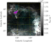 |
Fig. 16 Velocity gradients (cyan segments) overplotted on the NH map of the NCPL. Magenta segments correspond to our polarization measfrements. |
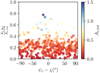 |
Fig. 17 Molecular fraction versus the relative difference between the POS H i velocity gradient angle (ψc) and the magnetic field orientation (χ), inferred from the Planck data. The colorbar shows the total Av. |
6 Discussion
We have employed a suite of observations to probe the magnetic field, kinematics, and chemical composition of a selected filamentary structure of the Ursa Major cirrus. We found a change in the relative orientation between the structure’s long axis and the magnetic field: the atomic subregion of the structure shows alignment, whereas a shift in the orientation occurs at the interface between H i and H2 media. Previous studies of the relative orientation have been statistical, binning observed/simulated data of multiple structures. Our approach complements these studies by providing a detailed look at the properties of one structure in the transition from atomic to molecular gas. By observing H i,12CO, and [C ii], we have established that the magnetic field changes orientation with respect to the gas morphology, as does the orientation of velocity gradients.
6.1 Magnetic field and H i alignment
6.1.1 Consequences for modeling Galactic foregrounds for cosmic microwave background studies
Clark et al. (2014, 2015) and Kalberla et al. (2016) compared the orientation of the POS component of the magnetic field with the orientation of H i filaments and found that at low column densities the two are statistically aligned. Based on this property, Clark & Hensley (2019) constructed a 3D map of the magnetized ISM over the full sky. In their map, the H i filament orientation was used to indirectly trace the POS magnetic field and the H i line radial velocity was used to disentangle the contribution from different magnetic field configurations along each LOS. The resulting map has been used to improve modeling of Galactic foreground emission in 3D (Pelgrims et al. 2021), a subject of high importance for cosmological studies (Tassis & Pavlidou 2015; Planck Collaboration Int. XXX 2016).
In contrast to what has been assumed in the aforementioned works, our polarization data suggest that in certain cases H i structure is not a good proxy for the POS magnetic field geometry. Even though the  structure of the target cloud is filamentary, the major axis of this filament shifts orientation with respect to the magnetic field (showing alignment in the parts of the structure that are atomic but forming near-orthogonal angles when the gas becomes molecular in Fig. 13). The results of Clark et al. (2014) and Kalberla et al. (2016) are statistical in nature and the alignment does not necessarily hold in individual cases, such as ours and in Skalidis et al. (2018).
An important result that comes up from our survey is that the alignment between the  structure and the magnetic field orientation becomes weak when molecular gas is present. Our polarization data follow the shape of the cloud, as traced by the total (both atomic and molecular) column density. This, in the context of the magnetic field modeling with H i data (Clark & Hensley 2019), indicates that the magnetic field orientation in clouds with significant H2 may not be accurately traced by the orientation of H i gas. If confirmed with observations at other transition clouds, the results of such modeling should be cautiously interpreted wherever the medium turns molecular. Such regions can be selected by maps like those from Planck Collaboration Int. XXIX (2016) or Kalberla et al. (2020). A conservative approach for mitigating biases in foreground modeling due to misalignment of filaments with magnetic fields would be to assign larger uncertainties for inferred magnetic field angles at regions that exhibit the presence of H2 above some thresholds. However, we note that the results of Clark & Hensley (2019) refer to much larger angular scales. Therefore, the potential misalignment caused by the presence of molecular gas (which is more spatially compact than the diffuse medium) may be statistically weaker when the averaging takes place.
6.1.2 Comparison with past works
The relative angle between the polarization orientation and the column density morphology of clouds has been a topic widely studied in the past few years. Soler et al. (2013) were the first to propose, using numerical simulations, that the relative orientation between the magnetic field and the major axis of filamentary structures changes from parallel to perpendicular as column density increases. Chen et al. (2016) proposed that the change happens when the Alfvén Mach number changes from sub-Alfvénic to super-Alfvénic. But subsequently Soler & Hennebelle (2017) and Seifried et al. (2020) found that the transition in their simulations happens for MA ≫ 1. Numerical simulations of Körtgen & Soler (2020) showed that this transition can also happen in high-density regions within a cloud, when turbulence is sub-Alfvénic, even if self-gravity is not included. Among these works, the simulated conditions are different, but all of them suggest that there is a threshold, in MA or n, above which the relative orientation between the magnetic field and the column density (or volume density) of the cloud changes.
Planck Collaboration Int. XXXII (2016) explored this transition using observations of polarized dust emission. They found that the transition happens, when log10(N) ≈ 21.7; their sample consisted mostly of regions with NH ~ 1021−1023 cm−2. Fissel et al. (2019) studied the young molecular cloud, Vela C, and found that the transition happens when n exceeds 103 cm−3, while Alina et al. (2019) concluded that there is an extra dependence on the relative orientation; it can vary according to the column density contrast between the filament and its background medium. More precisely, they found that the alignment of the magnetic field with the filamentary structures is prominent when the column density contrast is lower than NH < 4 × 1020 cm−2, while when a cloud exceeds this limit the relative orientations tend to become random. All these works, however, mainly focus on high-density (or column density) environments, whereas our cloud is a transition diffuse cloud.
In our target cloud, the maximum inferred density is 500 cm−3, while its maximum total column density is ~2 × 1021 cm−2. We found that the magnetic field orientation is relatively well correlated with the total column density (atomic and molecular) shape of the cloud (right panel in Fig. 13). This is consistent with all the aforementioned works that have shown that the relative orientation transition, from parallel to perpendicular, happens at much higher density and column density values.
6.2 Alternative magnetic field strength estimate
In the same cloud, Tritsis et al. (2019) estimated the magnetic field strength using a novel technique developed by Tritsis et al. (2018), which is based on the properties of the compressible MHD modes. This method assumes that the observed column density and velocity variations perpendicular to the mean magnetic field orientation is due to the propagation of fast magnetosonic waves. Tritsis et al. (2019) argued that the target cloud shares similar observational properties with striations, which are quasi-linear gas structures observed in molecular clouds (Goldsmith et al. 2008; Panopoulou et al. 2016; Tritsis & Tassis 2018) and likely formed by the magnetosonic waves (Tritsis & Tassis 2016). In addition, they assumed that the magnetic field is parallel to the H i structure, as suggested by Clark et al. (2014). Our atomic and molecular regions coincide with Region 1 and 2 in Tritsis et al. (2019), and hence we can directly compare our BPOs values with their estimates.
Tritsis et al. (2019) assumed that n = 10 cm−3; this, however, is inconsistent with our [C ii] observations (Sect. 3.1), which suggest that there the gas density is 50−100 cm−3. We rescaled their magnetic field strength using our density estimates. The magnetic field strength scales as B0 ∝  (Eq. (9)), and hence the rescaled values are
 (22)
(22)
where nours is our inferred density estimates, nTR19 is the density assumed by Tritsis et al. (2019), and  is their estimated magnetic field strength. In the atomic region, they found that
  . Using Eq. (22) we derive that the rescaled magnetic field strength values are
  ; we used our lower and upper nour estimates with their lower and upper
  limits in order to compute the rescaled magnetic field strength limits. Their estimated values are lower than what we inferred for the same region using our polarization measurements, which is
  (Table 2).
In the molecular region, Tritsis et al. (2019) estimated that  . But, we cannot directly compare our estimated values with theirs for two main reasons: Firstly, they assumed that the magnetic field orientation is parallel to the
  structure, while our polarization data revealed that the orientation of the field is almost perpendicular to the cloud in Figs. 2 and 12. Secondly, their estimates are solely based on H i data, while there is significant H2 gas there.
6.3 Magnetic field morphology and the H i velocity gradients
González-Casanova & Lazarian (2017) developed a novel technique for studying the ISM magnetized turbulence. It is called the velocity gradient technique (VGT) and is based on the properties of strong Alfvénic turbulence. This theory predicts that turbulent eddies form perpendicular to the local magnetic field orientation, and hence developing gas velocity gradients that are perpendicular to the mean magnetic field orientation. The same behavior can be obtained when large-scale flows of gas expand perpendicular to the magnetic field lines (e.g., Girichidis 2021). In either case, when self-gravity takes over the velocity gradients tend to become parallel to the magnetic field (e.g., Yuen & Lazarian 2017; Hu et al. 2019; Girichidis 2021).
In our target cloud, we found that the POS magnetic field orientation in the atomic subregion is perpendicular to the H i velocity gradients, while they tend to align close to the CO clump. We have argued that a large-scale expansion of H i gas has significantly affected the dynamics of our target cloud. Thus, it is more plausible that the magnetic field is perpendicular to the velocity gradients because of a large-scale expansion that compresses the magnetic field lines rather than because of Alfvénic distortions, as would be expected from the VGT. The alignment of the H i velocity gradients with the magnetic field close to the CO clump is probably caused by self-gravity. This alignment and the fact that our inferred density for the CO clump is ~400 cm−3 match very well with the results of Girichidis (2021), who suggested that self-gravity starts dominating at n ~ 400 cm−3.
6.4 The magnetic field strength versus density relation
The relation between the magnetic field strength and density is important for determining how dense cores collapse. Crutcher et al. (2010) found, using Zeeman data, that the maximum magnetic field strength scales as
 (23)
(23)
They concluded that the 2/3 scaling is consistent with spherically collapsing cores where the magnetic field has but a minor role in the cloud dynamics. However, their data are dominated by noise and in order to reach this conclusion they relied on several prior assumptions applied within a Bayesian framework (especially the underestimation of the uncertainties of the density estimates used). The 2/3 scaling was questioned by Tritsis et al. (2015) who concluded that the same data are better described by B ∝ n1/2; this scaling is consistent with the anisotropic core collapse model as presented by Mouschovias (1976a,b). Jiang et al. (2020) also showed that the results of Crutcher et al. (2010) are debatable since the Zeeman data are too noisy, and hence their analysis is dominated by statistical biases. Pattle & Fissel (2019) compiled archival polarization data and with the DCF method they found that their results are consistent with the scalings in Eq. (23). However, the scatter of B in their sample is an order of magnitude or more in some cases. Recently, Myers & Basu (2021) used polarization data toward 16 cores and they also found results consistent with Eq. (23). They concluded that their targeted cores are spherical but, contrary to Crutcher et al. (2010), that the magnetic field energy can be relatively large compared to the gravitational energy of the cores. Their analysis is based on the DCF method with the Q = 0.5 calibration factor found in numerical simulation (Ostriker et al. 2001; Padoan et al. 2001; Heitsch et al. 2001). However, the assumptions and the regime of applicability of the DCF method was recently questioned by Skalidis & Tassis (2021) and Skalidis et al. (2021). They found that DCF can be highly inaccurate in sub-Alfvénic or trans-Alfvénic turbulence even if the Q factor is applied, or if the method is combined with more sophisticated techniques, like the dispersion function analysis of Hildebrand et al. (2009) and Houde et al. (2009). Altogether, the current observational constraints of the B − ρ relation seem to be vague, because the results are either based on noisy data (Zeeman data, Crutcher et al. 2010) or high quality data (dust polarization) with uncertain methods (DCF, Pattle & Fissel 2019; Myers & Basu 2021).
Our inferred total magnetic field strength values are a factor of ~3 higher than the upper limit inferred by Crutcher et al. (2010) in Eq. (23). The maximum inferred density between the atomic and molecular region increases significantly, from ~100 to ~400 cm−3, but the magnetic field strength remains constant within our uncertainties11. Thus, there seems to be no correlation between the magnetic field strength and the gas density although the H i to H2 transition takes place between the two regions. This indicates that gas kinematics are dominated by flows along the magnetic field lines that accumulate gas and increase the gas density without increasing the strength of the field in this transition cloud.
7 Conclusion
We studied the role of the magnetic field in the H i-H2 transition in a diffuse ISM cloud toward the Ursa Major cirrus. We probed the magnetic field properties of the cloud using optical polarization and the gas properties of the cloud by performing CO spectroscopic observations that traced the J = 0−1, J = 1−2 lines and the 157.6 µm [C ii] emission line.
The target H i cloud is filamentary (Fig. 2). The cloud consists of two subregions: (1) the atomic, where gas is mostly atomic, and (2) the molecular, where molecular gas is most abundant. Toward the molecular subregion, we detected a CO clump and estimate its mean molecular fractional abundance to be  . We also find that there is a significant amount of hot (T ≈ 300–400 K) and dense (n ≈ 350–500 cm−3) CO-dark H2 gas at the edges of the cloud; CO-dark H2 seems to be more abundant than CO-bright H2 there.
Using our polarization data, we estimated the POS magnetic field strength using the method of Skalidis & Tassis (2021). In the atomic subregion, we estimate the POS magnetic field strength to be  ; this, combined with archival H i Zee-man data, yields a total magnetic field strength of
  . In the molecular subregion, the estimated magnetic field strength is
  µG, with the total strength being
  , which is consistent with the atomic subregion estimate within our uncertainties. We find no correlation between the magnetic field strength and the gas density between the two regions. This indicates that flows along the magnetic field lines tend to accumulate gas without affecting the magnetic field strength. The estimated Alfvén Mach number of the cloud is MA ≈ 1, which indicates that turbulence is trans-Alfvénic.
We compared the POS magnetic field orientation with the H i velocity gradients. We find that in the atomic subregion the local magnetic field tends to be perpendicular to the H i velocity gradients, while close to the CO clump velocity gradients tend to become parallel. The alignment between the two quantities probably marks the gravitational infall of the H i gas toward the clump. All these pieces of evidence are consistent with theoretical expectations. The shape of the CO clump is asymmetric, with an aspect ratio between its minor and major principal axis equal to 0.4. The mean polarization orientation is closer (24° offset) to the short axis of the clump. This also supports the notion that self-gravity is important for the molecular part of the cloud and is consistent with the observation that H i accumulates preferentially along the magnetic field lines.
We compared the POS magnetic field orientation with the  morphology of the cloud using the RHT algorithm (Clark et al. 2014). We find that the magnetic field is parallel to the H i structure of the cloud in the atomic region, while it tends to be perpendicular to the H i cloud structure in the molecular subregion; we provided evidence that this relative shift of the magnetic field orientation was probably caused by expanding gas. On the other hand, the magnetic field tends to form a smaller offset angle with the total column density structure of the cloud (NH) in both the atomic and molecular subregions. We conclude that the magnetic field morphology of the cloud is better correlated with the NH rather than the
  structure of the cloud.
Our target cloud lies at the edges of the NCPL, which is a large-scale expanding structure. Using archival data, we explored if there is a correlation between the relative difference of the magnetic field with the H i velocity gradients and the molecular abundance, as suggested by simulations (e.g., Girichidis 2021). We provided evidence that the molecular abundance is enhanced in regions where the magnetic field is parallel to the H i velocity gradients, probably because these are regions where self-gravity dominates. However, these results should be interpreted with caution since projection effects at these scales are important, and more work is required to further constrain this scenario.
Acknowledgements
We thank the anonymous referee for their careful and constructive comments. We thank P. F. Goldsmith, S. E. Clark, M. Shull, D. Seifried, A. Tritsis, M. Kopsacheili, and V. Pelgrims for fruitful comments on the manuscript. We are grateful to T. Diaz-Santos, D. Fadda, and R. Munch for their help with the SOFIA observations. We are also thank M.-A. Miville-Deschénes for informing us about the DHIGLS data, and J. Ingalls for sharing their ISO data. We appreciate the assistance of the PMO-13.7 m staff during the observations. Particularly, we would like to thank Jixian Sun for scheduling our supplementary observations with the PMO-13.7 m telescope on very short notice. We greatly thank Qing-zeng Yan for sharing his CO (J = 1−0) data prior to his publication. This project has received funding from the European Research Council (ERC) under the European Union’s Horizon 2020 research and innovation programme under grant agreement No. 771282. Y.G. was supported by the National Key R&D Program of China under grant 2017YFA0402702. This project has received funding from the European Union’s Horizon 2020 research and innovation programme under the Marie Sklodowska-Curie RISE action, grant agreement No 691164 (ASTROSTAT).
Appendix A Cloud distance
Optical dust polarization is a powerful tool for estimating the ISM cloud distances (e.g., Panopoulou et al. 2019a,b). Stars located in front of an ISM cloud will be un-polarized, because there is negligible dust material to polarize the starlight. On the other hand, starlight emitted from sources behind the cloud, will get linearly polarized as they pass through the cloud due to dichroic extinction (Anders son et al. 2015).
In Fig. A.1 we show the degree of polarization (biased) versus the star distances. Black dots indicate measurements with S/N ≥ 2.5, while blue dots correspond to upper limits. Some measurements located further than 1400 pc are not shown for visualization purposes. There is a step-like increase in the degree of polarization at ~300 − 400 pc and this indicates the cloud distance. There are some measurements with low S/N at further distances, but this could be caused by large uncertainties due to low exposures or because the magnetic field is inclined with respect to the LOS axis.
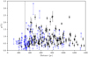 |
Fig. A.1 Degree of polarization versus star distance. Black dots indicate measurements with S/N≥ 2.5, blue dots measurements with S/N< 2.5. The plot has been truncated at 1400 pc for visualization purposes. The vertical line is at 310 pc. |
Appendix B Velocity gradient angles transformation to the Galactic reference frame
We used Eq. (18) to measure the H i velocity gradients toward the NCPL. This equation, however, measures the velocity gradients with respect to the horizontal axis of the target field and lie within the [−90°, +90°] range. On the other hand, the magnetic field orientation, as measured from Planck polarization data, are with respect to the North Galactic Pole (NGP), increasing toward the east. We transformed the H i velocity gradient angles (ψ0) to the NGP reference frame in order to compute their difference with the magnetic field orientation.
Figure B.1 shows the geometry of this transformation. The magenta box corresponds to the HI4PI field toward the NCPL; ψc is the velocity gradient angle measured with respect to the Cartesian x−y plane of the image. In order to compute ψ, which is the velocity gradient angle measured in the Galactic reference frame, we computed  ; this is the local angle between the x axis of the image and the coordinate grid. For the computation, we used Eq. (A9) from the appendix of Planck Collaboration Int. XIX (2015), which properly takes the local curvature of the grid into account. Then, we computed ψ as
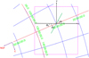 |
Fig. B.1 Velocity gradient angle transformation. The magenta box corresponds to the HI4PI field toward the NCPL, ψc is the velocity gradient angle measured with respect to the Cartesian x−y plane of the target field, |

 (B.1)
(B.1)
The derived ψ angle lies in the [0°, 180°] range.
Appendix C H i Gaussian decomposition
A characteristic fitted spectrum with ROHSA toward a random LOS along the NCPL is shown with the blue histogram in Fig. C.1. The individual Gaussian components fitted by ROHSA are shown with the black solid lines, while the red line is the total intensity of the fitted spectrum. In Fig. D.1 we show the five decomposed Gaussians used for the H i fitting of the NCPL spectra. The first, second, and third columns correspond to their zeroth-moment (intensity), first-moment (velocity centroid), and second-moment (velocity spread) maps, respectively.
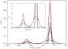 |
Fig. C.1 Characteristic H i spectrum fitted by ROHSA. The vertical axis is intensity measured in antenna temperature units (K), and the horizontal axis is the gas velocity in km s−1. The blue histogram denotes the observed H i emission spectrum and the red line the corresponding fit produced by ROHSA. The black lines show the individual Gaussian components of the spectrum decomposition. |
Appendix D Contribution of intensity fluctuations in velocity gradients
H i spectra may show multiple peaks that vary in intensity at small velocity intervals. For example, in Fig. C.1, the major peak at velocities close to 5 km s−1 is decomposed into three Gaussian components. Consider that each component corresponds to a distinct gas layer within the cloud, moving at different, but constant velocity. If the intensity of each component changes, because the gas column density changes, then the velocity gradients computed with Eq. (18) will be nonzero; however, this gradient would arise from changes in Tb, rather than velocity fluctuations.
In order to determine the relative contribution of the Tb fluctuations in the velocity gradients computation, we explored whether the intensities of the decomposed Gaussians are spatially correlated. If the Tb fluctuations between the different components are strongly correlated, then we can fit the spectrum with a single Gaussian, which is the sum of the individual components (as shown in Fig. C.1). In this case the Tb fluctuations are minor, and Vc gradients accurately represent the averaged gas kinematics. On the other hand, if Gaussian intensities are not correlated (or anticorrelated), then fluctuations of Tb between the different components can be significant; in this case one has to decompose the observed signal into distinct components.
We employed the H i Gaussian decomposition that we performed with ROHSA in Sect. 5. We computed the normalized correlation of the intensity maps (Tb) between the three decomposed Gaussians at velocities ~5 km s−1(Fig. C.1) toward our target cloud; the Tb maps of the individuals components are shown in the first column of the second, fourth, and fifth row in Fig. D.1. We computed the correlation between two intensity maps, Tb,A and Tb,B, as in Yuen et al. (2021),
 (D.1)
(D.1)
where  , and j = Tb,A, Tb,B. If the two decomposed intensity maps were perfectly correlated, then NCC(Tb,A, Tb,B) = 1; if they were anticorrelated NCC(Tb,A,Tb,B) = −1, while if they were uncorrelated, then NCC(Tb,A,Tb,B) = 0. We consider that two maps are strongly correlated when NCC(TA, TB) > 0.7. Our results are the following: the Tb maps correlation between the second and fourth Gaussian is NCC(Tb,A,Tb,B) = 0.87, between the second and fifth Gaussian is NCC(Tb,A,Tb,B) = 0.75, while between the fourth and fifth Gaussian is NCC(Tb,A, Tb,B) = 0.78. The Tb maps of the individual components are strongly correlated with each other. Thus, the observed H i spectrum toward the target cloud can be fitted with a single Gaussian component. This suggests that Tb fluctuations have but a minor contribution in the observed H i spectra. Thus, the H i velocity gradients, computed in Sect. 3.3, are an accurate proxy of the average kinematics of the cloud.
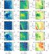 |
Fig. D.1 Different Gaussian components used for the fitting of the H i spectrum of the NCPL. Left column: Zeroth velocity moment map in antenna temperature units. Middle column: First-moment (centroid velocity) map measured in km s−1. Right column: Second-moment (velocity dispersion) map measured in km s−1. |
References
- Alina, D., Ristorcelli, I., Montier, L., et al. 2019, MNRAS, 485, 2825 [Google Scholar]
- Andersson, B. G., Lazarian, A., & Vaillancourt, J. E. 2015, ARA&A, 53, 501 [Google Scholar]
- Bailer-Jones, C. A. L., Rybizki, J., Fouesneau, M., Demleitner, M., & Andrae, R. 2021, AJ, 161, 147 [Google Scholar]
- Barinovs, G., van Hemert, M. C., Krems, R., & Dalgarno, A. 2005, ApJ, 620, 537 [NASA ADS] [CrossRef] [Google Scholar]
- Barriault, L., Joncas, G., & Plume, R. 2011, MNRAS, 416, 1250 [NASA ADS] [CrossRef] [Google Scholar]
- Beattie, J. R., Federrath, C., & Seta, A. 2020, MNRAS, 498, 1593 [Google Scholar]
- Bellomi, E., Godard, B., Hennebelle, P., et al. 2020, A&A, 643, A36 [NASA ADS] [CrossRef] [EDP Sciences] [Google Scholar]
- Bialy, S., Burkhart, B., & Sternberg, A. 2017, ApJ, 843, 92 [NASA ADS] [CrossRef] [Google Scholar]
- Bieging, J. H., & Peters, W. L. 2011, ApJS, 196, 18 [NASA ADS] [CrossRef] [Google Scholar]
- Bieging, J. H., Peters, W. L., & Kang, M. 2010, ApJS, 191, 232 [NASA ADS] [CrossRef] [Google Scholar]
- Bieging, J. H., Revelle, M., & Peters, W. L. 2014, ApJS, 214, 7 [NASA ADS] [CrossRef] [Google Scholar]
- Blagrave, K., Martin, P. G., Joncas, G., et al. 2017, ApJ, 834, 126 [Google Scholar]
- Blinov, D., Kiehlmann, S., Pavlidou, V., et al. 2021, MNRAS, 501, 3715 [NASA ADS] [CrossRef] [Google Scholar]
- Bolatto, A. D., Wolfire, M., & Leroy, A. K. 2013, ARA&A, 51, 207 [CrossRef] [Google Scholar]
- Bracco, A., Benjamin, R. A., Alves, M. I. R., et al. 2020, A&A, 636, L8 [NASA ADS] [CrossRef] [EDP Sciences] [Google Scholar]
- Chandrasekhar, S., & Fermi, E. 1953, ApJ, 118, 113 [Google Scholar]
- Chen, C.-Y., & Ostriker, E. C. 2014, ApJ, 785, 69 [NASA ADS] [CrossRef] [Google Scholar]
- Chen, C.-Y., & Ostriker, E. C. 2015, ApJ, 810, 126 [Google Scholar]
- Chen, C.-Y., King, P. K., & Li, Z.-Y. 2016, ApJ, 829, 84 [Google Scholar]
- Clark, S. E., & Hensley, B. S. 2019, ApJ, 887, 136 [NASA ADS] [CrossRef] [Google Scholar]
- Clark, S. E., Peek, J. E. G., & Putman, M. E. 2014, ApJ, 789, 82 [NASA ADS] [CrossRef] [Google Scholar]
- Clark, S. E., Hill, J. C., Peek, J. E. G., Putman, M. E., & Babler, B. L. 2015, Phys. Rev. Lett., 115, 241302 [Google Scholar]
- Colditz, S., Fumi, F., Geis, N., et al. 2012, in Ground-based and Airborne Instrumentation for Astronomy IV, eds. I.S. McLean, S.K. Ramsay, & H. Takami, 8446, International Society for Optics and Photonics (SPIE), 392 [Google Scholar]
- Crutcher, R. M., Nutter, D. J., Ward-Thompson, D., & Kirk, J. M. 2004, ApJ, 600, 279 [Google Scholar]
- Crutcher, R. M., Wandelt, B., Heiles, C., Falgarone, E., & Troland, T. H. 2010, ApJ, 725, 466 [NASA ADS] [CrossRef] [Google Scholar]
- Davis, L. 1951, Phys. Rev., 81, 890 [Google Scholar]
- Dawson, J. R., McClure-Griffiths, N. M., Kawamura, A., et al. 2011, ApJ, 728, 127 [NASA ADS] [CrossRef] [Google Scholar]
- Dickey, J. M., & Lockman, F. J. 1990, ARA&A, 28, 215 [Google Scholar]
- Fadda, D., & Chambers, E. T. 2018, in American Astronomical Society Meeting Abstracts, 231, 150.11 [NASA ADS] [Google Scholar]
- Fischer, C., Beckmann, S., Bryant, A., et al. 2018, J. Astron. Instrum., 7, 1840003 [Google Scholar]
- Fissel, L. M., Ade, P. A. R., Angilè, F. E., et al. 2019, ApJ, 878, 110 [CrossRef] [Google Scholar]
- Gaia Collaboration (Brown, A.G.A., et al.) 2021, A&A, 649, A1 [NASA ADS] [CrossRef] [EDP Sciences] [Google Scholar]
- Gillmon, K., Shull, J. M., Tumlinson, J., & Danforth, C. 2006, ApJ, 636, 891 [NASA ADS] [CrossRef] [Google Scholar]
- Girichidis, P. 2021, MNRAS, 507, 5641 [NASA ADS] [CrossRef] [Google Scholar]
- Girichidis, P., Walch, S., Naab, T., et al. 2016, MNRAS, 456, 3432 [NASA ADS] [CrossRef] [Google Scholar]
- Goldsmith, P. F. 2013, ApJ, 774, 134 [NASA ADS] [CrossRef] [Google Scholar]
- Goldsmith, P. F., Heyer, M., Narayanan, G., et al. 2008, ApJ, 680, 428 [Google Scholar]
- Goldsmith, P. F., Langer, W. D., Pineda, J. L., & Velusamy, T. 2012, ApJS, 203, 13 [Google Scholar]
- Goldsmith, P. F., Pineda, J. L., Langer, W. D., et al. 2016, ApJ, 824, 141 [CrossRef] [Google Scholar]
- Goldsmith, P. F., Pineda, J. L., Neufeld, D. A., et al. 2018, ApJ, 856, 96 [NASA ADS] [CrossRef] [Google Scholar]
- González-Casanova, D. F., & Lazarian, A. 2017, ApJ, 835, 41 [CrossRef] [Google Scholar]
- Green, G. M., Schlafly, E. F., Finkbeiner, D., et al. 2018, MNRAS, 478, 651 [Google Scholar]
- Grenier, I. A., Casandjian, J.-M., & Terrier, R. 2005, Science, 307, 1292 [Google Scholar]
- Heiles, C. 1989, ApJ, 336, 808 [NASA ADS] [CrossRef] [Google Scholar]
- Heiles, C., & Troland, T. H. 2003, ApJS, 145, 329 [Google Scholar]
- Heitsch, F., Zweibel, E. G., Mac Low, M.-M., Li, P., & Norman, M. L. 2001, ApJ, 561, 800 [Google Scholar]
- Heitsch, F., Stone, J. M., & Hartmann, L. W. 2009, ApJ, 695, 248 [NASA ADS] [CrossRef] [Google Scholar]
- HI4PI Collaboration (Ben Bekhti, N., et al.) 2016, A&A, 594, A116 [NASA ADS] [CrossRef] [EDP Sciences] [Google Scholar]
- Hildebrand, R. H., Kirby, L., Dotson, J. L., Houde, M., & Vaillancourt, J. E. 2009, ApJ, 696, 567 [Google Scholar]
- Houde, M., Vaillancourt, J. E., Hildebrand, R. H., Chitsazzadeh, S., & Kirby, L. 2009, ApJ, 706, 1504 [Google Scholar]
- Hu, Y., Yuen, K. H., Lazarian, V., et al. 2019, Nat. Astron., 3, 776 [NASA ADS] [CrossRef] [Google Scholar]
- Hu, Y., Lazarian, A., & Yuen, K. H. 2020, ApJ, 897, 123 [NASA ADS] [CrossRef] [Google Scholar]
- Ingalls, J. G., Reach, W. T., & Bania, T. M. 2002, ApJ, 579, 289 [NASA ADS] [CrossRef] [Google Scholar]
- Inoue, T., & Inutsuka, S.-I., 2008, ApJ, 687, 303 [NASA ADS] [CrossRef] [Google Scholar]
- Inoue, T., & Inutsuka, S.-I., 2009, ApJ, 704, 161 [NASA ADS] [CrossRef] [Google Scholar]
- Jiang, H., Li, H.-B., & Fan, X. 2020, ApJ, 890, 153 [NASA ADS] [CrossRef] [Google Scholar]
- Kalberla, P. M. W., Kerp, J., Haud, U., et al. 2016, ApJ, 821, 117 [Google Scholar]
- Kalberla, P. M. W., Kerp, J., & Haud, U. 2020, A&A, 639, A26 [EDP Sciences] [Google Scholar]
- King, O. G., Blinov, D., Ramaprakash, A. N., et al. 2014, MNRAS, 442, 1706 [NASA ADS] [CrossRef] [Google Scholar]
- Klein, R., Beckmann, S., Bryant, A., et al. 2014, in Ground-based and Airborne Instrumentation for Astronomy V, eds. S.K. Ramsay, I.S. McLean, & H. Takami, 9147, International Society for Optics and Photonics (SPIE), 1018 [Google Scholar]
- Körtgen, B., & Soler, J. D. 2020, MNRAS, 499, 4785 [CrossRef] [Google Scholar]
- Krumholz, M. R., Stone, J. M., & Gardiner, T. A. 2007, ApJ, 671, 518 [NASA ADS] [CrossRef] [Google Scholar]
- Kutner, M. L., & Ulich, B. L. 1981, ApJ, 250, 341 [NASA ADS] [CrossRef] [Google Scholar]
- Langer, W. D., Velusamy, T., Pineda, J. L., et al. 2010, A&A, 521, A17 [NASA ADS] [CrossRef] [EDP Sciences] [Google Scholar]
- Lazarian, A., & Yuen, K. H. 2018, ApJ, 853, 96 [NASA ADS] [CrossRef] [Google Scholar]
- Lord, S. D. 1992, A new software tool for computing Earth’s atmospheric transmission of near- and far-infrared radiation, NASA Technical Memorandum 103957 [Google Scholar]
- Marchal, A., Miville-Deschênes, M.-A., Orieux, F., et al. 2019, A&A, 626, A101 [NASA ADS] [CrossRef] [EDP Sciences] [Google Scholar]
- McCullough, P. R., & Benjamin, R. A. 2001, AJ, 122, 1500 [NASA ADS] [CrossRef] [Google Scholar]
- Meyerdierks, H., Heithausen, A., & Reif, K. 1991, A&A, 245, 247 [NASA ADS] [Google Scholar]
- Miville-Deschênes, M. A., Boulanger, F., Joncas, G., & Falgarone, E. 2002, A&A, 381, 209 [NASA ADS] [CrossRef] [EDP Sciences] [Google Scholar]
- Miville-Deschênes, M. A., Joncas, G., Falgarone, E., & Boulanger, F. 2003a, A&A, 411, 109 [NASA ADS] [CrossRef] [EDP Sciences] [Google Scholar]
- Miville-Deschênes, M. A., Levrier, F., & Falgarone, E. 2003b, ApJ, 593, 831 [Google Scholar]
- Monet, D. G., Levine, S. E., Canzian, B., et al. 2003, AJ, 125, 984 [Google Scholar]
- Mouschovias, T. C. 1976a, ApJ, 206, 753 [Google Scholar]
- Mouschovias, T. C. 1976b, ApJ, 207, 141 [CrossRef] [Google Scholar]
- Mouschovias, T. C. 1978, in IAU Colloq. 52: Protostars and Planets, eds. T. Gehrels, & M.S. Matthews, 209 [Google Scholar]
- Myers, P. C., & Basu, S. 2021, ApJ, 917, 35 [NASA ADS] [CrossRef] [Google Scholar]
- Myers, P. C., Goodman, A. A., Gusten, R., & Heiles, C. 1995, ApJ, 442, 177 [NASA ADS] [CrossRef] [Google Scholar]
- Naghizadeh-Khouei, J., & Clarke, D. 1993, A&A, 274, 968 [NASA ADS] [Google Scholar]
- Ntormousi, E., Dawson, J. R., Hennebelle, P., & Fierlinger, K. 2017, A&A, 599, A94 [NASA ADS] [CrossRef] [EDP Sciences] [Google Scholar]
- Ostriker, E. C., Stone, J. M., & Gammie, C. F. 2001, ApJ, 546, 980 [Google Scholar]
- Padoan, P., Goodman, A., Draine, B. T., et al. 2001, ApJ, 559, 1005 [Google Scholar]
- Panopoulou, G., Tassis, K., Blinov, D., et al. 2015, MNRAS, 452, 715 [Google Scholar]
- Panopoulou, G. V., Psaradaki, I., & Tassis, K. 2016, MNRAS, 462, 1517 [Google Scholar]
- Panopoulou, G. V., Hensley, B. S., Skalidis, R., Blinov, D., & Tassis, K. 2019a, A&A, 624, A8 [Google Scholar]
- Panopoulou, G. V., Tassis, K., Skalidis, R., et al. 2019b, ApJ, 872, 56 [NASA ADS] [CrossRef] [Google Scholar]
- Pattle, K., & Fissel, L. 2019, Front. Astron. Space Sci., 6, 15 [Google Scholar]
- Pelgrims, V., Clark, S. E., Hensley, B. S., et al. 2021, A&A, 647, A16 [NASA ADS] [CrossRef] [EDP Sciences] [Google Scholar]
- Pety, J. 2005, in SF2A-2005: Semaine de l’Astrophysique Francaise, eds. F. Casoli, T. Contini, J.M. Hameury, & L. Pagani, 721 [Google Scholar]
- Pineda, J. L., Goldsmith, P. F., Chapman, N., et al. 2010, ApJ, 721, 686 [NASA ADS] [CrossRef] [Google Scholar]
- Pineda, J. L., Langer, W. D., Velusamy, T., & Goldsmith, P. F. 2013, A&A, 554, A103 [CrossRef] [EDP Sciences] [Google Scholar]
- Pineda, J. L., Langer, W. D., Goldsmith, P. F., et al. 2017, ApJ, 839, 107 [NASA ADS] [CrossRef] [Google Scholar]
- Planck Collaboration XII. 2020, A&A, 641, A12 [NASA ADS] [CrossRef] [EDP Sciences] [Google Scholar]
- Planck Collaboration Int. XIX. 2015, A&A, 576, A104 [NASA ADS] [CrossRef] [EDP Sciences] [Google Scholar]
- Planck Collaboration Int. XXVIII. 2015, A&A, 582, A31 [NASA ADS] [CrossRef] [EDP Sciences] [Google Scholar]
- Planck Collaboration Int. XXIX. 2016, A&A, 586, A132 [NASA ADS] [CrossRef] [EDP Sciences] [Google Scholar]
- Planck Collaboration Int. XXX. 2016, A&A, 586, A133 [NASA ADS] [CrossRef] [EDP Sciences] [Google Scholar]
- Planck Collaboration Int. XXXII. 2016, A&A, 586, A138 [NASA ADS] [CrossRef] [EDP Sciences] [Google Scholar]
- Plaszczynski, S., Montier, L., Levrier, F., & Tristram, M. 2014, MNRAS, 439, 4048 [NASA ADS] [CrossRef] [Google Scholar]
- Pound, M. W., & Goodman, A. A. 1997, ApJ, 482, 334 [NASA ADS] [CrossRef] [Google Scholar]
- Ramaprakash, A. N., Rajarshi, C. V., Das, H. K., et al. 2019, MNRAS, 485, 2355 [NASA ADS] [CrossRef] [Google Scholar]
- Schlegel, D. J., Finkbeiner, D. P., & Davis, M. 1998, ApJ, 500, 525 [Google Scholar]
- Schmidt, G. D., Elston, R., & Lupie, O. L. 1992, AJ, 104, 1563 [Google Scholar]
- Seifried, D., Haid, S., Walch, S., Borchert, E. M. A., & Bisbas, T. G. 2020, MNRAS, 492, 1465 [NASA ADS] [CrossRef] [Google Scholar]
- Shan, W., Yang, J., Shi, S., et al. 2012, IEEE Trans. Terahertz Sci. Technol., 2, 593 [Google Scholar]
- Shull, J. M., Danforth, C. W., & Anderson, K. L. 2021, ApJ, 911, 55 [NASA ADS] [CrossRef] [Google Scholar]
- Skalidis, R., & Pelgrims, V. 2019, A&A, 631, A11 [Google Scholar]
- Skalidis, R., & Tassis, K. 2021, A&A, 647, A186 [NASA ADS] [CrossRef] [EDP Sciences] [Google Scholar]
- Skalidis, R., Panopoulou, G. V., Tassis, K., et al. 2018, A&A, 616, A52 [NASA ADS] [CrossRef] [EDP Sciences] [Google Scholar]
- Skalidis, R., Sternberg, J., Beattie, J. R., Pavlidou, V., & Tassis, K. 2021, A&A, 656, A118 [NASA ADS] [CrossRef] [EDP Sciences] [Google Scholar]
- Sofia, U. J., Lauroesch, J. T., Meyer, D. M., & Cartledge, S. I. B. 2004, ApJ, 605, 272 [NASA ADS] [CrossRef] [Google Scholar]
- Soler, J. D., & Hennebelle, P. 2017, A&A, 607, A2 [NASA ADS] [CrossRef] [EDP Sciences] [Google Scholar]
- Soler, J. D., Hennebelle, P., Martin, P. G., et al. 2013, ApJ, 774, 128 [Google Scholar]
- Sternberg, A., Le Petit, F., Roueff, E., & Le Bourlot, J. 2014, ApJ, 790, 10 [CrossRef] [Google Scholar]
- Sun, J. X., Lu, D. R., Yang, J., et al. 2018, Acta Astron. Sinica, 59, 3 [Google Scholar]
- Tassis, K., & Pavlidou, V. 2015, MNRAS, 451, L90 [NASA ADS] [CrossRef] [Google Scholar]
- Tassis, K., Dowell, C. D., Hildebrand, R. H., Kirby, L., & Vaillancourt, J. E. 2009, MNRAS, 399, 1681 [CrossRef] [Google Scholar]
- Tritsis, A., & Tassis, K. 2016, MNRAS, 462, 3602 [Google Scholar]
- Tritsis, A., & Tassis, K. 2018, Science, 360, 635 [Google Scholar]
- Tritsis, A., Panopoulou, G. V., Mouschovias, T.C., Tassis, K., & Pavlidou, V. 2015, MNRAS, 451, 4384 [NASA ADS] [CrossRef] [Google Scholar]
- Tritsis, A., Federrath, C., Schneider, N., & Tassis, K. 2018, MNRAS, 481, 5275 [Google Scholar]
- Tritsis, A., Federrath, C., & Pavlidou, V. 2019, ApJ, 873, 38 [NASA ADS] [CrossRef] [Google Scholar]
- Turnshek, D. A., Bohlin, R. C., Williamson, R. L.I., et al. 1990, AJ, 99, 1243 [NASA ADS] [CrossRef] [Google Scholar]
- Ulich, B. L., & Haas, R. W. 1976, ApJS, 30, 247 [Google Scholar]
- Vaillancourt, J. E. 2006, PASP, 118, 1340 [Google Scholar]
- Velusamy, T., Langer, W. D., Pineda, J. L., et al. 2010, A&A, 521, A18 [Google Scholar]
- Walch, S., Girichidis, P., Naab, T., et al. 2015, MNRAS, 454, 238 [Google Scholar]
- Wiesenfeld, L., & Goldsmith, P. F. 2014, ApJ, 780, 183 [Google Scholar]
- Yuen, K. H., & Lazarian, A. 2017, ApJ, 837, L24 [NASA ADS] [CrossRef] [Google Scholar]
- Yuen, K. H., Ho, K. W., & Lazarian, A. 2021, ApJ, 910, 161 [NASA ADS] [CrossRef] [Google Scholar]
The telescope is operated by the Arizona Radio Observatories, a division of Steward Observatory at the University of Arizona.
This is the median of the kinetic temperature distribution over a large sample of diffuse clouds in our Galaxy (Heiles & Troland 2003).
Orientations are measured with respect to the horizontal axis of Fig. 10 increasing counterclockwise.
This is a lower limit for the volume density, since we have found that the volume density in the molecular subregion of the current cloud can be up to 350 cm−3 (Sect. 3.1).
We applied the same analysis to data with better than 1° accuracy, but they were too noisy and we found no clear trend. We also tested these results using a larger smoothing radius and the results were similar to Fig. 17.
This is true even if we assumed a prolate 3D shape for the CO clump and that its depth is comparable to its minor axis, which is ~0.5 pc. In that case, the estimated density of the CO-bright region would be ~1150 cm−3, which yields a magnetic field that is ~25 µG; this is also consistent with the magnetic field strength estimate for the atomic region.
All Tables
All Figures
|
Fig. 1 Brightness temperature versus gas velocity. The black histogram corresponds to the H i emission spectrum, magenta to 12CO (j = 1−0), and cyan to 12CO (J = 2−1). The antenna temperature of H i is shown on the left vertical axis and the CO lines on the right vertical axis. The size of each bin is equal to the spectral resolution of each spectrum, i.e., 0.82, 0.16, and 0.32 km s−1 for H i, CO (J = 1−0), and CO (J = 2−1) emission lines, respectively. These spectra were extracted from RA, Dec = 09:33:00, +70:09:00. |
| In the text | |
|
Fig. 2 H i column density map of the target cloud. Colored segments correspond to the RoboPol polarization data with S/N ≥ 2.5 that trace the POS magnetic field. Blue and yellow segments correspond to measurements included in the estimation of the magnetic field strength in the atomic and molecular region, respectively. Red segments correspond to measurements with S/N ≥ 2.5 but were not used in the estimation of BPOS (Sect. 3.2). Measurements with S/N < 2.5 are shown with red circles. The radius of each circle corresponds to the observed polarization fraction. A scale segment and circle are shown in the top-right corner. Colored stars correspond to the C+ LOSs from both ISO (orange, black, and yellow) and SOFIA (green, blue, red, and cyan). The size of each star is much larger than the field of view of the instruments. Light green contours correspond to the CO (J = 1−0) integrated intensity at the 3, 5, and 9 K km s−1 levels. The black contours show the CO (J = 2−1) integrated intensity at the 2 and 4 K km s−1 levels. The dashed and solid orange polygons show the CO J = 1−0 and J = 2−1 surveyed regions, respectively. |
| In the text | |
|
Fig. 3 [C ii] emission line spectra of the four LOSs from the SOFIA FIFI-LS spectrometer. The continuum-subtracted fluxes are shown with the histograms. The color of each histogram corresponds to the LOS marked with the same colored star in Fig. 2. Light magenta corresponds to the transmission atmospheric model and the dark magenta histogram to the transmission model convolved with the instrumental spectral resolution. The solid black line corresponds to the Gaussian fit. The blue-shaded region shows the level of the continuum rms. |
| In the text | |
|
Fig. 4 [C ii] emission line spectra, Iλ, versus λ, obtained with ISO (Ingalls et al. 2002). The amplitude of continuum fluctuations is shown with light blue. The solid black lines correspond to the Gaussian fits of the C+ emission line. |
| In the text | |
|
Fig. 5 CO (J = 1−0) spectra toward the three LOSs overlapping with our SOFIA data. The horizontal axis is the velocity in the LSR. The labels show the spectrum coordinates. The color of each spectrum corresponds to the LOS shown with colored stars in Fig. 2. |
| In the text | |
|
Fig. 6 [C ii] integrated intensity versus H i column density. Colored lines show the expected [C ii] intensity assuming that both H i and H2 contribute to the ionization of carbon (see Eq. (6)) with varying temperature, gas density, and molecular fractional abundance. Colored points correspond to the colored-star LOSs shown with the same color in Fig. 2. |
| In the text | |
|
Fig. 7 Same as in Fig. 6. Points correspond to the colored-star LOSs shown with the same color in Fig. 2. |
| In the text | |
|
Fig. 8 Column densities of different species across the main ridge of the cloud. The color of the horizontal tick labels matches with the colored-star LOSs shown in Fig. 2. The red line corresponds to |
| In the text | |
|
Fig. 9 Distribution of polarization angles and their observatinal uncertianties. Top-left panel: dispersion of polarization angles for the atomic region. The solid cyan profile corresponds to the fitted Gaussian. The mean (µ), standard deviation (σ), and amplitude (α) of the fit are (µ, σ, α) = (63°, 18°, 9). Top-right panel: polarization angle error distribution. Bottom panels: same as for the upper panels, but for the molecular region. The free parameters of the fitted Gaussian are (µ, σ, α) = (12°, 15°, 8). |
| In the text | |
|
Fig. 10 Velocity gradients overplotted on the |
| In the text | |
|
Fig. 11 CO (J = 1−0) integrated intensity. White lines mark the major and minor axis of the CO clump. Red segments show the polarization measurements as in Fig. 2. The long red line at the center of the core corresponds to the mean magnetic field orientation. |
| In the text | |
|
Fig. 12 Our starlight polarization measurements (cyan segments) overplotted on the RHT output image. The colorbar shows the normalized intensity measured from the RHT. Stars and CO contours have the same meanings as in Fig. 2. |
| In the text | |
|
Fig. 13 Distribution of relative orientations. Left panel: distribution of the difference between the orientation of the |
| In the text | |
|
Fig. 14 Magnetic field morphology overplotted on the Planck-based NH map of the NCPL. Left panel: dust emission polarization rotated by 90°, shown by red segments. The length of each segment is proportional to the polarized intensity. Magenta segments correspond to our polarization measurements; all segments have a fixed size for visualization purposes. There is an offset in the magnetic field orientation as traced by optical and submillimeter polarization due to the large beam difference between the two observables. Colored stars correspond to the target C+ LOSs, as shown in Fig. 2. Right panel: zoomed-in view of the region toward the target cloud. The solid cyan segment shows the Hα canal found by McCullough & Benjamin (2001). |
| In the text | |
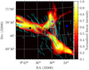 |
Fig. 15 RHT output for the NH map of our target cloud. Symbols have the same meanings as in Fig. 12. |
| In the text | |
|
Fig. 16 Velocity gradients (cyan segments) overplotted on the NH map of the NCPL. Magenta segments correspond to our polarization measfrements. |
| In the text | |
|
Fig. 17 Molecular fraction versus the relative difference between the POS H i velocity gradient angle (ψc) and the magnetic field orientation (χ), inferred from the Planck data. The colorbar shows the total Av. |
| In the text | |
|
Fig. A.1 Degree of polarization versus star distance. Black dots indicate measurements with S/N≥ 2.5, blue dots measurements with S/N< 2.5. The plot has been truncated at 1400 pc for visualization purposes. The vertical line is at 310 pc. |
| In the text | |
|
Fig. B.1 Velocity gradient angle transformation. The magenta box corresponds to the HI4PI field toward the NCPL, ψc is the velocity gradient angle measured with respect to the Cartesian x−y plane of the target field, |
| In the text | |
|
Fig. C.1 Characteristic H i spectrum fitted by ROHSA. The vertical axis is intensity measured in antenna temperature units (K), and the horizontal axis is the gas velocity in km s−1. The blue histogram denotes the observed H i emission spectrum and the red line the corresponding fit produced by ROHSA. The black lines show the individual Gaussian components of the spectrum decomposition. |
| In the text | |
|
Fig. D.1 Different Gaussian components used for the fitting of the H i spectrum of the NCPL. Left column: Zeroth velocity moment map in antenna temperature units. Middle column: First-moment (centroid velocity) map measured in km s−1. Right column: Second-moment (velocity dispersion) map measured in km s−1. |
| In the text | |
Current usage metrics show cumulative count of Article Views (full-text article views including HTML views, PDF and ePub downloads, according to the available data) and Abstracts Views on Vision4Press platform.
Data correspond to usage on the plateform after 2015. The current usage metrics is available 48-96 hours after online publication and is updated daily on week days.
Initial download of the metrics may take a while.