| Issue |
A&A
Volume 602, June 2017
|
|
|---|---|---|
| Article Number | A70 | |
| Number of page(s) | 16 | |
| Section | Interstellar and circumstellar matter | |
| DOI | https://doi.org/10.1051/0004-6361/201730387 | |
| Published online | 15 June 2017 | |
Distribution of water in the G327.3–0.6 massive star-forming region⋆
1 Max-Planck-Institut für Radioastronomie, Auf dem Hügel 69, 53121 Bonn, Germany
e-mail: sleurini@mpifr-bonn.mpg.de
2 INAF – Osservatorio Astronomico di Cagliari, via della Scienza 5, 09047 Selargius (CA), Italy
3 Laboratoire d’astrophysique de Bordeaux, Univ. Bordeaux, CNRS, B18N, allée Geoffroy Saint-Hilaire, 33615 Pessac, France
4 SRON Netherlands Institute for Space Research, PO Box 800, 9700 AV Groningen, The Netherlands
5 Kapteyn Astronomical Institute, University of Groningen, 9712 Groningen, The Netherlands
6 Kavli Institut for Astronomy and Astrophysics, Yi He Yuan Lu 5, HaiDian Qu, Peking University, 100871 Beijing, PR China
7 Leiden Observatory, Leiden University, PO Box 9513, 2300 RA Leiden, The Netherlands
8 Max-Planck-Institut für Extraterrestrische Physik, Giessenbachstrasse 1, 85748 Garching, Germany
Received: 2 January 2017
Accepted: 17 March 2017
Aims. Following our past study of the distribution of warm gas in the G327.3–0.6 massive star-forming region, we aim here at characterizing the large-scale distribution of water in this active region of massive star formation made of individual objects in different evolutionary phases. We investigate possible variations of the water abundance as a function of evolution.
Methods. We present Herschel/PACS (4′× 4′) continuum maps at 89 and179 μm encompassing the whole region (Hii region and the infrared dark cloud, IRDC) and an APEX/SABOCA (2′× 2′) map at 350 μm of the IRDC. New spectral Herschel/HIFI maps toward the IRDC region covering the low-energy water lines at 987 and 1113 GHz (and their H218O counterparts) are also presented and combined with HIFI pointed observations toward the G327 hot core region. We infer the physical properties of the gas through optical depth analysis and radiative transfer modeling of the HIFI lines.
Results. The distribution of the continuum emission at 89 and 179 μm follows the thermal continuum emission observed at longer wavelengths, with a peak at the position of the hot core and a secondary peak in the Hii region, and an arch-like layer of hot gas west of this Hii region. The same morphology is observed in the p-H2O 111–000 line, in absorption toward all submillimeter dust condensations. Optical depths of approximately 80 and 15 are estimated and correspond to column densities of 1015 and 2 × 1014 cm-2, respectively, for the hot core and IRDC position. These values indicate an abundance of water relative to H2 of 3 × 10⁻⁸ toward the hot core, while the abundance of water does not change along the IRDC with values close to some 10-8. Infall (over at least 20″) is detected toward the hot core position with a rate of 1−1.3 × 10⁻²M⊙ /yr, high enough to overcome the radiation pressure that is due to the stellar luminosity. The source structure of the hot core region appears complex, with a cold outer gas envelope in expansion, situated between the outflow and the observer, extending over 0.32 pc. The outflow is seen face-on and rather centered away from the hot core.
Conclusions. The distribution of water along the IRDC is roughly constant with an abundance peak in the more evolved object, that is, in the hot core. These water abundances are in agreement with previous studies in other massive objects and chemical models.
Key words: stars: formation / stars: protostars / ISM: molecules / line: profiles
© ESO, 2017
1. Introduction
In the past years, several studies have focused on the characterization of water, a crucial molecule in modeling the chemistry and the physics of molecular clouds (van Dishoeck et al. 2014), in different environments of star formation. In particular, the key program Water In Star-forming regions with Herschel (WISH; van Dishoeck et al. 2011) targeted different phases of star and planet formation to understand the evolution of water in these sources, while other Herschel projects also investigated water in selected sources (e.g., Emprechtinger et al. 2013; Santangelo et al. 2014; Leurini et al. 2014; Goicoechea et al. 2015). Most of these studies focus on observations of single sources and do not contain much spatial information on the distribution of water in the environment surrounding the source. Exceptions are the work of Jacq et al. (2016), which covered the clouds surrounding the mini-starburst W43 MM1, or studies of large-scale molecular outflows (e.g., Nisini et al. 2013; Santangelo et al. 2014), but in these cases, only the immediate surrounding of low-mass young stellar objects was investigated.
Herschel/HIFI observed water line transitions (toward the hot core region in pointing mode).
As part of the WISH project, six nearby cluster-forming clouds were mapped in multiple water transitions; the data were complemented with mid- and high-J CO and 13CO observations with the APEX telescope and Herschel to better characterize the warm gas in the (proto-) clusters. In this paper, we present observations of water of the star-forming region G327.3–0.6 at a distance of 3.1 kpc (Wienen et al. 2015). Different evolutionary phases of massive star formation coexist in a small (~3 pc) region (Wyrowski et al. 2006): a bright Hii region (Goss & Shaver 1970) associated with a luminous photon-dominated region seen in CO (hereafter Paper I, Leurini et al. 2013), and a chemically extremely rich hot core (Nummelin et al. 1998; Gibb et al. 2000) in a cold infrared dark cloud hosting several other dust condensations (Minier et al. 2009), one of which has signs of active star formation (Cyganowski et al. 2008). The region was studied in mid-J CO and 13CO lines in Paper I: emission is detected over the whole extent of the maps (3 × 4 pc) with excitation temperatures ranging from 20 K up to 80 K in the gas around the Hii region, and H2 column densities from a few 1021 cm-2 in the interclump gas to 3 × 1022 cm-2 toward the hot core. The warm gas is only a small percentage (~10%) of the total gas in the infrared dark cloud, while it reaches values of up to ~35% of the total gas in the ring surrounding the Hii region. The goal of our current study is to characterize the large-scale distribution of water in an active region of massive star formation that shows different evolutionary phases to verify whether its abundances varies as a function of evolution.
2. Observations and data reduction
We present mapping observations of the G327.3–0.6 massive star-forming region collected with the HIFI (de Graauw et al. 2010) and PACS (Poglitsch et al. 2010) spectroscopic instruments on board Herschel1 (Pilbratt et al. 2010) in the framework of the WISH program. Additional APEX observations with the SABOCA camera (Sect. 2.3) are also discussed.
2.1. HIFI pointed observations and maps
Three water lines as well as the 13CO(10–9) (Leurini et al. 2013) and C18O(9–8) lines have been observed with HIFI in August 2010 (OD 461) and February 2011 (OD 645) using the on-the-fly observing mode with Nyquist sampling. The center of the map is αJ2000 = 15h53m05.48s, δJ2000 = −54°36′06.2′′. The reference position was 5 arcmin offset north in declination for all observations.
The HIFI observations were made in bands 4B and 4A. The sideband separation of 8 GHz and IF bandwidth of 4 GHz allow a local oscillator (LO) setting where the o-H2O and H218O 111–000 transitions at 1113.343 GHz and 1101.698 GHz, respectively, and the 13CO(10–9) transition at 1101.350 GHz can be observed simultaneously. The same holds for the p-H2O and C18O (9–8) transitions at 987.927 GHz and 987.560 GHz, respectively. The 1113 GHz water map consists of 19 OTF rows made of 26 independent points covering 3.5′ × 2.7′ (one map coverage), while the 987 water map consists of 8 OTF rows made of 10 independent points covering 1.2′ × 1.2′ (with two map coverages).
As with all massive protostars observed by the WISH GT-KP, 14 water lines (see Table 1) were observed with HIFI in the pointed mode at frequencies between 547 and 1670 GHz in 2010 and 2011 (list of observation identification numbers, obsids, are given in Table 1) toward the G327 hot core region (RA = 15h53m08.8s, Dec = –54°37′01′′), between SMM2 and the hot core position (see Sect. 3.3) because of a confusion between different references (e.g., Bergman 1992). An additional high-energy water line at 970.3150 GHz was also observed. We used the double beam-switch observing mode with a throw of 3′. The off positions were inspected and did not show any emission. The frequencies, energy of the upper levels, system temperatures, integration times, and rms noise level at a given spectral resolution for each of the lines are provided in Table 1.
Data were taken simultaneously in H and V polarizations using both the acousto-optical Wide-Band Spectrometer (WBS) with 1.1 MHz resolution and the digital auto-correlator or High-Resolution Spectrometer (HRS), which provides higher spectral resolution. Calibration of the raw data into the TA scale was performed by the in-orbit system (Roelfsema et al. 2012); conversion to Tmb was made using the latest beam efficiency estimate from October 20142 given in Table 1 and a forward efficiency of 0.96. HIFI receivers are double sideband with a sideband ratio close to unity (Roelfsema et al. 2012). The flux scale accuracy is estimated to be between 10% for bands 1 and 2, 15% for bands 3 and 4, and 20% in bands 6 and 71. The frequency calibration accuracy is 20 kHz and 100 kHz (i.e., better than 0.06 km s-1) for HRS and WBS observations, respectively. Data calibration was performed in the Herschel Interactive Processing Environment (HIPE, Ott 2010) version 12. Further analysis was made within the CLASS3 package (Dec. 2015 version). These lines are not expected to be polarized, therefore data from the two polarizations were averaged together after inspection. For all observations, eventual contamination from lines in the image sideband of the receiver was checked and none was found. Some unidentified features (not due to water species) are nevertheless detected but not blended with the water lines. Because HIFI is operating in double-sideband, the measured continuum level was divided by a factor of 2 (in the figures and tables) to be directly compared to the single-sideband line profiles (this is justified because the sideband gain ratio is close to 1).
Summary of the PACS Herschel and SABOCA APEX observations.
2.2. PACS maps
PACS is an integral field unit with a 5 × 5 array of spatial pixels (hereafter spaxels). Each spaxel covers  , providing a total field of view of ~47″ × 47″. The observations (see Table 2, obsid 1342192145) were performed using the PACS chopped line spectroscopic mode (see Poglitsch et al. 2010). The area mapped with PACS is shown in Fig. 1. This mode achieves a spectral resolution of ~0.12 μm (corresponding to a velocity resolution of ~210 km s-1). Two nod positions were used that chopped 6’ on each side of the source. The two positions were compared to assess the influence of the off-source flux of observed species from the off-source positions. The typical pointing accuracy is better than 2′′.
We performed the basic data reduction with the Herschel interactive processing environment v.12 (HIPE, Ott 2010). The flux was normalized to the telescope background and calibrated using Neptune observations. Spectral flatfielding within HIPE was used to increase the signal-to-noise ratio (for details, see Herczeg et al. 2012; Green et al. 2016). In order to account for the substantial flux leakage between the spaxels surrounding the true source position and to improve the continuum stability, custom IDL routines were used to further process the datacubes for the wavelength-dependent loss of radiation for a point source (see PACS Observers Manual). The overall flux calibration is accurate to ~20% based on the flux repeatability for multiple observations of the same target in different programs, cross-calibrations with HIFI and ISO, and continuum photometry. The continuum (and line) rms are given in Table 2.
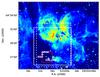 |
Fig. 1 Large-scale Spitzer image at 3.6 μm of G327.36–0.6. The boxes show the areas mapped with PACS at 89 and 179 μm (solid white line), with HIFI at 1113 GHz (white dashed line), and at 987 GHz (red line). The white crosses and triangle mark the positions discussed in Paper I. |
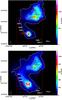 |
Fig. 2 Color scale and white contours are the PACS continuum image of G327.36–0.6 at 89 (top panel, resolution is 9.1″) and 179 μm (bottom panel, resolution is 12.3″). Contours are from 5% of the peak flux in steps of 10%. The triangles mark the positions of the submillimeter continuum peaks reported in Table 3. The red box outlines the area plotted in Fig. 3. |
2.3. SABOCA map
The IRDC in G327.36–0.6 was observed with the APEX4 telescope in the continuum emission at 350 μm with the Submillimeter APEX Bolometer Camera (SABOCA, Siringo et al. 2010). The observations were performed in 2010, on May 11 (see Table 2). The pointing was checked on B13134 (also used as flux calibrator) and on the bright hot core hosted in the IRDC, on the peak of the 3 mm continuum emission obtained by Wyrowski et al. (2008) with the ATCA array. Skydips (fast scans in elevation at constant azimuthal angle) were performed to estimate the atmospheric opacity. The weather conditions at the time of the observations were good, with a median precipitable water vapor level of 0.24 mm. The data were reduced with the BOA software (Schuller 2012).
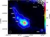 |
Fig. 3 Distribution of the SABOCA continuum emission at 350 μm along the infrared dark cloud in G327.3–0.6. Contours are from 5% of the peak flux in steps of 10%. The triangles mark the positions of the submillimeter continuum peaks reported in Table 3. The red cross marks the position observed for the single pointing HIFI observations. The white circle in the bottom left corner shows the beam of the SABOCA observations. |
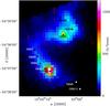 |
Fig. 4 Distribution of the continuum emission at 179 μm in G327.3–0.6 (color scale). The solid red contours represent the distribution of the absorption in the 111 → 000 p-H2O line, integrated in the velocity range vLSR = [−55,−37] km s-1 (from –3σ, –4.5 K km s-1, in steps of –3σ). Labels are the peaks of the 450 μm continuum emission from Minier et al. (2009). |
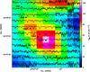 |
Fig. 5 Spectral HIFI map of the line-to-continuum ratio of the 111 → 000 p-H2O line toward the IRDC region overlaid on the 13CO(6–5) integrated emission (color image). The temperature axis ranges from –1 to 1.5 K, the velocity axis ranges from –65 to –35 km s-1. The 13CO(6–5) data are smoothed to the resolution of the H2O map. The black triangles mark the positions of the peaks of the 450 μm continuum emission. |
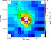 |
Fig. 6 Integrated HIFI intensity map of the p-H2O 202-111 line ([−50,−38 ] km s-1) toward the IRDC region (color image). The black contours show the SABOCA continuum emission at 350 μm from 5% of the peak flux in steps of 10%. The triangles mark the positions of the submillimeter continuum peaks reported in Table 3. Beams of the observations of the p-H2O 202-111 line (white circle) and of the 350 μm continuum (red circle) are shown in the bottom left corner. |
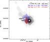 |
Fig. 7 Integrated intensity map of the p-H2O 202-111 line in the blue- ([−60,−50 ] km s-1, blue contours from 30% of the peak emission in steps of 10%) and redshifted ([−35,−15 ] km s-1, red contours from 30% of the peak emission in steps of 10%) velocity ranges toward the IRDC region. The gray contours represent the integrated intensity of C18O(9–8) ([−48,−42 ] km s-1, from 50% of the peak emission in steps of 10%). The white triangles mark SMM1 and SMM2, the green cross the position observed in the single-pointing HIFI observations (labeled as outflow in Fig. 8.) The dotted lines outline the cuts used to derive the P-V diagrams discussed in Sect. 3.2.1). |
3. Observational results
3.1. Continuum emission
Figure 2 shows the distribution of the continuum emission of G327.3–0.6 at 89 and 179 μm observed with PACS. The morphology follows the thermal continuum emission observed at larger wavelengths (Schuller et al. 2009; Minier et al. 2009), with a peak at the position of the hot core and a secondary peak in the Hii region toward SMM3. Additionally, the 179 μm map also shows weak emission along an arch-like layer of hot gas west of the Hii region seen in Fig. 1 at 3.6 μm but also in 12CO and 13CO (Paper I). The SABOCA map of the IRDC in the G327.3–0.6 massive star-forming region is shown in Fig. 3. The map shows a shift toward the east with respect to the continuum map at 450 μm published by Minier et al. (2009). However, the peak of the 350 μm continuum emission coincides with the position derived for the hot core in Paper I and with the position inferred with interferometric measurements at 3 mm (Wyrowski et al. 2008) within ~1.̋3, while the peak of the 450 μm continuum map is shifted of (7′′, –2.6′′) from the ATCA position. Therefore the difference between the two continuum maps is probably due to a pointing error in the 450 μm data (larger than their pointing accuracy), which then have been shifted.
We used the Gauss-clump program (Stutzki & Güsten 1990; Kramer et al. 1998) to derive the positions of the dust condensations discussed by Minier et al. (2009). Their new coordinates are reported in Table 3 together with other sources in the region discussed in Paper I and in this study. The largest offset is for SMM6, whose SABOCA position is (–6.̋1, –5.̋6) from the previous reported one, although the source is well isolated. The other sources (SMM1, SMM2, SMM4, SMM7, and SMM8) have a shift (compared to Minier et al. 2009) between –4.̋3 and –7.̋0 in right ascension, and between –1.̋9 and 2.̋5 in declination from the corresponding 450 μm sources. For the region not covered by our SABOCA map, the coordinates listed in Table 3 are from Minier et al. (2009).
3.2. Large-scale distribution of water
The distribution of the absorption in the p-H2O 111–000 line is shown in Fig. 4 and closely follows the distribution of the continuum emission at 179 μm. The detailed distribution of water in the IRDC and the Hii regions are discussed in Sects. 3.2.1 and 3.2.2, respectively.
3.2.1. IRDC
The IRDC hosting the hot core G327.3–0.6 was mapped in two different transitions of water (at 987 and 1113 GHz) with HIFI. Absorption is detected in the 1113 GHz line toward all submillimeter dust condensations (see Fig. 5), but because it is saturated toward most positions, any quantitative analysis is difficult (see Sect. 4.1). The 202−111 line at 987 GHz (see Fig. 6) is seen in emission except at the positions of the hot core and of SMM2, where a combination of emission and absorption is detected. The ground-state para line shows a broad saturated absorption toward the hot core position, and its line-width narrows along the IRDC. On the other hand, the 987 GHz line shows broad blue- and redshifted non-Gaussian wings. The integrated intensity maps of the red- (vLSR = [−35,−15] km s-1) and blueshifted (vLSR = [−60,−50] km s-1) 987 GHz line show a bipolar morphology along the north-south direction centered to the east of the hot core near SMM2 (see Fig. 7). This shift is not due to a pointing error in the HIFI observations as the C18O(9–8) line (νC18O(9−8) = 987 560.3822 MHz, observed simultaneously to the 987 GHz water line) peaks on the hot core. The outflow is unresolved, and the blue- and redshifted emission is detected only in a few spectra centered approximately on (–10′′, –7′′) from the hot core. Figure 8 shows the P-V diagrams of the CO(6–5) line (from Paper I, top panels) and of the 987 GHz water transition (bottom panels) along two cuts in the north-south direction passing through the center of the outflow (left panels) and through the hot core (right panels). No obvious difference is seen in the CO(6–5) transition in the two P-V diagrams, while the 987 GHz transition shows broader profiles (extending approximately up to –15 km s-1 ) along the axis of the outflow than in the north-south cut through the hot core. This is also seen in Fig. 9, where we show the 987 GHz and CO(6–5) (averaged over the HIFI beam) spectra at the peak of the redshifted emission: the water profile has a clear non-Gaussian redshifted wing and is self-absorbed, while CO(6–5) is not and has a broad non-Gaussian profile but no redshifted asymmetry. That the line-profile is broader in water than in CO (generally not seen in other sources using the CO(3–2) line, see van der Tak et al. 2013) could point to a molecular outflow in an earlier evolutionary phase of SMM2 than of the hot core. Recent observations of low-mass YSOs (Kristensen et al. 2012; Mottram et al. 2017) found that molecular outflows from class 0 YSOs have more prominent wings in water than those of class I sources.
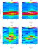 |
Fig. 8 Top: color scale and contours show the P-V diagram of the CO(6–5) transition computed along a vertical cut passing through the outflow a) and the hot core position b). Bottom: color scale and contours show the P-V diagram of the 202−111 H2O line computed along a vertical cut passing through the outflow c) and the hot core position d). The cut through the outflow position is from |


The 1113 GHz spectra show additional absorption features that are due to foreground clouds (van der Tak et al. 2013). From single-pointing deep integration observations of the 1113 GHz line toward the hot core (see Sect. 3.3), at least four features are detected at about − 16.6,−12.8,−11.4, and − 3.6 km s-1. When averaging on several pixels, the − 16.6 km s-1 absorption is detected toward SMM8 (and the other positions). The − 12.8 and − 11.4 km s-1 absorptions are detected at SMM1, SMM2, SMM4, SMM7, and SMM8, while the − 3.6 km s-1 component is not at SMM7 and SMM8. Estimating the exact size of the foreground clouds is impossible with our data: the line-of-sight clouds are mostly seen in absorption only toward the hot core and the other main dust condensations and therefore only toward the continuum emission. We can nevertheless indicate a lower limit of their extent: 20″, 35″, 55″, and 55″ for the foreground clouds at − 3.6,−16.6,−12.8, and − 11.4 km s-1, respectively.
In addition to these HIFI maps, the 212−101 line at 179.5 μm is detected with PACS in absorption over the entire extent of the IRDC. However, the line is spectroscopically unresolved and no further kinematical information can be derived from the PACS data, whereas the line is spectrally resolved by the HIFI pointed observation toward the hot core. Finally, the 303–212 transition at 174.6 μm, thus involving excited states, is detected in absorption toward the hot core, then revealing high gas density (see Sect. 4.2). Baseline instabilities prevent us from detecting the line at other positions.
3.2.2. Hii region
The distribution of the 1113 GHz transition in the G327.3–0.5 Hii region is shown in Fig. 11a, where its spectral map is overlaid on the integrated intensity of the 13CO(6–5) line from Paper I. The line profile is complex and shows a combination of emission and absorption. Two features are detected in absorption at ~− 50 and ~− 38 km s-1. Interestingly, the emission detected in H2O is always redshifted compared to the 13CO(10–9) line (Fig. 11b), which was observed simultaneously to the 1113 GHz line (presented in Leurini et al. 2013). The 13CO(10–9) seems to be associated with the absorption at ~− 50 km s-1 and peaked at the same velocity as the CO lines observed in Leurini et al. (2013). In Fig. 10 we compare the (r−v) diagrams of water and 12CO(6–5). These diagrams suggest that the emission feature at 1113 GHz traces the peak of the 12CO(6–5) emission. In Paper I we speculated that the CO emission is associated with an expanding shell. The two absorption features detected toward the center of the Hii region could be interpreted as due to the back and the front of the expanding shell. Their separation in km s-1 would be equal to twice the expansion velocity of the shell. The emission feature would be in the direction of the bright borders and would represent the mean velocity of the Hii region. However, the absolute velocities of water do not seem to fit those of CO (see Fig. 10): the velocity of the Hii region would be around − 45 km-1 and not around − 50 km-1, as originally suggested from the analysis of the CO isotopologs, and the expanding velocity would be slightly higher (6.5 instead of 5 km s-1).
In the PACS data (see Fig. A.1), the 179.5 μm line is detected in absorption toward all positions where continuum emission is seen, while the 174.6 μm line is not detected. Additionally, the CH+ (2–1) transition at 1669.281 GHz is also clearly detected in emission at several positions around the Hii region where CH+ traces a photon-dominated region.
3.3. Pointed observations of the hot core
The pointed observations were not performed toward the exact hot core position of G327 (see Sect. 2.1), but we nevertheless refer to this position as hot core hereafter. The observed position is 7.5″ west of SMM2 and 16″ northeast of SMM1. As a consequence, the o-H2O 221–212 and 212−101 (and the o-H217O 212–101) line observations are missing most of the water around SMM1, while for the other lines both SMM2 and SMM1 are covered by the beam.
The spectra including continuum emission are shown in Fig. 12 for the rare isotopologs (the H217O, H2 18O) and H216O. Spectra of the H2O 111–000 (and H2 18O), 202–111, and 212–101 lines have previously been presented by van der Tak et al. (2013). We show the HRS spectra, but for several lines (most of the ground-state lines) we used WBS spectra because the velocity range covered by the HRS was insufficient. For each transition, we derived the peak (emission or absorption dip) main-beam and continuum temperatures, half-power line widths for the different line components from multi-component Gaussian fits, made with the CLASS software, and opacities for lines in absorption (line parameters are given in Table 4).
Several foreground clouds (van der Tak et al. 2013) contribute to the spectra in terms of water absorption at Vlsr (–3.7, –11.4, –13, –16.6 km s-1) shifted with respect to the source velocity in the o-H2O 110–101, p-H2O 111–000, o-H2O 212–101 and p-H218O 111–000 line spectra.
The velocity components are attributed to cavity shocks and envelope component as for low-mass (LM) protostars (Mottram et al. 2014) or for other high-mass studies (see Herpin et al. 2016). The broad (FWHM ≃ 20–35 km s-1) velocity component arises in cavity shocks (i.e., shocks along the cavity walls) as its narrower version, the medium component (FWHM ≃ 5–10 km s-1), coming from a thin layer (1–30 AU) along the outflow cavity where non-dissociative shocks occur. The envelope component (narrow component with FWHM< 5 km s-1) is characterised by small FWHM and offset, that is, emission from the quiescent envelope.
In the following we refer to the commonly assumed hot core velocity of ~− 45 km s-1 (Bisschop et al. 2013), but (APEX) observations of rare CO isotopologs instead point to lower velocities: –43.7, –44.3, and –44.7 km s-1 for C18O J = 8–7 (and 13CO 10-9), 6–5, and 13CO 6–5, respectively (Rolffs et al. 2011; Leurini et al. 2013). Interestingly, the higher excitation lines tend to be more blueshifted.
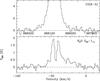 |
Fig. 9 Spectra of the 987 GHz water line (bottom panel) and of CO(6–5) (top panel) at the peak of the red-shifted integrated intensity of the 987 GHz transition. The CO(6–5) spectrum is averaged over the 987 GHz beam. |
3.3.1. Rare isotopologs
The para ground-state line of the H217O and H218O (see Fig. 12) is detected and exhibits the same line profile in absorption, made of an envelope component (FWHM ~ 3 km s-1) slightly blueshifted (less than 1 km s-1) from the APEX VLSR, one narrowormedium redshifted component in absorption, and a broader absorption that is more redshifted (by ≤10 km s-1). This broad absorption is discussed in Sect. 6.1. A similar profile is observed for the o-H217O 212–101 line. While the o-H217O 110–101 line is not detected, the o-H218O 110–101 line is tentatively detected with a weak and narrow absorption at –49.8 km s-1.
In contrast, a relatively strong signal is observed for the p-H218O 202–111 and o-H218O 312–303 transitions (see Fig. 12) showing the same cavity shock blueshifted component in emission. In addition, the p-H218O 202–111 line exhibits an absorption at –51 km s-1 similar to the one observed for the ground-state lines. We note that the o-H218O 312–303 line is blended with a CH3OH line.
The absorption that is either narrow (o-H218O 110–101, p-H218O 202–111, p-H218O 111–000), medium (p-H217O 111–000), or broad (p-H218O 111–000, p-H217O 111–000, o-H217O 212–101) observed at velocities between –49.1 and –54 km s-1 is most likely the broad absorption component seen in the NH3 line profile (at –49.62 km s-1 with Δv ≃ 11.1 km s-1) by Wyrowski et al. (2016) and could be due to absorption by foreground material (see Sect. 5.2 for a detailed discussion).
3.3.2. Water lines
All targeted H216O lines have been detected in absorption for the ground-state and the 221–212 lines, while other transitions exhibit a line profile in emission with some self-absorption at the source velocity. One line, p-H2O 524–431, is in pure emission (cavity shock component), but is blended with a methanol line.
An envelope component in absorption is seen in all lines but the p-H2O 524–431 and o-H2O 110–101transitions, centered at ~–43 km s-1. The medium cavity shock component is observed in absorption for the ground-state lines, redshifted by 2–4 km s-1, while it is seen in emission for the other water line and roughly at the source velocity. In addition, a broad component (up to 30 km s-1) is seen in emission in most of the lines (Sect. 6.1) and is blueshifted.
All H216O lines in absorption are optically thick based on line/continuum ratios (with opacities between 1 and 6, see Table 4). The optically thick p-H2O 202–111, p-H2O 211–202, and o-H2O 312–303 lines are strongly blue asymmetric, that is to say, they exhibit inverse P-Cygni profiles, hence they probably indicate infalling material.
3.3.3. Carbon species
In addition to the water lines, a few lines from carbon species have been observed and are shown in Fig. 13: 13CO J = 10–9, C18O J = 9–8, and CS J = 11–10. These three lines are in emission and centered at –44.8 km s-1, hence at a slightly redshifted velocity compared to what derived Rolffs et al. (2011) and Leurini et al. (2013) from ground observations. Line profiles exhibit a cavity shock component of 5.3–6.5 km s-1, but a broader component (FWHM ~ 11 km s-1) is also observed for the 13CO J = 10–9 line.
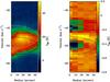 |
Fig. 10 (r−v) diagrams of the Hii region G327.3–0.5 obtained from the 12CO(6–5) (left) and from the 111–000-p H2O (right) data cubes. The radius axis is the distance to the shell expansion center, chosen to be the peak of the cm continuum emission. The black solid half-ellipse represents an ideal shell in (r−v) diagram with an expansion velocity of 5 km s-1 centered on –50 km s-1, the dashed white half-ellipse an ideal shell with an expansion velocity of 6.5 km s-1 centered on –45 km s-1. |
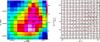 |
Fig. 11 Left: HIFI map of the 111 → 000 p-H2O line toward the Hii region overlaid on the 13CO(6–5) integrated emission (see Paper I). The temperature axis ranges from –1 to 1.5 K. The spectra are continuum subtracted. The 13CO(6–5) data are smoothed to the resolution of the H2O map. The triangle marks the Hii region from Paper I. Right: spectral maps of the 111 → 000 p-H2O line (black) and of the 13CO(10–9) transition (red). In both panels, the velocity axis ranges from –65 to –35 km s-1. |
Observed line emission parameters for the detected lines with HIFI toward G327-0.6 hot core pointed position.
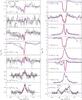 |
Fig. 12 HIFI spectra of the H217O/H218O (left) and H216O (right) lines (in black), with continuum for G327.3–0.6 hot core pointed position. The best-fit model with varying (from line to line) and constant (2.6 km s-1) turbulent velocity is shown as a red and dashed blue line above the spectra. Vertical dotted lines indicate the VLSR (–43.2 km s-1 from the line modeling). The spectra have been smoothed to 0.2 km s-1, and the continuum is divided by a factor of two. |
4. Analysis
4.1. Water abundance from the HIFI data
The opacity of a spectrally resolved unsaturated absorption line can be determined by![\begin{equation} \label{tau} \tau = -{\rm ln}\biggl[\frac{T_{\rm L}}{T_{\rm C}}\biggr] , \end{equation}](/articles/aa/full_html/2017/06/aa30387-17/aa30387-17-eq125.png) (1)where TL/TC is the line-to-continuum ratio. In this case, the column density of the absorbing species can be derived by (for ground-state lines, assuming negligible excitation)
(1)where TL/TC is the line-to-continuum ratio. In this case, the column density of the absorbing species can be derived by (for ground-state lines, assuming negligible excitation)  (2)In the case of the 1113 GHz transition, the absorption is saturated toward all positions in the IRDC. In addition, the corresponding H2 18O line (observed in the same setup as the main isotopolog line) is not detected in the HIFI maps. Therefore, the opacity of the 1113 GHz line cannot be computed analytically from Eq. (1). In this case, the optical depth can be derived from a curve-of-growth analysis, once the equivalent width, W, of the transition is computed. We have
  (3)where κ(ν is the absorption coefficient. We solved it graphically with a normal curve-of-growth analysis (log(W) vs. log(tau)).
The distribution of W in the IRDC is shown in Fig. 14. Results toward the Hii region are not reliable given the complex line profile of the 1113 GHz transition in this part of the source (see Fig. 11a). In the IRDC, W decreases steeply from a value of ~10 km s-1 toward the hot core down to a value of 5 km s-1 at the edge of the IRDC.
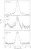 |
Fig. 13 HIFI spectra of 13CO J = 10–9, C18O J = 9–8, and CS J = 11–10 lines for the HIFI pointed position. The spectra have been smoothed to 0.2 km s-1. The vertical dotted line indicates the source velocity derived from Gaussian fitting, i.e., –44.8 km s-1. |
To derive the opacity of a transition from a curve-of-growth analysis, the line profile must be known. Line profile and line width of the 1113 GHz transition cannot be inferred from our data as the line is highly saturated. As first approximation, we can assume that the 1113 GHz line has the same profile and line width as the C18O(3–2) transition, which has a low opacity and a low energy (Eu ~ 32 K) and therefore is likely to trace the same cold component that absorbs water. We note that the width of H O cannot be used because the rare isotopolog line is not detected out of the central region. C18O(3–2) was observed by Wyrowski et al. (2006), and it has Gaussian profiles and typical widths of 4 kms-1 at the IRDC position and of 6 km s-1 at the hot core. For comparison, the width of the narrow component of the H218O 111−000 line is around 3 km s-1 at the hot core position, but the line profile also exhibits a broad component in absorption in the blue part that is due to the outflow. At the hot core position, the equivalent width of the 1113 GHz line is ~10. This value corresponds to an optical depth of 80 for Δv = 6 kms-1. However, for this value of W, the results are strongly dependent on the adopted line width and vary between 70 and 130 for Δv in the range 5–7 kms-1, with higher opacities corresponding to narrower line widths. At the IRDC position, W ~ 5 corresponds to an optical depth of ~15, and it does not substantially change with the line width. The validity of these estimates can be cross-checked on the hot core, where the deeper single-point observations of the 1113 GHz line allow us to detect the H218O and H
 O isotopologs of the line. From Eq. (1), we derive an optical depth of ~0.16 for the 111–000 p-H218O line, and of ~0.05 for the 111−000 p-H217O line. These values translate into lower limits of 62–87 for the optical depth of the main isotopolog line, in agreement with the result from the curve-of-growth method, assuming 16O/18O = 390 and 18O/17O = 4.5, respectively (Wilson & Rood 1994).
Equation (2) translates (assuming an o/p ratio of 3) into a total column density of water of 1 × 1015 cm-2 for the hot core for an optical depth of 80 and a line width of 6 km s-1. At the IRDC position, the column density of H2O is 2 × 1014 cm-2 for τ = 15 and Δν = 5 km s-1. In Paper I, we derived the distribution of the H2 column density over the whole region from CO and 13CO(6–5) maps. We can assume that CO and 13CO(6–5) trace the same gas that is absorbing the 1113 GHz transition and derive the abundance of water in the region. Toward the hot core, the H2 column density is 3.0× 1022 cm-2, while it decreases to 1.0 × 1022 cm-2 at the IRDC position5. These values correspond to abundances of water relative to H2 of 3× 10⁻⁸ toward the hot core, and 2 × 10⁻⁸ at the IRDC position. However, the uncertainties on these values are large, especially at the hot core position, where the strong saturation in the 1113 GHz line does not allow a precise determination of NH2O. Given the inferred range of opacities of the 1113 GHz line at this position, the abundance of water could vary between 3× 10⁻⁸ (for Δν = 4 km s-1) and 8 × 10⁻⁸ (for Δν = 7 km s-1).
Our observations suggest that the abundance of water does not change along the IRDC with values close to a few times 10-8. This abundance is consistent with results from several studies toward the outer part of envelopes around massive YSOs and in the foreground clouds (e.g., Snell et al. 2000; Bergin & Snell 2002; Emprechtinger et al. 2013), and with chemical models (e.g., Doty et al. 2002).
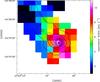 |
Fig. 14 Distribution of the equivalent width of the 111 → 000 p−H2O line in the IRDC. The black contours show the SABOCA continuum emission at 350 μm from 5% of the peak flux in steps of 10%. |
4.2. Kinetic temperature from PACS data
The PACS data suffer from two problems that make their analysis difficult: low spectral resolution and flux leakage. The latter arises because the PACS spaxels have a projected size of 9.̋4×9.̋4 on the sky, while the point-spread function of the Herschel telescope at 179.5 μm is approximately 12.̋6. For a point-like source that is perfectly centered on one spaxel, 44% of the flux is recovered at 179 μm (Fig. 7 of the PACS spectroscopy performance and calibration document6). However, the flux loss depends on the source structure for extended sources. In this case, the fraction of flux seen by PACS can be inferred only by deconvolving a source model image by the PACS point-spread function and comparing the flux seen in this synthetic observations with the original one in the model. This procedure should be performed for the continuum emission and for the absorption/emission of each transition separately, as the fraction of the flux recovered by PACS depends on the structure of the source in that particular tracer. Unfortunately, for G327.3–0.6 we do not have any continuum image at higher angular resolution than that of the PACS data to input as source model, nor we have any detailed knowledge of the distribution of water. Moreover, the approach described by Herczeg et al. (2012) and Karska et al. (2013) of summing up fluxes from adjacent spaxels is impractical in our case as different spaxels most likely see different sources given the complexity and the distance of the region.
Since the 179.5 μm and the 174.6 μm water lines are seen in absorption, the line-to-continuum ratio would not be affected by flux leakage if the two transitions had the same distribution of the continuum emission at the corresponding wavelength. We could test this assumption at 179.5 μm toward the position observed with HIFI in the o-H2O 212−101 line. This coincides with the position reported by Bergman (1992), shifted by approximately (8.̋7, 5.̋5) from the current hot core position. The comparison between the PACS and the HIFI 179.5 μm line at this position infer a difference of about 10% between the equivalent width of the water line obtained in the same velocity range, which value is indeed comparable to the relative calibration error between the two instruments. This test confirms that the PACS continuum and spectral observations at 179.5 μm are affected by flux loss in a similar way, but it is impossible to quantify this.
Assuming that there is no flux leakage, from the absorption of o-H2O 303–212 line at 174.6 μm, we can estimate an upper limit to the excitation temperature of the line, as this must be lower than the continuum temperature at 174.6 μm. The continuum level toward the hot core is approximately 1300 Jy/spaxel, which corresponds to a brightness temperature of 3.6 K, using a beam size of 12.̋3. At these wavelengths, and for typical temperatures of star-forming regions, the Rayleigh-Jeans approximation is not valid anymore, and the (exact) Planck brightness temperature is 21 K, implying a lower excitation temperature for the o-H2O 303–212 line. Since the critical density of this transition is very high, its excitation temperature depends mostly on the kinetic temperature of the medium and on the column density of ortho water. According to the RADEX online radiative transfer code (van der Tak et al. 2007), for a column density of 1014 cm-2 and a line-width of 6 km s-1 (see Sect. 4.1), an upper limit of 20 K for the excitation temperature of 303–212 line implies an upper limit to the kinetic temperature of 40 K, in agreement with the excitation temperature of 30–35 K for the hot core inferred in Paper I from CO(6–5) observations. The upper limit to the kinetic temperature of the gas increases with column density, and corresponds to 30 K for No−H2O = 1013 cm-2 and to 150 K for No−H2O = 5 × 1014 cm-2.
5. Modeling of the HIFI lines
This section intends to model the full line profiles in a single spherically symmetric model with different kinematical components that are due to turbulence, infall and outflow.
5.1. Method
The envelope temperature and density structure for the hot core from van der Tak et al. (2013) is used as input to the 1D radiative transfer code RATRAN (Hogerheijde & van der Tak 2000) in order to simultaneously reproduce all the water line profiles, following the method of Herpin et al. (2012). The H2O collisional rate coefficients are from Daniel et al. (2011). We assume a single source within the HIFI beam throughout our analyis, but we know that this source consists of two objects (SMM1, ~3770 M⊙ , and SMM2, ~200 M⊙ , see Minier et al. 2009 and Sect. 3.1), separated by ~23′′, and that our observations are pointing between these two objects (see Sect. 2.1). The insufficient knowledge of the SED for each of these subsources and the lack of spectral information prevent any more detailed modeling of the structure. Since SMM1 is ~20 times more massive than SMM2, we may assume that the emission is dominated by SMM1.
Adopting here a single-source structure that encompasses the substructure within the HIFI beam, the source model has two gas components: an outflow and the protostellar envelope. The outflow parameters, intensity, and width come from the Gaussian fitting presented in Sect. 3.3 for the broad component. The envelope contribution is parametrized with three input variables: water abundance (χH2O), turbulent velocity (Vtur), and infall velocity (Vinf). The width of the line is adjusted by varying Vtur. The line asymmetry is reproduced by the infall velocity. The line intensity is best fit by adjusting a combination of the abundance, turbulence, and outflow parameters. We adopt the following standard abundance ratios (same ratios for all the lines): 4.5 for H218O/the H217O (Thomas & Fuller 2008), and 3 for ortho/para-H2O. Based on Wilson & Rood (1994), the H216O/H218O abundance ratio is assumed to be 390. The model assumes a jump in the abundance in the inner envelope at 100 K because the ice mantles evaporate. All details about the method are given in Herpin et al. (2012).
5.2. Abundance and kinematics results
The analysis presented in Sect. 3.3 has shown that the width of the velocity components is not the same for all lines (e.g., half-power line widths from 2.4 to 4.9 km s-1 for the narrow component, see Table 4). As a consequence, a model with equal velocity parameters for all lines does not fit the data well. A turbulent velocity of 1.5 and 2.1 km s-1 for the H217O and H218O ground-state lines in absorption also gives a good result for the H216O lines in absorption. In contrast, a higher turbulent velocity of 2.6–3 km s-1 is needed for the lines in emission. We note that from RATRAN modeling of the NH332 +–22 − line, Wyrowski et al. (2016) derived a turbulent velocity of 2.3 km s-1. We then ran a model with a constant turbulence of 2.6 km s-1 for all lines (the best compromise we obtained after exploring a range of values). We also tested two other options that do not improve the fit significantly (see Fig. 12): the first option is a turbulence varying with radius following Herpin et al. (2012) and Herpin et al. (2016), the second option adjusts the turbulence line by line based on what is observed. The limiting factor rather seems to be the assumed spherical symmetry.
All modeled lines are centered at roughly − 43 ± 0.5 km s-1. The infall velocity is estimated to be –3.2 km s-1 (at ~1500 AU). A foreground absorption was included at − 48 ± 0.5 km s-1 with a width of 7.5 km s-1 for the ground-state water lines, but this component has no effect on the water abundance, very likely because it is sufficiently far from the source velocity. What we see is the absorption of the blue part of the outflow. This broad absorption has been observed and described in Herpin et al. (2016) for high-mass protostellar sources NGC 6334IN and DR21(OH). Interestingly, this absorption is at a similar velocity to one of the absorption features observed in the Hii region (see Sect. 3.2.2) and could be the same cloud over the whole region (see discussion in the next section). We did not try to reproduce the outflow absorption seen in p-H218O 111–000 and p-H217O 111–000 lines.
The water abundance is constrained by the modeling of the entire set of observed lines. Only a few lines (o-H218O 312–303, p-H2O 524–431 and o-H2O 312–303) are optically thin enough to probe the inner part of the envelope, part of all water line profiles is produced by water excited in the inner part and is revealed by the high spectral resolution of these observations. The H216O abundances relative to H2 are 5.2 × 10⁻⁵ in the inner part where T> 100 K, while the outer abundance (where T< 100 K) is 4 × 10⁻⁸ (we estimate the uncertainty to 30%), consistent with what we found in Sect. 4.1 for this position. No deviation from the standard o/p ratio of 3 is found.
6. Discussion
6.1. Source structure and dynamics of the hot core region
The broad absorption observed on the blue part of the H218O and the H217O para and ortho ground-state line profiles can give us some interesting information concerning the outer source structure. When we overplot these lines on the line of the main isotopolog (see Figs. 15 and 16), it first appears that the H217O and H218O line profiles are identical (within the noise): the broad absorption seems to be present only in the blue part; this is what we assumed in Sect. 3.3 for the Gaussian fitting. Conversely, the H216O profile differs with (weak) emission throughout most of the blue velocity interval (~–72 to –53 km s-1). From these observations we can first infer that this the H217O and H218O material is dense and cold enough to absorb the warmer outflowing gas and that it is situated between the outflow and us. In adddition, the fact that the outflow is preferentially absorbed in its blue part most likely reveals a cold outer gas envelope in expansion. Figure 17 shows the Gaussian fitting for the p-H218O 111–000 line when we assume that the absorption is rather centered on the source velocity: we obtain a component at –45 km s-1 whose FWHM is 34 km s-1.
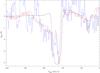 |
Fig. 15 Spectra of p-H218O 111–000 (× 6.2, in red) and p-H217O 111–000 (× 21, in blue) lines overplotted on the p-H2O 111–000 spectrum (in black). The spectra have been smoothed to 0.3 km s-1 (1.4 km s-1 for the H217O spectrum). |
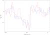 |
Fig. 16 Spectra of o-H217O 212–101 (× 0.3, in blue) line overplotted on the p-H217O 111–000 spectrum (in red). The spectra have been smoothed to 1.4 km s-1. |
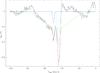 |
Fig. 17 Spectra of p-H218O 111–000 line (in black) showing the different Gaussian components used to fit the line (red = green+blue+purple). |
Assuming the peak intensity ratio (~6.2) of the H216O/H218O main narrow absorption features at –43.2 km s-1 (see Table 4) is valid for this broad absorption as well, we extrapolated the corresponding absorption in the p-H2O 111–000 line profile. We then tried to remove this Gaussian absorption. The resulting water line profile is shown on Fig. 18 and reveals a strong outflow centered at –44 km s-1 whose FWHM is 39 km s-1, broader than the first estimate we made in Sect. 3.3.
This cold absorbing material most likely corresponds to the cold clump found by Wyrowski et al. (2006) in N2H+ and located 30″ (0.4 pc) northeast of the hot core, but extending well over our HIFI pointed observed area (see Fig. 19). The velocity of this cloud is –45.9 km s-1, comparable to what we deduce here. Of course the line width in N2H+ is narrower than in water as a result of excitation mechanisms. This cold absorbing material could also be compatible with an expanding shell on the Hii region (see Fig. 10) centered at –45 km s-1. When we consider the distance between the Hii region and SMM1 (110 arcsec = 1.65 pc), the time needed to cross this distance from the center of the expanding Hii to SMM1 (at a velocity of 6.5 km s-1, see Sect. 3.2.2) would be 2.6 × 10⁵ yr.
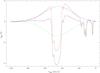 |
Fig. 18 Resulting line profile (in red) of the p-H2O 111–000 line corrected from the absorption shown in green and derived from the p-H218O 111–000 Gaussian line fitting. The original spectra are shown in black. The blue curve is the Gaussian fitting of the outflow. |
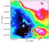 |
Fig. 19 APEX images from Wyrowski et al. (2006) in the N2H+ (3–2) and the CH3OH lines (red and black contours) overlaid on the 8 μm GLIMPSE emission. Embedded GLIMPSE point sources with massive YSO characteristics are marked with triangles. The Herschel 1113 GHz beam is indicated by the white circle centered on the HIFI observed position. |
We used RADEX online7 to investigate the excitation conditions for the derived H216O broad absorption. In perfect agreement with Wyrowski et al. (2006), we deduce Tkin = 18 K, nH2 = 106 cm-3, and NH2 = 1024 cm-2 for the cold cloud (χH2O = 4 × 10⁻⁸ is assumed). If the density is constant over the cloud, the absorbing material should extend over 6.7 × 10⁴ AU. Because the absorption is stronger for the blue part of the spectra, we propose that the outflow is seen face-on behind a cold envelope in expansion, as shown in Fig. 20.
As explained in Sect. 3.3, the HIFI observed position is centered between SMM2 and SMM1, and so are maybe some of the physical components derived from our model. Interestingly, Fig. 7 shows that the outflow is indeed rather centered away from the hot core, closer to the peak of the thermal CH3OH emission detected by Wyrowski et al. (2006; see Fig. 19) and might be associated to the class I methanol masers detected by Voronkov et al. (2014) between SMM1 and SMM2.
6.2. Accretion rate and water content
From the infall velocity estimated from our model (–3.2 km s-1 as revealed by the 752 GHz H216O line), using nH2 = 107 cm-3, we deduce a mass infall rate of 1−1.3 × 10⁻²M⊙ /yr. When we consider a mass of 20 M⊙ within a radius of 100 R⊙, this implies an accretion luminosity Lacc ~ 104L⊙ , which is high enough to overcome the radiation pressure that is due to the stellar luminosity (i.e., ~3. × 10-4M⊙ /yr). Nevertheless, it is important to stress that this accretion luminosity is very sensitive to the assumed density and radius, and as a consequence, this comparison has to be cautiously considered. The accretion rate is roughly three times greater than the rate derived by Wyrowski et al. (2016) from the NH332 +–22 − line, but twice lower than the free-fall accretion (if we assume that the entire envelope mass is collapsing). We tried to estimate the size of the infall region as revealed by p-H2O 202–111 line emission, but the line quickly vanishes out of the central source in the corresponding map. We derived a minimum size of the infall region of 20″ to be compared with the size of the cool (Tk = 20−100 K) envelope, that is, 80″. Moreover, we did not find any evidence of rotation.
The inner water abundance (5.2 × 10⁻⁵) derived in Sect. 5.2 for the hot core is slightly higher than what has been found for mid-IR-quiet massive protostars by Herpin et al. (2016). When we consider the high infall velocity we estimated for this source (–3.2 km s-1), this value agrees with the scenario proposed by Herpin and collaborators that higher inner abundance are observed for higher infall orexpansion velocities in the protostellar envelope. We also estimate the amount of water in the inner (T> 100 K) and outer regions to be 2.1 × 10⁻³ and 5.1 × 10⁻⁴M⊙ , respectively. This inner region that holds 80% of the water corresponds to the compact area of 2″ where Gibb et al. (2000) and Bisschop et al. (2013) situated most of the organic species they observed, coming from the grain mantle evaporation.
7. Conclusions
We have presented new Herschel/PACS continuum maps at 89 and 179 μm that encompass the whole region (Hii region and IRDC) and APEX/SABOCA map at 350 μm of the IRDC. These maps were combined with new spectral Herschel/HIFI maps toward the IRDC region at 987 and 1113 GHz. In addition, we analyzed and modeled HIFI pointed observations of 15 water lines toward the G327 hot core region.
Our data show that the distribution of the continuum emission at 89 and 179 μm follows the thermal continuum emission observed at larger wavelengths, with a peak at the position of the hot core and a secondary peak in the Hii region, and an arch-like layer of hot gas west of this Hii region. The same morphology is observed in the p-H2O 111–000 line, in absorption toward all submillimeter dust condensations, while the 202−111 line is seen in emission except at the positions of the hot core and of SMM2. We estimated column densities of 1015 and 2 × 1014 cm-2 at the hot core and IRDC position, respectively, corresponding to water abundances of 3× 10⁻⁸ in the outer envelope toward the hot core, while the abundance of water does not change along the IRDC with values close to 10-8. The water abundance is observed to be slightly larger in the more evolved object, that is, in the hot core, than in the IRDC, where no variation is seen. These values are also higher than what van der Tak et al. (2010) derived in the DR21 region. The inner water abundance is estimated to be 5.2 × 10⁻⁵ for the hot core, in agreement with the higher inner abundance for higher infall orexpansion velocities in the protostellar envelope (Herpin et al. 2016).
The map analysis combined with the radiative transfer modeling of the pointed spectral lines reveals a complex source structure of the hot core region. An outflow is detected, most likely seen face-on instead of centered away from the hot core, closer to the peak of the thermal CH3OH emission, and it might be associated with the class I methanol masers between SMM1 and SMM2. A strong infall associated with supersonic turbulence is also detected toward the hot core position at –3.2 km s-1 (at ~1500 AU), leading to an estimated mass infall rate of 1–1.3 × 10⁻²M⊙ /yr, which is high enough to overcome the radiation pressure that is due to the stellar luminosity. We derived a minimum size of the infall region of 20″. No velocity gradient in the envelope can be inferred from the data, in contrast to what has been observed for the mini-starburst region W43-MM1 by Jacq et al. (2016).
Moreover, we infer that a cold outer gas envelope in expansion is situated between the outflow and the observer, located 30″ (0.4 pc) northeast of the hot core, but extending over 6.7 × 10⁴ AU, hence somewhat comparable to W43-MM1. This cold absorbing material most likely corresponds to the cold clump found by Wyrowski et al. (2006) in N2H+, but it extends well beyond our HIFI pointed observed area.
Data can be retrieved from the Herschel Archive System, http://archives.esac.esa.int/hsa/whsa
Acknowledgments
We thank Axel Weiss for help with the SABOCA data reduction. Herschel is an ESA space observatory with science instruments provided by European-led Principal Investigator consortia and with important participation from NASA. HIFI has been designed and built by a consortium of institutes and university departments from across Europe, Canada and the United States under the leadership of SRON Netherlands Institute for Space Research, Groningen, The Netherlands and with major contributions from Germany, France and the US. Consortium members are: Canada: CSA, U.Waterloo; France: CESR, LAB, LERMA, IRAM; Germany: KOSMA, MPIfR, MPS; Ireland, NUI Maynooth; Italy: ASI, IFSI-INAF, Osservatorio Astrofisico di Arcetri- INAF; Netherlands: SRON, TUD; Poland: CAMK, CBK; Spain: Observatorio Astronómico Nacional (IGN), Centro de Astrobiología (CSIC-INTA). Sweden: Chalmers University of Technology – MC2, RSS & GARD; Onsala Space Observatory; Swedish National Space Board, Stockholm University – Stockholm Observatory; Switzerland: ETH Zurich, FHNW; USA: Caltech, JPL, NHSC.).
References
- Bergin, E. A., & Snell, R. L. 2002, ApJ, 581, L105 [NASA ADS] [CrossRef] [Google Scholar]
- Bergman, P. 1992, Ph.D. Thesis, Göteborg, Sweden [Google Scholar]
- Bisschop, S. E., Schilke, P., Wyrowski, F., et al. 2013, A&A, 552, A122 [NASA ADS] [CrossRef] [EDP Sciences] [Google Scholar]
- Cyganowski, C. J., Whitney, B. A., Holden, E., et al. 2008, AJ, 136, 2391 [NASA ADS] [CrossRef] [Google Scholar]
- Daniel, F., Dubernet, M.-L., & Grosjean, A. 2011, A&A, 536, A76 [NASA ADS] [CrossRef] [EDP Sciences] [Google Scholar]
- de Graauw, T., Helmich, F. P., Phillips, T. G., et al. 2010, A&A, 518, L6 [NASA ADS] [CrossRef] [EDP Sciences] [Google Scholar]
- Doty, S. D., van Dishoeck, E. F., van der Tak, F. F. S., & Boonman, A. M. S. 2002, A&A, 389, 446 [NASA ADS] [CrossRef] [EDP Sciences] [Google Scholar]
- Emprechtinger, M., Lis, D. C., Rolffs, R., et al. 2013, ApJ, 765, 61 [NASA ADS] [CrossRef] [Google Scholar]
- Gibb, E., Nummelin, A., Irvine, W. M., Whittet, D. C. B., & Bergman, P. 2000, ApJ, 545, 309 [NASA ADS] [CrossRef] [PubMed] [Google Scholar]
- Goicoechea, J. R., Chavarría, L., Cernicharo, J., et al. 2015, ApJ, 799, 102 [NASA ADS] [CrossRef] [Google Scholar]
- Goss, W. M., & Shaver, P. A. 1970, Austr. J. Phys. Astrophys. Suppl., 14, 1 [Google Scholar]
- Green, J. D., Yang, Y.-L., Evans, II, N. J., et al. 2016, AJ, 151, 75 [NASA ADS] [CrossRef] [Google Scholar]
- Herczeg, G. J., Karska, A., Bruderer, S., et al. 2012, A&A, 540, A84 [NASA ADS] [CrossRef] [EDP Sciences] [Google Scholar]
- Herpin, F., Chavarría, L., van der Tak, F., et al. 2012, A&A, 542, A76 [NASA ADS] [CrossRef] [EDP Sciences] [Google Scholar]
- Herpin, F., Chavarría, L., Jacq, T., et al. 2016, A&A, 587, A139 [Google Scholar]
- Hogerheijde, M. R., & van der Tak, F. F. S. 2000, A&A, 362, 697 [NASA ADS] [Google Scholar]
- Jacq, T., Braine, J., Herpin, F., van der Tak, F., & Wyrowski, F. 2016, A&A, 595, A66 [NASA ADS] [CrossRef] [EDP Sciences] [Google Scholar]
- Karska, A., Herczeg, G. J., van Dishoeck, E. F., et al. 2013, A&A, 552, A141 [NASA ADS] [CrossRef] [EDP Sciences] [Google Scholar]
- Kramer, C., Stutzki, J., Rohrig, R., & Corneliussen, U. 1998, A&A, 329, 249 [NASA ADS] [Google Scholar]
- Kristensen, L. E., van Dishoeck, E. F., Bergin, E. A., et al. 2012, A&A, 542, A8 [NASA ADS] [CrossRef] [EDP Sciences] [Google Scholar]
- Leurini, S., Wyrowski, F., Herpin, F., et al. 2013, A&A, 550, A10 [NASA ADS] [CrossRef] [EDP Sciences] [Google Scholar]
- Leurini, S., Gusdorf, A., Wyrowski, F., et al. 2014, A&A, 564, L11 [Google Scholar]
- Minier, V., André, P., Bergman, P., et al. 2009, A&A, 501, L1 [NASA ADS] [CrossRef] [EDP Sciences] [Google Scholar]
- Mottram, J. C., Kristensen, L. E., van Dishoeck, E. F., et al. 2014, A&A, 572, A21 [NASA ADS] [CrossRef] [EDP Sciences] [Google Scholar]
- Mottram, J. C., van Dishoeck, E. F., Kristensen, L. E., et al. 2017, A&A, 600, A99 [NASA ADS] [CrossRef] [EDP Sciences] [Google Scholar]
- Nisini, B., Santangelo, G., Antoniucci, S., et al. 2013, A&A, 549, A16 [NASA ADS] [CrossRef] [EDP Sciences] [Google Scholar]
- Nummelin, A., Dickens, J. E., Bergman, P., et al. 1998, A&A, 337, 275 [NASA ADS] [PubMed] [Google Scholar]
- Ott, S. 2010, in Astronomical Data Analysis Software and Systems XIX, eds. Y. Mizumoto, K.-I. Morita, & M. Ohishi, ASP Conf. Ser., 434, 139 [Google Scholar]
- Pearson, J. C., De Lucia, F. C., Anderson, T., Herbst, E., & Helminger, P. 1991, ApJ, 379, L41 [NASA ADS] [CrossRef] [Google Scholar]
- Pilbratt, G. L., Riedinger, J. R., Passvogel, T., et al. 2010, A&A, 518, L1 [CrossRef] [EDP Sciences] [Google Scholar]
- Poglitsch, A., Waelkens, C., Geis, N., et al. 2010, A&A, 518, L2 [NASA ADS] [CrossRef] [EDP Sciences] [Google Scholar]
- Roelfsema, P. R., Helmich, F. P., Teyssier, D., et al. 2012, A&A, 537, A17 [NASA ADS] [CrossRef] [EDP Sciences] [Google Scholar]
- Rolffs, R., Schilke, P., Wyrowski, F., et al. 2011, A&A, 527, A68 [NASA ADS] [CrossRef] [EDP Sciences] [Google Scholar]
- Santangelo, G., Nisini, B., Codella, C., et al. 2014, A&A, 568, A125 [NASA ADS] [CrossRef] [EDP Sciences] [Google Scholar]
- Schuller, F. 2012, in SPIE Conf. Ser., 8452 [Google Scholar]
- Schuller, F., Menten, K. M., Contreras, Y., et al. 2009, A&A, 504, 415 [NASA ADS] [CrossRef] [EDP Sciences] [Google Scholar]
- Siringo, G., Kreysa, E., De Breuck, C., et al. 2010, The Messenger, 139, 20 [NASA ADS] [Google Scholar]
- Snell, R. L., Howe, J. E., Ashby, M. L. N., et al. 2000, ApJ, 539, L97 [NASA ADS] [CrossRef] [Google Scholar]
- Stutzki, J., & Güsten, R. 1990, ApJ, 356, 513 [NASA ADS] [CrossRef] [Google Scholar]
- Thomas, H. S., & Fuller, G. A. 2008, A&A, 479, 751 [NASA ADS] [CrossRef] [EDP Sciences] [Google Scholar]
- van der Tak, F. F. S., Black, J. H., Schöier, F. L., Jansen, D. J., & van Dishoeck, E. F. 2007, A&A, 468, 627 [NASA ADS] [CrossRef] [EDP Sciences] [Google Scholar]
- van der Tak, F. F. S., Marseille, M. G., Herpin, F., et al. 2010, A&A, 518, L107 [Google Scholar]
- van der Tak, F. F. S., Chavarría, L., Herpin, F., et al. 2013, A&A, 554, A83 [NASA ADS] [CrossRef] [EDP Sciences] [Google Scholar]
- van Dishoeck, E. F., Kristensen, L. E., Benz, A. O., et al. 2011, PASP, 123, 138 [NASA ADS] [CrossRef] [Google Scholar]
- van Dishoeck, E. F., Bergin, E. A., Lis, D. C., & Lunine, J. I. 2014, Protostars and Planets VI, 835 [Google Scholar]
- Voronkov, M. A., Caswell, J. L., Ellingsen, S. P., Green, J. A., & Breen, S. L. 2014, MNRAS, 439, 2584 [NASA ADS] [CrossRef] [Google Scholar]
- Wienen, M., Wyrowski, F., Menten, K. M., et al. 2015, A&A, 579, A91 [NASA ADS] [CrossRef] [EDP Sciences] [Google Scholar]
- Wilson, T. L., & Rood, R. 1994, ARA&A, 32, 191 [NASA ADS] [CrossRef] [Google Scholar]
- Wyrowski, F., Menten, K. M., Schilke, P., et al. 2006, A&A, 454, L91 [NASA ADS] [CrossRef] [EDP Sciences] [Google Scholar]
- Wyrowski, F., Bergman, P., Menten, K., et al. 2008, Ap&SS, 313, 69 [NASA ADS] [CrossRef] [Google Scholar]
- Wyrowski, F., Güsten, R., Menten, K. M., et al. 2016, A&A, 585, A149 [NASA ADS] [CrossRef] [EDP Sciences] [Google Scholar]
Appendix A: PACS line maps of the Hii region
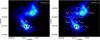 |
Fig. A.1 Spectral map of the o-H2O 212−101 (left panel) and o-H2O 303–212 (right panel) lines overlaid on the PACS continuum emission at 179 μm. The spectra are displayed in the velocity range [–350, 250] km s-1 as line-to-continuum ratio. In the left panel, the red rectangle outlines the region where the CH+ (2–1) line is detected (emission at redshifted velocities compared to the o-H2O 212−101 transition). |
All Tables
Herschel/HIFI observed water line transitions (toward the hot core region in pointing mode).
Observed line emission parameters for the detected lines with HIFI toward G327-0.6 hot core pointed position.
All Figures
|
Fig. 1 Large-scale Spitzer image at 3.6 μm of G327.36–0.6. The boxes show the areas mapped with PACS at 89 and 179 μm (solid white line), with HIFI at 1113 GHz (white dashed line), and at 987 GHz (red line). The white crosses and triangle mark the positions discussed in Paper I. |
| In the text | |
|
Fig. 2 Color scale and white contours are the PACS continuum image of G327.36–0.6 at 89 (top panel, resolution is 9.1″) and 179 μm (bottom panel, resolution is 12.3″). Contours are from 5% of the peak flux in steps of 10%. The triangles mark the positions of the submillimeter continuum peaks reported in Table 3. The red box outlines the area plotted in Fig. 3. |
| In the text | |
|
Fig. 3 Distribution of the SABOCA continuum emission at 350 μm along the infrared dark cloud in G327.3–0.6. Contours are from 5% of the peak flux in steps of 10%. The triangles mark the positions of the submillimeter continuum peaks reported in Table 3. The red cross marks the position observed for the single pointing HIFI observations. The white circle in the bottom left corner shows the beam of the SABOCA observations. |
| In the text | |
|
Fig. 4 Distribution of the continuum emission at 179 μm in G327.3–0.6 (color scale). The solid red contours represent the distribution of the absorption in the 111 → 000 p-H2O line, integrated in the velocity range vLSR = [−55,−37] km s-1 (from –3σ, –4.5 K km s-1, in steps of –3σ). Labels are the peaks of the 450 μm continuum emission from Minier et al. (2009). |
| In the text | |
|
Fig. 5 Spectral HIFI map of the line-to-continuum ratio of the 111 → 000 p-H2O line toward the IRDC region overlaid on the 13CO(6–5) integrated emission (color image). The temperature axis ranges from –1 to 1.5 K, the velocity axis ranges from –65 to –35 km s-1. The 13CO(6–5) data are smoothed to the resolution of the H2O map. The black triangles mark the positions of the peaks of the 450 μm continuum emission. |
| In the text | |
|
Fig. 6 Integrated HIFI intensity map of the p-H2O 202-111 line ([−50,−38 ] km s-1) toward the IRDC region (color image). The black contours show the SABOCA continuum emission at 350 μm from 5% of the peak flux in steps of 10%. The triangles mark the positions of the submillimeter continuum peaks reported in Table 3. Beams of the observations of the p-H2O 202-111 line (white circle) and of the 350 μm continuum (red circle) are shown in the bottom left corner. |
| In the text | |
|
Fig. 7 Integrated intensity map of the p-H2O 202-111 line in the blue- ([−60,−50 ] km s-1, blue contours from 30% of the peak emission in steps of 10%) and redshifted ([−35,−15 ] km s-1, red contours from 30% of the peak emission in steps of 10%) velocity ranges toward the IRDC region. The gray contours represent the integrated intensity of C18O(9–8) ([−48,−42 ] km s-1, from 50% of the peak emission in steps of 10%). The white triangles mark SMM1 and SMM2, the green cross the position observed in the single-pointing HIFI observations (labeled as outflow in Fig. 8.) The dotted lines outline the cuts used to derive the P-V diagrams discussed in Sect. 3.2.1). |
| In the text | |
|
Fig. 8 Top: color scale and contours show the P-V diagram of the CO(6–5) transition computed along a vertical cut passing through the outflow a) and the hot core position b). Bottom: color scale and contours show the P-V diagram of the 202−111 H2O line computed along a vertical cut passing through the outflow c) and the hot core position d). The cut through the outflow position is from |
| In the text | |
|
Fig. 9 Spectra of the 987 GHz water line (bottom panel) and of CO(6–5) (top panel) at the peak of the red-shifted integrated intensity of the 987 GHz transition. The CO(6–5) spectrum is averaged over the 987 GHz beam. |
| In the text | |
|
Fig. 10 (r−v) diagrams of the Hii region G327.3–0.5 obtained from the 12CO(6–5) (left) and from the 111–000-p H2O (right) data cubes. The radius axis is the distance to the shell expansion center, chosen to be the peak of the cm continuum emission. The black solid half-ellipse represents an ideal shell in (r−v) diagram with an expansion velocity of 5 km s-1 centered on –50 km s-1, the dashed white half-ellipse an ideal shell with an expansion velocity of 6.5 km s-1 centered on –45 km s-1. |
| In the text | |
|
Fig. 11 Left: HIFI map of the 111 → 000 p-H2O line toward the Hii region overlaid on the 13CO(6–5) integrated emission (see Paper I). The temperature axis ranges from –1 to 1.5 K. The spectra are continuum subtracted. The 13CO(6–5) data are smoothed to the resolution of the H2O map. The triangle marks the Hii region from Paper I. Right: spectral maps of the 111 → 000 p-H2O line (black) and of the 13CO(10–9) transition (red). In both panels, the velocity axis ranges from –65 to –35 km s-1. |
| In the text | |
|
Fig. 12 HIFI spectra of the H217O/H218O (left) and H216O (right) lines (in black), with continuum for G327.3–0.6 hot core pointed position. The best-fit model with varying (from line to line) and constant (2.6 km s-1) turbulent velocity is shown as a red and dashed blue line above the spectra. Vertical dotted lines indicate the VLSR (–43.2 km s-1 from the line modeling). The spectra have been smoothed to 0.2 km s-1, and the continuum is divided by a factor of two. |
| In the text | |
|
Fig. 13 HIFI spectra of 13CO J = 10–9, C18O J = 9–8, and CS J = 11–10 lines for the HIFI pointed position. The spectra have been smoothed to 0.2 km s-1. The vertical dotted line indicates the source velocity derived from Gaussian fitting, i.e., –44.8 km s-1. |
| In the text | |
|
Fig. 14 Distribution of the equivalent width of the 111 → 000 p−H2O line in the IRDC. The black contours show the SABOCA continuum emission at 350 μm from 5% of the peak flux in steps of 10%. |
| In the text | |
|
Fig. 15 Spectra of p-H218O 111–000 (× 6.2, in red) and p-H217O 111–000 (× 21, in blue) lines overplotted on the p-H2O 111–000 spectrum (in black). The spectra have been smoothed to 0.3 km s-1 (1.4 km s-1 for the H217O spectrum). |
| In the text | |
|
Fig. 16 Spectra of o-H217O 212–101 (× 0.3, in blue) line overplotted on the p-H217O 111–000 spectrum (in red). The spectra have been smoothed to 1.4 km s-1. |
| In the text | |
|
Fig. 17 Spectra of p-H218O 111–000 line (in black) showing the different Gaussian components used to fit the line (red = green+blue+purple). |
| In the text | |
|
Fig. 18 Resulting line profile (in red) of the p-H2O 111–000 line corrected from the absorption shown in green and derived from the p-H218O 111–000 Gaussian line fitting. The original spectra are shown in black. The blue curve is the Gaussian fitting of the outflow. |
| In the text | |
|
Fig. 19 APEX images from Wyrowski et al. (2006) in the N2H+ (3–2) and the CH3OH lines (red and black contours) overlaid on the 8 μm GLIMPSE emission. Embedded GLIMPSE point sources with massive YSO characteristics are marked with triangles. The Herschel 1113 GHz beam is indicated by the white circle centered on the HIFI observed position. |
| In the text | |
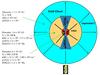 |
Fig. 20 Sketch of the G327 hot core source (arbitrary scale). See details in Sect. 6. |
| In the text | |
|
Fig. A.1 Spectral map of the o-H2O 212−101 (left panel) and o-H2O 303–212 (right panel) lines overlaid on the PACS continuum emission at 179 μm. The spectra are displayed in the velocity range [–350, 250] km s-1 as line-to-continuum ratio. In the left panel, the red rectangle outlines the region where the CH+ (2–1) line is detected (emission at redshifted velocities compared to the o-H2O 212−101 transition). |
| In the text | |
Current usage metrics show cumulative count of Article Views (full-text article views including HTML views, PDF and ePub downloads, according to the available data) and Abstracts Views on Vision4Press platform.
Data correspond to usage on the plateform after 2015. The current usage metrics is available 48-96 hours after online publication and is updated daily on week days.
Initial download of the metrics may take a while.