| Issue |
A&A
Volume 600, April 2017
|
|
|---|---|---|
| Article Number | A82 | |
| Number of page(s) | 20 | |
| Section | Stellar structure and evolution | |
| DOI | https://doi.org/10.1051/0004-6361/201629225 | |
| Published online | 04 April 2017 | |
The VLT-FLAMES Tarantula Survey
XXV. Surface nitrogen abundances of O-type giants and supergiants⋆,⋆⋆
1 Astronomical Institute Anton Pannekoek, Amsterdam University, Science Park 904, 1098 XH, Amsterdam, The Netherlands
e-mail: This email address is being protected from spambots. You need JavaScript enabled to view it.
2 Argelander-Institut für Astronomie, Universität Bonn, Auf dem Hügel 71, 53121 Bonn, Germany
3 UK Astronomy Technology Centre, Royal Observatory Edinburgh, Blackford Hill, Edinburgh, EH9 3HJ, UK
4 Institute of Astrophysics, KU Leuven, Celestijnenlaan 200D, 3001 Leuven, Belgium
5 LMU Munich, Universitätssternwarte, Scheinerstrasse 1, 81679 München, Germany
6 University Vienna, Department of Astrophysics, Türkenschanzstr. 17, 1180 Vienna, Austria
7 Department of Physic and Astronomy, University of Sheffield, Sheffield, S3 7RH, UK
8 Astrophysics Research Centre, School of Mathematics and Physics, Queen’s University of Belfast, Belfast BT7 1NN, UK
9 Departamento de Astrofísica, Universidad de La Laguna, Avda. Astrofísico Francisco Sánchez s/n, 38071 La Laguna, Tenerife, Spain
10 Instituto de Astrofísica de Canarias, C/ Vía Láctea s/n, 38200 La Laguna, Tenerife, Spain
11 European Space Astronomy Centre (ESAC), Camino bajo del Castillo s/n, Urbanizacion Villafranca del Castillo, Villanueva de la Cañada, 28 692 Madrid, Spain
12 Lennard-Jones Laboratories, Keele University, Staffordshire, ST5 5BG, UK
13 Institute of Astronomy with NAO, Bulgarian Academy of Sciences, PO Box 136, 4700 Smoljan, Bulgaria
14 Centro de Astrobiología (CSIC-INTA), Ctra. de Torrejón a Ajalvir km-4, 28850 Torrejón de Ardoz, Madrid, Spain
15 Department of Physics, University of Oxford, Keble Road, Oxford OX1 3RH, UK
16 Armagh Observatory, College Hill, Armagh, BT61 9DG, UK
17 Space Telescope Science Institute, 3700 San Martin Drive, Baltimore, MD 21218, USA
Received: 30 June 2016
Accepted: 12 August 2016
Abstract
Context. Theoretically, rotation-induced chemical mixing in massive stars has far reaching evolutionary consequences, affecting the sequence of morphological phases, lifetimes, nucleosynthesis, and supernova characteristics.
Aims. Using a sample of 72 presumably single O-type giants to supergiants observed in the context of the VLT-FLAMES Tarantula Survey (VFTS), we aim to investigate rotational mixing in evolved core-hydrogen burning stars initially more massive than 15 M⊙ by analysing their surface nitrogen abundances.
Methods. Using stellar and wind properties derived in a previous VFTS study we computed synthetic spectra for a set of up to 21 N ii-v lines in the optical spectral range, using the non-LTE atmosphere code FASTWIND. We constrained the nitrogen abundance by fitting the equivalent widths of relatively strong lines that are sensitive to changes in the abundance of this element. Given the quality of the data, we constrained the nitrogen abundance in 38 cases; for 34 stars only upper limits could be derived, which includes almost all stars rotating at νesini> 200 km s-1.
Results. We analysed the nitrogen abundance as a function of projected rotation rate νesini and confronted it with predictions of rotational mixing. We found a group of N-enhanced slowly-spinning stars that is not in accordance with predictions of rotational mixing in single stars. Among O-type stars with (rotation-corrected) gravities less than log gc = 3.75 this group constitutes 30−40 percent of the population. We found a correlation between nitrogen and helium abundance which is consistent with expectations, suggesting that, whatever the mechanism that brings N to the surface, it displays CNO-processed material. For the rapidly-spinning O-type stars we can only provide upper limits on the nitrogen abundance, which are not in violation with theoretical expectations. Hence, the data cannot be used to test the physics of rotation induced mixing in the regime of high spin rates.
Conclusions. While the surface abundances of 60−70 percent of presumed single O-type giants to supergiants behave in conformity with expectations, at least 30−40 percent of our sample can not be understood in the current framework of rotational mixing for single stars. Even though we have excluded stars showing radial velocity variations, of our sample may have remained contaminated by post-interaction binary products. Hence, it is plausible that effects of binary interaction need to be considered to understand their surface properties. Alternatively, or in conjunction, the effects of magnetic fields or alternative mass-loss recipes may need to be invoked.
Key words: stars: early-type / stars: abundances / stars: rotation / galaxies: star clusters: individual: 30 Doradus / line: profiles / Magellanic Clouds
Based on observations collected at the European Organisation for Astronomical Research in the Southern Hemisphere under ESO programme 182.D-0222.
Tables 2, A.1 and A.2 are available at the CDS via anonymous ftp to cdsarc.u-strasbg.fr (130.79.128.5) or via http://cdsarc.u-strasbg.fr/viz-bin/qcat?J/A+A/600/A82
© ESO, 2017
1. Introduction
Despite the importance of massive stars for Galactic and extragalactic astrophysics, many of the physical processes that control the evolution of these objects are still not well understood (see e.g., Langer 2012). As one of the key agents of massive star evolution, the effects of rotation are manifold. The internal structure of spinning stars becomes latitude dependent (von Zeipel 1924) and centrifugal forces resulting from rotation may lead to deviation results in such stars showing relatively hot and bright polar regions and relatively cool and dim equatorial zones – effects that are actually observed (Domiciano de Souza et al. 2003, 2005). Spinning stars have longer main-sequence lifetimes (Brott et al. 2011a; Ekström et al. 2012; Köhler et al. 2015) and may follow different paths in the Hertzsprung-Russell diagram (HRD), as the centrifugal force reduces the effective gravity and because rotation may also impact mass-loss and angular momentum loss at the surface (see Maeder 2009; Langer 2012, for an extensive discussion).
Rotation induced instabilities trigger internal mixing, transporting material from deep layers to the surface. In extreme cases, this mixing may be so efficient that the stars remain chemically homogeneous throughout their lives and – because of this – avoid envelope expansion (Maeder 1987). In special cases, this type of evolution has been proposed to lead to long-duration gamma ray bursts (e.g., Yoon & Langer 2005; Woosley & Heger 2006). Chemical homogeneity is further a pivotal ingredient for certain formation channels of close-binary black holes, that may over time merge and emit a gravitational wave signal (de Mink et al. 2009; Mandel & de Mink 2016; Marchant et al. 2016).
Helium may, in principle, serve as a tracer of the efficiency of rotationally induced mixing processes. However, as it is produced on the nuclear timescale, the anticipated surface enrichment of He is relatively minor. In this paper we focus on the surface abundance of nitrogen, which is a much more sensitive agent. In the CN (and CNO) cycle, carbon (and oxygen) are converted into nitrogen. Processed material that can escape from the core before a chemical gradient is established at the core boundary, can be mixed into the envelope (Meynet & Maeder 1997). This material will, over time, reach the stellar surface. The faster the star is spinning, the more quickly the material will surface and a greater surface N abundance will be reached.
Hunter et al. (2008) searched for a correlation between surface nitrogen abundance and projected spin velocity of a sample of evolved main-sequence early B-type stars, observed in the context of the VLT-FLAMES Survey of Massive Stars (Evans et al. 2006). A subset of their sample displayed such a correlation and was used by Brott et al. (2011b) to calibrate the efficiency of rotational mixing at the metallicity of the Large Magellanic Cloud (LMC). However, two groups of stars did not concord with the expectations of rotational mixing. We discuss this further in Sect. 6.4, comparing their findings for B stars with ours for O stars. Here, we determine the nitrogen abundance of LMC O-type giants and supergiants that have been observed in the context of the VLT-FLAMES Tarantula Survey (VFTS; Evans et al. 2011). The main questions we want to address are: what is the behaviour of these O-type stars in terms of N-abundance as a function of projected spin velocity? Does our sample also contain groups of stars that are not in agreement with the predictions of rotational mixing in single stars? If so, can these be identified as the counterparts of the peculiar groups identified among the B dwarfs by Hunter et al. (2008)?
The paper is organised as follows. In Sect. 2 we briefly introduce the sample of O giants and supergiants. The method of nitrogen abundance analysis is explained in Sect. 3. The results are presented in Sect. 4, compared to population synthesis predictions in Sect. 5, and discussed in Sect. 6. Finally, we summarise our findings in Sect. 7.
2. Sample and data
The VFTS project and the data have been described in Evans et al. (2011). In short, it is a multi-epoch study of about 800 O- and B stars in the 30 Doradus region of the LMC. The data analysed in this paper were obtained with the Medusa-Giraffe mode of the Fibre Large Array Multi-Element Spectrograph instrument (FLAMES; Pasquini et al. 2002), mounted on the Very Large Telescope (VLT) at Cerro Paranal, Chile. Spectral coverage provided by the adopted settings is λλ 3960−5070 Å and λλ 6442−6817 Å, at spectral resolving powers R ~ 8000 and R ~ 16 000, respectively; full details are given by Evans et al. (2011).
Multi-epoch observations allowed for a selection of spectroscopic binaries on the basis of their radial velocity (RV) variation (Sana et al. 2013). We consider that stars are spectroscopically single if their peak-to-peak RV variation is either statistically insignificant or significant but smaller than 20 kms-1. About half of the stars in the latter category are however genuine spectroscopic binaries (Almeida et al. 2017; see also Sect. 3.4). Spectral classification of the O-type content has been presented by Walborn et al. (2014). Here we analyse the nitrogen content of the presumably single O-type stars classified by Walborn et al. (2014) as giants, bright giants and supergiants. An overview of the distribution of our sample stars among luminosity classes III to I is given in Table 3. These luminosity classes could be assigned in 72 cases. For 31 stars no luminosity class identifier could be given. We provide estimates for their nitrogen abundance in Appendix A.2.
3. Method
3.1. Atmospheric parameters
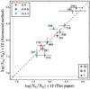 |
Fig. 1 Comparison between nitrogen abundances derived with the automated fitting method (vertical axis) and the method described in Sect. 3 (horizontal axis). Dotted lines indicate the nitrogen baseline abundance of LMC stars. The dashed line shows the 1:1 relation. The observed stars are marked with their VFTS ID. Except for two stars the two methods agree within 1σ. Note that ξm is allowed to vary in the automated method, while ξm is fixed at 10 kms-1 for the measurements in this paper (see Sect. 3.4). |
Atmospheric properties of the sample discussed here have been determined by Ramírez-Agudelo et al. (2017), using an automated fitting method (Mokiem et al. 2005; Tramper et al. 2011, 2014). In short, the method combines an analysis of normalised spectra using the non-LTE stellar atmosphere model FASTWIND1 (Puls et al. 2005) with the genetic fitting algorithm pikaia (Charbonneau 1995). FASTWIND accounts for a trans-sonic, stationary, radial stellar outflow. Six stellar properties have been determined: effective temperature Teff, surface gravity g, (unclumped) mass-loss rate Ṁ, helium content NHe, a depth-independent micro-turbulent velocity ξm, and projected equatorial rotational velocity νesini. The luminosity L and radius R of the star were constrained using the self-consistently computed KS bolometric corrections and the Stefan-Boltzmann law. The stellar wind was assumed to accelerate following a β-type velocity law, which is prescribed by the flow acceleration parameter β and the terminal flow velocity ν∞. Appropriate values for β are adopted from hydrodynamical simulations (Muijres et al. 2012); values for ν∞ follow from a scaling relation with the surface escape velocity (Kudritzki & Puls 2000; Leitherer et al. 1992).
For relatively hot stars, an accurate estimate of the effective temperature from H and He lines only is severely compromised when the He i lines disappear from the spectrum; for relatively cool stars when He ii fades away. Because of this, Ramírez-Agudelo et al. (2017) have added nitrogen to their set of hydrogen and helium diagnostic lines for a total of 11 stars (see Fig. 1). The inclusion of nitrogen not only enables better constraints on Teff, based on the corresponding ionisation equilibrium, but also allows to derive nitrogen abundances in parallel. As will be discussed in Sect. 3.3, we adopt an alternative, faster method to determine the nitrogen fraction of all stars in our sample. In Fig. 1, we compare the nitrogen abundance determined by the automated method with our own measurements for the 11 sources mentioned. Save for two sources that deviate by two sigma, both methods agree within one standard deviation. This level of compatibility is in agreement with statistical fluctuations, that are expected for independent measurements in a sample of 11 sources. For the sake of consistency, we adopt the abundances as measured by the method presented in Sect. 3.3 throughout this work.
3.2. Nitrogen diagnostic lines
The physics of nitrogen line-formation and its implementation into FASTWIND have been extensively described and tested by Rivero González et al. (2011, 2012a,b). Here we discuss the diagnostic lines used in the work at hand.
In the optical spectral range available to us (covering λλ 3960−5070 Å and λλ 6442−6817 Å) several tens of nitrogen lines can be identified. Not all of these lines are suited for spectral analysis. To select the lines that are most suitable for our purposes we applied the following selection criteria: (i) the lines should not be blended; (ii) the lines should be strong enough to be detectable given the typical signal-to-noise (S/N) of our spectra and the range of projected spin velocities covered by our stars; (iii) the line strengths should be as sensitive as possible to changes in abundance. To assess the latter we computed a grid of FASTWIND models, covering the range of spectral types and luminosity classes, in which we varied the nitrogen abundance relative to hydrogen  (1)where NN and NH are the number abundances of nitrogen and hydrogen. We vary εN from εN = 6.93, which is close to the LMC baseline value (Kurt & Dufour 1998), to εN = 8.53. Figure 2 shows the outcome of this test for a few representative spectral lines. As expected, most lines only show sensitivity in a given temperature range. On the basis of this exercise we compiled a list of primary and secondary diagnostic lines, which is given in Table 1. Primary lines are those most often used for abundance measurements, as they show reliable results. Secondary lines are often not visible or may give anomalous results as explained in the next paragraphs.
Diagnostic lines used to derive the nitrogen abundance.
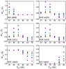 |
Fig. 2 Equivalent width as a function of effective temperature and nitrogen abundance for several diagnostic lines. Colours, following the rainbow from red to purple, indicate nitrogen abundances εN ranging from 6.93 to 8.53 in steps of 0.4 dex. Negative values of Weq represent emission. For all models: log g = 3.9 (cgs), log Ṁ = −6 (M⊙/ yr) and ξm = 7 kms-1. |
The N iii λ4634−4640−4641 triplet in emission, in combination with He ii λ4686, is used to assign O-type stars the qualifier f (Sota et al. 2011). The modelling of this triplet is complex and has been described in detail by Rivero González et al. (2011). We confirm their findings that the abundances derived from this triplet are sometimes anomalous compared to that of other lines and therefore we use it as a secondary diagnostic.
One of the strongest lines, N iii λ4097, is situated in the wing of Hδ. To perform an equivalent width analysis, we divided the observed profile by a fit to the Hδ wing as if it represented the continuum. In some cases this method worked, however in other cases anomalous abundances (with respect to constraints from other lines) were found. In particular, we found for 15 stars that the N iii λ4097 profile is underpredicted when adopting the N-value derived from other lines. We thus used this line too as a secondary diagnostic only.
As stars rotate faster and their lines become broader, neighbouring spectral lines can blend with each other. This is in particular the case for the N iii λ4511−4515−4518 complex. In these cases we attempted to extract the combined Weq from the spectrum (see Sect. 3.3). Unfortunately, the S/N of our data is such that for almost all rapidly rotating (νesini~> 170 kms-1) stars in our sample, the spectral lines could not be distinguished from the noise.
Rivero González et al. (2012b) derived the nitrogen abundances of LMC O-type stars relying mostly on the same lines that we use. Martins et al. (2015a), studying Galactic stars using the code cmfgen (Hillier & Miller 1998), rely on 4 to 22 lines that partly overlap with our set of lines. By virtue of their wider spectral range and higher baseline abundance, Martins et al. were able to use more, as well as intrinsically weaker, spectral lines. However, their list does not include our primary lines N iii λ4379, N iv λ4058 and N v λ4603−4619.
It is noteworthy that the only N iv line available to us (4058 Å) is also sensitive to effects other than variation of the nitrogen abundance, as described by Rivero González et al. (2012a,b). Unfortunately N iv λ6380, a spectral line that is known to be strong (e.g., Rivero González et al. 2012b), lies outside of our spectral range.
3.3. Abundance determination
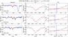 |
Fig. 3 Abundance measurement for VFTS 466, a relatively high S/N source. Not all lines used are shown. Left panels: the observed spectrum is shown in blue and the best model fit in black. The nitrogen abundance of the best model resulted from combining all utilised lines and is given by the εN in the figure title. The selection of the fit region is displayed in red. Middle panels: zoom in on the fitted region, with the best fit Gaussian profile in red. Right panels: theoretical Weq values as a function of εN (horizontal axis) are shown in black. Measured Weq and interpolated εN are in red and blue, respectively. Dashed red lines indicate the measurement error and dashed blue lines the corresponding uncertainty in the best fit value. |
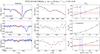 |
Fig. 4 Same as Fig. 3, for VFTS 103, typical for relatively low S/N. In the case of the N iii λ4379 line (middle row), no Gaussian profile could be fitted. However, the final line profile that is derived from measurements to other lines, is consistent with the data. |
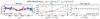 |
Fig. 5 Example of a Weq measurement by integration (for VFTS 399). The Weq is extracted by integration of the red region of the spectrum in the left panel. In the middle panel, this is compared to theoretical Weq values of the combined complex as predicted by FASTWIND, yielding εN and its associated error. The robustness of the measurement is checked twofold: first by comparing a model with the final solution to the observed spectrum (left panel, solid black line). Second, in the right panel, by comparing the abundance measurements that result from adjustment of the integration bounds, varying the width Δλ as function of the adopted width Δλ0, where the adopted measurement is indicated by the red triangle. The 1σ error on Weq is calculated through propagation of the error spectrum. |
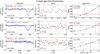 |
Fig. 6 VFTS 711, 080, and 109 are examples of cases for which only upper limits could be derived. Left panels: the observed spectrum is shown in blue, the region used to determine the S/N in red, and the model representing the upper limit in black. Middle panels: zoom in on the fitted region. For these cases this region is used to determine the S/N. The red line is the mean flux level of this range; the dashed lines indicate the standard deviation. Right panels: theoretical depth values as a function of εN in black, where the minimal detectable depth and its inferred upper limit are indicated as the red horizontal and the blue vertical line respectively. The resulting upper limit is indicated in the top left corner of the right panel. The line depression for the upper limit to εN can be considerably larger than the noise would suggest as a result of our conservative choice for this limit (see Sect. 3.3). |
We measured the equivalent width Weq of our lines by fitting a Gaussian to their continuum normalised profiles (see the middle columns of Figs. 3 and 4). In this procedure, the continuum was held fixed. The centre of the line was allowed to vary within the uncertainty of the RV measurement. The (weak) nitrogen lines are well represented by a Gaussian profile, the fitting of which provides a straightforward way of extracting Weq and its associated error, given the quality of the data.
Next, using the stellar properties given by Ramírez-Agudelo et al. (2017), we computed a set of five FASTWIND models for each star, in which we varied the nitrogen abundance from the baseline value εN = 6.93 to εN = 8.53 in steps of 0.4 dex. This covers the full range of measured εN. The behaviour of the line strength as a function of εN can be accurately represented on the basis of these points using a second order polynomial, as is shown in the right-most panels of Figs. 3 and 4. For each spectral line, the N-abundance and its error (blue solid and dashed lines) was then extracted on the basis of the measured Weq and its error (red solid and dashed lines). For each star, we combined the results from the different lines that were visible in the spectrum. We computed a weighted mean, where the N-abundance measured from each line i was weighted according to its error as  . We considered the weighted standard deviation to be the error on the measurement of εN. Independently, the error on the weighted mean can be calculated through propagation of the error on the measurements from individual lines. In cases where the error on the weighted mean was larger than the weighted standard deviation, we adopted the former as error of the measurement.
These errors do not take into account uncertainties in the determined stellar parameters and in the placement of the continuum. To test the impact of the former on our abundance measurements we computed models ranging over the 2σ errors provided by Ramírez-Agudelo et al. (2017). We did this for three stars, representative for late, mid and early spectral type, and for the three parameters that impact our measurement the most, Teff, g and Ṁ. For each permutation of the lower and upper errors in the parameters, we repeated our nitrogen abundance measurement. In these measurements, we observed a peak-to-peak spread in εN of typically ~0.4 dex, extending up to 0.6 dex in the case of the hottest star, where the uncertainty in Ṁ is dominant2. We conclude that the 2σ uncertainties in the atmospheric parameters induce an error that may reach up to ~0.2−0.3 dex in extreme cases; hence the 1σ uncertainty may reach half of this value. The uncertainty in the location of the continuum is an additional source of error in the Weq determination. Sana et al. (2013) reported that the continuum is constrained to better than 1% on average. We estimate the corresponding error in the determination of εN to be up to 0.15 dex for modestly rotating stars. In the course of this work, we will consider the error on our abundance measurements to be the standard deviation of the N-abundance that is measured from different diagnostic lines.
Figures 3 and 4 show two examples of the Weq analysis, for VFTS 466 and VFTS 103, typical for high and low S/N data respectively. In each case, results for only a few of the fitted lines are shown. In the right hand columns, the quadratic interpolation of the observed Weq (red horizontal line) with the theoretical Weq (black dots and line) is shown. By computing a model with the final solution, and overplotting it on the data, we test the robustness of the method (left columns of Figs. 3 and 4).
In some cases a measurement of Weq could not be extracted from the spectrum through fitting a Gaussian profile (e.g., due to blending with neighbouring lines). In these cases we obtained Weq by direct integration of the spectrum. One example, for VFTS 399, is shown in Fig. 5. Keeping the continuum fixed, we integrated the spectral range where the N-lines are predicted to reside (red range in the left panel) and calculated the error on Weq by propagation of the error spectrum. By comparing the observed Weq with the theoretical values from FASTWIND, we extracted a εN measurement and its error (middle panel). By overplotting a model with the final solution on the data (left panel) and comparing the resulting measurements of different integration ranges (right panel), we tested the robustness of the method. This method was employed for the N iii λ4511−4515−4518 complex in 4 cases, namely VFTS 185, 399, 513, 569. For VFTS 399, good agreement is found with earlier findings by Clark et al. (2015), who performed a by-eye comparison, confirming the N-enriched nature of the star.
Table 2 (only available at the CDS) records, for all stars that have their N-abundance determined, the measured Weq and associated uncertainty per diagnostic line. Values are given if the respective line was included in the analysis. Figure C.1 shows additional examples of line fits, for stars across the full range of considered spectral types and N ionisation stages. It shows that, in order to reproduce the N line profiles of these sources, significant surface enrichment is required.
If no lines are detected, an upper limit on εN can be set. Examples of this are shown in Fig. 6. From the calculated models the strongest spectral lines in terms of depth were selected. For these lines the noise in the continuum was measured and converted into a minimal detectable depth, given by 2 × σcont. In doing so, we assumed the line is detectable when its depth constitutes twice the noise level. The predicted depth as a function of εN was measured from the models and again described by a quadratic fit. For each line, the minimal detectable depth then yielded the upper limit on εN. The resulting upper limit is thus solely based on the (predicted) depth of a line, rather than its Weq. Assessing the outcome of this method for the strongest 5−7 lines, taking into account their local continuum noise and individual strengths, allowed us to set an upper limit on the nitrogen abundance of a star. We pursued to use the nitrogen line that sets the tightest constraint on εN. If we adopted a 1σ (instead of the 2σ) criterion, resulting upper limits are lower by about 0.4 dex.
3.4. Limitations of the method
Though the nitrogen lines appear weak, they may suffer from saturation effects and therefore their strength can be a function of the micro-turbulent velocity. The ξm values, fitted by Ramírez-Agudelo et al. (2017), range between a few and 30 kms-1, often with sizable uncertainties, and where 30 kms-1 is the fixed upper boundary considered by these authors. We investigated the effect of the micro-scale turbulent motions on the nitrogen abundance by computing new FASTWIND models with the same atmospheric parameters, but adopting a fixed ξm of 10 kms-1. Following the method described in Sect. 3.3 we derived the N-abundance also for this constant value. Since the Weq of a line is in principle a positive function of ξm, one expects measurements to yield lower εN when fitted with a higher ξm (keeping all other parameters fixed). However, the micro-turbulence may also affect the atmospheric structure and thus the emergent line profiles. In Fig. 7 we show the difference in εN between the two methods as a function of the ξm value from the automated fitting approach. The differences are typically less than 0.2 dex. Because the ξm values are largely unconstrained, i.e. have large uncertainties, by Ramírez-Agudelo et al. (2017), we henceforth adopt ξm = 10 kms-1 in all our computations.
Ramírez-Agudelo et al. (2017) determined the atmospheric parameters without taking into account macro-turbulent broadening of spectral lines. This leads to νesini values that in the regime up to ~150 kms-1 are, on average, somewhat larger than those incorporating macro-turbulent broadening (see Ramírez-Agudelo et al. 2013; Simón-Díaz & Herrero 2014; Markova et al. 2014, for a discussion). We too neglected macro-turbulent broadening and adopt νesini values given by Ramírez-Agudelo et al. (2017). Since rotation and macro-turbulent motions conserve equivalent width, this has a marginal impact on our measurements of the N-abundance.
In the spectra of some rapidly rotating stars, we saw signs of the N iii λ4097 line. However, due to the severe broadening, we could not extract Weq through a combined Gaussian and Lorentzian fit (the Lorentzian fit was employed to represent the wing of Hδ, hence the local continuum of the N iii line; see Sect. 3.2). In these cases, spectral synthesis would be the better option. However, we found this line often to be underpredicted in cases where other lines provide independent measurements (see Sect. 3.2). The εN required to reproduce the N iii λ4097 line would imply that other diagnostic lines should be visible. We thus opted in these cases for an upper limit that brings the predicted FASTWIND profiles in agreement with the observed profile of N iii λ4097, but would yield other visible diagnostic lines.
Our sample contains 6 stars which were, after radial velocity measurements at additional epochs, identified as long-period spectroscopic binaries (Almeida et al. 2017). These stars are VFTS 064, 093, 171, 332, 333, 440. Since their spectra are fitted assuming they were single, their resulting parameters should be considered with caution. As such they are excluded from the quantitative comparison with theory in Sect. 5.2. VFTS 399 is excluded in that section as well, since it may be an X-ray binary (Clark et al. 2015). The abundance measurements of these 7 stars are flagged in Fig. 8. In the sample of stars with no luminosity class identifier, Ramírez-Agudelo et al. (2017) find no satisfactory fit to the spectral lines of another 6 objects. Finally, we are unable to reliably extract the nitrogen abundance of one source (VFTS 177, see also Appendix A.2). These further 7 objects are also excluded from the analysis in Sect. 5.2.
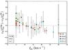 |
Fig. 7 Difference in the measured N-abundance using the micro-turbulent velocity as determined by Ramírez-Agudelo et al. (2017) and ξm = 10 kms-1. All stars for which the nitrogen abundance could be determined are shown. |
4. Results
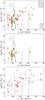 |
Fig. 8 Nitrogen abundance versus projected rotational velocity. For all panels, symbols denote luminosity class and colours spectral type; see legend in the top panel. Top panel: entire sample. The newly detected binaries have a yellow circle underlaid (see Sect. 3.4). Middle panel: subset of stars for which the nitrogen abundance could be measured. Bottom panel: subset of stars for which only upper limits could be derived. The dashed lines indicate detection limits for different S/N and are discussed in Sect. 4. The black solid lines are evolutionary tracks for the O-type stage (Teff ≥ 29 kK) of a 20 M⊙ star (Brott et al. 2011a), with initial rotational velocities of 114, 170, 282 and 390 kms-1. We multiply the rotational velocity of these tracks by π/ 4 to account for the average projection effect. |
Number of stars for which the nitrogen abundance could be constrained and for which only upper limits could be derived, as a function of luminosity class.
The derived surface nitrogen abundances and their uncertainties are listed in Table A.1. In Fig. 8 they are plotted as function of the projected rotational velocity. Note that these values of νesini are, strictly, upper limits, due to the neglect of macro-turbulent broadening. The symbol type denotes the luminosity class. Of the 72 sources studied, we constrained εN in 38 cases and had to settle for upper limits in 34 cases; see also Table 3. The 7 newly detected binaries in the sample are identified by a yellow circle (see Sect. 3.4).
Also shown are evolutionary sequences by Brott et al. (2011a) for a 20 M⊙ star during its O-type phase (Teff ≥ 29 kK). The surface rotational velocity of the tracks from Brott et al. is essentially constant during its main-sequence evolution. This is the result of a competition between angular momentum transport from the core to the envelope, and envelope expansion.
Except for VFTS 399, the sources for which the nitrogen abundance could be determined have νesini up to 170 kms-1. They span a fairly wide range of εN values, from about 7.0 to 8.8, and are shown separately in the middle panel of Fig. 8. Stars with εN~> 8.1 are predominantly early-type stars. Also, the supergiants are all quite enriched having εN~> 7.7.
For all but one star spinning faster than 170 kms-1 we could only derive upper limits. These are essentially set by the signal-to-noise ratio of the spectrum and νesini. This is illustrated in the bottom panel of Fig. 8. The dashed lines show detection limits covering the range of S/N of our sample stars. They have been computed for a star of spectral type O9, representing the bulk of our sample, by considering the primary diagnostic line N iii λ4379. For each S/N we established the minimum detectable depth from the inverse of the S/N, for a range of νesini. For each νesini, we compared the minimal detectable depth to model spectra for a range of εN values (at the appropriate νesini). This procedure yielded the detection limits drawn in the panel. Given that the typical S/N of our data is ~100−200, one may indeed have anticipated difficulties in constraining the nitrogen abundance at νesini> 200 kms-1.
5. Comparison to population synthesis
In this section we compare our findings to the nitrogen enrichment pattern that is expected for a comparable (synthetic) population of single O-type stars. This allows us to test models of stellar evolution in the initial mass range of 15 M⊙ and up, specifically the treatment of rotation induced mixing. We limited this test to models by Brott et al. (2011a), as these cover a wide range of initial spin rates and have initial CNO abundances that are tailored to the LMC environment.
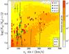 |
Fig. 9 Nitrogen abundance versus projected rotational velocity for the full sample. Symbols indicate luminosity class, colours indicate spectral subtype. Tracks (Brott et al. 2011a) drawn in solid black lines are for a 20 M⊙ star, evolved until the effective temperature is below 29 kK and they become B-type stars. Initial rotational velocities for the tracks are 114, 170, 282 and 390 kms-1 and have been multiplied by π/ 4 to account for the average projection effect. The population synthesis calculation projected in the background is for the O star phase only and assumes a flat distribution of rotational velocities. Out of 740 × 103 simulated stars, 310 × 103 pass the selection criterion (Teff ≥ 29 kK). These are normalised to 72 stars, matching the number of observed stars in the plot. |
5.1. Population synthesis model
Figure 9 again shows the projected spin velocity versus nitrogen abundance for all stars in our sample, with symbol shapes and colours as in Fig. 8. In the background we show the results of a population synthesis computation for O-type stars, based on models by Brott et al. (2011a). These computations were done in the following way. We randomly drew a population of single stars from the evolutionary sequences of Brott et al. (2011a), sampling distribution functions for their initial mass, spin rate and spin axis orientation, and adopting continuous star formation for 15 Myr. Masses follow a Salpeter (1955) initial mass function (IMF) from 10 M⊙ to 60 M⊙. After sampling the IMF, the selected mass was rounded off to the mass of the nearest available evolutionary track3. The initial rotational velocity and age were interpolated between tracks. We assumed the spin axes to be randomly distributed in 3D space.
The initial rotational velocity distribution used to construct Fig. 9 is flat and ranges from 0 kms-1 to 600 kms-1, to clearly illustrate the effect of rotational mixing as a function of the projected spin rate. In later figures, we will use the empirical rotational velocity distribution for single O-type stars derived by Ramírez-Agudelo et al. (2013) as input.
By accepting a drawn star only if its effective temperature is at least 29 kK, we constructed a probability distribution for O-type stars only. After the star was drawn, we imposed Gaussian distributed uncertainties of 0.15 dex in εN and 20% in the rotational velocity, characteristic of the typical empirical errors. Drawn stars with νesini< 40 kms-1 were artificially placed at 40 kms-1, as their spin rates are below the resolution limit of the survey. The results were then grouped in 10 kms-1 × 0.05 dex bins to generate the plot. Finally, the outcome of the simulation was normalised such that the simulated star count integrated over the plot equals the number of observed stars in the figure. Due to the measurement errors imposed on the simulated values, occasionally stars will acquire a nitrogen abundance smaller than 6.8. As the minimum N-abundance that we display in the plots is 6.8, i.e., 0.1 dex below the adopted initial nitrogen abundance for the LMC, we decided to redistribute simulated points with εN< 6.8 to the range [6.8, 7.0] to also visually display the proper normalisation.
The overall predicted trend in Fig. 9 is one of increasing εN with increasing νesini. The reason for the relative dearth of nitrogen normal rapidly rotating stars is that the rate of nitrogen enrichment as a function of the fraction of the main-sequence lifetime is a rather strong function of initial mass: the higher Minit the faster the nitrogen enrichment occurs (Brott et al. 2011b; Köhler et al. 2012). For example, a 10 M⊙ star having an initial rotational velocity of ~225 kms-1 reaches halfway along its main-sequence a nitrogen enrichment that is ~40% of its final main-sequence enrichment. For a 30 M⊙ star halfway along its main-sequence evolution this is already ~85%. This implies that for early-B type stars the lower right corner of the diagram is expected to be more frequently populated than for O-type stars.
5.2. Population synthesis for the O III-I sample
Figure 9 does not allow for a direct comparison between our observations and theory because the adopted (flat) spin distribution is not the observed one, and our sample of O-type stars is for giants to supergiants only, i.e., it lacks O-dwarfs. To facilitate a quantitative assessment, we limited ourselves to the stars that have surface gravities corrected for rotation of log gc ≤ 3.75, for observed as well as simulated stars (see Repolust et al. 2004, for a discussion on the centrifugal correction). The criterion was chosen as a balance between including as many O giants as possible, while excluding as many O dwarfs as possible. In pursuit of completeness, we supplement these O giants with presumed single O stars that have no luminosity class identifier (see Appendix A.2).
In the VFTS sample of presumed single O-dwarfs, analysed by Sabín-Sanjulián et al. (2014), only three sources have surface gravities below this limit. These are VFTS 419, 484 and 581. Preliminary analysis (Símon-Díaz, priv. comm.) shows that these stars spin relatively slowly, 145, 120 and 70 kms-1, respectively, and show modest surface enrichments, εN~ 7.2. These three dwarfs are not included in the following sections. We also do not include the seven binaries and seven sources with no luminosity class identifier that are rated as poor quality fit (see Sect. 3.4).
The total sample of stars with log gc ≤ 3.75 comprises 27 stars (21 O III-I and 6 without an assigned luminosity class). The restriction to lower gravities overall selects the somewhat evolved stars, for which our sample is near to complete within the VFTS. Figure 10 illustrates this by showing the location of these low gravity sources in the HRD relative to other O-type stars in the VFTS, using a colour coding to indicate their N-abundance. The gravity criterion also excludes the late O stars (M ≈ 15 M⊙) that present an ambiguity between the two luminosity class criteria discriminating giants from dwarfs (see Walborn et al.2014; Ramírez-Agudelo et al. 2017, for a discussion).
Figure 11 shows the subset of low gravity sources (excluding the three O dwarfs) together with a population synthesis prediction suitable for direct comparison, i.e., for stars of which the initial spin distribution is as given by Ramírez-Agudelo et al. (2013), that have temperature Teff ≥ 29 kK and gravity log g ≤ 3.75. The population synthesis calculation is normalised as to produce the number of observed stars (27) if integrated over the predicted range of εN and spin rates.
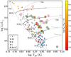 |
Fig. 10 Hertzsprung-Russell Diagram (HRD) for the O-type stars in the VFTS sample, excluding binaries and poor quality fits (Sect. 3.4). Luminosities and temperatures are from Ramírez-Agudelo et al. (2017). Evolutionary sequences and isochrones are from Brott et al. (2011a) and Köhler et al. (2015). The solid tracks alter to dotted tracks for Teff ≤ 29 kK. Grey crosses indicate LC V VFTS stars (Sabín-Sanjulián et al. 2014). The remaining stars are colour-coded according to εN, where upper limits are indicated in blue. Encircled stars have log gc ≤ 3.75, where pink circles indicate that they occupy Box 2 and green circles that they are outside of that box (see Sect. 5.2 and Fig. 11). |
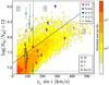 |
Fig. 11 Nitrogen abundance versus projected rotational velocity for 27 O-type stars with gravities log gc ≤ 3.75. It constitutes all of the VFTS sources fulfilling these criteria, save for three O-dwarfs studied by Sabín-Sanjulián et al. (2014) that would all end up in Box 3 (Símon-Díaz, priv. comm.), binaries and poor quality fits (Sect. 3.4). Identical selection criteria have been applied to the population synthesis calculation projected on the background. The applied initial spin distribution in this calculation is assumed to be that derived for the presumed-single VFTS stars (Ramírez-Agudelo et al. 2013). Out of the 721 × 103 simulated stars, 21 × 103 pass the selection criteria (Teff ≥ 29 kK and log gc ≤ 3.75). These are normalised to 27 stars, matching the number of observed stars in the plot. The boxes, separated by the solid black lines, are defined in Sect. 5.2. |
Following Brott et al. (2011b), in Fig. 11 we define boxes in which we count the number of observed and predicted stars. For the sake of clarity, the numbering of these boxes is chosen such as to best correspond to the box-definitions used in that paper:
-
Box 2:
selects the N-enriched stars withνesini< 140 kms-1.
-
Box 3:
comprises the zone where the effects of rotational mixing are expected to be the most pronounced. Stars in this region in principle behave in conformity with theory if the bulk is positioned on or near the predicted coloured diagonal.
-
Box 4:
is a region where neither stars are observed, nor a significant number of them is predicted.
The diagonal separating Boxes 2 and 4 from Box 3 is described by εN = 0.0036 νesini + 7.15. This division is chosen to follow the dark orange diagonal in Figs. 9 and 11, i.e., to encompass the bulk of the simulated rotationally-mixed stars. Brott et al. (2011b) define Box 1 to select non-enriched rapidly-rotating stars (the lower right of Fig. 11), for which our data do not permit firm conclusions.
Table 4 shows the counts of the observed and simulated stars in the different boxes. In the process of counting we took a Gaussian distributed uncertainty in the observed nitrogen abundance into account. Upper limits were uniformly distributed between boxes, considering the distance between their value and εN = 6.8. This can result in a non-integer number of stars occupying a certain box in Table 4.
We found 60 ± 10% of the sample to be in Box 3, containing relatively slowly spinning stars that have at most marginally enhanced nitrogen abundances and stars for which only upper limits to εN could be constrained. Theory predicts 85% of the stars to be in this regime, which appears in reasonable agreement. However, if future measurements with higher S/N data show that all upper limits in this box were close to the LMC baseline abundance, this would be inconsistent with theoretical predictions. As we cannot investigate this with the data at hand, we conclude that this population is not in violation with the predictions of rotational mixing.
Box 2 contains a population of apparently slowly spinning but nitrogen enhanced stars (in Fig. 10 these sources have been given a pink circle around their symbol). While theory predicts 8% of the stars to be in this region, we found 38 ± 9% of the population to be in this box. This amounts to almost 5 times more observed sources than predicted sources. It is unlikely that this large overabundance of observed sources can be explained by statistical fluctuations in the spin axis orientation distribution of these stars, assumed to be random in 3D space. This statement gains more weight by the fact that Box 4 is essentially empty, while population synthesis predicts an equal amount of sources to reside in this region as in Box 2. We conclude that the bulk of the sources in Box 2 are truly slow rotators and that their high nitrogen abundance is not explained by the evolutionary models of Brott et al. (2011a, see also Sect. 6.2).
6. Discussion
In this section we discuss the nature of the stars in Box 2 that do not concur with predictions of rotational mixing in massive stars. We also compare our finding to previous studies. We start by examining the current mass of the stars in our sample.
6.1. Current evolutionary masses
Current evolutionary masses of the stars in our sample have been determined by Ramírez-Agudelo et al. (2017) using Bonnsai4, a Bayesian method to constrain the evolutionary state of stars (Schneider et al. 2014). As independent prior functions these authors adopt a Salpeter (1955) initial mass function, an initial rotational velocity distribution as given by Ramírez-Agudelo et al. (2013), a random orientiation of spin axes, and a uniform age distribution. The observables on which the mass estimates are based are L, Teff and νesini.
Figure 12 presents a summary of the mass properties of the low gravity stars in Fig. 11, comparing the stars in Box 2 to the rest of the sample. Two types of statistics are provided, one based on median statistics (Tuley’s five-number summary) and one based on the mean of the sub-samples. Each of these shows that the objects in Box 2 are appreciably more massive than the remainder of the stars: the median evolutionary mass of stars in Box 2 is 34.8 M⊙, while that of the remaining stars is 25.8 M⊙.
Brott et al. (2011b) performed a similar analysis as done here for a sample of 107 main-sequence B-type stars in the LMC with projected spin rates up to ~300 km s-1 discussed by Hunter et al. (2008, 2009). They too note that the nitrogen enhanced slowly spinning stars appear to have higher masses. Though the bulk of their sample has a mass ≤12 M⊙ the stars that populate Box 2 almost all have masses in between 12−20 M⊙. Further on in this section we discuss scenarios regarding the nature of the Box 2 stars that may explain this behaviour.
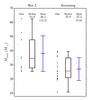 |
Fig. 12 Distribution of evolutionary masses for the stars in Fig. 11 that occupy Box 2 (left) and the remainder of stars (right). Black crosses indicate data points. The middle column in each half of the diagram shows the median of the sample in red, where the boxplot indicates the 0.25 and 0.75 percentiles with whiskers extending out no further than 1.5 times the inter-quartile range. The right column indicates the weighted average and standard deviation (in parentheses) of the sample in blue. Evolutionary masses are calculated using the Bonnsai tool (Sect. 6.1). |
6.2. Current surface nitrogen abundances as predicted by single star evolutionary tracks
In addition to the posterior probability distribution of the current mass, Bonnsai also provides the distribution for the current surface nitrogen abundance. For all but one of the stars for which our analysis resulted in upper limits on εN only, the upper limit is in agreement with the εN predicted by Bonnsai. Out of the 38 stars for which we have a direct εN measurement, only 7 agree within 1σ with the nitrogen abundance expected from their evolutionary state. Interestingly, among these are three binaries (namely VFTS 333, 399 and 440). In the other 31 cases our nitrogen measurement is higher than that predicted by Bonnsai. Since all direct measurements have low νesini, this is an alternative way of expressing that the bulk of our nitrogen rich, slowly rotating sources are not expected from the evolutionary sequences by Brott et al. (2011a).
We repeated the Bonnsai analysis for the 9 sources in Fig. 11 that have measured abundances and occupy Box 2. In this run, we added the measured surface abundances of helium and nitrogen to the observables Teff, L, and νesini. While in the analysis without these extra two observables Bonnsai returned in all cases a modestly rotating star with most probable inclination sin i~ > 0.8, the new run produced fast rotators seen almost pole-on (sini~ < 0.5) in 8 out of 9 cases. This reflects that in order to reproduce the high He- and N-abundances in the tracks of Brott et al. (2011a) more mixing is required, demanding more rapid rotation. Assuming inclinations randomly distributed in 3D space, the probability that out of the 27 stars with log gc ≤ 3.75, 8 have sini ≤ 0.5 is 0.015 5. This too demonstrates that the stars in Box 2 cannot be straightforwardly understood in the context of current single-star evolutionary tracks.
6.3. Correlation between nitrogen and helium abundance
In Fig. 13, we plot the nitrogen surface abundance derived here versus the helium surface fraction (by mass) as derived by Ramírez-Agudelo et al. (2017). Shown in the background is the same population synthesis calculation as discussed in Sect. 5.2 and shown in Fig. 11, i.e., for O-type sources that have log g ≤ 3.75. The results are grouped in bins of 0.01 (Y) × 0.05 (εN) dex. Simulated stars that are helium- as well as nitrogen enriched are all rotating initially at  350 kms-1.
Though the scatter is sizable, the N- and He-abundances of the stars in our sample appear correlated. Such a correlation is also found by Rivero González et al. (2012b). Moreover, the trend agrees quite well with the models, even though the number of predicted and observed stars with He, as well as N, enrichment do not agree. This suggests that though the mechanism that brings N and He to the surface may still be unidentified, it is one that brings a mixture of gases to (or deposits a mixture of gases on) the surface that has the He/N abundance ratio that is expected from the CNO process.
If the exposed material is CNO-processed, an enhancement in N is expected to be accompanied by a depletion of C. An independent verification would thus be to simultaneously measure the surface C abundances of these stars. It should also be noted that several other surface-enrichment mechanisms (e.g., those discussed in Sect. 6.5) are expected to result in the display of CNO-processed material at the surface.
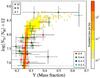 |
Fig. 13 Nitrogen abundance versus surface helium mass fraction. In the background the outcome of population synthesis is projected, as explained in Sect. 5 and shown in Fig. 11. |
6.4. Comparison to other εN−νe sin i studies
We limit a comparison to other studies to main sequence OB stars in the LMC, notably to the work on early-B stars by Hunter et al. (2008, 2009) and Brott et al. (2011b), and on O-type stars by Rivero González et al. (2012b). For an analysis of LMC B-type supergiants see Hunter et al. (2008) and McEvoy et al. (2015); of Galactic and SMC B-type stars see Hunter et al. (2009); for that of Galactic O-type stars, see Martins et al. (2015a,b), Bouret et al. (2012); of SMC O-type dwarfs, see Bouret et al. (2013).
Rivero González et al. (2012b) determined the nitrogen abundance of the LMC stars studied by Mokiem et al. (2007) in the context of the VLT-FLAMES Survey of Massive Stars (Evans et al. 2006). This sample of O and early-B stars of all luminosity classes comprises sources in the central LH9 and LH10 associations in the young star-forming region N11, augmented by LMC field stars. Though the authors refrain from a statistical analysis due to the modest sample size, they do compare with theoretical predictions. They find an even larger fraction of stars with N-enrichments that appear too large for their (current) rotation rate. In their work, the correlation between He- and N-abundances (their Fig. 8, our Fig. 13) also appears present.
It is interesting that the eight O-type objects in their sample that have log gc ≤ 3.75 span essentially the same range in nitrogen abundance found here and all would appear in Box 2. The mean νesini (and associated standard deviation) of this sample of eight is 59 ± 20 kms-1, which is lower than the 98 ± 12 kms-1 of our sample in Box 2. The main reason for this is that Rivero González et al. accounted for macro-turbulent broadening of their lines, which in the νesini estimates used here was ignored. In the analysis of the full presumed-single VFTS O star sample, Ramírez-Agudelo et al. (2013) employed similar techniques to correct for the effect of macro-turbulent broadening. Using these results, the mean projected spin velocity of our stars in Box 2 would be 78 ± 19 kms-1, i.e., within uncertainties consistent with the findings of Rivero González et al. (2012b).
We conclude that the population of N-enriched slow rotators presented in Rivero González et al. (2012b) is similar in characteristics to the Box 2 population found here. Its presence (in the sample studied by Rivero González et al.) supports our statement that the N-enriched slowly spinning sources are not in agreement with predictions of rotational mixing in single stars.
Hunter et al. (2008), in their analysis of over 100 B-type main-sequence stars in the VLT-FLAMES Survey of Massive Stars, identified a population of N-enriched intrinsically slow rotators (~20% of their sample) and a population of relatively unenriched fast rotators (a further ~20% of their sample) that both challenge the concept of rotational mixing. The stars in the group of slowly rotating stars preferentially have masses in the range of 12 M⊙ to 20 M⊙ and reach nitrogen abundances εN~ 8, so somewhat lower than the ~8.7 that is reached by the O stars.
The definition of the box of N-enriched low νesini sources in Hunter et al. is somewhat more stringent than in our case, in that all have a projected spin velocity νesini< 50 kms-1. Brott et al. (2011b) compared the incidence of these stars to the same models being tested here and found that this region of the εN versus νesini diagram contained 15 times as many stars as predicted. Whether the fact that the nitrogen-enriched B dwarf population spins somewhat slower than the nitrogen-enriched slowly rotating O-type stars and reach somewhat lower N-enrichments points to a fundamental difference in the nature of this group remains to be investigated. However, given that the global similarities between the two groups are substantial a common nature seems plausible.
For the group of relatively unenriched fast rotators identified by Hunter et al. (2008) mostly upper limits to the nitrogen abundance could be constrained. By far the bulk of this population seems compatible with an abundance that is consistent with the LMC baseline value. The upper limits of our O stars sample are less constraining and it is therefore too early to tell whether the fast rotators in both samples behave alike.
6.5. Alternative scenarios
In this subsection we discuss scenarios that may yield slowly rotating, nitrogen enriched sources (i.e. Box 2). It may well be possible that several processes are working in parallel, such that sources may occupy Box 2 for independent, or a combination of, reasons.
6.5.1. Efficiency of rotational mixing
The efficiency of rotational mixing in the single-star evolutionary models of Brott et al. (2011a) is calibrated using efficiency factors. Rotationally induced instabilities contribute in full to the turbulent viscosity (Heger et al. 2000), while their contribution to the total diffusion coefficient (the way in which all mixing processes are treated in the models of Brott et al.) is reduced by a factor fc. Brott et al. (2011a) calibrated this parameter using the B dwarfs discussed in Sect. 6.4. The inhibiting effect of chemical gradients on the efficiency of rotational mixing processes is regulated by the efficiency parameter fμ = 0.1, calibrated following Yoon et al. (2006). The steepness of the correlations shown in Figs. 9 and 11 is essentially the result of the fc calibration for the quoted fμ. This calibration ignored the nitrogen enriched slow rotators (the Box 2 sources) and the relatively unenriched rapid rotators. Assuming the sources in Box 2 reflect a much larger mixing efficiency, e.g. a much increased fc, an explanation would be required as to why two vastly different regimes of mixing efficiencies would occur in massive stars (i.e., one for Box 2 and one for Box 3 stars).
6.5.2. Envelope stripping through stellar winds
The finding that the mass of the Box 2 stars is on average higher (Sect. 6.1) could mean that these may have endured a more severe stripping of their envelopes – revealing chemically enriched layers – as stars of higher mass (or luminosity) are in general expected to have a stronger mass loss. Mass loss can also drain angular momentum from the surface, resulting in spin-down. This scenario would be in line with the correlation pattern of the nitrogen and helium abundance as discussed in Sect. 6.3.
Bestenlehner et al. (2014) investigated the stars on the upper main sequence in the VFTS sample. The authors find a clear correlation between helium mass fraction Y and log M/Ṁ at log M/Ṁ~> −6.5 (their Fig. 14), consistent with the idea that severe mass loss in very massive stars indeed reveals the deeper layers. Ramírez-Agudelo et al. (2017) added the sources studied here to this diagram, populating the regime at log M/Ṁ~< −6.5. They find that, save for a few outliers, a monotonic trend of Y versus log M/Ṁ is missing in this regime6 (their Fig. 7).
The latter is also expected from the models of Brott et al. (2011a). For example, Fig. 4 of Brott et al. shows the expected surface enrichment at the TAMS, as a function of initial mass and rotation rate. It can be seen that, at LMC metallicity and typical rotation rates, significant surface enrichment is expected only for stars in excess of 60 M⊙. Note also that these are values as predicted for the TAMS, while most of our observed stars are still undergoing main-sequence evolution. Furthermore, even though the average mass of Box 2 sources compared to the remaining stars is higher, most stars have evolutionary masses on the order of ~30 M⊙.
The implicit assumption in the above discussion is that the mass-loss rates that are adopted in the evolutionary tracks being scrutinised here are correct. The Ṁ recipe used in these models are from Vink et al. (2000, 2001). These are consistent with the assumption of moderately clumped winds (Mokiem et al.2007; Ramírez-Agudelo et al. 2017). Hence significantly higher mass-loss rates would require the outflows to be close to homogeneous, which is not expected.
In the context of envelope stripping it would be hard to reconcile a mass dependence of Box 2 versus non-Box 2 sources in both the B stars sample of Hunter et al. (2008) and our O star sample, the Box 2 B-type stars having a lower average mass than the non-Box 2 O-type stars. Moreover, at typical rotation rates wind stripping is thought to be important only for the most massive stars (as explained above), such that the anomalous B stars of Hunter et al. are unlikely to have resulted from this process.
We conclude that, although for some stars, envelope stripping could be an important aspect, for the bulk of the Box 2 objects it is unlikely to be the cause of the observed N-enrichment.
6.5.3. Binary evolution
Binary interaction in general might yield stars of higher mass (as the mass gainer may dominate the light of the system, or when two stars yield a more massive single star after a merger event), in accordance with the observations described in Sect. 6.1.
It is not improbable that our sample of presumed single stars is polluted with binary products. de Mink et al. (2014) showed that using radial velocities variations to select a sample against binaries may inadvertently increase the fraction of binary interaction products. This is a result of two considerations. First, merger products are essentially single stars. Second, in a typical post mass transfer system the light is dominated by the mass gainer, which in many cases displays only modest radial velocity variations (less than 20 kms-1). Such a population of post-interaction binaries can explain the presence of a high-velocity tail (νesini> 300 kms-1) found in the spin distribution of the VFTS single O star sample by Ramírez-Agudelo et al. (2013), which was proposed by de Mink et al. (2013). Interestingly, this tail appears absent in the spin distribution of relatively wide pre-interacting binaries, i.e., sources that are not affected by tidal effects (Ramírez-Agudelo et al. 2015), supporting the idea that the high-velocity tail of the spin distribution is the result of binary interaction. So indeed, a sizable fraction of our presumed single-star sample may in fact be a product of binary evolution.
Several scenarios involving binary interaction might explain the stars in Box 2 (and stars in Box 3 if their nitrogen abundances turn out to be too low to concord with rotational mixing). Glebbeek et al. (2013), for instance, investigate the evolution of merger remnants. They find that mixing of the envelopes, for example through thermohaline circulation, can result in enhanced nitrogen abundances. These enhancements are stronger for more massive stars. The possibility of Box 2 stars being binary products has also been brought forward by Brott et al. (2011b) to explain the B-dwarfs analysed by Hunter et al. (2008), to which we refer for a more extended discussion. Note, however, that binary interaction through mass transfer is more likely to produce fast rotators, be they enriched or not. Channels reproducing the slow rotators in Box 2, for example through spin-down by resonant locking, are relatively less likely with respect to channels reproducing rapid rotators.
A quantitative test of the binary hypothesis requires binary population synthesis models of rotationally mixed stars, which are not yet available (but see Langer 2012, for a discussion of first steps in this direction). An empirical approach to probing a post-interaction nature of the stars in Box 2 is to compare the nitrogen abundances of the sample studied here to those of the binaries in the VFTS.
It should be noted that if binarity is at play, one must consider the contribution of a possibly undetected companion to the total observed continuum light. This contribution may dilute the strength of the nitrogen lines, implying the derived N-abundances reported here would formally represent lower limits in those cases.
6.5.4. Magnetic fields
Magnetic fields have been suggested to play a role in explaining the N-enhanced, slowly rotating early-B dwarfs that challenge rotational mixing (Morel et al. 2008; Morel 2012; Przybilla & Nieva 2011). Such a field may be either of fossil origin or due to a rotationally driven dynamo operating in the radiative zone of the star (Spruit 1999; Maeder & Meynet 2004).
Meynet et al. (2011) proposed that magnetic braking (see ud-Doula & Owocki 2002; ud-Doula et al. 2008, 2009) during the main-sequence phase leads to slow rotation. In their model, Meynet et al. assume the absence of a magnetic field in the stellar interior. Consequently, they find that the slowing down of the surface layers results in a strong differential rotation, resulting in a nitrogen surface enhancement. A situation where the observable magnetosphere is the external part of a strong toroidal-poloidal field inside the star (Braithwaite & Spruit 2004) might induce considerably less mixing (see also Morel 2012).
Potter et al. (2012) discussed the α−Ω dynamo as a mechanism for driving the generation of large-scale magnetic flux and found a strong mass dependence for the dynamo-driven field. For stars with initial masses greater than about 15 M⊙ (i.e., those born as O stars), they find that the dynamo cannot be sustained. Initially lower mass stars (i.e., those born as B or later type stars) with sufficiently high rotation rates are found to develop an active dynamo and so exhibit strong magnetic fields. They are spun down quickly by magnetic braking and magneto-rotational turbulence (Spruit 2002) causing changes to the surface composition. Our finding that also the O stars (in addition to the B stars; see Hunter et al. 2008) populate Box 2 might thus indicate that if magnetic fields play a role in explaining the nature of these N-enriched slowly spinning stars their fields are of fossil origin. If not, two different dynamo models may need to be invoked to explain the Box 2 objects, one for O-type stars and another for B-type stars.
Alternatively, magnetic fields may play a role in conjunction with binary evolution. If the mass gainer is spun up by angular momentum transfer, efficient rotational mixing leads to the surfacing of nitrogen. It may generate magnetic fields that, after the surface is enhanced in nitrogen, spin down the star as a result of magnetic braking. As an extreme example of this mechanism one may envision the actual merger of the two stars. Such merger products may represent of the order of 10% of the O star field population (de Mink et al. 2014), a similar percentage as the incidence rate of magnetic O-type stars (Grunhut et al. 2012; Wade et al. 2014; Fossati et al. 2015). This is, however, less than the percentage of stars found in Box 2.
7. Summary
We have determined the nitrogen abundances of the O-type giants and supergiants observed in the context of the VLT-FLAMES Tarantula Survey (VFTS) and compared these to evolutionary models of rotating stars with the aim to quantitatively test rotational mixing at the hot and bright end of the main-sequence. Using stellar parameters determined by Ramírez-Agudelo et al. (2017), we estimate the surface nitrogen abundances of stars by comparing synthetic equivalent widths of a set of (weak) optical N ii-v lines to those measured from the spectra. Of the 72 sources in our sample, we can constrain the nitrogen abundance for 38. For 34 sources we cannot distinguish the signature of the shallow lines from the noise and we have to settle for upper limits only. All but one of the stars with projected rotational velocities above 170 kms-1 are in this latter group.
Rotationally induced mixing transports CNO-processed material from the stellar interior to the surface. Predictions show that for larger initial rotational velocity, the speedier the N-enrichment sets in and the higher the N-abundance that is reached at the end of the main-sequence (Brott et al. 2011a; Ekström et al. 2012). We performed a quantitative test of the predictions for O-type stars with (rotation corrected) surface gravities log gc ≤ 3.75, for which our sample is near to complete within the VFTS. From a comparison of the behaviour of εN as a function of νesini with population synthesis computations, assuming a continuous formation of single stars we conclude the following:
-
The nitrogen surface abundance of 60−70 percent of the log gc ≤ 3.75 stars in our sample is compatible with the predictions of rotational mixing as implemented by Brott et al. (2011a). The upper limits that we derive for stars with νesini~> 170 kms-1 reveal no apparent contradiction; obtaining higher S/N data of these fast rotating stars is however desirable to further confront the predictions of rotational mixing theory at large νesini.
-
About 30−40 percent of the low-gravity sample displays projected spin rates less than 140 kms-1 whilst showing strong N-enhancement. This group (the Box 2 stars in Fig. 11) contains almost 5 times as many sources as expected and is not compatible with predictions of rotational mixing. A similar group of N-enhanced slowly spinning objects defying rotational mixing theory has been identified in an LMC population of B-type dwarf stars (Hunter et al. 2008).
-
The mean projected spin velocity of the N-enhanced slowly spinning sources is 78 ± 19 kms-1 when correcting for line broadening by macro-turbulent motions. The strongly enriched slow rotators studied by Hunter et al. (2008) all have νesini< 50 kms-1. Whether this difference in projected spin rate points to a different nature for these two groups remains to be investigated.
-
The mean evolutionary mass of the N-enhanced slowly spinning sources is 38 ± 13 M⊙, which is somewhat larger than the 28 ± 8 M⊙ of the remaining stars.
-
The correlation between the N and He abundance of the full set of O-type giants to supergiants studied here is compatible with expectations of rotational mixing. This implies that the mechanism that enriches the surface – be it rotational mixing or something else – transports material that is a gas mixture that is expected to arise during the internal evolution of stars. This hypothesis could be verified by future measurements of the C abundance of this sample.
The present study has focused on presumably single giants and supergiants O-type stars in the VFTS. The nitrogen surface abundance of about 2/3 of the data are compatible with the expectation of rotational mixing, while the remaining third show a N-abundance that is too large for their projected spin rate. It remains to be investigated whether effects of binarity and/or magnetic fields need to be invoked to explain this anomalous group of stars. One way forward is to perform population synthesis that accounts for the effect of binarity and, possibly, magnetic fields. Another way is to measure the nitrogen abundances of (O-type) binaries. If the anomalous nitrogen surface abundance of slow rotators is the result of binary interaction through mass transfer and/or coalescence, one may expect such a group to be largely absent in (pre-interaction) spectroscopic binaries.
In this work, version 10.1/7.2 of FASTWIND is used.
This is because the N iv-v lines are very sensitive to the adopted Ṁ. In combination with the uncertainty in Teff, small changes in Ṁ result in a larger peak-to-peak spread than is the case for the cooler stars, even though Ṁ is better constrained for hot stars with prominent winds.
This is a simplified approach compared to Brott et al. (2011b). To test its validity, we simulated a population of stars under the same assumptions as Brott et al. We found small differences that do not impact the conclusions drawn in this paper.
The Bonnsai web-service is available at www.astro.uni-bonn.de/stars/bonnsai
Assuming randomly distributed spin axes in space, the probability for an individual system having sin i ≤ x is given by  . As such, the probability for a population of n stars containing k stars with sin i ≤ x is given by
  .
.
For completeness we note that one of our sources, VFTS 180, populates the regime studied by Bestenlehner et al. (2014). This source does seem to follow the trend reported by these authors.
Acknowledgments
N.J.G. is part of the International Max Planck Research School (IMPRS) for Astronomy and Astrophysics at the Universities of Bonn and Cologne. O.H.R.-A. acknowledges funding from the European Union’s Horizon 2020 research and innovation programme under the Marie Skłodowska-Curie grant agreement No. 665593 awarded to the Science and Technology Facilities Council. N. M. acknowledges the financial support from the Bulgarian NSF (grant No. DN 08/1).
References
- Almeida, L. A., Sana, H., Taylor, W., et al. 2017, A&A, 598, A84 [NASA ADS] [CrossRef] [EDP Sciences] [Google Scholar]
- Bestenlehner, J. M., Vink, J. S., Gräfener, G., et al. 2011, A&A, 530, L14 [NASA ADS] [CrossRef] [EDP Sciences] [Google Scholar]
- Bestenlehner, J. M., Gräfener, G., Vink, J. S., et al. 2014, A&A, 570, A38 [NASA ADS] [CrossRef] [EDP Sciences] [Google Scholar]
- Bouret, J.-C., Hillier, D. J., Lanz, T., & Fullerton, A. W. 2012, A&A, 544, A67 [NASA ADS] [CrossRef] [EDP Sciences] [Google Scholar]
- Bouret, J.-C., Lanz, T., Martins, F., et al. 2013, A&A, 555, A1 [NASA ADS] [CrossRef] [EDP Sciences] [Google Scholar]
- Braithwaite, J., & Spruit, H. C. 2004, Nature, 431, 819 [NASA ADS] [CrossRef] [PubMed] [Google Scholar]
- Brott, I., de Mink, S. E., Cantiello, M., et al. 2011a, A&A, 530, A115 [NASA ADS] [CrossRef] [EDP Sciences] [Google Scholar]
- Brott, I., Evans, C. J., Hunter, I., et al. 2011b, A&A, 530, A116 [NASA ADS] [CrossRef] [EDP Sciences] [Google Scholar]
- Charbonneau, P. 1995, ApJS, 101, 309 [NASA ADS] [CrossRef] [Google Scholar]
- Clark, J. S., Bartlett, E. S., Broos, P. S., et al. 2015, A&A, 579, A131 [NASA ADS] [CrossRef] [EDP Sciences] [Google Scholar]
- Collins, II, G. W. 1963, ApJ, 138, 1134 [NASA ADS] [CrossRef] [Google Scholar]
- de Mink, S. E., Cantiello, M., Langer, N., et al. 2009, A&A, 497, 243 [NASA ADS] [CrossRef] [EDP Sciences] [Google Scholar]
- de Mink, S. E., Langer, N., Izzard, R. G., Sana, H., & de Koter, A. 2013, ApJ, 764, 166 [NASA ADS] [CrossRef] [Google Scholar]
- de Mink, S. E., Sana, H., Langer, N., Izzard, R. G., & Schneider, F. R. N. 2014, ApJ, 782, 7 [NASA ADS] [CrossRef] [Google Scholar]
- Domiciano de Souza, A., Kervella, P., Jankov, S., et al. 2003, A&A, 407, L47 [NASA ADS] [CrossRef] [EDP Sciences] [Google Scholar]
- Domiciano de Souza, A., Kervella, P., Jankov, S., et al. 2005, A&A, 442, 567 [NASA ADS] [CrossRef] [EDP Sciences] [Google Scholar]
- Ekström, S., Georgy, C., Eggenberger, P., et al. 2012, A&A, 537, A146 [NASA ADS] [CrossRef] [EDP Sciences] [Google Scholar]
- Evans, C. J., Lennon, D. J., Smartt, S. J., & Trundle, C. 2006, A&A, 456, 623 [NASA ADS] [CrossRef] [EDP Sciences] [Google Scholar]
- Evans, C. J., Walborn, N. R., Crowther, P. A., et al. 2010, ApJ, 715, L74 [NASA ADS] [CrossRef] [Google Scholar]
- Evans, C. J., Taylor, W. D., Hénault-Brunet, V., et al. 2011, A&A, 530, A108 [NASA ADS] [CrossRef] [EDP Sciences] [Google Scholar]
- Fossati, L., Castro, N., Schöller, M., et al. 2015, A&A, 582, A45 [NASA ADS] [CrossRef] [EDP Sciences] [Google Scholar]
- Glebbeek, E., Gaburov, E., Portegies Zwart, S., & Pols, O. R. 2013, MNRAS, 434, 3497 [NASA ADS] [CrossRef] [Google Scholar]
- Grunhut, J. H., Wade, G. A., & MiMeS Collaboration 2012, in Proceedings of a Scientific Meeting in Honor of Anthony F. J. Moffat, eds. L. Drissen, C. Robert, N. St-Louis, & A. F. J. Moffat, ASP Conf. Ser., 465, 42 [Google Scholar]
- Heger, A., Langer, N., & Woosley, S. E. 2000, ApJ, 528, 368 [NASA ADS] [CrossRef] [Google Scholar]
- Hillier, D. J., & Miller, D. L. 1998, ApJ, 496, 407 [NASA ADS] [CrossRef] [Google Scholar]
- Hunter, I., Brott, I., Lennon, D. J., et al. 2008, ApJ, 676, L29 [NASA ADS] [CrossRef] [Google Scholar]
- Hunter, I., Brott, I., Langer, N., et al. 2009, A&A, 496, 841 [NASA ADS] [CrossRef] [EDP Sciences] [Google Scholar]
- Köhler, K., Borzyszkowski, M., Brott, I., Langer, N., & de Koter, A. 2012, A&A, 544, A76 [NASA ADS] [CrossRef] [EDP Sciences] [Google Scholar]
- Köhler, K., Langer, N., de Koter, A., et al. 2015, A&A, 573, A71 [NASA ADS] [CrossRef] [EDP Sciences] [Google Scholar]
- Kudritzki, R.-P., & Puls, J. 2000, ARA&A, 38, 613 [NASA ADS] [CrossRef] [Google Scholar]
- Kurt, C. M., & Dufour, R. J. 1998, in Rev. Mex. Astron. Astrofis. 27, eds. R. J. Dufour, & S. Torres-Peimbert, 202 [Google Scholar]
- Langer, N. 2012, ARA&A, 50, 107 [NASA ADS] [CrossRef] [Google Scholar]
- Leitherer, C., Robert, C., & Drissen, L. 1992, ApJ, 401, 596 [NASA ADS] [CrossRef] [Google Scholar]
- Maeder, A. 1987, A&A, 178, 159 [NASA ADS] [Google Scholar]
- Maeder, A. 2009, Physics, Formation and Evolution of Rotating Stars, Astron. Astrophys. Lib. (Springer) [Google Scholar]
- Maeder, A., & Meynet, G. 2004, A&A, 422, 225 [NASA ADS] [CrossRef] [EDP Sciences] [Google Scholar]
- Mandel, I., & de Mink, S. E. 2016, MNRAS, 458, 2634 [NASA ADS] [CrossRef] [Google Scholar]
- Marchant, P., Langer, N., Podsiadlowski, P., Tauris, T. M., & Moriya, T. J. 2016, A&A, 588, A50 [NASA ADS] [CrossRef] [EDP Sciences] [Google Scholar]
- Markova, N., Puls, J., Simón-Díaz, S., et al. 2014, A&A, 562, A37 [NASA ADS] [CrossRef] [EDP Sciences] [Google Scholar]
- Martins, F., Hervé, A., Bouret, J.-C., et al. 2015a, A&A, 575, A34 [NASA ADS] [CrossRef] [EDP Sciences] [Google Scholar]
- Martins, F., Simón-Díaz, S., Palacios, A., et al. 2015b, A&A, 578, A109 [NASA ADS] [CrossRef] [EDP Sciences] [Google Scholar]
- McEvoy, C. M., Smoker, J. V., Dufton, P. L., et al. 2015, MNRAS, 451, 1396 [NASA ADS] [CrossRef] [Google Scholar]
- Meynet, G., & Maeder, A. 1997, A&A, 321, 465 [NASA ADS] [Google Scholar]
- Meynet, G., Eggenberger, P., & Maeder, A. 2011, A&A, 525, L11 [NASA ADS] [CrossRef] [EDP Sciences] [Google Scholar]
- Mokiem, M. R., de Koter, A., Puls, J., et al. 2005, A&A, 441, 711 [NASA ADS] [CrossRef] [EDP Sciences] [Google Scholar]
- Mokiem, M. R., de Koter, A., Evans, C. J., et al. 2007, A&A, 465, 1003 [NASA ADS] [CrossRef] [EDP Sciences] [Google Scholar]
- Morel, T. 2012, in Proceedings of a Scientific Meeting in Honor of Anthony F. J. Moffat, eds. L. Drissen, C. Robert, N. St-Louis, & A. F. J. Moffat, ASP Conf. Ser., 465, 54 [Google Scholar]
- Morel, T., Hubrig, S., & Briquet, M. 2008, A&A, 481, 453 [NASA ADS] [CrossRef] [EDP Sciences] [Google Scholar]
- Muijres, L. E., Vink, J. S., de Koter, A., Müller, P. E., & Langer, N. 2012, A&A, 537, A37 [NASA ADS] [CrossRef] [EDP Sciences] [Google Scholar]
- Pasquini, L., Avila, G., Blecha, A., et al. 2002, The Messenger, 110, 1 [NASA ADS] [Google Scholar]
- Potter, A. T., Chitre, S. M., & Tout, C. A. 2012, MNRAS, 424, 2358 [NASA ADS] [CrossRef] [Google Scholar]
- Przybilla, N., & Nieva, M.-F. 2011, in IAU Symp. 272, eds. C. Neiner, G. Wade, G. Meynet, & G. Peters, 26 [Google Scholar]
- Puls, J., Urbaneja, M. A., Venero, R., et al. 2005, A&A, 435, 669 [NASA ADS] [CrossRef] [EDP Sciences] [Google Scholar]
- Ramírez-Agudelo, O. H., Simón-Díaz, S., Sana, H., et al. 2013, A&A, 560, A29 [NASA ADS] [CrossRef] [EDP Sciences] [Google Scholar]
- Ramírez-Agudelo, O. H., Sana, H., de Mink, S. E., et al. 2015, A&A, 580, A92 [NASA ADS] [CrossRef] [EDP Sciences] [Google Scholar]
- Ramírez Agudelo, O. H., Sana, H., de Koter, A., et al. 2017, A&A, 600, A81 [NASA ADS] [CrossRef] [EDP Sciences] [Google Scholar]
- Repolust, T., Puls, J., & Herrero, A. 2004, A&A, 415, 349 [NASA ADS] [CrossRef] [EDP Sciences] [Google Scholar]
- Rivero González, J. G., Puls, J., & Najarro, F. 2011, A&A, 536, A58 [NASA ADS] [CrossRef] [EDP Sciences] [Google Scholar]
- Rivero González, J. G., Puls, J., Massey, P., & Najarro, F. 2012a, A&A, 543, A95 [NASA ADS] [CrossRef] [EDP Sciences] [Google Scholar]
- Rivero González, J. G., Puls, J., Najarro, F., & Brott, I. 2012b, A&A, 537, A79 [NASA ADS] [CrossRef] [EDP Sciences] [Google Scholar]
- Sabbi, E., Anderson, J., Lennon, D. J., et al. 2013, AJ, 146, 53 [NASA ADS] [CrossRef] [Google Scholar]
- Sabín-Sanjulián, C., Simón-Díaz, S., Herrero, A., et al. 2014, A&A, 564, A39 [NASA ADS] [CrossRef] [EDP Sciences] [Google Scholar]
- Salpeter, E. E. 1955, ApJ, 121, 161 [Google Scholar]
- Sana, H., de Koter, A., de Mink, S. E., et al. 2013, A&A, 550, A107 [NASA ADS] [CrossRef] [EDP Sciences] [Google Scholar]
- Schneider, F. R. N., Langer, N., de Koter, A., et al. 2014, A&A, 570, A66 [Google Scholar]
- Selman, F., Melnick, J., Bosch, G., & Terlevich, R. 1999, A&A, 347, 532 [NASA ADS] [Google Scholar]
- Simón-Díaz, S., & Herrero, A. 2014, A&A, 562, A135 [NASA ADS] [CrossRef] [EDP Sciences] [Google Scholar]
- Sota, A., Maíz Apellániz, J., Walborn, N. R., et al. 2011, ApJS, 193, 24 [NASA ADS] [CrossRef] [Google Scholar]
- Spruit, H. C. 1999, A&A, 349, 189 [NASA ADS] [Google Scholar]
- Spruit, H. C. 2002, A&A, 381, 923 [NASA ADS] [CrossRef] [EDP Sciences] [Google Scholar]
- Townsend, R. H. D., Owocki, S. P., & Howarth, I. D. 2004, MNRAS, 350, 189 [Google Scholar]
- Tramper, F., Sana, H., de Koter, A., & Kaper, L. 2011, ApJ, 741, L8 [NASA ADS] [CrossRef] [Google Scholar]
- Tramper, F., Sana, H., de Koter, A., Kaper, L., & Ramírez-Agudelo, O. H. 2014, A&A, 572, A36 [NASA ADS] [CrossRef] [EDP Sciences] [Google Scholar]
- ud-Doula, A., & Owocki, S. P. 2002, ApJ, 576, 413 [NASA ADS] [CrossRef] [Google Scholar]
- ud-Doula, A., Owocki, S. P., & Townsend, R. H. D. 2008, MNRAS, 385, 97 [NASA ADS] [CrossRef] [Google Scholar]
- ud-Doula, A., Owocki, S. P., & Townsend, R. H. D. 2009, MNRAS, 392, 1022 [NASA ADS] [CrossRef] [Google Scholar]
- Vink, J. S., de Koter, A., & Lamers, H. J. G. L. M. 2000, A&A, 362, 295 [NASA ADS] [Google Scholar]
- Vink, J. S., de Koter, A., & Lamers, H. J. G. L. M. 2001, A&A, 369, 574 [NASA ADS] [CrossRef] [EDP Sciences] [Google Scholar]
- von Zeipel, H. 1924, MNRAS, 84, 665 [NASA ADS] [CrossRef] [Google Scholar]
- Wade, G. A., Grunhut, J., Alecian, E., et al. 2014, in Magnetic Fields throughout Stellar Evolution, eds. P. Petit, M. Jardine, & H. C. Spruit, IAU Symp., 302, 265 [Google Scholar]
- Walborn, N. R., & Blades, J. C. 1997, ApJS, 112, 457 [NASA ADS] [CrossRef] [Google Scholar]
- Walborn, N. R., Sana, H., Simón-Díaz, S., et al. 2014, A&A, 564, A40 [NASA ADS] [CrossRef] [EDP Sciences] [Google Scholar]
- Woosley, S. E., & Heger, A. 2006, ApJ, 637, 914 [NASA ADS] [CrossRef] [Google Scholar]
- Yoon, S.-C., & Langer, N. 2005, A&A, 443, 643 [NASA ADS] [CrossRef] [EDP Sciences] [Google Scholar]
- Yoon, S.-C., Langer, N., & Norman, C. 2006, A&A, 460, 199 [NASA ADS] [CrossRef] [EDP Sciences] [Google Scholar]
Appendix A: Full table of results
Appendix A.1: O-type giants and supergiants
See Table A.1.
Appendix A.2: O-type stars with no luminosity class
Here we present constraints on the nitrogen abundances of the 31 VFTS O-type stars for which no luminosity class identifier has been assigned by Walborn et al. (2014). The nitrogen constraints are listed in Table A.2 and visualised in Fig. A.1. For 6 sources, Ramírez-Agudelo et al. (2017) find no satisfactory fit to the spectral lines. For one source, VFTS 177, nitrogen lines appear present but spurious emission at the location of N iii λ4511 prevents a reliable extraction of the nitrogen abundance of the combined (blended) N iii λ4511-4515-4518 complex. The 7 aforementioned sources have a yellow circle underlaid in Fig. A.1 and are excluded from the discussion in Sect. 5.2.
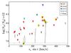 |
Fig. A.1 Nitrogen abundance versus projected rotational velocity for the stars in the VFTS sample with no luminosity class identifier. Colours denote spectral type, where grey indicates no identified spectral type (Walborn et al. 2014). Stars with a yellow circle underlaid are considered poor quality fits. |
Nitrogen abundances of presumed-single O-type giants and supergiants in the VFTS.
Appendix B: Discussion on individual sources
In this paper, we discuss the sample of VFTS O-type giants and supergiants from the viewpoint of a coherent, continuously evolving stellar population (Sect. 5). However, given the spatial and temporal extent of the 30 Dor region covered by the VFTS data (see e.g., Walborn & Blades 1997; Selman et al. 1999; Sabbi et al. 2013, for a discussion), one has to be aware of the diversity within the sample.
We provide here more details on individual stars, that have εN> 7.5 or are otherwise noteworthy, such as the run-away candidates. We discuss their evolutionary state and notable aspects of the spectral fitting, supplemented by findings of Walborn et al. (2014) and Almeida et al. (2017). Walborn et al. presented the spectral classification of this sample, and Almeida et al. present the results of the follow-up radial velocity study on the VFTS O-type stars. This section is organised as follows. We first discuss some general properties of the sample. Next, we discuss the run-away candidates, followed by the confirmed binaries, stars with radial velocity variations that do not resemble a binary orbit, confirmed single stars, and end with stars not included in the sample of Almeida et al. (2017).
General properties: in Fig. B.1 we display the location of stars with measured εN> 7.5 (excluding upper limits, essentially Box 2 stars). Members of this group are found in the field, as well as in the different clusters.
The luminous stars in our sample are on average N-enriched, as can be seen in Fig. 10. Moreover, the stars that show He- as well as N-enrichment (Fig. 13) are on average luminous. Furthermore, it appears that the O2-3 objects are all enhanced in nitrogen to a certain degree.
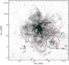 |
Fig. B.1 Spatial distribution of the O-type giants and supergiants with measured εN> 7.5. The locations of the different clusters are indicated. Spectral types O 2-3 are indicated in blue, the O 6-7 in green, and sources of spectral type O 8 and later are coloured red. |
Run-away candidates: VFTS 016, 226 and 306 are classified as run-away candidates. The three stars are moderately rotating with νesini on the order of 100 kms-1 and, interestingly, all occupy the Box 2 region (Fig. 11). The hot star VFTS 016 was also studied by Evans et al. (2010), who estimated a nitrogen abundance of εN ~ 7.9, in good agreement with our result. Its N-abundance can be reproduced by Bonnsai assuming moderate rotation (νesini ~ 170 kms-1) and relatively high inclination (sini ~ 0.8). In the case of VFTS 226 we were not able to extract measurements from the N iii λ4511−4515 lines, although the line profiles resulting from measurements to the (weak) N iii λ4379, 4097 lines are consistent with the data. The N ii λ3995 line is (weakly) predicted by the models, but not present in the data. To reproduce its N-abundance, Bonnsai predicts VFTS 226 is a rapidly rotating star seen almost pole on. VFTS 306 is part of the low gravity sample. The line profiles of N iii λ4195, 4379, 4515, 4535 resulting from our measurement slightly underpredict the observed ones (by  1% of the continuum level), however the models corresponding to the 1σ error on εN typically span the observed data. The N iii λ4097 line is underpredicted by 10% of the continuum and is not used for the abundance measurement.
Confirmed binaries: VFTS 064, 171, 332, 333 and 440 are confirmed by Almeida et al. (2017) as long-period (~103 d) SB1 systems. VFTS 093 was found to be a 250 d binary. VFTS 399 has been extensively discussed by Clark et al. (2015) and is potentially an X-ray binary. Interestingly, for VFTS 333, 399 and 440, our εN measurement agrees within 1σ with the abundance predicted by Bonnsai, based on their evolutionary state. VFTS 064 is N-enriched and shows N iii emission at 4640 Å, which is underpredicted in our best-fit model by ~3% of the continuum. VFTS 093, 171, 332 and 333 are late LC III-II stars with mild N-enrichment (εN in the range 7.3−7.6). In all four cases the profile of N iii λ4097 is underpredicted. As these are long-period systems, their evolution is possibly unaffected by binary interaction (unless they are, e.g., former triples). In the case of VFTS 399, due to blending of the N iii λ4511-4515-4518 complex, we extract an Weq measurement by direct integration. For VFTS 440, Ramírez-Agudelo et al. (2017) report an unsatisfactory fit and parameters must be taken with caution. These 7 sources are kept in the paper as the VFTS sample of presumed single stars is constructed by well-defined criteria (see Sana et al. 2013, for a discussion), benefiting binary population synthesis calculations. However, they are excluded from the comparison in Sect. 5.2.
Nitrogen abundances of presumed-single O-type sources with no luminosity class identifier.
Variable stars: Almeida et al. (2017) find evidence for periodicity in the case of VFTS 259 and 764, however no radial velocity curve could be constructed that would indicate a binary nature. Quasi-periodic oscillations (e.g., pulsations) are possibly the cause of the (small) radial velocity variations. Both sources are classified as LC I, VFTS 259 is the only O-supergiant of intermediate spectral subtype in the VFTS. It has a complicated nitrogen spectrum, as the N iii complex at 4515 Å transitions from absorption into emission at these temperatures (see Fig. 2). In addition, the N iv λ4058 line is predicted in the models but not present in the data. VFTS 764 is tagged as N-strong by Walborn et al. (2014), in agreement with our quantitative results. It is a relatively evolved star (log gc = 2.90). The N ii λ3995 line is not reproduced in parallel to the N iii lines (compared to the data, it is only weakly present in the models). We exclude it from the abundance measurement, as the N iii lines yield consistent results. It remains to be investigated whether the irregular radial velocity variability of VFTS 259 and 764 offers an indication to the nature of their nitrogen enrichment.
Confirmed single stars: in the case of VFTS 087, 267, 178 and 819, Almeida et al. (2017) find no evidence for binarity. VFTS 087 and 178 are evolved supergiants of intermediate mass (~30−35 M⊙). In current evolutionary tracks, such stars are not expected to have lost a significant part of their envelope in prior phases. VFTS 267 is an early-type star with moderate enrichment, that is compatible with the nitrogen content predicted by Bonnsai. For this star we were not able to extract a reliable Weq measurement from its (noisy) N v λ4619 line. The other two lines (N iv λ4058 and N v λ4603) are in excellent agreement, resulting in a very small error bar (σN = 0.03). Taking into account the error on the atmospheric parameters, Ramírez-Agudelo et al. (2017) find a more realistic 1σ uncertainty of ~0.2 dex (see also Sect. 3.4). However, the line profiles of our best-fit model are shifted by ~1 Å and ~2 Å for the N iv and N v profile respectively. VFTS 819 is an ON star of moderate evolutionary mass (22 M⊙) and age (~2 Myr). This source is very enriched in He as well as in N, and, given the high degree of abundance anomaly, is possibly a post-interaction binary. Compared to the tracks of Brott et al. (2011a), it could also be a quasi chemically-homogeneous star rotating initially at ~500 kms-1, seen almost pole-on.
Other enriched sources: the remainder of the stars in our sample was not included in the radial velocity follow-up survey. We comment here on the particularly enriched sources. VFTS 151, 180, 518, 599 and 669 show small but significant radial velocity variations, but were not observed by Almeida et al. (2017) for reasons related to fibre placement constraints. For VFTS 253, 466, 513, 566, 753 and 807, Sana et al. (2013) did not find significant radial velocity variations. We first discuss the early-type stars.
VFTS 180, 518, 566 and 599 are O2-3 stars with high mass-loss rates and high-degrees of N-enrichment. This could, in principle, point to their envelopes being stripped by their strong outflows, revealing chemically enriched layers. This process might be ongoing in VFTS 180 that follows the empirical correlation between surface helium abundance and log (Ṁ/M) reported by Bestenlehner et al. (2011, see also Sect. 6.5.2, but is not
expected for the other sources, since these appear to be rather young objects.
Regarding their individual analyses, the early supergiant VFTS 180 shows very strong He- and N-emission. For this star, we find it challenging to reproduce the N v lines in parallel to lines of other ionisation stages. N v λ4603 presents a P Cygni profile, and a Weq measurement is not appropriate. We excluded N v λ4619 as well because it is not well reproduced using the parameters provided by Ramírez-Agudelo et al. (2017). If we include this line the resulting abundance measurement does not change significantly (yielding εN = 8.70 ± 0.40), due to the relatively large error on its individual abundance measurement (σi = 0.10). The continuum normalisation to the right of the N iii λ4630−4634−4640 complex is shifted by ~3% upwards, to the left it is shifted by ~1.5%. Although the exact degree of N-enrichment is difficult to constrain, it is certainly enriched. For VFTS 518 the best fit model underpredicts the N v lines (at a level of ~2% of the continuum), but fits well the N iii λ4634-4640-4641 and N iv λ4058 lines. This source is also enriched in He. In the cases of VFTS 566 and 599 the best-fit model of the N v lines is slightly shifted (by ~0.5 Å) and underpredicted compared to the data (by ~2% of the continuum).
VFTS 151 is a spatially resolved triple within the VFTS fibre producing a composite spectrum with a large range of types (see Table A.1 of Walborn et al. 2014). We are unable to reproduce the N iv λ4058 line and underpredict the N iii λ4634-4640-4641 complex by 2% of the continuum, while the N iii λ4511-4515-4518 complex, predicted by the best model, appears absent. This star does not make part of the low gravity sample. For VFTS 253 and 513, N-lines are present that have widths consistent with the resolution limit of the survey, even though Ramírez-Agudelo et al. (2017) estimate νesini ~ 100 kms-1 for both sources. Test models with νesini values below the resolution limit provide a satisfactory fit. However, it cannot be excluded that these lines originate from an undetected companion. The fibre of VFTS 513 could be contaminated, but for VFTS 253 this seems not the case. Both stars have rotation-corrected gravities in excess of 4, and VFTS 253 is one of the stars with Si-weak lines (see Walborn et al. 2014). VFTS 466 and 753 are otherwise unremarkable late giants, with N-abundances of ~7.6. VFTS 669 is a late supergiant. It shows emission at N iii λ4640 which is not reproduced by our best fit model. Nevertheless, good agreement is found with the N-abundance determined by Ramírez-Agudelo et al. (2017). VFTS 807 is tagged with N-strong by Walborn et al. (2014), in conformity with our N-measurement. It is a moderately evolved, but not so massive star Mevol = 18.8 M⊙). The origin of the observed N-enrichment in aforementioned stars remains to be investigated.
Finally we note that VFTS 016, 064, 171, 180, 259, 267, 333, 518, 566, 599, 664 and 669 were also studied by Bestenlehner et al. (2011). They provide no nitrogen abundance measurements, but rate stars as nitrogen normal, enhanced, or in-between. These qualitative measures are in general agreement with our quantitative results.
Appendix C: Additional examples of line fits
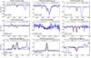 |
Fig. C.1 Examples of line fits for enriched stars, ranging over spectral types and nitrogen ionisation stage used. The observed spectrum is shown in blue, the best fit model in black (the measured εN is annotated in the panel), models representing the upper and lower 1σ error in dashed black, and a FASTWIND model with εN = 7.33 in red. Only one of the lines used is shown for each source. All sources need a significant nitrogen enrichment in order to reproduce the observed profiles. |
All Tables
Number of stars for which the nitrogen abundance could be constrained and for which only upper limits could be derived, as a function of luminosity class.
Nitrogen abundances of presumed-single O-type giants and supergiants in the VFTS.
Nitrogen abundances of presumed-single O-type sources with no luminosity class identifier.
All Figures
|
Fig. 1 Comparison between nitrogen abundances derived with the automated fitting method (vertical axis) and the method described in Sect. 3 (horizontal axis). Dotted lines indicate the nitrogen baseline abundance of LMC stars. The dashed line shows the 1:1 relation. The observed stars are marked with their VFTS ID. Except for two stars the two methods agree within 1σ. Note that ξm is allowed to vary in the automated method, while ξm is fixed at 10 kms-1 for the measurements in this paper (see Sect. 3.4). |
| In the text | |
|
Fig. 2 Equivalent width as a function of effective temperature and nitrogen abundance for several diagnostic lines. Colours, following the rainbow from red to purple, indicate nitrogen abundances εN ranging from 6.93 to 8.53 in steps of 0.4 dex. Negative values of Weq represent emission. For all models: log g = 3.9 (cgs), log Ṁ = −6 (M⊙/ yr) and ξm = 7 kms-1. |
| In the text | |
|
Fig. 3 Abundance measurement for VFTS 466, a relatively high S/N source. Not all lines used are shown. Left panels: the observed spectrum is shown in blue and the best model fit in black. The nitrogen abundance of the best model resulted from combining all utilised lines and is given by the εN in the figure title. The selection of the fit region is displayed in red. Middle panels: zoom in on the fitted region, with the best fit Gaussian profile in red. Right panels: theoretical Weq values as a function of εN (horizontal axis) are shown in black. Measured Weq and interpolated εN are in red and blue, respectively. Dashed red lines indicate the measurement error and dashed blue lines the corresponding uncertainty in the best fit value. |
| In the text | |
|
Fig. 4 Same as Fig. 3, for VFTS 103, typical for relatively low S/N. In the case of the N iii λ4379 line (middle row), no Gaussian profile could be fitted. However, the final line profile that is derived from measurements to other lines, is consistent with the data. |
| In the text | |
|
Fig. 5 Example of a Weq measurement by integration (for VFTS 399). The Weq is extracted by integration of the red region of the spectrum in the left panel. In the middle panel, this is compared to theoretical Weq values of the combined complex as predicted by FASTWIND, yielding εN and its associated error. The robustness of the measurement is checked twofold: first by comparing a model with the final solution to the observed spectrum (left panel, solid black line). Second, in the right panel, by comparing the abundance measurements that result from adjustment of the integration bounds, varying the width Δλ as function of the adopted width Δλ0, where the adopted measurement is indicated by the red triangle. The 1σ error on Weq is calculated through propagation of the error spectrum. |
| In the text | |
|
Fig. 6 VFTS 711, 080, and 109 are examples of cases for which only upper limits could be derived. Left panels: the observed spectrum is shown in blue, the region used to determine the S/N in red, and the model representing the upper limit in black. Middle panels: zoom in on the fitted region. For these cases this region is used to determine the S/N. The red line is the mean flux level of this range; the dashed lines indicate the standard deviation. Right panels: theoretical depth values as a function of εN in black, where the minimal detectable depth and its inferred upper limit are indicated as the red horizontal and the blue vertical line respectively. The resulting upper limit is indicated in the top left corner of the right panel. The line depression for the upper limit to εN can be considerably larger than the noise would suggest as a result of our conservative choice for this limit (see Sect. 3.3). |
| In the text | |
|
Fig. 7 Difference in the measured N-abundance using the micro-turbulent velocity as determined by Ramírez-Agudelo et al. (2017) and ξm = 10 kms-1. All stars for which the nitrogen abundance could be determined are shown. |
| In the text | |
|
Fig. 8 Nitrogen abundance versus projected rotational velocity. For all panels, symbols denote luminosity class and colours spectral type; see legend in the top panel. Top panel: entire sample. The newly detected binaries have a yellow circle underlaid (see Sect. 3.4). Middle panel: subset of stars for which the nitrogen abundance could be measured. Bottom panel: subset of stars for which only upper limits could be derived. The dashed lines indicate detection limits for different S/N and are discussed in Sect. 4. The black solid lines are evolutionary tracks for the O-type stage (Teff ≥ 29 kK) of a 20 M⊙ star (Brott et al. 2011a), with initial rotational velocities of 114, 170, 282 and 390 kms-1. We multiply the rotational velocity of these tracks by π/ 4 to account for the average projection effect. |
| In the text | |
|
Fig. 9 Nitrogen abundance versus projected rotational velocity for the full sample. Symbols indicate luminosity class, colours indicate spectral subtype. Tracks (Brott et al. 2011a) drawn in solid black lines are for a 20 M⊙ star, evolved until the effective temperature is below 29 kK and they become B-type stars. Initial rotational velocities for the tracks are 114, 170, 282 and 390 kms-1 and have been multiplied by π/ 4 to account for the average projection effect. The population synthesis calculation projected in the background is for the O star phase only and assumes a flat distribution of rotational velocities. Out of 740 × 103 simulated stars, 310 × 103 pass the selection criterion (Teff ≥ 29 kK). These are normalised to 72 stars, matching the number of observed stars in the plot. |
| In the text | |
|
Fig. 10 Hertzsprung-Russell Diagram (HRD) for the O-type stars in the VFTS sample, excluding binaries and poor quality fits (Sect. 3.4). Luminosities and temperatures are from Ramírez-Agudelo et al. (2017). Evolutionary sequences and isochrones are from Brott et al. (2011a) and Köhler et al. (2015). The solid tracks alter to dotted tracks for Teff ≤ 29 kK. Grey crosses indicate LC V VFTS stars (Sabín-Sanjulián et al. 2014). The remaining stars are colour-coded according to εN, where upper limits are indicated in blue. Encircled stars have log gc ≤ 3.75, where pink circles indicate that they occupy Box 2 and green circles that they are outside of that box (see Sect. 5.2 and Fig. 11). |
| In the text | |
|
Fig. 11 Nitrogen abundance versus projected rotational velocity for 27 O-type stars with gravities log gc ≤ 3.75. It constitutes all of the VFTS sources fulfilling these criteria, save for three O-dwarfs studied by Sabín-Sanjulián et al. (2014) that would all end up in Box 3 (Símon-Díaz, priv. comm.), binaries and poor quality fits (Sect. 3.4). Identical selection criteria have been applied to the population synthesis calculation projected on the background. The applied initial spin distribution in this calculation is assumed to be that derived for the presumed-single VFTS stars (Ramírez-Agudelo et al. 2013). Out of the 721 × 103 simulated stars, 21 × 103 pass the selection criteria (Teff ≥ 29 kK and log gc ≤ 3.75). These are normalised to 27 stars, matching the number of observed stars in the plot. The boxes, separated by the solid black lines, are defined in Sect. 5.2. |
| In the text | |
|
Fig. 12 Distribution of evolutionary masses for the stars in Fig. 11 that occupy Box 2 (left) and the remainder of stars (right). Black crosses indicate data points. The middle column in each half of the diagram shows the median of the sample in red, where the boxplot indicates the 0.25 and 0.75 percentiles with whiskers extending out no further than 1.5 times the inter-quartile range. The right column indicates the weighted average and standard deviation (in parentheses) of the sample in blue. Evolutionary masses are calculated using the Bonnsai tool (Sect. 6.1). |
| In the text | |
|
Fig. 13 Nitrogen abundance versus surface helium mass fraction. In the background the outcome of population synthesis is projected, as explained in Sect. 5 and shown in Fig. 11. |
| In the text | |
|
Fig. A.1 Nitrogen abundance versus projected rotational velocity for the stars in the VFTS sample with no luminosity class identifier. Colours denote spectral type, where grey indicates no identified spectral type (Walborn et al. 2014). Stars with a yellow circle underlaid are considered poor quality fits. |
| In the text | |
|
Fig. B.1 Spatial distribution of the O-type giants and supergiants with measured εN> 7.5. The locations of the different clusters are indicated. Spectral types O 2-3 are indicated in blue, the O 6-7 in green, and sources of spectral type O 8 and later are coloured red. |
| In the text | |
|
Fig. C.1 Examples of line fits for enriched stars, ranging over spectral types and nitrogen ionisation stage used. The observed spectrum is shown in blue, the best fit model in black (the measured εN is annotated in the panel), models representing the upper and lower 1σ error in dashed black, and a FASTWIND model with εN = 7.33 in red. Only one of the lines used is shown for each source. All sources need a significant nitrogen enrichment in order to reproduce the observed profiles. |
| In the text | |
Current usage metrics show cumulative count of Article Views (full-text article views including HTML views, PDF and ePub downloads, according to the available data) and Abstracts Views on Vision4Press platform.
Data correspond to usage on the plateform after 2015. The current usage metrics is available 48-96 hours after online publication and is updated daily on week days.
Initial download of the metrics may take a while.