| Issue |
A&A
Volume 586, February 2016
|
|
|---|---|---|
| Article Number | A138 | |
| Number of page(s) | 29 | |
| Section | Interstellar and circumstellar matter | |
| DOI | https://doi.org/10.1051/0004-6361/201525896 | |
| Published online | 09 February 2016 | |
Planck intermediate results
XXXV. Probing the role of the magnetic field in the formation of structure in molecular clouds
1 APC, AstroParticule et Cosmologie, Université Paris Diderot, CNRS/IN2P3, CEA/lrfu, Observatoire de Paris, Sorbonne Paris Cité, 10 rue Alice Domon et Léonie Duquet, 75205 Paris Cedex 13, France
2 African Institute for Mathematical Sciences, 6–8 Melrose Road, Muizenberg, Cape Town, South Africa
3 Agenzia Spaziale Italiana Science Data Center, via del Politecnico snc, 00133 Roma, Italy
4 Aix-Marseille Université, CNRS, LAM (Laboratoire d’Astrophysique de Marseille) UMR 7326, 13388 Marseille, France
5 Astrophysics Group, Cavendish Laboratory, University of Cambridge, J J Thomson Avenue, Cambridge CB3 0HE, UK
6 Astrophysics & Cosmology Research Unit, School of Mathematics, Statistics & Computer Science, University of KwaZulu-Natal, Westville Campus, Private Bag X54001, Durban 4000, South Africa
7 CITA, University of Toronto, 60 St. George St., Toronto, ON M5S 3H8, Canada
8 CNRS, IRAP, 9 Av. colonel Roche, BP 44346, 31028 Toulouse Cedex 4, France
9 California Institute of Technology, Pasadena, California, USA
10 Centro de Estudios de Física del Cosmos de Aragón (CEFCA), Plaza San Juan, 1, planta 2, 44001 Teruel, Spain
11 Computational Cosmology Center, Lawrence Berkeley National Laboratory, Berkeley, California, USA
12 DSM/Irfu/SPP, CEA-Saclay, 91191 Gif-sur-Yvette Cedex, France
13 DTU Space, National Space Institute, Technical University of Denmark, Elektrovej 327, 2800 Kgs. Lyngby, Denmark
14 Département de Physique Théorique, Université de Genève, 24 quai E. Ansermet, 1211 Genève 4, Switzerland
15 Departamento de Astrofísica, Universidad de La Laguna (ULL), 38206 La Laguna, Tenerife, Spain
16 Departamento de Física, Universidad de Oviedo, Avda. Calvo Sotelo s/n, 33007 Oviedo, Spain
17 Department of Astronomy and Astrophysics, University of Toronto, 50 Saint George Street, Toronto, ON M5 S Ontario, Canada
18 Department of Astrophysics/IMAPP, Radboud University Nijmegen, PO Box 9010, 6500 GL Nijmegen, The Netherlands
19 Department of Physics & Astronomy, University of British Columbia, 6224 Agricultural Road, Vancouver, BC V6T 1Z1 British Columbia, Canada
20 Department of Physics and Astronomy, Dana and David Dornsife College of Letter, Arts and Sciences, University of Southern California, Los Angeles, CA 90089, USA
21 Department of Physics and Astronomy, University College London, London WC1E 6BT, UK
22 Department of Physics, Florida State University, Keen Physics Building, 77 Chieftan Way, Tallahassee, FL 32306, USA
23 Department of Physics, Gustaf Hällströmin katu 2a, University of Helsinki, 00014 Helsinki, Finland
24 Department of Physics, Princeton University, Princeton, NJ 08544-0708, USA
25 Department of Physics, University of California, Santa Barbara, CA 93106, USA
26 Department of Physics, University of Illinois at Urbana-Champaign, 1110 West Green Street, Urbana, IL 61801, USA
27 Dipartimento di Fisica e Astronomia G. Galilei, Università degli Studi di Padova, via Marzolo 8, 35131 Padova, Italy
28 Dipartimento di Fisica e Scienze della Terra, Università di Ferrara, via Saragat 1, 44122 Ferrara, Italy
29 Dipartimento di Fisica, Università La Sapienza, P.le A. Moro 2, 00185 Roma, Italy
30 Dipartimento di Fisica, Università degli Studi di Milano, via Celoria, 16, 20133 Milano, Italy
31 Dipartimento di Fisica, Università degli Studi di Trieste, via A. Valerio 2, 34128 Trieste, Italy
32 Dipartimento di Matematica, Università di Roma Tor Vergata, via della Ricerca Scientifica, 1, 00133 Roma, Italy
33 Discovery Center, Niels Bohr Institute, Blegdamsvej 17, 2100 Copenhagen, Denmark
34 Escola de Artes, Ciências e Humanidades, Universidade de São Paulo, Rua Arlindo Bettio 1000, CEP 03828-000, São Paulo, Brazil
35 European Space Agency, ESAC, Planck Science Office, Camino bajo del Castillo, s/n, Urbanización Villafranca del Castillo, Villanueva de la Cañada, 28691 Madrid, Spain
36 European Space Agency, ESTEC, Keplerlaan 1, 2201 AZ Noordwijk, The Netherlands
37 Facoltà di Ingegneria, Università degli Studi e-Campus, via Isimbardi 10, Novedrate (CO), 22060, Italy
38 Gran Sasso Science Institute, INFN, viale F. Crispi 7, 67100 L’ Aquila, Italy
39 HGSFP and University of Heidelberg, Theoretical Physics Department, Philosophenweg 16, 69120 Heidelberg, Germany
40 Helsinki Institute of Physics, Gustaf Hällströmin katu 2, University of Helsinki, 00100 Helsinki, Finland
41 INAF–Osservatorio Astrofisico di Catania, via S. Sofia 78, 95123 Catania, Italy
42 INAF–Osservatorio Astronomico di Padova, Vicolo dell’Osservatorio 5, 35122 Padova, Italy
43 INAF–Osservatorio Astronomico di Roma, via di Frascati 33, 00078 Monte Porzio Catone, Italy
44 INAF–Osservatorio Astronomico di Trieste, via G.B. Tiepolo 11, Trieste, Italy
45 INAF/IASF Bologna, via Gobetti 101, 40129 Bologna, Italy
46 INAF/IASF Milano, via E. Bassini 15, 20133 Milano, Italy
47 INFN, Sezione di Bologna, via Irnerio 46, 40126 Bologna, Italy
48 INFN, Sezione di Roma 1, Università di Roma Sapienza, P.le Aldo Moro 2, 00185 Roma, Italy
49 INFN, Sezione di Roma 2, Università di Roma Tor Vergata, via della Ricerca Scientifica, 1 Roma, Italy
50 INFN/National Institute for Nuclear Physics, via Valerio 2, 34127 Trieste, Italy
51 IPAG: Institut de Planétologie et d’Astrophysique de Grenoble, Université Grenoble Alpes, IPAG, 38000 Grenoble, France, CNRS, IPAG, 38000 Grenoble, France
52 Imperial College London, Astrophysics group, Blackett Laboratory, Prince Consort Road, London, SW7 2AZ, UK
53 Infrared Processing and Analysis Center, California Institute of Technology, Pasadena, CA 91125, USA
54 Institut Néel, CNRS, Université Joseph Fourier Grenoble I, 25 rue des Martyrs, 38042 Grenoble, France
55 Institut Universitaire de France, 103 bd Saint-Michel, 75005 Paris, France
56 Institut d’Astrophysique Spatiale, CNRS (UMR 8617) Université Paris-Sud 11, Bâtiment 121, 91400 Orsay, France
57 Institutd’Astrophysique de Paris, CNRS (UMR 7095), 98bis boulevard Arago, 75014 Paris, France
58 Institute of Astronomy, University of Cambridge, Madingley Road, Cambridge CB3 0HA, UK
59 Institute of Theoretical Astrophysics, University of Oslo, Blindern, 0315 Oslo, Norway
60 Instituto de Astrofísica de Canarias, C/vía Láctea s/n, La Laguna 38205 Tenerife, Spain
61 Instituto de Física de Cantabria (CSIC-Universidad de Cantabria), Avda. de los Castros s/n, 39005 Santander, Spain
62 Istituto Nazionale di Fisica Nucleare, Sezione di Padova, via Marzolo 8, 35131 Padova, Italy
63 Jet Propulsion Laboratory, California Institute of Technology, 4800 Oak Grove Drive, Pasadena, California, USA
64 Jodrell Bank Centre for Astrophysics, Alan Turing Building, School of Physics and Astronomy, The University of Manchester, Oxford Road, Manchester, M13 9PL, UK
65 Kavli Institute for Cosmological Physics, University of Chicago, Chicago, IL 60637, USA
66 Kavli Institute for Cosmology Cambridge, Madingley Road, Cambridge, CB3 0HA, UK
67 Kazan Federal University, 18 Kremlyovskaya St., 420008 Kazan, Russia
68 LAL, Université Paris-Sud, CNRS/IN2P3, 91405 Orsay, France
69 LERMA, CNRS, Observatoire de Paris, 61 avenue de l’Observatoire, 75014 Paris, France
70 Laboratoire AIM, IRFU/Service d’Astrophysique – CEA/DSM – CNRS – Université Paris Diderot, Bât. 709, CEA-Saclay, 91191 Gif-sur-Yvette Cedex, France
71 Laboratoire Traitement et Communication de l’Information, CNRS (UMR 5141) and Télécom ParisTech, 46 rue Barrault 75634 Paris Cedex 13, France
72 Laboratoire de Physique Subatomique et Cosmologie, Université Grenoble-Alpes, CNRS/IN2P3, 53 rue des Martyrs, 38026 Grenoble Cedex, France
73 Laboratoire de Physique Théorique, Université Paris-Sud 11 & CNRS, Bâtiment 210, 91405 Orsay, France
74 Lawrence Berkeley National Laboratory, Berkeley, California, USA
75 Lebedev Physical Institute of the Russian Academy of Sciences, Astro Space Centre, 84/32 Profsoyuznaya st., Moscow, GSP-7, 117997, Russia
76 Max-Planck-Institut für Astrophysik, Karl-Schwarzschild-Str. 1, 85741 Garching, Germany
77 National University of Ireland, Department of Experimental Physics, Maynooth, Co. Kildare, Ireland
78 Nicolaus Copernicus Astronomical Center, Bartycka 18, 00-716 Warsaw, Poland
79 Niels Bohr Institute, Blegdamsvej 17, 2100 Copenhagen, Denmark
80 Optical Science Laboratory, University College London, Gower Street, London WC1E 6BT, UK
81 SISSA, Astrophysics Sector, via Bonomea 265, 34136, Trieste, Italy
82 SUPA, Institute for Astronomy, University of Edinburgh, Royal Observatory, Blackford Hill, Edinburgh EH9 3HJ, UK
83 School of Physics and Astronomy, Cardiff University, Queens Buildings, The Parade, Cardiff, CF24 3AA, UK
84 Sorbonne Université-UPMC, UMR 7095, Institut d’Astrophysique de Paris, 98bis boulevard Arago, 75014 Paris, France
85 Space Sciences Laboratory, University of California, Berkeley, CA 94720, USA
86 Special Astrophysical Observatory, Russian Academy of Sciences, Nizhnij Arkhyz, Zelenchukskiy region, 369167 Karachai-Cherkessian Republic, Russia
87 Sub-Department of Astrophysics, University of Oxford, Keble Road, Oxford OX1 3RH, UK
88 UPMC Univ Paris 06, UMR 7095, 98bis boulevard Arago, 75014 Paris, France
89 Université de Toulouse, UPS-OMP, IRAP, 31028 Toulouse Cedex 4, France
90 University of Granada, Departamento de Física Teórica y del Cosmos, Facultad de Ciencias, 18071 Granada, Spain
91 University of Granada, Instituto Carlos I de Física Teórica y Computacional, 18071 Granada, Spain
92 Warsaw University Observatory, Aleje Ujazdowskie 4, 00-478 Warszawa, Poland
Received: 13 February 2015
Accepted: 25 May 2015
Abstract
Within ten nearby (d < 450 pc) Gould belt molecular clouds we evaluate statistically the relative orientation between the magnetic field projected on the plane of sky, inferred from the polarized thermal emission of Galactic dust observed by Planck at 353 GHz, and the gas column density structures, quantified by the gradient of the column density, NH. The selected regions, covering several degrees in size, are analysed at an effective angular resolution of 10′ FWHM, thus sampling physical scales from 0.4 to 40 pc in the nearest cloud. The column densities in the selected regions range from NH≈ 1021 to1023 cm-2, and hence they correspond to the bulk of the molecular clouds. The relative orientation is evaluated pixel by pixel and analysed in bins of column density using the novel statistical tool called “histogram of relative orientations”. Throughout this study, we assume that the polarized emission observed by Planck at 353 GHz is representative of the projected morphology of the magnetic field in each region, i.e., we assume a constant dust grain alignment efficiency, independent of the local environment. Within most clouds we find that the relative orientation changes progressively with increasing NH, from mostly parallel or having no preferred orientation to mostly perpendicular. In simulations of magnetohydrodynamic turbulence in molecular clouds this trend in relative orientation is a signature of Alfvénic or sub-Alfvénic turbulence, implying that the magnetic field is significant for the gas dynamics at the scales probed by Planck. We compare the deduced magnetic field strength with estimates we obtain from other methods and discuss the implications of the Planck observations for the general picture of molecular cloud formation and evolution.
Key words: ISM: general / ISM: magnetic fields / ISM: clouds / dust, extinction / submillimeter: ISM / infrared: ISM
Corresponding author: Juan D. Soler, This email address is being protected from spambots. You need JavaScript enabled to view it.
© ESO, 2016
1. Introduction
The formation and evolution of molecular clouds (MCs) and their substructures, from filaments to cores and eventually to stars, is the product of the interaction between turbulence, magnetic fields, and gravity (Bergin & Tafalla 2007; McKee & Ostriker 2007). The study of the relative importance of these dynamical processes is limited by the observational techniques used to evaluate them. These limitations have been particularly critical when integrating magnetic fields into the general picture of MC dynamics (Elmegreen & Scalo 2004; Crutcher 2012; Heiles & Haverkorn 2012; Hennebelle & Falgarone 2012).
There are two primary methods of measuring magnetic fields in the dense interstellar medium (ISM). First, observation of the Zeeman effect in molecular lines provides the line-of-sight component of the field B∥ (Crutcher 2005). Second, polarization maps – in extinction from background stars and emission from dust – reveal the orientation of the field averaged along the line of sight and projected on the plane of the sky (Hiltner 1949; Davis & Greenstein 1951; Hildebrand 1988; Planck Collaboration Int. XXI 2015).
Analysis of the Zeeman effect observations presented by Crutcher et al. (2010) shows that in the diffuse ISM sampled by Hi lines (nH< 300 cm-3), the maximum magnetic field strength Bmax does not scale with density. This is interpreted as the effect of diffuse clouds assembled by flows along magnetic field lines, which would increase the density but not the magnetic field strength. In the denser regions (nH> 300 cm-3), probed by OH and CN spectral lines, the same study reports a scaling of the maximum magnetic field strength  . The latter observation can be interpreted as the effect of isotropic contraction of gas too weakly magnetized for the magnetic field to affect the morphology of the collapse. However, given that the observations are restricted to pencil-like lines of sight and the molecular tracers are not homogeneously distributed, the Zeeman effect measurements alone are not sufficient to determine the relative importance of the magnetic field at the multiple scales within MCs.
The observation of starlight polarization provides an estimate of the projected magnetic field orientation in particular lines of sight. Starlight polarization observations show coherent magnetic fields around density structures in MCs (Pereyra & Magalhães 2004; Franco et al. 2010; Sugitani et al. 2011; Chapman et al. 2011; Santos et al. 2014). The coherent polarization morphology can be interpreted as the result of dynamically important magnetic fields. However, these observations alone are not sufficient to map even the projected magnetic field morphology fully and in particular do not tightly constrain the role of magnetic fields in the formation of structure inside MCs.
The study of magnetic field orientation within the MCs is possible through the observation of polarized thermal emission from dust. Far-infrared and submillimetre polarimetric observations have been limited to small regions up to hundreds of square arcminutes within clouds (Li et al. 2006; Matthews et al. 2014) or to large sections of the Galactic plane at a resolution of several degrees (Benoît et al. 2004; Bierman et al. 2011). On the scale of prestellar cores and cloud segments, these observations reveal both significant levels of polarized emission and coherent field morphologies (Ward-Thompson et al. 2000; Dotson et al. 2000; Matthews et al. 2009).
The strength of the magnetic field projected on the plane of the sky (B⊥) can be estimated from polarization maps using the Davis-Chandrasekhar-Fermi (DCF) method (Davis 1951; Chandrasekhar & Fermi 1953). As discussed in Appendix D, it is assumed that the dispersion in polarization angle ςψ1 is entirely due to incompressible and isotropic turbulence. Turbulence also affects the motion of the gas and so broadens profiles of emission and absorption lines, as quantified by dispersion σv∥. In the DCF interpretation B⊥ is proportional to the ratio σv∥/ςψ. Application of the DCF method to subregions of the Taurus MC gives estimates of B⊥ ≈ 10 μG in low-density regions and ≈ 25 to ≈ 42 μG inside filamentary structures (Chapman et al. 2011). Values of B⊥ ≈ 760 μG have been found in dense parts of the Orion MC region (Houde et al. 2009). Because of the experimental difficulties involved in producing large polarization maps, a complete statistical study of the magnetic field variation across multiple scales is not yet available.
Additional information on the effects of the magnetic field on the cloud structure is found by studying the magnetic field orientation inferred from polarization observations relative to the orientation of the column density structures. Patterns of relative orientation have been described qualitatively in simulations of magnetohydrodynamic (MHD) turbulence with different degrees of magnetization. This is quantified as half the ratio of the gas pressure to the mean-field magnetic pressure (Ostriker et al. 2001; Heitsch et al. 2001), with the resulting turbulence ranging from sub-Alfvénic to super-Alfvénic. Quantitative analysis of simulation cubes, where the orientation of B is available directly, reveals a preferred orientation relative to density structures that depends on the initial magnetization of the cloud (Hennebelle 2013; Soler et al. 2013). Using simple models of dust grain alignment and polarization efficiency to produce synthetic observations of the simulations, Soler et al. (2013) showed that the preferred relative orientation and its systematic dependence on the degree of magnetization are preserved.
Observational studies of relative orientation have mostly relied on visual inspection of polarization maps (e.g., Myers & Goodman 1991; Dotson 1996). This is adequate for evaluating general trends in the orientation of the field. However, it is limited ultimately by the need to represent the field orientation with pseudo-vectors, because when a large polarization map is to be overlaid on a scalar-field map, such as intensity or column density, only a selection of pseudo-vectors can be plotted. On the one hand, if the plotted pseudo-vectors are the result of averaging the Stokes parameters over a region, then the combined visualization illustrates different scales in the polarization and in the scalar field. On the other hand, if the plotted pseudo-vectors correspond to the polarization in a particular pixel, then the illustrated pattern is influenced by small-scale fluctuations that might not be significant in evaluating any trend in relative orientation.
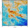 |
Fig. 1 Magnetic field and column density measured by Planck towards the Taurus MC. The colours represent column density. The “drapery” pattern, produced using the line integral convolution method (LIC, Cabral & Leedom 1993), indicates the orientation of magnetic field lines, orthogonal to the orientation of the submillimetre polarization. |
Tassis et al. (2009) present a statistical study of relative orientation between structures in the intensity and the inferred magnetic field from polarization measured at 350μm towards 32 Galactic clouds in maps of a few arcminutes in size. Comparing the mean direction of the field to the semi-major axis of each cloud, they find that the field is mostly perpendicular to that axis. Similarly, Li et al. (2013) compared the relative orientation in 13 clouds in the Gould Belt, calculating the main cloud orientation from the extinction map and the mean orientation of the intercloud magnetic field from starlight polarization. That study reported a bimodal distribution of relative cloud and field orientations; that is, some MCs are oriented perpendicular and some parallel to the mean orientation of the intercloud field. In both studies each cloud constitutes one independent observation of relative orientation, so that the statistical significance of each study depends on the total number of clouds observed. In a few regions of smaller scales, roughly a few tenths of a parsec, Koch et al. (2013) report a preferred orientation of the magnetic field, inferred from polarized dust emission, parallel to the gradient of the emission intensity.
By measuring the intensity and polarization of thermal emission from Galactic dust over the whole sky and down to scales that probe the interiors of nearby MCs, Planck2 provides an unprecedented data set from a single instrument and with a common calibration scheme, for studying the morphology of the magnetic field in MCs and the surrounding ISM, as illustrated for the Taurus region in Fig. 1. We present a quantitative analysis of the relative orientation in a set of nearby (d< 450 pc) well-known MCs to quantify the role of the magnetic field in the formation of density structures on physical scales ranging from tens of parsecs to approximately one parsec in the nearest clouds.
The present work is an extension of previous findings, as reported by the Planck collaboration, on their study of the polarized thermal emission from Galactic dust. Previous studies include an overview of this emission (Planck Collaboration Int. XIX 2015), which reported dust polarization percentages up to 20% at low NH, decreasing systematically with increasing NH to a low plateau for regions with NH> 1022 cm-2. Planck Collaboration Int. XX (2015) presented a comparison of the polarized thermal emission from Galactic dust with results from simulations of MHD turbulence, focusing on the statistics of the polarization fractions and angles. Synthetic observations were made of the simulations under the simple assumption of homogeneous dust grain alignment efficiency. Both studies reported that the largest polarization fractions are reached in the most diffuse regions. Additionally, there is an anti-correlation between the polarization percentage and the dispersion of the polarization angle. This anti-correlation is reproduced well by the synthetic observations, indicating that it is essentially caused by the turbulent structure of the magnetic field.
Over most of the sky Planck Collaboration Int. XXXII (2016) analysed the relative orientation between density structures, which is characterized by the Hessian matrix, and polarization, revealing that most of the elongated structures (filaments or ridges) have counterparts in the Stokes Q and U maps. This implies that in these structures, the magnetic field has a well-defined mean direction on the scales probed by Planck. Furthermore, the ridges are predominantly aligned with the magnetic field measured on the structures. This statistical trend becomes more striking for decreasing column density and, as expected from the potential effects of projection, for increasing polarization fraction. There is no alignment for the highest column density ridges in the NH ≳ 1022 cm-2 sample. Planck Collaboration Int. XXXIII (2016) studied the polarization properties of three nearby filaments, showing by geometrical modelling that the magnetic field in those representative regions has a well-defined mean direction that is different from the field orientation in the surroundings.
In the present work, we quantitatively evaluate the relative orientation of the magnetic field inferred from the Planck polarization observations with respect to the gas column density structures, using the histogram of relative orientations (HRO, Soler et al. 2013). The HRO is a novel statistical tool that quantifies the relative orientation of each polarization measurement with respect to the column density gradient, making use of the unprecedented statistics provided by the Planck polarization observations. The HRO can also be evaluated in both 3D simulation data cubes and synthetic observations, thereby providing a direct comparison between observations and the physical conditions included in MHD simulations. We compare the results of the HRO applied to the Planck observations with the results of the same analysis applied to synthetic observations of MHD simulations of super-Alfvénic, Alfvénic, and sub-Alfvénic turbulence.
Thus by comparison with numerical simulations of MHD turbulence, the HRO provides estimates of the magnetic field strength without any of the assumptions involved in the DCF method. For comparison, we estimate B⊥ using the DCF method and the related method described by Hildebrand et al. (2009; DCF+SF, for DCF plus structure function) and provide a critical assessment of their applicability.
This paper is organized as follows. Section 2 introduces the Planck353 GHz polarization observations, the gas column density maps, and the CO line observations used to derive the velocity information. The particular regions where we evaluate the relative orientation between the magnetic field and the column density structures are presented in Sect. 3. Section 4 describes the statistical tools used for the study of these relative orientations. In Sect. 5 we discuss our results and their implications in the general picture of cloud formation. Finally, Sect. 6 summarizes the main results. Additional information on the selection of the polarization data, the estimation of uncertainties affecting the statistical method, and the statistical significance of the relative orientation studies can be found in Appendices A−C, respectively. Appendix D presents alternative estimates of the magnetic field strength in each region.
2. Data
2.1. Thermal dust polarization
Over the whole sky Planck observed the linear polarization (Stokes Q and U) in seven frequency bands from 30 to 353 GHz (Planck Collaboration I 2014). In this study, we used data from the High Frequency Instrument (HFI, Lamarre et al. 2010) at 353 GHz, the highest frequency band that is sensitive to polarization. Towards MCs the contribution of the cosmic microwave background (CMB) polarized emission is negligible at 353 GHz, making this the Planck map that is best suited to studying the spatial structure of the dust polarization (Planck Collaboration Int. XIX 2015; Planck Collaboration Int. XX 2015).
We used the Stokes Q and U maps and the associated noise maps made from five independent consecutive sky surveys of the Planck cryogenic mission, which together correspond to the DR3 (delta-DX11d) internal data release. We refer to previous Planck publications for the data processing, map making, photometric calibration, and photometric uncertainties (Planck Collaboration II 2014; Planck Collaboration V 2014; Planck Collaboration VI 2014; Planck Collaboration VIII 2014). As in the first Planck polarization papers, we used the International Astronomical Union (IAU) conventions for the polarization angle, measured from the local direction to the north Galactic pole with positive values increasing towards the east.
The maps of Q, U, their respective variances  ,
,  , and their covariance σQU are initially at
  resolution in HEALPix format3 with a pixelization at Nside = 2048, which corresponds to an effective pixel size of
  . To increase the signal-to-noise ratio (S/N) of extended emission, we smoothed all the maps to 10′ resolution using a Gaussian approximation to the Planck beam and the covariance smoothing procedures described in Planck Collaboration Int. XIX (2015).
The maps of the individual regions are projected and resampled onto a Cartesian grid by using the gnomonic projection procedure described in Paradis et al. (2012). The HRO analysis is performed on these projected maps.
2.2. Column density
We used the dust optical depth at 353 GHz (τ353) as a proxy for the gas column density (NH). The τ353 map (Planck Collaboration XI 2014) was derived from the all-sky Planck intensity observations at 353, 545, and 857 GHz, and the IRAS observations at 100μm, which were fitted using a modified black body spectrum. Other parameters obtained from this fit are the temperature and the spectral index of the dust opacity. The τ353 map, computed initially at 5′ resolution, was smoothed to 10′ to match the polarization maps. The errors resulting from smoothing the product τ353 map, rather than the underlying data, are negligible compared to the uncertainties in the dust opacity and do not significantly affect the results of this study.
To scale from τ353 to NH, following Planck Collaboration XI (2014), we adopted the dust opacity found using Galactic extinction measurements of quasars,  (1)
(1)
Variations in dust opacity are present even in the diffuse ISM and the opacity increases systematically by a factor of 2 from the diffuse to the denser ISM (Planck Collaboration XXIV 2011; Martin et al. 2012; Planck Collaboration XI 2014), but our results do not critically depend on this calibration.
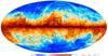 |
Fig. 2 Locations and sizes of the regions selected for analysis. The background map is the gas column density, NH, derived from the dust optical depth at 353 GHz (Planck Collaboration XI 2014). |
Locations and properties of the selected regions.
3. Analysed regions
The selected regions, shown in Fig. 2, correspond to nearby (d< 450 pc) MCs, whose characteristics are well studied and can be used for cloud-to-cloud comparison (Poppel 1997; Reipurth 2008). Their properties are summarized in Table 1, which includes: Galactic longitude l and latitude b at the centre of the field; field size Δl × Δb; estimate of distance; mean and maximum total column densities from dust, ⟨NH⟩ and  , respectively; and mean H2 column density from CO.
In the table the regions are organized from the nearest to the farthest in three groups: (a) regions located at d ≈ 150 pc, namely Taurus, Ophiuchus, Lupus, Chamaeleon-Musca, and Corona Australis (CrA); (b) regions located at d ≈ 300 pc, Aquila Rift and Perseus; and (c) regions located at d ≈ 450 pc, IC 5146, Cepheus, and Orion.
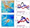 |
Fig. 3 Left: columm density map, log 10(NH/ cm-2), overlaid with magnetic field pseudo-vectors whose orientations are inferred from the Planck 353 GHz polarization observations. The length of the pseudo-vectors is normalized so does not reflect the polarization fraction. In this first group, the regions analysed are, from top to bottom, Taurus, Ophiuchus, Lupus, Chamaeleon-Musca, and CrA. Right: HROs for the lowest, an intermediate, and the highest NH bin (black, blue, and red, respectively). For a given region, bins have equal numbers of selected pixels (see Sect. 4.1.1 and Appendix A) within the NH ranges labelled. The intermediate bin corresponds to selected pixels near the blue contours in the column density images. The horizontal dashed line corresponds to the average per angle bin of 15°. The widths of the shaded areas for each histogram correspond to the ± 1σ uncertainties related to the histogram binning operation. Histograms peaking at 0° correspond to B⊥ predominantly aligned with iso-NH contours. Histograms peaking at 90° and/or − 90° correspond to B⊥ predominantly perpendicular to iso-NH contours. |
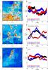 |
Fig. 3 continued. |
Among the clouds in the first group (all shown in Fig. 3, left column) are Ophiuchus and Lupus, which are two regions with different star-forming activities but are close neighbours within an environment disturbed by the Sco-Cen OB association (Wilking et al. 2008; Comerón 2008). Chamaeleon-Musca is a region evolving in isolation,and it is relatively unperturbed (Luhman 2008). Taurus (see also Fig. 1), a cloud with low-mass star formation, appears to be formed by the material swept up by an ancient superbubble centred on the Cas-Tau group (Kenyon et al. 2008). Finally, CrA is one of the nearest regions with recent intermediate- and low-mass star formation, possibly formed by a high-velocity cloud impact on the Galactic plane (Neuhäuser & Forbrich 2008).
In the second group we consider Aquila Rift and Perseus, shown in Fig. 4 (left column). Aquila Rift is a large complex of dark clouds where star formation proceeds in isolated pockets (Eiroa et al. 2008; Prato et al. 2008). The Perseus MC is the most active site of on-going star formation within 300 pc of the Sun. It features a large velocity gradient and is located close to hot stars that might have impacted its structure (Bally et al. 2008).
In the third group are IC 5146, Cepheus, and Orion, shown in Fig. 5 (left column). IC 5146 is an MC complex in Cygnus. It includes an open cluster surrounded by a bright optical nebulosity called the Cocoon nebula, and a region of embedded lower-mass star formation known as the IC 5146 Northern4 Streamer (Harvey et al. 2008). The Cepheus Flare, called simply Cepheus in this study, is a large complex of dark clouds that seems to belong to an even larger expanding shell from an old supernova remnant (Kun et al. 2008). Orion is a dark cloud complex with on-going high and low mass star formation, whose structure appears to be affected by multiple nearby hot stars (Bally 2008).
When taking background/foreground emission and noise within these regions into account, pixels are selected for analysis according to criteria for the gradient of the column density (Appendix A.2) and the polarization (Appendix A.2).
4. Statistical study of the relative orientation of the magnetic field and column density structure
4.1. Methodology
4.1.1. Histogram of relative orientations
We quantify the relative orientation of the magnetic field with respect to the column density structures using the HRO (Soler et al. 2013). The column density structures are characterized by their gradients, which are by definition perpendicular to the iso-column density curves (see calculation in Appendix B.1). The gradient constitutes a vector field that we compare pixel by pixel to the magnetic field orientation inferred from the polarization maps.
In practice we use τ353 as a proxy for NH (Sect. 2.2). The angle φ between B⊥ and the tangent to the τ353 contours is evaluated using5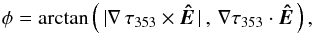 (2)where, as illustrated in Fig. 6, ∇ τ353 is perpendicular to the tangent of the iso-τ353 curves, the orientation of the unit polarization pseudo-vector Ê, perpendicular to B⊥, is characterized by the polarization angle
 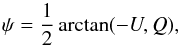 (3)and in Eq. (2), as implemented, the norm actually carries a sign when the range used for φ is between − 90° and 90°.
The uncertainties in φ due to the variance of the τ353 map and the noise properties of Stokes Q and U at each pixel are characterized in Appendix B.
The gradient technique is one of multiple methods for characterizing the orientation of structures in a scalar field. Other methods, which include the Hessian matrix analysis (Molinari et al. 2011; Planck Collaboration Int. XXXII 2016) and the inertia matrix (Hennebelle 2013), are appropriate for measuring the orientation of ridges, i.e., the central regions of filamentary structures. The gradient technique is sensitive to contours and in that sense it is better suited to characterizing changes in the relative orientation in extended regions, not just on the crests of structures (Soler et al. 2013; Planck Collaboration Int. XXXII 2016). Additionally, the gradient technique can sample multiple scales by increasing the size of the vicinity of pixels used for its calculation (derivative kernel; see Appendix B.1). Previous studies that assign an average orientation of the cloud (Tassis et al. 2009; Li et al. 2013) are equivalent to studying the relative orientation using a derivative kernel close to the cloud size.
The selected pixels belong to the regions of each map where the magnitude of the gradient | ∇τ353 | is greater than in a diffuse reference field (Appendix A). This selection criterion aims at separating the structure of the cloud from the structure of the background using the reference field as a proxy. For each region the selected reference field is the region with the same size and Galactic latitude that has the lowest average NH (see Appendix A.1).
In addition to the selection on | ∇τ353 |, we only consider pixels where the norms of the Stokes Q and U are larger than in the diffuse reference field, therefore minimizing the effect of background/foreground polarization external to the cloud. The relative orientation angle, φ, is computed by using polarization measurements with a high S/N in Stokes Q and U, i.e., only considering pixels with | Q | /σQ or | U | /σU> 3. This selection allows the unambiguous definition of Ê by constraining the uncertainty in the polarization angle (see Appendix A.2).
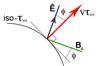 |
Fig. 6 Schematic of the vectors involved in the calculation of the relative orientation angle φ. |
Once we have produced a map of relative orientations for selected pixels following Eq. (2), we divide the map into bins of NH containing an equal number of pixels and generate a histogram of φ for each bin. The shape of the histogram is used to evaluate the preferred relative orientation in each bin directly. A concave histogram, peaking at 0°, corresponds to the preferred alignment of B⊥ with the NH contours. A convex histogram, peaking at 90° and/or − 90°, corresponds to the preferred orientation of B⊥ perpendicular to the NH contours.
The HROs in each region are computed in 25 NH bins having equal numbers of selected pixels (10 bins in two regions with fewer pixels, CrA and IC 5146). The number of NH bins is determined by requiring enough bins to resolve the highest NH regions and at the same time maintaining enough pixels per NH bin to obtain significant statistics from each histogram. The typical number of pixels per bin of NH ranges from approximately 600 in CrA to around 4000 in Chamaeleon-Musca. We use 12 angle bins of width 15°.
The HROs of the first group of regions, the nearest at d ≈ 150 pc, are shown in the right-hand column of Fig. 3. For the sake of clarity, we only present the histograms that correspond to three bins, namely the lowest and highest NH and an intermediate NHvalue. The intermediate bin is the 12th (sixth in two regions with fewer pixels, CrA and IC 5146), and it corresponds to pixels near the blue contour in the image in the left-hand column of Fig. 3. The widths of the shaded areas for each histogram correspond to the 1σ uncertainties related to the histogram binning operation, which are greater than the uncertainties produced by the variances of Q, U, and τ353 (Appendix B). The sharp and narrow features (“jitter”) in the HROs are independent of these variances. They are the product of sampling the spatial correlations in the magnetic field over a finite region of the sky together with the histogram binning; these features average out when evaluating the relative orientation over larger portions of the sky (Planck Collaboration Int. XXXII 2016).
Although often asymmetric, most histograms reveal a change in the preferred relative orientation across NH bins. The most significant feature in the HROs of Taurus, Ophiuchus, and Chamaeleon-Musca is the drastic change in relative orientation from parallel in the lowest NH bin to perpendicular in the highest NH bin. In Lupus the behaviour at low NH is not clear, but at high NH it is clearly perpendicular. In contrast, CrA tends to show B⊥ as parallel in the intermediate NH bin, but no preferred orientation in the other NH bins.
The HROs of the clouds located at d ≈ 300 pc, Aquila Rift and Perseus, are shown in the right-hand column of Fig. 4. They indicate that the relative orientation is usually parallel in the lowest NH bins and perpendicular in the highest NH bins.
The HROs of the third group, located at d ≈ 400−450 pc, IC 5146, Cepheus, and Orion, are presented in the right-hand column of Fig. 5. In both IC 5146 and Orion the HROs for the highest NH bins reveal a preferred orientation of the field perpendicular to the NH contours (Orion is quite asymmetric), whereas the HROs corresponding to the low and intermediate NH bins reveal a preferred alignment of the field with NH structures. This trend is also present, but less pronounced, in the Cepheus region.
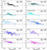 |
Fig. 7 Histogram shape parameter ξ (Eqs. (4) and (5)) calculated for the different NH bins in each region. The cases ξ> 0 and ξ< 0 correspond to the magnetic field oriented mostly parallel and perpendicular to the structure contours, respectively. For ξ ≈ 0 there is no preferred orientation. The displayed values of CHRO and XHRO were calculated from Eq. (6)and correspond to the grey dashed line in each plot. |
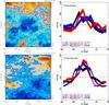 |
Fig. 8 Same as Fig. 3 for the two test regions located directly east (ChamEast) and south of Chamaeleon-Musca (ChamSouth). |
Fit of ξ vs. log 10(NH/ cm-2).
4.1.2. Histogram shape parameter ξ
The changes in the HROs are quantified using the histogram shape parameter ξ, defined as 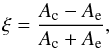 (4)where Ac is the area in the centre of the histogram (
 ) and Ae the area in the extremes of the histogram (
 and
and  ). The value of ξ, the result of the integration of the histogram over 45° ranges, is independent of the number of bins selected to represent the histogram if the bin widths are smaller than the integration range.
A concave histogram corresponding to B⊥ mostly aligned with NH contours would have ξ> 0. A convex histogram corresponding to B⊥ mostly perpendicular to NH contours would have ξ< 0. A flat histogram corresponding to no preferred relative orientation would have ξ ≈ 0.
The uncertainty in ξ, σξ, is obtained from 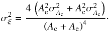 (5)The variances of the areas,
  and
and  , characterize the jitter of the histograms. If the jitter is large, σξ is large compared to | ξ | and the relative orientation is indeterminate. The jitter depends on the number of bins in the histogram, but ξ does not.
Figure 7 illustrates the change in ξ as a function of log 10(NH/ cm-2) of each bin. For most of the clouds, ξ is positive in the lowest and intermediate NH bins and negative or close to zero in the highest bins. The most pronounced changes in ξ from positive to negative are seen in Taurus, Chamaeleon-Musca, Aquila Rift, Perseus, and IC 5146.
The trend in ξ vs. log 10(NH/ cm-2) can be fit roughly by a linear relation ![Mathematical equation: \begin{equation} \label{eq:hrofit} \zeta = C_{{\rm HRO}}\,\left[\log_{10}\left(\nhd/{\rm cm}^{-2}\right) - X_{{\rm HRO}}\right]. \end{equation}](/articles/aa/full_html/2016/02/aa25896-15/aa25896-15-eq108.png) (6)The values of CHRO and XHRO in the regions analysed are summarized in Table 2. For the clouds with a pronounced change in relative orientation the slope CHRO is steeper than about − 0.5, and the value XHRO for the log 10(NH/ cm-2) at which the relative orientation changes from parallel to perpendicular is greater than about 21.7. Ophiuchus, Lupus, Cepheus, and Orion are intermediate cases, where ξ definitely does not go negative in the data, but seems to do so by extrapolation; these tend to have a shallower CHRO and/or a higher XHRO.
(6)The values of CHRO and XHRO in the regions analysed are summarized in Table 2. For the clouds with a pronounced change in relative orientation the slope CHRO is steeper than about − 0.5, and the value XHRO for the log 10(NH/ cm-2) at which the relative orientation changes from parallel to perpendicular is greater than about 21.7. Ophiuchus, Lupus, Cepheus, and Orion are intermediate cases, where ξ definitely does not go negative in the data, but seems to do so by extrapolation; these tend to have a shallower CHRO and/or a higher XHRO.
The least pronounced change in ξ is seen in CrA, where ξ is consistently positive in all bins, and the slope is very flat. We applied the HRO analysis to a pair of test regions (Fig. 8) with even lower NH values (log 10(NH/ cm-2) < 21.6; see also Fig. 11 below) located directly south and directly east of the Chamaeleon-Musca region. As in CrA, we find that B⊥ is mostly parallel to the NH contours, a fairly constant ξ, and no indication of predominantly perpendicular relative orientation.
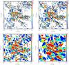 |
Fig. 9 Maps of the absolute value of the relative orientation angle, | φ |, in the Taurus region. These maps are produced after smoothing the input maps to beam FWHMs of 10′, 15′, 30′, and 60′ and then resampling the grid to sample each beam FWHM with the same number of pixels. The regions in red correspond to B⊥ close to perpendicular to NH structures. The regions in blue correspond to B⊥ close to parallel to NH structures. The black contour, corresponding to the NH value of the intermediate contour introduced in Fig. 3, provides a visual reference to the cloud structure. |
4.2. Comparisons with previous studies
The above trends in relative orientation between B⊥ and the NH contours in targeted MCs, where B⊥ tend to become perpendicular to the NH contours at high NH, agree with the results of the Hessian matrix analysis applied to Planck observations over the whole sky, as reported in Fig. 15 of Planck Collaboration Int. XXXII (2016).
Evidence for preferential orientations in sections of some regions included in this study has been reported previously. The Taurus region has been the target of many studies. Moneti et al. (1984) and Chapman et al. (2011) find evidence using infrared polarization of background stars for a homogeneous magnetic field perpendicular to the embedded dense filamentary structure. High-resolution submillimetre observations of intensity with Herschel find evidence of faint filamentary structures (“striations”), which are well correlated with the magnetic field orientation inferred from starlight polarization (Palmeirim et al. 2013) and perpendicular to the filament B211. Heyer et al. (2008) report a velocity anisotropy aligned with the magnetic field, which can be interpreted as evidence of the channeling effect of the magnetic fields. But the magnetic field in B211 and the dense filamentary structures are not measured directly. As described above, using Planck polarization we find that B⊥ is mostly aligned with the lowest NH contours (20.8 < log 10(NH/ cm-2) < 21.3; see also Planck Collaboration Int. XXXIII 2016), although the aligned structures do not correspond to the striations, which are not resolved at 10′ resolution. However, we also find that at higher NH the relative orientation becomes perpendicular.
Similar studies in other regions have found evidence of striations correlated with the starlight-inferred magnetic field orientation and perpendicular to the densest filamentary structures. The regions studied include Serpens South (Sugitani et al. 2011), which is part of Aquila Rift in this study, Musca (Pereyra & Magalhães 2004), and the Northern Lupus cloud (Matthews et al. 2014). By studying Planck polarization in larger regions around the targets of these previous observations, we show that a systematic change in relative orientation is the prevailing statistical trend in clouds that reach log 10(NH/ cm-2) ≳ 21.5.
 |
Fig. 10 HROs of the Taurus region after smoothing the input maps to beam FWHMs of 15′, 30′, and 60′, shown from left to right, respectively. |
5. Discussion
5.1. The relative orientation between B⊥ and NH structures
5.1.1. Spatial distribution of the HRO signal
The maps obtained using Eq. (2)characterize the relative orientation in each region, without assuming an organization of the NH structures in ridges or filaments; HROs basically just sample the orientation of NH contours. However, the resulting maps of the relative orientation angle, shown for the Taurus region in Fig. 9, reveal that the regions that are mostly oriented parallel or perpendicular to the field form continuous patches, indicating that the HRO signal is not only coming from variations in the field or the NH contours at the smallest scales in the map.
HRO analysis on larger scales in a map can be achieved by considering a larger vicinity of pixels for calculating the gradient ∇τ353. This operation is equivalent to calculating the next-neighbour gradient on a map first smoothed to the scale of interest. The results for relative orientation after smoothing to resolutions of 15′, 30′, and 60′ are illustrated for the Taurus region in Fig. 9. Figure 10 shows that the corresponding HROs have a similar behaviour for the three representative NH values. These results confirm that the preferred relative orientation is not particular to the smallest scales in the map, but corresponds to coherent structures in NH.
A study of the preferred orientation for the whole cloud would be possible by smoothing the column density and polarization maps to a scale comparable to the cloud size. The statistical significance of such a study would be limited to the number of clouds in the sample and would not be directly comparable to previous studies of relative orientation of clouds, where elongated structures were selected to characterize the mean orientation of each cloud (Li et al. 2013).
5.1.2. Statistical significance of the HRO signal
Our results reveal a systemic change of ξ with NH, suggesting a systematic transition from magnetic field mostly parallel to NH contours in the lowest NH bins to mostly perpendicular in the highest NH bins of the clouds studied. The statistical significance of this change can in principle be evaluated by considering the geometrical effects that influence this distribution. In Appendix C.1, using simulations of Q and U maps, we eliminate the possibility that this arises from random magnetic fields, random spatial correlations in the field, or the large scale structure of the field. In Appendix C.2 we simply displace the Q and U maps spatially and repeat the analysis, showing that the systemic trend of ξ vs. NH disappears for displacements greater than 1°.
Using a set of Gaussian models, Planck Collaboration Int. XXXII (2016) estimated the statistical significance of this transition in terms of the relative orientation between two vectors in 3D and their projection in 2D. As these authors emphasized, two vectors that are close to parallel in 3D would be projected as parallel in 2D for almost all viewing angles for which the projections of both vectors have a non-negligible length, but on the other hand, the situation is more ambiguous seen in projection for two vectors that are perpendicular in 3D, because they can be projected as parallel in 2D depending on the angle of viewing. The quantitative effects are illustrated by the simulations in Appendix C.3, where we consider distributions of vectors in 3D that are mostly parallel, mostly perpendicular, or have no preferred orientation. The projection tends to make vector pairs look more parallel in 2D, but the distribution of relative orientations in 2D is quite similar though not identical to the distribution in 3D. In particular, the signal of perpendicular orientation is not erased and we can conclude that two projected vectors with non-negligible lengths that are close to perpendicular in 2D must also be perpendicular in 3D. This would apply to the mostly perpendicular orientation for the highest bin of NH in the Taurus region.
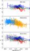 |
Fig. 11 Histogram shape parameter ξ (Eqs. (4) and (5)) calculated for the different NH bins in each region. Top: relative orientation in synthetic observations of simulations with super-Alfvénic (blue), Alfvénic (green), and sub-Alfvénic (red) turbulence, as detailed in Soler et al. (2013). Middle: relative orientation in the regions selected from the Planck all-sky observations, from Fig. 7. The blue data points correspond to the lowest NH regions (CrA and the test regions in Fig. 8, ChamSouth and ChamEast) and the orange correspond to the rest of the clouds. Bottom: comparison between the trends in the synthetic observations (in colours) and the regions studied (grey). The observed smooth transition from mostly parallel (ξ> 0) to perpendicular (ξ< 0) is similar to the transition in the simulations for which the turbulence is Alfvénic or sub-Alfvéic. |
5.2. Comparison with simulations of MHD turbulence
As a complement to observations, MHD simulations can be used to directly probe the actual 3D orientation of the magnetic field B with respect to the density structures. The change in the relative orientation with NH was previously studied in MHD simulations using the inertia matrix and the HRO analysis (Hennebelle 2013; Soler et al. 2013). Soler et al. (2013) showed that in 3D, the change in the relative orientation is related to the degree of magnetization. If the magnetic energy is above or comparable to the kinetic energy (turbulence that is sub-Alfvénic or close to equipartition), the less dense structures tend to be aligned with the magnetic field and the orientation progressively changes from parallel to perpendicular with increasing density. In the super-Alfvénic regime, where the magnetic energy is relatively low, there appears to be no change in relative orientation with increasing density, with B and density structures being mostly parallel.
Soler et al. (2013) describe 2D synthetic observations of the MHD simulations. The synthetic observations are produced by integrating the simulation cubes along a direction perpendicular to the mean magnetic field and assuming a homogeneous dust grain alignment efficiency ϵ = 1.0. The angular resolution of the simulation is obtained by assuming a distance d = 150 pc and convolving the projected map with a Gaussian beam of 10′ full width at half maximum (FWHM). The trends in the relative orientation with NH seen in 3D are also seen using the these 2D synthetic observations. Given that sub-Alfvénic or close to Alfvénic turbulence does not significantly disturb the well-ordered mean magnetic field, the orientation of B perpendicular to the iso-density contours is projected well for lines of sight that are not close to the mean magnetic field orientation. In contrast, the projected relative orientation produced by super-Alfvénic turbulence does not necessarily reflect the relative orientation in 3D as a result of the unorganized field structure.
The direct comparison between the HROs of the regions in this study and of the synthetic observations is presented in Fig. 11. The trends in the relative orientation parameter, ξ, show that the simulation with super-Alfvénic turbulence does not undergo a transition in relative orientation from parallel to perpendicular for log 10(NH/ cm-2) < 23. In contrast, most of the observed clouds show a decrease in ξ with increasing NH, close to the trends seen from the simulations with Alfvénic or sub-Alfvénic turbulence for log 10(NH/ cm-2) < 23. Furthermore, XHRO, the value of log 10(NH/ cm-2) where ξ goes through zero, is near 21.7, which is consistent with the behaviour seen in the simulations with super-Alfvénic or Alfvénic turbulence. Given that the physical conditions in the simulations (σv = 2.0 km s-1 and n = 500 cm-3) are typical of those in the selected regions (σv∥ is given in Table D.1), the similarities in the dependence of ξ on NH suggest that the strength of the magnetic field in most of the regions analysed would be about the same as the mean magnetic fields in the Alfvénic and sub-Alfvénic turbulence simulations, which are 3.5 and 11 μG, respectively. However, more precise estimates of the magnetic field strength coming directly from the HROs would require further sampling of the magnetization in the MHD simulations and detailed modelling of the effects of the line-of-sight integration.
Indirectly, the presence of a NH threshold in the switch in preferred relative orientation between B⊥ and the NH structures hints that gravity plays a significant role. By contrast, for the regions with low average NH (i.e., CrA and the two test regions; Fig. 11), there is little change in ξ and certainly no switch in the preferred relative orientation to perpendicular.
5.3. Physics of the relative orientation
The finding of dense structures mostly perpendicular to the magnetic field (and the small mass-to-flux ratios discussed in Appendix D.4) suggests that the magnetic field in most of the observed regions is significant for the structure and dynamics. However, discerning the underlying geometry is not obvious. As one guide, a frozen-in and strong interstellar magnetic field would naturally cause a self-gravitating, static cloud to become oblate, with its major axis perpendicular to the field lines, because gravitational collapse would be restricted to occurring along field lines (Mouschovias 1976a,b). In the case of less dense structures that are not self-gravitating, the velocity shear can stretch matter and field lines in the same direction, thereby producing aligned structures, as discussed in Hennebelle (2013) and Planck Collaboration Int. XXXII (2016).
If the MCs are isolated entities and the magnetic field is strong enough to set a preferred direction for the gravitational collapse, the condensations embedded in the cloud are not very likely to have higher column densities than their surroundings (Nakano 1998). This means that the formation of dense substructures, such as prestellar cores and stars, by gravitational collapse would be possible only if the matter decouples from the magnetic field. This is possible through the decoupling between neutral and ionized species (ambipolar diffusion, Mouschovias 1991; Li & Houde 2008) or through removal of magnetic flux from clouds via turbulent reconnection (Lazarian & Vishniac 1999; Santos-Lima et al. 2012).
Alternatively, if we regard MCs not as isolated entities but as the result of an accumulation of gas by large-scale flows (Ballesteros-Paredes et al. 1999; Hartmann et al. 2001; Koyama & Inutsuka 2002; Audit & Hennebelle 2005; Heitsch et al. 2006), the material swept up by colliding flows may eventually form a self-gravitating cloud. If the magnetic field is strong the accumulation of material is favoured along the magnetic field lines, thus producing dense structures that are mostly perpendicular to the magnetic field. The inflow of material might eventually increase the gravitational energy in parts of the cloud, thereby producing supercritical structures such as prestellar cores.
For supersonic turbulence in the ISM and MCs, density structures can be formed by gas compression in shocks. If the turbulence is strong with respect to the magnetic field (super-Alfvénic), gas compression by shocks is approximately isotropic; because magnetic flux is frozen into matter, field lines are dragged along with the gas, forming structures that tend to be aligned with the field. If the turbulence is weak with respect to the magnetic field (sub-Alfvénic), the fields produce a clear anisotropy in MHD turbulence (Sridhar & Goldreich 1994; Goldreich & Sridhar 1995; Matthaeus et al. 2008; Banerjee et al. 2009) and compression by shocks that is favored to occur along the magnetic field lines, creating structures perpendicular to the field. The cold phase gas that constitutes the cloud receives no information about the original flow direction because the magnetic field redistributes the kinetic energy of the inflows (Heitsch et al. 2009; Inoue & Inutsuka 2009; Burkhart et al. 2014). This seems to be the case in most of the observed regions, where the mostly perpendicular relative orientation between the magnetic field and the high column density structures is an indication of the anisotropy produced by the field.
The threshold of log 10(NH/ cm-2) ≈ 21.7 above which the preferential orientation of B⊥ switches to being perpendicular to the NH contours is intriguing. Is there a universal threshold column density that is independent of the particular MC environment and relevant in the context of star formation? In principle, this threshold might be related to the column density of filaments at which substructure forms, as reported in an analysis of Herschel observations (Arzoumanian et al. 2013), but the Planck polarization observations leading to B⊥ do not fully resolve such filamentary structures. In principle, this threshold might also be related to the column density at which the magnetic field starts scaling with density, according to the Zeeman effect observations of B∥ (Fig. 7 in Crutcher 2012). However, establishing such relationships requires further studies with MHD simulations to identify what densities and scales influence the change in relative orientation between B⊥ and NH structures and to model the potential imprint in B∥ observations and in B⊥ observations to be carried out at higher resolution.
5.4. Effect of dust grain alignment
Throughout this study we assume that the polarized emission observed by Planck at 353 GHz is representative of the projected morphology of the magnetic field in each region; i.e., we assume a constant dust grain alignment efficiency (ϵ) that is independent of the local environment. Indeed, observations and MHD simulations under this assumption (Planck Collaboration Int. XIX 2015; Planck Collaboration Int. XX 2015) indicate that depolarization effects at large and intermediate scales in MCs might arise from the random component of the magnetic field along the line of sight. On the other hand, the sharp drop in the polarization fraction at NH> 1022 cm-2 (reported in Planck Collaboration Int. XIX 2015), when seen at small scales, might be interpreted in terms of a decrease of ϵ with increasing column density (Matthews et al. 2001; Whittet et al. 2008).
A leading theory for the process of dust grain alignment involves radiative torques by the incident radiation (Lazarian & Hoang 2007; Hoang & Lazarian 2009; Andersson 2015). A critical parameter for this mechanism is the ratio between the dust grain size and the radiation wavelength. As the dust column density increases, only the longer wavelength radiation penetrates the cloud and the alignment decreases. Grains within a cloud (without embedded sources) should have lower ϵ than those at the periphery of the same cloud. There is evidence for this from near-infrared interstellar polarization and submillimetre polarization along lines of sight through starless cores (Jones et al. 2015), albeit on smaller scales and higher column densities than considered here. If ϵ inside the cloud is very low, the observed polarized intensity would arise from the dust in the outer layers, tracing the magnetic field in the “skin” of the cloud. Then the observed orientation of B⊥ is not necessarily correlated with the column density structure, which is seen in total intensity, or with the magnetic field deep in the cloud.
Soler et al. (2013) presented the results of HRO analysis on a series of synthetic observations produced using models of how ϵ might decrease with increasing density. They showed that with a steep decrease there is no visible correlation between the inferred magnetic field orientation and the high-NH structure, corresponding to nearly flat HROs.
The HRO analysis of MCs carried out here reveals a correlation between the polarization orientation and the column density structure. This suggests that the dust polarized emission samples the magnetic field structure homogeneously on the scales being probed at the resolution of the Planck observations or, alternatively, that the field deep within high-NH structures has the same orientation of the field in the skin.
6. Conclusions
We have presented a study of the relative orientation of the magnetic field projected on the plane of the sky (B⊥), as inferred from the Planck dust polarized thermal emission, with respect to structures detected in gas column density (NH). The relative orientation study was performed by using the histogram of relative orientations (HRO), a novel statistical tool for characterizing extended polarization maps. With the unprecedented statistics of polarization observations in extended maps obtained by Planck, we analyze the HRO in regions with different column densities within ten nearby molecular clouds (MCs) and two test fields.
In most of the regions analysed we find that the relative orientation between B⊥ and NH structures changes systematically with NH from being parallel in the lowest column density areas to perpendicular in the highest column density areas. The switch occurs at log 10(NH/ cm-2) ≈ 21.7. This change in relative orientation is particularly significant given that projection tends to produce more parallel pseudo-vectors in 2D (the domain of observations) than exist in 3D.
The HROs in these MCs reveal that most of the high NH structures in each cloud are mostly oriented perpendicular to the magnetic field, suggesting that they may have formed by material accumulation and gravitational collapse along the magnetic field lines. According to a similar study where the same method was applied to MHD simulations, this trend is only possible if the turbulence is Alfvénic or sub-Alfvénic. This implies that the magnetic field is significant for the gas dynamics on the scales sampled by Planck. The estimated mean magnetic field strength is about 4 and 12 μG for the case of Alfvénic and sub-Alfvénic turbulence, respectively.
We also estimate the magnetic field strength in the MCs studied using the DCF and DCF+SF methods. The estimates found seem consistent with the above values from the HRO analysis, but given the assumptions and systematic effects involved, we recommend that these rough estimates be treated with caution. According to these estimates the analysed regions appear to be magnetically sub-critical. This result is also consistent with the conclusions of the HRO analysis. Specific tools, such as the DCF and DCF+SF methods, are best suited to the scales and physical conditions in which their underlying assumptions are valid. The study of large polarization maps covering multiple scales calls for generic statistical tools, such as the HRO, for characterizing their properties and establishing a direct relation to the physical conditions included in MHD simulations.
The study of the structure on smaller scales is beyond the scope of this work, however, the presence of gravitationally bound structures within the MCs, such as prestellar cores and stars, suggests that the role of magnetic fields is changing on different scales. Even if the magnetic field is important in the accumulation of matter that leads to the formation of the cloud, effects such as matter decoupling from the magnetic field and the inflow of matter from the cloud environment lead to the formation of magnetically supercritical structures on smaller scales. Further studies will help to identify the dynamical processes that connect the MC structure with the process of star formation.
Appendix A: Selection of data
The HRO analysis is applied to each MC using common criteria for selecting the areas in which the relative orientation is to be assessed.
Appendix A.1: Gradient mask
The dust optical depth, τ353, observed in each region, can be interpreted as  (A.1)where
  is the optical depth of the MC,
  is the optical depth of the diffuse regions behind and/or in front of the cloud (background/foreground), and δτ353 the noise in the optical depth map with variance
  .
.
The gradient of the optical depth can be then written as  (A.2)We quantify the contribution of the background/foreground and the noise,
  , by evaluating ∇τ353 in a reference field with lower submillimetre emission. Given that the dominant contribution to the background/foreground gradient would come from the gradient in emission from the Galactic plane, for each of the regions analysed we chose a reference field of the same size at the same Galactic latitude and with the lowest average NH in the corresponding latitude band. We compute the average of the gradient norm in the reference field,
  , and use this value as a threshold for selecting the regions of the map where ∇τ353 carries significant information about the structure of the cloud. We note that this threshold includes a contribution from the noise ∇δτ353. The HROs presented in this study correspond to regions in each field where
  .
.
Appendix A.2: Polarization mask
The total Stokes parameters Q and U measured in each region can be interpreted as  (A.3)where Qmc and Umc correspond to the polarized emission from the MC, Qbg and Ubg correspond to the polarized emission from the diffuse background/foreground, and δQ and δU are the noise contributions to the observations, such that the variances
  and
and  .
.
As in the treatment of the gradient, we estimate the contributions of the background/foreground polarized emission and the noise using the rms of the Stokes parameters in the same reference field,  and
and  . The HROs presented in this study correspond to pixels in each region where
  or
or  . The “or” conditional avoids biasing the selected values of polarization. This first selection criterion provides a similar sample to the alternative coordinate-independent criterion
  . This first criterion aims to distinguish between the polarized emission coming from the cloud and the polarized emission coming from the background/foreground estimated in the reference regions.
Additionally, as a second criterion, our sample is restricted to polarization measurements where | Q | > 3σQ or | U | > 3σU. This aims to select pixels where the uncertainty in the polarization angle is smaller than the size of the angle bins used for the constructions of the HRO (Serkowski 1958; Montier et al. 2015). In terms of the total polarized intensity,  , and following Eqs. (B.4) and (B.5) in Planck Collaboration Int. XIX (2015), the second criterion corresponds to P/σP> 3 and uncertainties in the polarized orientation angle σψ< 10°.
The fractions of pixels considered in each region, after applying the selection criteria described above, are summarized in Table A.1. The largest masked portions of the regions correspond to the gradient mask, which selects mostly those areas of column density above the mean column density of the background/foreground  . The polarization mask provides an independent criterion that is less restrictive. The intersection of these two masks selects the fraction of pixels considered for the HRO analysis.
Selection of data.
Appendix B: Construction of the histogram of relative orientations and related uncertainties
The HROs were calculated for 25 column density bins having equal numbers of selected pixels (10 bins in two regions with fewer pixels, CrA and IC 5146). For each of these HROs we use 12 angle bins of width 15° (see Sect. 4.1.1).
Appendix B.1: Calculation of ∇τ353 and the uncertainty of its orientation
The optical depth gradient (∇τ353) is calculated by convolving the τ353 map with a Gaussian derivative kernel (Soler et al. 2013), such that ∇τ353 corresponds to  (B.1)where Gx and Gy are the kernels calculated using the x- and y-derivatives of a symmetric two-dimensional Gaussian function. The orientation of the iso-τ353 contour is calculated from the components of the gradient vector,
  (B.2)Because the calculation of the gradient through convolution is a linear operation, the associated uncertainties can be calculated using the same operation,so that
  (B.3)from which we obtain the
  and
and  .
.
The standard deviation of the angle θ can be written as  (B.4)which corresponds to
  (B.5)In the application discussed here, the standard deviations in the τ353 map within the selected areas are much less than a few percentage points, so their effect on the estimate of the orientation of the gradient is negligible.
Appendix B.2: Uncertainties affecting the characterization of relative orientations within MCs
Appendix B.2.1: Uncertainties in the construction of the histogram
To estimate the uncertainty associated with the noise in Stokes Q and U, we produce 1000 noise realizations, Qr and Ur, using Monte Carlo sampling. We assume that the errors are normally distributed and are centred on the measured values Q and U with dispersions σQ and σU (Planck Collaboration II 2014; Planck Collaboration VI 2014; Planck Collaboration V 2014; Planck Collaboration VIII 2014). Given that σQU is smaller than  and
and  , it is justified to generate Qr and Ur independently of each other. We then introduce Qr and Ur in the analysis pipeline and compute the HRO using the corresponding τ353 map in each region. The results, presented in Fig. B.1 for the Taurus region, show that the noise in Q and U does not critically affect the shape of the HROs or the trend in ξ. Together, the low noise in the maps of τ353 and the selection criteria for the polarization measurements ensure that the HRO is well determined.
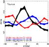 |
Fig. B.1 HROs in the Taurus region that correspond to the indicated NH bins. The plotted values are obtained using the original τ353 map at 10′ resolution and maps of the Stokes parameters Qr and Ur, which correspond to 1000 random noise realizations. Each realization is generated using a Gaussian probability density function centred on the measured values Q and U with variances |


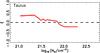 |
Fig. B.2 Histogram shape parameter, ξ, as a function of log 10(NH/ cm-2) in the Taurus region. The values are obtained using the τ353 map at 10′ resolution and maps of the Stokes parameters Qr and Ur that correspond to 1000 random-noise realizations. Each realization is generated using a Gaussian probability density function centred on the measured values Q and Uwith variances |
Another source of uncertainty in the HRO resides in the histogram binning process. The variance in the kth histogram bin is given by  (B.6)where hk is the number of samples in the kth bin, and htot is the total number of samples.
Of the two independent sources of uncertainty above, we find that the largest contribution comes from the binning process, so that these are the ones shown as the shaded uncertainty ranges in all figures of HROs, for example for Taurus in Fig. 3. Because of the large number of samples in each histogram bin, the uncertainties in the HRO do not significantly affect the results of this study.
Appendix B.2.2: Uncertainties in the histogram shape parameter ξ
As in the case of the HRO, the uncertainty in ξ, as defined in Eq. (4), can be quantified using the random realizations introduced in the previous section. Figure B.2 shows the dependence of ξ on log 10NH obtained using Qr and Ur for the Taurus region. The small variations around the trend line indicate that the uncertainties in Q and U do not significantly affect the trends discussed in this study, as expected from the behaviour of the histograms presented in Fig. B.1. The main source of uncertainty in the estimation of ξ is related to the histogram binning, characterized by the error bars calculated using Eq. (5). As seen in Fig. 7 and reproduced in Fig. C.1, these are much larger than the dispersion of the values of ξ in Fig. B.2.
Appendix C: Statistical significance of the HRO signal
Appendix C.1: A product of chance?
To investigate various potential sources of the signal found in the HROs we use the τ353 map at 10′ resolution in each region in combination with Q and U maps that are produced with different recipes, each with 1000 realizations.
To eliminate random fields, we use Q and U maps produced with a random realization of ψ with a uniform distribution and with unit-length polarization pseudo-vectors. The results of this numerical experiment are shown in Fig. C.1 for the Taurus region. For each of the 1000 realizations, we join the values at each NH bin to show the trend lines in order to compare with the lines in Fig. 7.
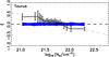 |
Fig. C.1 Histogram shape parameter, ξ, as a function of log 10(NH/ cm-2) in the Taurus region. Blue lines join the ξ values obtained using the τ353 map at 10′ resolution and each of 1000 random realizations of Q and U maps corresponding to a uniform distribution of ψ. Results in black and grey are from the analysis of the Planck data, as reported in Fig. 7. |
To eliminate the large-scale magnetic field as the source we use Q and U maps produced with random realizations of ψ with a Gaussian distribution and unit-length polarization pseudo-vectors. The polarization angle distribution is centred at ψ0 = 0° with a standard deviation ςψ = 45°. The results of this numerical experiment are shown in Fig. C.2 for the Taurus region.
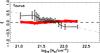 |
Fig. C.2 Like Fig. C.1 but for values of ξ (red) obtained using 1000 random realizations of Q and U maps corresponding to a Gaussian distribution of ψ centred on ψ0 = 0° and with standard deviation ςψ = 45°. |
To eliminate random spatial correlations, we use Q and U maps produced from random realizations with a power spectrum P(k) ∝ kαm. For the spectral indices we adopted, αm = −1.5, − 2.5, and − 3.5, correlations are introduced in the orientation of the polarization pseudo-vectors that are independent of the structure of matter. This test evaluates the statistical significance of the random sampling of spatial correlations in the magnetic field implied when we calculate the HROs in a finite region of the sky. The results of this numerical experiment are shown in Fig. C.3 for the Taurus region.
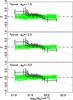 |
Fig. C.3 Like Fig. C.1 but for values of ξ (green) obtained using 1000 random realizations of Q and U maps corresponding to a power spectrum P(k) ∝ kαm, with αm = −1.5, − 2.5, and − 3.5. |
The results of these numerical experiments show that the trends with NH found in the HROs and ξ do not arise by chance from these potential sources.
Appendix C.2: A product of random correlations in the polarization maps?
The random realizations of the magnetic field presented above are useful for characterizing the behaviour of ξ. However, they are bound to produce very different statistics compared to those in the real observations. In reality the orientations of B⊥ have some non-trivial correlation structure in the map. In principle, the difference in the HROs might be due to the different correlations of the observed B⊥ and of the random realizations of B⊥.
To evaluate whether the signal present in the HROs arises from an actual physical relationship between B⊥ and τ353, we introduce randomness by shifting the Stokes Q and U maps with respect to the τ353 map and then calculate the corresponding HROs and ξ as a function of log 10(NH/ cm-2). The intrinsic statistical properties of the two maps are unchanged because the two maps are unchanged, only shifted.
If the trend in ξ as a function of log 10(NH/ cm-2) were arising randomly, these trends would be unchanged even for significant shifts. Instead the results of this experiment, illustrated in Fig. C.4 for the Taurus region, show that the trends tend to disappear with increasing values of the size of the shift. For shifts of about 1°, the correlation between the magnetic field and the matter is still present, as expected from the results presented in Fig. 10, but for larger shifts the correlation is lost and the trend does not survive. Over the many MCs studied, the nature of the trends at large shifts appears to be random.
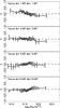 |
Fig. C.4 Histogram shape parameter, ξ, as a function of log 10(NH/ cm-2) calculated from the τ353 map at 10′ resolution in the Taurus region and the Stokes Q and U maps shifted in Galactic longitude and latitude by the values indicated, for Δl and Δb, respectively. |
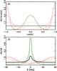 |
Fig. C.5 Normalized distributions of relative orientations of random vectors in 3D (top) and of their projections in 2D (bottom). The curves correspond to mostly perpendicular vectors (red), uniform distribution of relative orientations (black), and mostly parallel vectors (green). The solid, dashed, and dotted lines correspond to dispersions of the relative orientation angle ςα = 18°, 36°, and 72°, respectively. |
Appendix C.3: Projection effects
We evaluate the statistical significance of the relative orientation between B⊥ and ∇τ353 by considering the distribution of relative orientations between two vectors in 3D space compared to the distribution of relative orientation between their projections in 2D.
The projection of a vector v onto a plane normal to the unit vector  can be written as
  (C.1)
(C.1)
Consider two unit vectors in 3D, v1 and v2, separated by an angle α, such that  (C.2)The angle β between the projections of these two vectors onto a plane normal to , u1, and u2, can be written as
  (C.3)Given a particular distribution of angles between the vectors v1 and v2, this expression, which is solved numerically, is useful for evaluating the resulting distribution of angles between the projected vectors u1 and u2. Without any loss of generality, we can assume that v1 is oriented along the axis of a spherical coordinate system, such that
  , and that v2 is oriented at polar angle θ and azimuth φ, such that
  . Then, we can simulate a distribution of cosα by simulating a distribution of cosθ and generating φ with a uniform distribution.
We thus generate a set of vectors v2 that follow a particular distribution of cosα. We choose three examples: a uniform distribution of relative orientation between v2 and v1, v2 vectors that are mostly parallel to v1, and v2 vectors that are mostly perpendicular to v1. The last two are Gaussian distributions centred at cosα = 0 (for mostly parallel) or cosα = ± 1 (for mostly perpendicular, given the periodicity of α) with a dispersion ςα. These distributions are shown in the top panel of Fig. C.5 for three values of ςα.
Using Eq. (C.3)we calculate the distribution of the angles between the projected vectors and the results are shown in the bottom panel of Fig. C.5. Projection generally tends to make vector pairs look more parallel in 2D than they are in 3D, regardless of the orientation in 3D, in agreement with the results of the Gaussian models presented in Planck Collaboration Int. XXXII (2016). Nevertheless, the distribution of relative orientations in 2D is qualitatively similar (though not identical) to the distribution in 3D. In particular, the signature of perpendicular orientation is not erased. We conclude that the observation in 2D of B⊥ close to perpendicular to the column density structures is a direct indicator of the perpendicular configuration of B with respect to the density structures in 3D. In contrast, the parallel alignment of B⊥ with the structure, or no signs of preferential orientation, while suggestive of parallel orientation in 3D, does not unambiguously rule out the presence of some close-to-perpendicular orientations within the distribution in 3D.
Appendix D: Alternative estimates of magnetic field strength
Given the historic importance of the DCF method (Davis 1951; Chandrasekhar & Fermi 1953) and the related DCF+SF method (Hildebrand et al. 2009), we have used them to estimate the magnetic field strength in each region. We also evaluated the mass-to-flux ratio, which is important in investigating the stability against gravitational collapse. We now provide a critical assessment of the applicability of these results.
Appendix D.1: Davis-Chandrasekhar-Fermi method
The DCF method estimates the strength of B⊥ in a region using the dispersion of the polarization angles ςψ. Assuming that the magnetic field is frozen into the gas and that the dispersion of the B⊥ orientation angles (or equivalently ςψ) is due to transverse incompressible Alfvén waves, then  (D.1)where σv∥ is the dispersion of the radial velocity of the gas (Appendix D.3) and ρ the gas mass density.
We calculate ςψ directly from Stokes Q and U using  (D.2)and
  (D.3)where ⟨... ⟩ denotes an average over the selected pixels in each map (Planck Collaboration Int. XIX 2015).
Magnetic properties of the selected regions.
Appendix D.2: Davis-Chandrasekhar-Fermi plus structure function method
As described by Hildebrand et al. (2009), the DCF+SF method characterizes the magnetic field dispersion about local structured fields by considering the difference in angle, Δψ(ℓ) = ψ(x)−ψ(x+ℓ), between pairs of B⊥ vectors separated by displacements ℓ in the plane of the sky. Assuming that the angle differences are statistically isotropic (i.e., they depend only on ℓ = | ℓ | and not on the orientation of ℓ), they can binned by distance, ℓ. From the N(ℓ) pairs of B⊥ vectors for that bin, the square of the second-order structure function is ![Mathematical equation: \appendix \setcounter{section}{4} \begin{equation} \label{eq:strucfunc} S^{2}_{2}(\ell) = \left< [\Delta\psi(\vec{x},\ell)]^{2} \right>_{x} = \left<\frac{1}{N(\ell)}\sum\limits_{i=1}^{N(\ell)} (\Delta\psi_{x,i})^{2} \right>_{x} , \end{equation}](/articles/aa/full_html/2016/02/aa25896-15/aa25896-15-eq237.png) (D.4)as introduced by Kobulnicky et al. (1994) and Falceta-Gonçalves et al. (2008). In terms of the Stokes parameters, each term in the sum can be written
(D.4)as introduced by Kobulnicky et al. (1994) and Falceta-Gonçalves et al. (2008). In terms of the Stokes parameters, each term in the sum can be written  (D.5)where the subscripts x and i represent the central and displaced positions, respectively.
Hildebrand et al. (2009) assume that B(x) is composed of a large-scale structured field, B0(x), and a random component, Br(x), which are statistically independent of each other. Assuming that B0(x) is a smoothly varying quantity, its contribution to  should increase in proportion to ℓ2 for distances that are much smaller than the scales at which B0 itself fluctuates. Additionally, assuming that turbulence occurs on scales that are small enough to completely decorrelate Br for the range of scales probed by the displacements ℓ, Hildebrand et al. (2009) derived the approximation
  (D.6)where the two terms on the right-hand side give the contributions from the random and large-scale magnetic fields, respectively. These assumptions are not necessarily valid for the range of scales in the Planck data.
Hildebrand et al. (2009) used Eq. (D.6)to estimate b2 as the intercept and then related b to the ratio of the random to the large-scale magnetic field strength, both projected onto the plane of the sky, through 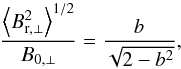 (D.7)where
  stands for the root mean square (rms) variations about the large-scale magnetic field, B0, ⊥. The same assumptions that result in Eq. (D.1)– i.e., considering only incompressible and isotropic turbulence, magnetic fields frozen into the gas, and dispersion of the B⊥ orientation originating in transverse incompressible Alfvén waves – lead to
 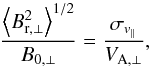 (D.8)where
 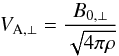 (D.9)is the speed of the transverse incompressible Alfvén waves. Combining Eqs. (D.7) – (D.9)results in
 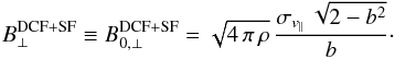 (D.10)
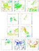 |
Fig. D.1 Line-of-sight centroid velocity v∥ maps inferred from CO emission (Dame et al. 2001). Areas shown have sufficient S/N in the polarization observations (second polarization criterion in Appendix A.2) for the DCF and DCF+SF analyses and lie in the range − 10 <v∥/ (km s-1) < 10. |
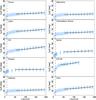 |
Fig. D.2 Structure function S2(ℓ) calculated from the Q and U maps of the selected regions following Eq. (D.4). The black lines indicate the fits given by Eq. (D.6). The vertical dashed line marks the common 10′ resolution of the data used in the analysis; the data are correlated for low values of ℓ causing the drop in S2(ℓ). |
Appendix D.3: Calculation
The estimates of velocity dispersion σv∥ and mass density ρ are the same in the two methods (DCF and DCF+SF).
We obtain σv∥ from the most complete CO emission-line survey of the Milky Way currently available, that of Dame et al. (2001). This data set consists of 488 000 spectra that beam-sample (1/8°) a set of MCs and the Galactic plane over a strip from 4° to 10° wide in latitude. We find that material in the MCs has centroid velocities in the range − 10 <v∥/ (km s-1) < 10 in the first moment map. Furthermore, for the calculations below, we need to select pixels with sufficient S/N in the polarization observations and so use the second criterion described in Appendix A.2. This combination of cuts selects the areas illustrated in Fig. D.1. Over these areas we calculate the average of the velocity dispersion from the second moment map and use this value as σv∥. This is tabulated along with other properties in Table D.1.
The mass density, ρ = μnmp, is the product of the proton mass, mp, the mean molecular weight per hydrogen molecule, μ = 2.8, and the mean number density, n. We require a value of n, which for the discussions here we approximate to be 100 cm-3. This is a typical value for MCs (Draine 2011) and in rough agreement with the column densities and cloud sizes presented in Table 1. In practice, n varies from one cloud to the next, and its estimation involves the assumption of a particular cloud geometry, resulting in additional uncertainties that are not considered in this study.
For the DCF method, the dispersion of the orientation angle ςψ corresponds to the centred second moment of the ψ distribution evaluated in pixels within the selected region. Following the analysis presented in Planck Collaboration Int. XIX (2015) for  , the variance on ςψ can be expressed as
 ![Mathematical equation: \appendix \setcounter{section}{4} \begin{equation} \label{eq:varsigmadebiassigma} \sigma^{2}_{\varsigma_{\psi}} = \frac{1}{N^{2}\varsigma^{2}_{\psi}}\left[\left(\sum\limits_{i=1}^{N}\varsigma_{i}\right)^{2}\sigma^{2}_{\psi} + \sum\limits_{i=1}^{N}\varsigma^{2}_{i}\sigma^{2}_{\psi_{i}} \right] , \end{equation}](/articles/aa/full_html/2016/02/aa25896-15/aa25896-15-eq264.png) (D.11)where ψi and σψi are the orientation angle and uncertainty for each polarization pseudo-vector, N is the number of ψ measurements, ςi = ψi−⟨ψ⟩, and ⟨ψ⟩ is the average orientation angle in each region. Like other quadratic functions,
(D.11)where ψi and σψi are the orientation angle and uncertainty for each polarization pseudo-vector, N is the number of ψ measurements, ςi = ψi−⟨ψ⟩, and ⟨ψ⟩ is the average orientation angle in each region. Like other quadratic functions,  is biased positively when noise is present, leading to an overestimation of this quantity. However, given that we limit our analysis to polarization measurements with high S/N and that the uncertainties in σv∥ are considerably larger, the bias correction does not have a significant effect on our estimates. We apply Eq. (D.1)to estimate
  and propagate the errors to obtain the values listed in Table D.1.
For the DCF+SF method, to estimate the parameter b, we first calculate  for each of the regions. The resolution of the data used is 10′. We evaluate in steps of
  for lags 0′
  and in steps of
  for lags 40′ <ℓ< 200′. For each considered lag ℓ, Δψx,i is evaluated pixel by pixel, considering all the pixels located in an annulus with radius ℓ. The term Δψx,i is only considered in the calculation of if there are at least three pixels in the annulus. As anticipated, the model from Eq. (D.6)does not agree with the data on all sampled scales, so the range of scales considered is limited to ℓ above the resolution of the data and between 50′ and 200′, where the behaviour of is approximately linear in ℓ2. We then make a linear fit of using ℓ2 as the independent variable and estimate the value of b and its uncertainty, σb. The results are plotted in Fig. D.2.
Using the calculated b values6, we apply Eq. (D.10)to estimate  , and the results are listed in Table D.1. As expected, the DCF+SF method produces estimates of B⊥ that are about twice as large as those obtained with the DCF method. However, it is worth noting that because of the discrepancy between the model and the observations, the value of b depends on the selected ℓ-range and so propagates into a different value of .
Appendix D.4: Mass-to-flux ratios
The critical value for the mass that can be supported against gravity by a magnetic flux Φ can be estimated to first order for a uniform disk from (M/ Φ)crit≡1 / (2πG1 / 2) (Nakano & Nakamura 1978). The precise value of the right-hand side changes for different geometries (e.g., Spitzer 1968; McKee et al. 1993). Stability can be assessed using 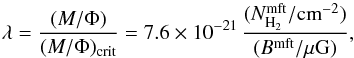 (D.12)where
  and Bmft are the H2 column density and magnetic field strength along a magnetic flux tube (Crutcher et al. 2004). A cloud is supercritical and prone to collapse under its own gravity, when λ> 1; otherwise, when λ< 1, the cloud is sub-critical, magnetically supported against gravitational collapse.
What is observable is λobs, in which  is replaced by NH2/B⊥. We evaluate λobs by combining the value of ⟨NH2⟩ computed from the integrated CO line emission and the conversion factor XCO = (1.8 ± 0.3) × 1020 cm-2K-1 km-1 s (Dame et al. 2001) and B⊥ estimated with the DCF and DCF+SF methods. The XCO factor may show cloud-to-cloud or regional variations (Draine 2011), but we consider that these are not significant in comparison to the uncertainties involved in the estimation of B⊥. The calculated values of λobs are listed in Table D.1. They are consistent with being less than unity.
From this we might obtain λ by judicious deprojection, since  (D.13)Here, B⊥ is always less than Bmft, pushing fdp below unity. The situation for column density depends on the geometry of the structure relative to the magnetic field. For a structure with the magnetic field along the short axis,
  , again lowering fdp.
Statistically, the mean mass-to-flux ratio can be related to the observed value by assuming a particular geometry of the cloud, an ellipsoid with equatorial radius a and centre-to-pole distance c, and a magnetic field oriented along the polar axis of the ellipsoid. For an oblate spheroid, flattened perpendicular to the orientation of the magnetic field, fdp = 1 / 3, yielding 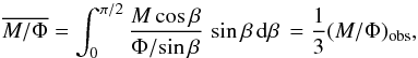 (D.14)where β is the inclination angle with respect to the line of sight, and the sinβ dependence in the flux comes from B = B⊥sinβ, (Crutcher et al. 2004). For a sphere there is no cosβ dependence and fdp = 1 / 2. For a prolate spheroid elongated along the orientation of the field, the mass is multiplied by sinβ instead of cosβ, resulting in fdp = 3 / 4. Investigating which geometry, if any, is most relevant to the actual MCs and the magnetized structures detected within them is obviously important before firm conclusions can be drawn regarding gravitational instability.
Appendix D.5: Discussion
Our estimates of the magnetic field strengths in the MCs analysed and the mass-to-flux ratios, presented in Table D.1, stem from the classic calculation presented by Chandrasekhar & Fermi (1953) and an updated interpretation presented by Hildebrand et al. (2009). Both of these methods assume very specific conditions, so (as we discuss below) this limits the conclusions that can be drawn from these estimates of the magnetic field strength. The deduced mass-to-flux ratios suggest that the clouds are potentially magnetically sub-critical, but we again need to be cautious about drawing conclusions from this application of the DCF and DCF+SF analyses alone.
In the case of the DCF method, the values of are obtained by assuming that the structure of the magnetic field is the product only of incompressible Alfvén waves, where the displacements are perpendicular to the direction of propagation. This is not the case for turbulence in MCs where the random component of the magnetic field can have any orientation. The dispersion measured about mean fields, assumed to be straight in DCF, may be much larger than should be attributed to MHD waves or turbulence, leading to an overestimation of ςψ and to low values of B⊥. Moreover true interstellar turbulence in MCs involves not only incompressible Alfvén waves, but also compressible magneto-sonic waves, which do not satisfy Eq. (D.1). Furthermore, depending on the scales examined, the magnetic field may have structures due to effects such as differential rotation, gravitational collapse, or expanding Hii regions.
In the case of the DCF+SF method, the values of are obtained by assuming a very specific model of the magnetic field, which is in principle just a first-order approximation. First, this model assumes that the effect of the large-scale structured magnetic field, B0, is to cause the square of the second-order structure function, , to increase as ℓ2. This corresponds to a very specific correlation function for B0. Second, this model assumes that the dispersion of the random component of the field, Br, is scale-independent, which is not realistic for the range of scales probed by Planck (Elmegreen & Scalo 2004; Hennebelle & Falgarone 2012).
In addition, the magnetic field orientation deduced from the polarization angle in a particular direction is not generally that of the field at a single point along the line of sight. The observed polarization is the average of various field pseudo-vectors weighted by local dust emission along the line of sight. The net effect of the integration of multiple uncorrelated components along the line of sight is an observed dispersion of the polarization angle that is smaller than the true 3D dispersion of the magnetic field orientation, thus leading to an overestimation of B⊥. Myers & Goodman (1991) presented an analysis of this effect in terms of the number of correlation lengths of the magnetic field along the line of sight through a cloud, which they calculated empirically.
Houde et al. (2009) presented an extension of the DCF+SF method that includes the effect of signal integration along the line of sight and across the area subtended by the telescope beam. The extended method, also implemented in Houde et al. (2011, 2013), is based on the identification of the magnetized turbulence correlation length (δ) by means of the structure function of the polarization angles. In the case of the Planck 353 GHz observations, the angular resolution is not sufficient to identify δ and the corrections would have to rely on rough estimates of this value and the depth of integration (Δ). Following Eq. (29) in Houde et al. (2009), rough estimates δ ≈ 0.2 pc and Δ ≈ 10 pc result in a few correlation lengths across the beam, corresponding to correction factors around 0.4. Coincidentally, such correction factors lead to values of close to those of in Table D.1. But note that this correction relies on specific assumptions on the nature of the turbulence correlation function, it does not circumvent the necessity to observe the dust polarized emission with higher angular resolution to fully characterize the magnetic field.
MHD simulations provide a potentially useful guide to what modifications might be introduced into the DCF formula to allow for inhomogeneity and line-of-sight averaging. Using synthetic observations of MHD simulations, Ostriker et al. (2001) showed that correcting Eq. (D.1)by a factor  provides a good approximation to the actual magnetic field strength in cases where ςψ< 25°. However, the effect of nonlinear amplitudes is uncertain (Zweibel 1996), and the method fails for values of ςψ> 25°, which is the case for all of the regions in this study (Table D.1). Falceta-Gonçalves et al. (2008) propose a method that is potentially valid for any value of ςψ, based on a fit to the values obtained from maps at different resolutions, again concluding that the field should be lower than estimated with Eq. (D.1). However, this approach was not tested in MHD simulations that include gravity, which is the critical process that we aim to evaluate by using the DCF method.
Another strong assumption is that the behaviour of the velocity and the magnetic field are represented well by the observed quantities σv∥ and ςψ for a particular set of scales, which might not necessarily be the case. Even if the power spectra of v and B are comparable in 3D, the integration along the line of sight is different for the two quantities. The dispersion σv∥ is based on the emission-line profile v∥ tracing a gas species, and while the emission is directly integrated along the line of sight, the line profile is possibly affected by radiative transfer and excitation effects. The tracer of the magnetic field is the optically-thin polarized submillimetre emission of dust, and both the polarization and B⊥ are projected and integrated along the line of sight as pseudo-vectors.
Finally, in the estimates of and , a common mean density ρ has been adopted, while in practice ρ is different from cloud to cloud. Direct estimation of the values of ρ from the measured column densities ⟨NH⟩ and ⟨NH2⟩ relies heavily on the geometrical modelling of the cloud and the filling factors of each species, introducing uncertainties that affect the calculated values of B⊥.
Given the line-of-sight integration and the fact that ςψ> 25° uniformly, the calculated values could be considered as upper limits to the actual B⊥. However, other shortcomings, such as the assumptions about the correlation structure and the uncertainties in the determination of the density, do not necessarily bias the estimate of the magnetic field strength towards high values. In conclusion, the values presented in Table D.1 should be viewed only as a reference and only applied with caution, given the many assumptions in both methods at the scales considered.
We use ςψ to avoid confusion with σψ, which was introduced in Planck Collaboration Int. XIX (2015) as the uncertainty in the polarization angle ψ.
Planck (http://www.esa.int/Planck) is a project of the European Space Agency (ESA) with instruments provided by two scientific consortia funded by ESA member states (in particular the lead countries France and Italy), with contributions from NASA (USA) and telescope reflectors provided by a collaboration between ESA and a scientific consortium led and funded by Denmark.
In equatorial coordinates.
In this paper we use the version of arctan with two signed arguments to resolve the π ambiguity in the orientation of pseudo-vectors (Planck Collaboration Int. XIX 2015).
Acknowledgments
The development of Planck has been supported by: ESA; CNES and CNRS/INSU-IN2P3-INP (France); ASI, CNR, and INAF (Italy); NASA and DoE (USA); STFC and UKSA (UK); CSIC, MICINN, JA, and RES (Spain); Tekes, AoF, and CSC (Finland); DLR and MPG (Germany); CSA (Canada); DTU Space (Denmark); SER/SSO (Switzerland); RCN (Norway); SFI (Ireland); FCT/MCTES (Portugal); and PRACE (EU). A description of the Planck Collaboration and a list of its members, including the technical or scientific activities in which they have been involved, can be found at http://www.sciops.esa.int/index.php?project=planck&page=Planck_Collaboration. The research leading to these results has received funding from the European Research Council under the European Union’s Seventh Framework Programme (FP7/2007-2013)/ERC grant agreement No. 267934.
References
- Andersson, B.-G. 2015, in Astrophys. Space Sci. Libr. 407, eds. A. Lazarian, E. M. de Gouveia Dal Pino, & C. Melioli, 59 [Google Scholar]
- Arzoumanian, D., André, P., Peretto, N., & Könyves, V. 2013, A&A, 553, A119 [NASA ADS] [CrossRef] [EDP Sciences] [Google Scholar]
- Audit, E., & Hennebelle, P. 2005, A&A, 433, 1 [NASA ADS] [CrossRef] [EDP Sciences] [Google Scholar]
- Ballesteros-Paredes, J., Hartmann, L., & Vázquez-Semadeni, E. 1999, ApJ, 527, 285 [NASA ADS] [CrossRef] [Google Scholar]
- Bally, J. 2008, Overview of the Orion Complex, ed. B. Reipurth, 4, 459 [Google Scholar]
- Bally, J., Walawender, J., Johnstone, D., Kirk, H., & Goodman, A. 2008, The Perseus Cloud, ed. B. Reipurth, 308 [Google Scholar]
- Banerjee, R., Vázquez-Semadeni, E., Hennebelle, P., & Klessen, R. S. 2009, MNRAS, 398, 1082 [NASA ADS] [CrossRef] [Google Scholar]
- Benoît, A., Ade, P., Amblard, A., et al. 2004, A&A, 424, 571 [NASA ADS] [CrossRef] [EDP Sciences] [Google Scholar]
- Bergin, E. A., & Tafalla, M. 2007, ARA&A, 45, 339 [NASA ADS] [CrossRef] [Google Scholar]
- Bierman, E. M., Matsumura, T., Dowell, C. D., et al. 2011, ApJ, 741, 81 [NASA ADS] [CrossRef] [Google Scholar]
- Burkhart, B., Lazarian, A., Leão, I. C., de Medeiros, J. R., & Esquivel, A. 2014, ApJ, 790, 130 [NASA ADS] [CrossRef] [Google Scholar]
- Cabral, B., & Leedom, L. C. 1993, in Special Interest Group on GRAPHics and Interactive Techniques Proceedings, 263 [Google Scholar]
- Chandrasekhar, S., & Fermi, E. 1953, ApJ, 118, 113 [NASA ADS] [CrossRef] [Google Scholar]
- Chapman, N. L., Goldsmith, P. F., Pineda, J. L., et al. 2011, ApJ, 741, 21 [NASA ADS] [CrossRef] [Google Scholar]
- Comerón, F. 2008, The Lupus Clouds, ed. B. Reipurth, 5, 295 [Google Scholar]
- Crutcher, R. M. 2005, in Magnetic Fields in the Universe: From Laboratory and Stars to Primordial Structures, eds. E. M. de Gouveia dal Pino, G. Lugones, & A. Lazarian, AIP Conf. Ser., 784, 129 [Google Scholar]
- Crutcher, R. M. 2012, ARA&A, 50, 29 [NASA ADS] [CrossRef] [Google Scholar]
- Crutcher, R. M., Nutter, D. J., Ward-Thompson, D., & Kirk, J. M. 2004, ApJ, 600, 279 [NASA ADS] [CrossRef] [Google Scholar]
- Crutcher, R. M., Wandelt, B., Heiles, C., Falgarone, E., & Troland, T. H. 2010, ApJ, 725, 466 [NASA ADS] [CrossRef] [Google Scholar]
- Dame, T. M., Hartmann, D., & Thaddeus, P. 2001, ApJ, 547, 792 [NASA ADS] [CrossRef] [Google Scholar]
- Davis, L. 1951, Phys. Rev., 81, 890 [NASA ADS] [CrossRef] [PubMed] [Google Scholar]
- Davis, Jr., L., & Greenstein, J. L. 1951, ApJ, 114, 206 [Google Scholar]
- Dotson, J. L. 1996, ApJ, 470, 566 [NASA ADS] [CrossRef] [Google Scholar]
- Dotson, J. L., Davidson, J., Dowell, C. D., Schleuning, D. A., & Hildebrand, R. H. 2000, ApJS, 128, 335 [NASA ADS] [CrossRef] [Google Scholar]
- Draine, B. T. 2011, Physics of the Interstellar and Intergalactic Medium (Princeton University Press) [Google Scholar]
- Eiroa, C., Djupvik, A. A., & Casali, M. M. 2008, The Serpens Molecular Cloud, ed. B. Reipurth, 693 [Google Scholar]
- Elmegreen, B. G., & Scalo, J. 2004, ARA&A, 42, 211 [NASA ADS] [CrossRef] [Google Scholar]
- Falceta-Gonçalves, D., Lazarian, A., & Kowal, G. 2008, ApJ, 679, 537 [NASA ADS] [CrossRef] [Google Scholar]
- Franco, G. A. P., Alves, F. O., & Girart, J. M. 2010, ApJ, 723, 146 [Google Scholar]
- Goldreich, P., & Sridhar, S. 1995, ApJ, 438, 763 [NASA ADS] [CrossRef] [Google Scholar]
- Górski, K. M., Hivon, E., Banday, A. J., et al. 2005, ApJ, 622, 759 [NASA ADS] [CrossRef] [Google Scholar]
- Hartmann, L., Ballesteros-Paredes, J., & Bergin, E. A. 2001, ApJ, 562, 852 [NASA ADS] [CrossRef] [Google Scholar]
- Harvey, P. M., Huard, T. L., Jørgensen, J. K., et al. 2008, ApJ, 680, 495 [NASA ADS] [CrossRef] [Google Scholar]
- Heiles, C., & Haverkorn, M. 2012, Space Sci. Rev., 166, 293 [NASA ADS] [CrossRef] [EDP Sciences] [Google Scholar]
- Heitsch, F., Zweibel, E. G., Mac Low, M.-M., Li, P., & Norman, M. L. 2001, ApJ, 561, 800 [NASA ADS] [CrossRef] [Google Scholar]
- Heitsch, F., Slyz, A. D., Devriendt, J. E. G., Hartmann, L. W., & Burkert, A. 2006, ApJ, 648, 1052 [NASA ADS] [CrossRef] [Google Scholar]
- Heitsch, F., Stone, J. M., & Hartmann, L. W. 2009, ApJ, 695, 248 [NASA ADS] [CrossRef] [Google Scholar]
- Hennebelle, P. 2013, A&A, 556, A153 [NASA ADS] [CrossRef] [EDP Sciences] [Google Scholar]
- Hennebelle, P., & Falgarone, E. 2012, A&ARv, 20, 55 [NASA ADS] [CrossRef] [Google Scholar]
- Heyer, M., Gong, H., Ostriker, E., & Brunt, C. 2008, ApJ, 680, 420 [NASA ADS] [CrossRef] [Google Scholar]
- Hildebrand, R. H. 1988, QJRAS, 29, 327 [NASA ADS] [Google Scholar]
- Hildebrand, R. H., Kirby, L., Dotson, J. L., Houde, M., & Vaillancourt, J. E. 2009, ApJ, 696, 567 [NASA ADS] [CrossRef] [Google Scholar]
- Hiltner, W. A. 1949, Science, 109, 165 [NASA ADS] [CrossRef] [Google Scholar]
- Hoang, T., & Lazarian, A. 2009, ApJ, 697, 1316 [Google Scholar]
- Houde, M., Vaillancourt, J. E., Hildebrand, R. H., Chitsazzadeh, S., & Kirby, L. 2009, ApJ, 706, 1504 [NASA ADS] [CrossRef] [Google Scholar]
- Houde, M., Rao, R., Vaillancourt, J. E., & Hildebrand, R. H. 2011, ApJ, 733, 109 [NASA ADS] [CrossRef] [Google Scholar]
- Houde, M., Fletcher, A., Beck, R., et al. 2013, ApJ, 766, 49 [NASA ADS] [CrossRef] [Google Scholar]
- Inoue, T., & Inutsuka, S.-i. 2009, ApJ, 704, 161 [NASA ADS] [CrossRef] [Google Scholar]
- Jones, T. J., Bagley, M., Krejny, M., Andersson, B.-G., & Bastien, P. 2015, AJ, 149, 31 [NASA ADS] [CrossRef] [Google Scholar]
- Kenyon, S. J., Gómez, M., & Whitney, B. A. 2008, Low Mass Star Formation in the Taurus-Auriga Clouds, ed. B. Reipurth, 4, 405 [Google Scholar]
- Knude, J., & Hog, E. 1998, A&A, 338, 897 [NASA ADS] [Google Scholar]
- Kobulnicky, H. A., Molnar, L. A., & Jones, T. J. 1994, AJ, 107, 1433 [NASA ADS] [CrossRef] [Google Scholar]
- Koch, P. M., Tang, Y.-W., & Ho, P. T. P. 2013, ApJ, 775, 77 [NASA ADS] [CrossRef] [Google Scholar]
- Koyama, H., & Inutsuka, S.-i. 2002, ApJ, 564, L97 [NASA ADS] [CrossRef] [Google Scholar]
- Kun, M., Kiss, Z. T., & Balog, Z. 2008, Star Forming Regions in Cepheus, ed. B. Reipurth, 136 [Google Scholar]
- Lamarre, J., Puget, J., Ade, P. A. R., et al. 2010, A&A, 520, A9 [NASA ADS] [CrossRef] [EDP Sciences] [Google Scholar]
- Lazarian, A., & Hoang, T. 2007, MNRAS, 378, 910 [Google Scholar]
- Lazarian, A., & Vishniac, E. T. 1999, ApJ, 517, 700 [NASA ADS] [CrossRef] [Google Scholar]
- Li, H.-B., & Houde, M. 2008, ApJ, 677, 1151 [NASA ADS] [CrossRef] [Google Scholar]
- Li, H., Griffin, G. S., Krejny, M., et al. 2006, ApJ, 648, 340 [NASA ADS] [CrossRef] [Google Scholar]
- Li, H.-B., Fang, M., Henning, T., & Kainulainen, J. 2013, MNRAS, 436, 3707 [NASA ADS] [CrossRef] [Google Scholar]
- Luhman, K. L. 2008, Chamaeleon, ed. B. Reipurth, 5, 169 [Google Scholar]
- Martin, P. G., Roy, A., Bontemps, S., et al. 2012, ApJ, 751, 28 [NASA ADS] [CrossRef] [Google Scholar]
- Matthaeus, W. H., Pouquet, A., Mininni, P. D., Dmitruk, P., & Breech, B. 2008, Phys. Rev. Lett., 100, 085003 [NASA ADS] [CrossRef] [Google Scholar]
- Matthews, B. C., Wilson, C. D., & Fiege, J. D. 2001, ApJ, 562, 400 [NASA ADS] [CrossRef] [Google Scholar]
- Matthews, B. C., McPhee, C. A., Fissel, L. M., & Curran, R. L. 2009, ApJS, 182, 143 [NASA ADS] [CrossRef] [Google Scholar]
- Matthews, T. G., Ade, P. A. R., Angilè, F. E., et al. 2014, ApJ, 784, 116 [NASA ADS] [CrossRef] [Google Scholar]
- McKee, C. F., & Ostriker, E. C. 2007, ARA&A, 45, 565 [NASA ADS] [CrossRef] [Google Scholar]
- McKee, C. F., Zweibel, E. G., Goodman, A. A., & Heiles, C. 1993, in Protostars and Planets III, eds. E. H. Levy, & J. I. Lunine, 327 [Google Scholar]
- Molinari, S., Schisano, E., Faustini, F., et al. 2011, A&A, 530, A133 [NASA ADS] [CrossRef] [EDP Sciences] [Google Scholar]
- Moneti, A., Pipher, J. L., Helfer, H. L., McMillan, R. S., & Perry, M. L. 1984, ApJ, 282, 508 [NASA ADS] [CrossRef] [Google Scholar]
- Montier, L., Plaszczynski, S., Levrier, F., et al. 2015, A&A, 574, A135 [NASA ADS] [CrossRef] [EDP Sciences] [Google Scholar]
- Mouschovias, T. C. 1976a, ApJ, 206, 753 [NASA ADS] [CrossRef] [Google Scholar]
- Mouschovias, T. C. 1976b, ApJ, 207, 141 [NASA ADS] [CrossRef] [Google Scholar]
- Mouschovias, T. C. 1991, ApJ, 373, 169 [NASA ADS] [CrossRef] [Google Scholar]
- Myers, P. C., & Goodman, A. A. 1991, ApJ, 373, 509 [NASA ADS] [CrossRef] [Google Scholar]
- Nakano, T. 1998, ApJ, 494, 587 [NASA ADS] [CrossRef] [Google Scholar]
- Nakano, T., & Nakamura, T. 1978, PASJ, 30, 671 [NASA ADS] [Google Scholar]
- Neuhäuser, R., & Forbrich, J. 2008, The Corona Australis Star Forming Region, ed. B. Reipurth, 735 [Google Scholar]
- Ostriker, E. C., Stone, J. M., & Gammie, C. F. 2001, ApJ, 546, 980 [NASA ADS] [CrossRef] [Google Scholar]
- Palmeirim, P., André, P., Kirk, J., et al. 2013, A&A, 550, A38 [NASA ADS] [CrossRef] [EDP Sciences] [Google Scholar]
- Paradis, D., Dobashi, K., Shimoikura, T., et al. 2012, A&A, 543, A103 [NASA ADS] [CrossRef] [EDP Sciences] [Google Scholar]
- Pereyra, A., & Magalhães, A. M. 2004, ApJ, 603, 584 [NASA ADS] [CrossRef] [Google Scholar]
- Planck Collaboration XXIV. 2011, A&A, 536, A24 [Google Scholar]
- Planck Collaboration I. 2014, A&A, 571, A1 [NASA ADS] [CrossRef] [EDP Sciences] [Google Scholar]
- Planck Collaboration II. 2014, A&A, 571, A2 [NASA ADS] [CrossRef] [EDP Sciences] [Google Scholar]
- Planck Collaboration V. 2014, A&A, 571, A5 [NASA ADS] [CrossRef] [EDP Sciences] [Google Scholar]
- Planck Collaboration VI. 2014, A&A, 571, A6 [NASA ADS] [CrossRef] [EDP Sciences] [Google Scholar]
- Planck Collaboration VIII. 2014, A&A, 571, A8 [NASA ADS] [CrossRef] [EDP Sciences] [Google Scholar]
- Planck Collaboration XI. 2014, A&A, 571, A11 [NASA ADS] [CrossRef] [EDP Sciences] [Google Scholar]
- Planck Collaboration Int. XIX. 2015, A&A, 576, A104 [NASA ADS] [CrossRef] [EDP Sciences] [Google Scholar]
- Planck Collaboration Int. XX. 2015, A&A, 576, A105 [NASA ADS] [CrossRef] [EDP Sciences] [Google Scholar]
- Planck Collaboration Int. XXI. 2015, A&A, 576, A106 [NASA ADS] [CrossRef] [EDP Sciences] [Google Scholar]
- Planck Collaboration Int. XXXII. 2016, A&A, 586, A135 [NASA ADS] [CrossRef] [EDP Sciences] [Google Scholar]
- Planck Collaboration Int. XXXIII. 2016, A&A, 586, A136 [NASA ADS] [CrossRef] [EDP Sciences] [Google Scholar]
- Poppel, W. 1997, Fund. Cosmic Phys., 18, 1 [Google Scholar]
- Prato, L., Rice, E. L., & Dame, T. M. 2008, Where are all the Young Stars in Aquila?, ed. B. Reipurth, 4, 18 [Google Scholar]
- Reipurth, B. 2008, Handbook of Star Forming Regions, Volume I: The Northern Sky, 4 [Google Scholar]
- Santos, F. P., Franco, G. A. P., Roman-Lopes, A., Reis, W., & Román-Zúñiga, C. G. 2014, ApJ, 783, 1 [NASA ADS] [CrossRef] [Google Scholar]
- Santos-Lima, R., de Gouveia Dal Pino, E. M., & Lazarian, A. 2012, ApJ, 747, 21 [NASA ADS] [CrossRef] [Google Scholar]
- Schlafly, E. F., Green, G., Finkbeiner, D. P., et al. 2014, ApJ, 786, 29 [NASA ADS] [CrossRef] [Google Scholar]
- Serkowski, K. 1958, Acta Astron., 8, 135 [NASA ADS] [Google Scholar]
- Soler, J. D., Hennebelle, P., Martin, P. G., et al. 2013, ApJ, 774, 128 [NASA ADS] [CrossRef] [Google Scholar]
- Spitzer, Jr., L. 1968, Interscience Tracts on Physics and Astronomy, 28, 262 [Google Scholar]
- Sridhar, S., & Goldreich, P. 1994, ApJ, 432, 612 [NASA ADS] [CrossRef] [Google Scholar]
- Straižys, V., Černis, K., & Bartašiūtė, S. 2003, A&A, 405, 585 [NASA ADS] [CrossRef] [EDP Sciences] [Google Scholar]
- Sugitani, K., Nakamura, F., Watanabe, M., et al. 2011, ApJ, 734, 63 [Google Scholar]
- Tassis, K., Dowell, C. D., Hildebrand, R. H., Kirby, L., & Vaillancourt, J. E. 2009, MNRAS, 399, 1681 [NASA ADS] [CrossRef] [Google Scholar]
- Ward-Thompson, D., Kirk, J. M., Crutcher, R. M., et al. 2000, ApJ, 537, L135 [NASA ADS] [CrossRef] [Google Scholar]
- Whittet, D. C. B., Prusti, T., Franco, G. A. P., et al. 1997, A&A, 327, 1194 [NASA ADS] [Google Scholar]
- Whittet, D. C. B., Hough, J. H., Lazarian, A., & Hoang, T. 2008, ApJ, 674, 304 [NASA ADS] [CrossRef] [Google Scholar]
- Wilking, B. A., Gagné, M., & Allen, L. E. 2008, Star Formation in the ρ Ophiuchi Molecular Cloud, ed. B. Reipurth, 5, 351 [Google Scholar]
- Zweibel, E. G. 1996, in Polarimetry of the Interstellar Medium, ed. W. G. Roberge, & D. C. B. Whittet, ASP Conf. Ser., 97, 486 [Google Scholar]
All Tables
All Figures
|
Fig. 1 Magnetic field and column density measured by Planck towards the Taurus MC. The colours represent column density. The “drapery” pattern, produced using the line integral convolution method (LIC, Cabral & Leedom 1993), indicates the orientation of magnetic field lines, orthogonal to the orientation of the submillimetre polarization. |
| In the text | |
|
Fig. 2 Locations and sizes of the regions selected for analysis. The background map is the gas column density, NH, derived from the dust optical depth at 353 GHz (Planck Collaboration XI 2014). |
| In the text | |
|
Fig. 3 Left: columm density map, log 10(NH/ cm-2), overlaid with magnetic field pseudo-vectors whose orientations are inferred from the Planck 353 GHz polarization observations. The length of the pseudo-vectors is normalized so does not reflect the polarization fraction. In this first group, the regions analysed are, from top to bottom, Taurus, Ophiuchus, Lupus, Chamaeleon-Musca, and CrA. Right: HROs for the lowest, an intermediate, and the highest NH bin (black, blue, and red, respectively). For a given region, bins have equal numbers of selected pixels (see Sect. 4.1.1 and Appendix A) within the NH ranges labelled. The intermediate bin corresponds to selected pixels near the blue contours in the column density images. The horizontal dashed line corresponds to the average per angle bin of 15°. The widths of the shaded areas for each histogram correspond to the ± 1σ uncertainties related to the histogram binning operation. Histograms peaking at 0° correspond to B⊥ predominantly aligned with iso-NH contours. Histograms peaking at 90° and/or − 90° correspond to B⊥ predominantly perpendicular to iso-NH contours. |
| In the text | |
|
Fig. 3 continued. |
| In the text | |
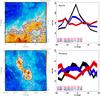 |
Fig. 4 Same as Fig. 3 for the second group, Aquila Rift and Perseus. |
| In the text | |
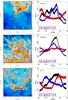 |
Fig. 5 Same as Fig. 3 for the third group, IC 5146, Cepheus, and Orion. |
| In the text | |
|
Fig. 6 Schematic of the vectors involved in the calculation of the relative orientation angle φ. |
| In the text | |
|
Fig. 7 Histogram shape parameter ξ (Eqs. (4) and (5)) calculated for the different NH bins in each region. The cases ξ> 0 and ξ< 0 correspond to the magnetic field oriented mostly parallel and perpendicular to the structure contours, respectively. For ξ ≈ 0 there is no preferred orientation. The displayed values of CHRO and XHRO were calculated from Eq. (6)and correspond to the grey dashed line in each plot. |
| In the text | |
|
Fig. 8 Same as Fig. 3 for the two test regions located directly east (ChamEast) and south of Chamaeleon-Musca (ChamSouth). |
| In the text | |
|
Fig. 9 Maps of the absolute value of the relative orientation angle, | φ |, in the Taurus region. These maps are produced after smoothing the input maps to beam FWHMs of 10′, 15′, 30′, and 60′ and then resampling the grid to sample each beam FWHM with the same number of pixels. The regions in red correspond to B⊥ close to perpendicular to NH structures. The regions in blue correspond to B⊥ close to parallel to NH structures. The black contour, corresponding to the NH value of the intermediate contour introduced in Fig. 3, provides a visual reference to the cloud structure. |
| In the text | |
|
Fig. 10 HROs of the Taurus region after smoothing the input maps to beam FWHMs of 15′, 30′, and 60′, shown from left to right, respectively. |
| In the text | |
|
Fig. 11 Histogram shape parameter ξ (Eqs. (4) and (5)) calculated for the different NH bins in each region. Top: relative orientation in synthetic observations of simulations with super-Alfvénic (blue), Alfvénic (green), and sub-Alfvénic (red) turbulence, as detailed in Soler et al. (2013). Middle: relative orientation in the regions selected from the Planck all-sky observations, from Fig. 7. The blue data points correspond to the lowest NH regions (CrA and the test regions in Fig. 8, ChamSouth and ChamEast) and the orange correspond to the rest of the clouds. Bottom: comparison between the trends in the synthetic observations (in colours) and the regions studied (grey). The observed smooth transition from mostly parallel (ξ> 0) to perpendicular (ξ< 0) is similar to the transition in the simulations for which the turbulence is Alfvénic or sub-Alfvéic. |
| In the text | |
|
Fig. B.1 HROs in the Taurus region that correspond to the indicated NH bins. The plotted values are obtained using the original τ353 map at 10′ resolution and maps of the Stokes parameters Qr and Ur, which correspond to 1000 random noise realizations. Each realization is generated using a Gaussian probability density function centred on the measured values Q and U with variances |
| In the text | |
|
Fig. B.2 Histogram shape parameter, ξ, as a function of log 10(NH/ cm-2) in the Taurus region. The values are obtained using the τ353 map at 10′ resolution and maps of the Stokes parameters Qr and Ur that correspond to 1000 random-noise realizations. Each realization is generated using a Gaussian probability density function centred on the measured values Q and Uwith variances |
| In the text | |
|
Fig. C.1 Histogram shape parameter, ξ, as a function of log 10(NH/ cm-2) in the Taurus region. Blue lines join the ξ values obtained using the τ353 map at 10′ resolution and each of 1000 random realizations of Q and U maps corresponding to a uniform distribution of ψ. Results in black and grey are from the analysis of the Planck data, as reported in Fig. 7. |
| In the text | |
|
Fig. C.2 Like Fig. C.1 but for values of ξ (red) obtained using 1000 random realizations of Q and U maps corresponding to a Gaussian distribution of ψ centred on ψ0 = 0° and with standard deviation ςψ = 45°. |
| In the text | |
|
Fig. C.3 Like Fig. C.1 but for values of ξ (green) obtained using 1000 random realizations of Q and U maps corresponding to a power spectrum P(k) ∝ kαm, with αm = −1.5, − 2.5, and − 3.5. |
| In the text | |
|
Fig. C.4 Histogram shape parameter, ξ, as a function of log 10(NH/ cm-2) calculated from the τ353 map at 10′ resolution in the Taurus region and the Stokes Q and U maps shifted in Galactic longitude and latitude by the values indicated, for Δl and Δb, respectively. |
| In the text | |
|
Fig. C.5 Normalized distributions of relative orientations of random vectors in 3D (top) and of their projections in 2D (bottom). The curves correspond to mostly perpendicular vectors (red), uniform distribution of relative orientations (black), and mostly parallel vectors (green). The solid, dashed, and dotted lines correspond to dispersions of the relative orientation angle ςα = 18°, 36°, and 72°, respectively. |
| In the text | |
|
Fig. D.1 Line-of-sight centroid velocity v∥ maps inferred from CO emission (Dame et al. 2001). Areas shown have sufficient S/N in the polarization observations (second polarization criterion in Appendix A.2) for the DCF and DCF+SF analyses and lie in the range − 10 <v∥/ (km s-1) < 10. |
| In the text | |
|
Fig. D.2 Structure function S2(ℓ) calculated from the Q and U maps of the selected regions following Eq. (D.4). The black lines indicate the fits given by Eq. (D.6). The vertical dashed line marks the common 10′ resolution of the data used in the analysis; the data are correlated for low values of ℓ causing the drop in S2(ℓ). |
| In the text | |
Current usage metrics show cumulative count of Article Views (full-text article views including HTML views, PDF and ePub downloads, according to the available data) and Abstracts Views on Vision4Press platform.
Data correspond to usage on the plateform after 2015. The current usage metrics is available 48-96 hours after online publication and is updated daily on week days.
Initial download of the metrics may take a while.