| Issue |
A&A
Volume 575, March 2015
|
|
|---|---|---|
| Article Number | A41 | |
| Number of page(s) | 17 | |
| Section | Astronomical instrumentation | |
| DOI | https://doi.org/10.1051/0004-6361/201424897 | |
| Published online | 18 February 2015 | |
Evidence for self-interaction of charge distribution in charge-coupled devices
1
LPNHE, CNRS-IN2P3 and Universités Paris 6 & 7,
4 place Jussieu,
75252
Paris Cedex 05,
France
e-mail:
guyonnet@lpnhe.in2p3.fr
2
Department of Physics, Harvard University,
17 Oxford Street, Cambridge, MA
02138,
USA
Received: 1 September 2014
Accepted: 19 December 2014
Charge-coupled devices (CCDs) are widely used in astronomy to carry out a variety of measurements, such as for flux or shape of astrophysical objects. The data reduction procedures almost always assume that the response of a given pixel to illumination is independent of the content of the neighboring pixels. We show evidence that this simple picture is not exact for several CCD sensors. Namely, we provide evidence that localized distributions of charges (resulting from star illumination or laboratory luminous spots) tend to broaden linearly with increasing brightness by up to a few percent over the whole dynamic range. We propose a physical explanation for this “brighter-fatter” effect, which implies that flatfields do not exactly follow Poisson statistics: the variance of flatfields grows less rapidly than their average, and neighboring pixels show covariances, which increase similarly to the square of the flatfield average. These covariances decay rapidly with pixel separation. We observe the expected departure from Poisson statistics of flatfields on CCD devices and show that the observed effects are compatible with Coulomb forces induced by stored charges that deflect forthcoming charges. We extract the strength of the deflections from the correlations of flatfield images and derive the evolution of star shapes with increasing flux. We show for three types of sensors that within statistical uncertainties, our proposed method properly bridges statistical properties of flatfields and the brighter-fatter effect.
Key words: instrumentation: detectors / methods: data analysis / techniques: photometric / astronomical databases: miscellaneous / telescopes / techniques: image processing
© ESO, 2015
1. Introduction
Charge-coupled devices (CCDs) for astronomy are often pictured as a regular lattice of “charge receivers”, which transform incoming light into independent pixels in an almost linear fashion. Reduction techniques generally assume that the response of each pixel is independent of the charge content of its neighbors. This representation even accommodates the non-linearity of a pixel response, typically attributed to the electronic chain. Once linearity is restored, the data reduction usually relies on the hypothesis that the response to a source of light of a given shape just scales with its flux. For devices observing the sky, the overall response of an imaging system is described by its point spread function (PSF), which is, in practice, the response to stars, because they are not resolved. Astronomical softwares (e.g., DaoPhot, PSFeX) commonly assume that star images are homothetic and hence that bright stars can be used to account for the impact of the whole instrument (possibly including atmosphere) on the observed shapes of other objects, which are typically faint stars or galaxies. For example, bright stars are also commonly used to model the shape of faint stars, which allows one to measure optimally the flux and position of the latter with respect to shot noise.
Do star images really scale with their flux? Lateral diffusion of charges during their drift in the silicon does not break this scaling, except for an effect that we discuss later. Obviously, at some point, the scaling breaks down because some sort of saturation occurs in either the sensors themselves (charge buckets overflow), or the electronic chain (some signals saturate). However, well below saturation, the scaling of stars images is assumed to be exact. We show in this paper that this is not usually true at all brightness levels and that the effect cannot be ignored for some scientific applications.
There is a well-known hint that CCD pixels are sensitive to their environment: the variance of flatfields does not rise linearly with illumination, but the rise flattens out, departing from exact Poisson statistics (Downing et al. 2006). This effect tends to vanish when one rebins the image prior to computing the statistics, indicating that the variance of a sum of neighboring pixels is larger than the sum of their variances. Neighbor pixels should therefore be positively correlated (as found in Downing et al. 2006), and in this paper we present direct measurements that confirm this.
If some physical phenomenon tends to reduce the variance of flatfields, one might expect the same phenomenon to also smooth stellar images. We show that a variety of CCD sensors deliver stellar images that broaden with increasing flux at least to some level. This “brighter-fatter” effect complicates the direct use of stars as PSF models.
There are currently large-scale imaging programs, either underway or planned, that intend to measure the cosmic gravitational shear induced by mass concentrations that are located between background galaxies and observers by evaluating the average elongation of galaxy images (e.g., Chang et al. 2013). These programs vitally rely on the shape of stars in the science images, which are used to measure and account for the distortions induced by the observing system on the background galaxies. It is mandatory for these programs that the characteristics of the PSF and, in particular, its angular size are accurately measured, typically to a fractional accuracy of ~10-3 (Bernstein & Jarvis 2002; Amara & Réfrégier 2008). For the Euclid space mission, it is required that the PSF ellipticity is known to 0.02%, and the PSF size to 0.1% (Laureijs et al. 2011). Since the scaling of stellar images is for some sensors violated at a few percent level, bright stars cannot readily be used as models for the shape distortion induced by the observing system (Melchior et al. 2014).
The evolution of star shapes with flux also adversely impacts the accuracy of PSF photometry of faint sources. Supernova photometry for cosmology has become a demanding application because photometric biases at the ~0.006 mag level seriously impact the precision of cosmological constraints (e.g., Betoule et al. 2014 and references therein). Since supernova photometry consists of measuring the PSF flux ratio of the faint supernovae to that of bright stars around it, ignoring the brighter-fatter effect leads to a relative flux bias equal to the PSF size variation between these two classes of objects (e.g., Astier et al. 2013). Understanding the causes of the brighter-fatter effect is needed to accurately use the stars to model the actual PSF.
In this paper, we show that the correlations between neighbor pixels and the brighter-fatter effect can be explained by alterations to the drift field caused by charges already collected in the potential wells of the CCD. However, the size of the induced distortions and how they decay with distance from the sources both depend on manufacturing details of the CCD. The CCD vendors do not necessarily know these details with a precision sufficient to model the field distortions, or even regard them as proprietary. In this context, relating the statistical correlations between nearby pixels in flatfields and the brighter-fatter effect might be the practical way to derive the details of the latter from measurements of the former. This paper aims to provide encouraging indications that this program is indeed plausible. A previous communication (Antilogus et al. 2014) presented this idea together with preliminary results. Here, we present a refined analysis and describe the matter in more detail.
We use data sets from three different instruments. The first is the MegaCam camera, which has been mounted on the Canada-France-Hawaii Telescope (CFHT), since 2003. The camera is a mosaic of 36 thinned CCDs. The two other instruments are both equipped with deep-depletion sensors. One is the DECam camera that has been mounted on the Blanco four-meter telescope at CTIO since 2012. DECam is a mosaic of 62 CCDs. The other is a CCD from E2V that is being tested by the LSST collaboration as a candidate for the focal plane of the future LSST telescope (Sect. 2). For these instruments, we first establish the existence of both the brighter-fatter effect (Sect. 3) and confirm that correlations in flatfield exposures do exist (Sect. 4). Secondly, we show how taking simple electrostatic repulsion between collected charges and drifting electrons within the CCD bulk into account qualitatively describe both effects (Sect. 5) and that a simple model fitted to correlations in flatfield exposures quantitatively predicts the amplitude of the brighter-fatter effect (Sect. 6), thus giving a practical method to account for the variation of image quality (IQ) versus flux.
2. The sensors and data
The present evolution in camera design, moving from using thinned CCDs to using thick CCDs, corresponds to an improvement of silicon wafer resistivity allowing for depletion of the mobile charge carriers over several hundred microns, which increases detector spatial resolution. This work has gathered data from both types of CCDs to strengthen the evidence that evolution of electrostatic forces within pixels has detectable consequences and that it is a general feature of CCDs.
This section describes the instruments that have been used to establish this hypothesis. For each instrument, the data set is constituted by both point source illumination exposures (using artificial spots or real stars) and by uniform illuminations (called hereafter flatfield illumination exposures, or simply flatfields).
2.1. The MegaCam instrument
Since 2003 MegaCam is a 1 deg2 wide field imager hosted in the dedicated prime focus environment, MegaPrime, on the Canada-France-Hawaii 3.6-m telescope (Boulade et al. 2003). The camera images a field of view of 0.96 × 0.94 deg2 using 36 thinned E2V 42-90 2048 × 4612 CCDs with 13.5μm pixels. Pixels have a conventional three-phase structure with one electrode that defines the collection area and the other two that constitute barriers in transfer direction. Each CCD is read out by two amplifiers, which allows one to read out the whole focal plane in about 35 s. The output of each amplifier is sampled by a 16 bit ADC. The gains of the readout chains have been set to ~1.5 e−/ ADU with the consequence that only half of the CCD full well (~200 000 e−) is actually sampled by the readout electronics. The PSF broadening seen by the MegaCam instrument has been measured using all the CFHT-DEEP r-band exposures obtained during the five years of the CFHT-LS (SNLS) survey. The flatfields that we used are constituted by images that were acquired using the internal illumination capability of the instrument (red LEDs). This setup has been preferred from twilight flatfield because of its better reproductibity when acquiring pair images.
2.2. The DECam instrument
The DECam is a 2.2 deg2 wide field imager (Estrada et al. 2010). It is mounted on the Blanco four-meter telescope at CTIO and is used by the Dark Energy Survey (DES) that has begun on August 31, 2013. It is made of 62 LBL/DALSA 250μm thick, back-illuminated sensors (Holland et al 2003). Each CCD is made of 2048 × 4096 p-channel pixels, which have a width of 15 × 15μm and a thickness of 250μm, with a three-phase structure with full well at ~200 000 e−. Charges collected in the depletion region are stored in the buried channels that are established a few μm away from gate electrodes. Substrate bias is 40 V so as to fully deplete the device, thus reducing charge diffusion to a minimum (measurements indicate ≈6μm at 40 V). Each CCD is read out by two amplifiers.
The data set used in this study comes from publicly available science verification images acquired during the commissioning of the instrument between Summer 2012 and Spring 2013 (Bernstein et al. 2013). Astronomical images are observations in all bands (u, g, r, i, z, Y) of three dense stellar fields at low galactic latitude. For the uniform illuminations, the analysis necessitates high stability of the field: we use flatfields acquired using a screen installed under the dome and illuminated by LEDs (Marshall et al. 2013).
2.3. The LSST CCD E2V-250
The Large Synoptic Survey Telescope (LSST) will carry out a deep astronomical imaging survey of the southern sky. It will use an 8.4-m ground-based telescope with which the construction has begun. The survey is planned to start in 2022 and the LSST collaboration shall soon begin the construction of the focal plane, which will eventually be a 9.6 deg2 wide field imager made of 189 CCDs. The project is currently evaluating candidate sensors from multiple vendors. One of the sensor candidates is a CCD E2V-250, a 4096 × 4096 pixel array that is 100μm thick and equipped with sixteen amplifiers. Each pixel is 10μm on a side and has a four-phase structure so as to reach a full-well capacity of ~160 000 e−.
In this study, we utilize exposures from the CCD E2V-250 that were obtained by the LSST sensor team during December 2012. The test bench setup uses lamps whose output illumination feeds a monochromator. The monochromator output is then either diffused by an integrating sphere to produce a flatfield, or collimated using a pinhole to produce a spot (hereafter called “spot image”).
3. Broadening of spots and stars with increasing fluxes: the brighter-fatter effect
This section presents the amplitude of the broadening of spot or star images that affects both deep-depleted CCDs and thinned devices.
3.1. The broadening of spots with increasing fluxes
The broadening of localized charge distribution when flux increases can be shown directly from a series of artificial spot exposures. In Fig. 1, we propose direct evidence for the broadening of spots with flux on the CCD E2V-250. We subtract an average of 20 s exposure (faint) laboratory spots from an average of 200 s (bright) spot after scaling the flux to take the difference between exposure times into account. The stronger wings and weaker core of the 200 s spot are clearly visible in the result of the subtraction (Fig. 1, right).
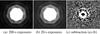 |
Fig. 1 Direct shape comparison of bright and faint spots from the CCD E2V-250. The leftmost image is the average of 200 s exposures; and the middle one averages 20 s exposures; the rightmost image is the difference after proper scaling of 200 s spot image minus 20 s spot images. The broader wings and lower peak of the bright spot clearly show up. Since the images required a small alignment prior to subtraction, we have shifted both averages by half their separation, so that resampling affects both in the same way. |
3.2. Measurement of the apparent size of stars
To perform a quantitative study of the effect, an estimator of size is needed. The apparent size of stars or spots is estimated using elliptical Gaussian weights, whose size are matched to the object (see Astier et al. 2013, Sect. 3). The method is similar, if not identical, to the one proposed in Bernstein & Jarvis (2002). Our method turns out to be equivalent to fitting an elliptical Gaussian to the image with uniform weights. We have checked on simulations of non-Gaussian spots of identical shapes with varying signal-to-noise ratios (S/Ns), which shows this second moment estimator is independent on average of S/N. The combination of the second moments Mxx,Myy,Mxy of the 2D Gaussian distribution defines the image quality (IQ): ![\begin{eqnarray*} IQ = \sqrt[4]{M_{xx} M_{yy}-M_{xy}^2} \end{eqnarray*}](/articles/aa/full_html/2015/03/aa24897-14/aa24897-14-eq20.png) which we use to estimate the apparent size of stars. It should be noted that | Mxy | ≪ Mxx, Myy and that we also refer to the Gaussian root mean square (rms)
which we use to estimate the apparent size of stars. It should be noted that | Mxy | ≪ Mxx, Myy and that we also refer to the Gaussian root mean square (rms)  or
or  as the width of a star or a spot for all data sets considered here.
In astronomical exposures, a small correlation between flux and size through color is expected. On a given field, fluxes are usually correlated with color, meanwhile blue stars tend to be broader than red stars (because image quality tend to improves in redder wavelengths). This dependency is taken into account by fitting size versus color relation using low flux stars. The correction is small on MegaCam data and negligible on DECam.
3.3. Results
Broadening of spots and stars that is seen on all the images and taken with the three instruments are summarized on the panels of Fig. 2. The amplitude of the effect is normalized by the reference sizes of the spots/stars as a mean to compare its impact on the various data samples relative to their IQ. For each instrument, the intervals that are presented have been selected for a dynamic range that is below blooming effects, a degradation of the charge transfer efficiency of CCDs that occurs at a level close to full well, but that varies with CCD readout parameters (see Sect. 4). This directly affects the spot size measurement, with a threshold that is around 130 ke− and 170 ke−, respectively, for CCD E2V-250 and DECam. This threshold does not show up on MegaCam data because the ADCs saturate at a lower signal level.
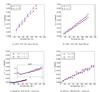 |
Fig. 2 Top: relative variation of spot width as a function of spot peak flux on CCD E2V-250 at two wavelengths, 550 nm (left panel) and 900 nm (right panel). Bottom left: MegaCam difference of second moments of stars to the average as a function of peak flux. Bottom right: same measurement on DECam CCD (S11). A small color correction is applied in both cases. One notes that in all cases the size increases linearly with the peak flux. |
The top panels of Fig. 2 show measurements performed on CCD E2V-250 with 550 nm (left) and 900 nm “star like” spots (right). In both cases, a linear increase of spot size with flux is visible. From a vanishing spot to saturation, it amounts to about 3.5% for the 550 nm spots and 2.5% for the 900 nm spots. The red spot reference size (which we define as the intercept of a linear fit) is ≈2 pixels, while the blue spot is ≈1.6 pixel. This difference is due to diffraction in the illumination setup. Since the spot sizes are different, we do not draw a conclusion on any wavelength dependence from these two data sets.
The MegaCam images exhibit an apparent increase of stellar PSF by about 0.008 pixel over the whole brightness range, which is approximately 0.5% for this sample (Fig. 2, bottom left). It should be noted that this range corresponds to half-filled CCDs (Borgeaud et al. 2000), due to the gain setting of the camera read out electronics. In this r-band on-sky data, we find that the increase rates are similar along rows and columns with a mild indication that it might be slightly larger (10 to 20%) along columns. This plot takes into account the relation that exists between the stars apparent size and color. The size-color relation is estimated using a set of low flux stars, in practice, where a small bin contains a large number of stars. The relation between the second moments, and the g − i colors is fitted by a linear relation. This polynomial is then evaluated for each star and substracted to its second moment. This method to subtract the size-color relation is replicated from Astier et al. (2013, Sect. 10).
The bottom right panel of Fig. 2 illustrates the effect as seen on DECam images using r-band images on CCD N17. Average PSF here is σx ≈ 1.7 pixel and σy ≈ 1.9 pixel. It exhibits a broadening of ≈2% from zero flux up to full well, which is slightly lower than what is observed on the CCD E2V-250. The size-color relation is taken into account, but its contribution is negligible. Over the chips of the focal plane, the average and spread of the brighter-fatter effect is (0.0250 ± 0.0040) [pix/100 ke−] in the X (serial) direction and (0.0252 ± 0.0037) [pix/100 ke−] in the Y (parallel) direction. The precision of this measurement for a single amplifier is ≈0.0010 [pix/100 ke−] in both directions, which is at least three times lower than the spread of the distribution for the entire camera: this may indicate small individual differences among sensors of the same model or small differences in operating voltages from sensor to sensor. This could also come from inaccurate gain estimations.
The comparison of the absolue amplitude ot the brighter-fatter effect found on the different sensors is summarized in Table 1. The projections in the X and Y direction are indicated in the first and second columns, respectively. For the CCD E2V-250, the slopes are found to be larger in the Y direction: by 15% at 900 nm and by 10% at 550 nm. The observation is more significant at 900 nm (10σ) than at 550 nm (2σ) due to a higher statistics. For DECam and MegaCam, the effect is also observed to be slightly bigger in the Y direction.
Comparison of the brighter-fatter effect in the X and Y direction that are observed on CCD E2V-250, DECam and MegaCam.
Figure 3 gathers relative size changes from the whole DECam mosaic dispersed as a function of IQ. It shows the maximum amplitude of the variation in the (g, r, i, z, Y) DECam filters. On the top panel, it can be noted that the relative amplitude of the effect becomes steeper when the IQ improves. On the bottom panel, data points from the various passbands are represented without normalization. It shows that the absolute amplitude of the broadening is actually quite independent of the IQ. It also indicates that the effect is mostly achromatic. Since it is also reported in Astier et al. (2013) that brighter-fatter slopes are consistent across bands for MegaCam sensors, it supports the observation that the effect is largely wavelength independent.
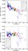 |
Fig. 3 Top: maximum (50 kADU) relative amplitude of the brighter-fatter effect in DECam. The relative slope becomes steeper when the IQ improves. Bottom: maximum amplitude of the variation of PSF shape in the various filters. The brighter-fatter effect seems achromatic, and the linear IQ increase seems fairly independant of IQ. |
To summarize, the brighter-fatter effect has been detected on all the CCDs that we have analyzed. Even though it is a small effect (few percent of PSFs mean width), it is quite easy to measure its amplitude with a few percent uncertainty. At this level of precision, no chromaticity dependence is seen, and a slight anisotropy in X and Y direction is observed.
4. Pixel spatial correlation in flatfield images
The broadening of spots with increasing flux presented in the previous section can be depicted as a reduction of the image contrast. We see in this section that a similar contrast reduction also appears in flatfield images. It manifests itself as a non-linearity of the photon transfer curve (PTC). A PTC is the representation of the variances versus the average fluxes of flatfield illuminations obtained with increasing exposure times. Considering only Poisson noise, the relation between the two observables is expected to be linear. However, we see that a significative departure from linearity is actually observed and that it is associated with linearly increasing pixel correlations.
4.1. Non-linearity of the photon transfer curve (PTC)
The non-linearity of the PTC is illustrated in Fig. 4 using eight different segments of the CCD E2V-250. The raw PTCs (on left panel) can be rescaled (on right panel) using a classic method with linear fit of the PTC at low flux level to determine the read out gain from the relation:  (1)where G is expressed in (e−/ ADU). When PTCs are rescaled to the same slope at the origin, the non-linearities clearly appear and are found to have similar magnitude in all channels (Fig. 4, right panel). When the residuals of the PTCs to the Poissonian noise are represented (Fig. 5), it is also seen that the phenomenon does not occur at a given threshold, but rather sets on from the very beginning of the PTC.
The non-linearity of the PTC is an unexpected feature: flatfield images are naively expected to exhibit a Poissonian noise, which is a variance scaling with the average. However, the variance measured at high-flux is actually significantly lower than expected from extrapolating the variance of low-flux flatfields according to Poisson law: the discrepancy is as high as 20% in the case of the CCD E2V-250. This effect has long been observed on other CCDs (Downing et al. 2006), but we have not been able to find a physical explanation in the literature.
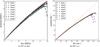 |
Fig. 4 a) Measured photon transfer curve of amplifiers #1 to #8 of the CCD E2V-250 expressed in ADU. b) PTCs are converted in e− using the readout gain measured as the inverse of the slope at the origin (see Sect. 4.3). Because departure from linearity of the PTCs is similar for different amplifiers this indicates that the cause of the effect is to be found in the CCD itself rather than in the electronic readout. |
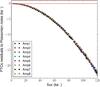 |
Fig. 5 CCD E2V-250: Residuals of the PTCs to the expected Poissonnian noise. The departure from linearity starts from the very beginning. |
4.2. Measuring pixel spatial correlations
4.2.1. Pair images subtraction
Correlation coefficients are computed from the difference of two flatfield images that have received the same overall illumination. This is a classic technique to remove apparent correlations due to non-uniformity of the flatfield image that is typically due to pixel size variations, QE variations, or spatial variations of the illumination itself. Temporal stability of the light source at the per mil level is then mandatory. In this analysis, this is why flatfields from artificial sources are being used rather than twilight flatfields.
4.2.2. Statistical precision
Spatial correlations between pixels are evaluated using covariances normalized by variance. Rk,l refers to the correlation coefficient between pixels separated by k columns and l rows. It is important to emphasize that k and l do not refer to independent variables but index the spatial relation between two pixels, so Rk,l ≠ Rl,k. The statistical precision on any given correlation coefficient is  , where N is the number of pixels. The statistics is doubled for the off-axis correlations (k,l ≠ 0) by combining the measurements of two quadrants (Rk,l and Rk, − l for instance). On MegaCam and DECam, each amplifier channel has 4 MPix while CCD E2V-250 reads 1 MPix per amplifier channel. This gives uncertainties of 0.5‰ and 1‰ respectively. Statistical precision is further increased by using many pairs of flatfields. The PTC from the CCD E2V-250 contains ≈100 points, which allows us to improve precision on correlation measurement down to 1 × 10⁻⁴. A smaller improvement is obtained in the case of DECam and MegaCam, where PTCs were acquired in situ, and gather only ≈20 points. The precision on correlation measurement on MegaCam is also reduced due to a partial readout of each channel (only 100 kPix). Anyhow, measuring pixel spatial correlations requires some care due to the existence of miscellaneous effects that generate spurious pixel correlations.
4.2.3. Spurious pixel correlations
Wherever hot or dark columns are being detected, they are masked. Moreover, CCD images sometimes exhibit localized image contrasts that are not attributed to the illumination itself but rather to CCD defects or to specific setups (clocking voltage (CV) and backside substrate (BSS) voltage) of the controller used to drive the CCD. They necessitate an elaborated masking algorithm, since the level may be very close to mean illumination and the patterns are multiforms. First, we detect the pixels that are 3σ above a local average1. Then, these pixels are masked if there are more than two other pixels above 3σ in their ±1 pixels surrounding. These masks are applied on both images from a pair and on its difference.
Correlations that cannot be attributed to any specific feature in the image can be otherwise detected from a non-zero intercept when fitting a given correlation coefficient versus flux. For instance most channels have more than 3σ residual anti-correlation R1,0 at zero flux in our LSST data set, while all the other coefficients have values compatible with zero. Considering that this offset is only affecting consecutive pixels in the readout sequence and that it manifests itself even without illumination, we assumed that it is introduced by the readout sequence (because of an incomplete reset of the baseline, for instance). Such an effect would generate linearly increasing covariances with flux, which translate to a constant correlation contribution that is subtracted from all measurements of R1,0.
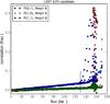 |
Fig. 6 Superposition of the evolution with flux for nearest pixel correlations (coefficients R0,1R1,1R1,0) for read out channels 1 to 8 of CCD E2V-250. The whole dynamical range shows a threshold where correlations strongly increase: first R0,1, a correlation in Y direction, and near full well, R1,0, a correlation in X direction. The diagonal correlation R1,1 does not exhibit any threashold. This is expected since neither transfer nor read out could contribute to correlate pixels in this direction. The vertical dark line indicates the early threshold of R0,1. |
4.2.4. Correlations at the high-flux level
On the high-flux end of the dynamic range, correlation features are expected to appear when the pixel contents are approaching full well. These are seen as blooming effects that increase up to saturation. These correlations have a characteristic signature: they appear when a given threshold is reached (that varies slightly from one read out channel to the other), first in Y direction, then in X direction and in diagonal but with a much smaller amplitude in the latter. Figure 6 illustrates these three features with the CCD E2V-250: R0,1 (in red) coefficient greatly increases at levels between ~130–160 ke−, depending on the amplifier channel. Near the full well, strong horizontal correlations R1,0 are visible (blue triangles). Lastly, the correlation R1,1 (in green) shows a quite linear behavior up to full well. Seen from this perspective, the dynamic range is not simply divided into two regimes with a low range, where pixels linearly respond to illumination, and a high range near full well, where pixels saturate. For this CCD, an earlier threshold occurs around 130 ke−, where R0,1 abruptly increases. It also corresponds to the extremum of the PTCs (Fig. 4). In the next section, we focus our analysis of pixel spatial correlations on the dynamic range below this flux level (indicated by the vertical dark line in Fig. 6).
4.3. Linearly increasing pixel spatial correlations
4.3.1. Pixel correlation maps
Pixel spatial correlations are detected on the three instruments up to a distance of 4 pixels. They are presented for CCD E2V-250, DECam, and MegaCam on Fig. 7. For LSST and DECam, the correlation R0,1 is about three times larger than R1,0, while they are of the same order for MegaCam. In all cases, this anisotropy between (Y) direction and (X) direction vanishes at larger distances. At a separation of 4 pixels, all correlations of all CCDs are as low as a few 10-4, which approaches the limit of sensitivity of the measurements.
For the CCD E2V-250, it has been shown by Antilogus et al. (2014) that an increase of the parallel clocking voltage (CV) from 8 V to 10 V decreases the level of the correlation R0,1 while keeping the other coefficients unchanged. In this paper, we complete the study of the impact of varying pixels’ electrodes voltage by repeating the measurements of the correlations with various backside substrate (BSS) voltages. The correlation with the next pixel in the parallel direction R0,1 (top panel of Fig. 8) increases as the BSS is decreased down to 10–20 V; below this level, the correlation starts decreasing. On the same interval, the correlation coefficient with next pixel in the serial direction R1,0 (middle panel) decreases and shifts to negative values below 10–20 V. The other correlation coefficients monotonously increase as BSS decreases (the bottom panel of Fig. 8 illustrates this with R0,2 and R2,0); it is worth noting that diffusion mechanisms (as suggested in Ma et al. 2014) cannot explain the evolution with BSS and CV, the amplitude, the anisotropy, and the long range of these correlation coefficients. In contrast, the predictions from a simple electrostatic simulation are compatible with these observations (see Sects. 5.1 and 5.3).
 |
Fig. 7 2D correlation map in flatfields at a 50 ke− level for a) CCD E2V-250 (channel 4, the channel on which spots illumination presented in the first section were done); b) DECam (CCD S11); and c) MegaCam. Row and column, respectively, correspond to label X and Y. An anisotropy between the amplitudes of the R0,1 and R1,0 coefficients is observed. For distance separations larger than 1 pixel, this anisotropy tends to vanish (RX,Y ≈ RY,X for X and Y > 1). |
The pixel correlation maps are found to scale with fluxes for all detectors. This is illustrated in Fig. 9 by zooming on the range 0 to 130 ke− for the eight channels of the CCD E2V-250 that were presented in Fig. 6. There is no evidence for chromaticity dependance of this general trend: a linear fit of Rk,l variations for PTC ramps obtained with illumination at 500 nm, 700 nm, and 900 nm wavelengths has shown no evolution with respect to wavelength. For instance R0,1 slope is found to be (1.39 ± 0.04) × 10-6 [frac/ADU] at 500 nm wavelength, (1.39 ± 0.04) × 10-6 [frac/ADU] at 700 nm wavelength, and (1.42 ± 0.03) × 10-6 [frac/ADU] at 900 nm wavelength. They are all compatible within 1σ rms; likewise, other correlation coefficients have no detectable variation either.
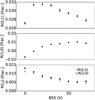 |
Fig. 8 Variation of correlation coefficients (measured at 100 ke−) with respect to BSS measured on the CCD E2V-250. Top panel: R0,1. Middle panel: R1,0. Bottom panel: R0,2 and R2,0. The other long range correlations behave like R0,2 and R2,0: they decrease as the BSS voltage increases. |
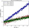 |
Fig. 9 Superposition of evolution with respect to flux of coefficients R0,1R1,1, and R1,0 on the dynamical range below the threshold, as indicated by the vertical black line of Fig. 6. On this interval, all the linearly increasing correlations that are discussed in this section shows a monotonic behavior. On this CCD E2V-250, most channels exhibit a small (≈–0.003), but significant anti-correlation pedestal in R1,0 (Y-intercept), an offset that is not seen with the others coefficients nor with the other sensors. We attribute it to the electronic chain used to collect this data, and we subtract it to the actual measurements. |
4.3.2. Relation between PTC non-linearity and linearly increasing correlation
It has been verified that the process that correlates the pixels also conserves charges. This is straightforward to see from a linear fit of flatfield mean flux versus exposure time. For instance the departures for the eight channels of the CCD E2V-250 from linearity of response on the range from 0 to 130 ke− are below 2‰ peak to peak.
The connection between non-linearity of the PTC and the linearly increasing correlations can be most clearly illustrated by summing all the correlations and adding them to the PTC. In Appendix A, we assume a conservation of charge to demonstrate that the difference between the raw PTC and the Poisson variance is the sum of the covariances. This conclusion has a consequence on the measurement of the gain that was given by the relation (1). It is then modified in the following way:  At this point, α is an empirical parameter that is introduced to describe the quadratic behavior of the PTC, which is expected given a linear rise of the correlations. We refer to the end of Sect. 5.2 for an interpretation of this parametrization using our model. The variable G is obtained by a second degree polynomial fit on a range up to the PTC extremum, instead of the linear fit on an arbitrary low flux interval. It should be pointed out that the gain discrepancy between both methods can be as large as 10% depending on what is assumed to be the low flux interval. For this new method, the relative uncertainty on the gain estimation is found to be between 3–4‰ half of which comes from shot noise, while the rest corresponds to the 2‰ departure from linearity of response.
Figure 10 shows that the linearity of the PTCs are restored when the variance and the covariances are added together. The plot is expressed in e−, using the gain as measured by the method presented above. At a 100 ke− flux level, the covariances (up to 4 pixels in distance) add up to 18% of the variance. The dashed red line that appears on the plot indicates the expected photon noise. Its slope is ≈0.5% above the combination of variance plus covariance, which is consistent with a truncation of the sum of small residual correlations at distances larger than 4 pixels. It indicates that they correspond to less than 3% of the total pixel correlations.
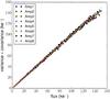 |
Fig. 10 Comparison for the CCD E2V-250 between the expected Poisson noise (red dashed line) and raw PTCs that are corrected by summing covariances up to 4 pixels distance. For a 100 ke− flux level, these correlations add up to 18% of the variance. The corrected PTCs slopes coincide with Poisson law at ≈0.5%, indicating that more than 97% of the correlations are considered by the truncation at a 4 pixels distance of the integral of the correlation function. |
4.4. Summary of correlation properties
Linearly increasing correlations are seen on all tested CCDs. They are the origin of the quadratic behavior of the PTC. It requires care to precisely separate them from other already identified correlating processes, but then they are detected up to 4 pixels distance at a level of a few 1 × 10⁻⁴. We propose in the next section a physical source of these correlations that is also found to generate a broadening of spot-like illumination.
5. A simple model of Coulombian forces within CCDs
We propose an explanation for both the brighter-fatter effect and correlations in flatfields, which involves transverse field line displacements due to charge distribution within surrounding pixels. With a simple electrostatic simulation, we evaluate how much it would affect spot broadening and pixel correlations. We further derive a simple model that uses correlation measurements to predict brighter-fatter relations.
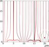 |
Fig. 11 Electrostatic calculation of Coulombian forces generated by the electrode voltage (CV), the depletion voltage (BSS), and the electrons collected. This figure is a zoom of the last 20μm of 100μm thick simulated pixels. The black lines represent the electric field for empty pixels, and the red lines represent the electric field when the right most pixel is filled with 50 ke−. The separations between two adjacent pixels are indicated by the bold lines and are shifted to the right when adding the charges. This results in a variation of pixel effective size: the size of the filled pixel has decreased, while the size of neighbor pixel has increased (and its centroid has slightly shifted). This figure also qualitatively confirms the observation that the effect is achromatic: we see that drift trajectories are altered in the bottom ~10μm of the device only, and hence do not depend significantly on the conversion depth. |
5.1. Evolution of electrostatic fields as charges accumulate into pixels
Combining the observation of correlations in flatfield images with the broadening of stars with flux, we picture the effect that the charges accumulated in a CCD perturb the drift electric field that subsequent charges will experience. These perturbations tend to drive drifting charges away from pixels with higher counts than their surroundings. In flatfield images, these higher counts result from Poisson fluctuations, while they result from genuine illumination variations in star or spot images.
The relevance of this description has already been assessed in Antilogus et al. (2014) by showing that a simple electrostatic simulation of the pixels reproduces both the brighter-fatter effect and the scale of pixel correlations. Figure 11 illustrates the phenomenon at play by superposing the electric field lines for empty pixels and for a pixel that is filled with 50 ke−. In this simulation, the pixel geometry correspond to the CCD E2V-250, and we approximate the intrinsic silicon as free of charges. The CCD is simulated with a bias voltage (BSS) of 70 V, a clocking voltage (CV) of 10 V, and a depth where charges accumulate of 2.5μm. The same electrostatic potential that separates pixels in rows is applied to the column separation (because we do not know the exact profile of the implants that define the column separation). The pixels boundaries are found by following field lines from the top to the bottom of pixels. The figure illustrates that these boundaries are displaced by the charge pattern stored in the device. The sense of the effect (due to repulsion of same sign charges) is that pixels with higher counts than their surroundings shrink as they fill up, while their neighbors widen and slightly shift. The figure also illustrates that the second neighbor pixel is also affected. The consequence of this evolution of the pixel effective size2 is that pixel correlations in flatfield images should increase with increasing fluxes and that point sources should appear broader as they get brighter. The photon noise that contributes to the contrast of a flatfield is reduced as drifting charges are being more repelled by a pixel where more charges have already accumulated. Meanwhile the perturbation of field lines in the surrounding of a spot in an astronomical image results in a broadening of its width as the source becomes brighter.
The agreement that was found between the simple electrostatic simulation and the observations is only qualitative, and a quantitative prediction would necessitate a detail knowledge of the geometry of the CCD and of the doping that are not available. To test the quantitative prediction, we have developed a generic model that describes both effects with the same algebra.
5.2. Empirical parametrization of the pixel size variations as a function of flux
In this section, we derive a parametrized model of the effects of electric field distortions in a CCD that are induced by the charges residing within the CCD during the exposure. We model the displacement of the effective boundaries of a pixel (labeled (0,0)), which is caused by a charge qi,j in a bucket at position (i,j) as 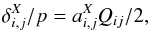 (2)where we have expressed that the (perturbing) electric field due to a charge is proportional to this charge (Qij), and approximated alterations to drift trajectories to first order. The variable p refers to the pixel size, and we have introduced a factor of two for convenience. The variable X indexes the four boundaries of the pixel (0,0), and we label each boundary by the coordinates of the pixel that shares it with (0,0): X ∈ {(0,1), (1,0),(0, −1), (−1,0)}. The
  coefficients that define the model3 satisfy symmetries
 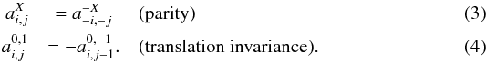 Each boundary of the pixel (0,0) shifts under the influence of all charges. Its displacement reads
 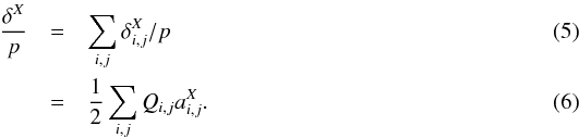 If all charges qi,j are equal, the electric field induced on a pixel boundary vanishes, and the boundary does not shift. As a consequence, the have to obey sum rules:
 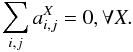 (7)We call charge transfer the difference between charge contents with and without the perturbing electric fields. The displacement of the pixel boundary δX induces a charge transfer between the pixel (0,0) and the pixel X, where X ∈{ (0,1),(1,0),(0, −1),(−1,0) }. To first order, this charge transfer is proportional to both the pixel boundary displacement and to the charge density flowing on this boundary. For a well-sampled image (i.e. the charge distribution impinging a pixel does not vary rapidly within this pixel), we can approximate the charge density drifting on the boundary between pixel (0,0) and its neighbor X as
 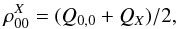 (8)so that the net charge transfer due to perturbing electric fields between pixel (0,0) and its neighbor X reads
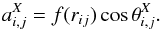
 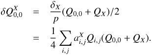 (9)The expression is non-linear with respect to the charge distribution: the charge Qi,j is the source charge, and the expression (Q0,0 + QX) approximates the test charges. A calculation of
  boundary displacements resulting from a spot having 100 ke− in pixel maximum and a Gaussian shape with a rms of 1.6 pixel is given as an illustration Fig. 12. The net charge transfer within the central pixel results in a decreasing effective size, while the effective size of pixels away from spot center tend to grow.
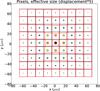 |
Fig. 12 Illumination with a spot having 100 ke− in pixel maximum and a Gaussian shape with a rms of 1.6 pixel results in boundary displacements (multiplied by a factor 5, red lines) that depend on the distribution of charges within surrounding pixels (colored circles). The displacements between the intial boundaries (black) and their final positions (red) correspond to the δX terms of our model. It shows that the central pixel effective size shrinks as illumination increases, while pixels away from spot center tend to grow. |
When dealing with electrostatic simulations, we have to account for the charge build-up during integration: on average the perturbations to the drift electric field are over the exposure time half of what they are at the end of the exposure. This justifies the factor of 2 in expression 2, so that the  coefficients can be extracted from simulations as the ratio of the boundary displacement (in pixel size unit) to the source charge.
The perturbed charge in pixel (0,0) reads  (10)with
  (11)To evaluate the statistical correlations introduced by the charge-induced perturbations of drift trajectories, we wish to evaluate
 ![\begin{eqnarray} \label{eq:cov_2} {\rm Cov}(Q'_{i,j}, Q'_{0,0}) &=& {\rm Cov}(Q_{i,j}, \delta Q_{0,0}) + [(i,j)\leftrightarrow(0,0)] + O(a^2) \nonumber \\ &=& 2{\rm Cov}(Q_{i,j}, \delta Q_{0,0}) + O(a^2), \end{eqnarray}](/articles/aa/full_html/2015/03/aa24897-14/aa24897-14-eq85.png) (12)where O(a2) stands for expressions quadratic in the coefficients of expression 9. We stick to first order perturbation expressions, as real data indicates that this is justified. In the case where the pixel (i,j) is not a nearest neighbor of (0,0), we have
(12)where O(a2) stands for expressions quadratic in the coefficients of expression 9. We stick to first order perturbation expressions, as real data indicates that this is justified. In the case where the pixel (i,j) is not a nearest neighbor of (0,0), we have ![\begin{equation} {\rm Cov}(Q_{i,j}, \delta Q_{0,0}) = \frac{1}{4} {\rm Var}(Q_{i,j}) \sum_X a^X_{i,j} E[Q_X+Q_{0,0}], \end{equation}](/articles/aa/full_html/2015/03/aa24897-14/aa24897-14-eq87.png) (13)which for a flatfield illumination of average content μ and variance V reads,
(13)which for a flatfield illumination of average content μ and variance V reads, 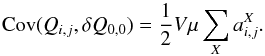 (14)In case the pixel (i,j) is a nearest neighbor of pixel (0,0), say Y, we have two terms in the covariance4:
 ![\begin{eqnarray} {\rm Cov}(Q_Y, \delta Q_{0,0}) && \simeq \frac{1}{4} {\rm Var}(Q_Y) \sum_X a^X_Y E[Q_X+Q_{0,0}] \notag\\ &&\quad + \frac{1}{4} \sum_{i,j} a^Y_{i,j} {\rm Var}(Q_Y) E[Q_{i,j}]. \end{eqnarray}](/articles/aa/full_html/2015/03/aa24897-14/aa24897-14-eq91.png) (15)For a flat, the second term vanishes because of the sum rule (Eq. (7)). So, using Eq. (12), we find that whether or not (i,j) is a nearest neighbor, the covariance between pixels in a uniform exposure of average μ and variance V reads
(15)For a flat, the second term vanishes because of the sum rule (Eq. (7)). So, using Eq. (12), we find that whether or not (i,j) is a nearest neighbor, the covariance between pixels in a uniform exposure of average μ and variance V reads 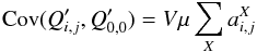 (16)to first order of perturbations. The electrostatic influence from collected charge, thus, induces covariances between pixels in uniform exposures that scale with the average and the variance of pixel contents. If one measures correlation coefficients (ratio of covariance to variance), those are expected to scale with the illumination level of the uniform exposure. In the same manner, applying this equation to (i,j) = (0,0) and replacing in the expression (10), it shows that our model of electrostatic influence also predicts a quadratic behavior of the PTC:
 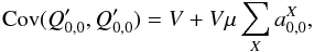 (17)which allows us to identify the α term from the equation Sect. 4.3.2 as a combination of the a00 parameters:
 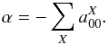 We notice that α is positive because the four
  terms are negative (they correspond to the narrowing of a pixel due to one collected charge within).
Ma et al. (2014) propose a model, which corresponds to a peculiar solution of Eq. (16)where all the of a given pixel are set equal. This parametrization totally contradicts the findings of Sect. 5.1 (see for instance Fig. 11). They refer to their model as a “charge-sharing” phenomenon. It follows a proposition from Downing & Sinclaire (2013), who report a variation of the non-linearity of the PTC when varying the collection phase voltage and who interpret it as a consequence of the variation of the lateral diffusion. It should be noted that lateral diffusion variation cannot be evocated without the fact that mean trajectories are also modified. We show in the next section that this diffusion is a sub-dominant contribution for the brighter-fatter effect.
5.3. Influence of diffusion in the substrate
Although diffusion actually smooths charge distributions, it is not the best candidate to explain the brighter-fatter effect or correlations in flatfields. The diffusion equation is linear and hence is not obviously well suited for describing a linearity-violating phenomenon, such as the brighter-fatter effect. Diffusion also does not cause correlations between pixels as long as the probability to convert in a given pixel and be collected in some other pixel does not depend on the pixel contents. These are first order arguments because diffusion indeed contributes to both the brighter-fatter effect and correlations and because the charge contents alter (indeed reduce) the longitudinal drift electric field on which the diffusion coefficient depends. The mechanism is thus the following (Holland et al. 2013): a pixel with higher counts than its surroundings will have a lower drift electric field than its neighbors (see e.g. Kent 1973), and the increased diffusion will increase in turn the probability of transferring photo-electrons to neighboring pixels.
The impact of diffusion to transfer charges across pixels can be sketched to first order of perturbations: a charge stored in the CCD will alter the probability that electrons converted above a pixel diffuse to a neighboring pixel. To first order, this probability is proportional to the source charge, and the amount of transferred charge via this mechanism follows the expression (9), although we had invoked boundary displacements to justify it. So, our model from Sect. 5.2 is actually fully compatible with this second order effect of diffusion. We, hence, expect that the latter does not break the relation established by our model between correlations and the brighter-fatter slope. We can, however, readily note that since the contribution of diffusion depends on the conversion depth (which varies on average with wavelength), the fact that we do not observe a significant chromatism of the effects indicates that this second order contribution of diffusion is modest. It is nevertheless interesting to evaluate its contribution to the overall broadening of spots or stars, for example to assess the impact of ignoring it in the outcome of electrostatic simulations.
We have hence evaluated the contribution of the variations of diffusion induced by the charges stored in the CCD to the brighter-fatter effect, using the following assumptions:
-
Lateral diffusion causes a spot broadening that is
 , where tr is the transit time.
 -
Transit time is estimated by
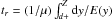 , assuming that charges velocity is v = μE(y).
 -
The variation of the “instrumental” PSF (
 ) is then computed using our electrostatic simulation starting with empty pixels and adding charges up to 100 ke−.
 -
For DECam, we use its nominal backside substrate voltage and clocking voltage parameters: a BSS of 40 V and a CV of 6.5 V. For CCD E2V-250, we use the values applied to acquire these data sets: a BSS voltage of 70 V and a clocking voltage of 10 V. The pixel thickness (Z) and width are as indicated by manufacturers. The depth of the buried channel, which is the only free parameter ot the simulation, is set to 2μm.
Our results are summarized in Table 2. For a device operated at low drift field, such as DECam (E = 0.16 V/μm), we find that the variation of lateral diffusion is ~20%. Given that the contribution to the broadening is half the maximum variation, it contributes to ~10% of the brighter-fatter slope (for realistic IQ conditions), while the contribution is no more than a few % of the observed brighter-fatter slope for the higher drift field (E = 1 V/μm) that is used to operate the CCD E2V-250. So, this effect alone does not quantitatively match the measurements reported in Sect. 3.3. It even appears to be secondary when simulating “high-field” devices (such as presented in Sect. 5.1) for which simulations accounting for the alterations to the average drift trajectory might be sufficiently accurate. In any case, the applicability of the parametrization that we present in Sect. 5.2 does not depend on a detailed description which separates the relative contributions of lateral and of longitudinal electric fields to the charge transfers: the outcome of our correction method is relevant for a physical interpretation that is a combination of both diffusion and drift of the electrons.
Upper limit of diffusion variation for CCD E2V-250 illuminated by 550 nm spots and for DECam CCD N17 in r-band.
6. Connecting flatfield correlations with the broadening of spot-like illumination
For CCD E2V-250, DECam, and MegaCam, we compare the brighter-fatter slopes expected from the correlations measured in flatfield exposures with the brighter-fatter slopes measured directly. The first step is to derive the values of the model coefficients from the correlations. By using the found coefficients, the second step is to emulate the electrostatic distortions by transforming images of faint spots into realistic bright spots and compare those with real bright spots.
6.1. Extracting the model coefficients
The coefficients are determined from the correlation coefficients Ri,j. They are extracted from correlation slopes fitted on flatfield pairs up to PTCs extremum. We have measured correlations up to 4 pixel separation, which is 25–1 measurements, or n2−1 for n = 5. Each pixel has 4 boundaries; there are 4 × n2 coefficients to be determined. With n = 5, there are 100 boundaries to consider. The internal consistency of the model directly removes the calculation of 40 boundaries that are shared by two pixels. The parity of the effect (Eq. (3)in Sect. 4.3.1) also removes ten boundaries that are mirror of one another as seen from the source charge (5 in i and 5 in j). So we are left with 2 × n2 (50) coefficients to evaluate.
There are n2−1 measured correlations (related to coefficients by Eq. (16)in Sect. 4.3.1), and we complete those by n2 + 1 extra constraints in order to have a closed system. We derive the needed constraints from smoothness considerations: the measured correlations decay smoothly with distances and so should the coefficients. We will first derive a crude model for these coefficients from the measured correlations, and then use this model to constrain ratios of at similar distances, and constrain values at the farthest boundaries. We then directly solve and assess how our predictions for the brighter-fatter slopes depend on the intermediate smoothing model used.
The smoothing model assumes that coefficients are the product of a function of distance from the source charge to the considered boundary (rij) and that it also trivially depends on the angle between the source-boundary vector and the normal to the boundary ( ):
):  We have tried various analytic forms for f(r) and settled for the exponential integral function:
 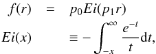 (18)where Ei is only defined for x> 0 and the singularity of the integrand around t = 0 is handled by taking the principal part. We determine p0 and p1 by least-squares:
 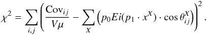 Because we observe anisotropic correlations at short distances (e.g. Cov01 ≠ Cov10), we do not include the three nearest neighbors in the fit. The fit to the 21 other correlations is shown in Fig. 13 with the minimization values. The agreement justifies the choice of the exponential integral function.
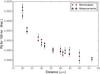 |
Fig. 13 Correlation coefficients of the non-nearest neighbors for the CCD E2V-250 are represented as a function of their distance (black triangles) and the correlation coefficients reconstructed from a χ2 minimization (red circles) using an Exponential Integral function. This function is used to estimate the last boundaries displacement. |
We use the fitted p0 and p1 parameters to impose the values on the farthest boundaries (2 × n constraints) and also to impose ratios of coefficients addressing adjacent boundaries of the off-axis coefficients (i.e. i,j> 0). It reads 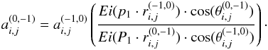 No constraints are applied on the displacement of the boundaries of the pixels (1,0) and (0,1) because the analysis of correlation properties presented in Sect. 4.3.1 indicates a different behavior for those than for the rest of the coefficients. The displacements of the boundaries that are next to the source charge are due to a combination of effects: some of them being unknown (the actual geometry of the collecting area), other being complex (a contribution both from charges diffusion and from electrostatic influence (Sect. 5.3)). The solution of the model for all boundary displacements is represented by the red shaded area in Fig. 14. The width of the area corresponds to the propagation of the ±1σ uncertainty of the correlation coefficents measurement. It exhibits an irregular variation with distance that is introduced by the X/Y anisotropy in correlation coefficients, which is ignored in our simple simulation. Nonetheless, the overall shapes are compatible. To assess the sentivity of the results to the smoothing model we vary p1 by ±5σ, which changes the coefficients by about ± 1%. This in turn changes the brighter-fatter slope by about 3 × 10⁻⁴.
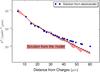 |
Fig. 14 Boundary displacements ( |

6.2. Image sampling and estimates of perturbed charges distribution
The last step to emulate the electrostatic distortion is to multiply boundary displacement with charge density flowing on boundaries. Assuming that the image is properly sampled, the density is approximated by interpolating among the pixel contents (Eq. (8)). The accuracy of this approximation can be estimated by the simulation of spots with increasing size using Moffat functions. The exact charge density is then known everywhere in the images and, in particular, on the pixel boundaries. The result of the test is shown in Fig. 15 for the IQ ranging from 1.2 pixel to 3.5 pixels. For an IQ of 1.6 pixel (such as our 550 nm spots on the CCD E2V-250), with a relative brighter-fatter effect of ~2%, the approximation introduces an underestimation on the size of the spot that is already below 0.1%, which is less than 5% of the amplitude of the effect.
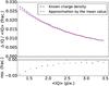 |
Fig. 15 Top panel: IQ variation for 100 ke− (peak) spots after having redistributed the charges (on a range comparable to what was presented for DECam on Fig. 3). The accuracy of the approximation of the interpolation method (in red) is compared with the result found using the exact charge density (in blue). Bottom panel: residuals. For an IQ of 1.6 pixel, such as 550 nm spots on CCD E2V-250, the approximation introduced an underestimate below 0.1% on the size of the spot, which is less than 5% of the amplitude of the effect. |
6.3. Comparison of the redistribution model with the measurements
The redistribution of charges in spot/star images consists of
-
1.
Establishing a low flux spot/star model from images of faint spots in the case of CCD E2V-250 and a fitted PSF model using astronomical images in the case of DECam and MegaCam.
-
2.
Scaling up the image flux by the desired factor.
-
3.
Transforming the image through Eq. (11)(“redistribution”) from Sect. 6.1.
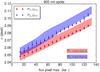 |
Fig. 16 Comparison between the broadening of spots from the redistribution and the data (CCD E2V-250, 900 nm spots). The ten low flux spots (≈13 ke−) are redistributed after increasing normalization to cover dynamical range (shaded areas). This shows the ability of our model of pixel effective size to reproduce the spot size increase observed in the brighter-fatter effect. |
6.3.1. Redistribution of charges for the CCD E2V-250 images
Redistribution of charges of low-flux 900 nm spots on the CCD E2V-250 does reproduce spot broadening with respect to increasing fluxes. This is illustrated in Fig. 16, where the redistribution of charges of low flux spots (shaded areas) is compared to the data (error bars represents ±1σ dispersion of measured second moments). It is seen that the trend is well reproduced both in X and Y directions. The constant width of the shaded areas originates in the initial dispersion of the 10 low flux spots (20 s exposure time, 13 ke− in maximum pixel). As for the data, the dispersion of the measurement of the second moments decreases as the S/N improves at higher fluxes.
We can also approximate the inverse of the transformation of Eq. (11)by using the same expression after flipping signs of the coefficients. This transformation reduces spot widths down to their low-flux sizes. The accuracy of the transformation is assessed by evaluating the residual dependence of the spot width on the spot flux over the dynamic range. This is shown in Fig. 17 for both 550 nm and 900 nm spots. The uncertainty of the result is indicated and separated between the statistical uncertainties that comes from correlation measurements and that are propagated using Monte Carlo simulations (plain colors) and the dispersion coming from second moment measurements (indicated in light colors). The dashed lines on the middle panel illustrates the results of reverse redistribution of charges when taking correlations up to 1, 2, 3, 4 distance into account. It reduces the brighter-fatter effect by 20%, 45%, 70%, and 87%, respectively. The relatively small contribution of the correlations from adjacent pixels emphasizes the importance of a long distance mechanism contributing to the brighter fatter effect. The bottom panel represents, for the 900 nm data set, the effect of the correction as a function of the distance in pixels, with the limit conditions for the taken into account. It indicates that there is no further evolution farther than the 4 pixel solution.
The slopes of spot broadening before and after reversing the broadening effect are summarized in Table 3.
The broadening of the 550 nm spots is measured with a ~3.6% relative precision on the X and Y slopes and with a ≈1.5% relative precision on the 900 nm spots. The reverse redistribution method is found to consistently remove the spots broadening and leaves no residual slopes to within 5% of the initial effect. It is below 1σ rms of the combined uncertainties, with the exception of the Y direction of the 900 nm spots for which it is below 2σ rms Although not significant, it should be pointed out that the amplitude of the residuals are compatible with the expected underestimation introduced by the charge density approximation (see Sect. 6.2). Lastly, we observe from Table 3 that for the 900 nm spots the errors on the correction are dominated by the model. It indicates that the ability to measure distant correlations (down to 1 × 10⁻⁴ level) is an essential step for an accurate application of this brighter-fatter correction method.
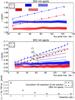 |
Fig. 17 Spot size along X and Y directions for 550 nm spots (top panel) and 900 nm spots (middle panel) on the CCD E2V-250. Raw spots are fitted with lines and measurements after redistribution of charges with the inverse model are shown with shaded area. Light colors correspond to dispersion coming from spot size measurements while darker colors represent the propagation of statistical 1σ uncertainties on correlations coefficients given that 50 pairs of flats were used. The five dashed lines on the lower panel indicate the redistribution prediction for the spot broadening in the Y direction when taking an increasingly large area of pixel correlations into account. It ranges from ±1 pixels distances to ±4 pixels and ±4 pixels plus the limit condition (4 + LC) established in the previous section. In the latter case, it is found that the correction restores the invariance of the PSF size with respect to increasing flux with a relative precision below 5‰ at 550 nm and 3.4‰ at 900 nm. The bottom panel represents the brighter-fatter effect as a function of the extension of the solution with the limit condition taken into account. It shows that the boundaries displacement at distance further than 4 pixels have a negligible impact on the solution. |
6.3.2. Redistribution of charges for DECam and MegaCam stars
The redistribution method also reproduces the amplitude of the effect measured on DECam but with less precision due to the limited number of flatfields in the publicly available science verification images. A comparison is shown in Fig. 18 with CCD-S11, using a set of 20 r-band exposures acquired in December 2012 (giving ≈13 000 stars). A PSF model is extracted from the set of images to serve as a spot reference. Charges are then redistributed after scaling up the spot reference in flux. A Monte Carlo simulations is used to propagate uncertainties from the measurement of the correlations to the prediction of brighter-fatter slope. On this CCD, it predicts a broadening of about 0.025 pixel between 0 and 100 ke−, which is symmetrical in X and Y direction. The rms from coefficient measurement uncertainties is 0.004 pixel at 100 ke−, which result in a 16% relative uncertainty on the modeling of the effect. This is near twice as much as for CCD E2V-250, and it is directly connected to our science verification data set that contains about four times fewer pairs of flatfields to estimate correlation coefficients. Nonetheless, the average value of the redistribution method reproduces the observations well, in both X and Y direction.
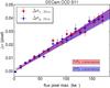 |
Fig. 18 Measured brighter-fatter effect and simulated effect seen on DECam CCD S11 and showing the propagation of correlation coefficient uncertainties. A ±1σ rms is 0.005 pixel at 100 ke−, giving a 25% relative uncertainty, which is slightly more than the dispersion measured on this stack of 20 astronomical images. |
When the comparison is performed on the whole focal plane, a 10% disagreement is found between the redistribution method and observations (Fig. 19). Prediction for average X and Y brighter-fatter effect for the entire camera are 0.022 pixel/100 ke− in both directions, while it is found to be 0.025 pixel/100 ke− in both directions from the observations. This discrepancy does not come from the color correction that is applied to decorrelate the second moments of stars from their color at fixed brightness. In the r-band, this correction is actually negligible (a 1 × 10-5 pixel/100 ke− decreasing of the average slope). The discrepancy is rather likely related to the non-linearity correction that has to be applied to the images: the average of DECam flatfield departs from strict proportionality to the exposure time by ~2%. If no corrections are applied, the average slope measurement is found to be 0.016 pixel/100 ke−. When the correction is applied at the pixel level to linearize DECam response to illumination, it shifts the average slope measurements to 0.025 pixel/100 ke− 5. With this level of non linearity, a careful handling is critical to obtain an accurate estimation of the brighter-fatter effect.
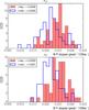 |
Fig. 19 Comparison of measured and simulated brighter-fatter slopes for DECam r-band. There are 57 CCDs over the 62 that are presented: we reject five CCDs for which at least one of its amplifiers has a reduced χ2 for the linear fit of the correlation R1,1 that is above 3. Astronomical images are being corrected at the pixel level to take non linearities detected from looking at flatfield mean fluxes versus exposure time into account. This increases the measured slopes by about 60%. While this correction is quite important, very small changes in the way non-linearities are fitted could account for the disagreement between measurements and model. |
The mean prediction of stellar image broadening in the X and Y directions for the 36 MegaCam CCDs is presented in Fig. 20 (shaded areas). The figure gathers the correlations from all the CCDs so as to palliate the lack of statistics coming from the small size of the frames in the flatfield data set. The relative uncertainty is still quite large at almost 50%. It is compared with a combination of all the epochs from the CFHTLS deep field (D1), which contains about 1.8 M PSF estimations and which result in a high precision measurement. At this level, very small effects show up, such as a small gap around 10 ke−, the origin of which is not fully understood yet. It should be remembered that the MegaCam brighter-fatter effect is already at a few per mil level (while it is at a few percent level for thick CCDs) and that the low-flux feature observed here is already at a 10-4 level.
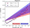 |
Fig. 20 Average brighter-fatter slope in the X and Y direction for the MegaCam mosaic. The observations gather all the deep field (D1) r-band images of the CFHTLS (≈1.8 M stars). The redistribution prediction is based on the mean correlations of all the CCDs; this is necessary to palliate the lack of statistics given the small frame of the flatfields data set. The prediction is compatible with the observations but with a significant uncertainty. |
In this last section, we have presented the precision that can be achieved on predicting the brighter-fatter effect using our model. The approximations that are made to tune the pixel effective size model are also presented, and their contributions to the systematics are evaluated. With the best quality data sample, as in the one from the CCD E2V-250, an agreement better than 5% is found between the prediction and the measurement. We have also shown that it can be used to reverse the redistribution of charges in pixels, which allows to decorrelate the measurement of PSF widths and fluxes. The precision that is reached is limited by the evaluation of the long range correlations. This indicates that the quality of the collected PTCs is currently the critical aspect to accurately correct for the broadening of point source image with increasing flux.
7. Conclusion
In this paper, we have studied two distinct effects that can be observed in CCD data in detail. The first one is the presence of long distance pixel correlations within flatfield images, whose amplitude increases linearly with flux (adding up to 8–18% for 100 ke− levels). These correlations explain the sub-Poissonnian behavior of the photon transfer curves (PTC), which has been long noted on multiple occasions by several authors. The second effect is the broadening of the PSF of stars with an increasing flux affecting spot/star images (0.5–3% for 100 ke− levels). This so-called “brighter-fatter effect” has been first observed on LSST sensor candidates, and has since been confirmed by other teams.
Using three different data sets collected with three different types of sensors, we have shown that long distance pixel correlations and PSF broadening are ubiquitous and seem to be a generic feature of CCD devices. They not only affect the modern totally depleted thick sensors, which equip/will equip DECam and LSST, but they are also detectable on the thin CCDs, which equip MegaCam.
We argue that pixel correlations and PSF broadening are deeply connected. Both effects can be described in terms of contrast reduction as a function of the flux stored in the pixels. Hence, we expect them to share a common physical explanation. We have developed a physical model to explain our observations. At the heart of this model is that the charges accumulated in each pixel produce an alteration of the electric field within the CCD. Therefore, the pixel boundaries, which are set by the drift field, evolve as the charges are being collected.
To test this explanation, we have performed an electrostatic simulation that calculates the alterations to the electric field within the CCDs, as charges are being collected. The outcome of the simulation can be pictured as a shift of the pixel boundaries that depends on its content and on the contents of the pixels in its surroundings. The model is able to reproduce (1) the long distance correlations observed in flat fields; (2) the broadening of the PSFs; and (3) the dependence of both on incoming flux and CCD operating voltages. In all cases, we find that the amplitude of the effects that are predicted by the simulation matches our observations.
Lastly, we have sketched a strategy to account for the brighter-fatter effect in a data analysis pipeline. The main challenge here is the precise characterization and modeling of the effect. A possibility would be to rely on extensive electrostatic simulations of the CCDs. This approach necessitates a detailed knowledge of the geometry of the channel stops and of the doping concentration to accurately predict the charge redistribution. This information, which is not usually available, would be required with high precision to be able to predict both the increase of the diffusion and the evolution of the drift lines of the electrons. The first effect is governed by the attenuation of the longitudinal field, which is a short distance contribution that is only affecting adjacent pixels. The latter contribution depends on both the longitudinal and the lateral electric field and extends up to several pixels separation.
Rather than a sophisticated simulation of charge trajectories, we propose an empirical model of dynamical charge transfers, which is tuned on the high quality measurements of correlations in flatfields. It is based on an algebra that connects the displacement of each given pixel boundaries to the correlations with the surrounding pixels measured on series of flatfields. The model is insensitive to the description of the electrostatic within the CCDs. The simultaneous determination of boundary displacements within a given map of pixels correlation is performed by setting (1) a limit condition on the correlations and (2) a relation between orthogonal boundaries. We find that this reverse redistribution method reduces the brighter-fatter effect by more than one order of magnitude. We conclude that the recovery of a flux homothetic PSF is currently limited in precision by the quality of PTCs associated with a given CCD, from the estimation of the errors that are introduced by our assumptions and from the propagation of the statistical uncertainties on correlation measurement.
We have not discussed how these corrections can be practically implemented in an image analysis pipeline. There seem to be at least two options. A first possibility is to apply a reverse redistribution correction at the pixel level, as done in this paper. Another is to incorporate the effect directly in the PSF model. The relative merits of these two approaches depends on the science goal (e.g., whether it is measuring fluxes or shapes). Deciding which is the best approach requires additional work, and we defer this discussion to later papers.
The accumulation of charges also modifies the effective size of the pixel because of an attenuation of the longitudinal component of the electric field, which causes an increase of the diffusion. This contribution is discussed in Sect. 5.3.
Compared to Antilogus et al. (2014), we have chosen a different normalization of the coefficients here, because the relation between electrostatic calculations and predicted effects is now straightforward.
The exact expression involves the third moment (or the skewness) of the charge probability density function, which is non-zero for a Poisson distribution. However, since we can approximate the statistics of pixel content with a Gaussian distribution, which has no skewness, this contribution of the third moment can be safely neglected. The relative error is of order 1/ ⟨ Q ⟩ with Q expressed in electrons.
Acknowledgments
The authors wish to thank Jean-Charles Cuillandre, Juan Estrada, Gary Bernstein, and Robert Lupton for useful discussions. The authors are grateful to the DES collaboration for acquiring and making available the DECam science verification data. We are also thankful to the LSST sensor team for providing the CCD E2V-250 data set.
References
- Amara, A., & Réfrégier, A. 2008, MNRAS, 391, 228 [NASA ADS] [CrossRef] [Google Scholar]
- Antilogus, P., Astier, P., Doherty, P., Guyonnet, A., & Regnault, N. 2014, J. of Instrumentation, 9, C03048 [Google Scholar]
- Astier, P., El Hage, P., Guy, J., et al., 2013 A&A, 557, A55 [NASA ADS] [CrossRef] [EDP Sciences] [Google Scholar]
- Bernstein, G. M., & Jarvis, M. 2002, AJ, 123, 583 1 [NASA ADS] [CrossRef] [Google Scholar]
- Bernstein, G. et al. 2013, in Precision Astronomy with Fully Depleted CCDs, in Prep. Proc. of Cosmo 2013 at BNL 2 [Google Scholar]
- Betoule, M., Kessler, R., Guy, J., et al. 2014, A&A, 568, A22 [NASA ADS] [CrossRef] [EDP Sciences] [Google Scholar]
- Borgeaud, P., Gallais, P., Boulade, O., et al. 2000, 40 CCDs of the MegaCam wide-field camera: procurement, testing, and first laboratory results 3 [Google Scholar]
- Boulade, O., Charlot, X., Abbon, P., et al. 2003, in SPIE Conf. Ser., eds. M. Iye, & A. F. M. Moorwood, 72 [Google Scholar]
- Chang, C., Kahn, S. M., Jernigan, J. G., et al. 2013, MNRAS, 428, 2695 [NASA ADS] [CrossRef] [Google Scholar]
- Downing, M., Baade, D., Sinclaire, P., Deiries, S., & Christen, F. 2006, in SPIE Conf. Ser., 6276, 9 [Google Scholar]
- Downing, M., & Sinclaire, P. 2013, in Scientific Detector Workshop, Florence, Italy, 11 [Google Scholar]
- Estrada, J., Alvarez, R., Abbott, T., et al. 2010, in Proc. of SPIE – Ground-based and Airborne Instrumentation for Astronomy III, SPIE Conf. Ser., eds. I. S. McLean, S. K. Ramsay, & H. Takam, 7735, 77351 [Google Scholar]
- Holland, S., et al. 2003, IEEE, 50 [Google Scholar]
- Holland, S., et al. 2013, in Precision Astronomy with Fully Depleted CCDs, in Prep. Proc. BNL workshop Cosmo 2013 [Google Scholar]
- Kent, W. H. 1973, The Bell System Technical J., 52 [Google Scholar]
- Laureijs, R., Amiaux, J., Arduini, S., et al. 2011 [arXiv:1110.3193] [Google Scholar]
- Ma, B., Shang, Z., Wang, L., et al. 2014, Proc SPIE, 9154, 91541U [CrossRef] [Google Scholar]
- Marshall, J. L., Rheault, J.-P., DePoy, D. L., et al. 2013 [arXiv:1302.5720] [Google Scholar]
- Melchior, P., Suchyta, E., Huff, E., et al. 2014 [arXiv:1405.4285] [Google Scholar]
Appendix A: Recovering the Poisson variance of flatfields
We derive how one can evaluate the Poisson variance of flatfields from the measurement of the actual variance and covariances here. We assume that the observed flatfields are a perturbed realization of ideal flatfields, which would have independent pixels in the absence of perturbation.
In Downing et al. (2006), it is proposed to sum the covariances of the perturbed images in order to recover the variance of the unperturbed image but without justifying this procedure. Note that the sum of covariances of the unperturbed image is equal to its variance, because covariances are zero there by hypothesis. So, in order to justify the procedure, we have to show that the perturbations conserve the sum of covariances, which is the integral of the correlation function.
Let us define 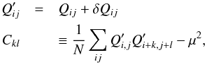 where Q and Q′ refer to the unperturbed and perturbed images respectively; μ is their (common) average; and N is the number of pixels in the sum.
We have 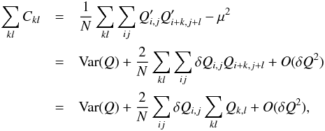 where the last transformation is only exact for unbounded sums. Since the perturbations exactly conserve charge, we have ∑ ijδQi,j ≡ 0, and hence the perturbation preserves the sum of the correlations to first order of perturbations. We note that
charge conservation is almost exact over small image patches and hence, ignoring boundary effects in the algebraic argument makes sense. This property allows us to recover the Poisson variance V(Q) by summing all correlations ∑ klCkl. It should be emphasized that, only a subset of the Ckl are summed (for instance, 81 coefficients are summed in Fig. 10) in practice, which always results in an underestimation of the Poisson variance (about 0.5% underestimation on these examples).
In Downing et al. (2006), it is also proposed to rebin the image to recover the linearity of the PTC. Rebinning still leaves some correlation between larger pixels and hence cannot exactly provide the variance of independent pixels. If one rebins an image into n times bigger pixels (in each direction), the expression for the variance of the “big” pixels divided by n2 is a linear combination of covariances, with coefficients smaller than 1, and which approaches 1 as one rebins into pixels of increasing size. For example, the covariance of nearest neighbors is multiplied by (n − 1) /n for the variance of a rebinned image (by n in both direction). Rebinning provides an easy and fair approximation of the Poisson variance but is not exact. One has to rebin by typically 10 to approach a 1% accuracy of the variance around the full well.
All Tables
Comparison of the brighter-fatter effect in the X and Y direction that are observed on CCD E2V-250, DECam and MegaCam.
Upper limit of diffusion variation for CCD E2V-250 illuminated by 550 nm spots and for DECam CCD N17 in r-band.
All Figures
|
Fig. 1 Direct shape comparison of bright and faint spots from the CCD E2V-250. The leftmost image is the average of 200 s exposures; and the middle one averages 20 s exposures; the rightmost image is the difference after proper scaling of 200 s spot image minus 20 s spot images. The broader wings and lower peak of the bright spot clearly show up. Since the images required a small alignment prior to subtraction, we have shifted both averages by half their separation, so that resampling affects both in the same way. |
| In the text | |
|
Fig. 2 Top: relative variation of spot width as a function of spot peak flux on CCD E2V-250 at two wavelengths, 550 nm (left panel) and 900 nm (right panel). Bottom left: MegaCam difference of second moments of stars to the average as a function of peak flux. Bottom right: same measurement on DECam CCD (S11). A small color correction is applied in both cases. One notes that in all cases the size increases linearly with the peak flux. |
| In the text | |
|
Fig. 3 Top: maximum (50 kADU) relative amplitude of the brighter-fatter effect in DECam. The relative slope becomes steeper when the IQ improves. Bottom: maximum amplitude of the variation of PSF shape in the various filters. The brighter-fatter effect seems achromatic, and the linear IQ increase seems fairly independant of IQ. |
| In the text | |
|
Fig. 4 a) Measured photon transfer curve of amplifiers #1 to #8 of the CCD E2V-250 expressed in ADU. b) PTCs are converted in e− using the readout gain measured as the inverse of the slope at the origin (see Sect. 4.3). Because departure from linearity of the PTCs is similar for different amplifiers this indicates that the cause of the effect is to be found in the CCD itself rather than in the electronic readout. |
| In the text | |
|
Fig. 5 CCD E2V-250: Residuals of the PTCs to the expected Poissonnian noise. The departure from linearity starts from the very beginning. |
| In the text | |
|
Fig. 6 Superposition of the evolution with flux for nearest pixel correlations (coefficients R0,1R1,1R1,0) for read out channels 1 to 8 of CCD E2V-250. The whole dynamical range shows a threshold where correlations strongly increase: first R0,1, a correlation in Y direction, and near full well, R1,0, a correlation in X direction. The diagonal correlation R1,1 does not exhibit any threashold. This is expected since neither transfer nor read out could contribute to correlate pixels in this direction. The vertical dark line indicates the early threshold of R0,1. |
| In the text | |
|
Fig. 7 2D correlation map in flatfields at a 50 ke− level for a) CCD E2V-250 (channel 4, the channel on which spots illumination presented in the first section were done); b) DECam (CCD S11); and c) MegaCam. Row and column, respectively, correspond to label X and Y. An anisotropy between the amplitudes of the R0,1 and R1,0 coefficients is observed. For distance separations larger than 1 pixel, this anisotropy tends to vanish (RX,Y ≈ RY,X for X and Y > 1). |
| In the text | |
|
Fig. 8 Variation of correlation coefficients (measured at 100 ke−) with respect to BSS measured on the CCD E2V-250. Top panel: R0,1. Middle panel: R1,0. Bottom panel: R0,2 and R2,0. The other long range correlations behave like R0,2 and R2,0: they decrease as the BSS voltage increases. |
| In the text | |
|
Fig. 9 Superposition of evolution with respect to flux of coefficients R0,1R1,1, and R1,0 on the dynamical range below the threshold, as indicated by the vertical black line of Fig. 6. On this interval, all the linearly increasing correlations that are discussed in this section shows a monotonic behavior. On this CCD E2V-250, most channels exhibit a small (≈–0.003), but significant anti-correlation pedestal in R1,0 (Y-intercept), an offset that is not seen with the others coefficients nor with the other sensors. We attribute it to the electronic chain used to collect this data, and we subtract it to the actual measurements. |
| In the text | |
|
Fig. 10 Comparison for the CCD E2V-250 between the expected Poisson noise (red dashed line) and raw PTCs that are corrected by summing covariances up to 4 pixels distance. For a 100 ke− flux level, these correlations add up to 18% of the variance. The corrected PTCs slopes coincide with Poisson law at ≈0.5%, indicating that more than 97% of the correlations are considered by the truncation at a 4 pixels distance of the integral of the correlation function. |
| In the text | |
|
Fig. 11 Electrostatic calculation of Coulombian forces generated by the electrode voltage (CV), the depletion voltage (BSS), and the electrons collected. This figure is a zoom of the last 20μm of 100μm thick simulated pixels. The black lines represent the electric field for empty pixels, and the red lines represent the electric field when the right most pixel is filled with 50 ke−. The separations between two adjacent pixels are indicated by the bold lines and are shifted to the right when adding the charges. This results in a variation of pixel effective size: the size of the filled pixel has decreased, while the size of neighbor pixel has increased (and its centroid has slightly shifted). This figure also qualitatively confirms the observation that the effect is achromatic: we see that drift trajectories are altered in the bottom ~10μm of the device only, and hence do not depend significantly on the conversion depth. |
| In the text | |
|
Fig. 12 Illumination with a spot having 100 ke− in pixel maximum and a Gaussian shape with a rms of 1.6 pixel results in boundary displacements (multiplied by a factor 5, red lines) that depend on the distribution of charges within surrounding pixels (colored circles). The displacements between the intial boundaries (black) and their final positions (red) correspond to the δX terms of our model. It shows that the central pixel effective size shrinks as illumination increases, while pixels away from spot center tend to grow. |
| In the text | |
|
Fig. 13 Correlation coefficients of the non-nearest neighbors for the CCD E2V-250 are represented as a function of their distance (black triangles) and the correlation coefficients reconstructed from a χ2 minimization (red circles) using an Exponential Integral function. This function is used to estimate the last boundaries displacement. |
| In the text | |
|
Fig. 14 Boundary displacements ( |
| In the text | |
|
Fig. 15 Top panel: IQ variation for 100 ke− (peak) spots after having redistributed the charges (on a range comparable to what was presented for DECam on Fig. 3). The accuracy of the approximation of the interpolation method (in red) is compared with the result found using the exact charge density (in blue). Bottom panel: residuals. For an IQ of 1.6 pixel, such as 550 nm spots on CCD E2V-250, the approximation introduced an underestimate below 0.1% on the size of the spot, which is less than 5% of the amplitude of the effect. |
| In the text | |
|
Fig. 16 Comparison between the broadening of spots from the redistribution and the data (CCD E2V-250, 900 nm spots). The ten low flux spots (≈13 ke−) are redistributed after increasing normalization to cover dynamical range (shaded areas). This shows the ability of our model of pixel effective size to reproduce the spot size increase observed in the brighter-fatter effect. |
| In the text | |
|
Fig. 17 Spot size along X and Y directions for 550 nm spots (top panel) and 900 nm spots (middle panel) on the CCD E2V-250. Raw spots are fitted with lines and measurements after redistribution of charges with the inverse model are shown with shaded area. Light colors correspond to dispersion coming from spot size measurements while darker colors represent the propagation of statistical 1σ uncertainties on correlations coefficients given that 50 pairs of flats were used. The five dashed lines on the lower panel indicate the redistribution prediction for the spot broadening in the Y direction when taking an increasingly large area of pixel correlations into account. It ranges from ±1 pixels distances to ±4 pixels and ±4 pixels plus the limit condition (4 + LC) established in the previous section. In the latter case, it is found that the correction restores the invariance of the PSF size with respect to increasing flux with a relative precision below 5‰ at 550 nm and 3.4‰ at 900 nm. The bottom panel represents the brighter-fatter effect as a function of the extension of the solution with the limit condition taken into account. It shows that the boundaries displacement at distance further than 4 pixels have a negligible impact on the solution. |
| In the text | |
|
Fig. 18 Measured brighter-fatter effect and simulated effect seen on DECam CCD S11 and showing the propagation of correlation coefficient uncertainties. A ±1σ rms is 0.005 pixel at 100 ke−, giving a 25% relative uncertainty, which is slightly more than the dispersion measured on this stack of 20 astronomical images. |
| In the text | |
|
Fig. 19 Comparison of measured and simulated brighter-fatter slopes for DECam r-band. There are 57 CCDs over the 62 that are presented: we reject five CCDs for which at least one of its amplifiers has a reduced χ2 for the linear fit of the correlation R1,1 that is above 3. Astronomical images are being corrected at the pixel level to take non linearities detected from looking at flatfield mean fluxes versus exposure time into account. This increases the measured slopes by about 60%. While this correction is quite important, very small changes in the way non-linearities are fitted could account for the disagreement between measurements and model. |
| In the text | |
|
Fig. 20 Average brighter-fatter slope in the X and Y direction for the MegaCam mosaic. The observations gather all the deep field (D1) r-band images of the CFHTLS (≈1.8 M stars). The redistribution prediction is based on the mean correlations of all the CCDs; this is necessary to palliate the lack of statistics given the small frame of the flatfields data set. The prediction is compatible with the observations but with a significant uncertainty. |
| In the text | |
Current usage metrics show cumulative count of Article Views (full-text article views including HTML views, PDF and ePub downloads, according to the available data) and Abstracts Views on Vision4Press platform.
Data correspond to usage on the plateform after 2015. The current usage metrics is available 48-96 hours after online publication and is updated daily on week days.
Initial download of the metrics may take a while.