| Issue |
A&A
Volume 574, February 2015
|
|
|---|---|---|
| Article Number | A126 | |
| Number of page(s) | 30 | |
| Section | Extragalactic astronomy | |
| DOI | https://doi.org/10.1051/0004-6361/201424866 | |
| Published online | 05 February 2015 | |
The Herschel Virgo Cluster Survey
XVIII. Star-forming dwarf galaxies in a cluster environment⋆
1
Centro de Astronomia e Astrofísica da Universidade de Lisboa,
OAL, Tapada da Ajuda,
1349-018
Lisbon, Portugal
e-mail: This email address is being protected from spambots. You need JavaScript enabled to view it.
2
Instituto de Astrofísica e Ciências do Espaço, Universidade de
Lisboa, OAL, Tapada da
Ajuda, 1349-018
Lisbon,
Portugal
3
Departamento de Física, Faculdade de Ciências, Universidade de
Lisboa, Edifício C8, Campo
Grande, 1749-016
Lisbon,
Portugal
4
INAF – Osservatorio Astrofisico di Arcetri,
Largo Enrico Fermi 5,
50125
Firenze,
Italy
5
Laboratoire AIM, CEA/DSM – CNRS – Université Paris Diderot,
Irfu/Service d’Astrophysique, CEA Saclay, 91191
Gif-sur-Yvette,
France
6
Sterrenkundig Observatorium, Universiteit Gent,
Krijgslaan 281, 9000
Gent,
Belgium
7
School of Physics and Astronomy, Cardiff University,
Queens Buildings, The Parade,
Cardiff
CF24 3AA,
UK
8
UK ALMA Regional Centre Node, Jodrell Bank Centre for
Astrophysics, School of Physics and Astronomy, University of Manchester,
Oxford Road, Manchester
M13 9PL,
UK
9
Center for Astrochemical Studies, Max-Planck-Institut für
extraterrestrische Physik (MPE), Giessenbachstraße, 85748
Garching,
Germany
10
Institute of Astronomy, University of Cambridge,
Madingley Road, Cambridge
CB3 0HA,
UK
11
Laboratoire d’Astrophysique de Marseille, UMR 6110
CNRS, 38 rue F.
Joliot-Curie, 13388
Marseille,
France
12
INAF – Osservatorio Astronomico di Padova,
Vicolo dell’Osservatorio 5,
35122
Padova,
Italy
13
Centre for Astrophysics and Supercomputing, Swinburne University
of Technology, Mail H30 – PO Box
218, Hawthorn,
VIC
3122,
Australia
14
Max-Planck-Institut für extraterrestrische Physik
(MPE), Postfach 1312,
Giessenbachstraße, 85748
Garching,
Germany
15
Joint ALMA Observatory/European Southern
Observatory, 3107 Alonso de Cordova,
Vitacura, Santiago,
Chile
Received: 27 August 2014
Accepted: 11 November 2014
Abstract
To assess the effects of the cluster environment on the different components of the interstellar medium, we analyse the far-infrared (FIR) and submillimetre (submm) properties of a sample of star-forming dwarf galaxies detected by the Herschel Virgo Cluster Survey (HeViCS). We determine dust masses and dust temperatures by fitting a modified black body function to the spectral energy distributions (SEDs). Stellar and gas masses, star formation rates (SFRs), and metallicities are obtained from the analysis of a set of ancillary data. Dust is detected in 49 out of a total 140 optically identified dwarfs covered by the HeViCS field; considering only dwarfs brighter than mB = 18 mag, this gives a detection rate of 43%. After evaluating different emissivity indices, we find that the FIR-submm SEDs are best-fit by β = 1.5, with a median dust temperature Td = 22.4 K. Assuming β = 1.5, 67% of the 23 galaxies detected in all five Herschel bands show emission at 500 μm in excess of the modified black-body model. The fraction of galaxies with a submillimetre excess decreases for lower values of β, while a similarly high fraction (54%) is found if a β-free SED modelling is applied. The excess is inversely correlated with SFR and stellar masses. To study the variations in the global properties of our sample that come from environmental effects, we compare the Virgo dwarfs to other Herschel surveys,such as the Key Insights into Nearby Galaxies: Far-Infrared Survey with Herschel (KINGFISH), the Dwarf Galaxy Survey (DGS), and the HeViCS Bright Galaxy Catalogue (BGC). We explore the relations between stellar mass and Hi fraction, specific star formation rate, dust fraction, gas-to-dust ratio over a wide range of stellar masses (from 107 to 1011 M⊙) for both dwarfs and spirals. Highly Hi-deficient Virgo dwarf galaxies are mostly characterised by quenched star formation activity and lower dust fractions giving hints for dust stripping in cluster dwarfs. However, to explain the large dust-to-gas mass ratios observed in these systems, we find that the fraction of dust removed has to be less than that of the Hi component. The cluster environment seems to mostly affect the gas component and star formation activity of the dwarfs. Since the Virgo star-forming dwarfs are likely to be crossing the cluster for the first time, a longer timescale might be necessary to strip the more centrally concentrated dust distribution.
Key words: galaxies: dwarf / galaxies: clusters: general / galaxies: ISM / dust, extinction / infrared: ISM
Appendices are available in electronic form at http://www.aanda.org
© ESO, 2015
1. Introduction
Dust, gas, and star formation activity are tightly linked in galaxies, implying that
detailed investigation of these components and of their mutual relation is fundamental for
our understanding of galaxy evolution. It is known that one of the main roles of dust in the
star formation cycle of galaxies is the formation of molecular hydrogen (Gould & Salpeter 1963; Hollenbach & Salpeter 1971). As galaxies form stars, their
interstellar medium (ISM) becomes enriched in dust, and galaxies with a higher star
formation rate are found to host a more massive dust component (da Cunha et al. 2010). Dust is observed to be well mixed with gas (Bohlin et al. 1978; Boulanger et al. 1996), and dust formation models show that the dust-to-gas
ratios,  ,
should be tied to the oxygen abundance of a galaxy (Dwek
1998; Sandstrom et al. 2013).
,
should be tied to the oxygen abundance of a galaxy (Dwek
1998; Sandstrom et al. 2013).
It is still not clear, however, how dust properties and their link with gas and star formation activity vary when we consider galaxies in a dense cluster, where external perturbations can affect the ISM content and star formation activity. Indeed the evolution of galaxies in clusters is driven by interactions between their ISM and the surrounding environment: ram pressure stripping (Gunn & Gott 1972; Quilis et al. 2000; Tonnesen et al. 2007), harassment (Moore et al. 1996, 1998), tidal interactions (Brosch et al. 2004), and strangulation (Larson et al. 1980; Kawata & Mulchaey 2008) are among the processes that can be responsible for removing the ISM and quenching star formation. Studies of nearby rich clusters have shown that ram pressure stripping can be the dominant transformation process of star-forming galaxies into quiescent systems (Crowl et al. 2005; Boselli & Gavazzi 2006; Gavazzi et al. 2013a).
It is well established that late-type galaxies in dense environments tend to have less Hi than their field counterparts and that there is an anticorrelation between the Hi deficiency and the distance to the cluster centre (Giovanardi et al. 1983; Haynes & Giovanelli 1984; Chung et al. 2009). On the other hand, it is debated whether this is not also true for the molecular gas component that is usually more centrally concentrated (Fumagalli et al. 2009; Pappalardo et al. 2012; Boselli et al. 2014b) and for the dust that is supposed to be more closely linked to the molecular than to the atomic gas phase. Before the launch of the Herschel Space Observatory (Pilbratt et al. 2010), the influence of the environment on the removal of dust in Hi-deficient spirals has been addressed in studies using observations with both the Infrared Astronomical Satellite (IRAS, Doyon & Joseph 1989) and the Infrared Space Observatory (ISO, Boselli & Gavazzi 2006). However, the small number of studied objects and the lack of an unperturbed reference sample prevented drawing conclusions on dust stripping in high-density environments. Only recent observations with Herschel were able to show that dust can be stripped from Virgo cluster galaxies (Cortese et al. 2010; Gomez et al. 2010), providing conclusive evidence that it is significantly reduced in the discs of very Hi deficient cluster spirals (Cortese et al. 2012; Corbelli et al. 2012).
The Virgo cluster, at a distance of approximately 17 Mpc (Gavazzi et al. 1999; Mei et al. 2007) and comprising ~1300 confirmed members (Binggeli et al. 1985), is indeed the nearest example of a high-density environment. It contains about two hundred star-forming dwarf (SFD) galaxies – i.e. classified as Sm, Im, and blue compact dwarfs (BCDs) according to the Virgo Cluster Catalogue (Binggeli et al. 1985) and GOLDMine (Gavazzi et al. 2003, 2014). Because of their lower gravitational potentials and less dense ambient ISM (Bolatto et al. 2008), dwarfs are more sensitive to their surroundings than more massive galaxies, which makes them excellent targets for investigating the environmental effects on a weakly bound ISM (Boselli et al. 2008).
Through the Herschel Virgo Cluster Survey (HeViCS; Davies et al. 2010, 2012), a Herschel Open Time Key Project that covers ~80 square degrees of the Virgo cluster from 100 μm to 500 μm, we present an analysis of the far-infrared (FIR) and submillimetre (submm) observations of a sample of SFDs in this cluster. We discuss their FIR properties, the relation between dust and other global galaxy parameters (i.e. stellar mass, star formation rate, and gas content), and analyse the effects of the environment on the dust component.
Previous Virgo surveys with IRAS (Neugebauer et al. 1984) and ISO (Kessler et al. 1996) also targeted the SFD population. About one third of the cluster BCDs were detected at 60 and 100 μm; their dust content, compared to their stellar and gas masses, is only a factor 2 to 3 smaller than normal spiral galaxies. The warm IRAS colours also suggested that the FIR luminosity was dominated by the emission from star-forming regions (Hoffman et al. 1989). Popescu et al. (2002) and Tuffs et al. (2002) analysed a small sample of late-type Virgo galaxies including irregulars and BCDs with ISOPHOT, finding very cold dust temperatures (a median value of 15.9 K), and extended dust distributions similar to the size of the Hi discs. However, given the small number of objects investigated, the lack of coverage beyond 200 μm where cold dust emission is predominant, and the large beam size of the ISOPHOT instrument at 170 μm (FWHM ~ 1′), further investigations over a larger sample and a wider spectral coverage is required to better assess the dust content of Virgo SFDs.
The paper is organised as follows. In Sect. 2 we briefly describe the HeViCS survey observations and data reduction, and in Sect. 3 the sample selection and the photometry. In Sect. 4 we present the samples that will be used as a comparison throughout the paper: 1) the Key Insights into Nearby Galaxies: Far-Infrared Survey with Herschel (KINGFISH, Kennicutt et al. 2011; Dale et al. 2012); 2) the Dwarf Galaxy Survey (DGS; Madden et al. 2013; Rémy-Ruyer et al. 2013), both targeting systems in lower density environments; 3) the brightest galaxies in the HeViCS survey (Davies et al. 2012). We list the ancillary data available in the literature for all these surveys in Sect. 5. In Sect. 6 we analyse the FIR-submm SEDs of the detected Virgo SFDs, and infer dust temperatures and masses, using different values for the emissivity index β. The properties of FIR-detected and FIR-undetected Virgo SFDs are compared in Sect. 7. The presence of a submm excess emission at 500 μm is discussed in Sect. 8. The global properties of the ISM and dust-scaling relations are investigated in Sect. 9, comparing Virgo SFDs to the other Herschel surveys. Finally, in Sect. 10 we summarise our conclusions.
2. Herschel observations
The HeViCS survey consists of four fields with a size of ~4° × 4° each, covering the main structures of the cluster: the M87 and M49 subgroups, the W, W′, and M clouds (Binggeli et al. 1987; Mei et al. 2007). Herschel Photodetecting Array Camera and Spectrometer (PACS; Poglitsch et al. 2010) and Spectral and Photometric Imaging Receiver (SPIRE; Griffin et al. 2010) observations of Virgo were taken between December 2009 and June 2011. A more detailed description of the observing strategy and data reduction process is given in the HeViCS overview and catalogue papers (Davies et al. 2012; Auld et al. 2013, hereafter A13), and a brief summary of the main steps followed are given below.
Herschel observations were carried out using the SPIRE/PACS parallel scan-map mode with a fast scan speed of 60′′/s over two orthogonal crossed-linked scan directions. A total of 8 scans was then obtained for each field, with overlapping regions between the four tiles being covered by 16 scans.
Regarding the PACS data release, we used a more recent version compared to that described in A13. Data at 100 and 160 μm were reduced within the Herschel Interactive Processing Environment (version 11.0; Ott 2010), and maps were created with the Scanamorphos task (version 23; Roussel 2013) with a pixel size of 2′′ and 3′′, respectively. The angular resolution for PACS in fast scan parallel mode is 9.̋4 and 13.̋4, at 100, and 160 μm, respectively. Maps attain noise levels of 1.9 and 1.2 mJy pixel-1 which decrease to 1.3 and 0.8 mJy pixel-1 in the regions covered by 16 scans. A calibration uncertainty of 5% is assumed for both 100 and 160 μm channels (Balog et al. 2013).
SPIRE data reduction was carried out up to Level 1 adapting the standard pipeline (POF5 pipeline.py, dated 8 Jun. 2010) provided by the SPIRE Instrument Control Service (Griffin et al. 2010; Dowell et al. 2010), while temperature drift correction and residual baseline subtraction were performed using the BriGAdE method (Smith 2012). Final maps were created with the naive mapper provided by the standard pipeline (naiveScanmapper task in HIPE v9.0.0), with pixel sizes of 6′′, 8′′, and 12′′ at 250, 350, and 500 μm, respectively. The global noise level in the SPIRE images is 4.9, 4.9, and 5.7 mJy beam-1 (at 250, 350, 500 μm; A13). The calibration uncertainty for SPIRE flux densities is 6% for each band1, and the beam size full width at half maximum (FWHM) in the three channels is 17.̋6, 23.̋9, and 35.̋2.
Given the new analysis of the SPIRE beam profile we adopt the revised beam areas of 465.4, 822.6, 1768.7 square arcseconds (SPIRE Handbook, version 2.5)2 to derive flux densities at SPIRE wavelengths. We applied the updated KPtoE conversion factors to optimise the data for extended source photometry, i.e. 91.289, 51.799, 24.039 MJy sr-1 (Jy beam-1)-1, as indicated in the SPIRE handbook, and the latest calibration correction factors (1.0253 ± 0.0012, 1.0250 ± 0.0045, and 1.0125 ± 0.006 at 250, 350, and 500 μm, respectively).
3. Virgo star-forming dwarfs: sample selection and photometry
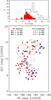 |
Fig. 1 Upper panel: distribution of apparent B magnitudes of the Virgo Sm, Im, and BCD galaxies in the four HeViCS fields. The red filled histogram shows the galaxies detected by Herschel. The dotted line corresponds to the completeness limit of the VCC catalogue. Lower panel: spatial distribution of the Sm, Im, and BCD galaxies in the four HeViCS fields. Grey circles show the main substructures within the cluster. Filled red, pink, and purple dots indicate FIR detections in at least two Herschel bands at distances of 17, 23, and 32 Mpc, respectively, that will be analysed in this work. Triangles with the same colour codes correspond to FIR non-detections at the three distance ranges. |
3.1. Sample selection
The HeViCS fields contain 140 galaxies classified in the Virgo Cluster Catalogue (VCC; Binggeli et al. 1985) and in the GOLDMine database (Gavazzi et al. 2003, 2014) as Sm, Im, BCD/dIrr3 with radial velocity V< 3000 km s-1. The galaxies span a varied range of B magnitudes and radial velocities. B magnitudes of the selected objects are between 12 and 21 mag (upper panel of Fig. 1), the radial velocity distribution of the galaxies extends from –200 km s-1 to 2700 km s-1. Virgo SFDs are spread along the different substructures within the cluster: a) the main body of the cluster centred on the cD galaxy M87 (cluster A, V ~ 1100 km s-1); b) the smaller subcluster centred on the elliptical galaxy M49 roughly at the same distance as M87 (cluster B, V ~ 1000 km s-1); c) the so-called low-velocity cloud (LVC), a subgroup of galaxies at V~< 0 km s-1 superposed to the M87 region which is thought to be infalling towards the cluster core from behind (Hoffman et al. 1989); d) the Virgo Southern extension (S), a filamentary structure that extends to the south of the cluster; e) the W and M clouds, to the southwest and to the northwest of the cluster core respectively, at roughly twice the distance of M87 (V ~ 2200 km s-1; Ftaclas et al. 1984; Binggeli et al. 1987); the W′ cloud, a substructure which connects the W cloud to the M49 subgroup. Following GOLDMine we assume three main values for the distances to the objects of the sample: 17 Mpc, whether they belong to the M87 and M49 subclusters, the LVC, and Virgo Southern extension; 23 Mpc for the W′ cloud and the substructure rich in late-type galaxies between cluster A and B; 32 Mpc for galaxies in the M and W clouds. We note that distance assignment to individual objects of the Virgo cluster can be highly uncertain, and according to Gavazzi et al. (2005) errors on distances to Virgo members can be as high as 30%.
The distribution of SFD galaxies within the cluster and the substructures at larger distances is shown in Fig. 1. Galaxies in each subgroup are probably at different stages of interaction with the surrounding environment, and it is likely that a fraction of the SFDs at d ~ 17 Mpc are entering the cluster for the first time (Binggeli et al. 1993; Gavazzi et al. 2002; Hoffman et al. 2003).
It is important to note that the W′, W, and M structures are outside the virial radius of the cluster and represent an intermediate density environment between the cluster and the field. Significant Hi deficiencies were identified in galaxies even at large distances from the Virgo core, well beyond the extension of the hot X-ray intracluster medium mainly in correspondence with the W′ and W clouds (Solanes et al. 2002). However, in a recent analysis of the Hi content of Virgo late-type galaxies, Gavazzi et al. (2013a) reported that the W and M cloud population do not appear to have a large atomic hydrogen deficit.
3.2. Herschel detections: SPIRE/PACS photometry
Within the initial sample of 140 SFDs, 57 have a FIR-submm detection in the HeViCS catalogue (A13), with at least one detection in one Herschel band with a signal-to-noise ratio S/N> 3. Because we used an updated release of the PACS maps compared to that in A13, we remeasured the photometry at PACS wavelengths. We also recalculated the photometry at 250, 350, and 500 μm in order to have an homogeneous set of measurements obtained with the same method, despite having used the same data release as A13.
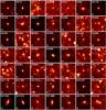 |
Fig. 2 250 μm image stamps of the sample of star-forming dwarf galaxies detected by HeViCS. The field size is 180′′. The SPIRE beam size at 250 μm is shown at the lower-left corner of each image stamp. |
Flux densities of extended sources were measured through elliptical apertures defined on the basis of the isophotal semi-major (a25) and semi-minor axis (b25) at the 25th B-magnitude arcsec-2, which were taken from the GOLDMine database. Apertures were chosen to be ~1.5 times the optical radii. For a few galaxies (VCC1, VCC24, VCC322, VCC1021, VCC1179, VCC1200, VCC1273), smaller apertures were adopted (~1.0 times the optical radii). For the most compact dwarfs, i.e. with a25 smaller or comparable to the Herschel resolution at 500 μm, we used circular apertures with 30′′ radii (VCC22, VCC223, VC281, VCC334, VCC367, VCC1141, VCC1437). These same apertures were applied to derive flux densities at all wavelengths. However, to measure PACS 100 μm photometry we tended to use smaller apertures (by a factor ~0.65) because of the reduced extent of the dust emission at this wavelength compared to the stellar disc (see also Table C.1). This choice allowed us to prevent an artificial increase of the error associated with our measurement. The background was measured following the approach of A13, i.e. the estimate was achieved with a 2D polynomial fit over an area of 180′′ around the aperture defined to extract the galaxy emission, after having masked the galaxy. Following A13, a fifth order polynomial was used to determine the background in SPIRE images, while a second order polynomial was sufficient for PACS data. To reduce the contribution of possible contaminating sources a 95% flux clip was applied before estimating the background. As a comparison we also estimated the background in fixed annuli with a 60′′ width, and found that on average we obtained a better curve of growth convergence with the 2D polynomial fit. The difference in the final flux densities between the two methods is less than 10–15%, which is close to the relative error at all wavelengths.
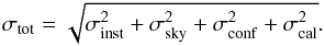
Uncertainties were calculated following Ciesla et al.
(2012), adding in quadrature the instrumental error, σinst, the sky
background error, σsky, the confusion noise due to the
presence of faint background sources, σconf (calculated only for SPIRE images;
Nguyen et al. 2010), and the error on the
calibration, σcal, assumed to be 5% and 6% for PACS and
SPIRE channels, respectively (see Sect. 2):
 (1)The instrumental error, σinst, depends
on the number of scans crossing a pixel, and it was obtained by summing in quadrature the
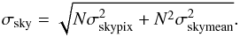
values on the error map provided by the pipeline within the chosen aperture. The sky
background error, σsky, results from the combination of
the uncorrelated uncertainty on the mean value of the sky (σskypix i.e.,
the pixel-to-pixel variation in the region where we derived the sky background), and the
correlated noise (σskymean) due to large scale structures
present in the image such as the Galactic cirrus (Ciesla
et al. 2012; Roussel 2013; Cortese et al. 2014). To estimate σskymean we
defined 24 apertures around each galaxy with the same number of pixels N used to measure the
galaxy flux density, and we calculated the standard deviation of the mean value of the
sky. The sky background uncertainty was then given by
(1)The instrumental error, σinst, depends
on the number of scans crossing a pixel, and it was obtained by summing in quadrature the
values on the error map provided by the pipeline within the chosen aperture. The sky
background error, σsky, results from the combination of
the uncorrelated uncertainty on the mean value of the sky (σskypix i.e.,
the pixel-to-pixel variation in the region where we derived the sky background), and the
correlated noise (σskymean) due to large scale structures
present in the image such as the Galactic cirrus (Ciesla
et al. 2012; Roussel 2013; Cortese et al. 2014). To estimate σskymean we
defined 24 apertures around each galaxy with the same number of pixels N used to measure the
galaxy flux density, and we calculated the standard deviation of the mean value of the
sky. The sky background uncertainty was then given by
 (2)The confusion noise σconf was
determined using Eq. (3) of Ciesla et al. (2012)
and the estimates given by Nguyen et al. (2010).
(2)The confusion noise σconf was
determined using Eq. (3) of Ciesla et al. (2012)
and the estimates given by Nguyen et al. (2010).
For some of the dwarfs the extent of the emission at 500 μm is comparable to the FWHM of SPIRE and appear as marginally resolved. The flux density of point-like sources can be extracted directly from the timeline data using a PSF fitting method (Bendo et al. 2013). This method provides a more reliable estimate than the aperture photometry technique of unresolved sources (Pearson et al. 2013), especially in the case of faint detections (~20–30 mJy). To check whether some of the dwarfs of our sample could be treated as point-like sources we cross-correlated our list of detected galaxies with the HeViCS point-source catalogue (Pappalardo et al. 2015), finding 21 matches. For these objects flux densities were estimated with a timeline-based point source fitter that fits a Gaussian function to the timeline data. More detail about the catalogue and the source extraction technique can be found in Pappalardo et al. (2015). Errors on the flux densities of point sources were determined directly from the timeline fitting technique.
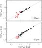 |
Fig. 3 Comparison between PACS 100 and 160 μm flux densities derived in this work (FTW) and in A13 (FA13). The one-to-one relation is given by the dotted line. At S/N> 5 there is good agreement between our values and A13 at both wavelengths (black dots). Red dots show lower S/N detections (3 <S/N< 5). |
We decided to include in our final sample only galaxies with at least a detection in two bands with S/N> 3, with a total of 49 objects satisfying this criterion. Compared to the A13 catalogue we do not take into account the following galaxies: VCC309, VCC331, VCC410, VCC793, VCC890, VCC1654, VCC1750, because they have a detection in only one band. We also rejected VCC83 and VCC512 because of possible contamination from background galaxies which may affect the correct assessment of the FIR-submm flux densities. Finally we added to the list of detections VCC367 which appears to be missing from the A13 catalogue. Herschel/SPIRE cut-out images of the final sample at 250 μm are shown in Fig. 2.
Comparison with PACS photometry derived in A13 (Fig. 3) shows a good agreement between our and previous measurements at least for sources with S/N> 5 (black dots). At lower S/N, and especially at 100 μm, there is a larger discrepancy. This could be due to both the better performances of Scanamorphos compared to HIPE at preserving low level flux densities, and to our choice of using apertures smaller than 1.4 times the optical extent of the galaxy to reduce the contribution of the background to the measured flux densities of low S/N 100 μm detections.
3.3. Stacking of non-detections
The mean FIR emission of the undetected galaxy population can be explored to deeper levels by stacking 250 μm images of the dwarfs at their optical positions. Among the FIR non-detections we selected galaxies with mB< 18 mag, according to the completeness limit of the VCC catalogue. We excluded VCC169 and VCC217 because they were too close to the edges of the HeViCS map, and four objects showing nearby background sources which could affect the result of the stacking process (VCC83, VCC168, VCC468, and VCC512). The final list of undetected galaxies to stack includes 64 dwarfs. For each sub-image with a size of 50 × 50 pixels we computed the root mean square (rms) with iterative sigma clipping, and masked all sources above 5σ in the region outside a circular aperture of 5 pixel radius (30′′) around the position of the galaxy. Then we derived the mean of each pixel weighted by the square of the inverse of the background rms of the corresponding sub-image. The rms of the stacked image, shown in Fig. 4 is 0.85 mJy/beam, about 8 times lower than the mean rms of the 64 input sub-images (6.7 mJy/beam). This offers a significant improvement over the original data set, giving evidence for a 3.5σ detection with a flux density of 4.5 mJy within a circular aperture of 4 pixel radius. For comparison we repeated the same procedure median combining the images without masking the brighter sources scattered around the sub-images, and obtained a slightly higher rms (1.0 mJy/beam) with a final S/N ratio of 3.1.
We estimate the average dust mass of undetected galaxies in Sect. 6.3 and we discuss their properties in Sect. 7.
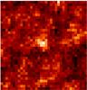 |
Fig. 4 Mean stacked image at 250 μm of 64 dwarf galaxies with mB< 18 undetected by HeViCS. The image has a rms of 0.85 mJy/beam. The 3.5σ detection at the centre has a flux density of ~4 mJy. |
4. Selection of comparison samples
To assess the effects of the cluster environment on the dust content of the dwarf galaxies in Virgo we use, as a comparison sample, dwarfs extracted from other Herschel surveys targeting lower density environments.
The Dwarf Galaxy Survey (DGS, Madden et al. 2013) is a photometric and spectroscopic survey of 50 dwarf galaxies, which aims at studying the gas and dust properties in low-metallicity systems. Among these galaxies we selected a subset of objects which have been detected by Herschel in at least three bands (100, 160, and 250 μm), so that we can determine dust temperatures and masses in the same way as we have done for the Virgo galaxies (see Sect. 6.3). Haro11 was excluded from the final list because its properties are remarkably different from our sample of Virgo dwarfs, being a merger with a SFR of tens of solar masses per year. Therefore the final subset of selected DGS galaxies includes 27 objects. Herschel photometry for this sample was taken from Rémy-Ruyer et al. (2013). To take into account the updated SPIRE calibration we multiplied their flux densities for the correction factors given in Sect. 2.
KINGFISH is an imaging and spectroscopic survey of 61 nearby (d< 30 Mpc) galaxies, chosen to cover a wide range of morphological types and ISM properties (Kennicutt et al. 2011). Among the 61 KINGFISH objects, there are 12 Irregular/Magellanic-type (Im/Sm) galaxies, and 39 spirals ranging from early to late types, that we will use throughout the rest of this work. We used flux densities given by Dale et al. (2012), corrected for the revised SPIRE beam areas and calibration, and we applied the updated KPtoE conversion factors as we did for the HeViCS data (Sect. 2).
Finally, to compare the properties of low-mass systems to the more massive galaxies within Virgo we include to our list of comparison samples 68 spiral galaxies (from Sa to Sd) from the HeViCS Bright Galaxy Catalogue (BGC, Davies et al. 2012). FIR-submm photometry was taken from A13 and corrected for the updated SPIRE beam sizes and calibration (see Sect. 2).
5. Ancillary data and analysis
We have assembled several sets of additional data in order to derive other properties of the Virgo SFDs and the comparison samples. These include stellar masses, atomic gas masses, star formation rates, and gas metallicities which will be incorporated in the subsequent analysis together with dust masses to better assess the effect of environment.
5.1. Stellar masses
5.1.1. Virgo SFDs
Stellar masses were calculated following the approach of Wen et al. (2013, hereafter W13) which is based on 3.4 μm photometry from the Wide-field Infrared Survey Explorer (WISE) all-sky catalogue (Wright et al. 2010)4. WISE has mapped the full sky in four bands centred at 3.4, 4.6, 12, and 22 μm (W1,W2,W3,W4), achieving 5σ point-source sensitivities of 0.08, 0.11, 1, and 6 mJy, respectively.
We performed aperture photometry on Band 1 WISE Atlas Images with SEXTRACTOR using the
prescription given by the WISE team5, applied
aperture and colour corrections as indicated in the WISE Explanatory Supplement6. Because of the potential importance of nebular
continuum and line emission in the near-infrared wave bands (e.g., Smith & Hancock 2009) we calculated and subtracted the expected
nebular contribution in the WISE band 1 according to Hunt et al. (2012) to obtain a star-only flux. Nonetheless, because of the
relatively low star-formation rates (SFRs) for the HeViCS dwarfs (see Sect. 5.3), the nebular contribution to W1 for these
galaxies is low, ~1% on
average. Stellar masses were estimated from the relation for star forming galaxies
provided in W13, ![Mathematical equation: \begin{eqnarray} \label{eq:Wen13} \log ( M_{\star}/ \tmsun ) = a + b \, \log [ \nu L_{\nu} (3.4~\mu{\rm m})/ \tlsun ] \end{eqnarray}](/articles/aa/full_html/2015/02/aa24866-14/aa24866-14-eq54.png) (3)where the a and b coefficients are given
in Table 1.
(3)where the a and b coefficients are given
in Table 1.
The errors include the uncertainties in the photometric errors and in the coefficients of the Wen et al. (2013) relation. Because of the large uncertainties in the distance to the Virgo galaxies, they are not included in the error calculation of stellar masses and of other parameters derived in this section.
We found that the approach of W13 gives stellar masses to within 10–20% of those derived with the method of Lee et al. (2006) which relies on a variable mass-to-light ratio. In Fig. A.1, we show that our stellar masses are also in good agreement with those provided by GOLDMine, which are derived from the i magnitude and (g − i)0 colour, and calibrated on the MPA-JHU sample (Gavazzi et al. 2013a), similarly to that done in W13. The residual distribution between the two estimates is displayed in the bottom panel (blue histogram), with the result of the gaussian fitting which peaks at 0.05 dex and it has a dispersion of 0.08 dex. Virgo dwarf stellar masses are listed in Table 2.
Stellar masses, Hi masses, dust masses, star formation rates, metallicities, Hi deficiency, and adopted distances of star-forming dwarf galaxies detected by HeViCS.
5.1.2. Comparison samples
To avoid systematics due to the choice of different stellar mass estimates we derived M⋆ for the comparison samples with the same method adopted for the Virgo SFDs. We chose not to derive the stellar masses with methods using optical photometry such as i-band luminosity and the (g − i) colour-dependent stellar mass-to-light ratio relation (Zibetti et al. 2009; Gavazzi et al. 2013a), because most of the DGS galaxies do not have optical photometry measurements in the literature, and only 24 KINGFISH galaxies are in the area covered by the SDSS. Therefore this would have inevitably created a systematic offset between the stellar masses of the DGS/KINGFISH and those of the other samples.
Regarding the DGS and HeViCS BGC galaxies we measured WISE W1 photometry from the WISE Atlas Images as explained in the previous section, we subtracted the expected nebular contribution to the 3.4 μm emission, and then applied Eq. (3) to derive M⋆.
The KINGFISH galaxies have IRAC 3.6 μm flux measurements in the literature. In this case we derived a conversion factor between IRAC 3.6 μm and WISE W1 flux densities and then we calculated stellar masses with Eq. (3). To derive the conversion factor we used the atlas of 129 spectral energy distributions for nearby galaxies (Brown et al. 2014), which includes measurements from both Spitzer and WISE. The atlas contain 23 spirals and 1 Sm galaxy from the KINGFISH sample; for these objects we found that the mean ratio between the two bands is F3.4/F3.6 = 1.020 ± 0.035. We applied this conversion factor to the IRAC fluxes, subtracted the expected nebular contribution, and estimated stellar masses with Eq. (3). Comparison with stellar mass estimates obtained with different methods for these three samples is discussed in Appendix A. Stellar masses of the DGS, KINGFISH, and HeViCS BGC galaxies are listed in Tables C.2–C.5.
Although it is often assumed that the 3.4/3.6 μm band is dominated by starlight we cannot rule out that a source of possible contamination to this emission could be provided by polycyclic aromatic hydrocarbons (PAH) and hot dust (Mentuch et al. 2010; Meidt et al. 2014). The issue of this possible contamination is not discussed or taken into account in Wen et al. (2013). Analysis in a small sample of disc galaxies in the Spitzer Survey of Stellar Structure in Galaxies show that hot dust and PAH can contribute between 5% and 13% of the total integrated light at 3.6 μm (Meidt et al. 2014). In a sample of local dwarf galaxies, comparison with stellar population synthesis models shows that starlight alone can account, within the uncertainties, for the 3.6 μm emission (Smith & Hancock 2009). Comparison to Gavazzi et al. (2013a) stellar mass estimates for Virgo galaxies (see also Appendix A) suggests that the possible contamination of hot dust will not significantly influence the results discussed in the rest of this work.
5.2. H I masses
5.2.1. Virgo SFDs
The atomic hydrogen (Hi) content of Virgo dwarf galaxies was derived from the Arecibo Legacy Fast ALFA (ALFALFA) blind Hi survey (Giovanelli et al. 2005). The latest catalogue release, the α.40 catalogue (Haynes et al. 2011), covers the cluster at declinations 4°<δ< 16°, almost the whole extent of the HeViCS fields. With a mean rms of 2 mJy/beam, the survey detection limit for a dwarf galaxy with S/N = 6.5 and a typical Hi line width of 40 km s-1 at a distance of 17 Mpc, is MHi ≈ 107.5 M⊙. For those galaxies not included in the ALFALFA catalogue, Hi mass measurements were obtained from the literature: VCC1 (Gavazzi et al. 2005); VCC286, VCC741 (Hoffman et al. 1987); VCC135 (Springob et al. 2005). Only five galaxies have not been detected at 21 cm (see Table 2).
Following Haynes & Giovanelli (1984) and
Gavazzi et al. (2013b), we estimated the
Hi deficiency parameter defined as the logarithmic difference between the
Hi mass of a reference sample of isolated galaxies for a given morphological
type and the observed Hi mass: Def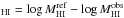 . The reference Hi mass is
derived as
. The reference Hi mass is
derived as 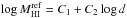 , where d is the galaxy linear
diameter in kpc at the 25th mag arcsec-2B-band isophote, and the C1 (7.51) and
C2 (0.68) coefficients have been
rederived by Gavazzi et al. (2013b) for all
late-type galaxies (independently of the Hubble type) using a sample of isolated objects
from the ALFALFA survey. A threshold of DefHI = 0.5 is adopted to distinguish
Hi-deficient from Hi-normal systems, corresponding to galaxies with at
least 70% less atomic hydrogen than expected for isolated objects of the same optical
size and morphology. Galaxies with DefHI> 0.9 are considered highly Hi-deficient
(Gavazzi et al. 2013b). Hi masses and
Hi-deficiency of the Virgo dwarfs are given in Table 2.
, where d is the galaxy linear
diameter in kpc at the 25th mag arcsec-2B-band isophote, and the C1 (7.51) and
C2 (0.68) coefficients have been
rederived by Gavazzi et al. (2013b) for all
late-type galaxies (independently of the Hubble type) using a sample of isolated objects
from the ALFALFA survey. A threshold of DefHI = 0.5 is adopted to distinguish
Hi-deficient from Hi-normal systems, corresponding to galaxies with at
least 70% less atomic hydrogen than expected for isolated objects of the same optical
size and morphology. Galaxies with DefHI> 0.9 are considered highly Hi-deficient
(Gavazzi et al. 2013b). Hi masses and
Hi-deficiency of the Virgo dwarfs are given in Table 2.
5.2.2. Comparison samples
Hi masses for the DGS galaxies were obtained from Rémy-Ruyer et al. (2014). Only four galaxies do not have a 21 cm
detection (see Table C.2). Sixteen out of 27
galaxies have a CO detection in the literature, and H2 masses have been calculated
by Rémy-Ruyer et al. (2014) using the Galactic
CO-to-H2
conversion factor,  cm-2/K km s-1 (Ackermann et al. 2011) and a metallicity dependent XCO scaling
with (O/H)-2
(Schruba et al. 2012).
cm-2/K km s-1 (Ackermann et al. 2011) and a metallicity dependent XCO scaling
with (O/H)-2
(Schruba et al. 2012).
Atomic hydrogen masses for the KINGFISH galaxies were also taken from Rémy-Ruyer et al. (2014) where they combined literature measurements from Draine et al. (2007) and Galametz et al. (2011). CO observations are available in the literature for 33 out of 51 galaxies and they have been assembled by Rémy-Ruyer et al. (2014). H2 masses were derived using two XCO factors similarly to the DGS sample. KINGFISH gas masses are displayed in Table C.3 and C.4.
Hi masses for the HeViCS BGC sample were obtained from the α.40 catalogue and the
GOLDMine database. Only four galaxies have not been detected at 21 cm: VCC341, VCC362,
VCC1190, VCC1552 (see Table C.5). For a subset
of HeViCS BGC galaxies, H2 masses are available from the Herschel
Reference Survey (HRS; Boselli et al.
2014a), and are also listed in Table C.5, calculated for both a Galactic CO-to-H2 conversion factor and a
H-band
luminosity dependent conversion factor  (Boselli
et al. 2002).
(Boselli
et al. 2002).
Figure 5 displays the Hi fraction fHI = MHI/M⋆ against the stellar mass for Virgo galaxies and the comparison samples. The Hi content of the Virgo dwarfs, as given by the Hi deficiency parameter, is highlighted by the different shapes of the circles and shades of blue: galaxies with DefHI< 0.5 have a normal Hi content (filled dots), galaxies with 0.5 ≤ DefHI< 0.9 are Hi-deficient (rings), and those with DefHI> 0.9 (ringed dots) are extremely poor in atomic hydrogen. The Hi content of DGS, KINGFISH spirals (from Sa to Sd types), KINGFISH dwarfs (objects later than Sd), and the HeViCS BGC is also shown. Gas-scaling relations of the Hα3 sample from Gavazzi et al. (2013b) are overlaid for comparison for two classes of Hi-deficiency: normal (dash-dotted line), and highly deficient systems (dotted line).
The Hi fraction decreases by approximately 4 orders of magnitude with stellar mass, from log (M⋆/ M⊙) ~7 to 11. As expected, more massive galaxies are characterised by lower gas fractions, while low-mass galaxies retain larger quantities of Hi compared to their stellar masses (Cortese et al. 2011; Huang et al. 2012; Gavazzi et al. 2013a).
Most of the Virgo dwarf galaxies with a normal atomic hydrogen content (DefHI< 0.5) show similar gas fractions to the KINGFISH and DGS dwarfs with comparable stellar masses. Among the Hi-normal Virgo SFDs, about a third fall in the region of higher Hi-deficiency defined by the gas scaling relations of Gavazzi et al. (2013b), and they do show gas fractions similar to dwarfs with 0.5 ≤ DefHI< 0.9. It is possible the DefHI is not well assessed for this subset. Approximately 20% of Virgo SFDs show a large gas deficit relative to other dwarfs, as Fig. 5 illustrates, giving a clear signature of the interaction occurring between these systems and the surrounding environment. The figure also shows the well-known decrease in the Hi fraction of Virgo late-type spiral galaxies compared to galaxies with similar stellar mass and morphological type but evolving in less dense environments such as KINGFISH objects (Cortese et al. 2011).
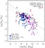 |
Fig. 5 Hi gas fraction (MHI/M⋆) as a function of stellar mass. Blue symbols correspond to the Virgo SFDs, with the different shapes indicating the atomic hydrogen content of the galaxies as given by the Hi deficiency parameter: Hi-normal (filled dots), Hi-deficient (rings), highly Hi-deficient (ringed dots). Red-purple triangles represent the DGS sample, grey squares show the spiral and dwarf galaxies of the KINGFISH sample, and purple diamonds correspond to the HeViCS BGC. Hi-deficient HeViCS BGC galaxies (DefHI ≥ 0.5) are indicated by a diamond with a cross. Gas-scaling relations from Gavazzi et al. (2013b) are overlaid for normal (dash-dotted line), and highly deficient (dotted line) galaxies. |
5.3. Star formation rates
5.3.1. Virgo SFDs
We estimated the global star-formation rate starting from Hα photometry which was obtained from the GOLDMine data base. Hα fluxes were corrected for Galactic extinction with the Schlafly & Finkbeiner (2011) extinction curve (RV = 3.1) using A(Hα) = 0.81AV. Correction for [NII] deblending was obtained calculating the [NII]λ6584/Hα ratio with line fluxes extracted from the SDSS MPA-JHU DR7 release7. A ratio of [NII]λ6548/[NII]λ6584 = 0.34 was assumed to take into account the contribution of both lines to the Hα flux (Gavazzi et al. 2012). When [NII]λ6584 line flux was not available we derived the ([NII]/Hα) ratio using the relation calibrated on the absolute i-band magnitude ([NII]/Hα) = −0.0854 × Mi −1.326 (Gavazzi et al. 2012).
To account for both unobscured and obscured star formation we followed two procedures.
First, we searched for mid-IR emission using the WISE All-Sky Survey at 22
μm, and
found 30 dwarfs with a mid-IR counterpart. For these galaxies we performed aperture
photometry on the 22 μm WISE Atlas Images with SEXTRACTOR in the same
way as described in Sect. 5.1, applied aperture and
colour corrections, and an additional correction factor of 0.92 as recommended in Jarrett et al. (2013)8. Then we used the relation of Wen et al.
(2014) to derive the SFR9: ![Mathematical equation: \begin{eqnarray} \label{eq:Wen14SFR} \log\,({\it SFR}) \, \left[M_{\odot} \, \text{yr}^{-1}\right] \!=\! \log \left[L_{{\rm H}\alpha} + 0.034 \, \nu L_{\nu}(22~\mu\text{m})\right] - 41.27 \end{eqnarray}](/articles/aa/full_html/2015/02/aa24866-14/aa24866-14-eq123.png) (4)where LHα and νLν
(22 μm) are
the Hα and
22 μm
monochromatic luminosity in erg s-1, respectively.
(4)where LHα and νLν
(22 μm) are
the Hα and
22 μm
monochromatic luminosity in erg s-1, respectively.
For the remaining galaxies without a WISE band 4 detection, we calculated the SFR from
the Hα
fluxes only, using Kennicutt (1998) for a Kroupa
IMF: ![Mathematical equation: \begin{eqnarray} \label{eq:K98} {\it SFR} \, \left[M_{\odot} \, \text{yr}^{-1}\right] = 5.37 \times 10^{-42} \; L_{\text{H}\alpha} \, \left[\text{erg s}^{-1}\right]. \end{eqnarray}](/articles/aa/full_html/2015/02/aa24866-14/aa24866-14-eq126.png) (5)after having corrected the Hα fluxes for internal
extinction using the Balmer decrement measured from SDSS spectra. We assumed an
intrinsic Hα/Hβ ratio of 2.86 (case B recombination,
T = 10
000 K and ne = 100 cm-3Osterbrock & Ferland 2006) and adopted the extinction curve of
Calzetti et al. (2000) to be consistent with
Wen et al. (2014).
(5)after having corrected the Hα fluxes for internal
extinction using the Balmer decrement measured from SDSS spectra. We assumed an
intrinsic Hα/Hβ ratio of 2.86 (case B recombination,
T = 10
000 K and ne = 100 cm-3Osterbrock & Ferland 2006) and adopted the extinction curve of
Calzetti et al. (2000) to be consistent with
Wen et al. (2014).
However, at low Hα luminosities (LHα< 2.5 ×
1039 erg s-1) both methods described above may underpredict the
total SFR, since Hα becomes a less reliable SFR indicator compared to
the far ultraviolet (FUV) emission (Lee et al.
2009). This discrepancy could be due to effects such as possible leakage of
ionizing photons, departures from Case B recombination, stochasticity in the formation
of high-mass stars, or variation in the IMF resulting in a deficiency of high-mass stars
(Lee et al. 2009; Fumagalli et al. 2011). Twentyfour dwarfs in our sample have
Hα
luminosities below this threshold (of which 9 had a mid-IR counterpart). For these
galaxies we used the empirical re-calibration of Eq. (5) given by Lee et al.
(2009), based on FUV emission: ![Mathematical equation: \begin{eqnarray} \label{eq:Lee2SFR} &&\log\,({\it SFR}) \, \left[{M}_{\odot} \, \text{yr}^{-1}\right] = 0.62 \nonumber\\ && \hspace*{15mm}\times \log \,( 5.37 \times 10^{-42} \, L_{\rm H\alpha}~[\text{erg\, s}^{-1}]) - 0.57 \end{eqnarray}](/articles/aa/full_html/2015/02/aa24866-14/aa24866-14-eq131.png) (6)where LHα is the non-dust
corrected Hα luminosity. Uncertainties in the SFR in this case
are taken from the 1σ scatter between the FUV and Hα SFRs listed in Table 2
of Lee et al. (2009).
(6)where LHα is the non-dust
corrected Hα luminosity. Uncertainties in the SFR in this case
are taken from the 1σ scatter between the FUV and Hα SFRs listed in Table 2
of Lee et al. (2009).
Only two galaxies have neither Hα measurements available in the GOLDMine database nor a detection at 22 μm wavelengths (VCC367 and VCC825). SFRs of the Virgo SFDs are given in Table 2.
To inspect possible effects of the cluster environment on the dwarf star formation activity, we plot the specific star formation rate (sSFR) against Hi deficiency in the upper panel of Fig. 6. The figure shows that there is an overall decreasing trend of the star formation activity with DefHI, confirming that the evolution of these dwarfs in a rich cluster is affecting both their gas content and star formation activity (Gavazzi et al. 2002).
5.3.2. Comparison samples
KINGFISH SFRs were taken from Kennicutt et al. (2011) and they were derived using the combination of Hα and 24 μm luminosities (Kennicutt et al. 2009; Calzetti et al. 2010) calibrated for a Kroupa IMF (Tables C.3 and C.4).
Regarding the DGS, we calculated the SFRs in the same way as the KINGFISH sample combining Hα measurements (Gil de Paz et al. 2003; Moustakas & Kennicutt 2006; Schmitt et al. 2006; Kennicutt et al. 2008) and 24 μm flux densities (Bendo et al. 2012b) from the literature. Hα fluxes were already corrected for foreground galactic extinction and [NII] contamination. The lack of Hα measurements for HS0052+2536 and HS1304+3529 prevented an estimate of the SFR for these two galaxies (see Table C.2).
SFRs for the HeViCS BGC galaxies were calculated from Eq. (4) and they are displayed in Table C.5. Hα fluxes were extracted from GOLDMine, corrected for Galactic extinction and deblending from [NII], using the [NII]λ6548, λ6584, and Hα equivalent widths given in the database. The 22 μm photometry was obtained from the WISE All-Sky Survey in the same way as described for the HeViCS SFDs.
The lower panel of Fig. 6 illustrates the variation of the sSFR with stellar mass for the Virgo dwarfs and the comparison samples. The lower mass galaxies have higher sSFRs, consistent with the “downsizing” scenario (Cowie et al. 1996) predicting that lower mass galaxies are more gas-rich and capable to sustain significant star formation activity at present epoch. The star formation sequence defined by Schiminovich et al. (2007) clearly separates the different regime of star formation of the DGS galaxies compared to the majority of Virgo and KINGFISH dwarfs. The scatter between the sSFR of the DGS and of the other samples of dwarfs can reach up to 2 orders of magnitude.
Figure 6 shows that stellar mass is the main parameter which drives the scaling relation with star formation activity. The effect of the environment is then superimposed on this scaling relation and it is evident in both low- and high-mass Virgo galaxies when compared to systems in lower density environments (Cortese et al. 2011; Huang et al. 2012).
5.4. Oxygen abundances
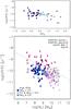 |
Fig. 6 Upper panel: specific star formation rate against Hi deficiency for Virgo SFDs. Crosses denote the average value in each bin of DefHI. Lower panel: specific star formation rates versus stellar masses. Blue symbols correspond to the Virgo SFDs, with the different shapes indicating the atomic hydrogen content of the galaxies as given by the Hi deficiency parameter. Symbols of comparison samples are the same used in Fig. 5. The dotted line indicates the star formation sequence defined by Schiminovich et al. (2007). |
The Sloan Digital Sky Survey (SDSS) provides high quality optical spectra covering the wavelength range 3800–9200 Å with a resolution of ~3 Å. The MPA-JHU collaboration provided measurements of emission-line fluxes and oxygen abundances for a sample of about 520 000 galaxies from the SDSS10, that we could use to derive the metal abundances of Virgo galaxies.
Because the discrepancies between the metallicities estimated from different calibrators can be as high as 70% (Yin et al. 2007; Kewley & Ellison 2008), we decided to derive the oxygen abundances following the method described in Hughes et al. (2013). Emission-line fluxes (obtained from the MPA-JHU catalogue) were corrected for internal and galactic extinction, Hα and Hβ lines were corrected for underlying stellar absorption, and then all line fluxes were normalised to Hα. The method of Hughes et al. (2013) combines the strong-line metallicity calibrations of McGaugh (1991), Zaritsky et al. (1994), Kewley & Dopita (2002), and two calibrations from Pettini & Pagel (2004): the O3N2 = [Oiii]λ5007/[Nii]λ6584 and the N2 = [NII]λ6584/Hα indices. The oxygen abundances given by the five methods are then converted into a base metallicity – O3N2 – via the conversion relations in Kewley & Ellison (2008), and the final metallicities are determined from the error-weighted average of all available estimates for each galaxy.
However, the only applicable calibrations for our sample of dwarfs were those based on the N2 and O3N2 indices. The other three methods could not be calculated since the [OII]λ3727 line is out of the measured wavelength range of the SDSS, and this line is required for the calibration based on the R23 = ([OII]λ3727 + [OIII]λλ4959,5007)/Hβ ratio. The final result was then obtained from either a single oxygen abundance estimate, or the error-weighted average of two estimates. Uncertainties in the final mean metallicities were derived using the typical errors of the applicable calibration relations, which were determined in Hughes et al. (2013) from the standard deviations of the scatter between each different calibration and the rest.
The final oxygen abundances range between 8.0~< 12 +log (O/H) ~< 8.8, and the mean error is estimated as 0.1 dex in 12 +log (O/H) units (see Table 2). The adopted solar metallicity is 12 + log (O/H)⊙ = 8.69 (Asplund et al. 2009).
Although the SDSS fibers sample the inner regions of the galaxies, dwarfs have been observed to have spatially homogeneous metallicity distribution (Kobulnicky & Skillman 1997; Croxall et al. 2009), therefore we are confident that our estimate is representative of the global metal content of the galaxies.
Metallicity estimates can vary depending on the calibration method used (Kewley & Ellison 2008), and if we want to compare the metal content of different galaxy samples we need to make sure that heavy element abundances are derived with the same method. KINGFISH and DGS metallicities are estimated following Pilyugin & Thuan (2005, hereafter PT05), based on the R23 ratio (Kennicutt et al. 2011; Rémy-Ruyer et al. 2014). Therefore we also derived PT05 oxygen abundances for 13 Virgo dwarfs for which [OII]λ3727 line fluxes measurements were available from the literature (Vílchez & Iglesias-Páramo 2003). We will use these values to facilitate comparison between the different surveys (see Sect. 9.3). The average difference between the method of Hughes et al. (2013) and PT05 is 0.14 dex. The PT05 metallicities are also listed in Table 2.
HeViCS BGC galaxies included in the HRS (Boselli et al. 2010) have oxygen abundances calculated in Hughes et al. (2013) and we list them in Table C.5.
5.5. Mid- and far-infrared observations from previous surveys
We also searched for mid- and far-infrared observations of Virgo SFDs in the IRAS Faint Source Catalogue (Moshir et al. 1990) and Point Source Catalogue (Helou & Walker 1988), and the ISOPHOT Virgo Cluster Catalogue (Tuffs et al. 2002; Popescu et al. 2002). We found both 60 and 100 μm detections for a total of 14 dwarfs. IRAS and ISO flux densities can also be found in the GOLDMine database. Therefore, we complement Herschel photometry with IRAS data for the following galaxies: VCC144, VCC324, VCC340, VCC699, VCC1437, VCC1554, VCC1575. ISOPHOT measurements are available for VCC1, VCC10, VCC87, VCC213, VCC1686, VCC1699, VCC1725.
6. Spectral energy distribution fitting
Assuming that dust grains are in local thermal equilibrium, the spectral energy
distribution (SED) of galaxies in the FIR-submm regime due to dust emission is found to be
well represented, in the optically thin limit, by a modified black body (MBB):
 (7)where B (ν,T) is the
Planck function, T is the dust temperature, and κν is the dust emissivity
or the grain absorption cross section per unit mass, expressed as a power-law function of
frequency: κν =
κ0(ν/ν0)β
(Hildebrand 1983). This simplified assumption does
not take into account that a galaxy can have a range of dust temperatures, and it cannot
fully describe the range of grain sizes of the different dust components (Bendo et al. 2012a, 2014). Nonetheless it is able to reproduce fairly well the observed large dust
grain properties of galaxies (Bianchi 2013), as long
as the function is not fitted to emission that includes stochastically-heated dust.
(7)where B (ν,T) is the
Planck function, T is the dust temperature, and κν is the dust emissivity
or the grain absorption cross section per unit mass, expressed as a power-law function of
frequency: κν =
κ0(ν/ν0)β
(Hildebrand 1983). This simplified assumption does
not take into account that a galaxy can have a range of dust temperatures, and it cannot
fully describe the range of grain sizes of the different dust components (Bendo et al. 2012a, 2014). Nonetheless it is able to reproduce fairly well the observed large dust
grain properties of galaxies (Bianchi 2013), as long
as the function is not fitted to emission that includes stochastically-heated dust.
The emissivity index β is a parameter that is related to the physical properties of the dust grains, such as the grain composition (the fraction of silicate versus graphite) and the grain structure (crystalline, amorphous, Mennella et al. 1995; Jager et al. 1998), and to the dust temperature (Mennella et al. 1998; Meny et al. 2007; Coupeaud et al. 2011). Laboratory studies of the two main interstellar dust analogs have shown that: i) carbonaceous grains have spectral indices varying between 1 and 2 according to their internal structure, with well-ordered graphitic grains characterised by β ~ 2, while lower values are found for carbonaceous grains with an amorphous structure (Preibisch et al. 1993; Colangeli et al. 1995; Mennella et al. 1995; Jager et al. 1998); ii) crystalline silicate grains have β ~ 2 (Mennella et al. 1998), and for amorphous silicates the range of variation of β at λ< 700μm is smaller (1.6 ≤ β ≤ 2.2), independently of grain temperature and composition (Coupeaud et al. 2011). In a study of amorphous silicates in the temperature range 10 <Td< 300 K at wavelengths between 0.1 μm and 2 mm, Boudet et al. (2005) report values of the emissivity spectral index between 1.5 and 2.5.
Planck Collaboration XIX (2011), Planck Collaboration XI (2014), Planck Collaboration Int. XVII (2014), Planck Collaboration Int. XXIII (2014) examined the FIR and millimetre emission in the galactic plane, the diffuse ISM, and over the whole sky, reporting β values in the range between 1.5 and 1.8, with a mean dust emissivity at high galactic latitudes βFIR = 1.59 ± 0.12 at ν ≥ 353 GHz (Planck Collaboration XI 2014), and a flattening of the dust SED at lower frequencies (ν< 353 GHz), with βFIR − βmm = 0.15 (Planck Collaboration Int. XVII 2014).
The typical values for β determined in global extragalactic studies fall within the range 1.0–2.5 (Galametz et al. 2011; Planck Collaboration XVII 2011; Boselli et al. 2012; Dale et al. 2012; Rémy-Ruyer et al. 2013). Nevertheless, in global studies the indices β inferred from MBB fitting are luminosity-averaged apparent values, and may not correspond to the intrinsic properties of the dust grains, but rather they can provide a measure of the apparent emissivity index (Kirkpatrick et al. 2014; Gordon et al. 2014; Hunt et al. 2014a). Indeed, because of the mixing of different dust temperatures along the line of sight, the presence of a dust component colder than the peak of the blackbody emission may produce a broader SED resulting in a fitted emissivity index shallower than the intrinsic β of the dust grain population (Malinen et al. 2011; Juvela & Ysard 2012). Fitted β are also found to vary with the intensity of the diffuse interstellar radiation field (ISRF, Hunt et al. 2014a). This implies that it can be difficult to assess the intrinsic dust grain properties on the basis of a single-temperature MBB fitting procedure.
Keeping in mind these issues, we adopted two approaches for the SED fitting procedure in order to investigate the range of β values that can better represent the FIR-submm SED of our sample of dwarf galaxies. First, we performed a single component modified black-body (MBB) fit using fixed values of the emissivity index, namely β = [ 1.0,1.2,1.5,1.8,2.0 ]; second, we repeated the SED fitting testing for each galaxy different values of β varying within the range [0, 3], and selected the value providing the best fit with the lowest residuals. Basically in this second approach the SED was fitted for a fixed β and the fitting process was repeated for all the values within 0 and 3 to determine the index that minimized the reduced χ2. The best fit to the data was obtained with the least squares fitting routines in the Interactive Data Language (IDL) MPFIT11 (Markwardt 2009). Our procedure is essentially a grid method for fitting temperature and normalization; such a technique tends to reduce the well-known degeneracy between temperature and β (e.g., Shetty et al. 2009a,b). These two approaches allow us to to test which values are needed to better describe the FIR-submm SED of our sample of dwarfs without a priori assumptions on the dust emissivity index value, similarly to what done in other studies of galaxies based on Herschel observations (Boselli et al. 2012; Rémy-Ruyer et al. 2013; Tabatabaei et al. 2014; Galametz et al. 2014; Kirkpatrick et al. 2014).
For this analysis, we considered only a subset of the sample (30 out of 49 galaxies) detected in four Herschel bands (100, 160, 250, and 350 μm) with S/N> 512. We restricted the SED fitting to data-points between 100 μm and 350 μm, because the submm emission at 500 μm in dwarf galaxies is usually found to exceed that expected from the model SED (Grossi et al. 2010; O’Halloran et al. 2010; Rémy-Ruyer et al. 2013). The origin of the 500 μm excess is still not clear and we will discuss this issue in more detail in Sect. 8.
 |
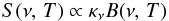
Fig. 7 Fractional residuals of the SED fitting at different wavelengths for β = 1.0,1.2,1.5,1.8,2.0. The fractional residual is calculated as the difference at each wavelength between the measured flux density and best-fit model divided by the best-fit model. The vertical dotted lines correspond to fractional residuals of 0 and ±0.1. The colours correspond to the four wavelengths considered for the SED fitting: 350 μm (red), 250 μm (black), 160 μm (green), 100 μm (blue). |
6.1. Fixed-β MBB fitting
To establish the overall best-fit β among the five adopted values β = [ 1.0,1.2,1.5,1.8,2.0 ] for the fixed-β MBB fitting procedure, we calculated the fractional residuals of the fits as the difference between the measured flux density Fν at 100, 160, 250, and 350 μm and the fitted function S(ν,T) divided by the best fit model. Then we compared the results for the five β values (Fig. 7). The dotted vertical lines indicates fractional residuals of 0 and ±0.1. The spread of the residuals for β = 1.5 is smaller than that for other emissivity indices, since most galaxies have residuals below 0.1 in all four bands (70%). Moreover, unlike other β values, the residuals of all four bands for β = 1.5, are centred on 0.
As mentioned in the previous section, measured dust emissivity variations among galaxies may be related to the issue of properly separating emission from warmer and colder dust components (Kirkpatrick et al. 2014; Bendo et al. 2014), implying that a colder diffuse dust could effectively be masked by warmer components in single thermal component SED fits between 100 and 500 μm (Xilouris et al. 2012). Therefore, as a further test, we repeated the fitting procedure with three data points only (160, 250 an 350 μm), using the 100 μm flux density as an upper limit, i.e. this data point was included in the SED fitting procedure only if the 160–350 μm fit resulted in an overprediction of the observed 100 μm measurement. Even in this case we obtained that β = 1.5 provided the best output model. Both results are compared in Fig. C.2, and this simple test shows that there are 7 galaxies for which performing a single-temperature MBB fit from 100 to 350 μm could hide the presence of a colder dust component blended with a warmer one (Kirkpatrick et al. 2014; Bendo et al. 2014).
Thus we will assume that for fixed β MBB fitting, β = 1.5 is the best overall solution for the emissivity. A modified black body with an emissivity index β = 1.5 is also found to better fit the SPIRE SED of the HRS galaxies (Boselli et al. 2012).
Free-β MBB fitting: best-fit parameters.
6.2. Free-β MBB fitting
To further explore the range of possible emissivity indices we repeated the fitting
procedure for each galaxy with different values of β within the range 0 to 3
in steps of 0.1, selecting the index that results in the lowest χ2. The best-fit
SED models are shown in Fig. C.1, and the results
from the fitting procedure are displayed in Table 3. Figure 8 shows that the emissivity index
varies substantially within the Virgo sample from β = 0.1 to 2.9. A few
galaxies have a low β value (<0.5); a flatter submm slope may be an indicator of the presence of
a submm excess (Rémy-Ruyer et al. 2013, see also
Sect. 8), or of an extremely low ISRF (Hunt et al. 2014a). Figure 8 shows the dust temperatures Td and β indices for our sample of
dwarfs (filled blue circles) and it indicates a clear anti-correlation between the two
parameters; the best-fit power-law which describes the relation between β and Td is overlaid
to the data13 (Fig. 8; blue dotted line) and it is given by
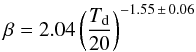 (8)which is close to what was found by Smith et al. (2012) in the outer regions of Andromeda
(red dashed line in Fig. 8), even though the dwarfs
extend to lower β values compared to M 31. A similar trend was also
derived by Davies et al. (2014) combining all
galaxies of the Virgo cluster later than S0 detected in the HeViCS survey (purple solid
line in Fig. 8), while a steeper power-law was found
by Rémy-Ruyer et al. (2013) in the DGS
(
(8)which is close to what was found by Smith et al. (2012) in the outer regions of Andromeda
(red dashed line in Fig. 8), even though the dwarfs
extend to lower β values compared to M 31. A similar trend was also
derived by Davies et al. (2014) combining all
galaxies of the Virgo cluster later than S0 detected in the HeViCS survey (purple solid
line in Fig. 8), while a steeper power-law was found
by Rémy-Ruyer et al. (2013) in the DGS
( ), characterised by overall higher dust
temperatures compared to the Virgo SFDs (
), characterised by overall higher dust
temperatures compared to the Virgo SFDs ( K). However, all these studies derived the
β −
Td relation using 100–500 μm data points in the SED
fitting procedure (and even 70 μm data for some DGS galaxies), while our SED
fittings were restricted to the wavelength range from 100 to 350 μm.
K). However, all these studies derived the
β −
Td relation using 100–500 μm data points in the SED
fitting procedure (and even 70 μm data for some DGS galaxies), while our SED
fittings were restricted to the wavelength range from 100 to 350 μm.
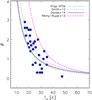 |
Fig. 8 Emissivity index plotted against dust temperature for the Virgo SFDs (filled blue dots). The dotted line shows the best-fit power law to our data set. For comparison we overlay the β − Td relation found in Andromeda (Smith et al. 2012), Virgo galaxies later than S0 (Davies et al. 2014), and DGS galaxies (Rémy-Ruyer et al. 2013). |
Although such an inverse relationship between β and Td is found in FIR-submm studies of different environments of the Milky Way (Veneziani et al. 2010), Andromeda (Smith et al. 2012), and in other samples of galaxies (Rémy-Ruyer et al. 2013; Cortese et al. 2014; Hughes et al. 2014), Shetty et al. (2009a) and Kelly et al. (2012) warn against the presence of a β − Td correlation as a physical property of the dust. These works suggest that there is a systematic degeneracy between β and Td that could be due to effect of noise on the SED fitting technique, as also shown in Tabatabaei et al. (2014). It follows that an artificial inverse β − Td correlation arises when a constant temperature along the line of sight is assumed to fit the properties of dust grains which are likely to span a range of dust temperatures.
6.3. Dust mass estimates for β = 1.5
Calculating dust masses of the galaxies for the different values of the emissivity index in the case of free-β SED fitting is not trivial. Indeed, as recently shown by Bianchi (2013), varying β while the value of dust opacity κ0 is kept fixed leads to wrong dust mass estimates, because κ0 is usually calibrated on a dust model with a well defined β. The correct determination of κν can be assessed only if one has a consistent dust model for the corresponding value of β, or by comparing dust mass estimates obtained from SED fitting with the ones obtained from other independent methods: e.g., using the amount of cold gas and metals, as proposed by James et al. (2002).
Therefore, given the difficulty of deriving the dust mass with a free emissivity index using the scaling relation in the Milky Way for β = 2 (Bianchi 2013), we decided to derive dust masses using the fixed-β fitting result, choosing β = 1.5 as the best compromise solution (see Sect. 6.1).
Fixed-β MBB fitting: dust temperatures for β = 1.5.
For 10 galaxies with only two data points (at λ ≤ 350 μm) we performed the SED
fitting with a fixed dust temperature using three values: Td = 23.9 K, the
median temperature obtained from the β = 1.5 fits for the 30 galaxies with better
quality photometry (Sect. 6.1); Td = 18.3 K, the
minimum value found in this subsample; Td = 21.1 K, an intermediate value
between the minimum and the median. Then we selected the temperature that provided the
best fit with the lowest χ2. The results for β = 1.5 are shown in Fig.
C.2, and the corresponding dust temperatures are
displayed in Table 4. The median dust temperature
of the 39 galaxies for which the SED fitting could be performed leaving Td as a free
parameter is  K.
K.
Dust masses for the 49 SFDs were then derived from the MBB fits according to
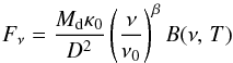 (9)with κ0 = 3.4
cm2 g-1 at λ = 250 μm, following the
prescription of Bianchi (2013). This value
reproduces the average emissivity of the Milky Way dust in the FIR-submm for
β = 1.5
(Bianchi 2013). Errors on the best-fit model
parameters (Td, Md) were
estimated via a bootstrap technique. For each galaxy we created 300 new sets of data
points randomly selected within the error bars of the observed fluxes. Then we repeated
the fitting procedure for each new data set and determined the best fitting parameters. We
calculated the 68% confidence interval in the parameter distributions and defined the
edges of this interval as the new upper and lower limits. The final uncertainties were
given by the difference between the original best-fit solution and the upper and lower
limit values from the bootstrap technique. Dust masses of Virgo SFDs are given in Table
214.
(9)with κ0 = 3.4
cm2 g-1 at λ = 250 μm, following the
prescription of Bianchi (2013). This value
reproduces the average emissivity of the Milky Way dust in the FIR-submm for
β = 1.5
(Bianchi 2013). Errors on the best-fit model
parameters (Td, Md) were
estimated via a bootstrap technique. For each galaxy we created 300 new sets of data
points randomly selected within the error bars of the observed fluxes. Then we repeated
the fitting procedure for each new data set and determined the best fitting parameters. We
calculated the 68% confidence interval in the parameter distributions and defined the
edges of this interval as the new upper and lower limits. The final uncertainties were
given by the difference between the original best-fit solution and the upper and lower
limit values from the bootstrap technique. Dust masses of Virgo SFDs are given in Table
214.
For an average rms of 6.7 mJy/beam at 250 μm (see Sect. 3.3) the 3σ dust mass detection limit assuming a dust
temperature K and a distance of 17 Mpc is
Md ≃ 4 ×
104 M⊙. Regarding FIR
non-detections, given the flux density derived in Sect. 3.3 (F250
= 4.5 mJy), the average dust mass calculated with the same parameters
(κ0,
 , D = 17 Mpc) corresponds to
Md = 8.7 ×
103 M⊙. The average dust mass
of the detected dwarfs is Md = 3 ×
105 M⊙.
, D = 17 Mpc) corresponds to
Md = 8.7 ×
103 M⊙. The average dust mass
of the detected dwarfs is Md = 3 ×
105 M⊙.
To perform a homogeneous comparison of the different surveys, we recalculated the dust masses of the DGS, KINGFISH, and BGC galaxies in the same way, i.e. we fitted a MBB with β = 1.5 to the Herschel flux densities and we determined the uncertainties on Td and Md with the bootstrap technique as explained above. Their values are given in the tables in Appendix C. Comparison with Rémy-Ruyer et al. (2013), where DGS and KINGFISH dust masses were calculated using a free-β emissivity, including the 500 μm data point in the SED fitting, shows that overall a fixed-β MBB fitting provides larger dust masses. For KINGFISH the difference between ours and their estimates peaks at 0.15 dex with a dispersion of ±0.05. Regarding the DGS, the logarithmic difference between the two estimates is scattered between –0.2 and +1.7 dex, however for 17 out of 27 galaxies the two measurements are consistent within the uncertainties.
7. Properties of Virgo SFDs: FIR detections versus FIR non-detections
Our analysis of the HeViCS data led to the selection of 49 SFDs with a FIR-submm counterpart. If we consider only dwarfs brighter than mB< 18 mag, the completeness limit of the VCC catalogue, this gives a detection rate of 43%.
The spatial distribution of Virgo SFDs can be seen in Fig. 1. Late-type dwarfs are usually located at larger distances from the centre of clusters and tend to avoid the densest regions (Binggeli et al. 1987). As expected, Herschel-detected SFDs are preferentially located in the less dense regions of the cluster. Only five dwarfs are within 2 degrees of M87 and only two are within 1.4 degree of M4915. The other detections are distributed between the LVC, the southern extension, the background clouds (W′, W, M), and the region between cluster A and B. The background clouds (M and W) contain about one third of the detected SFDs, according to the membership assignments of GOLDMine.
In this section we use global parameters of the whole sample of Virgo dwarfs to investigate whether FIR detections and non-detections have distinctive global properties.
Figure 9 compares the properties of Virgo late-type dwarfs brighter than mB< 18 mag, 49 with a FIR counterpart and 64 without. Stellar masses16, Hα fluxes, Hi masses, distances, and optical diameters (to derive Hi deficiencies), were taken from the GOLDMine database. The red histograms in the figure show the Herschel detections, while the filled grey histograms correspond to the non-detections. All histograms are normalized to their maximum values.
FIR-undetected galaxies have overall lower stellar masses, as it can be seen in the top left-hand panel of Fig. 9; the distribution peaks at log (M⋆/ M⊙) = 7.4, an order of magnitude lower compared to the detected sample. Only 44% of the dwarfs without a FIR counterpart have a Hα detection, and their Hα luminosities do not exceed ~106L⊙. The Hi mass distribution ranges for both samples between 107 and 109 M⊙, but FIR-emitting dwarfs have a higher fraction of Hi masses above 108 M⊙, and a higher detection rate at 21 cm (90% against 67%). Finally, in the last panel we compare the Hi deficiency (including 21 cm upper limits) for both type of galaxies, showing that the sample of undetected dwarfs have a larger fraction of objects with higher Hi deficiencies. Most of the Hi-poor FIR non-detections are found in cluster A and B, and in the region between these two substructures. Concerning the dwarf morphological types, BCDs show the highest detection rate (64%), followed by Sm (46%), and Im (24%) galaxies.
The main conclusion to infer from the figure is then that our detections are “biased” towards dwarfs with higher stellar and gas masses, less Hi-deficient, and more star-forming. Assuming the average dust-to-stellar mass ratio of dwarfs with a FIR counterpart (Md/M⋆ ~ 10-3), galaxies with log (M⋆/M⊙) = 7.4 (the peak of the grey histogram in Fig. 9) would have dust masses below the 3σ detection limit of the HeViCS survey determined in Sect. 6.3.
There is not enough information in the SDSS spectra to derive oxygen abundances for the non-detected galaxies, therefore we cannot assess whether dwarfs without a FIR counterpart are characterised by a lower metal content.
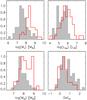 |
Fig. 9 Stellar mass, Hα luminosity, Hi mass, and Hi deficiency for the sample of FIR-detected (red histogram) and FIR-nondetected (filled grey histogram) Virgo dwarfs. All parameters are taken from the GOLDMine database, including the stellar masses of the Herschel-detected SFDs. |
8. The 500 μm excess
Several works have recently found that the SEDs of late-type galaxies exhibit emission at submm and millimetre (mm) wavelengths in excess of what is expected when a single modified Planck function is fitted. Such a submm excess, is preferentially found in dwarf/irregular/Magellanic morphological types (Lisenfeld et al. 2002; Galliano et al. 2003, 2005; Galametz et al. 2009, 2011; Bot et al. 2010; Rémy-Ruyer et al. 2013; Ciesla et al. 2014), with only a few cases of moderately low-metallicity spiral galaxies (Dumke et al. 2004; Bendo et al. 2006; Zhu et al. 2009).
In the analysis of the Science Demonstration Phase (SDP) data set of the HeViCS survey, we found that the 500 μm fluxes of two out of three SFDs tended to be underestimated by a single-temperature dust component fit, showing a submm excess emission (Grossi et al. 2010). Here we want to exploit the higher sensitivity of the completed survey, and the larger sample of detected dwarfs to derive more stringent constraints on the excess emission at 500 μm in Virgo SFDs.
We defined the 500 μm excess in the same way as has been done in other
studies (Dale et al. 2012; Rémy-Ruyer et al. 2013), i.e.:
 (10)where F500 is the
observed flux density and S500 the model flux density at 500
μm. We
determined ε500 for both fixed- and
free-β SED
fitting, including only 500 μm detections with S/N> 5.
Thus we used 23 out of 30 galaxies with the best FIR-submm photometry (see Sect. 6).
(10)where F500 is the
observed flux density and S500 the model flux density at 500
μm. We
determined ε500 for both fixed- and
free-β SED
fitting, including only 500 μm detections with S/N> 5.
Thus we used 23 out of 30 galaxies with the best FIR-submm photometry (see Sect. 6).
Variation of submm excess with MBB fitting procedure.
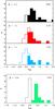 |
Fig. 10 500 μm fractional residuals for fixed- and free-β MBB fitting. The filled histograms correspond to the galaxies whose 500 μm excess is larger than the error on the flux density measurement. The fraction of dwarfs with a submm excess is displayed at the top-right corner of each panel. |
Figure 10 shows the variation with β of the fractional residuals at 500 μm. We assume that a 500 μm excess is observed if F500 − S500>σ500, where σ500 is the error on the flux density (filled histograms). As expected the number of galaxies with an excess decreases with β (Fig. 10). For β = 1.5, 67% of the detections present a 500 μm excess17, and even when β is allowed to vary, the fraction of galaxies with a stronger submm emission is still as significant (54%; Fig. 10). As the emissivity index decreases the fitted submm spectrum flattens at long wavelengths reducing the gap between the model SED and the observed flux density (see also Table 5). Therefore the selection of lower beta values would result in an overall lower fraction of galaxies with a detected submm excess.
If the excess emission is due to a change in the emissivity properties of the dust, one should expect to find a correlation with metallicity or other global properties of the galaxies. To probe whether such a link exists, we plot ε500 for the most extreme case (β = 2) as a function of metallicity, stellar mass, and SFR (left, central, and right panel of Fig. 11, respectively). We include also galaxies from the DGS and KINGFISH surveys showing a similar excess. Seven objects from the DGS and 9 from KINGFISH satisfy the conditions adopted to define the presence of a submm excess in Virgo dwarfs ((S/N)500> 5, F500 − S500>σ500). As regards the metallicity, we need to compare the Virgo dwarfs and DGS/KINGFISH (D+K) galaxies separately because of the different calibration used to derive the oxygen abundances. The left-hand panel shows that, despite the small number of objects, the excess is moderately anticorrelated with metallicity for the D+K samples but there is no correlation for Virgo SFDs. However we find a clear link between the excess with both stellar mass and star formation rate for all three surveys (Pearson coefficient correlation of –0.50 and –0.56, respectively). If stellar mass is a proxy for metallicity (Tremonti et al. 2004; Andrews & Martini 2013), the central panel of Fig. 11 suggests that the metallicities derived from the SDSS might be poorly constrained since our estimates were based on only two calibrations (see Sect. 5.4). The last panel shows that the excess is stronger in galaxies with a lower SFR.
Previous analysis of the link between the submm excess and global galaxy properties found different results: Bendo et al. (2006) reported an anticorrelation with the total infrared luminosity in NGC 4631, while Galametz et al. (2014) did not detect a clear trend between the relative excess at 870 μm and the 24 μm surface brightness in a set of KINGFISH galaxies.
In the study of the full DGS and KINGFISH samples, Rémy-Ruyer et al. (2013) found that about 45% of the 110 galaxies have an excess emission above the SED model at 500 μm (adopting a free-β MBB fitting), that this feature is mainly detected in dwarfs with metal abundances Z< 0.4 Z⊙, and the most metal-poor dwarfs of the DGS sample host the strongest excesses.
Indeed, the submm/mm excess is still an open issue that challenges standard dust models in this regime. Several hypotheses have been introduced so far to explain the peculiar dust properties at these wavelengths. Initially, the discovery of this feature in star-forming dwarfs was interpreted as evidence for a very cold dust component (Galliano et al. 2003, 2005; Galametz et al. 2009); however, the unphysically large dust masses implied by this scenario are difficult to reconcile with models of dust production and with the expected dust-to-gas ratios (Lisenfeld et al. 2002; Dumke et al. 2004; Bendo et al. 2006; Zhu et al. 2009; Planck Collaboration XIX 2011).
Alternatively, an enhanced abundance of hot, small dust grains (T ~ 30–50 K; sizes between 1.2 and 15 nm) with a low emissivity was suggested to explain the submm excess of the dwarf galaxy NGC 1569 (Lisenfeld et al. 2002) and of NGC 3310 (Zhu et al. 2009). In this scenario, large grain destruction by supernovae induced shocks in the ISM would produce the enhanced abundance of small grains.
Another hypothesis suggests that the emission arises from rotating very small dust grains (<1.2 nm) with permanent electric dipole moments located in the ionised gas (spinning dust). Grain collisions with the ionised gas and interactions with the UV radiation field can excite rotation of dust particles (Ferrara & Dettmar 1994; Draine & Lazarian 1998). For example, the predicted emission spectrum of spinning dust grains was invoked to account for the mm excess in the Small Magellanic Cloud (SMC; Bot et al. 2010; Planck Collaboration XVII 2011).
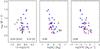 |
Fig. 11 500 μm fractional residuals for β = 2 against metallicity (left panel), stellar mass (central panel), and SFR (right panel) for the three samples of dwarfs: Virgo SFDs (blue dots), DGS (purple diamonds), and KINGFISH dwarfs (grey squares). Pearson correlation coefficients defining the degree of correlation are displayed in each panel. The fractional residuals of all three samples show a higher correlation with stellar mass and star formation rate. |
A population of magnetic dust grains (magnetite, maghemite, and metallic iron) with sizes smaller then 10 nm, mixed with “normal” dust grains has been recently suggested as an explanation for the SMC submm excess (Draine & Hensley 2012). Low-metallicity environments such as the SMC may provide more favorable conditions for the production and survival of iron-rich dust grains. Other studies reported that the properties of amorphous dust grains can depend strongly on temperature and that hotter dust grains can have low emissivity indices (Meny et al. 2007).
An emissivity variation with wavelength parameterised by a single-temperature MBB with a broken power-law has been advocated by Gordon et al. (2014) as a better model to explain the submm excess in the Magellanic clouds than the introduction of an additional population of very cold dust.
Finally, submm excess emission relative to a single-temperature MBB could not be necessarily related to peculiar dust properties, but rather it could be the consequence of temperature mixing along the line of sight (Shetty et al. 2009a), as also discussed in Sect. 6. Because the measured emissivity includes both the intrinsic emissivity of the dust and the range of temperatures of the different dust components, the temperature mixing could produce a shallower apparent β than what one would measure in the ideal case of a single-temperature component.
If the excess is the result of different grain properties our results may support two among the scenarios discussed above. The submm emission of small dust grains is expected to be lower than that of large dust grains, heated by both young and old stellar populations (see Sect. 9.1), thus it could be more easily detectable in galaxies with lower star formation rates and lower masses as we show in Fig. 11. On the other hand, the excess anticorrelation with stellar mass (hence with metallicity) may favour the Draine & Hensley (2012) scenario which assumes that metal-poor ISM may host a larger fraction of iron-rich dust grains emitting at submm/mm wavelengths.
9. Dust as a probe of galaxy evolution
9.1. Dust and star formation activity
Dust plays a fundamental role in regulating global star formation histories of galaxies and their evolution. Here we explore the relation between dust and star formation activity, comparing the properties of the Virgo SFDs to other Herschel surveys of dwarfs and late-type galaxies in different environments.
In Fig. 12, we plot dust masses Md versus SFRs in the Virgo dwarfs and the three comparison samples: KINGFISH, DGS, and HeViCS BGC. The galaxies in our sample except the DGS follow the best-fitting relation derived from da Cunha et al. (2010) for an IRAS-selected sample of local star-forming galaxies (solid line in Fig. 12). This correlation spans four orders of magnitude in both SFR and Md. It has been shown that the slope of the Md − SFR dependence can be related to the global Schmidt-Kennicutt law exponent (Hjorth et al. 2014). Evolutionary models of Hjorth et al. (2014) show that starbursting galaxies are expected to be located below the relation of da Cunha et al. (2010) because of the increasing contribution of supernovae to dust destruction in such systems. Dotted, dashed, and dot-dashed lines in Fig. 12 correspond to the evolution of the Md − SFR relation for different amounts of dust mass destroyed by a single supernova event: Mcl = 100, 500, 1500 M⊙ (see for details Hjorth et al. 2014). Although their models apply to more massive systems, this can give a hint to explain the scatter between the DGS and the other samples.
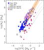 |
Fig. 12 Dust mass versus star formation rate for the Virgo SFDs (filled blue dots) compared to the KINGFISH spirals and dwarfs (small and large grey squares), and the DGS (red-purple triangles). The solid line shows the relation determined by da Cunha et al. (2010) for an IRAS selected sample of local star-forming galaxies. The orange shaded area stands for the dispersion of the relation. Evolution of the Md − SFR relation for different amounts of dust mass destroyed by a single supernova event – Mcl = 100, 500, 1500 M⊙ – is indicated by the dotted, dashed, dot-dashed lines, respectively (Hjorth et al. 2014). |
A large fraction of the radiation emitted from young stars is absorbed and re-emitted by dust. Whereas it is commonly assumed that warm dust is heated by young stars, the heating source of the diffuse cold dust emission in galaxies is still under debate (Boquien et al. 2011; Bendo et al. 2012a; Boselli et al. 2012; Foyle et al. 2013; Hughes et al. 2014). Herschel observations of nearby spiral galaxies suggest that the cold dust is heated by evolved stars rather than star forming regions (Bendo et al. 2010, 2012a; Boquien et al. 2011). On the other hand, diffuse dust might be less shielded from Hii regions in SFDs because of their less dense ISM and low-metallicity environment, possibly making young stars a dominant source of dust heating in these systems (Galametz et al. 2010).
To assess the dust heating mechanism in dwarfs we plot in Fig. 13 the F250/F350 colour as a function of SFR and stellar mass surface density for all samples. Spiral galaxies from the HeviCS BGC and KINGFISH samples are also included for comparison. SPIRE colours trace the properties of the Rayleigh-Jeans tail of the cold dust emission, and it has been shown that F250/F350 can be tightly correlated to the surface brightness of both the ionising and non-ionising interstellar radiation fields, giving hints about the dust heating mechanism (Boselli et al. 2012).
All samples are correlated with both parameters, although to different degrees, as shown by the Pearson correlation coefficients at the top left-hand corner of each panel. The strongest correlation with star formation surface density is found for the KINGFISH and DGS samples (r = 0.69). However the FIR colour of these dwarfs is also moderately correlated with the mass surface density (r = 0.48), suggesting that star formation is not the only mechanism responsible for dust heating in active SFDs. Regarding Virgo dwarfs, there is a moderate correlation between F250/F350 and the SFR (r = 0.39) and stellar mass (r = 0.45) surface densities. Most massive galaxies are more strongly correlated with the stellar surface density (r = 0.63) rather than with SFR (r = 0.47).
This analysis suggests that, consistent with what observed in other Herschel surveys (Boselli et al. 2012; Hughes et al. 2014; Bendo et al. 2014) both young and more evolved stellar populations contribute to the heating of the cold dust component in late-type dwarf galaxies, but the contribution of ionising interstellar radiation is stronger in more active SFDs.
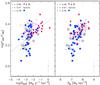 |
Fig. 13 Left panel: SPIRE colour F250/F350 against star formation rate surface density. Symbols are the same used in Fig. 12. The dotted line is a least square fit to the DGS and KINGFISH dwarf galaxies. Right panel: SPIRE colour F250/F350 against stellar mass surface density Pearson correlation coefficients for the different samples are displayed at the top-left corner of each panel. The mean error bars are displayed at the bottom-right corner of each panel. |
9.2. Dust scaling relations: evidence for dust stripping?
The dust-to-stellar mass ratio and the stellar mass are found to be mutually anticorrelated (da Cunha et al. 2010; Cortese et al. 2012), meaning that more massive galaxies have lower specific dust masses. This has been explained as the result of the correlation between sSFR and stellar mass: because of the higher star formation activity a large fraction of dust is formed, exceeding the amount of dust grains destroyed in the ISM (Schiminovich et al. 2007; da Cunha et al. 2010; Cortese et al. 2012). At higher stellar mass, the sSFR and gas fraction start decreasing and dust destruction begins to dominate over dust production, affecting the total dust mass of a galaxy. Such a trend is also confirmed by simulation of the time evolution of dust properties of late-type galaxies (Bekki 2013).
We explore the relation between the dust-to-stellar mass ratio and stellar mass in Fig. 14 (upper panel). The HeViCS BGC galaxies do show an anticorrelation between the two parameters. Concerning the dwarf samples, the relationship between dust fraction and stellar mass is less clear: Virgo SFDs form a parallel sequence to that defined by Virgo BGC objects, and their dust-to-stellar mass ratio is weakly anticorrelated with the stellar mass (r = −0.34), while for the other dwarfs there is no correlation between these two parameters. The DGS galaxies are mostly characterised by higher sSFRs and lower metal abundances compared to the Virgo SFDs, implying that they are in a different evolutionary stage. A combination of the more intense star formation activity (responsible for a higher dust destruction rates via supernova shocks; Hjorth et al. 2014) and outflows (Edmunds 2001; Dunne et al. 2011) could cause the lack of a correlation between dust fraction and stellar mass for this sample of galaxies.
Cortese et al. (2012) found that at stellar masses larger than 109 M⊙, Virgo cluster galaxies show systematically lower values of the dust-to-star mass ratio, compared to the HRS, suggesting that dust content has been affected by the cluster environment. The trend between Hi-normal and Hi-deficient HRS galaxies has been interpreted as an indication of ISM stripping (Cortese et al. 2012). In the lower panel of Fig. 14 the dust-to-stellar mass ratio is plotted against Hi deficiency for all Virgo galaxies. Galaxies with the highest Hi deficiencies (both dwarfs and spirals) do appear to have the lowest dust fractions, suggesting that environmental effects are affecting also the dust content. However, a larger sample of extremely Hi-deficient dwarfs would be needed to confirm that the same processes that make dwarfs gas deficient can also lower their dust masses.
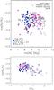 |
Fig. 14 Upper panel: dust-to-stellar mass ratios versus stellar masses of Virgo SFDs (filled dots, rings, ringed dots). The different shapes and gradation of blue correspond to three ranges of the Hi-deficiency parameter as defined in Fig. 6. For comparison, we show data for HeViCS BGC (purple diamonds), KINGFISH dwarfs and spirals (large and small grey squares), and DGS (red-purple triangles). Hi-deficient HeViCS BGC galaxies (DefHI ≥ 0.5) are indicated by a diamond with a cross. Lower panel: dust-to-stellar mass ratios versus Hi deficiency for Virgo SFDs and HeViCS BGC. |
 |
Fig. 15 Upper panel: dust-to-gas mass ratios against
metallicity for Virgo SFDs. Here we plot the oxygen abundance obtained from N2 e
O3N2 indices for the whole sample. Solid line indicates a linear scaling of the
Milky Way |
9.3. Environmental effects on the dust-to-gas mass ratio
The dust-to-gas mass ratio
(Md/Mg) gives an
indication of the enrichment of the gas by heavy elements produced in stars (C, O, Mg, Si,
Fe), the amount of metals that are locked in dust grains, and the net balance between the
production and growth of dust grains and their destruction in the ISM.
If the ratio of dust-to-metals in the ISM does not vary among galaxies, the relation
between
and the oxygen abundance O/H is expected to be linear (Edmunds 2001; Draine et al. 2007).
Several models predict the evolution of
as a function of metallicity (Dwek 1998; Lisenfeld & Ferrara 1998; Edmunds 2001; Hirashita et al.
2002). However, the relation between these two parameters at the very low
metallicity end (12 + log
(O/H)~< 8) is still an open issue, because
metal-poor dwarf galaxies do not follow the same linear dependence of metal-rich systems
(Draine et al. 2007; Galametz et al. 2011; Herrera-Camus et
al. 2012; Hunt et al. 2014b; Rémy-Ruyer et al. 2014).
Figure 15 explores the variation of
with nebular oxygen abundance for Virgo SFDs (upper panel) and comparison samples (lower
panel). We assumed that the total gas mass of the SFDs is given by the atomic component
only (with a correction for neutral helium Mg = 1.33
MHI), because of the lack of CO
measurements for Virgo and KINGFISH dwarfs, and the uncertainty in assessing the amount of
molecular gas in the metal-poor DGS galaxies (Rémy-Ruyer
et al. 2014). Because of the different methods used to derive metal abundances
(see Sect. 5.4), we need to analyse the samples of
dwarfs separately.
In the top-panel we use the oxygen abundances of the HeviCS dwarfs based on the N2 and
O3N2 indices. The Virgo SFDs are scattered along the
-metallicity
plane. The solid black line in the figure shows the linear scaling of the Milky Way
and metallicity (Draine et al. 2007), with dotted
and dashed lines showing a factor of 5 and 10 difference from MW, respectively. Most of
the Virgo dwarfs, especially the more gas-rich Virgo ones, have dust-to-gas ratios lower
than expected by linearly scaling the Milky Way values. Hi envelopes in dwarf
galaxies are known to be more extended than the stellar and dust components. Since all
dwarfs are unresolved by the ~3.́5 Arecibo beam, the ALFALFA catalogue provides the global
Hi content. Only a few Virgo dwarfs have been mapped at 21 cm, thus there is
not much information about the size of the Hi discs. A Very Large Array (VLA)
survey of Virgo BCDs (Hoffman et al. 2003) which
includes 5 of our dwarfs (VCC10, VCC24, VCC172, VCC340, VCC1437) found for these galaxies
Hi-to-optical diameter ratios, DHI/D25,
varying between 1.2 and 3.4, with a mean value around 2.
might be underestimated in some cases because of the different size of the gas compared to
the apertures adopted to measure the dust content (1.4 × R25), and
we will assess this issue in a future paper by comparing dust distribution to 21 cm maps
obtained for a subset of our galaxies (Coelho et al., in prep.).
Given the uncertainties in the correct estimate of the gas masses at this stage we cannot
draw firm conclusions on the relation between
and metallicity in our sample of Virgo dwarfs; nonetheless Fig. 15 suggests that Hi-deficient dwarfs have a higher
compared to those with a normal Hi content. VCC135 for example, the highest point
in the figure, has a dust-to-gas ratio which is about one order of magnitude higher than
what expected from the linear scaling of the Milky Way
and metallicity. The high
is a likely consequence of gas stripping by the cluster environment in these cases.
Furthermore, Hi-deficient dwarfs are preferentially found at higher metallicities, and the oxygen abundance progressively increase from Hi-normal to Hi-poor systems, similarly to what Hughes et al. (2013) found in nearby spiral galaxies. However, analysis of a larger, statistically significant sample of Hi-deficient dwarfs is needed to confirm this trend.
In the lower panel of Fig. 15, we compare Virgo
SFDs to KINGFISH and DGS, for which the metallicities have been derived with the PT05 method (see Sect. 5.4). Only Virgo dwarfs with [12
+log (O/H)] estimated according to PT05 can be compared to the other surveys without introducing systematic offsets
due to the different calibrations. Here the increase in
with the gas deficiency is still clear, despite the smaller number of galaxies shown.
Metal-poor dwarfs do not follow the linear scaling of the Milky Way metallicity and
.
Models that include the production and destruction of dust by supernovae, removal of dust
through outflows from galaxies, and dust production in the envelopes of stars (e.g., Hirashita et al. 2002; Asano et al. 2013; Zhukovska 2014) yield
non-linear relations between
and O/H, and may explain the breakdown of the trend at low metal abundances. As an
exercise we fit a broken power-law to the three samples of galaxies, similarly to Rémy-Ruyer et al. (2014). We fixed the power-law at
high metallicity to 1 and found a low-metallicity slope α = 2.23 ± 0.17 with a
break at [12 + log (O/H)]break =
8.36 ± 0.06 (orange line). For a more detailed analysis of the
variation of
with metallicity in the DGS and KINGFISH galaxies we refer the reader to Rémy-Ruyer et al. (2014).
The difference in the dust-to-gas ratio within different environments is also shown in
Fig. 16 where we plot
as a function of the stellar mass for all samples. The dwarfs with a larger gas content
(DGS, KINGFISH dwarfs, and Hi-normal Virgo SFDs) show a lower
for a given stellar mass, compared to the Hi-deficient Virgo dwarfs and the
HeViCS bright galaxies sample, which can be once again interpreted as the evidence of the
effects of the cluster environment on the gas component of low-mass systems.
10. Summary and conclusions
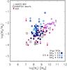 |
Fig. 16 Dust-to-gas mass ratio versus stellar mass for Virgo SFDs, KINGFISH dwarfs, DGS, and HeViCS BGC (with available molecular gas mass estimates). Symbols are the same as Fig. 14. Hi-deficient HeViCS BGC galaxies are indicated by a diamond with a cross. |
We used Herschel observations of the Virgo cluster taken as part of the Herschel Virgo Cluster Survey to investigate the FIR-submm properties of a sample of SFD galaxies and the effects of the cluster environment on the interstellar medium. We gathered optical, mid-infrared, and centimetre ancillary data from the literature to compare the dust content to stellar and gas masses, star formation rates, and metallicity. Among 140 late-type dwarf galaxies included in the HeViCS fields, we detected 49 objects at FIR-submm wavelengths. If we consider only the dwarfs brighter than mB = 18 mag, the completeness limit of the VCC, this gives a detection rate of 43%.
To assess the range of apparent β values that can better represent the shape of the FIR-submm SED of Virgo SFDs we performed MBB fitting of a subset of 30 galaxies (i.e. with detections in at least four Herschel bands) following two approaches. First we used a single MBB with fixed values of the emissivity index (β = [ 1.0,1.2,1.5,1.8,2.0 ]), secondly we repeated the SED fitting letting β vary between 0 and 3, and selecting the value which provided the best fit. With the first method (fixed-β), we found that the best-fit emissivity index minimising the fraction of residuals in four Herschel bands (100–350 μm) is β = 1.5. The range in dust temperature for β = 1.5 MBB fits is between 16.1 and 33.3 K, with a median of Td = 22.4 K. In the free-β case, the best-fit emissivities vary substantially among the sample, and we obtained values between 0.1 and 2.9. Dust masses of the 49 Herschel-detected dwarfs were calculated with β fixed at 1.5 following the calibration of the dust opacity of Bianchi (2013), and they range between 104.7 and 106.8 M⊙.
Stacking analysis of 64 SFDs without a 250 μm counterpart resulted in a 3.5σ detection with ⟨ F250 ⟩ = 4.2 mJy. Adopting β = 1.5 and Td = 22.4 K, the average dust mass of undetected dwarfs (brighter than the VCC completeness limit) corresponds to Md = 8.7 × 10³ M⊙ (at d = 17 Mpc), ~30 times lower than the mean value of the detected sample. Dwarfs without a FIR counterpart have lower stellar masses, lower Hα luminosities, and are more Hi-deficient.
Among the Herschel detections in all five bands (23 out of 49), 67% present an excess emission at 500 μm beyond the modified black-body model, assuming an emissivity index of β = 1.5. The fraction of Virgo dwarfs with a 500 μm excess decreases from β = 2 (88%) to β = 1 (42%). Even if a β-free SED modelling is applied, this fraction is still high (54%). The 500 μm fractional residuals show an inverse correlation with star formation rate and stellar masses. If the excess is due to different dust grain properties, our results may support either a scenario where the emission is produced by small dust grains (Lisenfeld et al. 2002; Bendo et al. 2006; Zhu et al. 2009), or by iron-rich dust grains which are expected to be more abundant in a metal-poor ISM (Draine & Hensley 2012).
To study the variations in the global properties of our sample due to environmental effects, we compared Virgo SFDs to other Herschel surveys targeting dwarfs in lower density environments such as the DGS and KINGFISH. We also included spiral galaxies from the HeViCS BGC and KINGFISH to investigate variations in dust properties with the morphological type.
From the analysis of SPIRE F250/F350 colour we infer that both young stars and more evolved stellar populations contribute to the heating of the cold dust component in Virgo SFD galaxies, and that the contribution of ionising insterstellar radiation is stronger in more active dwarfs such as those in the DGS and KINGFISH. On the other hand, old stars appear to dominate the dust heating process in the Virgo and KINGFISH spiral galaxies, consistent with previous studies.
We explored the relations between stellar mass and Hi fraction, sSFR, dust fraction, gas-to-dust ratio over a wide range of stellar masses (from 107 to 1011 M⊙) and morphological types. Increasingly more massive galaxies have progressively lower Hi gas fraction and sSFR, however Virgo galaxies are offset towards lower values of these parameters at a a given stellar mass, compared to similar galaxies in less dense environments.
A similar scaling relation is found for the dust content of spiral galaxies, but we do not find a clear correlation between M⋆/Md and M⋆ in the dwarf samples. These two parameters are marginally correlated only in Virgo SFDs, while in more active KINGFISH and DGS SFDs any correlation is lacking. We interpreted the lack of correlation in these systems as the consequence of a higher dust destruction rate and outflows due to the more intense star formation activity of these galaxies.
The most Hi-deficient dwarfs show lower sSFRs, Hi, and dust fractions
providing evidence for the effects of the cluster environment on the ISM and star formation
activity. However, we conclude that the amount of removed dust has to be lower compared to
the stripped Hi component, to explain the large
observed in the Hi-deficient systems. This is likely due to the larger extension of
the Hi discs compared to the dust distributions. As the Virgo star-forming dwarfs
are likely to be entering the cluster for the first time, longer time scales might be
necessary to strip or destroy the more centrally concentrated dust distribution and
transform these dwarfs into transition-type (De Looze et al.
2013) or early-type dwarfs (di Serego Alighieri et
al. 2013).
Online material
Appendix A: HeViCS BGC, DGS, KINGFISH stellar masses: comparison to previous estimates
Different stellar-mass estimation methods can yield mass values that disagree by factors up to ~2 (Kannappan & Gawiser 2007; McGaugh & Schombert 2014). To assess the reliability of our estimates based on MIR photometry, in this appendix we compare the stellar masses of the BGC, DGS, and KINGFISH samples to those derived by previous studies. In Fig. A.1 we show the results for the HeViCS BGC galaxies which are compared to Gavazzi et al. (2013a), where stellar masses were calculated using a relation combining the g − i colour and the i magnitude, calibrated on the MPA-JHU sample. We find a fair good agreement between the two estimates for this sample (purple diamonds), as we found for the HeViCS SFDs (blue dots, see Sect. 5.1): the residual distribution for the BGC sample (purple histogram) is slightly asymmetric, and peaks at 0.06 dex, with a dispersion of 0.13 dex.
Regarding the DGS, comparison to Rémy-Ruyer et al. (2013), where stellar masses were derived from IRAC 3.6 and 4.5 μm photometry following the method of Eskew et al. (2012), shows that our estimates are on average systematically smaller by a factor of ~0.17 ± 0.05 dex.
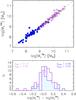 |
Fig. A.1 Upper panel: comparison between stellar masses
estimated in this work from WISE photometry,
|


Finally, comparison to the stellar masses of the KINGFISH sample calculated by Skibba et al. (2011) based on optical colours (Zibetti et al. 2009) shows that our estimates are on average systematically larger by a factor of ~0.5 dex. However for those galaxies with available SDSS photometry we compared our estimates with the stellar masses determined from i-band luminosities Li using the g − i colour-dependent stellar mass-to-light ratio relation (Zibetti et al. 2009), and found an average difference of 0.11 dex with a dispersion of 0.17 dex. The discrepancy is larger when the relations using B − V, or B − R colours are used for those objects without SDSS photometry.
Appendix B: Two-component modified black-body SED fitting
Analysing two-component MBB models is important to begin to assess the dust temperature mixing along the line of sight, which could in principle lead to a lower β value when the SED fitting takes only into account one dust component. We combined MIR photometry from the literature with our FIR-submm observation for a subset of 14 galaxies with available mid-infrared (MIR) observations (see Sect. 5.5), and we fitted the SED using two modified black-body models, one for the warm component and one for the cold component. We fixed the emissivity index of the warm component at βw = 2, an approximation of the opacity in the standard Li & Draine (2001) dust models, and that of the cold component at βc = 1.5. We used the 22 μm data point in the fit as an upper limit to better constrain the warm dust modified blackbody. The result is shown in Fig. B.1. For two galaxies an additional dust component is not necessary to fit observations at 60 and 100 μm (VCC213, VCC1725).
The temperature of the warm component ranges between 43 and 54 K, while the change in the cold dust temperature, compared to a single temperature MBB fit (see Tables B.1 and 4), varies between –0.1 and –4.3 K.
Two-component MBB SED fitting for the subset of Virgo dwarfs with IRAS and ISO photometry.
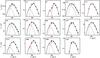 |
Fig. B.1 2-component MBB fits for 14 dwarfs with available IRAS and ISO photometry. Filled red dots correspond to IRAS or ISO data, while black dots show Herschel photometry. The emissivity index of the cold dust component (dotted line) is fixed at βc = 1.5, while the warm dust component (dashed line) has βw = 2.0. The VCC catalogue ID is given at the upper-left corner of each plot. |
Appendix C: Data Tables and SED fitting results
Herschel photometry of the sample of Virgo star-forming dwarf galaxies.
Stellar masses, Hi masses, dust masses, star formation rates, metallicities, Hi deficiency, and distances of the 27 objects selected from the Dwarf Galaxy Survey.
Stellar masses, Hi masses, dust masses, star formation rates, metallicities, Hi deficiency, and distances of the KINGFISH dwarf galaxy sample.
Stellar masses, Hi masses, dust masses, star formation rates, H2 masses, Hi deficiency and distances of KINGFISH spiral galaxies (from Sa to Sd).
Stellar masses, Hi masses, dust masses, star formation rates, H2 masses, Hi deficiency, and distances of HeViCS BGC galaxies.
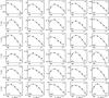 |
Fig. C.1 Free-β MBB fitting for 30 Virgo SFDs detected in four bands (100, 160, 250, 350 μm). The best-fit emissivity index is displayed at the upper-right corner, and the VCC catalogue ID is given at the lower-left corner of each plot. |
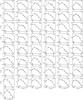 |
Fig. C.2 Fixed-β MBB fitting (β = 1.5) for the
whole sample of Virgo dwarfs detected with Herschel (black solid
line). The reduced χ2 value of the fitting is
displayed at the upper-right corner of each plot. The VCC catalogue ID is given at
the lower-left corner of each plot. The red dotted lines correspond to the MBB
obtained by fitting only three points of the SED (160–350 μm) instead of four
points (100–350 μm). The three-point fits are shown only for
those galaxies where the difference between the dust masses derived with the two
methods, |

http://herschel.esac.esa.int/twiki/bin/view/Public/SpireCalibrationWeb
herschel.esac.esa.int/Docs/SPIRE/spire_handbook.pdf
This corresponds to GOLDMine morphological types from 11 to 17.
The Wen et al. (2013) relation between stellar mass and 3.4 μm luminosity was derived by matching the WISE All-Sky Release Catalogue (http://wise2.ipac.caltech.edu/docs/release/allsky/) and the MPA-JHU Sloan Digital Sky Survey catalogue (http://www.mpa-garching.mpg.de/SDSS/DR7/), where the stellar masses were calculated by fitting the u,g,r,i,z photometry with a large number of model SEDs constructed from the Bruzual & Charlot (2003) population synthesis code which assumes a Chabrier (2003) initial mass function (IMF).
This correction is due to a calibration discrepancy between the WISE photometric standard “blue” stars and “red” galaxies (e.g., star-forming systems) and it must be applied only to W4 flux densities.
The relation of Wen et al. (2014) is calibrated assuming a Kroupa (2001) IMF. Because the SFRs calculated with this IMF yields nearly identical results to those derived with a Chabrier (2003) IMF (Chomiuk & Povich 2011; Kennicutt & Evans 2012), we avoid rescaling Eq. (4) to a Chabrier IMF.
Note that we also included VCC741, VCC1179, and VCC1273 despite having a lower S/N detection at 100 μm.
Galaxies with the lowest emissivity indices (β ≤ 0.3) are not included in the fit.
For the 7 galaxies discussed in Sect. 6.1 which might host a colder dust component blended with a warmer one, the four point fit might underestimate the dust mass by a factor of 0.1–0.2 dex.
Low FIR detection rates in cluster A and B are also observed in the Virgo early-type dwarf population (di Serego Alighieri et al. 2013).
To facilitate the comparison, in this section we use stellar masses from GOLDMine (derived from optical photometry (g, i) as explained in Sect. 5.1.1) for both detected and undetected galaxies, because we did not measure WISE 3.4 μm photometry for Virgo SFDs without a FIR counterpart.
In the case of the three-point SED fitting procedure discussed in Sect. 6.1 (where the 100 μm data point is used as an upper limit), the fraction of dwarfs with a submm excess decreases only marginally, with percentages of 79%, 63%, and 33% for β = 2.0, 1.5, and 1.0, respectively.
Acknowledgments
M.G. gratefully acknowledges support from the Science and Technology Foundation (FCT, Portugal) through the research grant PTDC/CTE-AST/111140/2009. S.B., E.C., and L.K.H. acknowledge support from PRIN-INAF 2012/2013. SCM and ARR acknowledge support from the Agence Nationale de la Recherche (ANR) through the programme SYMPATICO (Program Blanc Projet ANR-11-BS56-0023). T.M.H. gratefully acknowledges the financial support from the Belgian Science Policy Office (BELSPO) in the frame of the PRODEX project C90370 (Herschel-PACS Guaranteed Time and Open Time Programs: Science Exploitation). I.D.L. is a postdoctoral researcher of the FWO-Vlaanderen (Belgium). Funding for SDSS-III has been provided by the Alfred P. Sloan Foundation, the Participating Institutions, the National Science Foundation, and the US Department of Energy Office of Science. The SDSS-III web site is http://www.sdss3.org/. SDSS-III is managed by the Astrophysical Research Consortium for the Participating Institutions of the SDSS-III Collaboration including the University of Arizona, the Brazilian Participation Group, Brookhaven National Laboratory, Carnegie Mellon University, University of Florida, the French Participation Group, the German Participation Group, Harvard University, the Instituto de Astrofisica de Canarias, the Michigan State/Notre Dame/JINA Participation Group, Johns Hopkins University, Lawrence Berkeley National Laboratory, Max Planck Institute for Astrophysics, Max Planck Institute for Extraterrestrial Physics, New Mexico State University, New York University, Ohio State University, Pennsylvania State University, University of Portsmouth, Princeton University, the Spanish Participation Group, University of Tokyo, University of Utah, Vanderbilt University, University of Virginia, University of Washington, and Yale University. This publication makes use of data products from the Wide-field Infrared Survey Explorer, which is a joint project of the University of California, Los Angeles, and the Jet Propulsion Laboratory/California Institute of Technology, funded by the National Aeronautics and Space Administration. We thank the many members of the ALFALFA team who have contributed to the acquisition and processing of the ALFALFA dataset over the last six years. The Arecibo Observatory is operated by SRI International under a cooperative agreement with the National Science Foundation (AST-1100968), and in alliance with Ana G. Mandez-Universidad Metropolitana, and the Universities Space Research Association. This research has made use of the NASA/IPAC Extragalactic Database (NED) which is operated by the Jet Propulsion Laboratory, California Institute of Technology, under contract with the National Aeronautics and Space Administration.
References
- Ackermann, M., Ajello, M., Baldini, L., et al. 2011, ApJ, 726, 81 [NASA ADS] [CrossRef] [Google Scholar]
- Andrews, B. H., & Martini, P. 2013, ApJ, 765, 140 [NASA ADS] [CrossRef] [Google Scholar]
- Asano, R. S., Takeuchi, T. T., Hirashita, H., & Nozawa, T. 2013, MNRAS, 432, 637 [NASA ADS] [CrossRef] [Google Scholar]
- Asplund, M., Grevesse, N., Sauval, A. J., & Scott, P. 2009, ARA&A, 47, 481 [NASA ADS] [CrossRef] [Google Scholar]
- Auld, R., Bianchi, S., Smith, M. W. L., et al. 2013, MNRAS, 428, 1880 [NASA ADS] [CrossRef] [Google Scholar]
- Balog, Z., Müller, T., Nielbock, M., et al. 2013, Exper. Astron. [arXiv:1309.6099] [Google Scholar]
- Bekki, K. 2013, MNRAS, 432, 2298 [NASA ADS] [CrossRef] [Google Scholar]
- Bendo, G. J., Dale, D. A., Draine, B. T., et al. 2006, ApJ, 652, 283 [NASA ADS] [CrossRef] [Google Scholar]
- Bendo, G. J., Wilson, C. D., Pohlen, M., et al. 2010, A&A, 518, L65 [NASA ADS] [CrossRef] [EDP Sciences] [Google Scholar]
- Bendo, G. J., Boselli, A., Dariush, A., et al. 2012a, MNRAS, 419, 1833 [NASA ADS] [CrossRef] [Google Scholar]
- Bendo, G. J., Galliano, F., & Madden, S. C. 2012b, MNRAS, 423, 197 [NASA ADS] [CrossRef] [Google Scholar]
- Bendo, G. J., Griffin, M. J., Bock, J. J., et al. 2013, MNRAS, 433, 3062 [NASA ADS] [CrossRef] [Google Scholar]
- Bendo, G. J., Baes, M., Bianchi, S., et al. 2014, MNRAS, submitted [arXiv:1409.1815] [Google Scholar]
- Bianchi, S. 2013, A&A, 552, A89 [NASA ADS] [CrossRef] [EDP Sciences] [Google Scholar]
- Binggeli, B., Sandage, A., & Tammann, G. A. 1985, AJ, 90, 1681 [NASA ADS] [CrossRef] [Google Scholar]
- Binggeli, B., Tammann, G. A., & Sandage, A. 1987, AJ, 94, 251 [NASA ADS] [CrossRef] [Google Scholar]
- Binggeli, B., Popescu, C. C., & Tammann, G. A. 1993, A&AS, 98, 275 [NASA ADS] [Google Scholar]
- Bohlin, R. C., Savage, B. D., & Drake, J. F. 1978, ApJ, 224, 132 [NASA ADS] [CrossRef] [Google Scholar]
- Bolatto, A. D., Leroy, A. K., Rosolowsky, E., Walter, F., & Blitz, L. 2008, ApJ, 686, 948 [NASA ADS] [CrossRef] [Google Scholar]
- Boquien, M., Calzetti, D., Combes, F., et al. 2011, AJ, 142, 111 [NASA ADS] [CrossRef] [Google Scholar]
- Boselli, A., & Gavazzi, G. 2006, PASP, 118, 517 [NASA ADS] [CrossRef] [Google Scholar]
- Boselli, A., Lequeux, J., & Gavazzi, G. 2002, A&A, 384, 33 [NASA ADS] [CrossRef] [EDP Sciences] [Google Scholar]
- Boselli, A., Boissier, S., Cortese, L., & Gavazzi, G. 2008, ApJ, 674, 742 [NASA ADS] [CrossRef] [Google Scholar]
- Boselli, A., Eales, S., Cortese, L., et al. 2010, PASP, 122, 261 [NASA ADS] [CrossRef] [Google Scholar]
- Boselli, A., Ciesla, L., Cortese, L., et al. 2012, A&A, 540, A54 [NASA ADS] [CrossRef] [EDP Sciences] [Google Scholar]
- Boselli, A., Cortese, L., & Boquien, M. 2014a, A&A, 564, A65 [NASA ADS] [CrossRef] [EDP Sciences] [Google Scholar]
- Boselli, A., Cortese, L., Boquien, M., et al. 2014b, A&A, 564, A67 [NASA ADS] [CrossRef] [EDP Sciences] [Google Scholar]
- Bot, C., Ysard, N., Paradis, D., et al. 2010, A&A, 523, A20 [NASA ADS] [CrossRef] [EDP Sciences] [Google Scholar]
- Boudet, N., Mutschke, H., Nayral, C., et al. 2005, ApJ, 633, 272 [NASA ADS] [CrossRef] [Google Scholar]
- Boulanger, F., Abergel, A., Bernard, J.-P., et al. 1996, A&A, 312, 256 [NASA ADS] [Google Scholar]
- Brosch, N., Almoznino, E., & Heller, A. B. 2004, MNRAS, 349, 357 [NASA ADS] [CrossRef] [Google Scholar]
- Brown, M. J. I., Moustakas, J., Smith, J.-D. T., et al. 2014, ApJS, 212, 18 [Google Scholar]
- Bruzual, G., & Charlot, S. 2003, MNRAS, 344, 1000 [NASA ADS] [CrossRef] [Google Scholar]
- Calzetti, D., Armus, L., Bohlin, R. C., et al. 2000, ApJ, 533, 682 [NASA ADS] [CrossRef] [Google Scholar]
- Calzetti, D., Wu, S.-Y., Hong, S., et al. 2010, ApJ, 714, 1256 [NASA ADS] [CrossRef] [Google Scholar]
- Chabrier, G. 2003, PASP, 115, 763 [NASA ADS] [CrossRef] [Google Scholar]
- Chomiuk, L., & Povich, M. S. 2011, AJ, 142, 197 [NASA ADS] [CrossRef] [Google Scholar]
- Chung, A., van Gorkom, J. H., Kenney, J. D. P., Crowl, H., & Vollmer, B. 2009, AJ, 138, 1741 [NASA ADS] [CrossRef] [Google Scholar]
- Ciesla, L., Boselli, A., Smith, M. W. L., et al. 2012, A&A, 543, A161 [NASA ADS] [CrossRef] [EDP Sciences] [Google Scholar]
- Ciesla, L., Boquien, M., Boselli, A., et al. 2014, A&A, 565, A128 [Google Scholar]
- Colangeli, L., Mennella, V., Bussoletti, E., et al. 1995, Planet. Space Sci., 43, 1263 [NASA ADS] [CrossRef] [Google Scholar]
- Corbelli, E., Bianchi, S., Cortese, L., et al. 2012, A&A, 542, A32 [NASA ADS] [CrossRef] [EDP Sciences] [Google Scholar]
- Cortese, L., Davies, J. I., Pohlen, M., et al. 2010, A&A, 518, L49 [NASA ADS] [CrossRef] [EDP Sciences] [Google Scholar]
- Cortese, L., Catinella, B., Boissier, S., Boselli, A., & Heinis, S. 2011, MNRAS, 415, 1797 [NASA ADS] [CrossRef] [Google Scholar]
- Cortese, L., Ciesla, L., Boselli, A., et al. 2012, A&A, 540, A52 [NASA ADS] [CrossRef] [EDP Sciences] [Google Scholar]
- Cortese, L., Fritz, J., Bianchi, S., et al. 2014, MNRAS, 440, 942 [NASA ADS] [CrossRef] [Google Scholar]
- Coupeaud, A., Demyk, K., Meny, C., et al. 2011, A&A, 535, A124 [NASA ADS] [CrossRef] [EDP Sciences] [Google Scholar]
- Cowie, L. L., Songaila, A., Hu, E. M., & Cohen, J. G. 1996, AJ, 112, 839 [Google Scholar]
- Crowl, H. H., Kenney, J. D. P., van Gorkom, J. H., & Vollmer, B. 2005, AJ, 130, 65 [NASA ADS] [CrossRef] [Google Scholar]
- Croxall, K. V., van Zee, L., Lee, H., et al. 2009, ApJ, 705, 723 [NASA ADS] [CrossRef] [Google Scholar]
- da Cunha, E., Eminian, C., Charlot, S., & Blaizot, J. 2010, MNRAS, 403, 1894 [NASA ADS] [CrossRef] [Google Scholar]
- Dale, D. A., Aniano, G., Engelbracht, C. W., et al. 2012, ApJ, 745, 95 [NASA ADS] [CrossRef] [Google Scholar]
- Davies, J. I., Baes, M., Bendo, G. J., et al. 2010, A&A, 518, L48 [NASA ADS] [CrossRef] [EDP Sciences] [Google Scholar]
- Davies, J. I., Bianchi, S., Cortese, L., et al. 2012, MNRAS, 419, 3505 [NASA ADS] [CrossRef] [Google Scholar]
- Davies, J. I., Bianchi, S., Baes, M., et al. 2014, MNRAS, 438, 1922 [NASA ADS] [CrossRef] [Google Scholar]
- De Looze, I., Baes, M., Boselli, A., et al. 2013, MNRAS, 436, 1057 [NASA ADS] [CrossRef] [Google Scholar]
- di Serego Alighieri, S., Bianchi, S., Pappalardo, C., et al. 2013, A&A, 552, A8 [NASA ADS] [CrossRef] [EDP Sciences] [Google Scholar]
- Dowell, C. D., Pohlen, M., Pearson, C., et al. 2010, in SPIE Conf. Ser., 7731, 36 [Google Scholar]
- Doyon, R., & Joseph, R. D. 1989, MNRAS, 239, 347 [NASA ADS] [Google Scholar]
- Draine, B. T., & Lazarian, A. 1998, ApJ, 494, L19 [NASA ADS] [CrossRef] [Google Scholar]
- Draine, B. T., & Hensley, B. 2012, ApJ, 757, 103 [CrossRef] [Google Scholar]
- Draine, B. T., Dale, D. A., Bendo, G., et al. 2007, ApJ, 663, 866 [NASA ADS] [CrossRef] [Google Scholar]
- Dumke, M., Krause, M., & Wielebinski, R. 2004, A&A, 414, 475 [NASA ADS] [CrossRef] [EDP Sciences] [Google Scholar]
- Dunne, L., Gomez, H. L., da Cunha, E., et al. 2011, MNRAS, 417, 1510 [NASA ADS] [CrossRef] [Google Scholar]
- Dwek, E. 1998, ApJ, 501, 643 [NASA ADS] [CrossRef] [Google Scholar]
- Edmunds, M. G. 2001, MNRAS, 328, 223 [NASA ADS] [CrossRef] [Google Scholar]
- Eskew, M., Zaritsky, D., & Meidt, S. 2012, AJ, 143, 139 [NASA ADS] [CrossRef] [Google Scholar]
- Ferrara, A., & Dettmar, R.-J. 1994, ApJ, 427, 155 [NASA ADS] [CrossRef] [Google Scholar]
- Foyle, K., Natale, G., Wilson, C. D., et al. 2013, MNRAS, 432, 2182 [NASA ADS] [CrossRef] [Google Scholar]
- Ftaclas, C., Struble, M. F., & Fanelli, M. N. 1984, ApJ, 282, 19 [NASA ADS] [CrossRef] [Google Scholar]
- Fumagalli, M., Krumholz, M. R., Prochaska, J. X., Gavazzi, G., & Boselli, A. 2009, ApJ, 697, 1811 [NASA ADS] [CrossRef] [Google Scholar]
- Fumagalli, M., da Silva, R. L., & Krumholz, M. R. 2011, ApJ, 741, L26 [NASA ADS] [CrossRef] [Google Scholar]
- Galametz, M., Madden, S., Galliano, F., et al. 2009, A&A, 508, 645 [NASA ADS] [CrossRef] [EDP Sciences] [Google Scholar]
- Galametz, M., Madden, S. C., Galliano, F., et al. 2010, A&A, 518, L55 [NASA ADS] [CrossRef] [EDP Sciences] [Google Scholar]
- Galametz, M., Madden, S. C., Galliano, F., et al. 2011, A&A, 532, A56 [NASA ADS] [CrossRef] [EDP Sciences] [Google Scholar]
- Galametz, M., Albrecht, M., Kennicutt, R., et al. 2014, MNRAS, 439, 2542 [NASA ADS] [CrossRef] [Google Scholar]
- Galliano, F., Madden, S. C., Jones, A. P., et al. 2003, A&A, 407, 159 [NASA ADS] [CrossRef] [EDP Sciences] [Google Scholar]
- Galliano, F., Madden, S. C., Jones, A. P., Wilson, C. D., & Bernard, J. 2005, A&A, 434, 867 [NASA ADS] [CrossRef] [EDP Sciences] [Google Scholar]
- Gavazzi, G., Boselli, A., Scodeggio, M., Pierini, D., & Belsole, E. 1999, MNRAS, 304, 595 [NASA ADS] [CrossRef] [Google Scholar]
- Gavazzi, G., Boselli, A., Pedotti, P., Gallazzi, A., & Carrasco, L. 2002, A&A, 396, 449 [NASA ADS] [CrossRef] [EDP Sciences] [Google Scholar]
- Gavazzi, G., Boselli, A., Donati, A., Franzetti, P., & Scodeggio, M. 2003, A&A, 400, 451 [NASA ADS] [CrossRef] [EDP Sciences] [Google Scholar]
- Gavazzi, G., Boselli, A., van Driel, W., & O’Neil, K. 2005, A&A, 429, 439 [NASA ADS] [CrossRef] [EDP Sciences] [Google Scholar]
- Gavazzi, G., Fumagalli, M., Galardo, V., et al. 2012, A&A, 545, A16 [NASA ADS] [CrossRef] [EDP Sciences] [Google Scholar]
- Gavazzi, G., Fumagalli, M., Fossati, M., et al. 2013a, A&A, 553, A89 [NASA ADS] [CrossRef] [EDP Sciences] [Google Scholar]
- Gavazzi, G., Savorgnan, G., Fossati, M., et al. 2013b, A&A, 553, A90 [NASA ADS] [CrossRef] [EDP Sciences] [Google Scholar]
- Gavazzi, G., Franzetti, P., & Boselli, A. 2014 [arXiv:1401.8123] [Google Scholar]
- Gil de Paz, A., Madore, B. F., & Pevunova, O. 2003, ApJS, 147, 29 [NASA ADS] [CrossRef] [Google Scholar]
- Giovanardi, C., Helou, G., Salpeter, E. E., & Krumm, N. 1983, ApJ, 267, 35 [NASA ADS] [CrossRef] [Google Scholar]
- Giovanelli, R., Haynes, M. P., Kent, B. R., et al. 2005, AJ, 130, 2598 [NASA ADS] [CrossRef] [Google Scholar]
- Gomez, H. L., Baes, M., Cortese, L., et al. 2010, A&A, 518, L45 [NASA ADS] [CrossRef] [EDP Sciences] [Google Scholar]
- Gordon, K. D., Roman-Duval, J., Bot, C., et al. 2014, ApJ, submitted [arXiv:1406.6066] [Google Scholar]
- Gould, R. J., & Salpeter, E. E. 1963, ApJ, 138, 393 [NASA ADS] [CrossRef] [Google Scholar]
- Griffin, M. J., Abergel, A., Abreu, A., et al. 2010, A&A, 518, L3 [Google Scholar]
- Grossi, M., Hunt, L. K., Madden, S., et al. 2010, A&A, 518, L52 [NASA ADS] [CrossRef] [EDP Sciences] [Google Scholar]
- Gunn, J. E., & Gott, III, J. R. 1972, ApJ, 176, 1 [NASA ADS] [CrossRef] [Google Scholar]
- Haynes, M. P., & Giovanelli, R. 1984, AJ, 89, 758 [NASA ADS] [CrossRef] [Google Scholar]
- Haynes, M. P., Giovanelli, R., Martin, A. M., et al. 2011, AJ, 142, 170 [NASA ADS] [CrossRef] [Google Scholar]
- Helou, G., & Walker, D. W. 1988, Infrared astronomical satellite (IRAS) catalogs and atlases, The small scale structure catalog, 7 [Google Scholar]
- Herrera-Camus, R., Fisher, D. B., Bolatto, A. D., et al. 2012, ApJ, 752, 112 [NASA ADS] [CrossRef] [EDP Sciences] [Google Scholar]
- Hildebrand, R. H. 1983, QJRAS, 24, 267 [NASA ADS] [Google Scholar]
- Hirashita, H., Tajiri, Y. Y., & Kamaya, H. 2002, A&A, 388, 439 [NASA ADS] [CrossRef] [EDP Sciences] [Google Scholar]
- Hjorth, J., Gall, C., & Michałowski, M. J. 2014, ApJ, 782, L23 [NASA ADS] [CrossRef] [Google Scholar]
- Hoffman, G. L., Glosson, J., Helou, G., Salpeter, E. E., & Sandage, A. 1987, ApJS, 63, 247 [NASA ADS] [CrossRef] [Google Scholar]
- Hoffman, G. L., Helou, G., Salpeter, E. E., & Lewis, B. M. 1989, ApJ, 339, 812 [NASA ADS] [CrossRef] [Google Scholar]
- Hoffman, G. L., Brosch, N., Salpeter, E. E., & Carle, N. J. 2003, AJ, 126, 2774 [NASA ADS] [CrossRef] [Google Scholar]
- Hollenbach, D., & Salpeter, E. E. 1971, ApJ, 163, 155 [NASA ADS] [CrossRef] [Google Scholar]
- Huang, S., Haynes, M. P., Giovanelli, R., & Brinchmann, J. 2012, ApJ, 756, 113 [NASA ADS] [CrossRef] [Google Scholar]
- Hughes, T. M., Cortese, L., Boselli, A., Gavazzi, G., & Davies, J. I. 2013, A&A, 550, A115 [NASA ADS] [CrossRef] [EDP Sciences] [Google Scholar]
- Hughes, T. M., Baes, M., Fritz, J., et al. 2014, A&A, 565, A4 [NASA ADS] [CrossRef] [EDP Sciences] [Google Scholar]
- Hunt, L., Magrini, L., Galli, D., et al. 2012, MNRAS, 427, 906 [NASA ADS] [CrossRef] [Google Scholar]
- Hunt, L. K., Draine, B. T., Bianchi, S., et al. 2014a, A&A, in press DOI: 10.1051/0004-6361/201424734 [Google Scholar]
- Hunt, L. K., Testi, L., Casasola, V., et al. 2014b, A&A, 561, A49 [NASA ADS] [CrossRef] [EDP Sciences] [Google Scholar]
- Jager, C., Mutschke, H., & Henning, T. 1998, A&A, 332, 291 [NASA ADS] [Google Scholar]
- James, A., Dunne, L., Eales, S., & Edmunds, M. G. 2002, MNRAS, 335, 753 [NASA ADS] [CrossRef] [Google Scholar]
- Jarrett, T. H., Masci, F., Tsai, C. W., et al. 2013, AJ, 145, 6 [NASA ADS] [CrossRef] [EDP Sciences] [Google Scholar]
- Juvela, M., & Ysard, N. 2012, A&A, 539, A71 [NASA ADS] [CrossRef] [EDP Sciences] [Google Scholar]
- Kannappan, S. J., & Gawiser, E. 2007, ApJ, 657, L5 [NASA ADS] [CrossRef] [Google Scholar]
- Kawata, D., & Mulchaey, J. S. 2008, ApJ, 672, L103 [Google Scholar]
- Kelly, B. C., Shetty, R., Stutz, A. M., et al. 2012, ApJ, 752, 55 [NASA ADS] [CrossRef] [Google Scholar]
- Kennicutt, Jr., R. C. 1998, ARA&A, 36, 189 [Google Scholar]
- Kennicutt, Jr., R. C., Hao, C.-N., Calzetti, D., et al. 2009, ApJ, 703, 1672 [NASA ADS] [CrossRef] [Google Scholar]
- Kennicutt, R. C., Calzetti, D., Aniano, G., et al. 2011, PASP, 123, 1347 [NASA ADS] [CrossRef] [Google Scholar]
- Kennicutt, R. C., & Evans, N. J. 2012, ARA&A, 50, 531 [NASA ADS] [CrossRef] [Google Scholar]
- Kennicutt, Jr., R. C., Lee, J. C., Funes, José G., S. J.,Sakai, S., & Akiyama, S. 2008, ApJS, 178, 247 [NASA ADS] [CrossRef] [Google Scholar]
- Kessler, M. F., Steinz, J. A., Anderegg, M. E., et al. 1996, A&A, 315, L27 [NASA ADS] [Google Scholar]
- Kewley, L. J., & Dopita, M. A. 2002, ApJS, 142, 35 [NASA ADS] [CrossRef] [Google Scholar]
- Kewley, L. J., & Ellison, S. L. 2008, ApJ, 681, 1183 [NASA ADS] [CrossRef] [Google Scholar]
- Kirkpatrick, A., Calzetti, D., Kennicutt, R., et al. 2014, ApJ, 789, 130 [NASA ADS] [CrossRef] [Google Scholar]
- Kobulnicky, H. A., & Skillman, E. D. 1997, ApJ, 489, 636 [NASA ADS] [CrossRef] [Google Scholar]
- Kroupa, P. 2001, MNRAS, 322, 231 [NASA ADS] [CrossRef] [Google Scholar]
- Larson, R. B., Tinsley, B. M., & Caldwell, C. N. 1980, ApJ, 237, 692 [NASA ADS] [CrossRef] [Google Scholar]
- Lee, H., Skillman, E. D., Cannon, J. M., et al. 2006, ApJ, 647, 970 [NASA ADS] [CrossRef] [Google Scholar]
- Lee, J. C., Gil de Paz, A., Tremonti, C., et al. 2009, ApJ, 706, 599 [NASA ADS] [CrossRef] [Google Scholar]
- Li, A., & Draine, B. T. 2001, ApJ, 554, 778 [Google Scholar]
- Lisenfeld, U., & Ferrara, A. 1998, ApJ, 496, 145 [NASA ADS] [CrossRef] [Google Scholar]
- Lisenfeld, U., Israel, F. P., Stil, J. M., & Sievers, A. 2002, A&A, 382, 860 [NASA ADS] [CrossRef] [EDP Sciences] [Google Scholar]
- Madden, S. C., Rémy-Ruyer, A., Galametz, M., et al. 2013, PASP, 125, 600 [NASA ADS] [CrossRef] [Google Scholar]
- Malinen, J., Juvela, M., Collins, D. C., Lunttila, T., & Padoan, P. 2011, A&A, 530, A101 [NASA ADS] [CrossRef] [EDP Sciences] [Google Scholar]
- Markwardt, C. B. 2009, in Astronomical Data Analysis Software and Systems XVIII, eds. D. A. Bohlender, D. Durand, & P. Dowler, ASP Conf. Ser., 411, 251 [Google Scholar]
- McGaugh, S. S. 1991, ApJ, 380, 140 [NASA ADS] [CrossRef] [Google Scholar]
- McGaugh, S. S., & Schombert, J. M. 2014, AJ, 148, 77 [NASA ADS] [CrossRef] [Google Scholar]
- Mei, S., Blakeslee, J. P., Côté, P., et al. 2007, ApJ, 655, 144 [NASA ADS] [CrossRef] [Google Scholar]
- Meidt, S. E., Schinnerer, E., van de Ven, G., et al. 2014, ApJ, 788, 144 [NASA ADS] [CrossRef] [Google Scholar]
- Mennella, V., Colangeli, L., & Bussoletti, E. 1995, A&A, 295, 165 [NASA ADS] [Google Scholar]
- Mennella, V., Brucato, J. R., Colangeli, L., et al. 1998, ApJ, 496, 1058 [NASA ADS] [CrossRef] [Google Scholar]
- Mentuch, E., Abraham, R. G., & Zibetti, S. 2010, ApJ, 725, 1971 [NASA ADS] [CrossRef] [Google Scholar]
- Meny, C., Gromov, V., Boudet, N., et al. 2007, A&A, 468, 171 [Google Scholar]
- Moore, B., Katz, N., Lake, G., Dressler, A., & Oemler, A. 1996, Nature, 379, 613 [NASA ADS] [CrossRef] [Google Scholar]
- Moore, B., Lake, G., & Katz, N. 1998, ApJ, 495, 139 [NASA ADS] [CrossRef] [Google Scholar]
- Moshir, M., et al. 1990, in IRAS Faint Source Catalogue, version 2.0, 0 [Google Scholar]
- Moustakas, J., & Kennicutt, Jr., R. C. 2006, ApJS, 164, 81 [NASA ADS] [CrossRef] [Google Scholar]
- Neugebauer, G., Habing, H. J., van Duinen, R., et al. 1984, ApJ, 278, L1 [Google Scholar]
- Nguyen, H. T., Schulz, B., Levenson, L., et al. 2010, A&A, 518, L5 [NASA ADS] [CrossRef] [EDP Sciences] [Google Scholar]
- O’Halloran, B., Galametz, M., Madden, S. C., et al. 2010, A&A, 518, L58 [NASA ADS] [CrossRef] [EDP Sciences] [Google Scholar]
- Osterbrock, D. E., & Ferland, G. J. 2006, Astrophysics of gaseous nebulae and active galactic nuclei (University Science Books) [Google Scholar]
- Ott, S. 2010, in Astronomical Data Analysis Software and Systems XIX, eds. Y. Mizumoto, K.-I. Morita, & M. Ohishi, ASP Conf. Ser., 434, 139 [Google Scholar]
- Pappalardo, C., Bianchi, S., Corbelli, E., et al. 2012, A&A, 545, A75 [NASA ADS] [CrossRef] [EDP Sciences] [Google Scholar]
- Pappalardo, C., Bendo, G. J., Bianchi, S., et al. 2015, A&A, 573, A129 [NASA ADS] [CrossRef] [EDP Sciences] [Google Scholar]
- Pearson, C., Lim, T., North, C., et al. 2013, Exper. Astron. [arXiv:1401.2036] [Google Scholar]
- Pettini, M., & Pagel, B. E. J. 2004, MNRAS, 348, L59 [NASA ADS] [CrossRef] [Google Scholar]
- Pilbratt, G. L., Riedinger, J. R., Passvogel, T., et al. 2010, A&A, 518, L1 [CrossRef] [EDP Sciences] [Google Scholar]
- Pilyugin, L. S., & Thuan, T. X. 2005, ApJ, 631, 231 [NASA ADS] [CrossRef] [MathSciNet] [Google Scholar]
- Planck Collaboration XVII. 2011, A&A, 536, A17 [NASA ADS] [CrossRef] [EDP Sciences] [Google Scholar]
- Planck Collaboration XIX. 2011, A&A, 536, A19 [NASA ADS] [CrossRef] [EDP Sciences] [Google Scholar]
- Planck Collaboration XI. 2014, A&A, 571, A11 [NASA ADS] [CrossRef] [EDP Sciences] [Google Scholar]
- Planck Collaboration Int. XVII. 2014, A&A, 566, A55 [NASA ADS] [CrossRef] [EDP Sciences] [Google Scholar]
- Planck Collaboration Int. XXIII. 2014, A&A, submitted [arXiv:1406.5093] [Google Scholar]
- Poglitsch, A., Waelkens, C., Geis, N., et al. 2010, A&A, 518, L2 [NASA ADS] [CrossRef] [EDP Sciences] [Google Scholar]
- Popescu, C. C., Tuffs, R. J., Völk, H. J., Pierini, D., & Madore, B. F. 2002, ApJ, 567, 221 [NASA ADS] [CrossRef] [Google Scholar]
- Preibisch, T., Ossenkopf, V., Yorke, H. W., & Henning, T. 1993, A&A, 279, 577 [NASA ADS] [Google Scholar]
- Quilis, V., Moore, B., & Bower, R. 2000, Science, 288, 1617 [NASA ADS] [CrossRef] [PubMed] [Google Scholar]
- Rémy-Ruyer, A., Madden, S. C., Galliano, F., et al. 2013, A&A, 557, A95 [NASA ADS] [CrossRef] [EDP Sciences] [Google Scholar]
- Rémy-Ruyer, A., Madden, S. C., Galliano, F., et al. 2014, A&A, 563, A31 [NASA ADS] [CrossRef] [EDP Sciences] [Google Scholar]
- Roussel, H. 2013, PASP, 125, 1126 [Google Scholar]
- Sandstrom, K. M., Leroy, A. K., Walter, F., et al. 2013, ApJ, 777, 5 [NASA ADS] [CrossRef] [Google Scholar]
- Schiminovich, D., Wyder, T. K., Martin, D. C., et al. 2007, ApJS, 173, 315 [NASA ADS] [CrossRef] [Google Scholar]
- Schlafly, E. F., & Finkbeiner, D. P. 2011, ApJ, 737, 103 [NASA ADS] [CrossRef] [Google Scholar]
- Schmitt, H. R., Calzetti, D., Armus, L., et al. 2006, ApJS, 164, 52 [NASA ADS] [CrossRef] [Google Scholar]
- Schruba, A., Leroy, A. K., Walter, F., et al. 2012, AJ, 143, 138 [NASA ADS] [CrossRef] [Google Scholar]
- Shetty, R., Kauffmann, J., Schnee, S., & Goodman, A. A. 2009a, ApJ, 696, 676 [NASA ADS] [CrossRef] [Google Scholar]
- Shetty, R., Kauffmann, J., Schnee, S., Goodman, A. A., & Ercolano, B. 2009b, ApJ, 696, 2234 [NASA ADS] [CrossRef] [Google Scholar]
- Skibba, R. A., Engelbracht, C. W., Dale, D., et al. 2011, ApJ, 738, 89 [NASA ADS] [CrossRef] [Google Scholar]
- Smith, M. 2012, Ph.D. Thesis, School of Physics and Astronomy, Cardiff University [Google Scholar]
- Smith, B. J., & Hancock, M. 2009, AJ, 138, 130 [NASA ADS] [CrossRef] [Google Scholar]
- Smith, M. W. L., Eales, S. A., Gomez, H. L., et al. 2012, ApJ, 756, 40 [NASA ADS] [CrossRef] [Google Scholar]
- Solanes, J. M., Sanchis, T., Salvador-Solé, E., Giovanelli, R., & Haynes, M. P. 2002, AJ, 124, 2440 [NASA ADS] [CrossRef] [Google Scholar]
- Springob, C. M., Haynes, M. P., Giovanelli, R., & Kent, B. R. 2005, ApJS, 160, 149 [Google Scholar]
- Tabatabaei, F. S., Braine, J., Xilouris, E. M., et al. 2014, A&A, 561, A95 [NASA ADS] [CrossRef] [EDP Sciences] [Google Scholar]
- Tonnesen, S., Bryan, G. L., & van Gorkom, J. H. 2007, ApJ, 671, 1434 [NASA ADS] [CrossRef] [Google Scholar]
- Tremonti, C. A., Heckman, T. M., Kauffmann, G., et al. 2004, ApJ, 613, 898 [NASA ADS] [CrossRef] [Google Scholar]
- Tuffs, R. J., Popescu, C. C., Pierini, D., et al. 2002, ApJS, 139, 37 [NASA ADS] [CrossRef] [Google Scholar]
- Veneziani, M., Ade, P. A. R., Bock, J. J., et al. 2010, ApJ, 713, 959 [NASA ADS] [CrossRef] [Google Scholar]
- Vílchez, J. M., & Iglesias-Páramo, J. 2003, ApJS, 145, 225 [NASA ADS] [CrossRef] [Google Scholar]
- Wen, X.-Q., Wu, H., Zhu, Y.-N., et al. 2013, MNRAS, 433, 2946 [NASA ADS] [CrossRef] [Google Scholar]
- Wen, X.-Q., Wu, H., Zhu, Y.-N., et al. 2014, MNRAS, 438, 97 [NASA ADS] [CrossRef] [Google Scholar]
- Wright, E. L., Eisenhardt, P. R. M., Mainzer, A. K., et al. 2010, AJ, 140, 1868 [NASA ADS] [CrossRef] [Google Scholar]
- Xilouris, E. M., Tabatabaei, F. S., Boquien, M., et al. 2012, A&A, 543, A74 [NASA ADS] [CrossRef] [EDP Sciences] [Google Scholar]
- Yin, S. Y., Liang, Y. C., Hammer, F., et al. 2007, A&A, 462, 535 [NASA ADS] [CrossRef] [EDP Sciences] [Google Scholar]
- Zaritsky, D., Kennicutt, Jr., R. C., & Huchra, J. P. 1994, ApJ, 420, 87 [NASA ADS] [CrossRef] [Google Scholar]
- Zhu, M., Papadopoulos, P. P., Xilouris, E. M., Kuno, N., & Lisenfeld, U. 2009, ApJ, 706, 941 [NASA ADS] [CrossRef] [Google Scholar]
- Zhukovska, S. 2014, A&A, 562, A76 [NASA ADS] [CrossRef] [EDP Sciences] [Google Scholar]
- Zibetti, S., Charlot, S., & Rix, H.-W. 2009, MNRAS, 400, 1181 [NASA ADS] [CrossRef] [Google Scholar]
All Tables
Stellar masses, Hi masses, dust masses, star formation rates, metallicities, Hi deficiency, and adopted distances of star-forming dwarf galaxies detected by HeViCS.
Two-component MBB SED fitting for the subset of Virgo dwarfs with IRAS and ISO photometry.
Stellar masses, Hi masses, dust masses, star formation rates, metallicities, Hi deficiency, and distances of the 27 objects selected from the Dwarf Galaxy Survey.
Stellar masses, Hi masses, dust masses, star formation rates, metallicities, Hi deficiency, and distances of the KINGFISH dwarf galaxy sample.
Stellar masses, Hi masses, dust masses, star formation rates, H2 masses, Hi deficiency and distances of KINGFISH spiral galaxies (from Sa to Sd).
Stellar masses, Hi masses, dust masses, star formation rates, H2 masses, Hi deficiency, and distances of HeViCS BGC galaxies.
All Figures
|
Fig. 1 Upper panel: distribution of apparent B magnitudes of the Virgo Sm, Im, and BCD galaxies in the four HeViCS fields. The red filled histogram shows the galaxies detected by Herschel. The dotted line corresponds to the completeness limit of the VCC catalogue. Lower panel: spatial distribution of the Sm, Im, and BCD galaxies in the four HeViCS fields. Grey circles show the main substructures within the cluster. Filled red, pink, and purple dots indicate FIR detections in at least two Herschel bands at distances of 17, 23, and 32 Mpc, respectively, that will be analysed in this work. Triangles with the same colour codes correspond to FIR non-detections at the three distance ranges. |
| In the text | |
|
Fig. 2 250 μm image stamps of the sample of star-forming dwarf galaxies detected by HeViCS. The field size is 180′′. The SPIRE beam size at 250 μm is shown at the lower-left corner of each image stamp. |
| In the text | |
|
Fig. 3 Comparison between PACS 100 and 160 μm flux densities derived in this work (FTW) and in A13 (FA13). The one-to-one relation is given by the dotted line. At S/N> 5 there is good agreement between our values and A13 at both wavelengths (black dots). Red dots show lower S/N detections (3 <S/N< 5). |
| In the text | |
|
Fig. 4 Mean stacked image at 250 μm of 64 dwarf galaxies with mB< 18 undetected by HeViCS. The image has a rms of 0.85 mJy/beam. The 3.5σ detection at the centre has a flux density of ~4 mJy. |
| In the text | |
|
Fig. 5 Hi gas fraction (MHI/M⋆) as a function of stellar mass. Blue symbols correspond to the Virgo SFDs, with the different shapes indicating the atomic hydrogen content of the galaxies as given by the Hi deficiency parameter: Hi-normal (filled dots), Hi-deficient (rings), highly Hi-deficient (ringed dots). Red-purple triangles represent the DGS sample, grey squares show the spiral and dwarf galaxies of the KINGFISH sample, and purple diamonds correspond to the HeViCS BGC. Hi-deficient HeViCS BGC galaxies (DefHI ≥ 0.5) are indicated by a diamond with a cross. Gas-scaling relations from Gavazzi et al. (2013b) are overlaid for normal (dash-dotted line), and highly deficient (dotted line) galaxies. |
| In the text | |
|
Fig. 6 Upper panel: specific star formation rate against Hi deficiency for Virgo SFDs. Crosses denote the average value in each bin of DefHI. Lower panel: specific star formation rates versus stellar masses. Blue symbols correspond to the Virgo SFDs, with the different shapes indicating the atomic hydrogen content of the galaxies as given by the Hi deficiency parameter. Symbols of comparison samples are the same used in Fig. 5. The dotted line indicates the star formation sequence defined by Schiminovich et al. (2007). |
| In the text | |
|
Fig. 7 Fractional residuals of the SED fitting at different wavelengths for β = 1.0,1.2,1.5,1.8,2.0. The fractional residual is calculated as the difference at each wavelength between the measured flux density and best-fit model divided by the best-fit model. The vertical dotted lines correspond to fractional residuals of 0 and ±0.1. The colours correspond to the four wavelengths considered for the SED fitting: 350 μm (red), 250 μm (black), 160 μm (green), 100 μm (blue). |
| In the text | |
|
Fig. 8 Emissivity index plotted against dust temperature for the Virgo SFDs (filled blue dots). The dotted line shows the best-fit power law to our data set. For comparison we overlay the β − Td relation found in Andromeda (Smith et al. 2012), Virgo galaxies later than S0 (Davies et al. 2014), and DGS galaxies (Rémy-Ruyer et al. 2013). |
| In the text | |
|
Fig. 9 Stellar mass, Hα luminosity, Hi mass, and Hi deficiency for the sample of FIR-detected (red histogram) and FIR-nondetected (filled grey histogram) Virgo dwarfs. All parameters are taken from the GOLDMine database, including the stellar masses of the Herschel-detected SFDs. |
| In the text | |
|
Fig. 10 500 μm fractional residuals for fixed- and free-β MBB fitting. The filled histograms correspond to the galaxies whose 500 μm excess is larger than the error on the flux density measurement. The fraction of dwarfs with a submm excess is displayed at the top-right corner of each panel. |
| In the text | |
|
Fig. 11 500 μm fractional residuals for β = 2 against metallicity (left panel), stellar mass (central panel), and SFR (right panel) for the three samples of dwarfs: Virgo SFDs (blue dots), DGS (purple diamonds), and KINGFISH dwarfs (grey squares). Pearson correlation coefficients defining the degree of correlation are displayed in each panel. The fractional residuals of all three samples show a higher correlation with stellar mass and star formation rate. |
| In the text | |
|
Fig. 12 Dust mass versus star formation rate for the Virgo SFDs (filled blue dots) compared to the KINGFISH spirals and dwarfs (small and large grey squares), and the DGS (red-purple triangles). The solid line shows the relation determined by da Cunha et al. (2010) for an IRAS selected sample of local star-forming galaxies. The orange shaded area stands for the dispersion of the relation. Evolution of the Md − SFR relation for different amounts of dust mass destroyed by a single supernova event – Mcl = 100, 500, 1500 M⊙ – is indicated by the dotted, dashed, dot-dashed lines, respectively (Hjorth et al. 2014). |
| In the text | |
|
Fig. 13 Left panel: SPIRE colour F250/F350 against star formation rate surface density. Symbols are the same used in Fig. 12. The dotted line is a least square fit to the DGS and KINGFISH dwarf galaxies. Right panel: SPIRE colour F250/F350 against stellar mass surface density Pearson correlation coefficients for the different samples are displayed at the top-left corner of each panel. The mean error bars are displayed at the bottom-right corner of each panel. |
| In the text | |
|
Fig. 14 Upper panel: dust-to-stellar mass ratios versus stellar masses of Virgo SFDs (filled dots, rings, ringed dots). The different shapes and gradation of blue correspond to three ranges of the Hi-deficiency parameter as defined in Fig. 6. For comparison, we show data for HeViCS BGC (purple diamonds), KINGFISH dwarfs and spirals (large and small grey squares), and DGS (red-purple triangles). Hi-deficient HeViCS BGC galaxies (DefHI ≥ 0.5) are indicated by a diamond with a cross. Lower panel: dust-to-stellar mass ratios versus Hi deficiency for Virgo SFDs and HeViCS BGC. |
| In the text | |
|
Fig. 15 Upper panel: dust-to-gas mass ratios against
metallicity for Virgo SFDs. Here we plot the oxygen abundance obtained from N2 e
O3N2 indices for the whole sample. Solid line indicates a linear scaling of the
Milky Way |
| In the text | |
|
Fig. 16 Dust-to-gas mass ratio versus stellar mass for Virgo SFDs, KINGFISH dwarfs, DGS, and HeViCS BGC (with available molecular gas mass estimates). Symbols are the same as Fig. 14. Hi-deficient HeViCS BGC galaxies are indicated by a diamond with a cross. |
| In the text | |
|
Fig. A.1 Upper panel: comparison between stellar masses
estimated in this work from WISE photometry,
|
| In the text | |
|
Fig. B.1 2-component MBB fits for 14 dwarfs with available IRAS and ISO photometry. Filled red dots correspond to IRAS or ISO data, while black dots show Herschel photometry. The emissivity index of the cold dust component (dotted line) is fixed at βc = 1.5, while the warm dust component (dashed line) has βw = 2.0. The VCC catalogue ID is given at the upper-left corner of each plot. |
| In the text | |
|
Fig. C.1 Free-β MBB fitting for 30 Virgo SFDs detected in four bands (100, 160, 250, 350 μm). The best-fit emissivity index is displayed at the upper-right corner, and the VCC catalogue ID is given at the lower-left corner of each plot. |
| In the text | |
|
Fig. C.2 Fixed-β MBB fitting (β = 1.5) for the
whole sample of Virgo dwarfs detected with Herschel (black solid
line). The reduced χ2 value of the fitting is
displayed at the upper-right corner of each plot. The VCC catalogue ID is given at
the lower-left corner of each plot. The red dotted lines correspond to the MBB
obtained by fitting only three points of the SED (160–350 μm) instead of four
points (100–350 μm). The three-point fits are shown only for
those galaxies where the difference between the dust masses derived with the two
methods, |
| In the text | |
Current usage metrics show cumulative count of Article Views (full-text article views including HTML views, PDF and ePub downloads, according to the available data) and Abstracts Views on Vision4Press platform.
Data correspond to usage on the plateform after 2015. The current usage metrics is available 48-96 hours after online publication and is updated daily on week days.
Initial download of the metrics may take a while.