| Issue |
A&A
Volume 571, November 2014
Planck 2013 results
|
|
|---|---|---|
| Article Number | A27 | |
| Number of page(s) | 11 | |
| Section | Cosmology (including clusters of galaxies) | |
| DOI | https://doi.org/10.1051/0004-6361/201321556 | |
| Published online | 29 October 2014 | |
Planck 2013 results. XXVII. Doppler boosting of the CMB: Eppur si muove⋆
1
APC, AstroParticule et Cosmologie, Université Paris Diderot,
CNRS/IN2P3, CEA/lrfu, Observatoire de Paris, Sorbonne Paris Cité, 10 rue Alice Domon et Léonie
Duquet, 75205
Paris Cedex 13,
France
2
Aalto University Metsähovi Radio Observatory and Dept of Radio
Science and Engineering, PO Box
13000, 00076
Aalto,
Finland
3
African Institute for Mathematical Sciences,
6-8 Melrose Road, 7945 Muizenberg,
Cape Town, South
Africa
4
Agenzia Spaziale Italiana Science Data Center, via del Politecnico
snc, 00133
Roma,
Italy
5
Agenzia Spaziale Italiana, Viale Liegi 26,
00198
Roma,
Italy
6
Astrophysics Group, Cavendish Laboratory, University of
Cambridge, J J Thomson
Avenue, Cambridge
CB3 0HE,
UK
7
Astrophysics & Cosmology Research Unit, School of
Mathematics, Statistics & Computer Science, University of
KwaZulu-Natal, Westville Campus,
Private Bag X54001, 4000
Durban, South
Africa
8
CITA, University of Toronto, 60 St. George St., Toronto, ON
M5S 3H8,
Canada
9
CNRS, IRAP, 9 Av.
colonel Roche, BP
44346, 31028
Toulouse Cedex 4,
France
10
California Institute of Technology, Pasadena, California, USA
11
Centre for Theoretical Cosmology, DAMTP, University of
Cambridge, Wilberforce
Road, Cambridge
CB3 0WA,
UK
12
Computational Cosmology Center, Lawrence Berkeley National
Laboratory, Berkeley,
California,
USA
13
DSM/Irfu/SPP, CEA-Saclay, 91191
Gif-sur-Yvette Cedex,
France
14
DTU Space, National Space Institute, Technical University of
Denmark, Elektrovej
327, 2800
Kgs. Lyngby,
Denmark
15
Département de Physique Théorique, Université de
Genève, 24 quai E.
Ansermet, 1211
Genève 4,
Switzerland
16
Departamento de Física Fundamental, Facultad de Ciencias,
Universidad de Salamanca, 37008
Salamanca,
Spain
17
Departamento de Física, Universidad de Oviedo,
Avda. Calvo Sotelo s/n, 33007
Oviedo, Spain
18
Department of Astrophysics/IMAPP, Radboud University
Nijmegen, PO Box
9010, 6500 GL
Nijmegen, The
Netherlands
19
Department of Electrical Engineering and Computer Sciences,
University of California, Berkeley, California, USA
20
Department of Physics & Astronomy, University of British
Columbia, 6224 Agricultural Road,
Vancouver, British
Columbia, Canada
21
Department of Physics and Astronomy, Dana and David Dornsife College
of Letter, Arts and Sciences, University of Southern California,
Los Angeles, CA
90089,
USA
22
Department of Physics and Astronomy, University College
London, London
WC1E 6BT,
UK
23
Department of Physics and Astronomy, University of
Sussex, Brighton
BN1 9QH,
UK
24
Department of Physics, Florida State University,
Keen Physics Building, 77 Chieftan
Way, Tallahassee,
Florida,
USA
25
Department of Physics, Gustaf Hällströmin katu 2a, University of
Helsinki, 000 14
Helsinki,
Finland
26
Department of Physics, Princeton University,
Princeton, New Jersey, USA
27
Department of Physics, University of California,
Berkeley, California, USA
28
Department of Physics, University of California,
One Shields Avenue, Davis, California, USA
29
Department of Physics, University of California,
Santa Barbara, California, USA
30
Department of Physics, University of Illinois at
Urbana-Champaign, 1110 West Green
Street, Urbana,
Illinois,
USA
31
Dipartimento di Fisica e Astronomia G. Galilei, Università degli
Studi di Padova, via Marzolo
8, 35131
Padova,
Italy
32
Dipartimento di Fisica e Scienze della Terra, Università di
Ferrara, via Saragat
1, 44122
Ferrara,
Italy
33
Dipartimento di Fisica, Università La Sapienza,
P. le A. Moro 2, 00185
Roma,
Italy
34
Dipartimento di Fisica, Università degli Studi di
Milano, via Celoria,
16, 20133
Milano,
Italy
35
Dipartimento di Fisica, Università degli Studi di
Trieste, via A. Valerio
2, 34127
Trieste,
Italy
36
Dipartimento di Fisica, Università di Roma Tor
Vergata, via della Ricerca Scientifica,
1, 00133
Roma,
Italy
37
Discovery Center, Niels Bohr Institute, Blegdamsvej 17, 2100
Copenhagen,
Denmark
38
Dpto. Astrofísica, Universidad de La Laguna (ULL),
38206, La Laguna, Tenerife, Spain
39
European Space Agency, ESAC, Planck Science Office, Camino bajo del
Castillo, s/n, Urbanización Villafranca del Castillo, Villanueva de la
Cañada, 28692
Madrid,
Spain
40
European Space Agency, ESTEC, Keplerlaan 1,
2201 AZ
Noordwijk, The
Netherlands
41
Helsinki Institute of Physics, Gustaf Hällströmin katu 2, University
of Helsinki, 00014
Helsinki,
Finland
42
INAF – Osservatorio Astronomico di Padova, Vicolo dell’Osservatorio
5, 35122
Padova,
Italy
43
INAF – Osservatorio Astronomico di Roma, via di Frascati
33, 00040
Monte Porzio Catone,
Italy
44
INAF – Osservatorio Astronomico di Trieste, via G.B. Tiepolo
11, 34143
Trieste,
Italy
45
INAF Istituto di Radioastronomia, via P. Gobetti 101,
40129
Bologna,
Italy
46
INAF/IASF Bologna, via Gobetti 101, 20133
Bologna,
Italy
47
INAF/IASF Milano, via E. Bassini 15, Milano, Italy
48
INFN, Sezione di Bologna, via Irnerio 46,
40126
Bologna,
Italy
49
INFN, Sezione di Roma 1, Università di Roma Sapienza,
Piazzale Aldo Moro 2,
00185
Roma,
Italy
50
INFN/National Institute for Nuclear Physics,
via Valerio 2, 34127
Trieste,
Italy
51
IPAG: Institut de Planétologie et d’Astrophysique de Grenoble,
Université Joseph Fourier, Grenoble 1/CNRS-INSU, UMR 5274, 38041
Grenoble,
France
52
ISDC Data Centre for Astrophysics, University of
Geneva, Ch. d’Ecogia
16, 1290
Versoix,
Switzerland
53
IUCAA, Post Bag 4, Ganeshkhind, Pune University
Campus, 411 007
Pune,
India
54
Imperial College London, Astrophysics group, Blackett
Laboratory, Prince Consort
Road, London,
SW7 2AZ,
UK
55
Infrared Processing and Analysis Center, California Institute of
Technology, Pasadena,
CA
91125,
USA
56
Institut d’Astrophysique Spatiale, CNRS (UMR 8617) Université
Paris-Sud 11, Bâtiment
121, 91405
Orsay,
France
57
Institut d’Astrophysique de Paris, CNRS (UMR 7095),
98bis boulevard Arago,
75014
Paris,
France
58
Institute for Space Sciences, 077125
Bucharest-Magurale,
Romania
59
Institute of Astronomy and Astrophysics, Academia
Sinica, 10617
Taipei,
Taiwan
60
Institute of Astronomy, University of Cambridge,
Madingley Road, Cambridge
CB3 0HA,
UK
61
Institute of Theoretical Astrophysics, University of
Oslo, Blindern,
0315
Oslo, Norway
62
Instituto de Astrofísica de Canarias, C/Vía Láctea s/n, 38205, La Laguna, Tenerife, Spain
63
Instituto de Física de Cantabria (CSIC-Universidad de
Cantabria), Avda. de los Castros
s/n, 39065
Santander,
Spain
64
Jet Propulsion Laboratory, California Institute of
Technology, 4800
Oak Grove Drive, Pasadena,
California, USA
65
Jodrell Bank Centre for Astrophysics, Alan Turing Building, School
of Physics and Astronomy, The University of Manchester, Oxford Road, Manchester, M13
9PL, UK
66
Kavli Institute for Cosmology Cambridge,
Madingley Road, Cambridge, CB3 0HA, UK
67
LAL, Université Paris-Sud, CNRS/IN2P3, Orsay, France
68
LERMA, CNRS, Observatoire de Paris, 61 Avenue de
l’Observatoire, 75014
Paris,
France
69
Laboratoire AIM, IRFU/Service d’Astrophysique – CEA/DSM – CNRS –
Université Paris Diderot, Bât. 709, CEA-Saclay, 91191
Gif-sur-Yvette Cedex,
France
70
Laboratoire Traitement et Communication de l’Information, CNRS (UMR
5141) and Télécom ParisTech, 46 rue
Barrault, 75634
Paris Cedex 13,
France
71
Laboratoire de Physique Subatomique et de Cosmologie, Université
Joseph Fourier Grenoble I, CNRS/IN2P3, Institut National Polytechnique de
Grenoble, 53 rue des
Martyrs, 38026
Grenoble Cedex,
France
72
Laboratoire de Physique Théorique, Université Paris-Sud 11 &
CNRS, Bâtiment 210,
91405
Orsay,
France
73
Lawrence Berkeley National Laboratory, Berkeley, California, USA
74
Max-Planck-Institut für Astrophysik, Karl-Schwarzschild-Str. 1, 85741
Garching,
Germany
75
McGill Physics, Ernest Rutherford Physics Building, McGill
University, 3600 rue University, Montréal, QC,
H3A 2T8,
Canada
76
Niels Bohr Institute, Blegdamsvej 17, 2100
Copenhagen,
Denmark
77
Observational Cosmology, Mail Stop 367-17, California Institute of
Technology, Pasadena,
CA, 91125, USA
78
Optical Science Laboratory, University College London,
Gower Street, London, UK
79
SISSA, Astrophysics Sector, via Bonomea 265,
34136, Trieste, Italy
80
School of Physics and Astronomy, Cardiff University,
Queens Buildings, The Parade,
Cardiff, CF24 3AA, UK
81
School of Physics and Astronomy, University of
Nottingham, Nottingham
NG7 2RD,
UK
82
Space Research Institute (IKI), Russian Academy of
Sciences, Profsoyuznaya Str,
84/32, 117997
Moscow,
Russia
83
Space Sciences Laboratory, University of California,
Berkeley, California, USA
84
Stanford University, Dept of Physics, Varian Physics Bldg, 382 via Pueblo
Mall, Stanford,
California,
USA
85
Sub-Department of Astrophysics, University of Oxford,
Keble Road, Oxford
OX1 3RH,
UK
86
UPMC Univ. Paris 06, UMR7095, 98bis boulevard Arago, 75014
Paris,
France
87
Université de Toulouse, UPS-OMP, IRAP, 31028
Toulouse Cedex 4,
France
88
Universities Space Research Association, Stratospheric Observatory
for Infrared Astronomy, MS
232-11, Moffett
Field, CA
94035,
USA
89
Warsaw University Observatory, Aleje Ujazdowskie 4, 00-478
Warszawa,
Poland
Received:
23
March
2013
Accepted:
3
January
2014
Abstract
Our velocity relative to the rest frame of the cosmic microwave background (CMB) generates a dipole temperature anisotropy on the sky which has been well measured for more than 30 years, and has an accepted amplitude of v/c = 1.23 × 10⁻³, or v = 369. In addition to this signal generated by Doppler boosting of the CMB monopole, our motion also modulates and aberrates the CMB temperature fluctuations (as well as every other source of radiation at cosmological distances). This is an order 10-3 effect applied to fluctuations which are already one part in roughly 105, so it is quite small. Nevertheless, it becomes detectable with the all-sky coverage, high angular resolution, and low noise levels of the Planck satellite. Here we report a first measurement of this velocity signature using the aberration and modulation effects on the CMB temperature anisotropies, finding a component in the known dipole direction, (l,b) = (264°,48°), of 384 km s-1 ± 78 km s-1 (stat.) ± 115 km s-1 (syst.). This is a significant confirmation of the expected velocity.
Key words: cosmology: observations / cosmic background radiation / reference systems / relativistic processes
“And yet it moves”, the phrase popularly attributed to Galileo Galilei after being forced to recant his view that the Earth goes around the Sun.
Corresponding author: Douglas Scott, e-mail: This email address is being protected from spambots. You need JavaScript enabled to view it.
© ESO, 2014
1. Introduction
This paper, one of a set associated with the 2013 release of data from the Planck1 mission (Planck Collaboration I 2014), presents a study of Doppler boosting effects using the small-scale temperature fluctuations of the Planck cosmic microwave background (CMB) maps.
Observations of the relatively large amplitude CMB temperature dipole are usually taken to
indicate that our Solar System barycentre is in motion with respect to the CMB frame
(defined precisely below). Assuming that the observed temperature dipole is due entirely to
Doppler boosting of the CMB monopole, one infers a velocity v = (369 ± 0.9) km
s-1 in the direction  , on the boundary of the constellations
of Crater and Leo (Kogut et al. 1993; Fixsen et al. 1996; Hinshaw et al. 2009).
, on the boundary of the constellations
of Crater and Leo (Kogut et al. 1993; Fixsen et al. 1996; Hinshaw et al. 2009).
In addition to Doppler boosting of the CMB monopole, velocity effects also boost the order
10-5 primordial
temperature fluctuations. There are two observable effects here, both at a level of
β ≡
v/c = 1.23 × 10⁻³. First,
there is a Doppler “modulation” effect, which amplifies the apparent temperature
fluctuations in the velocity direction, and reduces them in the opposite direction. This is
the same effect which converts a portion of the CMB monopole into the observed dipole. The
effect on the CMB fluctuations is to increase the amplitude of the power spectrum by
approximately 0.25% in the
velocity direction, and decrease it correspondingly in the anti-direction. Second, there is
an “aberration” effect, in which the apparent arrival direction of CMB photons is pushed
towards the velocity direction. This effect is small, but non-negligible. The expected
velocity induces a peak deflection of  and a root-mean-squared (rms) deflection
over the sky of 3′, comparable
to the effects of gravitational lensing by large-scale structure, which are discussed in
Planck Collaboration XVII (2014). The aberration
effect squashes the anisotropy pattern on one side of the sky and stretches it on the other,
effectively changing the angular scale. Close to the velocity direction we expect that the
power spectrum of the temperature anisotropies, Cℓ, will be shifted so
that, e.g., ℓ = 1000 →
ℓ = 1001, while ℓ = 1000 → ℓ =
999 in the anti-direction. In Fig. 1
we plot an exaggerated illustration of the aberration and modulation effects. For
completeness we should point out that there is a third effect, a quadrupole of amplitude
β2
induced by the dipole (see Kamionkowski & Knox
2003). However, extracting this signal would require extreme levels of precision
for foreground modelling at the quadrupole scale, and we do not discuss it further.
and a root-mean-squared (rms) deflection
over the sky of 3′, comparable
to the effects of gravitational lensing by large-scale structure, which are discussed in
Planck Collaboration XVII (2014). The aberration
effect squashes the anisotropy pattern on one side of the sky and stretches it on the other,
effectively changing the angular scale. Close to the velocity direction we expect that the
power spectrum of the temperature anisotropies, Cℓ, will be shifted so
that, e.g., ℓ = 1000 →
ℓ = 1001, while ℓ = 1000 → ℓ =
999 in the anti-direction. In Fig. 1
we plot an exaggerated illustration of the aberration and modulation effects. For
completeness we should point out that there is a third effect, a quadrupole of amplitude
β2
induced by the dipole (see Kamionkowski & Knox
2003). However, extracting this signal would require extreme levels of precision
for foreground modelling at the quadrupole scale, and we do not discuss it further.
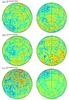 |
Fig. 1 Exaggerated illustration of the aberration and Doppler modulation effects, in orthographic projection, for a velocity v = 260 000 km s-1 = 0.85c (approximately 700 times larger than the expected magnitude) towards the northern pole (indicated by meridians in the upper half of each image on the left). The aberration component of the effect shifts the apparent position of fluctuations towards the velocity direction, while the modulation component enhances the fluctuations in the velocity direction and suppresses them in the anti-velocity direction. |
In this paper, we will present a measurement of β, exploiting the distinctive statistical signatures of the aberration and modulation effects on the high-ℓ CMB temperature anisotropies. In addition to our interest in making an independent measurement of the velocity signature, the effects which velocity generates on the CMB fluctuations provide a source of potential bias or confusion for several aspects of the Planck data. In particular, velocity effects couple to measurements of: primordial “τNL”-type non-Gaussianity, as discussed in Planck Collaboration XXIV (2014); statistical anisotropy of the primordial CMB fluctuations, as discussed in Planck Collaboration XXIII (2014); and gravitational lensing, as discussed in Planck Collaboration XVII (2014). There are also aspects of the Planck analysis for which velocity effects are believed to be negligible, but only if they are present at the expected level. One example is measurement of fNL-type non-Gaussianity, as discussed in Catena et al. (2013). Another example is power spectrum estimation – as discussed above, velocity effects change the angular scale of the acoustic peaks in the CMB power spectrum. Averaged over the full sky this effect is strongly suppressed, as the expansion and contraction of scales on opposing hemispheres cancel out. However the application of a sky mask breaks this cancellation to some extent, and can potentially be important for parameter estimation (Pereira et al. 2010; Catena & Notari 2013). For the 143 and 217 GHz analysis mask used in the fiducial Planck CMB likelihood (Planck Collaboration XV 2014), the average lensing convergence field associated with the aberration effect (on the portion of the sky which is unmasked) has a value which is 13% of its peak value, corresponding to an expected average lensing convergence of β × 0.13 = 1.5 × 10⁻⁴. This will shift the angular scale of the acoustic peaks by the same fraction, which is degenerate with a change in the angular size of the sound horizon at last scattering, θ∗ (Burles & Rappaport 2006). A 1.5 × 10⁻⁴ shift in θ∗ is just under 25% of the Planck uncertainty on this parameter, as reported in Planck Collaboration XVI (2014) – small enough to be neglected, though not dramatically so. This therefore motivates us to test that the observed aberration signal is not significantly larger than expected. With such a confirmation in hand, a logical next step is to correct for these effects by a process of de-boosting the observed temperature (Notari & Quartin 2012; Yoho et al. 2012). Indeed, an analysis of maps corrected for the modulation effect described here is performed in Planck Collaboration XXIII (2014).
Before proceeding to discuss the aberration and modulation effects in more detail, we note
that in addition to the overall peculiar velocity of our Solar System with respect to the
CMB, there is an additional time-dependent velocity effect from the orbit of
Planck (at L2, along with the Earth) about the Sun. This velocity has an
average amplitude of approximately 30 km
s-1, less than one-tenth the size of the primary velocity
effect. The aberration component of the orbital velocity (more commonly referred to in
astronomy as “stellar aberration”) has a maximum amplitude of
 and is corrected for in the satellite
pointing. The modulation effect for the orbital velocity switches signs between each 6-month
survey, and so is suppressed when using multiple surveys to make maps (as we do here, with
the nominal Planck maps, based on a little more than two surveys), and so
we will not consider it further2.
and is corrected for in the satellite
pointing. The modulation effect for the orbital velocity switches signs between each 6-month
survey, and so is suppressed when using multiple surveys to make maps (as we do here, with
the nominal Planck maps, based on a little more than two surveys), and so
we will not consider it further2.
2. Aberration and modulation
Here we will present a more quantitative description of the aberration and modulation effects described above. To begin, note that, by construction, the peculiar velocity, β, measures the velocity of our Solar System barycentre relative to a frame, called the CMB frame, in which the temperature dipole, a1m, vanishes. However, in completely subtracting the dipole, this frame would not coincide with a suitably-defined average CMB frame, in which an observer would expect to see a dipole C1 ~ 10-10, given by the Sachs-Wolfe and integrated Sachs-Wolfe effects (see Zibin & Scott 2008 for discussion of cosmic variance in the CMB monopole and dipole). The velocity difference between these two frames is, however, small, at the level of 1% of our observed v.
If T′ and
 are the CMB temperature
and direction as viewed in the CMB frame, then the temperature in the observed frame is
given by the Lorentz transformation (see, e.g., Challinor
& van Leeuwen 2002; Sollom 2010),
are the CMB temperature
and direction as viewed in the CMB frame, then the temperature in the observed frame is
given by the Lorentz transformation (see, e.g., Challinor
& van Leeuwen 2002; Sollom 2010),
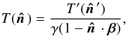 (1)where the observed
direction
(1)where the observed
direction  is given by
 ![Mathematical equation: \begin{equation} \hatn = \frac{\hatn^\prime + [(\gamma - 1)\hatn^\prime\cdot\hat{\vec{v}} + \gamma\beta]\hat{\vec{v}}}{\gamma(1 + \hatn^\prime\cdot\vec{\beta})}, \end{equation}](/articles/aa/full_html/2014/11/aa21556-13/aa21556-13-eq42.png) (2)and γ ≡ (1 − β2)−
1 / 2. Expanding to linear order in β gives
(2)and γ ≡ (1 − β2)−
1 / 2. Expanding to linear order in β gives
 (3)so that we can write
the observed temperature fluctuations as
(3)so that we can write
the observed temperature fluctuations as  (4)Here T0 = (2.7255 ±
0.0006) K is the CMB mean temperature (Fixsen 2009). The first term on the right-hand side of Eq. (4)is the temperature dipole. The remaining term
represents the fluctuations, aberrated by deflection
(4)Here T0 = (2.7255 ±
0.0006) K is the CMB mean temperature (Fixsen 2009). The first term on the right-hand side of Eq. (4)is the temperature dipole. The remaining term
represents the fluctuations, aberrated by deflection  and modulated by the factor
 .
.
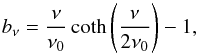
The Planck detectors can be modelled as measuring differential changes in
the CMB intensity at frequency ν given by
![Mathematical equation: \begin{equation} I_\nu(\nu, \hatn) = \frac{2 h \nu^3}{c^2} \frac{1}{ \exp \left[ h \nu / k_{\rm B} T(\hatn) \right] - 1 }\cdot \end{equation}](/articles/aa/full_html/2014/11/aa21556-13/aa21556-13-eq50.png) (5)We can expand the
measured intensity difference according to
(5)We can expand the
measured intensity difference according to 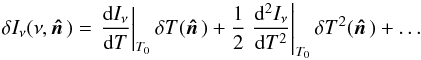 (6)Substituting Eq.
(4)and dropping terms of order
β2
and (δT′)2, we find
(6)Substituting Eq.
(4)and dropping terms of order
β2
and (δT′)2, we find
![Mathematical equation: \begin{equation} \delta I_\nu(\nu,\hatn) = \left.\frac{{\rm d}I_\nu}{{\rm d}T}\right|_{T_0}\! \left[T_0\hatn\cdot\vec{\beta} + \delta T^\prime(\hatn^\prime)(1 + \fnu\hatn\cdot\vec{\beta})\right], \end{equation}](/articles/aa/full_html/2014/11/aa21556-13/aa21556-13-eq53.png) (7)where the frequency
dependent boost factor bν is given by
(7)where the frequency
dependent boost factor bν is given by
 (8)with ν0 ≡
kBT0/h ≃ 57
GHz. Integrated over the Planck bandpasses for the 143
and 217 GHz channels, these effective boost factors are given by b143 = 1.961 ±
0.015, and b217 = 3.071 ± 0.018, where the
uncertainties represent the scatter between the individual detector bandpasses at each
frequency. We will approximate these boost factors simply as b143 = 2 and
b217 =
3, which is sufficiently accurate for the precision of our measurement.
(8)with ν0 ≡
kBT0/h ≃ 57
GHz. Integrated over the Planck bandpasses for the 143
and 217 GHz channels, these effective boost factors are given by b143 = 1.961 ±
0.015, and b217 = 3.071 ± 0.018, where the
uncertainties represent the scatter between the individual detector bandpasses at each
frequency. We will approximate these boost factors simply as b143 = 2 and
b217 =
3, which is sufficiently accurate for the precision of our measurement.
In the mapmaking process, the fluctuations are assumed to satisfy only the linear term in
Eq. (6). Therefore, the inferred temperature
fluctuations will be  (9)Notice that, compared with
the actual fluctuations in Eq. (4), the
modulation term in Eq. (9)has taken on a
peculiar frequency dependence, represented by bν. This has arisen due
to the coupling between the fluctuations and the dipole,
(9)Notice that, compared with
the actual fluctuations in Eq. (4), the
modulation term in Eq. (9)has taken on a
peculiar frequency dependence, represented by bν. This has arisen due
to the coupling between the fluctuations and the dipole,
 , which leads to a
second-order term in the expansion of Eq. (6). Intuitively, the CMB temperature varies from one side of the sky to the other at
the 3 mK level. Therefore so does the calibration factor dIν/
dT, as represented by the second derivative
d2Iν/
dT2. We note that such a
frequency-dependent modulation is not uniquely a velocity effect, but would have arisen in
the presence of any sufficiently large temperature fluctuation. Of course if we measured
, which leads to a
second-order term in the expansion of Eq. (6). Intuitively, the CMB temperature varies from one side of the sky to the other at
the 3 mK level. Therefore so does the calibration factor dIν/
dT, as represented by the second derivative
d2Iν/
dT2. We note that such a
frequency-dependent modulation is not uniquely a velocity effect, but would have arisen in
the presence of any sufficiently large temperature fluctuation. Of course if we measured
 directly
(for example by measuring
directly
(for example by measuring  at a
large number of frequencies), we would measure the true fluctuations, Eq. (4), i.e., we would have a boost factor of
bν
= 1. However, this is not what happens in practice, and hence the
velocity-driven modulation has a spectrum which mixes in a d2Iν/
dT2 dependence.
at a
large number of frequencies), we would measure the true fluctuations, Eq. (4), i.e., we would have a boost factor of
bν
= 1. However, this is not what happens in practice, and hence the
velocity-driven modulation has a spectrum which mixes in a d2Iν/
dT2 dependence.
3. Methodology
The statistical properties of the aberration-induced stretching and compression of the CMB
anisotropies are manifest in “statistically anisotropic” contributions to the covariance
matrix of the CMB, which we can use to reconstruct the velocity vector (Burles & Rappaport 2006; Kosowsky & Kahniashvili 2011; Amendola et al. 2011). To discuss these it will be useful to introduce the
harmonic transform of the peculiar velocity vector, given by
 (10)Here βLM is only non-zero for
dipole modes (with L =
1). Although most of our equations will be written in terms of
βLM, for simplicity of
interpretation we will present results in a specific choice of basis for the three dipole
modes of orthonormal unit vectors, labelled β∥ (along the expected
velocity direction), β× (perpendicular to
β∥ and parallel to the Galactic
plane, near its centre), and the remaining perpendicular mode β⊥.
The directions associated with these modes are plotted in Fig. 2.
(10)Here βLM is only non-zero for
dipole modes (with L =
1). Although most of our equations will be written in terms of
βLM, for simplicity of
interpretation we will present results in a specific choice of basis for the three dipole
modes of orthonormal unit vectors, labelled β∥ (along the expected
velocity direction), β× (perpendicular to
β∥ and parallel to the Galactic
plane, near its centre), and the remaining perpendicular mode β⊥.
The directions associated with these modes are plotted in Fig. 2.
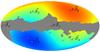 |
Fig. 2 Specific choice for the decomposition of the dipole vector β in
Galactic coordinates. The CMB dipole direction |

In the statistics of the CMB fluctuations, peculiar velocity effects manifest themselves as
a set of off-diagonal contributions to the CMB covariance matrix:
 (11)where
the weight function Wβν
is composed of two parts, related to the aberration and modulation effects, respectively,
(11)where
the weight function Wβν
is composed of two parts, related to the aberration and modulation effects, respectively,
 (12)and the term in large
parentheses is a Wigner 3-j symbol. It should be understood that in all of the
expressions in this section, we take L = 1 for our calculations. We have written the
expressions in more general form to allow easier connection to more general estimators in
the literature. The aberration term, for example, is identical to that found when
considering gravitational lensing of the CMB by large-scale structure (Lewis & Challinor 2006; Planck
Collaboration XVII 2014),
(12)and the term in large
parentheses is a Wigner 3-j symbol. It should be understood that in all of the
expressions in this section, we take L = 1 for our calculations. We have written the
expressions in more general form to allow easier connection to more general estimators in
the literature. The aberration term, for example, is identical to that found when
considering gravitational lensing of the CMB by large-scale structure (Lewis & Challinor 2006; Planck
Collaboration XVII 2014),  (13)while
the modulation term is identical to that produced by an inhomogeneous optical depth to the
last scattering surface (Dvorkin & Smith
2009),
(13)while
the modulation term is identical to that produced by an inhomogeneous optical depth to the
last scattering surface (Dvorkin & Smith
2009),  (14)Note that one might,
in principle, be concerned about order β2 corrections to the covariance matrix,
particularly at high ℓ (see, e.g., Notari
& Quartin 2012). However, these are small, provided that the spectra are
relatively smooth. Although the order β (≃10-3) deflections give large changes to the aℓms for ℓ > 103, the
changes to the overall covariance are small (Chluba
2011), since the deflection effect is coherent over very large scales.
(14)Note that one might,
in principle, be concerned about order β2 corrections to the covariance matrix,
particularly at high ℓ (see, e.g., Notari
& Quartin 2012). However, these are small, provided that the spectra are
relatively smooth. Although the order β (≃10-3) deflections give large changes to the aℓms for ℓ > 103, the
changes to the overall covariance are small (Chluba
2011), since the deflection effect is coherent over very large scales.
The basic effect of these boosting-induced correlations is to couple ℓ modes with ℓ ± 1 modes. They therefore share this property with pure dipolar amplitude modulations studied in the context of primordial statistical anisotropy (see, e.g., Prunet et al. 2005), as well as with dipolar modulations in more general physical parameters (Moss et al. 2011). However, these other cases do not share the frequency dependence of the boosting modulation effect, since they are not accompanied by a temperature dipole.
We measure the peculiar velocity dipole using quadratic estimators, essentially summing
over the covariance matrix of the observed CMB fluctuations, with weights designed to
optimally extract β. A general quadratic estimator
 for βLM is given
by (Hanson & Lewis 2009)
for βLM is given
by (Hanson & Lewis 2009) ![Mathematical equation: \begin{eqnarray} \hat{x\,}_{LM}[\bar{T}] &=& \frac{1 }{2} N_L^{x \betanu} \sum_{\ell_1= \ell_{\rm min}}^{\ell_{\rm max}} \sum_{\ell_2= \ell_{\rm min}}^{\ell_{\rm max}} \sum_{m_1, m_2} (-1)^M \threej{\ell_1}{\ell_2}{L}{m_1}{m_2}{-M} W_{\ell_1 \ell_2 L}^{{x\,}} \nonumber \\ &&\quad \times \left( \bar{T}^{}_{\ell_1 m_1} \bar{T}^{}_{\ell_2 m_2} - \left\langle \bar{T}^{}_{\ell_1 m_1} \bar{T}^{}_{\ell_2 m_2} \right\rangle \right), \label{eqn:qe_block} \end{eqnarray}](/articles/aa/full_html/2014/11/aa21556-13/aa21556-13-eq90.png) (15)where
(15)where
 are a set of inverse-variance filtered temperature multipoles,
 is a weight function
and
is a weight function
and  is a normalization. To study the total boosting effect we use Eq. (12)for the weight function, but we will also use
weight functions designed to extract specifically the aberration and modulation components
of the effect. The ensemble average term ⟨⟩ is taken over signal+noise realizations of the CMB in the absence of
velocity effects. It corrects for the statistical anisotropy induced by effects like beam
asymmetry, masking, and noise inhomogeneity. We evaluate this term using Monte Carlo
simulations of the data, as discussed in Sect. 4.
is a normalization. To study the total boosting effect we use Eq. (12)for the weight function, but we will also use
weight functions designed to extract specifically the aberration and modulation components
of the effect. The ensemble average term ⟨⟩ is taken over signal+noise realizations of the CMB in the absence of
velocity effects. It corrects for the statistical anisotropy induced by effects like beam
asymmetry, masking, and noise inhomogeneity. We evaluate this term using Monte Carlo
simulations of the data, as discussed in Sect. 4.
We use three different quadratic estimators to measure the effects of boosting. The first,
 ,
simply adopts the weight function
,
simply adopts the weight function  , and
provides a minimum-variance estimator of the total peculiar velocity effect. The two
additional estimators,
, and
provides a minimum-variance estimator of the total peculiar velocity effect. The two
additional estimators,  and
and  ,
isolate the aberration and modulation aspects of the peculiar velocity effect, respectively.
This can be useful, as they are qualitatively quite distinct effects, and suffer from
different potential contaminants. The modulation effect, for example, is degenerate with a
dipolar pattern of calibration errors on the sky, while the aberration effect is
indistinguishable from a dipolar pattern of pointing errors.
,
isolate the aberration and modulation aspects of the peculiar velocity effect, respectively.
This can be useful, as they are qualitatively quite distinct effects, and suffer from
different potential contaminants. The modulation effect, for example, is degenerate with a
dipolar pattern of calibration errors on the sky, while the aberration effect is
indistinguishable from a dipolar pattern of pointing errors.
There is a subtlety in the construction of these estimators, due to the fact that the
covariances, described by Wφ and Wτ, are not orthogonal. To
truly isolate the aberration and modulation effects, we form orthogonalized weight matrices
as 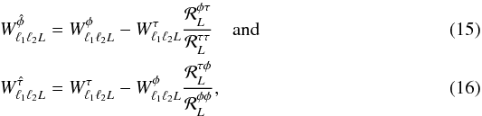 where
the response function ℛ is given
by
where
the response function ℛ is given
by 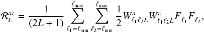 (18)with x,z =
βν,φ,τ.
The construction of these estimators is analogous to the construction of “bias-hardened”
estimators for CMB lensing (Namikawa et al. 2013).
The spectra Fℓ are diagonal
approximations to the inverse variance filter, which takes the sky map
(18)with x,z =
βν,φ,τ.
The construction of these estimators is analogous to the construction of “bias-hardened”
estimators for CMB lensing (Namikawa et al. 2013).
The spectra Fℓ are diagonal
approximations to the inverse variance filter, which takes the sky map
 .
We use the same inverse variance filter as that used for the baseline results in Planck Collaboration XVII (2014), and the approximate
filter functions are also specified there. Note that our
estimator is slightly different from that used in Planck
Collaboration XVII (2014), due to the fact that we have orthogonalized it with
respect to τ.
.
We use the same inverse variance filter as that used for the baseline results in Planck Collaboration XVII (2014), and the approximate
filter functions are also specified there. Note that our
estimator is slightly different from that used in Planck
Collaboration XVII (2014), due to the fact that we have orthogonalized it with
respect to τ.
The normalization
can be approximated analytically as ![Mathematical equation: \begin{equation} N_L^{x \betanu} \simeq \left[ {\cal R}_L^{x \betanu} \right]^{-1}. \label{eqn:nlxbnu} \end{equation}](/articles/aa/full_html/2014/11/aa21556-13/aa21556-13-eq108.png) (19)This approximation does not
account for masking. On a masked sky, with this normalization, we expect to find that
(19)This approximation does not
account for masking. On a masked sky, with this normalization, we expect to find that
 , where
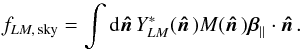 (20)Here
 is the
sky mask used in our analysis. For the fiducial sky mask we use (plotted in Fig. 2, and which leaves approximately 70% of the sky unmasked), taking the dot
product of f1M, sky with our three
basis vectors we find that f∥ , sky = 0.82, f⊥ , sky = 0.17,
and f× , sky = −
0.04. The large effective sky fraction for the β∥
direction reflects the fact that the peaks of the expected velocity dipole are untouched by
the mask, while the small values of fsky for the other components reflects
that fact that the masking procedure does not leak a large amount of the dipole signal in
the β∥ direction into other modes.
is the
sky mask used in our analysis. For the fiducial sky mask we use (plotted in Fig. 2, and which leaves approximately 70% of the sky unmasked), taking the dot
product of f1M, sky with our three
basis vectors we find that f∥ , sky = 0.82, f⊥ , sky = 0.17,
and f× , sky = −
0.04. The large effective sky fraction for the β∥
direction reflects the fact that the peaks of the expected velocity dipole are untouched by
the mask, while the small values of fsky for the other components reflects
that fact that the masking procedure does not leak a large amount of the dipole signal in
the β∥ direction into other modes.
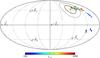 |
Fig. 3 Measured dipole direction |
4. Data and simulations
Given the frequency-dependent nature of the velocity effects we are searching for (at least for the τ component), we will focus for the most part on estimates of β obtained from individual frequency maps, although in Sect. 6 we will also discuss the analysis of component-separated maps obtained from combinations of the entire Planck frequency range. Our analysis procedure is essentially identical to that of Planck Collaboration XVII (2014), and so we only provide a brief review of it here. We use the 143 and 217 GHz Planck maps, which contain the majority of the available CMB signal probed by Planck at the high multipoles required to observe the velocity effects. The 143 GHz map has a noise level that is reasonably well approximated by 45 μK arcmin white noise, while the 217 GHz map has approximately twice as much noise power, with a level of 60 μK arcmin. The beam at 143 GHz is approximately 7′ FWHM, while the 217 GHz beam is 5′ FWHM. This increased angular resolution, as well as the larger size of the τ-type velocity signal at higher frequency, makes 217 GHz slightly more powerful than 143 GHz for detecting velocity effects (the HFI 100 GHz and LFI 70 GHz channels would offer very little additional constraining power). At these noise levels, for 70% sky coverage we Fisher-forecast a 20% measurement of the component β∥ at 217 GHz (or, alternatively, a 5σ detection) or a 25% measurement of β∥ at 143 GHz, consistent with the estimates of Kosowsky & Kahniashvili (2011) and Amendola et al. (2011). As we will see, our actual statistical error bars determined from simulations agree well with these expectations.
The Planck maps are generated at HEALPix (Górski et al. 2005)3Nside =
2048. In the process of mapmaking, time-domain observations are binned
into pixels. This effectively generates a pointing error, given by the distance between the
pixel centre to which each observation is assigned and the true pointing direction at that
time. The pixels at Nside = 2048 have a typical dimension of
 . As this is comparable to the size of the
aberration effect we are looking for, this is a potential source of concern. However, as
discussed in Planck Collaboration XVII (2014), the
beam-convolved CMB is sufficiently smooth on these scales that it is well approximated as a
gradient across each pixel, and the errors accordingly average down with the distribution of
hits in each pixel. For the frequency maps that we use, the rms pixelization error is on the
order of
. As this is comparable to the size of the
aberration effect we are looking for, this is a potential source of concern. However, as
discussed in Planck Collaboration XVII (2014), the
beam-convolved CMB is sufficiently smooth on these scales that it is well approximated as a
gradient across each pixel, and the errors accordingly average down with the distribution of
hits in each pixel. For the frequency maps that we use, the rms pixelization error is on the
order of  , and not coherent over the large dipole
scales which we are interested in, and so we neglect pixelization effects in our
measurement.
, and not coherent over the large dipole
scales which we are interested in, and so we neglect pixelization effects in our
measurement.
We will use several data combinations to measure β. The quadratic estimator of Eq.
(15)has two input “legs”, i.e., the
ℓ1m1 and
ℓ2m2 terms.
Starting from the 143 and 217 GHz maps, there are three distinct ways we may source these
legs: (1) both legs use either the individually filtered 143 GHz or 217 GHz maps, which we
refer to as 143 × 143 and
217 × 217, respectively; (2)
we can use 143 GHz for one leg, and 217 GHz for the other, referred to as 143 × 217; and (3) we can combine both 143 and
217 GHz data in our inverse-variance filtering procedure into a single minimum-variance map,
which is then fed into both legs of the quadratic estimator. We refer to this final
combination schematically as “143+217”. Combinations (2) and (3) mix 143 and 217 GHz data.
When constructing the weight function of Eq. (12)for these combinations we use an effective bν =
2.5. Note that this effective bν is only used to
determine the weight function of the quadratic estimator; errors in the approximation will
make our estimator suboptimal, but will not bias our results. To construct the
 ,
which are the inputs for these quadratic estimators, we use the filtering described in
Appendix A of Planck Collaboration XVII (2014), which
optimally accounts for the Galactic and point source masking (although not for the
inhomogeneity of the instrumental noise level). This filter inverse-variance weights the CMB
fluctuations, and also projects out the 857 GHz Planck map as a dust
template.
,
which are the inputs for these quadratic estimators, we use the filtering described in
Appendix A of Planck Collaboration XVII (2014), which
optimally accounts for the Galactic and point source masking (although not for the
inhomogeneity of the instrumental noise level). This filter inverse-variance weights the CMB
fluctuations, and also projects out the 857 GHz Planck map as a dust
template.
To characterize our estimator and to compute the mean-field term of Eq. (15), we use a large set of Monte Carlo
simulations. These are generated following the same procedure as those described in Planck Collaboration XVII (2014); they incorporate the
asymmetry of the instrumental beam, gravitational lensing effects, and realistic noise
realizations from the FFP6 simulation set described in Planck Collaboration I (2014) and Planck
Collaboration (2013). There is one missing aspect of these simulations which we
discuss briefly here: due to an oversight in their preparation, the gravitational lensing
component of our simulations only included lensing power for lensing modes on scales
L ≥ 2, which
leads to a slight underestimation of our simulation-based error bars for the φ component of the velocity
estimator. The lensing dipole power in the fiducial ΛCDM model is
 ,
which represents an additional source of noise for each mode of β, given by
σφ,lens = 1.2 ×
10-4, or about one tenth the size of the expected signal. The
φ part of the
estimator contributes approximately 46% of the total β estimator weight at 143 GHz, and 35% at 217 GHz. Our measurement errors
without this lensing noise on an individual mode of β are
σβ
≃ 2.5 × 10⁻⁴, while with lensing noise included we would
expect this to increase to
,
which represents an additional source of noise for each mode of β, given by
σφ,lens = 1.2 ×
10-4, or about one tenth the size of the expected signal. The
φ part of the
estimator contributes approximately 46% of the total β estimator weight at 143 GHz, and 35% at 217 GHz. Our measurement errors
without this lensing noise on an individual mode of β are
σβ
≃ 2.5 × 10⁻⁴, while with lensing noise included we would
expect this to increase to 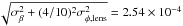 .
This is small enough that we have neglected it for these results (rather than include it by
hand).
.
This is small enough that we have neglected it for these results (rather than include it by
hand).
We generate simulations both with and without peculiar velocity effects, to determine the normalization of our estimator, which, as we will see, is reasonably consistent with the analytical expectation discussed around Eq. (20). All of our main results with frequency maps use 1000 simulations to determine the estimator mean field and variance, while the component separation tests in Sect. 6 use 300 simulations.
5. Results
We present our results visually in Fig. 3, where we
plot the total measured dipole direction  as a function of the maximum temperature multipole ℓmax used as input
to our quadratic estimators. We can see that all four of our 143/217 GHz based estimators
converge towards the expected dipole direction at high ℓmax. At
ℓmax<
100, we recover the significantly preferred direction of Hoftuft et al. (2009), which is identified when searching
for a dipolar modulation of the CMB fluctuations (see Planck
Collaboration XXIII 2014). The τ component of the velocity effect is degenerate with
such a modulation (at least at fixed frequency), and φ gets little weight from
ℓ <
100, so this is an expected result. The significance of this preferred
direction varies as a function of smoothing scale (Hanson
& Lewis 2009; Bennett et al. 2011;
Planck Collaboration XXIII 2014). To minimize
possible contamination of our results by this potential anomaly, from here onward we
restrict the temperature multipoles used in our β estimation to ℓmin = 500. This
cut removes only about 10% of the total number of modes measured by Planck, and so does not
significantly increase our error bars. Note also that we have verified that our error bars
do not shrink significantly for ℓmax> 2000, since almost all of the
modes measured by Planck are at ℓ < 2000.
as a function of the maximum temperature multipole ℓmax used as input
to our quadratic estimators. We can see that all four of our 143/217 GHz based estimators
converge towards the expected dipole direction at high ℓmax. At
ℓmax<
100, we recover the significantly preferred direction of Hoftuft et al. (2009), which is identified when searching
for a dipolar modulation of the CMB fluctuations (see Planck
Collaboration XXIII 2014). The τ component of the velocity effect is degenerate with
such a modulation (at least at fixed frequency), and φ gets little weight from
ℓ <
100, so this is an expected result. The significance of this preferred
direction varies as a function of smoothing scale (Hanson
& Lewis 2009; Bennett et al. 2011;
Planck Collaboration XXIII 2014). To minimize
possible contamination of our results by this potential anomaly, from here onward we
restrict the temperature multipoles used in our β estimation to ℓmin = 500. This
cut removes only about 10% of the total number of modes measured by Planck, and so does not
significantly increase our error bars. Note also that we have verified that our error bars
do not shrink significantly for ℓmax> 2000, since almost all of the
modes measured by Planck are at ℓ < 2000.
There is a clear tendency in Fig. 3 for the measured velocity to point towards the expected direction β∥. At Planck noise levels, we expect a 1σ uncertainty on each component of β of better than 25%. A 25% uncertainty corresponds to an arctan(1 / 4) = 14° constraint on the direction of β. We plot this contour, as well as the corresponding 2σ contour arctan(2 / 4) = 26°. It is apparent that the measured velocity directions are in reasonable agreement with the CMB dipole.
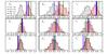 |
Fig. 4 Measurements of β using combinations of the 143
and 217 GHz Planck maps, normalized using Eq. (19)and then divided by the fiducial
amplitude of β = 1.23 ×
10-3. These estimates use ℓmin = 500
and ℓmax =
2000. In addition to the total minimum variance estimate
|
We now proceed to break the measurement of Fig. 3 into
its constituent parts for ℓmax = 2000 (and truncating now at
ℓmin =
500). In Fig. 4 we plot our
quadratic estimates of the three components of β, as well as the decomposition into
aberration and modulation components, for each of our four frequency combinations. The
vertical lines in Fig. 4 give the amplitude estimates
for each component measured from the data, while the coloured and grey histograms give the
distribution of these quantities for the 143 ×
217 estimator, for simulations with and without velocity effects,
respectively (the other estimators are similar). As expected, the velocity effects show up
primarily in β∥; there is little leakage into other
components with our sky mask. For all four estimators, we see that the presence of velocity
along β∥ is strongly preferred over
the null hypothesis. At 143 GHz this signal comes from both
 and
and
 . At 217 GHz it comes
primarily from . Additionally, there is
a somewhat unexpected signal at 217
GHz in the β× direction, again driven
by the τ
component. Given the apparent frequency dependence, foreground contamination seems a
possible candidate for this anomalous signal. We will discuss this possibility further in
the next section.
. At 217 GHz it comes
primarily from . Additionally, there is
a somewhat unexpected signal at 217
GHz in the β× direction, again driven
by the τ
component. Given the apparent frequency dependence, foreground contamination seems a
possible candidate for this anomalous signal. We will discuss this possibility further in
the next section.
In Table 1 we present χ2 values for the
β measurements of Fig. 4 under both the null hypothesis of no velocity effects,
and assuming the expected velocity direction and amplitude. We can see that all of our
measurements are in significant disagreement with the “no velocity” hypothesis. The
probability-to-exceed (PTE) values for the “with velocity” case are much more reasonable.
Under the velocity hypothesis, 217 ×
217 has the lowest PTE, of 11%, driven by the large  .
.
In Table 2 we focus on our measurements of the
velocity amplitude along the expected direction β∥, as well as performing
null tests among our collection of estimates. For this table, we have normalized the
estimators, such that the average of  on boosted simulations
is equal to the input value of 369. For all four of our estimators, we find that this normalization
factor is within 0.5% of that
given by Nxβνf∥
,sky, as is already apparent from the triangles along the
horizontal axis of Fig. 4. We can see here, as
expected, that our estimators have a statistical uncertainty on β∥ of between
20% and 25%. However, several of our null tests,
obtained by taking the differences of pairs of β∥ estimates, fail at the level of
2−3σ. We
take the 143 × 217 GHz estimator
as our fiducial measurement; because it involves the cross-correlation of two maps with
independent noise realizations it should be robust to noise modelling. Null tests against
the individual 143 and 217 GHz estimates are in tension at a level of 2σ for this estimator. We
take this tension as a measure of the systematic differences between these two channels, and
conservatively choose the largest discrepancy with the 143 × 217 GHz estimate, namely 0.31, as our systematic error. We therefore
report a measurement of
on boosted simulations
is equal to the input value of 369. For all four of our estimators, we find that this normalization
factor is within 0.5% of that
given by Nxβνf∥
,sky, as is already apparent from the triangles along the
horizontal axis of Fig. 4. We can see here, as
expected, that our estimators have a statistical uncertainty on β∥ of between
20% and 25%. However, several of our null tests,
obtained by taking the differences of pairs of β∥ estimates, fail at the level of
2−3σ. We
take the 143 × 217 GHz estimator
as our fiducial measurement; because it involves the cross-correlation of two maps with
independent noise realizations it should be robust to noise modelling. Null tests against
the individual 143 and 217 GHz estimates are in tension at a level of 2σ for this estimator. We
take this tension as a measure of the systematic differences between these two channels, and
conservatively choose the largest discrepancy with the 143 × 217 GHz estimate, namely 0.31, as our systematic error. We therefore
report a measurement of  , a
significant confirmation of the expected velocity amplitude.
, a
significant confirmation of the expected velocity amplitude.
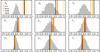 |
Fig. 5 Plot of velocity amplitude estimates, similar to Fig. 4, but using an array of component-separated maps, rather than specific combinations of frequency maps. The production and characterization of these component-separated maps is presented in Planck Collaboration XII (2014). Histograms of simulation results without velocity effects are overplotted in grey for each method; they are all very similar. Vertical coloured bars correspond to the maps indicated in the legend, using the combination of our fiducial galaxy mask (which removes approximately 30% of the sky), as well as the specific mask produced for each component separation method. We see significant departures from the null-hypothesis simulations only in the β∥ direction, as expected. Vertical black lines show the 143 × 217 measurement of Fig. 4. Note the discussion about the subtleties in the normalization of these estimates in Sect. 6. |
6. Potential contaminants
There are several potential sources of contamination for our estimates above which we discuss briefly here, although we have not attempted an exhaustive study of potential contaminants for our estimator.
Galactic Foregrounds: given the simplicity of the
foreground correction we have used (consisting only of masking the sky and projecting out
the Planck 857 GHz map as a crude dust template), foreground contamination
is a clear source of concern. The frequency dependence of the large β× signal seen at
217 GHz, but not at 143 GHz, seems potentially indicative of foreground contamination, as
the Galactic dust power is approximately 10 times larger at 217 than at 143 GHz. To test the
possible magnitude of residual foregrounds, we apply our velocity estimators to the four
component-separated CMB maps of Planck Collaboration XII
(2014), i.e., NILC, SMICA,
SEVEM, and COMMANDER-RULER. Each of these
methods combines the full set of nine Planck frequency maps from 30 to
857 GHz to obtain a best-estimate CMB map. To characterize the scatter and mean field of
each method’s map we use the set of common simulations which each method has been applied
to. These simulations include the effect of the aberration part of the velocity dipole,
although not the frequency-dependent modulation part. For this reason, it is difficult to
accurately assess the normalization of our estimators when applied to these maps,
particularly as they can mix 143 and 217 GHz as a function of scale, and the modulation part
is frequency dependent. We can, however, study them at a qualitative level. The results of
this analysis are shown in Fig. 5. To construct our
β estimator for the component-separated
maps we have used bν = 2.5, assuming that
they contain roughly equal contributions from 143 and 217 GHz. Note that, because the
simulations used to determine the mean fields of the component-separated map included the
aberration part of the velocity effect, it will be absorbed into the mean field if
uncorrected. Because the aberration contribution is frequency independent (so there are no
issues with how the different CMB channels are mixed), and given the good agreement between
our analytical normalization and that measured using simulations for the frequency maps,
when generating Fig. 5 we have subtracted the expected
velocity contribution from the mean field analytically. We see generally good agreement with
the 143 × 217 estimate on which
we have based our measurement of the previous section; there are no obvious discrepancies
with our measurements in the β∥ direction, although
there is a somewhat large scatter between methods for
. In the β×
direction the component-separated map estimates agree well with the 143 × 217 estimator, and do not show the
significant power seen for 217 ×
217, suggesting that the large power that we see there may indeed be
foreground in origin.
Calibration errors: position-dependent calibration errors in our sky maps
are completely degenerate with modulation-type effects (at fixed frequency), and so are very
worrisome as a potential systematic effect. We note that the Planck scan
strategy strongly suppresses map calibration errors with large-scale structure (such as a
dipole, see Planck Collaboration VIII 2014). As the
satellite spins, the detectors mounted in the focal plane inscribe circles on the sky, with
opening angles of between 83°
and 85° (for the 143 and 217 GHz
detectors we use). For a time-dependent calibration error to project cleanly into a dipolar
structure on the sky, it would need to have a periodicity comparable to the spin frequency
of the satellite (1 min-1). Slower fluctuations in the calibration should be
strongly suppressed in the maps. There are calibration errors which are not suppressed by
the scan strategy, however. For example, a nonlinear detector response could couple directly
to the large CMB dipole temperature. Ultimately, because position-dependent calibration
errors are completely degenerate with the τ component of the velocity effect, the only handle
which we have on them for this study is the consistency between
and .
From another viewpoint, the consistency of our measurement with the expected
velocity modulation provides an upper bound on dipolar calibration errors.
Pointing errors: in principle, errors in the pointing are perfectly degenerate with the aberration-type velocity effect in the observed CMB. However the Planck pointing solution has an uncertainty of a few arcseconds rms in both the co- and cross-scan directions (Planck Collaboration VI 2014). The 3′ rms aberrations induced by velocity effects are simply too large to be contaminated by any reasonable pointing errors.
7. Conclusions
From Fig. 3 it is clear that small-scale CMB fluctuations observed in the Planck data provide evidence for velocity effects in the expected direction. This is put on more quantitative footing in Fig. 4 and Table 2, where we see that all four of the 143 and 217 GHz velocity estimators which we have considered show evidence for velocity effects along β∥ at above the 4σ level. Detailed comparison of 143 and 217 GHz data shows some discrepancies, which we have taken as part of a systematic error budget; however, tests with component-separated maps shown in Fig. 5 provide a strong indication that our 217 GHz map has slight residual foreground contamination. The component-separated results are completely consistent with the 143 × 217 estimator which we quote for our fiducial result.
Beyond our peculiar velocity’s impact on the CMB, there have been many studies of related
effects at other wavelengths (e.g., Blake & Wall
2002; Titov et al. 2011; Gibelyou & Huterer 2012). Closely connected are
observational studies which examine the convergence of the clustering dipole (e.g., Itoh et al. 2010; Bilicki
et al. 2011). Indications of non-convergence might be evidence for a super-Hubble
isocurvature mode, which can generate a “tilt” between matter and radiation (Turner 1991), leading to an extremely large-scale bulk
flow. Such a long-wavelength isocurvature mode could also contribute a significant
“intrinsic” component to our observed temperature dipole (Langlois & Piran 1996). However, a peculiar velocity dipole is
expected at the level of  due to structure in standard ΛCDM (see, e.g., Zibin & Scott
2008), which suggests that an intrinsic component, if it exists at all, is
subdominant. In addition, such a bulk flow has been significantly constrained by
Planck studies of the kinetic Sunyaev-Zeldovich effect (Planck Collaboration Int. XIII 2014). In this light, the
observation of aberration at the expected level reported in this paper is fully consistent
with the standard, adiabatic picture of the Universe.
due to structure in standard ΛCDM (see, e.g., Zibin & Scott
2008), which suggests that an intrinsic component, if it exists at all, is
subdominant. In addition, such a bulk flow has been significantly constrained by
Planck studies of the kinetic Sunyaev-Zeldovich effect (Planck Collaboration Int. XIII 2014). In this light, the
observation of aberration at the expected level reported in this paper is fully consistent
with the standard, adiabatic picture of the Universe.
The Copernican revolution taught us to see the Earth as orbiting a stationary Sun. That picture was eventually refined to include Galactic and cosmological motions of the Solar System. Because of the technical challenges, one may have thought it very unlikely to be able to measure (or perhaps even to define) the cosmological motion of the Solar System ... and yet it moves.
Planck (http://www.esa.int/Planck) is a project of the European Space Agency (ESA) with instruments provided by two scientific consortia funded by ESA member states (in particular the lead countries France and Italy), with contributions from NASA (USA) and telescope reflectors provided by a collaboration between ESA and a scientific consortium led and funded by Denmark.
Note that in both stellar and cosmological cases, the aberration is the result of local velocity differences (Eisner 1967; Phipps 1989): in the former case, between Earth’s velocity at different times of the year, and in the latter between the actual and CMB frames.
Acknowledgments
The development of Planck has been supported by: ESA; CNES and CNRS/INSU-IN2P3-INP (France); ASI, CNR, and INAF (Italy); NASA and DoE (USA); STFC and UKSA (UK); CSIC, MICINN, JA, and RES (Spain); Tekes, AoF, and CSC (Finland); DLR and MPG (Germany); CSA (Canada); DTU Space (Denmark); SER/SSO (Switzerland); RCN (Norway); SFI (Ireland); FCT/MCTES (Portugal); and PRACE (EU). A description of the Planck Collaboration and a list of its members, including the technical or scientific activities in which they have been involved, can be found at http://www.sciops.esa.int/index.php?project=planck&page=Planck_Collaboration. Some of the results in this paper have been derived using the HEALPix package. This research used resources of the National Energy Research Scientific Computing Center, which is supported by the Office of Science of the US Department of Energy under Contract No. DE-AC02-05CH11231. We acknowledge support from the Science and Technology Facilities Council [grant number ST/I000976/1].
References
- Amendola, L., Catena, R., Masina, I., et al. 2011, JCAP, 1107, 027 [NASA ADS] [CrossRef] [Google Scholar]
- Bennett, C., Hill, R., Hinshaw, G., et al. 2011, ApJS, 192, 17 [NASA ADS] [CrossRef] [Google Scholar]
- Bilicki, M., Chodorowski, M., Jarrett, T., & Mamon, G. A. 2011, ApJ, 741, 31 [NASA ADS] [CrossRef] [Google Scholar]
- Blake, C., & Wall, J. 2002, Nature, 416, 150 [NASA ADS] [CrossRef] [Google Scholar]
- Burles, S., & Rappaport, S. 2006, ApJ, 641, L1 [NASA ADS] [CrossRef] [Google Scholar]
- Catena, R., Liguori, M., Notari, A., & Renzi, A. 2013, J. Cosmol. Astropart., 9, 36 [NASA ADS] [CrossRef] [Google Scholar]
- Catena, R., & Notari, A. 2013, J. Cosmol. Astropart., 4, 28 [NASA ADS] [CrossRef] [Google Scholar]
- Challinor, A., & van Leeuwen, F. 2002, Phys. Rev., D65, 103001 [Google Scholar]
- Chluba, J. 2011, MNRAS, 415, 3227 [NASA ADS] [CrossRef] [Google Scholar]
- Dvorkin, C., & Smith, K. M. 2009, Phys. Rev., D79, 043003 [NASA ADS] [CrossRef] [Google Scholar]
- Eisner, E. 1967, Am. J. Phys., 35, 817 [NASA ADS] [CrossRef] [Google Scholar]
- Fixsen, D. J. 2009, ApJ, 707, 916 [Google Scholar]
- Fixsen, D., Cheng, E., Gales, J., et al. 1996, ApJ, 473, 576 [NASA ADS] [CrossRef] [Google Scholar]
- Gibelyou, C., & Huterer, D. 2012, MNRAS, 427, 1994 [NASA ADS] [CrossRef] [Google Scholar]
- Górski, K. M., Hivon, E., Banday, A. J., et al. 2005, ApJ, 622, 759 [NASA ADS] [CrossRef] [Google Scholar]
- Hanson, D., & Lewis, A. 2009, Phys. Rev., D80, 3004 [Google Scholar]
- Hinshaw, G., Weiland, J. L., Hill, R. S., et al. 2009, ApJS, 180, 225 [NASA ADS] [CrossRef] [Google Scholar]
- Hoftuft, J., Eriksen, H., Banday, A., et al. 2009, ApJ, 699, 985 [NASA ADS] [CrossRef] [Google Scholar]
- Itoh, Y., Yahata, K., & Takada, M. 2010, Phys. Rev. D, 82, 043530 [NASA ADS] [CrossRef] [Google Scholar]
- Kamionkowski, M., & Knox, L. 2003, Phys. Rev. D, 67, 3001 [Google Scholar]
- Kogut, A., Lineweaver, C., Smoot, G. F., et al. 1993, ApJ, 419, 1 [NASA ADS] [CrossRef] [Google Scholar]
- Kosowsky, A., & Kahniashvili, T. 2011, Phys. Rev. Lett., 106, 1301 [NASA ADS] [CrossRef] [Google Scholar]
- Langlois, D., & Piran, T. 1996, Phys. Rev. D, 53, 2908 [NASA ADS] [CrossRef] [Google Scholar]
- Lewis, A., & Challinor, A. 2006, Phys. Rept., 429, 1 [Google Scholar]
- Moss, A., Scott, D., Zibin, J. P., & Battye, R. 2011, Phys. Rev. D, 84, 3014 [Google Scholar]
- Namikawa, T., Hanson, D., & Takahashi, R. 2013, MNRAS, 431, 609 [NASA ADS] [CrossRef] [Google Scholar]
- Notari, A., & Quartin, M. 2012, JCAP, 1202, 026 [NASA ADS] [CrossRef] [Google Scholar]
- Pereira, T. S., Yoho, A., Stuke, M., & Starkman, G. D. 2010 [arXiv:1009.4937] [Google Scholar]
- Phipps, T. E. 1989, Am. J. Phys., 57, 549 [NASA ADS] [CrossRef] [Google Scholar]
- Planck Collaboration 2013, The Explanatory Supplement to the Planck 2013 results, http://www.sciops.esa.int/wikiSI/planckpla/index.php?title=Main_Page (ESA) [Google Scholar]
- Planck Collaboration I. 2014, A&A, 571, A1 [NASA ADS] [CrossRef] [EDP Sciences] [Google Scholar]
- Planck Collaboration II. 2014, A&A, 571, A2 [NASA ADS] [CrossRef] [EDP Sciences] [Google Scholar]
- Planck Collaboration III. 2014, A&A, 571, A3 [NASA ADS] [CrossRef] [EDP Sciences] [Google Scholar]
- Planck Collaboration IV. 2014, A&A, 571, A4 [NASA ADS] [CrossRef] [EDP Sciences] [Google Scholar]
- Planck Collaboration V. 2014, A&A, 571, A5 [NASA ADS] [CrossRef] [EDP Sciences] [Google Scholar]
- Planck Collaboration VI. 2014, A&A, 571, A6 [NASA ADS] [CrossRef] [EDP Sciences] [Google Scholar]
- Planck Collaboration VII. 2014, A&A, 571, A7 [NASA ADS] [CrossRef] [EDP Sciences] [Google Scholar]
- Planck Collaboration VIII. 2014, A&A, 571, A8 [NASA ADS] [CrossRef] [EDP Sciences] [Google Scholar]
- Planck Collaboration IX. 2014, A&A, 571, A9 [NASA ADS] [CrossRef] [EDP Sciences] [Google Scholar]
- Planck Collaboration X. 2014, A&A, 571, A10 [NASA ADS] [CrossRef] [EDP Sciences] [Google Scholar]
- Planck Collaboration XI. 2014, A&A, 571, A11 [NASA ADS] [CrossRef] [EDP Sciences] [Google Scholar]
- Planck Collaboration XII. 2014, A&A, 571, A12 [NASA ADS] [CrossRef] [EDP Sciences] [Google Scholar]
- Planck Collaboration XIII. 2014, A&A, 571, A13 [NASA ADS] [CrossRef] [EDP Sciences] [Google Scholar]
- Planck Collaboration XIV. 2014, A&A, 571, A14 [NASA ADS] [CrossRef] [EDP Sciences] [Google Scholar]
- Planck Collaboration XV. 2014, A&A, 571, A15 [NASA ADS] [CrossRef] [EDP Sciences] [Google Scholar]
- Planck Collaboration XVI. 2014, A&A, 571, A16 [NASA ADS] [CrossRef] [EDP Sciences] [Google Scholar]
- Planck Collaboration XVII. 2014, A&A, 571, A17 [NASA ADS] [CrossRef] [EDP Sciences] [Google Scholar]
- Planck Collaboration XVIII. 2014, A&A, 571, A18 [NASA ADS] [CrossRef] [EDP Sciences] [Google Scholar]
- Planck Collaboration XIX. 2014, A&A, 571, A19 [NASA ADS] [CrossRef] [EDP Sciences] [Google Scholar]
- Planck Collaboration XX. 2014, A&A, 571, A20 [NASA ADS] [CrossRef] [EDP Sciences] [Google Scholar]
- Planck Collaboration XXI. 2014, A&A, 571, A21 [NASA ADS] [CrossRef] [EDP Sciences] [Google Scholar]
- Planck Collaboration XXII. 2014, A&A, 571, A22 [NASA ADS] [CrossRef] [EDP Sciences] [Google Scholar]
- Planck Collaboration XXIII. 2014, A&A, 571, A23 [NASA ADS] [CrossRef] [EDP Sciences] [MathSciNet] [PubMed] [Google Scholar]
- Planck Collaboration XXIV. 2014, A&A, 571, A24 [NASA ADS] [CrossRef] [EDP Sciences] [Google Scholar]
- Planck Collaboration XXV. 2014, A&A, 571, A25 [NASA ADS] [CrossRef] [EDP Sciences] [Google Scholar]
- Planck Collaboration XXVI. 2014, A&A, 571, A26 [NASA ADS] [CrossRef] [EDP Sciences] [Google Scholar]
- Planck Collaboration XXVII. 2014, A&A, 571, A27 [NASA ADS] [CrossRef] [EDP Sciences] [Google Scholar]
- Planck Collaboration XXVIII. 2014, A&A, 571, A28 [NASA ADS] [CrossRef] [EDP Sciences] [Google Scholar]
- Planck Collaboration XXIX. 2014, A&A, 571, A29 [NASA ADS] [CrossRef] [EDP Sciences] [Google Scholar]
- Planck Collaboration XXX. 2014, A&A, 571, A30 [NASA ADS] [CrossRef] [EDP Sciences] [Google Scholar]
- Planck Collaboration XXXI. 2014, A&A, 571, A31 [NASA ADS] [CrossRef] [EDP Sciences] [Google Scholar]
- Planck Collaboration Int. XIII. 2014, A&A, 561, A97 [NASA ADS] [CrossRef] [EDP Sciences] [Google Scholar]
- Prunet, S., Uzan, J.-P., Bernardeau, F., & Brunier, T. 2005, Phys. Rev. D, 71, 3508 [Google Scholar]
- Sollom, I., 2010, Ph.D. thesis, University of Cambridge, UK [Google Scholar]
- Titov, O., Lambert, S. B., & Gontier, A.-M. 2011, A&A, 529, A91 [NASA ADS] [CrossRef] [EDP Sciences] [Google Scholar]
- Turner, M. S. 1991, Phys. Rev. D, 44, 3737 [NASA ADS] [CrossRef] [Google Scholar]
- Yoho, A., Copi, C. J., Starkman, G. D., & Pereira, T. S. 2012 [arXiv:1211.6756] [Google Scholar]
- Zibin, J. P., & Scott, D. 2008, Phys. Rev. D, 78, 3529 [NASA ADS] [Google Scholar]
All Tables
All Figures
|
Fig. 1 Exaggerated illustration of the aberration and Doppler modulation effects, in orthographic projection, for a velocity v = 260 000 km s-1 = 0.85c (approximately 700 times larger than the expected magnitude) towards the northern pole (indicated by meridians in the upper half of each image on the left). The aberration component of the effect shifts the apparent position of fluctuations towards the velocity direction, while the modulation component enhances the fluctuations in the velocity direction and suppresses them in the anti-velocity direction. |
| In the text | |
|
Fig. 2 Specific choice for the decomposition of the dipole vector β in
Galactic coordinates. The CMB dipole direction |
| In the text | |
|
Fig. 3 Measured dipole direction |
| In the text | |
|
Fig. 4 Measurements of β using combinations of the 143
and 217 GHz Planck maps, normalized using Eq. (19)and then divided by the fiducial
amplitude of β = 1.23 ×
10-3. These estimates use ℓmin = 500
and ℓmax =
2000. In addition to the total minimum variance estimate
|
| In the text | |
|
Fig. 5 Plot of velocity amplitude estimates, similar to Fig. 4, but using an array of component-separated maps, rather than specific combinations of frequency maps. The production and characterization of these component-separated maps is presented in Planck Collaboration XII (2014). Histograms of simulation results without velocity effects are overplotted in grey for each method; they are all very similar. Vertical coloured bars correspond to the maps indicated in the legend, using the combination of our fiducial galaxy mask (which removes approximately 30% of the sky), as well as the specific mask produced for each component separation method. We see significant departures from the null-hypothesis simulations only in the β∥ direction, as expected. Vertical black lines show the 143 × 217 measurement of Fig. 4. Note the discussion about the subtleties in the normalization of these estimates in Sect. 6. |
| In the text | |
Current usage metrics show cumulative count of Article Views (full-text article views including HTML views, PDF and ePub downloads, according to the available data) and Abstracts Views on Vision4Press platform.
Data correspond to usage on the plateform after 2015. The current usage metrics is available 48-96 hours after online publication and is updated daily on week days.
Initial download of the metrics may take a while.