| Issue |
A&A
Volume 566, June 2014
|
|
|---|---|---|
| Article Number | A24 | |
| Number of page(s) | 20 | |
| Section | Extragalactic astronomy | |
| DOI | https://doi.org/10.1051/0004-6361/201322809 | |
| Published online | 02 June 2014 | |
A connection between extremely strong damped Lyman-α systems and Lyman-α emitting galaxies at small impact parameters⋆
1
Institut d’Astrophysique de Paris, CNRS-UPMC, UMR 7095,
98bis Bd Arago,
75014
Paris,
France
e-mail:
This email address is being protected from spambots. You need JavaScript enabled to view it.
2
Departamento de Astronomía, Universidad de Chile,
Casilla 36-D, Santiago, Chile
3
Steward Observatory, University of Arizona,
Tucson
AZ
85721,
USA
4
Astronomy Department, University of Florida,
211 Bryant Space Science Center, PO Box
112055, Gainesville
FL
32611-2055,
USA
5 Institute of Cosmology and Gravitation, University of
Portsmouth, UK
6
Enrico Fermi Institute, University of Chicago,
5640 South Ellis
Avenue, Chicago
IL
60637,
USA
Received:
7
October
2013
Accepted:
13
March
2014
Abstract
We present a study of ~100 high redshift (z ~ 2−4) extremely strong damped Lyman-α systems (ESDLA, with N(H i) ≥ 0.5 × 1022cm-2) detected in quasar spectra from the Baryon Oscillation Spectroscopic Survey (BOSS) of the Sloan Digital Sky Survey (SDSS-III) Data Release 11. We study the neutral hydrogen, metal, and dust content of this elusive population of absorbers and confirm our previous finding that the high column density end of the N(H i) frequency distribution has a relatively shallow slope with power-law index −3.6, similar to what is seen from 21-cm maps in nearby galaxies. The stacked absorption spectrum indicates a typical metallicity ~1/20th solar, similar to the mean metallicity of the overall DLA population. The relatively small velocity extent of the low-ionisation lines suggests that ESDLAs do not arise from large-scale flows of neutral gas. The high column densities involved are in turn more similar to what is seen in DLAs associated with gamma-ray burst afterglows (GRB-DLAs), which are known to occur close to star-forming regions. This indicates that ESDLAs arise from a line of sight passing at very small impact parameters from the host galaxy, as observed in nearby galaxies. This is also supported by simple theoretical considerations and recent high-z hydrodynamical simulations. We strongly substantiate this picture by the first statistical detection of Ly α emission with ⟨LESDLA(Ly α)⟩ ≃ (0.6 ± 0.2) × 1042 erg s-1 in the core of ESDLAs (corresponding to about 0.1 L⋆ at z ~ 2−3), obtained through stacking the fibre spectra (of radius 1 ″ corresponding to ~8 kpc at z ~ 2.5). Statistical errors on the Ly α luminosity are of the order of 0.1 × 1042 erg s-1 but we caution that the measured Ly α luminosity may be overestimated by ~35% due to sky light residuals and/or FUV emission from the quasar host and that we have neglected flux-calibration uncertainties. We estimate a more conservative uncertainty of 0.2 × 1042 erg s-1. The properties of the Ly α line (luminosity distribution, velocity width and velocity offset compared to systemic redshift) are very similar to that of the population of Lyman-α emitting galaxies (LAEs) with LLAE(Ly α) ≥ 1041erg s-1 detected in long-slit spectroscopy or narrow-band imaging surveys. By matching the incidence of ESDLAs with that of the LAEs population, we estimate the high column density gas radius to be about rgas = 2.5 kpc, i.e., significantly smaller than the radius corresponding to the BOSS fibre aperture, making fibre losses likely negligible. Finally, the average measured Ly α luminosity indicates a star-formation rate consistent with the Schmidt-Kennicutt law, SFR (M⊙ yr-1) ≈ 0.6 /fesc, where fesc < 1 is the Ly α escape fraction. Assuming the typical escape fraction of LAEs, fesc ~ 0.3, the Schmidt-Kennicutt law implies a galaxy radius of about rgal ≈ 2.5 kpc. Finally, we note that possible overestimation of the Ly α emission would result in both smaller rgas and rgal. Our results support a close association between LAEs and strong DLA host galaxies.
Key words: quasars: absorption lines / galaxies: high-redshift / galaxies: ISM / galaxies: star formation
Table 2 and Fig. 21 are available in electronic form at http://www.aanda.org
© ESO, 2014
1. Introduction
In the past two decades, astronomers have found several efficient observational strategies to detect and study galaxies in the early Universe. Each strategy targets a subset of the overall population of galaxies, which is then named after the selection technique. Lyman-break galaxies (LBGs, Steidel et al. 1996) are selected in broad-band imaging using colour cuts around the Lyman-limit at 912 Å. Because of this selection, LBGs probe mostly bright massive galaxies with strong stellar continuum (e.g. Steidel et al. 2003; Shapley et al. 2003; Shapley 2011). Since hydrogen recombination following ionisation by young stars produces Ly α emission, this line can also be used to detect star-forming galaxies at high-redshift, where it is conveniently redshifted in the optical domain. Ly α emitting galaxies (more generally called Lyman-α emitters, LAEs, Cowie & Hu 1998; Hu et al. 1998) are detected using narrow-band filters tuned to the wavelength of Ly α (e.g. Rhoads et al. 2000; Ouchi et al. 2008; Ciardullo et al. 2012), long-slit spectroscopy (Rauch et al. 2008; Cassata et al. 2011) or integral field spectroscopy (e.g. Petitjean et al. 1996; Adams et al. 2011). Because their selection is independent of the stellar continuum, these galaxies are often faint in broad-band imaging and likely represent low-mass systems with little dust attenuation (Gawiser et al. 2007). Several studies have attempted to relate these two populations in a single picture by studying how the Ly α emission line properties are related to the galaxy stellar populations (e.g. Lai et al. 2008; Kornei et al. 2010). Additionally, infrared observations together with detections of molecular emission have opened a new and very promising way to study galaxies at high redshift (e.g. Omont et al. 1996; Daddi et al. 2009).
Another and very different technique to detect high-redshift galaxies is based on the absorption they imprint on the spectra of bright background sources, such as quasi-stellar objects (QSOs) or gamma-ray burst (GRB) afterglows. These detections depend only on the gas cross-section and are thus independent of the luminosity of the associated object. Large surveys have demonstrated that Damped Lyman-α systems (DLAs, see Wolfe et al. 2005), characterised by N(H i) ≥ 2 × 1020 cm-2, contain ≥80% of the neutral gas immediately available for star formation (Péroux et al. 2003; Prochaska et al. 2005, 2009; Noterdaeme et al. 2009, 2012b; Zafar et al. 2013).
Constraints on the star-formation activity associated with DLAs can be obtained by measuring the metal abundances in the gas (e.g. Prochaska et al. 2003; Petitjean et al. 2008) and their evolution with cosmic time (e.g. Rafelski et al. 2012). The excitation of different atomic and/or molecular species provides indirect constraints on instantaneous surface star-formation rates (SFRs Wolfe et al. 2003; Srianand et al. 2005; Noterdaeme et al. 2007a,b). Prochaska & Wolfe (1997, 1998) tested a variety of models and concluded that the DLA kinematics, as traced by the profiles of low-ionisation metal absorption lines, could be characteristic of rapidly rotating discs. This interpretation is, however, problematic in the cold dark matter models that predict low rotation speeds (Kauffmann 1996). Alternatively, Ledoux et al. (1998) showed that merging protogalactic clumps can explain the observed profiles, as expected in the now prevailing hierarchical models of galaxy formation (see e.g. Haehnelt et al. 1998). Schaye (2001) proposed that large scale outflows would also give rise to DLAs when seen in absorption against a background QSO and that the outflows would have sufficiently large cross-section to explain a significant fraction of DLAs. It has also been proposed that the fraction of neutral gas in cold streams of gas infalling onto massive galaxies is non-negligible at high redshift, where this is an important mode of galactic growth (e.g. Møller et al. 2013). This gas potentially gives rise to DLAs (Fumagalli et al. 2011) with moderate column densities.
Although the chemical and physical state of the gas in DLAs is relatively well understood, we still know little about the properties (mass, kinematics, stellar content) of the associated galaxy population. Since the total cross-section of DLAs is much larger than that of starlight-emitting regions in observed galaxies, a large fraction of DLAs potentially arises from atomic clouds in the halo or circumgalactic environments, as supported by high-resolution galaxy formation simulations (e.g. Pontzen et al. 2008). Direct detection of galaxies associated with DLAs (hereafter “DLA-galaxies”) is needed to address these issues. This has appeared to be a very difficult task, mainly due to the faintness of the associated galaxies and their unknown location (i.e. impact parameter) with respect to the quasar line of sight. Thankfully, substantial progress has been made in the past few years, owing to improved selection strategies and efficient instrumentation on large telescopes (Bouché et al. 2012; Fynbo et al. 2010, 2011; Noterdaeme et al. 2012a; Péroux et al. 2011). Although still rare, these observations show that it is possible to relate the properties of the gas to star formation activity in the host galaxy (e.g. Krogager et al. 2012). For example, large scale kinematics have recently been invoked to link the absorbing gas with star-forming regions located 10−30 kpc away (e.g. Bouché et al. 2013; Fynbo et al. 2013; Krogager et al. 2013; Kashikawa et al. 2014).
Here, we aim to study the link between star formation and the absorbing gas within or very close to the host galaxy. Our rationale is that this can be achieved by selecting DLAs with very high column densities of neutral hydrogen, which will be closely connected both spatially and physically to star forming regions in galaxies, since a Schmidt-Kennicutt law is expected to apply to quasar absorbers (e.g. Chelouche & Bowen 2010). This idea is also supported by 21-cm maps of nearby galaxies (e.g. Zwaan et al. 2005; Braun 2012) and existing observations of impact parameters for high-z DLA galaxies that decrease with increasing column density (Krogager et al. 2012), an effect which is also seen in simulations (e.g. Pontzen et al. 2008; Yajima et al. 2012; Altay & Theuns 2013).
Until recently, very high column density DLAs, with log N(H i) ~ 22, were very rare occurrences (Guimarães et al. 2012; Noterdaeme et al. 2012a; see also Kulkarni et al. 2012), but the steadily increasing number of quasar spectra obtained by the Sloan Digital Sky Survey (SDSS, York et al. 2000) and more recently by the Baryon Oscillation Spectroscopy Survey (BOSS, Dawson et al. 2013) component of SDSS-III (Eisenstein et al. 2011) opens the possibility to study such a population.
We present our DLA sample in Sect. 2 and its column density distribution in Sect. 3. We then study the metal content of our DLA sample and compare it to the population of DLAs associated with GRB afterglows (Sect. 4). In Sect. 5, we analyse the colour distortions that DLAs induce on their background QSOs. The rest of the paper explores the Ly α emission detected using stacking procedures and discusses the nature of DLA galaxies. Throughout the paper, we use standard ΛCDM cosmology with H0 = 70 km s-1 Mpc-1, ΩΛ = 0.7 and Ωm = 0.3.
2. Sample
DLAs were detected with a fully automatic procedure based on profile recognition using correlation analysis (see Noterdaeme et al. 2009). In Noterdaeme et al. (2012b), we applied this technique to about 65 000 quasar spectra from the SDSS-III BOSS Data Release 9 (Pâris et al. 2012). Here, we extend this search to nearly 140 000 quasar spectra from Data Release 11 that includes DR9 (Ahn et al. 2012) and DR10 (Ahn et al. 2014), to be released together with DR12 in December 2014. The reduction of data obtained with the BOSS spectrograph (Smee et al. 2013) mounted on the SDSS telescope (Gunn et al. 2006) is described in Bolton et al. (2012). Quasar spectra featuring broad absorption lines were rejected from the sample after a systematic visual inspection (see Pâris et al. 2012, 2014). The automatic detection procedure provides the redshift and neutral hydrogen column density for each DLA candidate. Although we focus on systems with N(H i) ≥ 5 × 1021 cm-2, we carefully checked all candidates with column densities down to 0.2 dex below this limit. We paid particular attention to the Lyman series and the low-ionisation metal lines in order to remove possible blends or misidentifications. Whenever we felt it necessary, we refined the redshift measurement based on the low-ionisation metal lines and refitted the DLA profile1. In a few cases, data are of poor quality and there is possibility of mis-indentification or large uncertainty on the N(H i)-measurement. This should affect a small fraction of our sample and would have no effect on any statistical result presented in the paper.
We then selected intervening DLAs with log N(H i) ≥ 21.7 (hereafter called extremely strong DLAs or “ESDLAs”) avoiding proximate DLAs with velocities less than 5000 km s-1 from the QSO as these may be physically associated with the quasar environment. Our sample then consists of 104 intervening ESDLAs with absorption redshifts in the range zabs ≃ 2−4.3 (see Table 2 and Fig. 21). We note that even at Δv < 3000 km s-1, the properties of DLAs are generally consistent with an origin external to the QSO host and may simply sample over-dense environments (Ellison et al. 2010). Our conservative higher velocity cut-off should ensure a very low probability for a given ESDLA to be physically associated with the QSO and increasing this cutoff to 10 000 km s-1 would only reject a further four ESDLAs with almost no consequence on the numbers derived in the paper. Strong proximate DLAs from BOSS are studied in Finley et al. (2013).
3. N(H I)-frequency distribution
Petitjean et al. (1993) showed early that different physical processes shape the N(H i) frequency distribution. Above log N(H i) ~ 20, i.e. the regime probed by DLAs, the gas is neutral and the slope reflects the average projected distribution of the gas in and around high redshift galaxies (e.g. Prochaska et al. 2009). The very high end of this distribution is of particular interest since local processes including molecular hydrogen formation and UV radiation or outflows from star-formation activity will influence its shape (Rahmati et al. 2013; Altay et al. 2013). However, this regime was until recently poorly constrained due to the small cross-section of the high column density gas. The availability of the larger DR9 data-set of DLAs allowed to statistically probe the very high column density end (Noterdaeme et al. 2012b), which we now extend using DR11 data.
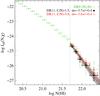 |
Fig. 1 DLA N(H i)-distribution function. The high column density end of the distribution studied here is shown in black for the overall DR11 sample and a subset with higher continuum-to-noise ratio (red). Green points show the results from Noterdaeme et al. (2012b) based on DR9. |
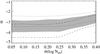 |
Fig. 2 Measured power-law slope as a function of input slope and measurement uncertainty. The different regions (respectively dotted, grey area, dashed) show the 1σ range around the mean value for respectively αi = −3; −3.5 and − 4. |
Figure 1 presents the N(H i) frequency distribution derived from our sample. We confirm our previous result (Noterdaeme et al. 2012b) that the distribution extends to very high column densities (log N(H i) = 22.35) with a moderate power-law slope, although steeper than what is seen at lower column densities (see Prochaska et al. 2014, for a discussion on the shape of the high redshift N(H i)-distribution over the range 1012−1022 cm-2). Including all the lines of sight searched for ESDLAs (with continuum-to-noise ratio2C/N > 1.5), we derive a power-law slope α = −3.7 ± 0.4. Restricting the sample to lines of sight with twice the minimum C/N value (i.e. C/N > 3), we get α = −3.6 ± 0.4. There is a small systematic normalisation offset between the two distributions (resp. −24.51 and −24.46 at log N(H i) = 21.7), but it remains within errors. This indicate little, if any, S/N-dependent bias. If actually present, any bias would indicate slightly lower completeness at low data quality rather than poor identification because the normalisation increases slightly when considering C/N > 3. Indeed, restricting to C/N > 5 does not introduce significant change either in the slope (α = −3.6 ± 0.4) or in the normalisation (−24.43 at log N(H i) = 21.7).
We note that measurement uncertainties combined with limited sample size can in principle introduce a bias in the power-law slope measurement (Koen & Kondlo 2009). To test this, we simulate a DLA population with column density distributions of power-law slopes αi = −3, −3.5, −4, to which we added measurement uncertainties (1σ level ranging from 0.05 to 0.40 dex by step 0.05 dex, see Fig. 2). We reconstruct the resulting “observed” distribution function for 104 ESDLAs randomly selected from this population and repeat this exercise 50 times for each input slope and measurement uncertainty. We find that the slope tends to be shallower with increasing measurement uncertainties (see Fig. 2). While this test remains simplistic, it supports our neglecting systematic errors as the 1σ uncertainty on log N(H i) measured in SDSS spectra is typically less than 0.3 dex (Noterdaeme et al. 2009, see also Fig. 21), although it can be larger in a few cases.
While the large number of quasars discovered by BOSS allows us to constrain for the first time the slope of the N(H i) frequency distribution at the very high column density end, the sample size remains too small to perform statistically sound studies on subsamples (e.g. as a function of the absorber’s redshift). Nonetheless, no strong evolution in the slope of the distribution function is seen in the redshift range z = 2−4. Finally, as noted by Noterdaeme et al. (2012b), the slope of the distribution is close to that derived in nearby galaxies from opacity-corrected 21-cm emission maps (Braun 2012).
4. Absorption properties
4.1. Metal equivalent widths
The equivalent width of metal absorption lines was obtained automatically for each system by locally normalising the quasar continuum around each line of interest and subsequently modelling the absorption lines with a Voigt profile. For non-detections, an upper-limit was derived from the noise around the expected line position, assuming an optically thin regime. Upper-limits were also set for absorptions clearly blended with a line from another system. It is important to note here that most of the lines are saturated even if the apparent optical depth is small because of the low spectral resolution (R ~ 2000). Although the EWs of absorption systems can provide some statistical indication of their metallicity and/or velocity widths, it is necessary to measure EWs from optically thin lines to accurately derive the metallicity. The S/N of SDSS spectra generally does not allow meaningful metallicity estimates for individual systems.
In order to derive the typical metal content of ESDLAs and avoid blending with Ly α forest lines, we produced an average absorption spectrum by stacking the portion of the normalised spectra redwards the Ly α forest. To do this, we first shifted the spectra to the DLA-rest frame and rebinned the data onto a common grid, keeping the same pixel size (constant in velocity space) as the original data. For each pixel i, the stacked spectrum is taken as the median of the normalised fluxes measured at λi. Note that we do not apply any weighting, which means that each DLA contributes equally to the stacked, as long as it covers the considered wavelength. Residual broad-band imperfections in the normalisation (resulting from combining imperfections in individual spectra in different wavelength ranges) were then corrected by re-normalising the stacked spectrum using a median-smoothing filter to get the pseudo-continuum. The resulting stacked spectrum reaches a signal-to-noise ratio (S/N) per pixel of about 50 (see Fig. 3), which sets the typical 1σ detection limit to about 0.02 Å for an unresolved line at the BOSS spectral resolution and sampling.
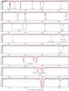 |
Fig. 3 Median ESDLA absorption spectrum redwards of the QSO Ly-α emission. The grey line shows the fraction of the total sample contributing to the stacked spectrum at a given wavelength. |
Thirty-eight absorption features are detected between 1300 and 2900 Å (rest-frame). These arise mostly from low-ionisation species (e.g. Fe ii, Si ii, Zn ii, Cr ii, Mg i) but also from high-ionisation species (Si iv, C iv). Weak lines such as Fe ii λλ2249,2260 are clearly detected even though they are well below the detection limit for any individual spectrum. Fe ii λ1611, Ni ii λ1454 and the Ti ii λ1910 doublet are also possibly detected, but at less than the 3σ level. We proceed to measure the average equivalent widths of the different absorption features through Gaussian fitting (see Table 1). Interestingly, these are the same lines that are detected in a stack by Khare et al. (2012) using the whole DLA catalogue by Noterdaeme et al. (2009), which reaches much higher S/N. However, the equivalent widths of weak lines are found ten times higher here than in Khare et al. (2012), consistent with the ten times higher H i column densities. This already indicates that the abundances in ESDLAs should not be significantly different from that of the overall DLA population.
Similarly, in Fig. 4, we compare the distribution of Si ii λ1526 equivalent widths measured in individual ESDLAs to that of a sample drawn from SDSS without any criterion on N(H i) (Jorgenson et al. 2013). There is a deficit of small EWs (≲0.6 Å) in ESDLAs compared to the overall DLA population, with an almost zero probability that this is due to chance coincidence. We note that this is not due to incompleteness at low EWs, as only one system has Si ii λ1526 undetected at 3σ (a weak line in a low S/N spectrum). This suggests that ESDLAs do not reach drastically lower abundances than the rest of the DLA population.
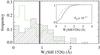 |
Fig. 4 Distributions of the Si ii λ1526 equivalent width measured in ESDLAs (hashed black histogram) and in a sample representative of the overall population of DLAs (green Jorgenson et al. 2013). The vertical line corresponds to the equivalent width (the 1 σ error is represented by the grey area) measured in the stacked ESDLA spectrum. The inset shows the corresponding cumulative distributions (solid black: ESDLAs, dashed green: Jorgenson et al. 2013). |
Equivalent widths of metal absorption lines.
4.2. Abundances and depletion
The column density of different species can then be obtained under the optically thin assumption. This assumption is only valid for weak lines. We again caution that even very strong lines in the optically thick regime appear non-saturated at the BOSS spectral resolution. We estimate column densities for Ni ii, Mn ii, Ti ii, Mg i and Cr ii. Zn ii has two transitions at 2026 and 2062 Å that are unfortunately badly blended with Mg i λ2026 and Cr ii λ2062 (see York et al. 2006, for a discussion about these lines blending at SDSS spectral resolution).
We use the Mg i λ2852 line to derive the Mg i column density and estimate its contribution to the 2026 Å feature, which we find amounts to about 10% of the total equivalent width. Removing this contribution, we then get log N(Zn ii) = 13.1 ± 0.1. We note that if Mg i λ2852 exceeds the optically thin regime, its column density and hence the contribution of Mg i to the 2026 Å feature could be underestimated. In any case, Zn ii λ2026 provides the dominant component in this absorption. Repeating the same procedure with Cr ii and the 2062 Å feature, we measure log N(Zn ii) = 12.7 ± 0.6. The error here is larger because the equivalent width of this absorption is mainly due to Cr ii.
Since several Fe ii and Si ii lines spanning a wide range in oscillator strengths are available, it is possible to construct the curve-of-growth for these species and derive both the column density and the effective Doppler parameter (Fig. 5). The column density is well constrained by weak lines but for stronger lines the equivalent widths reflect mostly the velocity extension of the profile (e.g. Nestor et al. 2003; Ellison 2006). We thus get the average log N(Si ii) = 16.0 ± 0.1 and log N(Fe ii) = 15.5 ± 0.1.
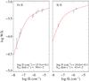 |
Fig. 5 Curve-of-growth for Fe ii (left) and Si ii (right) in the stacked spectrum. |
Using the Zn ii column density derived from the stacked spectrum and the median
hydrogen column density in our sample of ESDLAs, log N(H i) = 21.8,
we estimate the average ESDLA metallicity to be about 1/20th solar. This is consistent
with the mean metallicity found for the overall DLA population across the same redshift
range (⟨Z⟩ = (−0.22 ± 0.03)
z − (0.65 ± 0.09), Rafelski et al. 2012). We observe that iron is depleted by about a factor of
three to four compared to zinc, which is slightly higher than the mean for the overall DLA
population. Figure 6 shows the abundance relative to
that of zinc for iron and other species. As with most DLAs, such an abundance pattern is
similar to the mean Halo abundance pattern of the Galaxy. However, we note that the Small
Magellanic Cloud also has a “Halo-like” depletion pattern (Welty et al. 1997), although it is a gas-rich dwarf galaxy. It is
therefore hazardous to rely only on the depletion pattern to derive information about the
physical origin of the gas, the depletion being more dictated by the metallicity than by
the location of the gas in the galaxy. The dust-to-metal ratio measured following De Cia et al. (2013),
 , is similar to that measured in
DLAs associated with long-duration GRB afterglows (GRB-DLAs).
, is similar to that measured in
DLAs associated with long-duration GRB afterglows (GRB-DLAs).
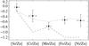 |
Fig. 6 Relative abundance pattern derived from measurements in the stacked absorption spectrum. The dotted (respectively dashed) line shows the typical patterns found in the Halo (respectively warm disc) of the Galaxy (see Welty et al. 1999). |
4.3. Velocity extent
The effective Doppler parameters that we derive independently from the curve-of-growth of Fe ii and Si ii (Fig. 5) are consistent with a single value of beff ~ 40 km s-1, which reflects the absorption line kinematics. Deconvolving the line width from the SDSS spectral profile would be uncertain because of the insufficient SDSS resolution and smoothing resulting from redshift uncertainties when co-adding the spectra. Before comparing our results with previous studies, we note that DLA kinematics are more commonly quantified by their velocity width, Δv, defined as the velocity interval comprising 5−95% of the line optical depth (see Prochaska & Wolfe 1997).
We empirically derive the relation between beff and Δv by applying a curve-of-growth analysis based on Si ii and/or Fe ii equivalent widths measured for systems observed at high spectral resolution, for which Δv is measured accurately (Ledoux et al. 2006). We derive Δv = 2.21 beff + 0.02 beff2 (Fig. 7), which departs from the linear theoretical relation in the Gaussian regime, Δv = 2.33 b, at large values. Interestingly, this could indicate that satellite components increase Δv while not changing much the curve-of-growth (which is derived from integrated equivalent widths). In this view, beff could be an alternative method to quantify absorption-line kinematics, being less sensitive to satellite components than Δv and applicable to data with any spectral resolution as soon as lines with a range of oscillator strengths are covered. Our method also removes the degeneracy between column density and kinematics which could affect studies based on single line equivalent width (e.g. Prochaska et al. 2008). Using this relation, the beff value derived above translates to Δv ≃ 120 km s-1 for the ESDLAs studied here. The mean velocity width of ESDLAs is again consistent with what is seen in the overall DLA population and agrees well with the linear relation between metallicity and velocity extent (Ledoux et al. 2006), within errors.
We emphasise that the mean abundances and depletion factors in ESDLAs are typical of the overall DLA population at this redshift. This suggests that ESDLAs probe the same underlying population of galaxies (i.e. same chemical enrichment history) as most DLAs and that the higher integrated column densities observed along the lines of sight (metal and neutral hydrogen) are a consequence of the hypothesised small impact parameter. The small average velocity extent (~120 km s-1) suggests that ESDLAs do not arise in distant gas ejected from or falling into the host galaxy, contrary to what has been invoked for DLA galaxies with large impact parameters (e.g. Bouché et al. 2013; Krogager et al. 2013).
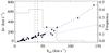 |
Fig. 7 Velocity width, Δv measured by Ledoux et al. (2006) from VLT/UVES spectra as a function of the effective Doppler parameter derived from the equivalent widths of Fe ii and/or Si ii lines. As expected, the theoretical relation for a single unsaturated component, Δv = 2.33b (dotted line), encompasses the data. The dashed line shows the empirical fitted relation Δv = 2.21 beff + 0.02 beff2. The histogram shows the distribution of beff measured in the sample of Ledoux et al. (2006), with the scale on the right axis. The vertical dashed lines mark the values independently found in ESDLAs from Si ii and Fe ii. |
4.4. Note on molecules
According to models by Schaye (2004), the high column density gas collapses into cold and molecular gas (see also Schaye 2001) and eventually forms stars. We therefore anticipate the presence of H2 in high column density systems. In the disc of the Milky Way, the molecular fraction increases sharply beyond log N(H) > 20.7 (Savage et al. 1977). High-latitude Galactic lines of sight show a similar transition (Gillmon et al. 2006), as do those towards the Magellanic Clouds, albeit at higher column densities (log N(H) = 21.3 and 22 for the LMC and SMC, respectively; Tumlinson et al. 2002). However, while there is a possible dependence on the H2 fraction with N(H i) in high-z DLAs, a sharp transition has not yet been observed (Ledoux et al. 2003; Noterdaeme et al. 2008). This is likely due to the very small cross-sections of clouds with large N(H2) (Zwaan & Prochaska 2006) as well as induced extinction. In addition, the transition could occur at higher H i column densities than probed to date. Our sample is therefore a unique opportunity to identify the transition. Although the BOSS spectral resolution and S/N are far too poor to allow for detecting typical H2 lines, it is nonetheless possible to detect H2 if the column density is high enough to produce damping wings. About 20 DR9 ESDLAs from our sample are among the ~10 000 DLAs that Balashev et al. (2014) inspected for very strong H2 systems. Two of them (towards SDSS J004349−025401 and SDSS J084312+022117J) belong to their sample of 23 confident strong H2 systems (with log N(H2) ≳ 19). Among the remaining ESDLAs, the log N(H i) ~ 22 DLA detected toward J 0816+1446 has been observed with UVES and presents H2 lines with N(H2) ~ 5 × 1018 cm-2 (Guimarães et al. 2012). Finally, although it is not in SDSS and hence not part of our sample, the well known H2-bearing DLA toward HE 0027−1836 with N(H2) ~ 2−3 × 10¹⁷ (Noterdaeme et al. 2007a; Rahmani et al. 2013) and log N(H i) = 21.75 also classifies as an ESDLA according to our definition. Molecular hydrogen may be conspicuous in ESDLAs, but observations at higher spectral resolution would be required to investigate the overall sample.
4.5. High-ionisation species
Analysing the Ly α forest of a stacked spectrum is challenging because of uncertainties in the continuum placement and random blending with intervening H i lines (Pieri et al. 2010). Furthermore, because of the different DLA absorption redshifts, only a fraction of the sample contributes to a given rest wavelength in the stacked spectra. Although the O vi doublet is always located in the forest, these transitions are useful to probe hot gas that is potentially related to galactic outflows originating from star-formation activity. Thanks to the small separation between the two lines of the O vi doublet, the above-mentionned difficulties are mostly avoided for this species. We measured rest equivalent widths of 0.44±0.22 and 0.27±0.15 for O vi λ1031 and 1037 respectively from the corresponding portion of the normalised stacked spectrum in Fig. 8. Two points do not allow any consistency check when building a curve-of-growth (that has two parameters), but it is interesting to note that these equivalent widths indicate a column density of about log N(O vi) ~ 14.8 and beff ~ 80 km s-1. The effective Doppler parameter is larger than what is observed for low-ionisation metal lines and indicates a velocity extent of Δv ~300 km s-1 (see Fig. 7). This is among the high values seen in DLAs (Fox et al. 2007), while the O vi column density and metallicity of the neutral gas match the metallicity−N(O vi) correlation presented by these authors. We caution however that these values are indicative only, due to the large error on the O vi EWs. This may indicate that outflows of hot gas (best seen when the line of sight has small impact parameters) could be present. Indeed, Fox et al. (2007) demonstrated that the O vi phase should be hot (>105 K) and collisionally ionised with a baryonic content of at least of similar order as that in the H i phase. However, we caution again that the measurement of Δv is highly uncertain here since O vi λ1037 is blended with C ii λ1036 and O i λ1040, in addition to the Ly α forest. Furthermore, the product of oscillator strengths and wavelengths of the two lines differ only by a factor of two.
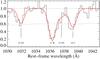 |
Fig. 8 Portion of the normalised stacked spectrum around the O vi doublet. |
4.6. Comparison with GRB-DLAs
In this Section, we compare the ESDLAs properties with those of GRB-DLAs in the same redshift range, z = 2−4. We use the GRB-DLA measurements from Fynbo et al. (2009) with additional values from de Ugarte Postigo et al. (2012). Since GRBs originate from the collapse of massive stars (Bloom et al. 1999), they are expected to occur in star-forming regions. A large fraction of GRB-DLAs have high N(H i) values (e.g. Prochaska et al. 2007; Fynbo et al. 2009), and we concentrate only on the high end of the QSO-DLAs and GRB-DLAs N(H i) distributions (Fig. 9). The distribution for GRB-DLAs is flatter than that for QSO-DLAs and extends up to higher N(H i) values. Interestingly, in most cases, the gas that gives rise to GRB-DLAs is not directly associated with the dying star, but is instead located further away in the host galaxy (e.g. Vreeswijk et al. 2007). This implies that the difference between the two distributions is not related to the properties of the immediate GRB environment but rather related to biases in the GRB sample and inclination effects (Fynbo et al. 2009): since QSOs randomly probe the intervening gas, the corresponding distribution reflects the average gas cross-section at different column densities and includes geometrical effects due to the galaxy inclination. In turn, GRB-DLAs uniformly probe their host galaxy, regardless of their inclination. In other words, face on discs would have a higher probability to appear in QSO surveys compared to edge-on discs, while this should not be the case for GRBs.
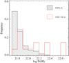 |
Fig. 9 H i column density distribution for our intervening QSO-DLAs with N(H i) ≥ 5 × 1022cm-2 (hashed histogram) compared to that of associated GRB-DLAs (red unfilled histogram, Fynbo et al. 2009; de Ugarte Postigo et al. 2012). |
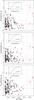 |
Fig. 10 Rest-frame equivalent widths of metal lines as a function of log N(H i). Black are ESDLAs, red are GRB-DLAs from Fynbo et al. (2009) and de Ugarte Postigo et al. (2012). The open/filled squares at log N(H i) = 22.8 correspond to EW in the GRB-DLA 080607 measured at R = 400 and R = 1200 respectively. The horizontal dashed lines correspond to the average EWs measured from the stacked spectrum. |
We compare the equivalent widths of three metal lines for ESDLAs and GRB-DLAs (Fig. 10). We use Si ii λ1526, Fe ii λ1608 and Al ii λ1670 which are generally located in a clean portion of the spectra, redwards of the QSO Ly α emission and bluewards of sky emission lines. The range of Si ii and Al ii equivalent widths decreases with increasing N(H i) for ESDLAs. Conversely, EWs appear to increase at large N(H i) for GRB-DLAs, but this is mostly due to three GRB-DLAs that have column densities in a regime still unprobed by ESDLAs (log N(H i) > 22.5). These also correspond to dark GRBs. If we restrict the comparison to systems with column densities below log N(H i) = 22.5, then the distributions of metal EWs for GRB-DLAs and ESDLAs are very similar, as the Kolmogorov-Smirnov tests indicates. Dust biasing could account for the decrease in the EW upper bound with increasing N(H i), since the extinction increases linearly with the metal column density (Vladilo & Péroux 2005). In this case, the dependence on N(H i) arises indirectly from the fact that the EWs may more represent the velocity extent than the column density, and that this velocity extent increases with metallicity (Ledoux et al. 2006). In other words, systems with both high EW and high-N(H i) are therefore likely to have large metal column densities and hence produce more extinction. However, as we will see in the next section, the average extinction per H atom appears to be relatively small. Another explanation is that at the highest column densities, the line of sight passes closer to the inner region of the host galaxy, where the dispersion in velocity could be less important. It is also possible that, because both high-N(H i) systems and high EWs are uncommon, systems with these two characteristics are simply rarer and would require higher statistics to be represented in the figure.
It is possible that such a decrease in the range of EW does not apply for Fe ii λ1608. This could be due the fact that this line is weaker, and therefore its equivalent width is less dominated by kinematics and more indicative of the column density. If so, the above explanation involving lower kinematics at higher N(H i) would be preferred. In addition, the decrease of Wr(Si ii) and Wr(Al ii) is mostly seen from the upper boundary, while the minimum EW for a given N(HI) bin seems rather to increase with N(H i). This is expected if the metallicity does not depends on N(H i), as the column density contributes more significantly for small EWs. We note that, because GRB DLAs are generally observed at even lower spectral resolution, Fe ii λ1611 and Fe ii⋆λ1612 also contribute to the equivalent width measured for Fe ii λ1608. Excited iron, Fe ii⋆, which is absent in QSO-DLAs, is generally enhanced in GRB-DLAs because of strong excitation from the burst itself. In the case of GRB 080607, de Ugarte Postigo et al. (2012) quote an Fe ii EW measurement based on the R = 400 spectrum from Prochaska et al. (2009) that surprisingly appears significantly higher than the Si ii λ1526 EW, which is an isolated line. The equivalent width measured from their R = 1200 spectrum avoids contamination. As a result, the Fe ii λ1608 EW is significantly lower and more consistent with Si ii λ1526 and Al ii λ1670 (see Fig. 10). The quoted Fe ii λ1608 equivalent widths in GRB-DLAs are thus probably overestimated.
5. Induced colour distortions of the background QSO light.
In this section, we investigate whether the presence of an ESDLA has an effect on the background quasar colour. The top panels of Figs. 11 and 12 represent respectively the (g − r) and (i − z) colours of the quasars as a function of their redshift.
5.1. Ly α absorption
The g − r values for QSOs with foreground ESDLAs are systematically higher than the median colour for the BOSS DR11 QSO population at a given redshift (⟨g − r⟩z, blue line in the figure). This trend is better seen in the distribution of the colour excess Δ(g − r) = (g − r) − ⟨g − r⟩z in the bottom panel, which indicates a systematic difference of about 0.2 mag between the two populations, with an almost zero probability that this is due to chance coincidence. The presence of a damped Ly α absorption can explain the 0.2 mag difference, because the centroid often falls in the g-band. Even when it does not, the extended wings of the absorption profile also affect this band.
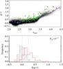 |
Fig. 11 Top: (g − r) colour of the background QSOs as a function of redshift. The black points represent the DR11 QSO sample. QSOs with foreground ESDLA that have a Ly α centroid that falls in the u, g, and r-band are represented by purple, green and red points respectively. The blue line shows the change in the median colour of the overall QSO sample as a function of redshift. Bottom: normalised distributions of colour excess Δ(g − r) = (g − r) − ⟨g − r⟩z for the DR11 QSO sample (black hashed histogram) and the QSO with foreground ESDLAs (red unfilled histogram). The vertical lines mark the medians of the two distributions. |
5.2. Dust extinction
Potential continuum absorption by dust must be investigated at wavelength ranges unaffected by Lyman absorption lines, i.e., the i and z bands. The colour excess is hard to see directly in the (i − z) vs. zQSO plot (Fig. 12), but produces a 0.02 mag difference in the median of the two distributions in the bottom panel. The Kolmogorov-Smirnov test indicates a 20% probability that the two samples are drawn from the same parent distribution.
In order to quantify the reddening effect of intervening ESDLAs on the QSO light, we apply the technique described in Srianand et al. (2008) and Noterdaeme et al. (2010). We match each spectrum with a QSO composite spectrum from Vanden Berk et al. (2001) redshifted to the same zQSO and reddened by a SMC-extinction law at zabs. As for most QSO absorbers (York et al. 2006), this is the preferred extinction law for all but one ESDLA, (towards J 104054+250709) which is best fitted with a LMC-extinction law featuring a 2175-Å UV bump. In the fitting process, we ignore the emission line regions as well as wavelengths bluewards of the QSO Ly α emission. For each QSO with intervening ESDLA in our sample, we repeat the same procedure on a control sample drawn from the same original DR11 QSO sample that we searched for DLAs with an emission redshift close to that of the ESDLA-bearing QSO. We restrict the redshift difference to Δz = 0.001, yielding a typical control sample size of over 100 QSO spectra. For about 25% of the systems we needed to increase this range to obtain at least 50 QSOs for the control sample. The maximum redshift interval in the sample is then Δz = 0.04, which is certainly still small enough to avoid any redshift-dependent differences in the QSO colours. An example of the fitting is shown in Fig. 13.
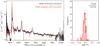 |
Fig. 13 Left: ESDLA BOSS spectrum (black) with the SDSS composite spectrum (grey) reddened by the SMC extinction-law at zabs(red) with E(B − V) = 0.02. The orange segments indicate the regions used for the fit. Right: distribution of E(B − V)-values for the corresponding control sample. In this example, the “zero-point” (respectively dispersion) of the distribution is −0.03 (respectively 0.044). The value retained for the DLA here is thus E(B − V) = 0.05 ± 0.05. |
We measure E(B − V) by subtracting the median of each control sample (our “zero-point”). The control sample dispersion provides the total error on E(B − V) due to fitting uncertainties and intrinsic shape variations. We note that although unrelated absorbers could contribute to the measured reddening in individual ESDLAs, this has no consequence on our statistical result as the control sample is affected the same way. The distribution of E(B − V) is shown in Fig. 14, and is well modelled by a Gaussian centred at E(B − V) = 0.025. The dispersion around the mean is 0.05 mag, matching the mean error on E(B − V), shown as a horizontal error bar. While it is hard to conclusively detect reddening in any individual ESDLA, on average these systems present a small but statistically significant reddening ⟨E(B − V)⟩ ≈ 0.02−0.03, which explains the typical 0.02 mag (i − z) excess measured above.
This corresponds to a specific extinction of the order of AV/N(H i) ~ 10-23 mag cm2, which is similar3 to the median value for the overall (log N(H i) ≥ 20.3) DLA population (Vladilo et al. 2008).
Next we divide our sample into two subsamples with Si ii λ1526 rest-frame equivalent width above and below 0.8 Å. The reddening is statistically stronger in systems with higher Wr(Si iiλ1526), as observed by Khare et al. (2012) for the overall population of DLAs.
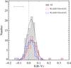 |
Fig. 14 Distribution of E(B − V) values (full sample as hashed histogram, subsample with Wr(Si iiλ1526) above (respectively below) 0.8 Å in red (respectively blue) unfilled histogram), fitted with Gaussian functions. The horizontal error bar in the upper left corner indicates the typical error on E(B − V), obtained from the standard deviation of the values in each control sample. |
6. Lyman α emission from the host galaxy
The background QSO light is completely absorbed at the position of the DLA trough, enabling us to search for Ly α emission from star-formation activity in the vicinity of the neutral gas (see e.g. Rahmani et al. 2010). However, searches for DLA galaxy counterparts based on Ly α emission have resulted mostly in non-detections (e.g. Lowenthal et al. 1995; Møller et al. 2004, as well as numerous unpublished searches). Indeed, because of their cross-section selection, DLAs should arise mostly from galaxies with low star-formation rates (e.g. Cen 2012). The impact parameters can also be larger than the fibre radius, which means that the Ly α emission will not necessarily be detected in the quasar spectrum (such an example is shown in Fynbo et al. 2011; Krogager et al. 2013), although simulations indicate that the impact parameters should be of the order of a few kpc on average (Pontzen et al. 2008; Rahmati & Schaye 2014). Even in cases where oxygen or Balmer emission lines are detected, the Ly α escape fraction can be far from unity, putting the line flux well below the detection threshold. Finally, resonant scattering widens the Ly α line far beyond the virial velocity of the star-forming region. The Ly α line can therefore be spread over the whole DLA core, making it difficult to distinguish the emission from residuals in the zero-flux level. This, together with fibre losses, explains in part why interpreting the residual flux in a stacked DLA spectrum can be challenging (Rahmani et al. 2010; Rauch & Haehnelt 2011).
Extremely strong DLAs allow us to avoid most of the observational obstacles. If very strong column densities truly arise from gas located within a galaxy, then we expect that the light from the galaxy will fall well within the radius of the BOSS fibre (r = 1″ or equivalently, ~8 kpc at z ~ 2.5). Furthermore, the light from the background quasar is completely absorbed across more than 10 Å (rest-frame) for log N(H i) ≥ 21.7, isolating any possible Ly α emission from the wings of the damped profile.
6.1. Stacking procedure
In order to detect faint Ly α emission, we stack quasar spectra in the DLA rest-frame, following the technique described in Rahmani et al. (2010). We restrict our sample to ESDLAs with 2 < zabs < 3.56 to ensure that the expected Ly α emission always falls on the blue CCD. We thereby avoid both the very blue end of the spectrum and the region that overlaps with the red CCD, where spurious spikes are frequently seen. We also exclude the ESDLA toward J1135−0010, for which strong Ly α emission is detected (see Fig. 15)4 and a few systems that have very noisy spectra (C/N< 2) where zabs and N(H i)-measurements are highly uncertain.
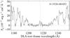 |
Fig. 15 Portion of the BOSS spectrum of SDSS J 113520−001053 in which the double peaked Ly α emission is clearly seen in the DLA trough. |
Our sample for stacking includes 95 flux-calibrated spectra. Each spectrum is shifted to the DLA-rest frame and then rebined to a common grid with the same velocity-constant pixel size as the original BOSS data, conserving the flux per unit wavelength interval. We next convert each spectrum into luminosity per unit wavelength using the luminosity distance at the DLA’s redshift. We produce an average composite spectra using: (i) median; (ii) mean with iterative 3σ rejection of deviant values (“3σ-clipped mean”); and (iii) weighted mean. The latter is produced by weighting each spectrum (in luminosity units) by the squared inverse of the corresponding error (σdark in Table 2).
Figure 16 shows the results of stacking with the three different averaging methods. The Ly α emission appears clearly in the three composite spectra as positive flux in the central pixels. We overplot the scaled LBG composite from Shapley et al. (2003) for comparison.
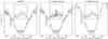 |
Fig. 16 Results from spectral stacking. From left to right, the stacked spectrum corresponds to the median values, 3σ-clipped mean and weighted mean. The long red segment shows the DLA core region over which τ > 6 for log N(H i) ≥ 21.7, ensuring no residual flux from the quasar. This region is highlighted in the inset panels. The short red segment (inner tick marks) indicates the 1000 km s-1 central region over which the Ly α luminosity is integrated. The green spectrum is the composite Lyman-break galaxy spectrum from Shapley et al. (2003), scaled to match the same luminosity in the Ly α region. |
6.2. Robustness of the detection and uncertainties
By integrating the emission line seen over the central 1000 km s-1 in the 3σ-clipped composite, we measure ⟨LESDLA(Ly α)⟩ ≃ (0.6 ± 0.1) × 1042 erg s-1, where the error is derived from the noise in the stacked spectrum. Using the median or the weighted composite provides very similar results, within less than 7%.
We apply bootstrapping to further test the robustness of the detection and compare the
statistical error obtained from the noise spectrum and from the data itself. We repeat the
spectral stacking for 300 subsamples obtained by randomly keeping only half of the sample.
The distribution of measured luminosities is shown in Fig. 17. The distribution is clearly shifted from zero, centred at the same value as
derived above with a standard deviation σ = 0.15 × 1042 erg s-1. This implies a
statistical error of  erg s-1, which is in good
agreement with that derived previously from the noise in the stacked spectrum. Using
different bootstrap sample sizes (keeping only a fraction 1/n of
the total sample with n ≥
2) and scaling the error accordingly by n−1/2 provides also very similar results.
erg s-1, which is in good
agreement with that derived previously from the noise in the stacked spectrum. Using
different bootstrap sample sizes (keeping only a fraction 1/n of
the total sample with n ≥
2) and scaling the error accordingly by n−1/2 provides also very similar results.
All this shows that the detection of emission is robust. We caution however that the associated uncertainty represents only the statistical error and not possible systematics.
We indeed observe a non-zero emission on both sides of the Ly α peak which, in addition to light from the DLA galaxy, could also result from residual sky light emission (Pâris et al. 2012) or FUV light from the galaxy hosting the background QSO (see Cai et al. 2014; Finley et al. 2013; Zafar et al. 2011). By coadding QSO spectra with high-redshift Lyman-breaks, Cai et al. put an upper-limit to the sky residual to Fλ < 3 × 10-19 erg s-1 Å-1 in the wavelength range of interest for us, which could explain the continuum emission observed here. This translates to a contribution to the Ly α luminosity of L < 0.25 × 1042 erg s-1. FUV emission from the QSO host that would leak through the DLA galaxy because of non-unity covering factor would amount to about the same quantity.
However, we observe that the continuum emission is not flat, decreasing from the line centre towards each side of the DLA core, with a possibly slightly higher emission on the red side, as seen in the LBG composite. This can result from averaging Ly α emission lines with different shifts, as discussed by Rauch & Haehnelt (2011) to explain the tilt in the core flux in previous studies (Rahmani et al. 2010). In this case, the excess flux would also come from Ly α photons and should be included. A contribution from stellar UV emission in the DLA host galaxy is also not excluded, although this is expected to be small.
While the origin of the continuum emission is hard to establish, we note that subtracting the mean continuum observed in the composite spectrum before integrating the emission line results in a Ly α luminosity 0.2 × 1042 erg s-1 lower. In turn, integrating over a twice-wider velocity range, we obtain a 0.2 × 1042 erg s-1 higher luminosity. This should be considered as very conservative upper-limit however.
In summary, we get ⟨LESDLA(Ly α)⟩ ≃ (0.6 ± 0.1(stat) ± 0.2(syst)) × 1042 erg s-1. We caution however that this result depends on the absolute flux-calibration. Comparison with photometric data shows these are usually of the order of 5% (Dawson et al. 2013; Schlegel et al., in prep.) and can thus be neglected compared to the uncertainties discussed above. While larger flux-calibration errors are expected in a few cases, our statistical measurement is insensitive to possible outliers.
6.3. Comparison with emission-selected Ly α emitters
If ESDLAs truly probe the population of emission-selected Lyman-α emitting galaxies, then
we can expect the Ly
α luminosity distribution in ESDLAs hosts to follow
the LAE luminosity function, which is well described by a Schechter function (Schechter 1976):
 (1)We use parameters
derived at z ~ 2−3 from the VIMOS VLT Deep Survey (Cassata et al. 2011) (
(1)We use parameters
derived at z ~ 2−3 from the VIMOS VLT Deep Survey (Cassata et al. 2011) (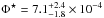 Mpc-3,
L⋆ = 5 ×
1042 erg s-1 and α = −1.6), which probe the faint end of the
luminosity function down to L(Ly
α) ~
1041 erg
s-1. We note that although the Subaru/XMM-Newton
Deep Survey does not reach such faint luminosities, using the corresponding
parameters (Ouchi et al. 2008) does not
significantly change our results. The average luminosity of LAEs is then given by
Mpc-3,
L⋆ = 5 ×
1042 erg s-1 and α = −1.6), which probe the faint end of the
luminosity function down to L(Ly
α) ~
1041 erg
s-1. We note that although the Subaru/XMM-Newton
Deep Survey does not reach such faint luminosities, using the corresponding
parameters (Ouchi et al. 2008) does not
significantly change our results. The average luminosity of LAEs is then given by
 (2)We find that the
average luminosity of ESDLAs matches that of LAEs for Lmin ~ 1041 erg
s-1.
(2)We find that the
average luminosity of ESDLAs matches that of LAEs for Lmin ~ 1041 erg
s-1.
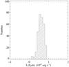 |
Fig. 17 Results from bootstrapping: distribution of the measured mean Ly α luminosities using 300 random subsamples with half the size of the original sample. |
In order to further test whether the Ly α luminosities5 of ESDLA hosts follows that of LAEs with L > 1041 erg s-1, we estimate L in each individual ESDLA by integrating the luminosity within Δv = ±300 km s-1 from the systemic redshift. The corresponding luminosity distribution is shown as grey histogram in Fig. 18. As expected due to the large uncertainties in individual measurements, the distribution is wide and nearly Gaussian. However, we do find that the mean is offset from zero and observe a tail at positive values. We note that the distribution does not change significantly (but gets noisier) when we subtract the mean luminosity per unit wavelength on both sides of the Ly α region (Δv = ± [700−1000] km s-1 from the systemic redshift) before integrating over the central region (blue hashed histogram). This again shows that a possible systematic positive zero-flux offset has no significant effect on the results. We perform a Monte-Carlo analysis by generating a population of 100 000 LAEs with L > 1041 erg s-1 that follows the Cassata et al. (2011) luminosity function (solid red curve in Fig. 18). We randomly added Gaussian noise with σ = 0.9 × 1042 erg s-1 to mimic typical measurement uncertainties6. The resulting distribution (red unfilled histogram) follows the observed one very well. LAEs with L > 5 × 1042 erg s-1 are expected to occur about a hundred times less frequently than those with L > 1041 erg s-1, consistently with the fact that only one ESDLA in our sample has a Ly α line with L > 5 × 1042 erg s-1 (see Fig. 15). The Ly α luminosity measured from follow-up observations on Magellan/MagE and VLT/X-shooter of this system is L ~ 6 × 1042 erg s-1 (Noterdaeme et al. 2012a).
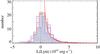 |
Fig. 18 Distribution of Ly α luminosities estimated in individual ESDLAs (grey filled histogram). The blue hashed histogram represents the distribution after subtracting the mean luminosity observed on both sides of the Ly α region. The solid red curve represents the LAE luminosity function from Cassata et al. (2011) (arbitrary scaling), and the red unfilled histogram gives the expected distribution of L ≥ 1041 erg s-1 LAEs when Gaussian noise is added to mimic measurement uncertainties. |
6.4. Ly α profile
Because of resonant scattering, the Ly α line has a complex structure in absorption and emission. Often the two are kinetically displaced. Where possible, Shapley et al. (2003) measured a mean difference of about 650 km s-1 between the absorption from metal lines and the peak of the Ly α emission in LBGs, which suggests that large-scale outflows are common in these objects. In the case of LAEs, spectroscopic observations indicate a velocity difference of about 150 km s-1 between Ly α in emission and non-resonant lines (McLinden et al. 2011; Finkelstein et al. 2011; Hashimoto et al. 2013), i.e. much less than the 400 km s-1 derived for LBGs (Steidel et al. 2010; Shapley et al. 2003).
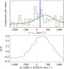 |
Fig. 19 Top: velocity offset of the Ly α profile compared to the systemic redshift. The black histogram shows the stacked ESDLA spectrum, the green line represents the LBG composite (Shapley et al. 2003, scaled down for illustration purposes) and the vertical blue line marks the typical velocity shift observed in LAEs (McLinden et al. 2011; Finkelstein et al. 2011; Hashimoto et al. 2013). Bottom: cross-correlation function obtained by correlating the Lyman-break galaxy and the ESDLA (3σ-clipped mean luminosity) composites at different velocities. The Ly α emission in the LBG composite is redshifted compared to that of ESDLAs by about 250 km s-1. The ESDLA Ly α emission redshift is much closer to the systemic redshift from the low-ionisation metal lines. . |
In the present case, our spectra do not cover NIR emission lines. However, because the line of sight passes through the galaxy, the systemic redshift can be well estimated from the absorption lines, unlike LBGs that have ISM absorption lines arising only from the gas located between the central star-forming region and the observer. For each system in our sample, we carefully measured the redshift from low-ionisation metal lines, cross-correlating the spectrum with a metal template to derive a first guess. We estimate the accuracy to be better than the pixel size, i.e., a few 10 km s-1. This shows that the Ly α profile is slightly shifted toward the red relative to the systemic redshift (see top panel of Fig. 19). This shift is comparable to what is seen in LAEs and significantly (~250 km s-1) less than what is typical of LBGs (bottom panel of Fig. 19). There is also a hint of a double or multiple peaked profile (as described in Kulas et al. 2012), that is seen in the three different composite spectra, but the S/N achieved is still too low to be conclusive.
It is initially somewhat surprising that such high H i column densities do not introduce larger velocity offsets, as the Ly α photons need to scatter away from the line centre to escape (e.g. Neufeld 1990). However, the column density measured along the line of sight is the total column density, and an inhomogeneous ISM could decrease the number of scattering required by Ly α photons to escape the medium (e.g. Finkelstein et al. 2011). Indeed, Ly α transfer is a complex process that depends on ISM clumpiness, kinematics, dust attenuation and geometry (e.g. Haiman & Spaans 1999). In the case of J1135−0010, an escape fraction as high as 0.20 is observed, with a double-peaked profile and little velocity offset, in spite of a very high associated H i column density. In this particular case, the model that successfully reproduces all observable includes anisotropic galactic winds and distributes the total column density across numerous low-N(H i) clouds. However, broadly speaking, the small shift of the Ly α profile in our stacked spectrum indicates kinematic fields with velocities relatively low compared to LBGs and probably lower mass systems on average (Zheng et al. 2010).
6.5. Incidences of ESDLAs and LAEs
In the previous subsections, we found that the distribution, mean value, and shape of the Ly α emission agree with that of emission-selected LAEs with L > 1041 erg s-1. Here, we compare the incidence of this population of LAEs with that of ESDLAs along the QSO lines of sight.
Integrating fHI(N,χ) over
N(H i) ≥ 0.5 ×
1022 cm-2, we derive the number of ESDLA per unit absorption
distance dNESDLA/dχ
≈ 7 × 10⁻⁴. Using
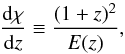 (3)where
 ,
and the co-moving distance per unit redshift,
,
and the co-moving distance per unit redshift,
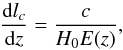 (4)we get
 (5)On the other hand,
the co-moving incidence of LAEs that give rise to ESDLAs can be written as
(5)On the other hand,
the co-moving incidence of LAEs that give rise to ESDLAs can be written as  (6)where
 and rgas is the mean
physical projected extent of the gas with N(H i) ≥ 5 ×
1021 cm-2. By equating Eqs. (5) and (6) at
⟨z⟩ = 2.5,
we derive rgas ≈
2.5 kpc. In other words, the expected number density of LAEs within an
impact parameter of 2.5 kpc from the quasar lines of sight accounts for the incidence of
ESDLAs, in very good agreement with our hypothesis. We also emphasise that this value is
significantly smaller than the SDSS fibre radius (1″ corresponding to ~8 kpc at z ~ 2.5), indicating that
fibre losses are likely negligible and not a problem for our study7. Finally, we note that if our measured Ly α luminosity is
overestimated due to zero-flux offset, then the luminosity function should be integrated
down to lower Lmin, and hence we would derive an even
smaller high-column density gas radius (or equivalently impact parameter).
and rgas is the mean
physical projected extent of the gas with N(H i) ≥ 5 ×
1021 cm-2. By equating Eqs. (5) and (6) at
⟨z⟩ = 2.5,
we derive rgas ≈
2.5 kpc. In other words, the expected number density of LAEs within an
impact parameter of 2.5 kpc from the quasar lines of sight accounts for the incidence of
ESDLAs, in very good agreement with our hypothesis. We also emphasise that this value is
significantly smaller than the SDSS fibre radius (1″ corresponding to ~8 kpc at z ~ 2.5), indicating that
fibre losses are likely negligible and not a problem for our study7. Finally, we note that if our measured Ly α luminosity is
overestimated due to zero-flux offset, then the luminosity function should be integrated
down to lower Lmin, and hence we would derive an even
smaller high-column density gas radius (or equivalently impact parameter).
6.6. Star-formation rate
Assuming case B recombination, the Ly
α to H α ratio is theoretically 8.7. Since this does not
take into account dust and escape fraction corrections, the Ly α luminosity provides a
lower-limit on the star-formation rate. Using the H α−SFR calibration from Kennicutt (1998a),
 (7)we get SFR
(M⊙
yr-1) = 0.9
L(Ly
α)/fesc, where
L(Ly
α) is the observed Ly α luminosity in units of
1042 erg
s-1. This gives
(7)we get SFR
(M⊙
yr-1) = 0.9
L(Ly
α)/fesc, where
L(Ly
α) is the observed Ly α luminosity in units of
1042 erg
s-1. This gives
 (8)in good agreement
with what is expected for most DLAs from cosmological hydrodynamic simulations in a
standard cold dark matter model (Cen 2012). At low
redshift, Kennicutt (1998b) derives the best fit
relation:
(8)in good agreement
with what is expected for most DLAs from cosmological hydrodynamic simulations in a
standard cold dark matter model (Cen 2012). At low
redshift, Kennicutt (1998b) derives the best fit
relation: 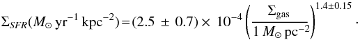 (9)Applying this to
the mean gas surface density, N(H i) ≈ 1021.8cm-2 in our sample, we expect
ΣSFR ≈ 0.08
M⊙ yr-1 kpc-2. From
the integrated SFR derived above, we can write:
(9)Applying this to
the mean gas surface density, N(H i) ≈ 1021.8cm-2 in our sample, we expect
ΣSFR ≈ 0.08
M⊙ yr-1 kpc-2. From
the integrated SFR derived above, we can write:
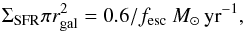 (10)where rgal is the
radius of the system. In the limiting case, fesc = 1, the expected surface
star-formation rate will match the observed integrated SFR if it remains constant over an
effective galaxy radius of rgal ~ 1.5 kpc. In the real situation,
the escape fraction will be smaller than unity. For the global population of
high-z
galaxies, Hayes et al. (2010) estimate
fesc =
0.05, which would imply rgal ~ 6 kpc, i.e., a significant
fraction of the galaxy light could easily fall outside the BOSS fibre. However, the
typical escape fraction for high-z LAEs is significantly higher, about
fesc ≈
0.30 (Blanc et al. 2011; Nakajima et al. 2012)8, implying rgal ~ 2.5 kpc. While the
~35% uncertainty on the
Ly α
luminosity propagates to 17% on rgas, we caution that this remains a
simple model ignoring projection effects and where the most important unknown remains the
escape fraction. With these limitations in mind, we can say that our overall picture is
satisfactorally consistent. Indeed, the emission radius (rgal) matches
the high column density radius estimated above (rgas), further indicating that ESDLAs do
arise from lines of sight passing through the ISM which feeds star-formation. This result
also matches expectations from hydrodynamical simulations (e.g. Altay et al. 2013).
(10)where rgal is the
radius of the system. In the limiting case, fesc = 1, the expected surface
star-formation rate will match the observed integrated SFR if it remains constant over an
effective galaxy radius of rgal ~ 1.5 kpc. In the real situation,
the escape fraction will be smaller than unity. For the global population of
high-z
galaxies, Hayes et al. (2010) estimate
fesc =
0.05, which would imply rgal ~ 6 kpc, i.e., a significant
fraction of the galaxy light could easily fall outside the BOSS fibre. However, the
typical escape fraction for high-z LAEs is significantly higher, about
fesc ≈
0.30 (Blanc et al. 2011; Nakajima et al. 2012)8, implying rgal ~ 2.5 kpc. While the
~35% uncertainty on the
Ly α
luminosity propagates to 17% on rgas, we caution that this remains a
simple model ignoring projection effects and where the most important unknown remains the
escape fraction. With these limitations in mind, we can say that our overall picture is
satisfactorally consistent. Indeed, the emission radius (rgal) matches
the high column density radius estimated above (rgas), further indicating that ESDLAs do
arise from lines of sight passing through the ISM which feeds star-formation. This result
also matches expectations from hydrodynamical simulations (e.g. Altay et al. 2013).
6.7. Dependence on dust
In this section, we wish to study the effect of dust on the Ly α emission as attenuation by dust is known to have a significant impact on the Ly α escape fraction. High-redshift LAEs, like ESDLAs have a generally low dust content, with E(B − V) ~ 0−0.07 at z ~ 3 (Nilsson et al. 2007; Ono et al. 2010), although it evolves significantly from z ~ 3 to z ~ 2 (Guaita et al. 2011; Nakajima et al. 2012). However, due to resonant scattering, the optical path of Ly α photons can be very different and longer than that of photons from the UV continuum or non-resonant lines like Hα or Hβ. Consequently, even a small amount of dust can affect the Ly α escape fraction.
Blanc et al. (2011) report a correlation between the Ly α equivalent width and reddening in high-z LAEs. Similarly, Atek et al. (2014) observe a clear dependence of the Ly α escape fraction on the dust extinction in nearby galaxies.
Moreover, we note that galaxies hosting high-metallicity, dust-rich DLAs generally have no detectable Ly α emission, despite their high star-formation rates (Fynbo et al. 2013). As an additional difficulty, here, we have access only to the extinction along the QSO line of sight. Because the impact parameter is small, we can, however, expect this extinction to be similar to that in the star-forming region as evidenced in e.g. Gupta et al. (2013).
We thus divide our sample into two subsamples with E(B − V) below and above the median E(B − V) value and perform two independent stacks with the accompanying bootstrap analysis (using random samples half the size of each subsample), see Fig. 20. The Ly α luminosity is four times higher in the less dusty subsample, with ⟨L(Ly α)⟩ ~ 1042 erg s-1, compared to ⟨L(Ly α)⟩ ~ 0.25 × 1042 erg s-1 in the dustier subsample. This is consistent with larger escape fractions for less dusty systems.
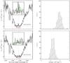 |
Fig. 20 Effect of dust on the Ly α emission. The 3 σ-clipped mean luminosity are represented on the left panels and the corresponding bootstrap analysis on the right panels. The top (respectively bottom) panels correspond to the ESDLA subsample with E(B − V) < 0.025 (respectively E(B − V) ≥ 0.025). |
7. Conclusion
The historical N(H i)-threshold for DLAs, log N(H i) ≥ 20.3, was originally chosen mostly for observational reasons (Wolfe et al. 1986) and was found similar to H i column densities measured in the disks of local spiral galaxies. However, it is becoming more and more clear that a significant fraction of DLAs at high redshift probe gas on the outskirts of a galaxy. Recent 21-cm observations of nearby galaxies have shown that higher H i column densities are mostly found at small impact parameters (~80% probability of being located at less than 5 kpc for log N(H i) ≥ 21.7, Zwaan et al. 2005). At high redshift, simulations also indicate that only the highest column density absorptions probe ISM gas that feeds star formation (e.g. Altay et al. 2013; Rahmati et al. 2013; Rahmati & Schaye 2014). Here, we have studied an elusive population of extremely strong DLAs detected in BOSS. The small incidence of these systems reflects their small cross-section. Confirming our previous result in (see Noterdaeme et al. 2012b), the high column density end of the N(H i)-distribution function has a moderate power-law slope, similar to that of the local Universe. We find that the metallicities and dust-depletion of ESDLAs are similar to those of the overall DLA population and thus indicate that they are related to a similar population of galaxies. Their higher column densities are mainly the consequence of small impact parameters. Indeed, we found that the absorption characteristics are very similar to what is seen in DLAs associated with GRB afterglows, which are known to be intimately related to star-formation regions.
Using stacking techniques, we detect Ly
α emission in the core of ESDLAs with a mean
luminosity  which corresponds to that of LLy α ≥
1041 erg
s-1 Lyman-α emitting galaxies. We also show that the
distribution of luminosities measured in individual spectra, although noisy, is also
consistent with that of the above LAE population.
which corresponds to that of LLy α ≥
1041 erg
s-1 Lyman-α emitting galaxies. We also show that the
distribution of luminosities measured in individual spectra, although noisy, is also
consistent with that of the above LAE population.
The incidences of ESDLAs and LAEs indicate impact parameters b < 2.5 kpc. The properties of the Lyα emission in both populations are very similar. All of this strongly suggests that the ESDLA host galaxies are actually LAEs that emit most of their light well within the area covered by the BOSS fibre (8 kpc radius) and obey the Schmidt-Kennicutt law. We caution however that the measured Ly α luminosity may be overestimated by ~35% due to sky light residuals and/or FUV emission from the QSO host and that we have neglected flux-calibration uncertainties. However, this has little consequence on our overall picture. Indeed, a lower Ly α luminosity would imply a fainter but more numerous LAE population (hence a smaller extent of gas to match the incidence of ESDLAs) and at the same time a smaller galactic size according to the Schmidt-Kennicutt law.
Hashimoto et al. (2013) recently suggested that LAEs should have small neutral hydrogen column densities. However, this suggestion arises from considerations based on homogeneous expanding shell models (Verhamme et al. 2006), while the true configuration is probably much more complicated (e.g. Kulas et al. 2012). Indeed, recent works have highlighted the importance of ISM clumpiness and geometry in allowing Ly α photons to escape from star-forming regions (e.g. Laursen et al. 2013), even at high integrated H i column densities (e.g. Noterdaeme et al. 2012a). Finally we note that the viewing angle seems to play an important role in anisotropic configurations (Zheng & Wallace 2013).
Interestingly, using very deep (92 h of VLT/FORS2) long-slit spectroscopy, Rauch et al. (2008) revealed a population of faint LAEs with L(Ly α) ~ 1041 erg s-1 that have a total cross-section consistent with that of DLAs (see also Barnes & Haehnelt 2009). Targeting high-metallicity DLAs has successfully produced a number of host galaxy detections with higher SFR, but the host galaxies are frequently at large impact parameters and either have no Ly α emission or a suppressed blue peak (see Fynbo et al. 2010, 2011, 2013; Krogager et al. 2012, 2013). This indicates that high metallicity DLAs could be associated with massive and luminous galaxies, but their cross-section selection increases the probability that the DLAs will probe the galaxy outskirts. This is in line with other studies suggesting that the large cross-section of gas around massive galaxies is responsible for higher metallicities in sub-DLAs on average (Khare et al. 2007; Kulkarni et al. 2010). ESDLAs, however, are selected solely on the basis of high H i column densities. They should arise in more typical galaxies that have not yet converted their gas reservoirs into stars and thereby produced little metals, as seen from the low metallicities.
Follow-up studies of ESDLAs and their host galaxies will contribute important clues for understanding galaxy formation at high redshift and constrain crucial parameters for numerical simulations such as the amount of stellar feedback and the gas consumption rate. In particular, deep multi-wavelength spectroscopy, covering both Ly α and nebular emission lines (redshifted in the near-infrared) are required to measure accurately the star-formation rate and hence the Ly α escape fraction as well as bringing constraints on the Ly α transfer.
Online material
Intervening ESDLA sample.
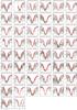 |
Fig. 21 Normalised flux (black, 3 pixel boxcar smoothed) and error (orange) around the damped Ly α line. The Voigt-profile fit is overplotted in red, with the shaded area corresponding to an uncertainty of 0.2 dex. The QSO name, DLA resdshift and H i column density are indicated above each panel. |
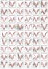 |
Fig. 21 continued. |
We note that the data quality is not good enough to observationally test the theoretical assymetry of the strong damped Ly α and Ly β profiles recently calculated by Lee (2013).
The continuum-to-noise ratio is averaged over the Ly α-forest, 5000 km s-1 redwards (resp. bluewards) of the Ly β (resp. Ly α) emission line. See Noterdaeme et al. (2009, 2012b) for more details.
We caution however that the derivation of E(B − V) here and in Vladilo et al. (2008) are quite different, the former being based on SED fitting with a template and the latter based on photometric colour excess.
Noterdaeme et al. (2012a) analysed this system and derived SFR ~ 25 M⊙ yr-1 from the detection of H α emission.
To simplify the writing, here and in the following, “L” implicitly stands for Ly α luminosity, i.e. “L(Ly α)”.
This corresponds to the 0.09 × 1042 erg s-1 statistical uncertainty on the mean, scaled up by the square root of the number of systems used for the stack.
See discussions in López & Chen (2012) about the dangers of associating a population of extended absorbers with emitting galaxies in aperture-limited surveys.
The follow-up observations of the ESDLA towards J1135−0010 indicate fesc ~ 0.2.
Acknowledgments
We thank the referee for careful reading as well as constructive comments and suggestions and Susanna Vergani for helpful discussions. The SDSS-III French participation group was supported by the Agence Nationale de la Recherche under grants ANR-08-BLAN-0222 and ANR-12-BS05-0015. Funding for SDSS-III has been provided by the Alfred P. Sloan Foundation, the Participating Institutions, the National Science Foundation, and the US Department of Energy Office of Science. The SDSS-III website is http://www.sdss3.org/. SDSS-III is managed by the Astrophysical Research Consortium for the Participating Institutions of the SDSS-III Collaboration including the University of Arizona, the Brazilian Participation Group, Brookhaven National Laboratory, University of Cambridge, Carnegie Mellon University, University of Florida, the French Participation Group, the German Participation Group, Harvard University, the Instituto de Astrofísica de Canarias, the Michigan State/Notre Dame/JINA Participation Group, Johns Hopkins University, Lawrence Berkeley National Laboratory, Max Planck Institute for Astrophysics, Max Planck Institute for Extraterrestrial Physics, New Mexico State University, New York University, Ohio State University, Pennsylvania State University, University of Portsmouth, Princeton University, the Spanish Participation Group, University of Tokyo, University of Utah, Vanderbilt University, University of Virginia, University of Washington, and Yale University.
References
- Adams, J. J., Blanc, G. A., Hill, G. J., et al. 2011, ApJS, 192, 5 [NASA ADS] [CrossRef] [Google Scholar]
- Ahn, C. P., Alexandroff, R., Allen de Prieto, C., et al. 2012, ApJS, 203, 21 [NASA ADS] [CrossRef] [Google Scholar]
- Ahn, C. P., Alexandroff, R., Allen de Prieto, C., et al. 2014, ApJS, 211, 17 [NASA ADS] [CrossRef] [Google Scholar]
- Altay, G., & Theuns, T. 2013, MNRAS, 434, 748 [NASA ADS] [CrossRef] [Google Scholar]
- Altay, G., Theuns, T., Schaye, J., Booth, C. M., & Dal la Vecchia, C. 2013, MNRAS, 436, 2689 [NASA ADS] [CrossRef] [Google Scholar]
- Atek, H., Kunth, D., Schaerer, D., et al. 2014, A&A, 561, A89 [NASA ADS] [CrossRef] [EDP Sciences] [Google Scholar]
- Balashev, S. A., Klimenko, V. V., Ivanchik, A. V., et al. 2014, MNRAS, 440, 225 [NASA ADS] [CrossRef] [Google Scholar]
- Barnes, L. A., & Haehnelt, M. G. 2009, MNRAS, 397, 511 [NASA ADS] [CrossRef] [Google Scholar]
- Blanc, G. A., Adams, J. J., Gebhardt, K., et al. 2011, ApJ, 736, 31 [NASA ADS] [CrossRef] [Google Scholar]
- Bloom, J. S., Kulkarni, S. R., Djorgovski, S. G., et al. 1999, Nature, 401, 453 [NASA ADS] [CrossRef] [Google Scholar]
- Bolton, A. S., Schlegel, D. J., Aubourg, É., et al. 2012, AJ, 144, 144 [NASA ADS] [CrossRef] [Google Scholar]
- Bouché, N., Murphy, M. T., Péroux, C., et al. 2012, MNRAS, 419, 2 [NASA ADS] [CrossRef] [Google Scholar]
- Bouché, N., Murphy, M. T., Kacprzak, G. G., et al. 2013, Science, 341, 50 [NASA ADS] [CrossRef] [Google Scholar]
- Braun, R. 2012, ApJ, 749, 87 [NASA ADS] [CrossRef] [Google Scholar]
- Cai, Z., Fan, X., Noterdaeme, P., et al. 2014, ApJ, submitted [Google Scholar]
- Cassata, P., Le Fèvre, O., Garilli, B., et al. 2011, A&A, 525, A143 [NASA ADS] [CrossRef] [EDP Sciences] [Google Scholar]
- Cen, R. 2012, ApJ, 748, 121 [NASA ADS] [CrossRef] [Google Scholar]
- Chelouche, D., & Bowen, D. V. 2010, ApJ, 722, 1821 [NASA ADS] [CrossRef] [Google Scholar]
- Ciardullo, R., Gronwall, C., Wolf, C., et al. 2012, ApJ, 744, 110 [NASA ADS] [CrossRef] [Google Scholar]
- Cowie, L. L., & Hu, E. M. 1998, AJ, 115, 1319 [NASA ADS] [CrossRef] [Google Scholar]
- Daddi, E., Dannerbauer, H., Stern, D., et al. 2009, ApJ, 694, 1517 [Google Scholar]
- Dawson, K. S., Schlegel, D. J., Ahn, C. P., et al. 2013, AJ, 145, 10 [Google Scholar]
- De Cia, A., Ledoux, C., Savaglio, S., Schady, P., & Vreeswijk, P. M. 2013, A&A, 560, A88 [NASA ADS] [CrossRef] [EDP Sciences] [Google Scholar]
- de Ugarte Postigo, A., Fynbo, J. P. U., Thöne, C. C., et al. 2012, A&A, 548, A11 [NASA ADS] [CrossRef] [EDP Sciences] [Google Scholar]
- Eisenstein, D. J., Weinberg, D. H., Agol, E., et al. 2011, AJ, 142, 72 [Google Scholar]
- Ellison, S. L. 2006, MNRAS, 368, 335 [NASA ADS] [CrossRef] [Google Scholar]
- Ellison, S. L., Prochaska, J. X., Hennawi, J., et al. 2010, MNRAS, 406, 1435 [NASA ADS] [Google Scholar]
- Finkelstein, S. L., Cohen, S. H., Windhorst, R. A., et al. 2011, ApJ, 735, 5 [NASA ADS] [CrossRef] [Google Scholar]
- Finley, H., Petitjean, P., Pâris, I., et al. 2013, A&A, 558, A111 [Google Scholar]
- Fox, A. J., Petitjean, P., Ledoux, C., & Srianand, R. 2007, A&A, 465, 171 [NASA ADS] [CrossRef] [EDP Sciences] [Google Scholar]
- Fumagalli, M., O’Meara, J. M., & Prochaska, J. X. 2011, Science, 334, 1245 [NASA ADS] [CrossRef] [Google Scholar]
- Fynbo, J. P. U., Jakobsson, P., Prochaska, J. X., et al. 2009, ApJS, 185, 526 [NASA ADS] [CrossRef] [Google Scholar]
- Fynbo, J. P. U., Laursen, P., Ledoux, C., et al. 2010, MNRAS, 408, 2128 [NASA ADS] [CrossRef] [Google Scholar]
- Fynbo, J. P. U., Ledoux, C., Noterdaeme, P., et al. 2011, MNRAS, 413, 2481 [NASA ADS] [CrossRef] [Google Scholar]
- Fynbo, J. P. U., Geier, S. J., Christensen, L., et al. 2013, MNRAS, 436, 361 [NASA ADS] [CrossRef] [Google Scholar]
- Gawiser, E., Francke, H., Lai, K., et al. 2007, ApJ, 671, 278 [NASA ADS] [CrossRef] [Google Scholar]
- Gillmon, K., Shull, J. M., Tumlinson, J., & Danforth, C. 2006, ApJ, 636, 891 [NASA ADS] [CrossRef] [Google Scholar]
- Guaita, L., Acquaviva, V., Padilla, N., et al. 2011, ApJ, 733, 114 [NASA ADS] [CrossRef] [Google Scholar]
- Guimarães, R., Noterdaeme, P., Petitjean, P., et al. 2012, AJ, 143, 147 [NASA ADS] [CrossRef] [Google Scholar]
- Gunn, J. E., Siegmund, W. A., Mannery, E. J., et al. 2006, AJ, 131, 2332 [NASA ADS] [CrossRef] [Google Scholar]
- Gupta, N., Srianand, R., Noterdaeme, P., Petitjean, P., & Muzahid, S. 2013, A&A, 558, A84 [NASA ADS] [CrossRef] [EDP Sciences] [Google Scholar]
- Haehnelt, M. G., Steinmetz, M., & Rauch, M. 1998, ApJ, 495, 647 [NASA ADS] [CrossRef] [Google Scholar]
- Haiman, Z., & Spaans, M. 1999, ApJ, 518, 138 [NASA ADS] [CrossRef] [Google Scholar]
- Hashimoto, T., Ouchi, M., Shimasaku, K., et al. 2013, ApJ, 765, 70 [NASA ADS] [CrossRef] [Google Scholar]
- Hayes, M., Östlin, G., Schaerer, D., et al. 2010, Nature, 464, 562 [NASA ADS] [CrossRef] [PubMed] [Google Scholar]
- Hu, E. M., Cowie, L. L., & McMahon, R. G. 1998, ApJ, 502, L99 [NASA ADS] [CrossRef] [Google Scholar]
- Jorgenson, R. A., Murphy, M. T., & Thompson, R. 2013, MNRAS, 435, 482 [NASA ADS] [CrossRef] [Google Scholar]
- Kashikawa, N., Misawa, T., Minowa, Y., et al. 2014, ApJ, 780, 116 [NASA ADS] [CrossRef] [Google Scholar]
- Kauffmann, G. 1996, MNRAS, 281, 487 [NASA ADS] [CrossRef] [Google Scholar]
- Kennicutt, Jr., R. C. 1998a, ARA&A, 36, 189 [Google Scholar]
- Kennicutt, Jr., R. C. 1998b, ApJ, 498, 541 [NASA ADS] [CrossRef] [Google Scholar]
- Khare, P., Kulkarni, V. P., Péroux, C., et al. 2007, A&A, 464, 487 [NASA ADS] [CrossRef] [EDP Sciences] [Google Scholar]
- Khare, P., van den Berk, D., York, D. G., Lundgren, B., & Kulkarni, V. P. 2012, MNRAS, 419, 1028 [NASA ADS] [CrossRef] [Google Scholar]
- Koen, C., & Kondlo, L. 2009, MNRAS, 397, 495 [NASA ADS] [CrossRef] [Google Scholar]
- Kornei, K. A., Shapley, A. E., Erb, D. K., et al. 2010, ApJ, 711, 693 [NASA ADS] [CrossRef] [Google Scholar]
- Krogager, J.-K., Fynbo, J. P. U., Møller, P., et al. 2012, MNRAS, 424, L1 [NASA ADS] [CrossRef] [Google Scholar]
- Krogager, J.-K., Fynbo, J. P. U., Ledoux, C., et al. 2013, MNRAS, 433, 3091 [NASA ADS] [CrossRef] [Google Scholar]
- Kulas, K. R., Shapley, A. E., Kollmeier, J. A., et al. 2012, ApJ, 745, 33 [NASA ADS] [CrossRef] [Google Scholar]
- Kulkarni, V. P., Khare, P., Som, D., et al. 2010, New A, 15, 735 [Google Scholar]
- Kulkarni, V. P., Meiring, J., Som, D., et al. 2012, ApJ, 749, 176 [NASA ADS] [CrossRef] [Google Scholar]
- Lai, K., Huang, J.-S., Fazio, G., et al. 2008, ApJ, 674, 70 [NASA ADS] [CrossRef] [Google Scholar]
- Laursen, P., Duval, F., & Östlin, G. 2013, ApJ, 766, 124 [NASA ADS] [CrossRef] [Google Scholar]
- Ledoux, C., Petitjean, P., Bergeron, J., Wampler, E. J., & Srianand, R. 1998, A&A, 337, 51 [NASA ADS] [Google Scholar]
- Ledoux, C., Petitjean, P., & Srianand, R. 2003, MNRAS, 346, 209 [NASA ADS] [CrossRef] [Google Scholar]
- Ledoux, C., Petitjean, P., Fynbo, J. P. U., Møller, P., & Srianand, R. 2006, A&A, 457, 71 [NASA ADS] [CrossRef] [EDP Sciences] [MathSciNet] [Google Scholar]
- Lee, H.-W. 2013, ApJ, 772, 123 [NASA ADS] [CrossRef] [Google Scholar]
- López, G., & Chen, H.-W. 2012, MNRAS, 419, 3553 [NASA ADS] [CrossRef] [Google Scholar]
- Lowenthal, J. D., Hogan, C. J., Green, R. F., et al. 1995, ApJ, 451, 484 [NASA ADS] [CrossRef] [Google Scholar]
- McLinden, E. M., Finkelstein, S. L., Rhoads, J. E., et al. 2011, ApJ, 730, 136 [NASA ADS] [CrossRef] [Google Scholar]
- Møller, P., Fynbo, J. P. U., & Fall, S. M. 2004, A&A, 422, L33 [NASA ADS] [CrossRef] [EDP Sciences] [Google Scholar]
- Møller, P., Fynbo, J. P. U., Ledoux, C., & Nilsson, K. K. 2013, MNRAS, 430, 2680 [NASA ADS] [CrossRef] [Google Scholar]
- Nakajima, K., Ouchi, M., Shimasaku, K., et al. 2012, ApJ, 745, 12 [NASA ADS] [CrossRef] [Google Scholar]
- Nestor, D. B., Rao, S. M., Turnshek, D. A., & Van den Berk, D. 2003, ApJ, 595, L5 [NASA ADS] [CrossRef] [Google Scholar]
- Neufeld, D. A. 1990, ApJ, 350, 216 [NASA ADS] [CrossRef] [Google Scholar]
- Nilsson, K. K., Møller, P., Möller, O., et al. 2007, A&A, 471, 71 [NASA ADS] [CrossRef] [EDP Sciences] [Google Scholar]
- Noterdaeme, P., Ledoux, C., Petitjean, P., et al. 2007a, A&A, 474, 393 [Google Scholar]
- Noterdaeme, P., Petitjean, P., Srianand, R., Ledoux, C., & Le Petit, F. 2007b, A&A, 469, 425 [NASA ADS] [CrossRef] [EDP Sciences] [Google Scholar]
- Noterdaeme, P., Ledoux, C., Petitjean, P., & Srianand, R. 2008, A&A, 481, 327 [NASA ADS] [CrossRef] [EDP Sciences] [Google Scholar]
- Noterdaeme, P., Petitjean, P., Ledoux, C., & Srianand, R. 2009, A&A, 505, 1087 [NASA ADS] [CrossRef] [EDP Sciences] [Google Scholar]
- Noterdaeme, P., Petitjean, P., Ledoux, C., et al. 2010, A&A, 523, A80 [NASA ADS] [CrossRef] [EDP Sciences] [Google Scholar]
- Noterdaeme, P., Laursen, P., Petitjean, P., et al. 2012a, A&A, 540, A63 [NASA ADS] [CrossRef] [EDP Sciences] [Google Scholar]
- Noterdaeme, P., Petitjean, P., Carithers, W. C., et al. 2012b, A&A, 547, L1 [NASA ADS] [CrossRef] [EDP Sciences] [Google Scholar]
- Omont, A., Petitjean, P., Guilloteau, S., et al. 1996, Nature, 382, 428 [NASA ADS] [CrossRef] [PubMed] [Google Scholar]
- Ono, Y., Ouchi, M., Shimasaku, K., et al. 2010, ApJ, 724, 1524 [NASA ADS] [CrossRef] [Google Scholar]
- Ouchi, M., Shimasaku, K., Akiyama, M., et al. 2008, ApJS, 176, 301 [NASA ADS] [CrossRef] [Google Scholar]
- Pâris, I., Petitjean, P., Aubourg, É., et al. 2012, A&A, 548, A66 [NASA ADS] [CrossRef] [EDP Sciences] [Google Scholar]
- Pâris, I., Petitjean, P., Aubourg, É., et al. 2014, A&A, 563, A54 [NASA ADS] [CrossRef] [EDP Sciences] [Google Scholar]
- Péroux, C., McMahon, R. G., Storrie-Lombardi, L. J., & Irwin, M. J. 2003, MNRAS, 346, 1103 [NASA ADS] [CrossRef] [Google Scholar]
- Péroux, C., Bouché, N., Kulkarni, V. P., York, D. G., & Vladilo, G. 2011, MNRAS, 410, 2237 [NASA ADS] [CrossRef] [Google Scholar]
- Petitjean, P., Webb, J. K., Rauch, M., Carswell, R. F., & Lanzetta, K. 1993, MNRAS, 262, 499 [NASA ADS] [CrossRef] [Google Scholar]
- Petitjean, P., Pécontal, E., Valls-Gabaud, D., & Chariot, S. 1996, Nature, 380, 411 [NASA ADS] [CrossRef] [Google Scholar]
- Petitjean, P., Ledoux, C., & Srianand, R. 2008, A&A, 480, 349 [NASA ADS] [CrossRef] [EDP Sciences] [Google Scholar]
- Pieri, M. M., Frank, S., Weinberg, D. H., Mathur, S., & York, D. G. 2010, ApJ, 724, L69 [NASA ADS] [CrossRef] [Google Scholar]
- Pontzen, A., Governato, F., Pettini, M., et al. 2008, MNRAS, 390, 1349 [NASA ADS] [Google Scholar]
- Prochaska, J. X., & Wolfe, A. M. 1997, ApJ, 487, 73 [CrossRef] [Google Scholar]
- Prochaska, J. X., & Wolfe, A. M. 1998, ApJ, 507, 113 [NASA ADS] [CrossRef] [Google Scholar]
- Prochaska, J. X., Gawiser, E., Wolfe, A. M., Cooke, J., & Gelino, D. 2003, ApJS, 147, 227 [NASA ADS] [CrossRef] [Google Scholar]
- Prochaska, J. X., Herbert-Fort, S., & Wolfe, A. M. 2005, ApJ, 635, 123 [NASA ADS] [CrossRef] [Google Scholar]
- Prochaska, J. X., Wolfe, A. M., Howk, J. C., et al. 2007, ApJS, 171, 29 [NASA ADS] [CrossRef] [Google Scholar]
- Prochaska, J. X., Chen, H.-W., Wolfe, A. M., Dessauges-Zavadsky, M., & Bloom, J. S. 2008, ApJ, 672, 59 [NASA ADS] [CrossRef] [Google Scholar]
- Prochaska, J. X., Sheffer, Y., Perley, D. A., et al. 2009, ApJ, 691, L27 [NASA ADS] [CrossRef] [Google Scholar]
- Prochaska, J. X., Madau, P., O’Meara, J. M., & Fumagalli, M. 2014, MNRAS, 438, 476 [NASA ADS] [CrossRef] [Google Scholar]
- Rafelski, M., Wolfe, A. M., Prochaska, J. X., Neeleman, M., & Mendez, A. J. 2012, ApJ, 755, 89 [NASA ADS] [CrossRef] [Google Scholar]
- Rahmani, H., Srianand, R., Noterdaeme, P., & Petitjean, P. 2010, MNRAS, 409, L59 [NASA ADS] [Google Scholar]
- Rahmani, H., Wendt, M., Srianand, R., et al. 2013, MNRAS, 435, 861 [NASA ADS] [CrossRef] [Google Scholar]
- Rahmati, A., & Schaye, J. 2014, MNRAS, 438, 529 [NASA ADS] [CrossRef] [Google Scholar]
- Rahmati, A., Schaye, J., Pawlik, A. H., & Raičevic, M., 2013, MNRAS, 431, 2261 [NASA ADS] [CrossRef] [Google Scholar]
- Rauch, M., & Haehnelt, M. G. 2011, MNRAS, 412, L55 [NASA ADS] [CrossRef] [Google Scholar]
- Rauch, M., Haehnelt, M., Bunker, A., et al. 2008, ApJ, 681, 856 [NASA ADS] [CrossRef] [Google Scholar]
- Rhoads, J. E., Malhotra, S., Dey, A., et al. 2000, ApJ, 545, L85 [NASA ADS] [CrossRef] [Google Scholar]
- Savage, B. D., Bohlin, R. C., Drake, J. F., & Budich, W. 1977, ApJ, 216, 291 [NASA ADS] [CrossRef] [Google Scholar]
- Schaye, J. 2001, ApJ, 562, L95 [NASA ADS] [CrossRef] [Google Scholar]
- Schaye, J. 2004, ApJ, 609, 667 [NASA ADS] [CrossRef] [Google Scholar]
- Schechter, P. 1976, ApJ, 203, 297 [Google Scholar]
- Shapley, A. E. 2011, ARA&A, 49, 525 [NASA ADS] [CrossRef] [Google Scholar]
- Shapley, A. E., Steidel, C. C., Pettini, M., & Adelberger, K. L. 2003, ApJ, 588, 65 [NASA ADS] [CrossRef] [Google Scholar]
- Smee, S. A., Gunn, J. E., Uomoto, A., et al. 2013, AJ, 146, 32 [Google Scholar]
- Srianand, R., Petitjean, P., Ledoux, C., Ferland, G., & Shaw, G. 2005, MNRAS, 362, 549 [Google Scholar]
- Srianand, R., Gupta, N., Petitjean, P., Noterdaeme, P., & Saikia, D. J. 2008, MNRAS, 391, L69 [NASA ADS] [Google Scholar]
- Steidel, C. C., Giavalisco, M., Pettini, M., Dickinson, M., & Adelberger, K. L. 1996, ApJ, 462, L17 [NASA ADS] [CrossRef] [Google Scholar]
- Steidel, C. C., Adelberger, K. L., Shapley, A. E., et al. 2003, ApJ, 592, 728 [NASA ADS] [CrossRef] [Google Scholar]
- Steidel, C. C., Erb, D. K., Shapley, A. E., et al. 2010, ApJ, 717, 289 [NASA ADS] [CrossRef] [Google Scholar]
- Tumlinson, J., Shull, J. M., Rachford, B. L., et al. 2002, ApJ, 566, 857 [NASA ADS] [CrossRef] [Google Scholar]
- Van den Berk, D. E., Richards, G. T., Bauer, A., et al. 2001, AJ, 122, 549 [NASA ADS] [CrossRef] [Google Scholar]
- Verhamme, A., Schaerer, D., & Maselli, A. 2006, A&A, 460, 397 [NASA ADS] [CrossRef] [EDP Sciences] [Google Scholar]
- Vladilo, G., & Péroux, C. 2005, A&A, 444, 461 [NASA ADS] [CrossRef] [EDP Sciences] [Google Scholar]
- Vladilo, G., Prochaska, J. X., & Wolfe, A. M. 2008, A&A, 478, 701 [NASA ADS] [CrossRef] [EDP Sciences] [Google Scholar]
- Vreeswijk, P. M., Ledoux, C., Smette, A., et al. 2007, A&A, 468, 83 [NASA ADS] [CrossRef] [EDP Sciences] [Google Scholar]
- Welty, D. E., Lauroesch, J. T., Blades, J. C., Hobbs, L. M., & York, D. G. 1997, ApJ, 489, 672 [NASA ADS] [CrossRef] [Google Scholar]
- Welty, D. E., Frisch, P. C., Sonneborn, G., & York, D. G. 1999, ApJ, 512, 636 [NASA ADS] [CrossRef] [Google Scholar]
- Wolfe, A. M., Turnshek, D. A., Smith, H. E., & Cohen, R. D. 1986, ApJS, 61, 249 [NASA ADS] [CrossRef] [Google Scholar]
- Wolfe, A. M., Prochaska, J. X., & Gawiser, E. 2003, ApJ, 593, 215 [NASA ADS] [CrossRef] [Google Scholar]
- Wolfe, A. M., Gawiser, E., & Prochaska, J. X. 2005, ARA&A, 43, 861 [NASA ADS] [CrossRef] [MathSciNet] [Google Scholar]
- Yajima, H., Choi, J.-H., & Nagamine, K. 2012, MNRAS, 427, 2889 [NASA ADS] [CrossRef] [Google Scholar]
- York, D. G., Adelman, J., Anderson, Jr., J. E., et al. 2000, AJ, 120, 1579 [Google Scholar]
- York, D. G., Khare, P., Van den Berk, D., et al. 2006, MNRAS, 367, 945 [NASA ADS] [CrossRef] [Google Scholar]
- Zafar, T., Møller, P., Ledoux, C., et al. 2011, A&A, 532, A51 [NASA ADS] [CrossRef] [EDP Sciences] [Google Scholar]
- Zafar, T., Péroux, C., Popping, A., et al. 2013, A&A, 556, A141 [NASA ADS] [CrossRef] [EDP Sciences] [Google Scholar]
- Zheng, Z., & Wallace, J. 2013, AJ, submitted [arXiv:1308.1405] [Google Scholar]
- Zheng, Z., Cen, R., Trac, H., & Miralda-Escudé, J. 2010, ApJ, 716, 574 [NASA ADS] [CrossRef] [Google Scholar]
- Zwaan, M. A., & Prochaska, J. X. 2006, ApJ, 643, 675 [NASA ADS] [CrossRef] [Google Scholar]
- Zwaan, M. A., van der Hulst, J. M., Briggs, F. H., Verheijen, M. A. W., & Ryan-Weber, E. V. 2005, MNRAS, 364, 1467 [NASA ADS] [CrossRef] [Google Scholar]
All Tables
All Figures
|
Fig. 1 DLA N(H i)-distribution function. The high column density end of the distribution studied here is shown in black for the overall DR11 sample and a subset with higher continuum-to-noise ratio (red). Green points show the results from Noterdaeme et al. (2012b) based on DR9. |
| In the text | |
|
Fig. 2 Measured power-law slope as a function of input slope and measurement uncertainty. The different regions (respectively dotted, grey area, dashed) show the 1σ range around the mean value for respectively αi = −3; −3.5 and − 4. |
| In the text | |
|
Fig. 3 Median ESDLA absorption spectrum redwards of the QSO Ly-α emission. The grey line shows the fraction of the total sample contributing to the stacked spectrum at a given wavelength. |
| In the text | |
|
Fig. 4 Distributions of the Si ii λ1526 equivalent width measured in ESDLAs (hashed black histogram) and in a sample representative of the overall population of DLAs (green Jorgenson et al. 2013). The vertical line corresponds to the equivalent width (the 1 σ error is represented by the grey area) measured in the stacked ESDLA spectrum. The inset shows the corresponding cumulative distributions (solid black: ESDLAs, dashed green: Jorgenson et al. 2013). |
| In the text | |
|
Fig. 5 Curve-of-growth for Fe ii (left) and Si ii (right) in the stacked spectrum. |
| In the text | |
|
Fig. 6 Relative abundance pattern derived from measurements in the stacked absorption spectrum. The dotted (respectively dashed) line shows the typical patterns found in the Halo (respectively warm disc) of the Galaxy (see Welty et al. 1999). |
| In the text | |
|
Fig. 7 Velocity width, Δv measured by Ledoux et al. (2006) from VLT/UVES spectra as a function of the effective Doppler parameter derived from the equivalent widths of Fe ii and/or Si ii lines. As expected, the theoretical relation for a single unsaturated component, Δv = 2.33b (dotted line), encompasses the data. The dashed line shows the empirical fitted relation Δv = 2.21 beff + 0.02 beff2. The histogram shows the distribution of beff measured in the sample of Ledoux et al. (2006), with the scale on the right axis. The vertical dashed lines mark the values independently found in ESDLAs from Si ii and Fe ii. |
| In the text | |
|
Fig. 8 Portion of the normalised stacked spectrum around the O vi doublet. |
| In the text | |
|
Fig. 9 H i column density distribution for our intervening QSO-DLAs with N(H i) ≥ 5 × 1022cm-2 (hashed histogram) compared to that of associated GRB-DLAs (red unfilled histogram, Fynbo et al. 2009; de Ugarte Postigo et al. 2012). |
| In the text | |
|
Fig. 10 Rest-frame equivalent widths of metal lines as a function of log N(H i). Black are ESDLAs, red are GRB-DLAs from Fynbo et al. (2009) and de Ugarte Postigo et al. (2012). The open/filled squares at log N(H i) = 22.8 correspond to EW in the GRB-DLA 080607 measured at R = 400 and R = 1200 respectively. The horizontal dashed lines correspond to the average EWs measured from the stacked spectrum. |
| In the text | |
|
Fig. 11 Top: (g − r) colour of the background QSOs as a function of redshift. The black points represent the DR11 QSO sample. QSOs with foreground ESDLA that have a Ly α centroid that falls in the u, g, and r-band are represented by purple, green and red points respectively. The blue line shows the change in the median colour of the overall QSO sample as a function of redshift. Bottom: normalised distributions of colour excess Δ(g − r) = (g − r) − ⟨g − r⟩z for the DR11 QSO sample (black hashed histogram) and the QSO with foreground ESDLAs (red unfilled histogram). The vertical lines mark the medians of the two distributions. |
| In the text | |
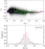 |
Fig. 12 Same as Fig. 11 for the (i − z) colours. |
| In the text | |
|
Fig. 13 Left: ESDLA BOSS spectrum (black) with the SDSS composite spectrum (grey) reddened by the SMC extinction-law at zabs(red) with E(B − V) = 0.02. The orange segments indicate the regions used for the fit. Right: distribution of E(B − V)-values for the corresponding control sample. In this example, the “zero-point” (respectively dispersion) of the distribution is −0.03 (respectively 0.044). The value retained for the DLA here is thus E(B − V) = 0.05 ± 0.05. |
| In the text | |
|
Fig. 14 Distribution of E(B − V) values (full sample as hashed histogram, subsample with Wr(Si iiλ1526) above (respectively below) 0.8 Å in red (respectively blue) unfilled histogram), fitted with Gaussian functions. The horizontal error bar in the upper left corner indicates the typical error on E(B − V), obtained from the standard deviation of the values in each control sample. |
| In the text | |
|
Fig. 15 Portion of the BOSS spectrum of SDSS J 113520−001053 in which the double peaked Ly α emission is clearly seen in the DLA trough. |
| In the text | |
|
Fig. 16 Results from spectral stacking. From left to right, the stacked spectrum corresponds to the median values, 3σ-clipped mean and weighted mean. The long red segment shows the DLA core region over which τ > 6 for log N(H i) ≥ 21.7, ensuring no residual flux from the quasar. This region is highlighted in the inset panels. The short red segment (inner tick marks) indicates the 1000 km s-1 central region over which the Ly α luminosity is integrated. The green spectrum is the composite Lyman-break galaxy spectrum from Shapley et al. (2003), scaled to match the same luminosity in the Ly α region. |
| In the text | |
|
Fig. 17 Results from bootstrapping: distribution of the measured mean Ly α luminosities using 300 random subsamples with half the size of the original sample. |
| In the text | |
|
Fig. 18 Distribution of Ly α luminosities estimated in individual ESDLAs (grey filled histogram). The blue hashed histogram represents the distribution after subtracting the mean luminosity observed on both sides of the Ly α region. The solid red curve represents the LAE luminosity function from Cassata et al. (2011) (arbitrary scaling), and the red unfilled histogram gives the expected distribution of L ≥ 1041 erg s-1 LAEs when Gaussian noise is added to mimic measurement uncertainties. |
| In the text | |
|
Fig. 19 Top: velocity offset of the Ly α profile compared to the systemic redshift. The black histogram shows the stacked ESDLA spectrum, the green line represents the LBG composite (Shapley et al. 2003, scaled down for illustration purposes) and the vertical blue line marks the typical velocity shift observed in LAEs (McLinden et al. 2011; Finkelstein et al. 2011; Hashimoto et al. 2013). Bottom: cross-correlation function obtained by correlating the Lyman-break galaxy and the ESDLA (3σ-clipped mean luminosity) composites at different velocities. The Ly α emission in the LBG composite is redshifted compared to that of ESDLAs by about 250 km s-1. The ESDLA Ly α emission redshift is much closer to the systemic redshift from the low-ionisation metal lines. . |
| In the text | |
|
Fig. 20 Effect of dust on the Ly α emission. The 3 σ-clipped mean luminosity are represented on the left panels and the corresponding bootstrap analysis on the right panels. The top (respectively bottom) panels correspond to the ESDLA subsample with E(B − V) < 0.025 (respectively E(B − V) ≥ 0.025). |
| In the text | |
|
Fig. 21 Normalised flux (black, 3 pixel boxcar smoothed) and error (orange) around the damped Ly α line. The Voigt-profile fit is overplotted in red, with the shaded area corresponding to an uncertainty of 0.2 dex. The QSO name, DLA resdshift and H i column density are indicated above each panel. |
| In the text | |
|
Fig. 21 continued. |
| In the text | |
Current usage metrics show cumulative count of Article Views (full-text article views including HTML views, PDF and ePub downloads, according to the available data) and Abstracts Views on Vision4Press platform.
Data correspond to usage on the plateform after 2015. The current usage metrics is available 48-96 hours after online publication and is updated daily on week days.
Initial download of the metrics may take a while.