| Issue |
A&A
Volume 566, June 2014
|
|
|---|---|---|
| Article Number | A122 | |
| Number of page(s) | 22 | |
| Section | Interstellar and circumstellar matter | |
| DOI | https://doi.org/10.1051/0004-6361/201321794 | |
| Published online | 24 June 2014 | |
The molecular complex associated with the Galactic H II region Sh2-90: a possible site of triggered star formation⋆
1 Aix-Marseille Université, CNRS, LAM (Laboratoire d’Astrophysique de Marseille) UMR 7326, 13388 Marseille, France
e-mail: This email address is being protected from spambots. You need JavaScript enabled to view it.
2 INAF – Instituto Fisica Spazio Interplanetario, via Fosso del Cavaliere 100, 00133 Roma, Italy
3 Department of Astronomy and Astrophysics, Tata Institute of Fundamental Research, Homi Bhabha Road, 400 005 Mumbai, India
4 Université de Toulouse, UPS-OMP, IRAP, 31 400 Toulouse, France
5 CNRS; IRAP ; 9 Av. du Colonel Roche, BP 44346, 31028 Toulouse Cedex 4, France
6 Aryabhatta Research Institute of Observational Sciences, 263 129 Nainital, India
Received: 29 April 2013
Accepted: 8 March 2014
Abstract
Aims. We investigate the star formation activity in the molecular complex associated with the Galactic H ii region Sh2-90.
Methods. We obtain the distribution of the ionized and cold neutral gas using radio-continuum and Herschel observations. We use near-infrared and Spitzer data to investigate the stellar content of the complex. We discuss the evolutionary status of embedded massive young stellar objects (MYSOs) using their spectral energy distribution.
Results. The Sh2-90 region presents a bubble morphology in the mid-infrared. Radio observations suggest it is an evolved H ii region with an electron density ~144 cm-3, emission measure ~ 6.7 × 104 cm-6 pc and an ionized mass ~55 M⊙. From Herschel and CO (J = 3 − 2) observations we found that the H ii region is part of an elongated extended molecular cloud (H2 column density ≥ 3 × 1021 cm-2 and dust temperature 18−27 K) of total mass ≥ 1 × 10⁴ M⊙. We identify the ionizing cluster of Sh2-90, the main exciting star being an O8–O9 V star. Five cold dust clumps, four mid-IR blobs around B stars, and a compact H ii region are found at the edge of the bubble. The velocity information derived from CO data cubes suggest that most of them are associated with the Sh2-90 region. One hundred and twenty-nine low mass (≤3 M⊙) YSOs have been identified, and they are found to be distributed mostly in the regions of high column density. Four candidate Class 0/I MYSOs have been found. We suggest that multi-generation star formation is present in the complex. From evidence of interaction, time scales involved, and evolutionary status of stellar/protostellar sources, we argue that the star formation at the edges of Sh2-90 might have been triggered. However, several young sources in this complex are probably formed by some other processes.
Key words: HII regions / stars: formation / stars: protostars
Full Table 5 is only available at the CDS via anonymous ftp to cdsarc.u-strasbg.fr (130.79.128.5) or via http://cdsarc.u-strasbg.fr/viz-bin/qcat?J/A+A/566/A122
© ESO, 2014
1. Introduction
There are several ways the energy inputs from the OB stars can modify the physical environment and chemistry of the host complex in which they reside (e.g., McKee & Ostriker 1977), and therefore can trigger the formation of a new generation of stars in the complex (e.g., Elmegreen & Lada 1977; Bertoldi & McKee 1990). Recent observational studies of bubbles associated with H ii regions (e.g., Deharveng et al. 2010), suggest that their expansion possibly triggers 14% to 30% of the star formation in our Galaxy (e.g., Deharveng et al. 2010; Thompson et al. 2012; Kendrew et al. 2012). These observational results have revealed the importance of OB stars on star formation activity on a Galactic scale. The detailed studies of individual objects (e.g., Deharveng et al. 2010; Urquhart et al. 2006; Zavagno et al. 2006, 2007), however, showed that the complex environments around H ii regions makes determining the exact process of star formation difficult and that, in general, this process is complicated.
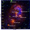 |
Fig. 1 Color-composite image of the Sh2-90 complex. Spitzer-IRAC 8.0 μm (red) and 3.6 μm (green) images have been combined with the DSS2 R-band (blue) image. The different sources associated with the region (see the text) are marked. The field size is 12 |
Now the far-infrared (FIR) observations provided by Hi-GAL (Herschel Infrared Galactic Plane Survey; Molinari et al. 2010a) using the Herschel Space Observatory have the ability to image a large area of a cloud complex with unprecedented sensitivity, thus allowing us to improve our understanding of how OB stars interact with the local interstellar medium (ISM), and process cold gas to induce new star formation. The recent studies based on Herschel observations revealed that star-forming regions (SFRs) are composed of very complex and filamentary clouds, with ongoing star formation at various locations (e.g., Hill et al. 2011; Giannini et al. 2012; Hennemann et al. 2012; Deharveng et al. 2012; Schneider et al. 2012; Preibisch et al. 2012; Roccatagliata et al. 2013). Demonstrating the existence of triggered star formation in extended clumpy clouds by internal feedback sources is difficult, because they may be forming new stars in various ways. For example, such clouds can form stars spontaneously governed by the physical condition and the evolution of the original cloud or the collapse of high-density structures generated by the large-scale supersonic turbulence of the the ISM (e.g., Mac Low & Klessen 2004). Thus, understanding of the physical connection and interaction of bubbles/H ii regions with the cold ISM, and their association with stellar/protostellar content is central to obtaining a better picture of star formation around H ii regions. In this context, we present here a multiwavelength investigation of the Sh2-90 H ii complex (briefly described in Sect. 2) in order to decipher its star formation activity.
In the present work, we analysed the distributions of the ionized and cold neutral ISM, with radio continuum observations at low frequencies (610 and 1280 MHz) and dust continuum emission with Herschel in the wavelength range 70−500 μm. We explore the stellar and proto-stellar components of the complex, using high-resolution JHK observations coupled with archival Spitzer-IRAC observations. We have organized this work as follows. Section 2 presents the Galactic H ii region Sh2-90. In Sect. 3, we describe the observations and the reduction procedures. Section 4 describes the H ii region (adopted distance, general morphology, properties of ionizing gas, and exciting source). Section 5 deals with the distribution and physical condition of the cold ISM, and the properties of compact dusty clumps. In Sect. 6, we describe the identification and classification of young stellar objects (YSOs), their nature and distribution. The kinematics of ionized and molecular gas is presented in Sect. 7. Section 8 is devoted to the general discussion and our understanding of star formation in the Sh2-90 complex. We present the main conclusions in Sect. 9.
IRAS point sources towards the Sh2-90 complex.
2. Description of the Sh2-90 complex
The Sh2-90 complex (Sharpless 1959), located at α2000 = 19h49m11s, δ2000 = + 26°51′36′′ ( ,
,  ), is an optically visible irregularly shaped H ii region. This H ii region is a part of the Vulpecula OB association (Turner 1986). The most commonly adopted distances to the H ii region are between 1.6 kpc and 2.5 kpc (Stark 1984; Beaumont & Williams 2010; Russeil et al. 2011). We discuss the distance in Sect. 4 and adopt a value of 2.3 kpc in the present study. The main exciting source of the nebula is uncertain; measurements based on an indirect approach suggest that it has been created by a star of O9.5V–O8V spectral type (Georgelin et al. 1975; Lafon et al. 1983). Observations in the 13CO (110.201 GHz) and HCO+ (89.189 GHz) lines suggest that Sh2-90 is a part of a massive (~ 4 × 10⁴ M⊙) asymmetric cloud (Lafon et al. 1983).
The Sh2-90 molecular cloud complex contains several kinds of sources. Figure 1 displays the color-composite image made with the R-band (DSS2 survey) in blue, the emission at 3.6 μm in green and the 8.0 μm emission in red (Spitzer-GLIMPSE survey; see Sect. 3.3). The various sources discussed in the present work are marked in Fig. 1. The sources N133 and N132 are identified as bubbles in the Spitzer 8.0 μm band (Churchwell et al. 2006) of the GLIMPSE survey. Of the two bubbles, N133 is an elliptical bubble of average radius ~1 6, which encloses the H ii region Sh2-90, while N132 is a circular bubble of average radius ~028; N133 is associated with a detectable radio H ii region (Israel 1977), but no radio emission has been reported in the direction of N132. Several IRAS sources (see Table 1) are identified in close proximity to Sh2-90. The fluxes of these IRAS sources at 12, 25, 60, and 100 μm have been taken from the IRAS Catalog of Point Sources, Version 2.0 (Helou & Walker 1988). We estimated the FIR luminosity (see Table 1) of these IRAS sources from the IRAS fluxes using the relation given in Casoli et al. (1986). The source IRAS 19473+2638 (luminosity ~ 5.7 × 10³ L⊙) is located in the close vicinity of N132, whereas IRAS 19474+2637 (luminosity ~ 1.0 × 10⁴ L⊙) is located ~23 S-E of N132. The location of IRAS 19473+2647 is about ~50 N-E of N133, and is a low luminosity (~ 0.3 × 10³ L⊙) source.
Apart from the above distinct IRAS sources, close to Sh2-90 and at its southern edge lies the IRAS source 19474+2641 of luminosity ~ 7.7 × 10³ L⊙. Another IRAS source 19470+2643 of luminosity ~ 7.6 × 10³ L⊙ is situated at the western edge of Sh2-90. Figure 1 also shows two compact symmetric 8.0 μm dust emissions at the eastern side of Sh2-90. These symmetric 8.0 μm structures coincide with the MSX point sources (Egan et al. 2003) G063.1549+00.4309 and G063.1422+00.4227. The colors (F21/F8 and F14/F12) of these sources at MSX bands (8.28 μm (A), 12.13 μm (C), 14.65 μm (D), and 21.34 μm (E)) fall in the criteria of a compact H ii region developed by Lumsden et al. (2002), who used these colors to identify various sources in the Galactic Plane. Altogether, the Sh2-90 region has a bubble morphology with minimal 8 μm emission at its center, and is surrounded by several luminous infrared (IR) sources. These configurations are possible sites of a new generation induce star formation (e.g., Deharveng et al. 2005; Zavagno et al. 2007; Samal et al. 2012). Thus, the Sh2-90 complex is a potential target for examining the influence of an H ii region on star formation processes.
3. Observations and data reduction
3.1. Optical photometry
The optical photometric observations at the V and I bands were performed for the Sh2-90 region (centered on α2000 = 19h49m29s, δ2000 = + 26°50′13′′) on 2006 June 02, using the 2K × 2K CCD system of the 104 cm Sampurnanand Telescope, Nainital (India). The 0.37 arcsec pixel-1 plate scale gives a field of view (FoV) of  ×
×  on the sky. To improve the signal-to-noise ratio (S/N), the observations were carried out in binning mode of 2 × 2 pixels. The observing conditions were photometric and the average FWHM during the observing period was ~1
 7–20. The initial processing and photometry of the images were done using IRAF. We used the point spread function (PSF) algorithm ALLSTAR in the DAOPHOT package to extract the photometric magnitudes. The PSF was determined from the bright and isolated stars of the field. The calibration from instrumental to standard system was done using the procedure outlined by Stetson (1987), using the standard field SA101 (Landolt 1992) observed during the same night. The standardization residuals between the standard and transformed V and I magnitudes and colors were less than 0.05 mag. Stars having photometric error ≤ 0.1 mag are used in the present analyses.
Completeness limits of the observations were calculated quantitatively by plotting histograms of the point sources, and we considered that the data is complete up to the linear distribution in the histograms. With this approach the approximate completeness limits for the V- and I-band data are 18.0 mag and 18.5 mag, respectively.
3.2. CFHT near-infrared imaging
Deep NIR observations of the Sh2-90 region (centered on α2000 = 19h49m18s, δ2000 = + 26°48′46′′) in the J (λ = 1.25 μm), H (λ = 1.63 μm), and Ks (λ = 2.14 μm) bands were obtained on 2006 July 06 with the WIRCAM camera of the CFHT 3.6 m telescope (Puget et al. 2004). In this set up, each pixel corresponds to 03 and yields a FoV ~ 200 × 200 on the sky. The observing conditions were photometric and the average FWHM during the observing period was ~07–09. The initial processing of the data was done in the CFHT pipeline software TERAPIX (Bertin & Arnouts 1996). We perform photometry for an area of ~125 × 125 centered on α2000 = 19h49m18s, δ2000 = + 26°49′29′′. Photometry on the images was done using the PSF algorithm of DAOPHOT package (Stetson 1987) in IRAF. The PSF was determined from the bright and isolated stars of the field. For photometric calibration, we used isolated Two Micron All Sky Survey (2MASS) point sources (Cutri et al. 2003) having error <0.1 mag and rd-flag “123”. Rd-flag values of 1, 2 or 3 generally indicate the best quality detections, photometry, and astrometry. A mean calibration dispersion ≤0.06 mag is observed in each band, indicating that our photometry is reliable within ~0.06 mag; 290 sources were found to be saturated in our catalog; these sources were replaced by 2MASS sources. Sources with photometric error ≤ 0.1 mag in all the three bands are considered in the present work.
To evaluate the completeness of the census of JHK detection quantitatively, we plot histograms of the JHK point sources and considered the data is complete up to the linear distribution in the histograms (e.g., Ohlendorf et al. 2013). In this way the completeness limits for the J-, H-, and K-band data are ~19, 18, and 17 mag, respectively.
3.3. Spitzer observations and point source catalogs
The Sh2-90 complex was observed as part of the Galactic Legacy Infrared Mid-Plane Survey Extraordinaire (GLIMPSE; Benjamin et al. 2003, PI: E. Churchwell; Program ID: 188) and the Multiband Imaging Photometer GALactic plane survey (MIPSGAL; Carey et al. 2009, PI: S. Carey; Program ID: 20597) by Spitzer Space Telescope. We downloaded the Post Basic Calibrated Data (PBCD) images of the Spitzer Infrared Array Camera (IRAC) at 3.6, 4.5, 5.8, and 8.0 μm, and Multiband Imaging Photometer (MIPS) 24.0 μm PBCD images from the Spitzer Archive1 to study the morphology of the complex. The angular resolution of the images at IRAC bands are <2.̋0, whereas it is ~6.̋0 at the MIPS 24 μm band.
For the point source analyses, we used the GLIMPSE point source catalog available on the Vizier website2. Applying the same procedure as described in Sect. 3.2, we quantitatively considered that the IRAC point source catalog is nearly complete down to 13.5, 13.5, 12.0, and 11.0 mag at 3.6, 4.5, 5.8, and 8.0 μm bands, respectively.
3.4. Herschel multi-band observations in the range 70–500 μm
The FIR data used in this paper were taken with the Herschel-PACS (Poglitsch et al. 2010) and SPIRE (Griffin et al. 2010) imaging cameras as part of the Hi-GAL survey. This survey is a Herschel Open Time key project that maps the whole Galactic Plane in five bands centered at 70 μm and 160 μm with PACS, and 250 μm, 350 μm, and 500 μm with SPIRE (Molinari et al. 2010a,b). The spatial resolutions of these bands are 67, 110, 180, 250, and 370, respectively. At the distance of the Sh2-90 complex, this corresponds to a physical scale in the range 0.07−0.41 pc. The data are acquired in PACS/SPIRE Parallel mode by moving the satellite at a constant speed of 600/s and acquiring images simultaneously in the five photometric bands. The detailed description of the observation settings and scanning strategy adopted is given in Molinari et al. (2010b). The detailed description of the pre-processing of the data up to usable high-quality maps can be found in Traficante et al. (2011).
3.5. Radio continuum mapping
The radio continuum interferometric observations of the Sh2-90 region (centered on α2000 = 19h49m18s, δ2000 = + 26°53′12′′) at 1280 MHz and 610 MHz were carried out on 2007 December 22 and 2007 December 28, respectively, using the Giant Metrewave Radio Telescope (GMRT) array (Swarup et al. 1991). The sources 3C 48 and 3C 286, and 1924+334 were observed as flux and phase calibrators to derive the phase and amplitude gains. The NRAO Astronomical Image Processing System (AIPS) was used for the data reduction. While calibrating the data, the data were carefully checked and bad data points were flagged at various stages. The estimated uncertainty of the flux calibration was within 8% at both frequencies. The image of the field was formed by Fourier inversion and the cleaning algorithm task IMAGR. The resulting images at 1280 MHz (beam ~16′′× 11′′, rms noise ~1.2 mJy/beam) and at 610 MHz (beam ~34′′× 22′′, rms noise ~7 mJy/beam) were made with a Brigg’s weighting function (robust factor 0). At the distance of the Sh2-90 complex, the mean beam width of the radio images corresponds to a physical scale in the range 0.15–0.31 pc. Few iterations of self-calibration were carried out to remove the residual effects of atmospheric and ionospheric phase corruptions and to obtain improved maps. The system temperature correction was done using sky temperature from the 408 MHz map of Haslam et al. (1982). A correction factor equal to the ratio of the system temperature toward the source and flux calibrator has been used to scale the images.
For the Sh2-90 complex, different observations with different areas have been conducted or taken from the archive, but in the following we have done the point source analyses for a common area of ~12′ × 12′ centered on α2000 = 19h49m18s, δ2000 = + 26°49′29′′ (i.e., the area of Fig. 1).
Kinematic information of the Sh2-90 complex.
4. Distance, morphology, and nature of the ionized gas
The distance of the region is uncertain and different indicators suggest a near kinematic distance in the range of 1.6−2.5 kpc (for discussion, see Lafon et al. 1983; Beaumont & Williams 2010; Russeil et al. 2011).
The mean velocities of the molecular gas observed towards the Sh2-90 H ii region (l = 63.̊10, b = +0.̊46) are given in Table 2. Table 2 shows that the molecular emission towards the region is mainly in the velocity range 20.5−22.2 km s-1. Using the Galactic rotation curve of Brand & Blitz (1993), this velocity range corresponds to a near kinematic distance in the range 2.1−2.4 kpc.
Lafon et al. (1983), based on the [Oiii/Hβ] strength, suggested that the main exciting source of Sh2-90 is a star of spectral type O8–O9. We identify the exciting source at the center of the nebula (see Sect. 4.3). Using its near-infrared magnitude and colors (J = 11.00, J − H = 0.99 and J − K = 1.46), the synthetic photometry of O stars by Martins & Plez (2006), and the interstellar extinction law of Rieke & Lebofsky (1985), we estimated a distance of 2.5 kpc for an O8V star and 2.2 kpc for an O9V star.
From the above analyses it appears that the distance of Sh2-90 lies in the range of 2.1−2.5 kpc. In the following, we thus adopted a mean distance of 2.3 ± 0.2 kpc. From our radio observations, with this distance, we derived the Lyman continuum photons emanating from the associated massive star of the region (see Sect. 4.2), which is compatible with an O8–O9 star. This further supports the distance of 2.3 kpc for the region. We note that at this distance an angular size 1.̋0 corresponds to a physical size ≃0.01 pc on the sky.
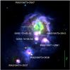 |
Fig. 2 Color-composite image of the Sh2-90 complex centered at α2000 = 19h49m17.5s, δ2000 = + 26°49′55′′. Herschel-PACS 70.0 μm (red), have been combined with Spitzer-MIPS 24.0 μm (green) and Spitzer-IRAC 8.0 μm (blue) images. The arrow points to the 24.0 μm circular structure. North is up and east is to the left. |
4.1. Infrared and radio view of the complex
Figure 1 shows the morphology of the complex in optical (R-band) and IR (at 3.6 μm and 8.0 μm) bands. The 8.0 μm emission displays a central cavity surrounded by a roughly thin annular shell emission. The 8.0 μm IRAC band contains emission bands at 7.7 μm and 8.6 μm, commonly attributed to polycyclic aromatic hydrocarbon (PAH) molecules; PAHs are believed to be destroyed in the ionized gas (Pavlyuchenkov et al. 2013), but are thought to be excited in the photo-dissociation region (PDR) at the interface of the H ii region and molecular cloud by the absorption of far-UV photons from the exciting stars of the H ii regions. The 8.0 μm IRAC diffuse emission is extended, well beyond the main shell, possibly because of the leakage of UV photons through holes into the neutral material. The emission at the 3.6 μm band is mostly from stellar sources, but this band also has contributions from a weak, diffuse PAH feature at 3.3 μm. Figure 2 displays the color-composite image made with the Spitzer-IRAC 8.0 μm emission in blue, the Spitzer-MIPS 24.0 μm emission in green, and the Herschel-PACS 70.0 μm emission in red. Leaving the mid-IR (MIR) emission from stellar and proto-stellar sources aside, the brightness distribution of the diffuse 24 μm emission differs from that of the diffuse 8.0 μm emission. The 24 μm emission is bright in the direction of the center of the H ii region, a region devoid of PAHs emission. As shown by the radiative transfer model of Pavlyuchenkov et al. (2013) this emission comes from very small dust grains (VSGs; a few nm in size) located inside the ionized region, and out of thermal equilibrium after absorption of ionizing photons. Diffuse 24 μm emission is also observed in the direction of the neutral PDR surrounding the ionized region. Most of the diffuse 70 μm emission also comes from the PDR. Compiègne et al. (2010) have shown that stochastically heated VSG components can contribute significantly (up to 50%) to the diffuse emission at 70 μm.
Figure 2 also displays bright compact dust structures at the locations of MSX and IRAS sources. It also shows one roughly circular 24 μm emission structure (pointed with an arrow), which lies close to a 250 μm clump (discussed in Sect. 6.4). These IR compact structures possibly represent the heated dust around embedded massive source(s). We shall refer to the 24 μm structure, the two MSX sources (G063.1549+00.4309 and G063.1422+00.4227), and the IRAS source IRAS 19471+2641, as IR1, (IR2 and IR3), and IR4, respectively, in the text wherever necessary. We discuss these dusty structures in Sect. 6.4.
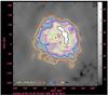 |
Fig. 3 Radio continuum map of Sh2-90 at 1280 MHz. The contour levels are at 1.20 × (4.5, 6, 8, 10, 14, 20, 28, 38) mJy beam-1, where 1.21 mJy beam-1 is the rms noise of the 1280 MHz map. North is up and east is to the left. |
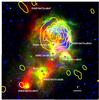 |
Fig. 4 Color-composite image of the Sh2-90 complex centered at α2000 = 19h49m18s, δ2000 = + 26°49′29′′. Herschel-SPIRE 350.0 μm (red), has been combined with Spitzer-IRAC 8.0 μm (green) and DSS2 R-band (blue) images. The radio continuum 610 MHz contours are overplotted with yellow lines. The contour levels are at 7 × (3, 5, 9, 13) mJy beam-1, where ~7 mJy beam-1 is the rms noise of 610 MHz map. North is up and east is to the left. |
Figure 3 shows the radio continuum view of the Sh2-90 H ii region at 23 cm. This high-resolution (beam ~160 × 110) map shows the non-uniform distribution of the ionized gas. The complex structure of the radio emission suggests that it could be due to density inhomogeneities within the H ii region. Our high-resolution 23 cm image allows us to identify a compact (diameter 0.6 pc) radio emission (at α2000 = 19h49m09s, δ2000 = + 26°48′60′′) at the S-W edge of Sh2-90. The position of this compact radio source coincides with the location of IRAS 19471+2641.
Figure 4 shows the color-composite image in the R-band (blue), 8.0 μm (green), and 350 μm (red), overplotted with radio contours at 50 cm. The 50 cm image comprises a cometary head in the N-W direction and an intensity gradient towards the S-E direction (see Fig. 4). In Fig. 4, the H ii region shows complex morphology in the optical, with diffuse, patchy, and irregular extended emission. An absorption lane in the optical band is clearly seen at the center of the nebula, which is more prominent from the center to the N-E direction. The optical image and radio contours display different morphology at smaller scale. The N-W part of the nebula is bright in both the images. The striking difference in Fig. 4 is the strong radio emission at the center and easternside of the nebula, corresponding to the zone of optical absorption. This indicates that the optical emission is absorbed by a dust cloud along the line of sight. We observed cold neutral material, prominent at longer wavelengths (≥350 μm), and distributed along an elongated structure which extends from the center to the N-E and S-E directions. This implies that the cold gas is in front of the H ii region. We note that although our low resolution 610 MHz map shows the extended H ii region well, we do not see the compact radio source at the 3σ upper limit level (i.e., ~21 mJy). The non-detection of the compact radio source could be due to the fact that it is optically thick at 610 MHz. High-resolution sensitive low-frequency maps would shed more light on the nature of this source.
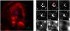 |
Fig. 5 Left: 8.0 μm image (red; from Spitzer-IRAC) centered at α2000 = 19h49m13s, δ2000 = + 26°50′42′′, showing structures pointing to the exciting star candidates shown in R-band image (blue: from DSS2). Right: images showing the exciting star candidates (marked with 1, 2, 3, and 4) at various wavelengths in the range 0.54 to 24 μm (i.e., images at V, I, J, K, 3.6 μm, 4.5 μm, 5.8 μm, 8.0 μm, and 24 μm bands). |
4.2. Properties of the ionized gas
The flux densities (Sν) of Sh2-90, estimated by integrating over 4σ contours yield S23 cm = 5.03 ± 0.5 Jy and S50 cm = 3.20 ± 0.3 Jy, where σ is the rms noise of the respective radio images. Our 23 cm flux density within uncertainty is close to the flux densities at 21 cm (5.8 ± 0.7 Jy) and 6 cm (5.0 ± 1.0 Jy) measured by Israel (1977). The flux densities at 23 cm, 21 cm, and 6 cm reflect a flat spectrum, indicating the region is optically thin at 23 cm. Figure 3 shows that the radio emitting region is almost circular in shape and has a diameter about 48 (or 3.3 pc at 2.3 kpc). Using the 23 cm flux density and assuming a spherically symmetric, optically thin homogeneous nebula, we determine the physical conditions and properties of the ionized gas following the prescription given in Kurtz et al. (1994, and references therein). Considering 7370 K as the electron temperature (Te; Quireza et al. 2006) of the ionized gas, we derived parameters such as the total number of Lyman continuum photons per second (NLyc ~ 22.5 × 1047 s-1) coming from the associated massive star(s), the rms electron density (ne ~ 144 cm-3), the emission measure (EM ~ 6.7 × 104 cm-6 pc), and the mass of the ionized gas (Mion ~ 55 M⊙) for Sh2-90. The estimated NLyc (log (NLyc) ≃ 48.35), suggests that the spectral type of the ionizing source responsible for the ionization of Sh2-90 is an O8–O9V star according to Smith et al. (2002), or an O8–O8.5V star according to Martins et al. (2005). Because of our limited knowledge on the dust absorption of Lyc photons and clumpy nature of the medium, the estimated NLyc could be on the lower side. The flux density of the compact H ii region is ~0.04 Jy. Assuming that the compact H ii region associated with IRAS 19471+2641 is optically thin at 1280 MHz, we estimated NLyc as ~ 1.4 × 1046 s-1 for an electron temperature ~10 000 K, which is equivalent to the Lyman continuum photons coming from a star of spectral type B1 V (Smith et al. 2002).
Photometric magnitudes of candidate ionizing stars.
4.3. Ionizing source(s) of Sh2-90
The exciting star of Sh2-90 has not been clearly identified. According to Georgelin et al. (1975), the exciting star of Sh2-90 is an O9.5 III (ALS 10542; V = 11.41 mag and B − V = 0.78 mag) star, located at α2000 = 19h49m14s, δ2000 = + 26°47′39′′, thus ~35 north of Sh2-90, i.e., significantly off center. Lafon et al. (1983), based on the observed [Oiii/Hβ] line ratio (by Chopinet & Lortet-Zuckermann 1976), suggested that the ionizing star should be of spectral type O8–O9 V, and more likely located inside the Sh2-90 region. In agreement with Lafon et al. (1983), our support for the exciting star being inside the bubble are as follows:
-
At 8.0 μm, the region shows a cavity at its center, surrounded by PAH emission in the PDR (see Fig. 1).
-
The 24 μm diffuse emission is strongest in the center of the nebula (see Fig. 2), implying that the dust heating source might be at the center of the nebula. This phenomenon has been observed in many bubbles associated with H ii regions (e.g., Deharveng et al. 2010).
-
Generally, the radio free-free emission comes from the immediate vicinity of the OB stars in young H ii regions (see Fig. 4).
All this evidence suggests that the exciting star(s) must be located inside the bubble. Thus, we searched for the exciting star(s) of the bubble within the dust cavity. First, we identified all the luminous sources inside the bubble earlier than B2V stars. We followed the same prescription as described in Samal et al. (2010), of rejecting the most-likely giants and foreground sources based on J vs. J − H and J − H vs. H − K diagrams. After these eliminations we remain with a massive O-type star located at the center of the bubble close to the strong 24 μm emission. This source is associated with a group of stars in its close vicinity, possibly part of an exciting cluster (Fig. 5, left). The images of the ionizing candidates at various wavebands in the range 0.54−24 μm are shown in Fig. 5 (right). In optical bands only four sources are visible; their coordinates and fluxes at various wavelengths are given in Table 3. Our high-resolution deep NIR images, however, reveal many faint sources, suggesting the presence of a small cluster. The fainter sources disappear at IRAC-MIPS wavelengths possibly because of a combined effect of lower sensitivity and poor resolution of IRAC-MIPS bands.
Out of four sources, source 2 (J = 11.00 mag, J − H = 0.99 mag) is the most luminous one. We assume that star 2 is an O8–O9 MS star (using the prediction by Lafon et al. 1983); using its NIR photometry and synthetic colors of O stars by Martins & Plez (2006), its visual extinction is ~10 mag (using the extinction law of Rieke & Lebofsky 1985). Using the above extinction value, the observed J magnitude of the star and MJ-spectral type calibration table of Martins & Plez (2006), we estimated that the distance to the star is in the range of 2.2−2.5 kpc. This distance range is in agreement with the kinematic distance 2.1−2.4 kpc.
Adopting the distance of Sh2-90 in the range of 2.1−2.5 kpc, source 3 (J = 12.47 mag, J − H = 0.84 mag) is consistent with a B2–B3 star, whereas the nature of the other two neighboring sources, star 1 (J = 13.92 mag, J − H = 0.54 mag) and star 4 (J = 14.32 mag, J − H = 0.54 mag) appear to be low-mass stars. From the above discussion, we conclude that source 2 is the most-likely ionizing star of Sh2-90.
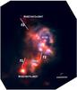 |
Fig. 6 Color-composite image of the Sh2-90 complex at Herschel 350 μm (red), 160 μm (green), and 70 μm (blue) bands centered at α2000 = 19h49m20s, δ2000 = + 26°50′09′′. The positions of the main star-forming sites are also marked (see Fig. 1). The solid lines represent the small filament-like structures (marked as f1, f2, and f3) of the region. North is up and east is to the left. |
5. Distribution of cold neutral material in the complex
5.1. Dust continuum distribution
Recent Herschel observations have shown that SFRs are interconnected with network of filamentary structures (e.g., Arzoumanian et al. 2011), and that the massive-star-forming sites are often associated with the main filament of the complex. In Fig. 6, we present a color-composite image of the Sh2-90 complex at 350 μm (red), 160 μm (green), and 70 μm (blue). Because of the low resolution of the images, the individual components or cavities seen at 8.0 μm (Fig. 1) are not clearly distinguishable at 160 μm and 350 μm, but the complex is more extended at Herschel-SPIRE wavelength than at 8 μm, showing new structures such as small filaments f1, f2, f3 (~0.7−1.3 pc in length and ~0.3−0.4 pc in width) at the outer extent of Sh2-90. The fact that these filaments are not observed at 70 μm tells us that they are possibly far away from any source of strong radiation. Filament-like structures are often considered as the possible sites of on-going or future star formation.
5.2. Physical conditions of the cold ISM
Thermal emission from dust can be used to determine the physical conditions of a cloud such as temperature, density, and mass. We derived the cold dust temperature using the Herschel fluxes. We convolved all the Herschel maps to the 500 μm band resolution, then all the maps are re-gridded to the pixel size of the 500 μm map. We then subtracted a background flux (i.e., 14, 19, 18, 15, and 13 Jy/pix at 70, 160, 250, 350, and 500 μm, respectively), to minimize the contribution of excess emission along the line of sight. The background area was chosen far from the main cloud complex. We fit a modified blackbody of single temperature to the observed fluxes on pixel by pixel basis to construct the temperature map.
We used a dust spectral index of β = 2, and dust opacity law as given in Deharveng et al. (2012), in which the dust opacity per unit mass column density (κν) is κν = 10 (ν/ 1000 GHz)β cm2/g. The choice to use the present opacity law and its limitation have been discussed in Deharveng et al. (2012). We adopted β = 2, because this is close to the value found in H ii environments (e.g., Anderson et al. 2012). During the spectral fitting, we iteratively applied color correction factors by repeatedly fitting a temperature, and then applying the corresponding correction factors until successive fit results were unchanged. We used the color corrections given in PACS calibration release note “PACS Photometer Pass-bands and Color Correction Factors for Various Source SEDs”. The color-corrected temperatures are higher than those obtained without corrections by about 0.2 K to 0.7 K, with a median difference of ~0.4 K. From the temperature map, we then derived the H2 gas column density map using the dust continuum emission at 500 μm, gas-to-dust ratio R = 100, and 2.8 as the mean molecular weight per H2 molecule.
We derive the dust properties excluding and including 70 μm emission in the spectral fitting procedure. It has been demonstrated that a non-negligible fraction of the 70 μm emission comes from stochastically heated very small grains (e.g., Compiègne et al. 2010; Pavlyuchenkov et al. 2013); this is especially true when an H ii region is present along the line of sight. In consequence, we prefer to consider the dust emission in the range from 160 μm to 500 μm. Figure 7 shows the dust maps that were obtained excluding 70 μm emission in the spectral fitting procedure. However, we also explored the dust properties including 70 μm emission in the spectral fitting. The inclusion of the 70 μm emission results in a temperature higher by a few kelvin for the whole complex. In the following, while considering a specific structure we discuss the physical properties using the two temperatures (the physical properties that are obtained from including the 70 μm flux in the spectral fitting are given in the brackets). We note that if the anti-correlation between the dust temperature and the spectral index (i.e.,  ; Anderson et al. 2012) is valid, then the temperature of the cold regions (e.g., <15 K) in our map should be considered as an upper limit, and for warm regions (e.g., >30 K) it should be treated as a lower limit. The average temperature of the Sh2-90 complex is about 18.5 K (21.5 K); higher temperatures are found in PDRs and in some of the clumps. The temperature of the PDR associated with N133 is in the range of 22−24 K (23.5−27.5 K), whereas the temperature of N132 is around 20 K (22.7 K). The PDR at the western side of Sh2-90 has a higher temperature and a lower column density than that of its eastern edge, reflecting the presence of warmer material at the western periphery of Sh2-90. The Sh2-90 complex also contains a number of cool filament-like structures (see Fig. 6). The temperatures in their directions lie in the range of 14−17 K (14.5−18 K). The column density map shows roughly an elongated interconnected distribution of high column density (> 6.4 × 1021 cm-2; white contour in Fig. 7, bottom) material, broadly running from S-E to N-W then towards N-E via Sh2-90, with local maxima (>1022 cm-2; cyan contour in Fig. 7, bottom) at five locations.
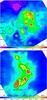 |
Fig. 7 Top: dust temperature map of the Sh2-90 complex centered at α2000 = 19h49m21s, δ2000 = + 26°50′18′′. The horizontal color bar is labeled in units of kelvin (K) and the contours are at 14.6 K (yellow), 18 K (red), 19 K (blue) and 23 K (black). The map was obtained by fitting the dust emission between 160 μm and 500 μm. Bottom: H2 column density map of the same region. The horizontal color bar is labeled in units of cm-2 and the contours are at 3.3 (yellow), 6.4 (white), 9.3 (black), 12 (cyan), 16 (blue) and 32 (green) × 1021 cm-2. North is up and east is to the left. The labeled axes are in J2000 coordinates. The plus symbols represent the locations of the IR sources shown in Fig. 1. |
The regions of high column density correspond to low temperature zones and vice versa. The column density is highest in the direction of IRAS 19474+2637, reaching a value of ~ 4.5(3.4) × 1022 cm-2.
The column density map can be used to estimate the total mass of the cloud using the relation:  (1)where mH is the hydrogen mass, A is the pixel area in cm-2, and μH2 is the mean molecular weight per H2 molecule. To estimate the mass of the cloud, we integrated over all the pixels in the column density map having a value ≥ 3.3 × 1021 cm-2 (yellow contour in Fig. 7, bottom). This value corresponds to four times the background column density value on the map. The resulting mass of the cloud is ~ 1.6 × 10⁴M⊙. This value is lower by 20% when derived from the column density map that uses a 70 μm flux in the process of spectral fitting. These values are compatible with the mass ~ 4 × 10⁴M⊙ derived by Lafon et al. (1983) using CO observations. It seems that the Sh2-90 H ii region was born in a massive cloud of mass ~ 104M⊙ or greater.
Physical properties of the clumps.
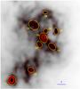 |
Fig. 8 250 μm cold dust emission contours superimposed on the 250 μm image. The image is centered at α2000 = 19h49m16s, δ2000 = + 26°49′39′′. The contour levels are in the range from 980 MJy sr-1 to 3000 MJy sr-1 at intervals of 199 MJy sr-1. North is up and east is to the left. The clumps discussed in the text are labeled C1 to C9. The yellow ellipses are the apertures used to integrate the 250 μm fluxes. |
5.3. Dust continuum clumps and accumulated neutral matter
Figure 8 shows the 250 μm emission contours of the complex. The 250 μm emission map reveals nine compact structures associated with the main star-forming sites, and are marked in the figure. To estimate the mass of these compact structures, we integrated their 250 μm fluxes above the local background using elliptical apertures. Since the clumps are part of interconnected extended structures, a clear boundary cannot be assigned to them. We chose aperture (boundary) such that it closely encloses the flux within the outer contour level, and separated the clumps from the extended structures to make them as single entities (see Fig. 8). Since we need to know the temperature to estimate the mass, we measured the average temperature of each compact structure from the temperature maps using the same elliptical aperture that was used for the flux estimation. We also subtracted background flux from each clump to minimize the excess emission along the line of sight plus the contribution of the diffuse cloud in which they are embedded. The background areas were chosen close to each compact structure; however, since the background level is non-uniform even on a small scale, its accurate measurement is always problematic, which adds an extra uncertainty in the real flux estimations of the compact structures. Keeping all these uncertainties in mind, we derived the mass (gas + dust) of the compact structures using the relation (derived from Hildebrand 1983) for optically thin emission, 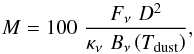 (2)where Fν is the measured integrated flux density, D is the distance of the source, κν is the dust opacity per unit mass at frequency ν (see Sect. 5.2), and Bν(Tdust) is the Planck function for a dust temperature Tdust. We have assumed a gas-to-dust ratio of 100. A requisite of this formulation is that the compact structures should be optically thin at the adopted frequency. Assuming the same kind of dust discussed in Sect. 5.2, an optical depth ~1 at 250 μm corresponds to a column density value ~ 1.5 × 1024 cm-2. The maximum column density (i.e., ~4.5(3.4) × 1022 cm-2; see Sect. 5.2) found in the direction of Sh2-90 is significantly lower than the value ~ 1.5 × 1024 cm-2; thus, we considered that all our compact structures are optically thin at 250 μm.
We give the peak position, integrated flux density at 250 μm (F250), mean diameter (d; the geometric mean of semi-major and semi-minor axes of ellipse), measured dust temperature (Tdust), mass (M), and density (nH2) of each compact structure in Table 4. We note nH2 has been estimated assuming a uniform density inside the aperture. Bergin & Tafalla (2007) defined a clump as having a size 0.3−3 pc and containing mass 50−500 M⊙ and defined a core as size being around 0.03−0.2 pc and having a mass of 0.5−5 M⊙. We observed that the size, mass, and density of the clumps are in the range 0.3−0.6 pc, 10(8)−206(186) M⊙, and 0.5(0.4)−1.8(1.7) × 104 cm-3, respectively. Here again the values in brackets are obtained including the 70 μm emission in the temperature determination. Following the nomenclature used by Bergin & Tafalla (2007), in the following we refer to these compact structures simply as clumps.
To test whether these clumps are gravitationally bound entities or if some of them are unbound transient structures, we estimated the Bonnor-Ebert critical mass (MBE) using the following relation from Lada et al. (2008): ![Mathematical equation: \begin{eqnarray*} M_\mathrm{BE} \sim 1.82 \left(\frac{n_{\mathrm{H}_2}}{\left[10^4\right]~{\rm cm^{-3}}}\right)^{-1/2} \left(\frac{T}{[10]~{\rm K}}\right)^{3/2}~\msun. \end{eqnarray*}](/articles/aa/full_html/2014/06/aa21794-13/aa21794-13-eq153.png) Within the framework of this simple approach, the clump with mass greater than MBE will collapse under the effect of self-gravity in the absence of other forces, whereas the clump with mass less than MBE is not gravitationally bound or unstable. To derive MBE, we used the temperature and density given in Table 4. The results are such that all the clumps seem to be gravitationally bound and so can lead to star formation, except clumps C8 and C9, which are marginally bound.
Within the framework of this simple approach, the clump with mass greater than MBE will collapse under the effect of self-gravity in the absence of other forces, whereas the clump with mass less than MBE is not gravitationally bound or unstable. To derive MBE, we used the temperature and density given in Table 4. The results are such that all the clumps seem to be gravitationally bound and so can lead to star formation, except clumps C8 and C9, which are marginally bound.
Kauffmann & Pillai (2010) suggested an approximate threshold for massive star (M> 10 M⊙) formation by comparing clouds with and without massive star(s). The clouds expected to form massive stars obey typical mass–size relation of the form: m(r) > 870 M⊙ × (r/ pc)1.33, where r is the effective radius in pc. The clumps C1, C2, C3, C4, C5, C6, and C7 are already associated with intermediate to massive stars (discussed in Sect. 6.4), suggesting that they have already collapsed, although the 250 μm dust peak in some of the clumps (C3, C4, and C7) is not co-spatial with the exact position of their massive member(s). This could be because they are the remnants of the original clumps. We do not favor that they really represent new sites of star formation because these clumps are warmer in our temperature map. Clumps C8 and C9 do not seem to be associated with any active star formation (see Sect. 6.4).
The large-scale distribution of the 250 μm cold dust emission at the periphery of Sh2-90 broadly represents matter accumulated during the expansion of the H ii region (for example see Fig. 1 of Deharveng et al. 2010), which now resides in a shell. To estimate the mass of the accumulated matter, we integrated the 250 μm emission over a contiguous region in an irregular aperture that closely encloses the material in the shell. Using the average dust temperature ~23 K (25.5 K) of the shell, we estimated the mass of its molecular content as ~800 (610) M⊙. Considering the ionized mass ~55 M⊙ (see Sect. 4.3) plus the molecular mass ~800 M⊙ (see Sect. 4.3), the total mass content of the region is ~855 (665) M⊙. Assuming that this total mass was distributed homogeneously in a sphere of radius 1.3 pc (the mean radius of the shell), we estimated the volume average density of the original medium as ~2.6(2.0) × 103 cm-3.
6. Young stellar populations of the complex and their nature
6.1. Identification and classification of YSOs
The circumstellar emission from the disk and envelope in the case of YSOs dominates at long wavelengths (in near- to far-IR), where the spectral energy distribution (SED) significantly deviates from the pure photospheric emission. Here, we summarize the method that we adopted to identify and classify YSOs using our multi-band photometric data set.
 |
Fig. 9 Top: IRAC [3.6]−[4.5] vs. [5.8]−[8.0] CC diagram with boxes representing the boundaries of different classes of sources. Middle: IRAC [4.5]−[5.8] vs. [3.6]−[4.5] CC diagram with boxes representing the boundaries of different classes of sources. The Class 0/I, Class I/II, and Class II sources are marked with triangles, hexagons, and squares, respectively. Bottom: the H − K vs. K–[4.5] CC diagram. The curved solid line (blue) is the MS locus of late M-type dwarfs (Patten et al. 2006). The long solid line (red) represents the reddening vector from the tip of a M6 dwarf. The crosses represent the extra NIR-excess sources identified from this diagram, whereas the YSOs identified only with the Spitzer bands are marked in squares (Class I/II plus Class II) and triangles (Class 0/I), respectively. A reddening vector of AV = 20 mag and mean error bars of the colors are shown in these diagrams. The mean color errors of [3.6]−[4.5], [4.5]−[5.8], [5.8]−[8.0], K–[4.5], and H − K are 0.09, 0.14, 0.16, 0.08, and 0.04, respectively. |
Photometric data of the YSOs in the Sh2-90 complex.
First, we match the GLIMPSE Catalog (Benjamin et al. 2003) at 3.6, 4.5, 5.8, and 8.0 μm bands with our deep NIR catalog using a 12 radial matching tolerance. We then identified and classified the Class I (protostars with in-falling envelopes, including flat spectrum objects), Class II (pre-main-sequence (PMS) stars with optically thick disks), and Class I/II (sources that display characteristics of both Class I and Class II) YSOs using [3.6]−[4.5] vs. [5.8]−[8.0] (Allen et al. 2004) and [3.6]−[4.5] vs. [4.5]−[5.8] (Hartmann et al. 2005) color–color (CC) diagrams. The details about these diagrams can be found in Samal et al. (2012) and references therein. These diagrams are shown in Fig. 9 (top and middle panels). In these figures the zones of Class 0/I, Class I/II and Class II sources are marked with lines, whereas the foreground, MS, and Class III objects are generally found around (0, 0). We note that the classifications of sources near the boundaries of respective zones using such diagrams are always tentative. In order to constrain the contamination of non-YSO candidates to our sample, we analysed a control field (at α2000 = 19h49m05s, δ2000 = 27°44′49′′) as of equal area to the target field, located approximately 300 away from the Sh2-90 region. We constructed the same CC plots (not shown) for the control region3. The control field gives statistical distribution of non-YSO sources (including reddened background sources and scattered field distribution) in the same Galactic direction as of the cluster region along the line of sight. In order to avoid such non-YSO candidates, we selected YSOs in the cluster region after applying color cuts. The color cuts were chosen on the basis of distribution of point sources in the CC plot of the control field. In this approach we first selected YSOs from the [3.6]−[4.5] vs. [5.8]−[8.0] diagram (marked with triangles, hexagons, and squares for Class 0/I, Class I/II, and Class II, respectively), we then overplotted these YSOs in the [3.6]−[4.5] vs. [4.5]−[5.8] diagram. We found that some of the Class II sources identified in the [3.6]−[4.5] vs. [5.8]−[8.0] diagram fall in the Class I and Class I/II zones of [3.6]−[4.5] vs. [4.5]−[5.8] diagram, possibly due to the effect of reddening. This led us to slightly modify the classification boundary of the [3.6]−[4.5] vs. [4.5]−[5.8] diagram. After a minor modification, we selected Class 0/I, Class I/II, and Class II YSOs from the [3.6]−[4.5] vs. [4.5]−[5.8] diagram, which are marked with the same symbols as in Fig. 9 (top). Since the majority of the Class II YSOs of the [3.6]−[4.5] vs. [5.8]−[8.0] CC diagram fall in the Class I/II zone of the [3.6]−[4.5] vs. [4.5]−[5.8] diagram and vice versa, we therefore tentatively consider all the Class I/II YSOs as Class II YSOs.
For sources that are not detected in the [5.8] and/or [8.0] bands, we use the H − K vs. K–[4.5] CC diagram to identify extra YSOs (shown in Fig. 9, bottom). This diagram basically recovers YSOs, which are not detected at longer wavelengths because of high background level in the H ii region environments. In this diagram, the sources located to the right of the MS reddening vector are likely to be YSOs with NIR excess. We minimize the contamination of other sources to this diagram by selecting sources with [3.6] mag < 14.5 (Fazio et al. 2004), and applying a cut in H − K color (i.e., 0.65 mag). The color cut was chosen by comparing the distribution of already IRAC classified YSOs in Fig. 9 (bottom) to avoid scattered and reddened field distribution that we noticed on the lower right side of the MS reddening vector in the CC diagram of control field. We then considered only those sources as NIR-excess candidates, whose excess is more than 1σ (where, σ is the mean color error) from the MS reddening line. In this approach we may miss a few YSOs, but the selected candidates would be more reliable sources with disks and envelopes. In Fig. 9, the already identified Class I and Class II YSOs are shown as triangles and squares, respectively. The crosses that are not surrounded by triangles or squares are the additional NIR-excess YSOs (i.e., sources not identified as YSOs based on IRAC colors). They are possibly Class II YSOs, as their positions fall in the regime of the already classified IRAC Class II sources; however, we termed them as NIR-excess YSOs in the present work. Finally, we visually inspected the counterparts of all the YSOs in our high-resolution JHKs images to reject the most-likely unresolved extended sources. However, if we accept that the number of non-YSO objects still lying in our selected YSO zones in the CC plots of the control field, then this suggests that our YSO sample is likely to be contaminated by less than 10%.
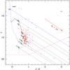 |
Fig. 10 J vs. J − H CM diagram for YSOs of the Sh2-90 complex. The PMS isochrones of 1 Myr from Siess et al. (2000) and Baraffe et al. (1998) are drawn in solid and dashed curved lines (black), respectively, for a distance of 2.0 kpc and zero reddening. The reddening vectors corresponding to 0.1, 0.15, 0.2, 0.5, 1, 3, and 4 M⊙ are drawn in dotted slanting lines. The ZAMS (vertical dashed line in blue), along with the reddening vector (slanted line in blue) from the tip of the B0 star, is also shown. The average error in color is shown on the upper-right side of the figure. |
In total, we have identified 129 sources in the Sh2-90 complex with excess IR emission. Of these, 21 have excess consistent with Class I YSOs, 34 have excess consistent with Class II or Class I/II YSOs, and 74 are termed as NIR-excess YSOs (i.e., sources not classified as YSOs based on IRAC colors). We did not classify diskless YSOs (Class III sources), because with the present data sets they are indistinguishable from field stars. We note that although the NIR and IRAC colors are very useful for identifying YSOs, the YSOs classification can be altered based on the high degree of reddening and viewing angle. Nevertheless, the assumed classification scheme provides a good representation of the respective YSO classes. The catalog of the identified YSOs in the present analysis is given in Table 5. A sample of Table 5 is given here; the complete table is available in electronic form at the CDS.
6.2. Mass distribution of the YSOs
Having identified YSOs, we can quantitatively constrain their stellar masses with an assumed age. Since YSOs generally show excess emission at long wavelengths, to minimize the effect of excess emission on masses we use J vs. J − H colour–magnitude (CM) diagrams. Figure 10 represents the intrinsic J vs. J − H CM diagram for 109 sources (out of the 129 excess sources), having counterparts in J and H bands. To produce the intrinsic CM diagram, the extinction in front of YSOs is derived by tracing back their observed colors to the CTT locus or its extension in (J − H) vs. (H − K) CC diagram along the reddening vector. The solid and dashed curves in the figure denote the loci of 1 Myr PMS isochrones by Siess et al. (2000) for 1.2 M⊙ ≤ M ≤ 7 M⊙ and Baraffe et al. (1998) for 0.05 M⊙ ≤ M ≤ 1.4 M⊙, respectively. The dotted slanting lines are the reddening vectors for 4, 3, 1, 0.5, 0.2, 0.15, and 0.1 M⊙ stars for 1 Myr isochrones. Figure 10 suggests that the ages of most of the YSOs are probably 1 Myr or less. Here, we would like to mention that age estimation of young clusters by comparing the observations with the theoretical isochrones is prone to several errors such as unknown extinction, excess emission due to disk, variability, and binarity; the ages can be therefore highly discrepant. Here, we do not intend to estimate the exact masses of the YSOs, rather we would like to know their approximate masses. Since the PMS isochrones for low-mass stars are very close to each other, a change in age of 0.5−1 Myr would not change drastically the masses of the low-mass YSOs. Thus, we considered 1 Myr as a representative age to estimate the mass of the YSOs. It is worth noting that adopting different sets of evolutionary tracks would provide different values of stellar masses. However, for low-mass objects, the tracks of Siess et al. (2000) are close to those of Baraffe et al. (1998). The agreement between ages and masses of these two models is within 20−40%.
The dotted (red) line indicates the approximate completeness limit of our NIR data. Figure 10 shows that for the assumed age of 1 Myr, the lowest YSO mass down to which our J-band image is largely complete is about 0.2 M⊙ for AV~ 8 mag (the mean AV of all the YSOs). From the figure it appears that most of the identified YSOs have masses in the range of 0.2−3 M⊙, except a few sources whose locations fall close to the reddened zero-age-main-sequence (ZAMS) star of spectral type B0.
6.3. The spatial distribution of YSOs
We identified 129 YSOs using IRAC and NIR colors. The spatial distribution of these YSOs on the column density map is shown in Fig. 11. The YSOs (Class 0/I in red, Class II in yellow, and NIR-excess in green) are found to be preferentially located in/around regions of high column density, with enhanced concentration at the locations of C1 and C5. We note that the location of C5 is close to the H ii region Sh2-90, whereas C1 is located far away from it. We discuss possible star formation processes at these locations in Sect. 8. The figure also displays that the majority of the Class 0/I YSOs are found to be distributed in the directions of f1, f2, f3, and clump C5, whereas the NIR-excess YSOs show a slightly scattered distribution, but in general the YSO distribution follows the elongated nature of original cloud seen in the CO map of Lafon et al. (1983) and in our 350 μm image (see Figs. 4 and 6). To verify whether the observed trend of the YSO distribution in the small filament-like structures (f1, f2, and f3) is due to the effect of extinction to the photometric colors or if they are really sources with emission from the disks and envelopes, we estimated the column density towards these structures and relate its effect on the photometric colors. The mean column density of f1, f2 and f3, is ~1.4 × 1022 cm-2, ~1.3 × 1022 cm-2, and ~8.9 × 1021 cm-2, respectively, although the column density in the direction of individual YSO can vary depending on their exact location. These values correspond to mean visual extinction ~15, 14, and 9.5 mag, respectively (using N(H2) = 0.94 × 10²¹AV cm-2 mag-1; Bohlin et al. 1978; Rieke & Lebofsky 1985). These extinction values are possibly underestimated owing to the low spatial resolution of our column density map. However, a visual extinction value of 20 mag can only produce a shift of 1.07, 0.26, 0.06, and 0.05 mag in K–[4.5], [3.6]−[4.5], [4.5]−[5.8], and [5.8]−[8.0] colors, respectively (based on extinction laws of Flaherty et al. 2007). Thus, we anticipate that the most of the identified YSOs are real YSOs of the complex. We note that the quoted extinction values are determined assuming that the extinction law of the general diffuse ISM (i.e., total-to-selective extinction = 3.1) is valid, which may not be the case for very dense regions. In such cases, the extinction values can be increased by a factor of 1.37, if RV reaches a value of 5.5 (see Weingartner & Draine 2001; Dunham et al. 2011).
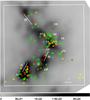 |
Fig. 11 Spatial distributions of Class I (red circles), Class II (yellow circles), and NIR-excess (green circles) YSOs on the column density map centerd at α2000 = 19h49m22s, δ2000 = + 26°50′15′′. The horizontal bar is labeled in units of cm-2. The box represents the area for which Class I, Class II, and NIR-excess YSOs have been searched. North is up and east is to the left. |
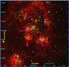 |
Fig. 12 Left: color-composite image of Sh-90 centered at α2000 = 19h49m13sδ2000 = + 26°49′54′′, showing point sources at 1.25 μm (blue), 2.14 μm (green), and 5.8 μm (red). The names refer to the different IR blobs (see Sect. 6.4) and 250 μm clumps (see Sect. 5.3) identified in the complex. The yellow contours represent the 250 μm clumps. The contours are at 1450, 2000, and 3000 MJy sr-1. The small circles mark the position of the NIR sources that lie within these IR blobs and clumps. North is up and east is to the left. |
6.4. Nature of sources within IR blobs and/or clumps
Polycyclic aromatic hydrocarbon emissions can be used as tracers of embedded B-type star formation (Peeters et al. 2004). These stars have the ability to heat the surrounding dust to high temperatures, and can excite the PAH bands and fine-structure lines. We see several compact dust emission features (e.g., IR1, IR2, IR3, and IR4) at 8 μm, 24 μm, and/or 70 μm (see discussion in Sect. 4.1 and Fig. 12), similar to those seen at the peripheries of the bubbles such as RCW 79 (Zavagno et al. 2006, their clumps 2 and 4) and RCW 120 (Zavagno et al. 2007, their clump 4). These compact IR structures are possibly a tracer of low luminosity (log (L/L⊙) = 1.5−4.4) embedded massive B-type stars. Hence, for discussion purposes, hereafter we collectively called these compact IR structures as IR blobs.
In order to identify the probable massive members in the IR blobs and in the clumps C1 to C9 (some of them are co-spatial with the IR blobs), we used our sensitive, high-resolution JHKs catalog. We visually searched for the counterparts of the bright IRAC and NIR sources, within the approximate boundary of these blobs or clumps. The probable sources are marked in Fig. 12, and the positions of these sources are also shown in the (J − H) vs. (H − K) (Fig. 13, right) and J vs. (J − H) (Fig. 13, left) diagrams. Many sources show NIR excess in Fig. 13 (right); therefore, the stellar luminosity of such sources in the J vs. (J − H) diagram is uncertain and should be considered as an upper limit.
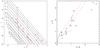 |
Fig. 13 Left: J vs. J − H diagram for luminous sources found within the IR blobs and clumps of the Sh2-90 complex. The ZAMS locus reddened by AV= 0, 10, 20, and 30 mag is shown in vertical dot-dashed lines. Slanting solid lines represent the standard reddening vector drawn from the ZAMS locus corresponding to different spectral types. Right: J − H vs. H − K diagram for the same sources. The thin solid (blue) and thick dashed (green) lines represent the unreddened MS and giant branches (Bessell & Brett 1988), respectively. The dotted line (blue) indicates the intrinsic locus of T-Tauri stars (Meyer et al. 1997). The parallel dashed lines are the reddening vectors drawn from the tip of the giant branch (left reddening line) and from the base of the MS branch (right reddening line). The sources with IDs represent the same sources as in Fig. 12, except source 21 because its colors (J − H = 5.6 mag, H − K = 3.6 mag) fall well beyond the range shown in the plot. |
Physical parameters of the YSOs derived from the SED fittings.
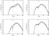 |
Fig. 14 The Robitaille et al. (2007) SED models of the four luminous embedded YSOs in the region (see text). The black line shows the best fit, and the gray lines show subsequent good fits that satisfy |
For four luminous embedded YSOs (IDs 10, 13, 21, and 25), for which we have well sampled fluxes from NIR to 350 μm, we fit models of Robitaille et al. (2007). These models are computed using Monte Carlo based radiation transfer codes using several combinations of central star, disk, in-falling envelope, and bipolar cavity for a reasonably large parameter space. The fluxes of these four luminous sources at Herschel bands have been taken from the Curvature Threshold Extractor package (CuTeX) catalog. The details about the catalog and the photometric procedures adopted in CuTeX are given in Molinari et al. (2011, and references therein). While fitting the SED models, we adopted 10% to 30% errors in the flux estimates and allowed distances in the range of 2.1−2.5 kpc. From SED models we constrained the key physical parameters such as stellar mass (M∗), stellar temperature (T∗), disk mass (Mdisk), disk accretion rate (Ṁdisk), visual extinction (AV), and the total luminosity (Lbol). The SED models of the four luminous sources are shown in Fig. 14 and their physical parameters are tabulated in Table 6. The tabulated values are the weighted mean and standard deviation of the parameters obtained from the best-fit models (i.e., models satisfying  , where
  is the goodness-of-fit parameter for the best-fit model and Ndata is the number of input observational data points) weighted by e(−χ2/2). The resolution of Herschel images is larger than the resolution of NIR and Spitzer images (see Sect. 3), thus the contribution from the surrounding environments to the flux estimates of these YSOs at Herschel bands (particularly λ ≥ 160 μm), cannot be ignored. If this is the case, among the model-based parameters, the parameter total luminosity is likely to be affected most and is probably an overestimation. Similarly, inclination angle can also vary the SED shapes, and so the parameters. Thus, because of several aforementioned limitations, the model-based parameters are only indicative of stellar and circumstellar properties of the underlying stellar source. Nevertheless, from Table 6 it can be inferred that for all the four sources the model based parameters seem to be constrained well, except source 21 for which the disk accretion rate is not well constrained. The limitations of the SED based models, while inferring physical parameters have been discussed in Robitaille (2008). For example, for embedded Class 0/I sources, the Robitaille et al. models omit dust temperatures below 30 K, whereas the average envelope temperature of Class 0/I YSOs are generally lower (e.g., ~ 15.7 ± 1.7 K in the W5 complex; Deharveng et al. 2012). In such cases, the models overestimate the envelope mass (Menv) of a YSO to account for fluxes at longer wavelengths. The four luminous YSOs have been detected in the NIR and MIR bands, thus protostars have formed. The disk is a significant contributor to the SED shape at λ ≤ 100 μm (Whitney et al. 2005). We are mostly interested in the envelope mass. We thus computed the Menv of the luminous YSOs by fitting a modified blackbody to the observed fluxes at 160, 250, 350, and 500 μm in order to avoid the contribution of warm dust at 70 μm (due to internal heating from the protostar and emission from the disk). The modified blackbody fits of the four luminous YSOs are shown in Fig. 15 and the derived Menv values are tabulated in Table 6.
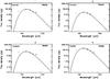 |
Fig. 15 Graybody SEDs of the envelopes of the four luminous embedded YSOs in the region. The black line shows the best modified blackbody fit to the data points, between 160 μm and 500 μm. The circles denote the input flux values. |
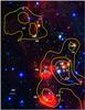 |
Fig. 16 Color-composite image of the regions IR1, IR2, IR3, C5, and C6 at 5.8 μm (red), 2.14 μm (green), and 0.80 μm (blue), with 250 μm contours. The contour levels are at 1450, 2000, and 3000 MJy sr-1. North is up and east is to the left. |
In the following, we discuss the nature of the luminous sources within the clumps and IR blobs.
Clump C7: this is a 250 μm clump of mass ~95 (89) M⊙. In the western direction of the clump a 24 μm roughly circular (diameter ~24 ) diffuse dust emission (see Fig. 2) is observed. The YSOs found in the direction of C7 are distributed along the ionization front (PDR seen in 8 μm and 70 μm) of Sh2-90. The luminous IR objects in the proximity of C7 are marked (labeled 7 and 14) in Figs. 12 and 16. Source 7 is luminous in all IRAC bands. Its position in the J vs. J − H diagram indicates an early B star, reddened by AV~ 16 mag. This source shows weak IR excess in the J − H vs. H − K diagram and no compact radio emission is detected in its direction, thus the possibility that it appears luminous because of excess emission at the J and H bands exists. Hence the present luminosity (mass) of the source is possibly an upper limit. For a PMS star of an assumed age of 1 Myr (see Sect. 6.1), its location on the HR diagram suggests that it is a source of mass greater than 4 M⊙. Future spectroscopic observation would reveal the exact nature of the source. The position of source 14 in Fig. 13 suggest that it is probably an intermediate-mass (B8-type) YSO with extinction ~18 mag. Clump C7 consists of two sub-clumps. The two sub-clumps probably follow two PDRs seen in the 8 μm and 70 μm map.
Region IR2: the region displays a circular (diameter ~22) diffuse dust emission in the wavelength range 5.8−70 μm. The luminous sources found within IR2 are marked (labeled as 1, 4, and 12) in Figs. 12 and 16. None of them shows sign of NIR excess. Two sources, sources 1 and 4, appear to be reddened background objects, as their position on J − H vs. H − K diagram falls close to the reddened giant locus. The position of source 12 on the J vs. J − H diagram (Fig. 13) indicates a star of B7-type, reddened by AV~ 10 mag. This source is the most-likely star responsible for the excitation of the 5.8−70 μm dust in IR2. This region is devoid of cold dust emission at λ ≥ 160 μm.
Region IR3: the morphology of IR3 is similar (diameter ~20) to IR2 in the range 5.8−70 μm. In NIR, we detect a bright point source (labeled as 3 in Figs. 12 and 16) at the center of IR3. The position of this source on NIR diagrams (Fig. 13) indicates a star of spectral type close to B3, extincted by AV~ 13 mag with no NIR excess. Being situated at the center of the nebula, it is the most-likely heating source of IR3. A 250 μm clump (C4) of mass 26(20) M⊙ lies adjacent to IR3.
Clump C5: this is a 250 μm clump of mass ~125 (75) M⊙. In NIR, we identified four bright sources (labeled as 2, 6, 9, and 10 in Figs. 12 and 16) close to the peak of C5, among which two sources (2 and 10) show strong IR excess and appear luminous in J vs. J − H diagram, with spectral type earlier than B2 and extinction greater than 27 mag (if purely photospheric). Since both the sources show strong NIR excess, their stellar luminosity based on J vs. J − H is not reliable. Both the sources are of Class 0/I in nature; however, the emission at Herschel wavelengths, is mainly dominated by source 10. The parameters (ID 10 in Table 6) obtained from the best-fit Robitaille et al. (2007) models (top left in Fig. 14) suggest it is a ~6 M⊙ star of total luminosity of ~ 0.7 × 10³ L⊙ embedded in a cloud of AV~ 16 mag. We also fit the SED models to source 2 with input fluxes in the range 1.25−22.0 μm to constrain some of its basic parameters. The 22 μm flux has been adopted from WISE survey (Cutri et al. 2014). The models suggest it is a ~5 M⊙ star of total luminosity ~ 0.9 × 10² L⊙ embedded in a cloud of AV~ 18 mag. Source 6 is optically bright, highly luminous in J vs. J − H diagram with no excess, and is located close to the unreddened giant locus in the J − H vs. H − K diagram, thus likely to be a foreground field star.
Towards C5, dense molecular tracers such as CS (Beuther et al. 2002) and NH3 (Wu et al. 2006) have been observed. The signature of high-velocity CO gas (Yang et al. 2002) has also been reported towards C5. We identified a significant number of YSOs in the close proximity of C5 (see Fig. 11), thus possibly suggesting a cluster forming site.
Clump C6: this is a 250 μm clump of mass ~31 (17) M⊙ located towards the projected center of the N133 bubble. The luminous IRAC source associated with C6 (labeled as 13 in Figs. 12 and 16) is a Class 0/I YSO. Its position on NIR diagrams (Fig. 13), indicates a star of spectral type earlier than B1, extincted by AV> 32 mag (if purely photospheric). This source shows strong NIR excess, thus its nature is uncertain. The parameters (ID 13 in Table 6) obtained from the best-fit Robitaille et al. (2007) models (top right of Fig. 14) suggest it is a ~7 M⊙ star with total luminosity of ~ 0.8 × 10³ L⊙, embedded in a cloud of AV~ 12 mag.
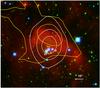 |
Fig. 17 Color-composite image of the region IR4 at 5.8 μm (red), 2.14 μm (green), and 0.80 μm (blue), overlaid with 250 μm contours (yellow). The contour levels are at 1450 MJy sr-1 and 2000 MJy sr-1. The white contours represent the radio continuum emission at 1280 MHz. North is up and east is to the left. |
Region IR4: the region shows a cometary structure at 8.0 μm, partly protruding into the H ii region. The location of IR4 coincides with IRAS 19471+2641 of luminosity ~ 7.7 × 10³ L⊙. In our high-resolution radio continuum map, we identified a compact radio source (shown in Fig. 17) of flux density ~0.04 mJy, which corresponds to ionizing photon flux from a star of spectral type B1 V (Smith et al. 2002). Three bright point sources (labeled as 17, 18, and 23 in Figs. 12 and 17) are found inside it. Among these sources, source 23 is the most luminous source in NIR, and its location on NIR diagrams (Fig. 13) suggests that it is a source of spectral type B2–B3, reddened by AV~ 7 mag. The other two sources also appear as B-type (B5–B7) stars. This compact H ii region is most probably ionized by source 23. The hot dust appears as circular and extended at 24 μm and 70 μm around these B-type stars. A PDR is seen around these sources at 8.0 μm or 5.8 μm. We identified a 250 μm clump (C3) of mass ~37 (28) M⊙ adjacent to IR4. The PDR is bright in the direction of C3.
Clump C9: this is a 250 μm clump of mass ~19 (16) M⊙ located on the PDR of Sh2-90. This region coincides with the position of IRAS 19470+2643 of luminosity ~ 7.6 × 10³L⊙. The luminous sources near C9 are marked in Fig. 12 (labeled as 5, 11, and 24). Source 11 appears to be a B5 in the J vs. J − H diagram; however, its location is close to the unreddened giant locus in the J − H vs. H − K diagram, thus it is probably a foreground field star. The position of the sources 5 and 24 on the J vs. J − H diagram (Fig. 13) shows the characteristics of a spectral type earlier than B3, with AV> 19 mag. These sources do not show NIR excess, and the maximum column density in the direction of C9 suggests an extinction of ~9 mag. These sources are slightly relatively more reddened than the other massive sources associated with the regions such as IR1, IR2, IR4, and IR4 observed in the PDR of Sh2-90. No 8 μm or 24 μm symmetric emission structures have been noticed around C9. Thus, we suspect that the bright NIR sources of C9 are probably reddened background objects, which is also supported by the location of 24 on the J − H vs. H − K diagram.
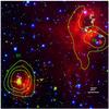 |
Fig. 18 Color-composite image of the regions N132 and C1 at 5.8 μm (red), 2.14 μm (green), and 0.80 μm (blue), overlaid with 250 μm contours. North is up and east is to the left. |
Region N132/C2: N132 is roughly a circular bubble of diameter ~028, with a central cavity and a thin annular shell bordering it. The shell is best seen at 8.0 μm. Unlike N133, it is not visible in the optical. No 23 cm emission has been observed towards N132, thus this infrared dust bubble was possibly created by a less massive star than the O-B2 stars. The luminous sources (labeled as 15, 19, and 20) projected inside the bubble are marked in Figs. 12 and 18. The position of source 19 on the J vs. J − H diagram suggests it is a star of spectral type close to B3, extincted by ~9 mag, whereas the location of other sources (15 and 20 in Fig. 18) possibly suggests that they are cooler stars; because these stars possess IR excess, they appear luminous in the J vs. J − H diagram. A clump (C2) of mass ~43 (37) M⊙ lies close to the southwestern boundary of N132 (see Fig. 18). A source (ID 25) at the center of this clump is visible in all the IRAC bands, and its IRAC colors are consistent with a Class 0/I YSO. This source is not detected in J and H bands, thus is highly embedded. The parameters (ID 25 in Table 6) from the best-fit SED models (bottom left in Fig. 14) suggest it is a ~6 M⊙ star with a total luminosity ~ 0.6 × 10³ L⊙ embedded in a cloud of AV~ 42 mag.
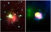 |
Fig. 19 Left: Color-composite image of the region C1 at 5.8 μm (red), 4.5 μm (green), and 3.6 μm (blue). Right: Color-composite image of the same region at 70 μm (red), 24 μm (green), and 8.0 μm (blue). North is up and east is to the left. |
Clump C1: this is a clump of mass 206 (186) M⊙. The clump is bright at Herschel bands. It is associated with a point source (ID 21 in Fig. 18) seen in all wavelengths between 1.25 μm and 500 μm. At longer wavelengths (≥250 μm) elongated extended emission (i.e., in the direction of f1; see Fig. 3) is seen in the N-W direction of C1. A faint diffuse 24 μm emission can also be seen in its N-E direction (see Fig. 19). This source shows strongest IR excess in the J − H vs. H − K (i.e., J − H = 5.6 and H − K = 3.6) CC plot and is the most luminous one in the J vs. J − H diagram (it does not appear in Fig. 13). Its IRAC colors suggest that it is a Class 0/I YSO. The parameters (ID 21 in Table 6) obtained from the best-fit Robitaille et al. (2007) models (bottom right in Fig. 14) suggest it is a ~8.8 M⊙ star with a total luminosity of ~ 4.0 × 10³ L⊙ embedded in a cloud of AV~ 31 mag.
The location of C1 coincides with IRAS 19747+2637 of luminosity ~ 1.4 × 10⁴ L⊙. No 1.3 cm continuum emission is detected towards IRAS 19747+2637 at rms of 0.7 mJy beam-1 (Wang et al. 2007). The 0.7 mJy flux corresponds to the number of Lyc photons of ~ 2.1 × 1044 s-1 (spectral type later than B2 V). Therefore, the present upper limit on mass of the massive source expected to be ~10 M⊙. The source IRAS 19747+2637 is associated with a H2O maser (Codella & Felli 1995). Observation in the CO line (J = 1 − 0, Xu et al. 2001; Yang et al. 2002) suggested that IRAS 19747+2637 is associated with a high-velocity gas, thus is an outflow candidate; SiO emission has been detected in this region, which increases the possibility of shocks associated with massive young sources (Harju et al. 1998). The detection of a maser and signature of shock suggest that the luminous YSO is at its early evolutionary phase. The cloud containing this luminous YSO also harbors many low-mass YSOs (with masses ≤3 M⊙). The detection of a large number of YSO candidates in the close vicinity of C1 suggests a site of cluster mode of massive star formation, where the massive star has not yet developed an ultra compact H ii region. This is probably a site of young cluster in the process of formation.
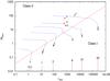 |
Fig. 20 Lbol vs. Menv diagram for the massive YSOs (solid circles with IDs). The dotted blue lines represent the evolutionary tracks from André et al. (2008). Evolution proceeds from the upper left to the lower right (indicated by arrows at the end of each track). The final stellar masses of these tracks in solar units are given above the lower axis. The slanted red line corresponds to the location where 50% of the initial core mass is converted into stellar mass (see Bontemps et al. 1996; André et al. 2000). |
6.5. Evolutionary status of massive sources
The SED models suggest that the IR sources (IDs 10, 13, 21, and 25) are massive (6−9 M⊙) and of high luminosity (0.4 − 4 × 10³ L⊙). These sources are classified as Class 0/I YSOs based on IRAC data; however, there is scope to revise further the classification of individual Class 0/I YSOs in the light of Herschel observations. For these sources, we found high values of submillimeter to bolometric luminosity (Lλ ≥ 350 μm/Lbol> 0.2 M⊙/L⊙), envelope mass to the mass of central protostar (Menv/M⋆> 3.4), and envelope mass to bolometric luminosity (Menv/Lbol> 0.03), indicating they are more likely to be Class 0 protostars (see André et al. 2000) in their accretion phase. We also use the physical parameters obtained for the sources to infer their evolutionary status using Menv–Lbol diagrams (André et al. 2000; Molinari et al. 2008). The location of these four sources on the Menv–Lbol evolutionary diagram for protostars is shown in Fig. 20, and their comparison with the evolutionary tracks of (André et al. 2008, and references therein), suggests that these objects will evolve into stars of mass ≥15 M⊙. In summary, these YSOs are massive YSOs (MYSOs) of the region likely to be in their Class 0 or early Class I stage. It is especially evident for 10 and 21, as signatures of outflow (e.g., high velocity CO gas or SiO emission) and/or maser emission have been observed in both cases (Harju et al. 1998; Xu et al. 2001; Yang et al. 2002).
Are these four MYSOs in different evolutionary stages than the massive sources associated with the IR blobs (IR1, IR2, IR3, and IR4)? In the absence of the stellar properties (e.g., stellar luminosity and temperature) and the lack of sensitive longer wavelength observations to model the SEDs of the massive sources in the IR blobs, a clear distinction cannot be made. However, from the available physical conditions of their environment and stellar properties, the evolutionary status of these two groups can be inferred up to a certain extent. It is expected that the mass of the cold components decreases with time as the protostellar envelope accretes onto the central object and progressively the central massive protostar emerges from the cloud by dispersing its natal environment. Although the four MYSOs are visible in NIR, they show strong NIR excess and a large fraction of their luminosity lies in the far-infrared to submillimeter regime (see Fig. 14). They are surrounded by cold components and thus possibly actively accumulating material from the cold envelope. The massive source(s) of IR blobs are optically visible, show little or no IR excess, and cold components are often not found at their exact locations, all of which indicates that they have little or no circumstellar dust left. The above characteristics strongly suggest that the massive sources of the IR blobs should represent an older evolutionary sequence than the envelope-dominated likely Class 0/I MYSOs of the complex.
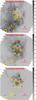 |
Fig. 21 The 12CO(J = 3 − 2) integrated emission in the direction of Sh2-90 centered at α2000 = 19h49m14s, δ2000 = + 26°50′01′′. Velocity ranges are indicated at the top of each image. The horizontal color bars are labeled in units of K km s-1. The data is from Beaumont & Williams (2010). The overlaid 250 μm contours are at 1450, 2000, and 3000 MJy sr-1. The clumps discussed are marked (see also Fig. 12). North is up and east is to the left. |
7. Kinematics of ionized and molecular material, and evolutionary status of Sh2-90
We used the 12CO (J = 3 − 2) data cubes of Beaumont & Williams (2010) to study the association of the cold dust clumps discussed in Sect. 5.3. The inspection of data cubes showed that the CO emission over the whole field is mainly in the velocity range 15.5−28.5 km s-1(only weak CO emission is seen outside this velocity range). We isolate the CO emission of the Sh2-90 complex along the line of sight mainly into three major components: i) 16.1−20.1 km s-1; ii) 20.1−24.1 km s-1; and iii) 24.1−28.1 km s-1. Figure 21 shows the distribution of integrated CO emission as a function of velocity in these velocity ranges:
-
The 16.1−20.1 km s-1component shows a cavity corresponding to the location of Sh2-90 and an extended diffuse cloud at the east and south of Sh2-90. We also observed similar extended dust emission towards the east and south of Sh2-90 in our column density map (see Fig. 7). This velocity component also displays prominent emission at the location of N132 (or C2) and IRAS 19474+2637 (or C1), thus confirming the association of these clumps with the complex.
-
Gas in the interval from 20.1 km s-1−24.1 km s-1shows enhanced molecular emission in a ring-like structure that resembles the Herschel 250 μm dust shell observed at the periphery of Sh2-90 (see Fig. 8). This possibly represents the collected matter around the H ii region. The clumps C3, C4, C7, C8, and C9 are projected on this ring-like CO emission, thus they are likely to be associated with Sh2-90. The feature south of C5 is more prominent in the velocity interval from 21.1 km s-1to 22.7 km s-1and for more positive velocities its peak emission shifts towards C5.
-
In the 24.1 to 28.1 km s-1range, the features of C7 and C9 remain visible; however, the strongest molecular emission at these velocities is mainly coincident with region C5.
-
Clump C6 is projected towards the center of Sh2-90; its association is difficult to determine because we did not notice any strong CO emission at the exact location of C6.
Lafon et al. (1983) observed ionized gas emission towards Sh2-90, using the optical Hα line, in the velocity range VLSR~ 8–33 km s-1with a mean velocity of 20.8 km s-1. Although their velocity map shows complex velocity distribution, which could be due to the effect of strong irregular extinction across the region, the velocity distribution mainly shows VLSR≥ 26 km s-1in the N-W side (corresponding to the brightest zone of optical emission) and VLSR≤ 14 km s-1in the S-E side of Sh2-90. This velocity range is consistent with the velocity range of the molecular gas discussed above. The large velocity range covered by the ionized gas may be indicative of a “champagne flow” (Tenorio-Tagle 1979). Although in our low-resolution 610 MHz radio map, we see a weak gradient in brightness distribution from N-W to S-E direction, on a large scale the shape of ionized gas appears to be more symmetrical (see Fig. 3) with ionizing star(s) at the center of nebula. Thus the H ii region is possibly in its early phase of “champagne-flow”.
During the evolution of the H ii region, if the ionized gas expands spherically, then the difference in the extreme radial velocities (either blueshifted or redshifted) should roughly reflect its expansion velocity. If we consider the velocity measurements at the two projected opposite edges of Sh2-90 (i.e., 26 km s-1N-W and 14 km s-1S-E) as the extreme radial velocity values of the H ii region, then this would indicate a crude expansion velocity of ~6 km s-1.
Here, we tried to derive the dynamical age of the H ii region, based on the observed properties and assuming that the H ii region evolved in a homogeneous medium. The ionizing photon flux coming from the massive stars associated with Sh2-90 is ~ 22.5 × 1047 s-1. The radius of the H ii region is ~1.6 pc. The density of the original medium is unobservable; only an approximate value can be adopted based on the present observable indicators. The average density of clumps in the shell is ~7(5) × 103 cm-3 (see Table 4), which possibly represents an upper limit (assuming it has purely formed from the collected matter). A lower limit on density of the original medium estimated from the total ionized gas of the H ii region and neutral matter collected in the shell is ~2.6 (2.0) × 103 cm-3 (see Sect. 5.3). Considering that the H ii region is expanding at velocity ~6 km s-1, in a homogeneous medium of density in the range 2 − 7 × 103 cm-3, and following the model by Dyson & Williams (1997), we estimated the dynamical age (i.e., the time it would take to form from its initial Strömgren sphere to its present size) in the range 0.6 − 1.2 × 10⁶ yr. We caution that this age estimations should not be taken too literally, because of the possible existence of a “champagne-flow" and the assumption of evolution in a homogeneous medium, which is probably far from the truth. The MS lifetime of an O8 star is on the order of ~ 6.5 × 10⁶ yr. This allows us to constrain the dynamical age younger than 6.5 × 10⁶ yr.
8. Star formation scenarios in the complex
Based on multi-wavelength observations presented in this work our understanding of star formation associated with the Sh2-90 complex can be summarized as follows:
-
The Sh2-90 H ii region was createdby an O8–O9 star (see Sect. 4.4).The O-type star possibly formed 1 Myr ago (seeSect. 7), created ionized gas around itself whichthen expanded, sweeping ambient ISM gas and dust into a bubble.The morphological correlation between ionized gas, PDR, andring-like dust emission (see Sects. 4.2and 5.3) around the ionized gas led us to believethat there is certainly a high degree of interaction between theUV photons from the massive star and thesurrounding molecular cloud.
-
Herschel cold dust properties and Spitzer point source analyses reveal that star formation in the complex is not confined to the Sh2-90 H ii region (see Sects. 5.3 and 6.3). Several sites of star formation have been observed in this massive (M > 104 M⊙) cloud. The main star-forming sites are associated with the complex as they have similar velocities (see Sect. 8.5). Based on the velocities of the molecular and ionized gas, and signs of interaction of the Sh2-90 bubble with the molecular gas, we believe that most of the extended cold dust emission seen at Herschel wavelengths is associated with the complex.
-
The column density map presents an elongated structure similar to that seen on the low-resolution (4.́4) 13CO map (Lafon et al. 1983). We identified 129 likely YSO candidates, which includes 21 Class I, 34 Class II, and 74 NIR-excess YSOs. (see Sect. 6.1). The spatial distribution of YSOs follows the distribution of the high column density matter (see Sect. 6.3). As these young sources have not had time to move away very far from their birthplaces, this indicates that the elongation and sub-clustering of young sources possibly resulted from the primordial distribution of the parental dense gas in this complex.
-
We identified four Class 0/I MYSOs in their main accretion phase (see Sect. 6.5). The simultaneous presence of envelope-dominated Class 0/I MYSOs at various locations and of the ionizing star of an evolved H ii region (age ~ 1 Myr; see Sect. 7) in the same complex suggests that different episodes of star formation have occurred in this complex. How star formation occurred at different locations in this extended cloud is difficult to determine. Large-scale SFRs often contain smaller size cores/clumps of high column densities possibly due to density fluctuations present in the original cloud. Star formation can occur in these cores/clumps on a local dynamical time scale as long as the local conditions are close to gravitationally bound and so can result in multiple stellar groups in the same complex, possibly in different evolutionary stages. However, since Sh2-90 is an evolved H ii region, we can also speculate that the formation of young sources in the region might have been triggered by the expanding bubble. We will discuss this aspect in the following. However, smoothed particle hydrodynamic simulations (Dale & Bonnell 2011; Dale et al. 2012) have shown that several untriggered stars can be formed in the extended environment of bubbles/H ii regions by other processes, including spontaneous ones.
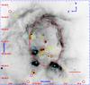
Fig. 22 Morphology of the region at 8.0 μm, overplotted with Class 0/I (red circles) and Class II (yellow circles) YSOs. The position of the B-type sources are marked with plus signs. The ellipse represents the projected boundary of the 8.0 μm cavity.
Similar to the findings of Deharveng et al. (2010), Thompson et al. (2012, based on the Red MSX Source survey of MYSOs) suggested that the formation of only about 14% to 30% of the massive stars in our Milky Way could have been triggered or influenced by H ii regions, whereas the remaining 86% to 70% stars are likely to be formed by other processes. Although most of the identified YSOs in the Sh2-90 complex are of low mass (<3 M⊙; see Sect. 6.2), 67% of them are situated beyond the bubble projected radius. The Sh2-90 complex is extended and clumpy (see Fig. 7, bottom), thus some of the YSOs could be the result of spontaneous star formation. In particular, if we considered SFRs such as IRAS 19474+2637 (or C1) and IRAS 19473+2638 (or C2), then their locations beyond the main interaction zone of the bubble suggest that the star formation in these regions is unlikely to be triggered by the expansion of Sh2-90. We calculated that the ionizing photon flux from the ionizing star at the location of IRAS 19474+2637 (~4.7 pc away) and IRAS 19473+2638 (~3.2 pc away) is less than 109 cm-2 s-1, the flux required to trigger star formation even in a low-mass (<5 M⊙) cloud (Bisbas et al. 2009). From the above evidence, we hypothesize that some of the YSOs (particularly the distant regions forming MYSOs) in the complex, could have formed spontaneously or by some other processes.
-
The star formation activity at the periphery of Sh2-90 is somewhat different. We observed that young B-type stars associated with 8−24 μm compact circular structures such as IR2, IR3, and IR4 lie at the edge of Sh2-90. Our search in a wider area with IRAC and MIPS images, resulted in no such compact, spatially closed circular structures, thus their chance of alignment along the line of sight is unlikely. They are possibly young (supported by the compact nature of their radio and/or 8−24 μm dust emissions), although this cannot be warranted without spectroscopic observations. There are also seven distinct clumps C3, C4, C5, C6, C7, and C9 (the clumps C3, C4, and C7 are located adjacent to IR4, IR3, and IR1, respectively). The clumps C3, C4, C7, and C9 are part of the connecting shell of cold material which partially borders the 8 μm cavity. The distribution of B-type stars associated with IR structures and/or cold clumps around the periphery of Sh2-90 (age ~ 1 Myr), thus suggests that star formation has been possibly triggered in such regions. The case of C5 and C6 with MYSOs is not so clear. These clumps are seen in the direction of the ionized gas; they probably lie in front of it, as they are seen in absorption at optical bands. Thus the formation of the YSOs they contain can also be triggered. However, the velocity of C5 is more positive with respect to the mean velocity of the Sh2-90, and the evolutionary status of the clump C5 is similar to C1 and distinctly different from the sources within the IR blobs (see Sect. 6.4 and 6.5). Thus, the possibility that this could also be one clump like C1 located outside the action zone of Sh2-90 and going through star formation by some other processes cannot be excluded.
Proving the nature of triggered star formation around bubbles/ H ii regions formed in a non-uniform extended cloud is difficult, as triggered sources can be mixed with the spontaneously forming ones. The complex environment of Sh2-90 is a subject of concern, nonetheless, on a large scale the distribution of neutral matter in a shell-like structure, with massive clumps at regular intervals at its edges, suggests that the triggering might have happened through the collect and collapse (Elmegreen & Lada 1977; Deharveng et al. 2005; Zavagno et al. 2006) process of star formation, in which fragmentation occurs due to large-scale gravitational instabilities of the material accumulated during the expansion of the H ii region. We explore the feasibility of the collect and collapse process by comparing the observed properties with the predictions of the analytical models by Whitworth et al. (1994).
To compare, we adopt NLyc ~ 22.5 × 1047 s-1 from radio continuum observations and ~2(7) × 103 cm-3 as the density of the original medium (see Sect. 7) inside which the H ii region evolves. We consider the sound speed in the collected layer as ~0.3 km s-1, corresponding to an average temperature of the cold dust observed in the shell (see Sect. 5.2). With these values, the model predicts the fragmentation of the collected material after ~1.6(1.0) Myr at a radius of ~4.0 (2.0) pc, with fragments separated by some ~1.3(0.8) pc and having mass ≃84(47) M⊙. These predicted values are comparable with the observed properties, such as the dynamical age (~1 Myr) of the H ii region, the separation (~0.9 pc) between the B-type stars and the bound fragments, and the mass of the bound fragments (~17−125 M⊙) at the periphery of the bubble. However, the projected radius (~1.3 pc) at which B-type stars have been observed is smaller than the minimum radius ~2.0 pc predicted by the model. The above comparisons were done by simplifying facts throughout, as the caveats such as champagne flow, non-homogeneous medium, and projection effects always play crucial roles in such comparisons, and taking the present observational evidence at face value, the possibility of the young sources observed at the periphery of Sh2-90 might have formed through the collect and collapse process exists.
Alternatively, the Sh2-90 complex could be a case of star formation as found in the simulations of Dale et al. (2012) for bound turbulent clouds under the influence of internal ionizing sources. In their simulations Dale et al. (2012) infer objects which are triggered in a cloud complex by comparing the cloud with feedback sources with a control cloud without feedback sources. In all their simulations the triggered stars are found to be embedded in dense gas on the borders of feedback driven bubbles, and at the tips of pillars; but they are found to be mixed with the spontaneously formed ones. In the Sh2-90 complex B-type stars are formed at the periphery of the H ii region (see Fig. 22), but many low-mass (≤3 M⊙) sources of similar evolutionary nature are found to be formed far away as well as in the close vicinity of the H ii region (see Sect. 6.3). As discussed above, star formation seen at far away locations could be spontaneous (particularly at the location of C1). Thus, it is difficult to demonstrate that the formation of a specific source close to the H ii region is triggered by the H ii region rather than spontaneously; the geometrical distribution of some of the YSOs and young B-type stars close to the rim of the bubble (see Fig. 22) and their association with the cold gas (see Sects. 6.4 and 7); however, suggest that their formation is possibly triggered by the H ii region.
To put the star formation scenario of the complex on a firm footing, detailed velocity and age measurements of the sources in the complex are needed.
9. Conclusions
In this paper we have presented Herschel and radio continuum imaging of the Sh2-90 complex, as well as Spitzer-IRAC and deep NIR imaging to explore its stellar and interstellar content, and star formation history. Based on these observations our results can be summarized as follows:
-
1.
The Sh2-90 complex consists of two bubbles (N133and N132) and a few IRAS sourcesat various locations. N133 is a large bubble outlined by Spitzer8.0 μm emission and, together with Sh2-90, encloses the main H ii region of the complex. It is an evolved H ii region of diameter ~3.2 pc with an rms electron density ~144 cm-3, and an ionized mass ~55 M⊙. Our NIR photometry of the sources inside the bubble reveals the presence of a loose cluster, the most massive member of which is a O8–O9 V star that is responsible for the ionization of N133.
-
2.
The column density and temperature maps constructed from the Herschel observations suggest that Sh2-90 is part of a massive (≥104 M⊙) elongated cloud of column density ≥ 3 × 1021 cm-2. We observed that neutral collected material of mass ≥637 M⊙ is present in a shell surrounding the H ii region. Nine clumps are detected in the complex, among which seven (mass range 8−125 M⊙) are located at the periphery or in the direction of Sh2-90. Four of them are co-spatial with B-type stars and a compact H ii region. The velocity information of the clumps derived from CO (J = 3 − 2) data cubes suggests that most of them are likely to be associated with the Sh2-90 complex.
-
3.
Using the IRAC and NIR CC diagrams, we identified 129 likely YSO candidates of masses in the range of 0.2−3 M⊙, which includes 21 Class I, 34 Class II, and 74 NIR-excess YSOs. The photometric measurements of these YSOs are available in electronic form at the CDS. We identified four Class 0/I MYSO in their main accretion phase. We observed that the spatial distribution of the candidate YSOs follows the distribution of the high column density matter, with YSOs clustering at various locations, indicating that recent star formation is going on at multiple sites.
-
4.
We find the possible existence of two generation of massive to intermediate-mass star formation in the complex. One is in the immediate vicinity of the Sh2-90 H ii region, in the form of NIR/optical point sources responsible for the excitation of compact IR blobs and a compact H ii region, and the other in the form of young (~105 yr) Class0/I MYSOs.
-
5.
From the evolved state of the Sh2-90 H ii region, together with the presence of B-type stars and YSOs embedded in a thin shell of dense gas close to the IF of the H ii region, we suggest that the formation of these sources have possibly been triggered by the expansion of the H ii region. However, detailed velocity and age measurements of the stars in the H ii region could give more insights into this scenario.
In summary, it appears that multi-generation star formation is going on, but it remains unclear how the star formation sites and processes are interlinked. Taking the present observational evidence at face value, we suggest that triggered star formation possibly takes place at the immediate periphery of Sh2-90. However, we hypothesize that the MYSOs currently observed at various locations of the complex could have formed spontaneously or by some other processes.
The control region data were obtained from the GLIMPSE archive (Benjamin et al. 2003) and UKIDSS Galactic Plane Survey (GPS; Lawrence et al. 2007) at NIR bands.
Acknowledgments
We thank the anonymous referee for a critical reading of the paper and several useful comments and suggestions, which greatly improved the scientific content of the paper. M. R. Samal acknowledges the financial support provided by the French Space Agency (CNES) for his postdoctoral fellowship. We thank C. Beaumont and J. Dale for allowing us to use their CO observations and star formation simulation maps, respectively. This research has made use of the SIMBAD database operated at the CDS, Strasbourg, France, and of the interactive sky atlas Aladin. We acknowledge the support of data analysis facilities provided by the Starlink Project which is run by CCLRC on behalf of PPARC. This work used the observations obtained with the Herschel-PACS and Herschel-SPIRE photometers. PACS has been developed by a consortium of institutes led by MPE (Germany) and including UVIE (Austria); KU Leuven, CSL, IMEC (Belgium); CEA, LAM (France); MPIA (Germany); INAF-IFSI/OAA/OAP/OAT, LENS, SISSA (Italy); IAC (Spain). This development has been supported by the funding agencies BMVIT (Austria), ESA-PRODEX (Belgium), CEA/CNES (France), DLR (Germany), ASI/INAF (Italy), and CICYT/MCYT (Spain). SPIRE has been developed by a consortium of institutes led by Cardiff Univ. (UK) and including Univ. Lethbridge (Canada); NAOC (China); CEA, LAM (France); IFSI, Univ. Padua (Italy); IAC (Spain); Stockholm Observatory (Sweden); Imperial College London, RAL, UCL-MSSL, UKATC, Univ. Sussex (UK); Caltech, JPL, NHSC, Univ. Colorado (USA). This development has been supported by national funding agencies: CSA (Canada); NAOC (China); CEA, CNES, CNRS (France); ASI (Italy); MCINN (Spain); SNSB (Sweden); STFC and UKSA (UK); and NASA (USA). We thank the French Space Agency (CNES) for financial support. This work is based in part on observations made with the Spitzer Space Telescope, which is operated by the Jet Propulsion Laboratory, California Institute of Technology, under contract with NASA. We have made use of the NASA/IPAC Infrared Science Archive to obtain data products from the 2MASS, WISE, Spitzer-GLIMPSE, and Spitzer-MIPSGAL surveys.
References
- Allen, L. E., Calvet, N., D’Alessio, P., et al. 2004, ApJS, 154, 363 [NASA ADS] [CrossRef] [Google Scholar]
- Anderson, L. D., Zavagno, A., Deharveng, L., et al. 2012, A&A, 542, A10 [NASA ADS] [CrossRef] [EDP Sciences] [Google Scholar]
- André, P., Ward-Thompson, D., & Barsony, M. 2000, Protostars and Planets IV (Tucson: University of Arizona Press), 59 [Google Scholar]
- André, P., Minier, V., Gallais, P., et al. 2008, A&A, 490, L27 [NASA ADS] [CrossRef] [EDP Sciences] [Google Scholar]
- Arzoumanian, D., André, P., Didelon, P., et al. 2011, A&A, 529, L6 [Google Scholar]
- Baraffe, I., Chabrier, G., Allard, F., & Hauschildt, P. H. 1998, A&A, 337, 403 [NASA ADS] [Google Scholar]
- Beaumont, C. N., & Williams, J. P. 2010, ApJ, 709, 791 [NASA ADS] [CrossRef] [Google Scholar]
- Benjamin, R. A., Churchwell, E., Babler, B. L., et al. 2003, PASP, 115, 953 [NASA ADS] [CrossRef] [Google Scholar]
- Bergin, E. A., & Tafalla, M. 2007, ARA&A, 45, 339 [NASA ADS] [CrossRef] [Google Scholar]
- Bertin, E., & Arnouts, S. 1996, A&AS, 117, 393 [NASA ADS] [CrossRef] [EDP Sciences] [Google Scholar]
- Bertoldi, F., & McKee, C. F. 1990, ApJ, 354, 529 [NASA ADS] [CrossRef] [Google Scholar]
- Bessell, M. S., & Brett, J. M. 1988, PASP, 100, 1134 [NASA ADS] [CrossRef] [Google Scholar]
- Beuther, H., Schilke, P., Menten, K. M., et al. 2002, ApJ, 566, 945 [NASA ADS] [CrossRef] [Google Scholar]
- Bisbas, T. G., Wünsch, R., Whitworth, A. P., & Hubber, D. A. 2009, A&A, 497, 649 [NASA ADS] [CrossRef] [EDP Sciences] [Google Scholar]
- Blitz, L., Fich, M., & Stark, A. A. 1982, ApJS, 49, 183 [NASA ADS] [CrossRef] [Google Scholar]
- Bohlin, R. C., Savage, B. D., & Drake, J. F. 1978, ApJ, 224, 132 [NASA ADS] [CrossRef] [Google Scholar]
- Bontemps, S., André, P., Terebey, S., & Cabrit, S. 1996, A&A, 311, 858 [Google Scholar]
- Brand, J., & Blitz, L. 1993, A&A, 275, 67 [NASA ADS] [Google Scholar]
- Carey, S. J., Noriega-Crespo, A., Mizuno, D. R., et al. 2009, PASP, 121, 76 [NASA ADS] [CrossRef] [Google Scholar]
- Casoli, F., Combes, F., Dupraz, C., Gerin, M., & Boulanger, F. 1986, A&A, 169, 281 [NASA ADS] [Google Scholar]
- Chopinet, M., & Lortet-Zuckermann, M. C. 1976, A&AS, 25, 179 [NASA ADS] [Google Scholar]
- Churchwell, E., Povich, M. S., Allen, D., et al. 2006, ApJ, 649, 759 [NASA ADS] [CrossRef] [Google Scholar]
- Codella, C., & Felli, M. 1995, A&A, 302, 521 [NASA ADS] [Google Scholar]
- Compiègne, M., Flagey, N., Noriega-Crespo, A., et al. 2010, ApJ, 724, L44 [NASA ADS] [CrossRef] [Google Scholar]
- Cutri, R. M., Skrutskie, M. F., van Dyk, S., et al. 2003, VizieR Online Data Catalog: II/246 [Google Scholar]
- Cutri, R. M., et al. 2014, VizieR Online Data Catalog: II/238 [Google Scholar]
- Dale, J. E., & Bonnell, I. 2011, MNRAS, 414, 321 [NASA ADS] [CrossRef] [Google Scholar]
- Dale, J. E., Ercolano, B., & Bonnell, I. A. 2012, MNRAS, 427, 2852 [NASA ADS] [CrossRef] [Google Scholar]
- Deharveng, L., Zavagno, A., & Caplan, J. 2005, A&A, 433, 565 [NASA ADS] [CrossRef] [EDP Sciences] [Google Scholar]
- Deharveng, L., Schuller, F., Anderson, L. D., et al. 2010, A&A, 523, A6 [NASA ADS] [CrossRef] [EDP Sciences] [Google Scholar]
- Deharveng, L., Zavagno, A., Anderson, L. D., et al. 2012, A&A, 546, A74 [NASA ADS] [CrossRef] [EDP Sciences] [Google Scholar]
- Dunham, M. K., Rosolowsky, E., Evans, II, N. J., Cyganowski, C., & Urquhart, J. S. 2011, ApJ, 741, 110 [NASA ADS] [CrossRef] [Google Scholar]
- Dyson, J. E., & Williams, D. A. 1997, The physics of the interstellar medium, 2nd edn., eds. R. J. Tayler, & M. Elvis (Bristol and Philadelphia: Institute of Physics Publishing) [Google Scholar]
- Egan, M. P., Price, S. D., & Kraemer, K. E. 2003, in AAS Meeting Abstracts, BAAS, 35, 1301 [NASA ADS] [Google Scholar]
- Elmegreen, B. G., & Lada, C. J. 1977, ApJ, 214, 725 [NASA ADS] [CrossRef] [Google Scholar]
- Fazio, G. G., Hora, J. L., Allen, L. E., et al. 2004, ApJS, 154, 10 [NASA ADS] [CrossRef] [Google Scholar]
- Flaherty, K. M., Pipher, J. L., Megeath, S. T., et al. 2007, ApJ, 663, 1069 [CrossRef] [Google Scholar]
- Georgelin, Y. M., Lortet-Zuckermann, M. C., & Monnet, G. 1975, A&A, 42, 273 [NASA ADS] [Google Scholar]
- Giannini, T., Elia, D., Lorenzetti, D., et al. 2012, A&A, 539, A156 [NASA ADS] [CrossRef] [EDP Sciences] [Google Scholar]
- Griffin, M. J., Abergel, A., Abreu, A., et al. 2010, A&A, 518, L3 [Google Scholar]
- Harju, J., Lehtinen, K., Booth, R. S., & Zinchenko, I. 1998, A&AS, 132, 211 [NASA ADS] [CrossRef] [EDP Sciences] [Google Scholar]
- Hartmann, L., Megeath, S. T., Allen, L., et al. 2005, ApJ, 629, 881 [NASA ADS] [CrossRef] [Google Scholar]
- Haslam, C. G. T., Salter, C. J., Stoffel, H., & Wilson, W. E. 1982, A&AS, 47, 1 [NASA ADS] [Google Scholar]
- Helou, G., & Walker, D. W. 1988, IRAS Small Scale Structure Catalog, NASA RP-1190, 7 [Google Scholar]
- Hennemann, M., Motte, F., Schneider, N., et al. 2012, A&A, 543, L3 [NASA ADS] [CrossRef] [EDP Sciences] [Google Scholar]
- Hildebrand, R. H. 1983, QJRAS, 24, 267 [NASA ADS] [Google Scholar]
- Hill, T., Motte, F., Didelon, P., et al. 2011, A&A, 533, A94 [NASA ADS] [CrossRef] [EDP Sciences] [Google Scholar]
- Israel, F. P. 1977, A&A, 60, 233 [NASA ADS] [Google Scholar]
- Kauffmann, J., & Pillai, T. 2010, ApJ, 723, L7 [NASA ADS] [CrossRef] [Google Scholar]
- Kendrew, S., Simpson, R., Bressert, E., et al. 2012, ApJ, 755, 71 [NASA ADS] [CrossRef] [Google Scholar]
- Kurtz, S., Churchwell, E., & Wood, D. O. S. 1994, ApJS, 91, 659 [NASA ADS] [CrossRef] [Google Scholar]
- Lada, C. J., Muench, A. A., Rathborne, J., Alves, J. F., & Lombardi, M. 2008, ApJ, 672, 410 [NASA ADS] [CrossRef] [Google Scholar]
- Lafon, G., Baudry, A., de La Noe, J., & Deharveng, L. 1983, A&A, 124, 1 [NASA ADS] [Google Scholar]
- Landolt, A. U. 1992, AJ, 104, 340 [NASA ADS] [CrossRef] [Google Scholar]
- Lawrence, A., Warren, S. J., Almaini, O., et al. 2007, MNRAS, 379, 1599 [NASA ADS] [CrossRef] [MathSciNet] [Google Scholar]
- Lumsden, S. L., Hoare, M. G., Oudmaijer, R. D., & Richards, D. 2002, MNRAS, 336, 621 [NASA ADS] [CrossRef] [Google Scholar]
- Mac Low, M.-M., & Klessen, R. S. 2004, Rev. Mod. Phys., 76, 125 [NASA ADS] [CrossRef] [Google Scholar]
- Martins, F., & Plez, B. 2006, A&A, 457, 637 [NASA ADS] [CrossRef] [EDP Sciences] [Google Scholar]
- Martins, F., Schaerer, D., & Hillier, D. J. 2005, A&A, 436, 1049 [NASA ADS] [CrossRef] [EDP Sciences] [Google Scholar]
- McKee, C. F., & Ostriker, J. P. 1977, ApJ, 218, 148 [NASA ADS] [CrossRef] [Google Scholar]
- Meyer, M. R., Calvet, N., & Hillenbrand, L. A. 1997, AJ, 114, 288 [NASA ADS] [CrossRef] [Google Scholar]
- Molinari, S., Pezzuto, S., Cesaroni, R., et al. 2008, A&A, 481, 345 [NASA ADS] [CrossRef] [EDP Sciences] [Google Scholar]
- Molinari, S., Swinyard, B., Bally, J., et al. 2010a, A&A, 518, L100 [NASA ADS] [CrossRef] [EDP Sciences] [Google Scholar]
- Molinari, S., Swinyard, B., Bally, J., et al. 2010b, PASP, 122, 314 [NASA ADS] [CrossRef] [Google Scholar]
- Molinari, S., Schisano, E., Faustini, F., et al. 2011, A&A, 530, A133 [NASA ADS] [CrossRef] [EDP Sciences] [Google Scholar]
- Ohlendorf, H., Preibisch, T., Gaczkowski, B., et al. 2013, A&A, 552, A14 [NASA ADS] [CrossRef] [EDP Sciences] [Google Scholar]
- Patten, B. M., Stauffer, J. R., Burrows, A., et al. 2006, ApJ, 651, 502 [NASA ADS] [CrossRef] [Google Scholar]
- Pavlyuchenkov, Y. N., Kirsanova, M. S., & Wiebe, D. S. 2013, Astron. Rep., 57, 573 [NASA ADS] [CrossRef] [Google Scholar]
- Peeters, E., Spoon, H. W. W., & Tielens, A. G. G. M. 2004, ApJ, 613, 986 [NASA ADS] [CrossRef] [Google Scholar]
- Poglitsch, A., Waelkens, C., Geis, N., et al. 2010, A&A, 518, L2 [NASA ADS] [CrossRef] [EDP Sciences] [Google Scholar]
- Preibisch, T., Roccatagliata, V., Gaczkowski, B., & Ratzka, T. 2012, A&A, 541, A132 [NASA ADS] [CrossRef] [EDP Sciences] [Google Scholar]
- Puget, P., Stadler, E., Doyon, R., et al. 2004, in Ground-based Instrumentation for Astronomy, eds. A. F. M. Moorwood, & M. Iye, Proc. SPIE, 5492, 978 [Google Scholar]
- Quireza, C., Rood, R. T., Bania, T. M., Balser, D. S., & Maciel, W. J. 2006, ApJ, 653, 1226 [NASA ADS] [CrossRef] [Google Scholar]
- Rieke, G. H., & Lebofsky, M. J. 1985, ApJ, 288, 618 [NASA ADS] [CrossRef] [Google Scholar]
- Robitaille, T. P. 2008, in ASP Conf. Ser., 387, 290 [Google Scholar]
- Robitaille, T. P., Whitney, B. A., Indebetouw, R., & Wood, K. 2007, ApJS, 169, 328 [NASA ADS] [CrossRef] [Google Scholar]
- Roccatagliata, V., Preibisch, T., Ratzka, T., & Gaczkowski, B. 2013, A&A, 554, A6 [NASA ADS] [CrossRef] [EDP Sciences] [Google Scholar]
- Russeil, D., Pestalozzi, M., Mottram, J. C., et al. 2011, A&A, 526, A151 [NASA ADS] [CrossRef] [EDP Sciences] [Google Scholar]
- Samal, M. R., Pandey, A. K., Ojha, D. K., et al. 2010, ApJ, 714, 1015 [NASA ADS] [CrossRef] [Google Scholar]
- Samal, M. R., Pandey, A. K., Ojha, D. K., et al. 2012, ApJ, 755, 20 [NASA ADS] [CrossRef] [Google Scholar]
- Schneider, N., Csengeri, T., Hennemann, M., et al. 2012, A&A, 540, L11 [NASA ADS] [CrossRef] [EDP Sciences] [Google Scholar]
- Sharpless, S. 1959, ApJS, 4, 257 [Google Scholar]
- Siess, L., Dufour, E., & Forestini, M. 2000, A&A, 358, 593 [Google Scholar]
- Smith, L. J., Norris, R. P. F., & Crowther, P. A. 2002, MNRAS, 337, 1309 [NASA ADS] [CrossRef] [Google Scholar]
- Stark, A. A. 1984, ApJ, 281, 624 [NASA ADS] [CrossRef] [Google Scholar]
- Stetson, P. B. 1987, PASP, 99, 191 [NASA ADS] [CrossRef] [Google Scholar]
- Swarup, G., Ananthakrishnan, S., Kapahi, V. K., et al. 1991, Current Sci., 60, 95 [Google Scholar]
- Tenorio-Tagle, G. 1979, A&A, 71, 59 [NASA ADS] [Google Scholar]
- Thompson, M. A., Urquhart, J. S., Moore, T. J. T., & Morgan, L. K. 2012, MNRAS, 421, 408 [NASA ADS] [Google Scholar]
- Traficante, A., Calzoletti, L., Veneziani, M., et al. 2011, MNRAS, 416, 2932 [NASA ADS] [CrossRef] [Google Scholar]
- Turner, D. G. 1986, A&A, 167, 157 [NASA ADS] [Google Scholar]
- Urquhart, J. S., Thompson, M. A., Morgan, L. K., & White, G. J. 2006, A&A, 450, 625 [NASA ADS] [CrossRef] [EDP Sciences] [Google Scholar]
- Wang, Y., Wu, Y., Zhang, Q., Mao, R.-Q., & Miller, M. 2007, A&A, 461, 197 [NASA ADS] [CrossRef] [EDP Sciences] [Google Scholar]
- Weingartner, J. C., & Draine, B. T. 2001, ApJ, 548, 296 [NASA ADS] [CrossRef] [Google Scholar]
- Whitney, B. A., Robitaille, T. P., Indebetouw, R., et al. 2005, in Massive Star Birth: A Crossroads of Astrophysics, eds. R. Cesaroni, M. Felli, E. Churchwell, & M. Walmsley, IAU Symp., 227, 206 [Google Scholar]
- Whitworth, A. P., Bhattal, A. S., Chapman, S. J., Disney, M. J., & Turner, J. A. 1994, MNRAS, 268, 291 [NASA ADS] [CrossRef] [Google Scholar]
- Wu, Y., Zhang, Q., Yu, W., et al. 2006, A&A, 450, 607 [NASA ADS] [CrossRef] [EDP Sciences] [Google Scholar]
- Xu, Y., Jiang, D.-R., Yu, Z.-Y., et al. 2001, Chin. J Astron. Astrophys, 1, 60 [Google Scholar]
- Yang, J., Jiang, Z., Wang, M., Ju, B., & Wang, H. 2002, ApJS, 141, 157 [NASA ADS] [CrossRef] [Google Scholar]
- Zavagno, A., Deharveng, L., Comerón, F., et al. 2006, A&A, 446, 171 [NASA ADS] [CrossRef] [EDP Sciences] [Google Scholar]
- Zavagno, A., Pomarès, M., Deharveng, L., et al. 2007, A&A, 472, 835 [NASA ADS] [CrossRef] [EDP Sciences] [Google Scholar]
All Tables
All Figures
|
Fig. 1 Color-composite image of the Sh2-90 complex. Spitzer-IRAC 8.0 μm (red) and 3.6 μm (green) images have been combined with the DSS2 R-band (blue) image. The different sources associated with the region (see the text) are marked. The field size is 12 |
| In the text | |
|
Fig. 2 Color-composite image of the Sh2-90 complex centered at α2000 = 19h49m17.5s, δ2000 = + 26°49′55′′. Herschel-PACS 70.0 μm (red), have been combined with Spitzer-MIPS 24.0 μm (green) and Spitzer-IRAC 8.0 μm (blue) images. The arrow points to the 24.0 μm circular structure. North is up and east is to the left. |
| In the text | |
|
Fig. 3 Radio continuum map of Sh2-90 at 1280 MHz. The contour levels are at 1.20 × (4.5, 6, 8, 10, 14, 20, 28, 38) mJy beam-1, where 1.21 mJy beam-1 is the rms noise of the 1280 MHz map. North is up and east is to the left. |
| In the text | |
|
Fig. 4 Color-composite image of the Sh2-90 complex centered at α2000 = 19h49m18s, δ2000 = + 26°49′29′′. Herschel-SPIRE 350.0 μm (red), has been combined with Spitzer-IRAC 8.0 μm (green) and DSS2 R-band (blue) images. The radio continuum 610 MHz contours are overplotted with yellow lines. The contour levels are at 7 × (3, 5, 9, 13) mJy beam-1, where ~7 mJy beam-1 is the rms noise of 610 MHz map. North is up and east is to the left. |
| In the text | |
|
Fig. 5 Left: 8.0 μm image (red; from Spitzer-IRAC) centered at α2000 = 19h49m13s, δ2000 = + 26°50′42′′, showing structures pointing to the exciting star candidates shown in R-band image (blue: from DSS2). Right: images showing the exciting star candidates (marked with 1, 2, 3, and 4) at various wavelengths in the range 0.54 to 24 μm (i.e., images at V, I, J, K, 3.6 μm, 4.5 μm, 5.8 μm, 8.0 μm, and 24 μm bands). |
| In the text | |
|
Fig. 6 Color-composite image of the Sh2-90 complex at Herschel 350 μm (red), 160 μm (green), and 70 μm (blue) bands centered at α2000 = 19h49m20s, δ2000 = + 26°50′09′′. The positions of the main star-forming sites are also marked (see Fig. 1). The solid lines represent the small filament-like structures (marked as f1, f2, and f3) of the region. North is up and east is to the left. |
| In the text | |
|
Fig. 7 Top: dust temperature map of the Sh2-90 complex centered at α2000 = 19h49m21s, δ2000 = + 26°50′18′′. The horizontal color bar is labeled in units of kelvin (K) and the contours are at 14.6 K (yellow), 18 K (red), 19 K (blue) and 23 K (black). The map was obtained by fitting the dust emission between 160 μm and 500 μm. Bottom: H2 column density map of the same region. The horizontal color bar is labeled in units of cm-2 and the contours are at 3.3 (yellow), 6.4 (white), 9.3 (black), 12 (cyan), 16 (blue) and 32 (green) × 1021 cm-2. North is up and east is to the left. The labeled axes are in J2000 coordinates. The plus symbols represent the locations of the IR sources shown in Fig. 1. |
| In the text | |
|
Fig. 8 250 μm cold dust emission contours superimposed on the 250 μm image. The image is centered at α2000 = 19h49m16s, δ2000 = + 26°49′39′′. The contour levels are in the range from 980 MJy sr-1 to 3000 MJy sr-1 at intervals of 199 MJy sr-1. North is up and east is to the left. The clumps discussed in the text are labeled C1 to C9. The yellow ellipses are the apertures used to integrate the 250 μm fluxes. |
| In the text | |
|
Fig. 9 Top: IRAC [3.6]−[4.5] vs. [5.8]−[8.0] CC diagram with boxes representing the boundaries of different classes of sources. Middle: IRAC [4.5]−[5.8] vs. [3.6]−[4.5] CC diagram with boxes representing the boundaries of different classes of sources. The Class 0/I, Class I/II, and Class II sources are marked with triangles, hexagons, and squares, respectively. Bottom: the H − K vs. K–[4.5] CC diagram. The curved solid line (blue) is the MS locus of late M-type dwarfs (Patten et al. 2006). The long solid line (red) represents the reddening vector from the tip of a M6 dwarf. The crosses represent the extra NIR-excess sources identified from this diagram, whereas the YSOs identified only with the Spitzer bands are marked in squares (Class I/II plus Class II) and triangles (Class 0/I), respectively. A reddening vector of AV = 20 mag and mean error bars of the colors are shown in these diagrams. The mean color errors of [3.6]−[4.5], [4.5]−[5.8], [5.8]−[8.0], K–[4.5], and H − K are 0.09, 0.14, 0.16, 0.08, and 0.04, respectively. |
| In the text | |
|
Fig. 10 J vs. J − H CM diagram for YSOs of the Sh2-90 complex. The PMS isochrones of 1 Myr from Siess et al. (2000) and Baraffe et al. (1998) are drawn in solid and dashed curved lines (black), respectively, for a distance of 2.0 kpc and zero reddening. The reddening vectors corresponding to 0.1, 0.15, 0.2, 0.5, 1, 3, and 4 M⊙ are drawn in dotted slanting lines. The ZAMS (vertical dashed line in blue), along with the reddening vector (slanted line in blue) from the tip of the B0 star, is also shown. The average error in color is shown on the upper-right side of the figure. |
| In the text | |
|
Fig. 11 Spatial distributions of Class I (red circles), Class II (yellow circles), and NIR-excess (green circles) YSOs on the column density map centerd at α2000 = 19h49m22s, δ2000 = + 26°50′15′′. The horizontal bar is labeled in units of cm-2. The box represents the area for which Class I, Class II, and NIR-excess YSOs have been searched. North is up and east is to the left. |
| In the text | |
|
Fig. 12 Left: color-composite image of Sh-90 centered at α2000 = 19h49m13sδ2000 = + 26°49′54′′, showing point sources at 1.25 μm (blue), 2.14 μm (green), and 5.8 μm (red). The names refer to the different IR blobs (see Sect. 6.4) and 250 μm clumps (see Sect. 5.3) identified in the complex. The yellow contours represent the 250 μm clumps. The contours are at 1450, 2000, and 3000 MJy sr-1. The small circles mark the position of the NIR sources that lie within these IR blobs and clumps. North is up and east is to the left. |
| In the text | |
|
Fig. 13 Left: J vs. J − H diagram for luminous sources found within the IR blobs and clumps of the Sh2-90 complex. The ZAMS locus reddened by AV= 0, 10, 20, and 30 mag is shown in vertical dot-dashed lines. Slanting solid lines represent the standard reddening vector drawn from the ZAMS locus corresponding to different spectral types. Right: J − H vs. H − K diagram for the same sources. The thin solid (blue) and thick dashed (green) lines represent the unreddened MS and giant branches (Bessell & Brett 1988), respectively. The dotted line (blue) indicates the intrinsic locus of T-Tauri stars (Meyer et al. 1997). The parallel dashed lines are the reddening vectors drawn from the tip of the giant branch (left reddening line) and from the base of the MS branch (right reddening line). The sources with IDs represent the same sources as in Fig. 12, except source 21 because its colors (J − H = 5.6 mag, H − K = 3.6 mag) fall well beyond the range shown in the plot. |
| In the text | |
|
Fig. 14 The Robitaille et al. (2007) SED models of the four luminous embedded YSOs in the region (see text). The black line shows the best fit, and the gray lines show subsequent good fits that satisfy |
| In the text | |
|
Fig. 15 Graybody SEDs of the envelopes of the four luminous embedded YSOs in the region. The black line shows the best modified blackbody fit to the data points, between 160 μm and 500 μm. The circles denote the input flux values. |
| In the text | |
|
Fig. 16 Color-composite image of the regions IR1, IR2, IR3, C5, and C6 at 5.8 μm (red), 2.14 μm (green), and 0.80 μm (blue), with 250 μm contours. The contour levels are at 1450, 2000, and 3000 MJy sr-1. North is up and east is to the left. |
| In the text | |
|
Fig. 17 Color-composite image of the region IR4 at 5.8 μm (red), 2.14 μm (green), and 0.80 μm (blue), overlaid with 250 μm contours (yellow). The contour levels are at 1450 MJy sr-1 and 2000 MJy sr-1. The white contours represent the radio continuum emission at 1280 MHz. North is up and east is to the left. |
| In the text | |
|
Fig. 18 Color-composite image of the regions N132 and C1 at 5.8 μm (red), 2.14 μm (green), and 0.80 μm (blue), overlaid with 250 μm contours. North is up and east is to the left. |
| In the text | |
|
Fig. 19 Left: Color-composite image of the region C1 at 5.8 μm (red), 4.5 μm (green), and 3.6 μm (blue). Right: Color-composite image of the same region at 70 μm (red), 24 μm (green), and 8.0 μm (blue). North is up and east is to the left. |
| In the text | |
|
Fig. 20 Lbol vs. Menv diagram for the massive YSOs (solid circles with IDs). The dotted blue lines represent the evolutionary tracks from André et al. (2008). Evolution proceeds from the upper left to the lower right (indicated by arrows at the end of each track). The final stellar masses of these tracks in solar units are given above the lower axis. The slanted red line corresponds to the location where 50% of the initial core mass is converted into stellar mass (see Bontemps et al. 1996; André et al. 2000). |
| In the text | |
|
Fig. 21 The 12CO(J = 3 − 2) integrated emission in the direction of Sh2-90 centered at α2000 = 19h49m14s, δ2000 = + 26°50′01′′. Velocity ranges are indicated at the top of each image. The horizontal color bars are labeled in units of K km s-1. The data is from Beaumont & Williams (2010). The overlaid 250 μm contours are at 1450, 2000, and 3000 MJy sr-1. The clumps discussed are marked (see also Fig. 12). North is up and east is to the left. |
| In the text | |
|
Fig. 22 Morphology of the region at 8.0 μm, overplotted with Class 0/I (red circles) and Class II (yellow circles) YSOs. The position of the B-type sources are marked with plus signs. The ellipse represents the projected boundary of the 8.0 μm cavity. |
| In the text | |
Current usage metrics show cumulative count of Article Views (full-text article views including HTML views, PDF and ePub downloads, according to the available data) and Abstracts Views on Vision4Press platform.
Data correspond to usage on the plateform after 2015. The current usage metrics is available 48-96 hours after online publication and is updated daily on week days.
Initial download of the metrics may take a while.