| Issue |
A&A
Volume 562, February 2014
|
|
|---|---|---|
| Article Number | A30 | |
| Number of page(s) | 28 | |
| Section | Extragalactic astronomy | |
| DOI | https://doi.org/10.1051/0004-6361/201322835 | |
| Published online | 03 February 2014 | |
The evolution of the dust and gas content in galaxies⋆
1 INAF – Osservatorio Astronomico di Roma, via di Frascati 33, 00040 Monte Porzio Catone, Italy
e-mail: This email address is being protected from spambots. You need JavaScript enabled to view it.
2 Cavendish Laboratory, University of Cambridge, 19 J. J. Thomson Ave., Cambridge CB3 0HE, UK
3 Kavli Institute for Cosmology, University of Cambridge, Madingley Road, Cambridge CB3 0HA, UK
4 Argelander Institute for Astronomy, Bonn University, Auf dem Hügel 71, 53121 Bonn, Germany
5 Max-Planck-Institut für Extraterrestrische Physik (MPE), Postfach 1312, 85741 Garching, Germany
6 School of Physics and Astronomy, Cardiff University, Queens Buildings, The Parade, Cardiff CF24 3AA, UK
7 ESO, Karl-Schwarzschild-Str. 2, 85748 Garching, Germany
8 INAF – Osservatorio Astronomico di Trieste, via Tiepolo 11, 34131 Trieste, Italy
9 Aix-Marseille Université, CNRS LAM (Laboratoire d’Astrophysique de Marseille) UMR 7326, 13388 Marseille, France
10 Department of Physics & Astronomy, University of California, Irvine, CA 92697, USA
11 INAF – Osservatorio Astronomico di Bologna, via Ranzani 1, 40127 Bologna, Italy
12 Laboratoire AIM, CEA/DSM-CNRS-Université Paris Diderot, IRFU/Service d’Astrophysique, Bât. 709, CEA-Saclay, 91191 Gif-sur-Yvette Cedex, France
13 Department of Physics, Virginia Tech, Blacksburg, VA 24061, USA
14 Dipartimento di Astronomia, Università di Padova, vicolo Osservatorio, 3, 35122 Padova, Italy
15 Department of Physics, University of Oxford, Keble Road, Oxford OX1 3RH, UK
16 INAF – IAPS, via Fosso del Cavaliere 100, 00133 Roma, Italy
17 INAF – Osservatorio Astrosico di Arcetri, Largo E. Fermi 5, 50125 Firenze, Italy
18 School of Physics and Astronomy, The Raymond and Beverly Sackler Faculty of Exact Sciences, Tel Aviv University, 69978 Tel Aviv, Israel
19 Astronomy Centre, Department of Physics and Astronomy, University of Sussex, Brighton, BN1 9QH, UK
20 Excellence Cluster Universe, Boltzmannstr. 2, 85748 Garching, Germany
21 Dipartimento di Astronomia, Università di Bologna, via Ranzani 1, 40127 Bologna, Italy
22 NASA Ames REserach Center, Moffett Field, CA 94035, USA
23 BAER Institute, Sonoma, CA, USA
24 Department of Physics & Astronomy, University of British Columbia, 6224 Agricultural Road, Vancouver, BC V6T 1Z1, Canada
25 California Institute of Technology, 1200 E. California Blvd., Pasadena, CA 91125, USA
26 Department of Physics, Durham University, South Road, Durham, DH1 3LE, UK
27 NHSC, IPAC, Caltech 100-22, Pasadena, CA 91125, USA
Received: 11 October 2013
Accepted: 14 November 2013
Abstract
We use deep Herschel observations taken with both PACS and SPIRE imaging cameras to estimate the dust mass of a sample of galaxies extracted from the GOODS-S, GOODS-N and the COSMOS fields. We divide the redshift–stellar mass (Mstar)–star formation rate (SFR) parameter space into small bins and investigate average properties over this grid. In the first part of the work we investigate the scaling relations between dust mass, stellar mass and SFR out to z = 2.5. No clear evolution of the dust mass with redshift is observed at a given SFR and stellar mass. We find a tight correlation between the SFR and the dust mass, which, under reasonableassumptions, is likely a consequence of the Schmidt-Kennicutt (S-K) relation. The previously observed correlation between the stellar content and the dust content flattens or sometimes disappears when considering galaxies with the same SFR. Our finding suggests that most of the correlation between dust mass and stellar mass obtained by previous studies is likely a consequence of the correlation between the dust mass and the SFR combined with the main sequence, i.e., the tight relation observed between the stellar mass and the SFR and followed by the majority of star-forming galaxies. We then investigate the gas content as inferred from dust mass measurements. We convert the dust mass into gas mass by assuming that the dust-to-gas ratio scales linearly with the gas metallicity (as supported by many observations). For normal star-forming galaxies (on the main sequence) the inferred relation between the SFR and the gas mass (integrated S-K relation) broadly agrees with the results of previous studies based on CO measurements, despite the completely different approaches. We observe that all galaxies in the sample follow, within uncertainties, the same S-K relation. However, when investigated in redshift intervals, the S-K relation shows a moderate, but significant redshift evolution. The bulk of the galaxy population at z ~ 2 converts gas into stars with an efficiency (star formation efficiency, SFE = SFR/Mgas, equal to the inverse of the depletion time) about 5 times higher than at z ~ 0. However, it is not clear what fraction of such variation of the SFE is due to an intrinsic redshift evolution and what fraction is simply a consequence of high-z galaxies having, on average, higher SFR, combined with the super-linear slope of the S-K relation (while other studies find a linear slope). We confirm that the gas fraction (fgas = Mgas/(Mgas + Mstar)) decreases with stellar mass and increases with the SFR. We observe no evolution with redshift once Mstarand SFR are fixed. We explain these trends by introducing a universal relation between gas fraction, stellar mass and SFR that does not evolve with redshift, at least out to z ~ 2.5. Galaxies move across this relation as their gas content evolves across the cosmic epochs. We use the 3D fundamental fgas–Mstar–SFR relation, along with the evolution of the main sequence with redshift, to estimate the evolution of the gas fraction in the average population of galaxies as a function of redshift and as a function of stellar mass: we find that Mstar ≳ 1011 M⊙ galaxies show the strongest evolution at z ≳ 1.3 and a flatter trend at lower redshift, while fgas decreases more regularly over the entire redshift range probed in Mstar ≲ 1011 M⊙ galaxies, in agreement with a downsizing scenario.
Key words: galaxies: evolution / galaxies: fundamental parameters / galaxies: high-redshift / galaxies: ISM / infrared: galaxies
Appendices are available in electronic form at http://www.aanda.org
© ESO, 2014
1. Introduction
Dust is an important component for understanding the galaxy formation and evolution paradigm. Dust abundance is directly connected with galaxy growth through the formation of new stars. Indeed, dust is composed of metals produced by stellar nucleosynthesis, and then expelled into the interstellar medium (ISM) via stellar winds and supernovae explosions. A fraction of these metals mixes with the gas phase, while about 30−50% (Draine et al. 2007) of them condenses into dust grains. Therefore, dust represents a consistent fraction of the total mass of metals and can be considered as a proxy for the gas metallicity. While dust is produced by the past star formation history, it also affects subsequent star formation, since it enhances the formation of molecules, hence allowing the formation of molecular clouds, out of which stars are born. Moreover, dust may affect the shape of the initial mass function (IMF), through favouring the formation of low-mass stars by fostering cloud fragmentation in low-metallicity environments and inhibiting the formation of massive stars (Omukai et al. 2005). Finally dust also affects the detectability of galaxies, because it absorbs the UV starlight and reradiates it at longer wavelengths. For all these reasons, investigating dust properties and dust evolution is a powerful diagnostic to achieve a more complete view of galaxy evolution throughout cosmic time.
With the launch of ESA’s Herschel1 Space Observatory (Pilbratt et al. 2010), thanks to its improved sensitivity and angular resolution with respect to previous instruments, it has become possible to investigate dust properties in large samples of galaxies (e.g., Dunne et al. 2011; Buat et al. 2012; Magdis et al. 2012; Magnelli et al. 2014; Symeonidis et al. 2013, and many others). Its two imaging instruments, PACS (Poglitsch et al. 2010) and SPIRE (Griffin et al. 2010), accurately sample the far-infrared (FIR) and submillimetre dust peak from 70 to 500 μm. In this work we use the data collected by two extragalactic surveys, PACS Evolutionary Probe (PEP, Lutz et al. 2011) and Herschel Multi-tiered Extra-galactic Survey (HerMES, Oliver et al. 2012), to investigate the evolution of the dust and gas content in galaxies from the local Universe out to z ~ 2.5.
We first study how the dust content scales with the galaxy stellar content and star formation rate (SFR). Dust mass, stellar mass and SFR are essential parameters for understanding the evolution of galaxies. Since dust is formed in the atmosphere of evolved stars and in SN winds, we expect these parameters to be tightly linked with each other. The scaling relations between dust mass, stellar mass and SFR in the local or relatively nearby (z < 0.35) Universe have been investigated by recent studies based on Herschel data, such as Cortese et al. (2012) and Bourne et al. (2012). In this work, we extend the analysis to higher redshifts, and by enlarging the Herschel detected sample by means of a stacking analysis we gain enough statistics to study the correlations between the dust mass and either the stellar mass or the SFR, by keeping the other parameter fixed within reasonably small intervals. For the first time we investigate the dust scaling relations by disentangling the effects of stellar mass and those of the SFR. This resolves degeneracies associated with the so-called star formation main sequence (MS). The latter is a tight correlation observed between the SFR and the stellar mass from the local Universe out to at least z ~ 3, with a roughly 0.3 dex scatter (e.g., Brinchmann et al. 2004; Noeske et al. 2007; Elbaz et al. 2007; Santini et al. 2009; Karim et al. 2011; Rodighiero et al. 2011; Whitaker et al. 2012, and references therein). Galaxies on the MS are thought to form stars through secular processes by gas accretion from the intergalactic medium. Outliers above the MS are defined as starbursts (e.g., Rodighiero et al. 2011). Star formation episodes in these galaxies are violent and rapid, likely driven by mergers (e.g., Elbaz et al. 2011; Wuyts et al. 2011b; Nordon et al. 2012). Despite the much more vigorous star formation activity observed in starbursts, according to recent studies (e.g., Rodighiero et al. 2011; Sargent et al. 2012; Lamastra et al. 2013a), these galaxies play a minor role in the global star formation history of the Universe, accounting for only ~10% of the cosmic SFR density at z ~ 2. Since at any redshift most of the galaxies are located on the MS, most studies cannot investigate the dependence of physical quantities (e.g., dust content) on stellar mass and SFR independently, since these two quantities are degenerate along the MS. To disentangle the intrinsic dependence on each of these quantities large samples of objects are required to properly investigate the dependence on SFR at any fixed Mstar and, vice versa, the dependence on Mstar at a fixed SFR.
Knowledge of the dust content can be further exploited to obtain information on the gas content, if the dust-to-gas ratio is known. In the past, most studies on the gas content in high-z galaxies have been based on CO observations (e.g. Tacconi et al. 2010, 2013; Daddi et al. 2010; Genzel et al. 2010). These studies have allowed the investigation of the relation between the molecular gas mass and the SFR, i.e., the Schmidt-Kennicutt relation (S-K, Schmidt 1959; Kennicutt 1998), at different cosmic epochs. However, these observations are time consuming and affected by uncertainties associated with the CO-to-H2 conversion factor, which is poorly constrained for starburst or metal-poor galaxies (see Bolatto et al. 2013, for a review).
An alternative method to derive the gas content is to exploit the dust masses inferred from FIR-submm measurements and convert them into gas masses by assuming a dust-to-gas ratio (e.g., Eales et al. 2010; Leroy et al. 2011; Magdis et al. 2011; Scoville 2012). We adopt this approach in the second part of this work. We convert the dust mass into gas mass by assuming that the dust-to-gas ratio scales linearly with the gas metallicity and that dust properties are similar to those in the local Universe, where the method is calibrated. We estimate the gas metallicity from our data by exploiting the fundamental metallicity relation (FMR) fitted by Mannucci et al. (2010) on local galaxies and shown to hold out to z ~ 2.5. According to the FMR, the gas metallicity only depends on the SFR and the stellar mass, and does not evolve with redshift (see also Lara-López et al. 2010). With these assumptions, which will be discussed in the text, we study the relation between the SFR and the gas mass and investigate the evolution of the gas fraction out to z ~ 2.5 independently of CO measurements. We note, however, that the two methods for measuring the gas mass (the “dust-method” and CO observations) are cross-calibrated with each other.
A similar approach was adopted by Magdis et al. (2012) by using Herschel data from the GOODS-Herschel survey. We improve over their work by also using the data in the COSMOS field that, thanks to the large number of objects, allows us to greatly expand the stacking technique to a range of galaxy physical parameters not explored by Magdis et al. (2012), and to significantly shrink the uncertainties. Moreover, while Magdis et al. (2012) bin the data in terms of their distance from the MS at any redshift, we bin our data in stellar mass, SFR and redshift, to avoid the inclusion of any a-priori relation between stellar mass and SFR and to study the existing trend as a function of physical parameters.
The paper is organized as follows. After presenting the data set (Sect. 2) and the method used to compute SFR, stellar, dust and gas masses, and gas metallicities (Sect. 3), we present the dust scaling relations in Sect. 4, and the study of the evolution of the gas content in Sect. 5. Finally, we summarize our results in Sect. 6.
In the following, we adopt the Λ-CDM concordance cosmological model (H0 = 70 km s-1 Mpc-1, ΩM = 0.3 and ΩΛ = 0.7) and a Salpeter IMF.
2. The data set
For this work we take advantage of the wide photometric coverage available in three extragalactic fields: the two deep GOODS fields (GOODS-S and GOODS-N, ~17′ × 11′ each) and the much larger but shallower COSMOS field (~85′ × 85′). Dealing with these fields together represents an excellent combination of having good statistics on both bright and faint sources from low to high redshift.
Most important for the aim of this work, i.e., essential to derive dust masses, are the FIR observations carried out by Herschel with the shorter wavelength (70, 100 and 160 μm) PACS camera and the longer wavelength (250, 350, 500 μm) SPIRE camera. As anticipated in Sect. 1, we use the data collected by the two extragalactic surveys PEP and HerMES. Catalogue extraction on Herschel maps is based on a PSF fitting analysis that makes use of prior knowledge of MIPS 24 μm positions and fluxes. PACS catalogues are described in Lutz et al. (2011, and references therein) and Berta et al. (2011), while SPIRE catalogues are presented in Roseboom et al. (2010) and are updated following Roseboom et al. (2012). The 3σ limits2 at 100, 160, 250, 350 and 500 μm are 1.2, 2.4, 7.8, 9.5, 12.1 mJy in GOODS-S, 3.0, 5.7, 9.2, 12.0, 12.1 mJy in GOODS-N and 5.0, 10.2, 8.1, 10.7, 15.4 mJy in COSMOS, respectively. The only field which was observed at 70 μm is GOODS-S. After testing that the use of 70 μm photometry does not introduce any significant difference in the dust mass estimates, we ignored this band for consistency with the other fields.
In order to infer redshifts and other properties needed for this study, we complement Herschel observations with public multi-wavelength photometric catalogues. For GOODS-S we use the updated GOODS-MUSIC catalogue (Santini et al. 2009; Grazian et al. 2006). For GOODS-N we use the catalogue compiled by the PEP Team and described in Berta et al. (2010) and Berta et al. (2011)3. For the COSMOS field we use the multi-wavelength catalogue presented in Ilbert et al. (2009) and McCracken et al. (2010)4. COSMOS data reduction is described in Capak et al. (2007), although the new catalogue uses better algorithms for source detection and photometry measurements. This catalogue is supplemented with IRAC photometry from Sanders et al. (2007) and Ilbert et al. (2009) and 24 μm photometry from Le Floc’h et al. (2009).
All the catalogues are supplemented with either spectroscopic or photometric redshifts. Spectroscopic redshifts are available for ~30%, ~27% and ~3% of the final sample, respectively, in GOODS-S, GOODS-N and COSMOS. For the remaining sources, we adopt the photometric redshift estimates publicly released with the two GOODS catalogues and those computed by the authors for COSMOS and presented in Berta et al. (2011). The latter were computed for all sources rather than for the I-selected subsample released by Ilbert et al. (2009), and show similar quality for the objects in common. Photometric redshifts in GOODS-S are estimated by fitting the multi-wavelength photometry to the PEGASE 2.0 templates (Fioc & Rocca-Volmerange 1997), as presented in Grazian et al. 2006 and updated as in Santini et al. 2009. For GOODS-N and COSMOS, the EAZY code (Brammer et al. 2008) was adopted, as discussed in Berta et al. (2011). We refer to the papers cited above, as well as to Santini et al. (2012b) for more detailed information about spectroscopic and photometric redshifts and their accuracy.
2.1. Sample selection
In order to achieve a reliable estimate of the main physical parameters required for this analysis, we need to apply some selections to the galaxy sample in the three fields.
We firstly require the signal-to-noise ratio in K band to be larger than 10. This selection ensures clean photometry and reliable stellar mass estimates for all sources.
Secondly, in order to estimate the SFR from an IR tracer, independent of uncertain corrections for dust extinction, we require a 24 μm detection for all galaxies (see Sect. 3.2). This is the tightest selection criterion and limits the final sample to galaxies with relatively high star formation (32–52% of the sample, depending on the field). However, although it reduces the dynamical range probed, a SFR cut is not an issue for most of this study, since we analyse trends as a function of SFR or at fixed SFR. In the latter case, the use of narrow SFR intervals prevents strong incompleteness effects within each individual bin.
Finally, we remove all known AGNs from the catalogues (~2.5% of the total final sample), by considering X-ray detected sources (the AGN sample of Santini et al. 2012b), highly obscured AGNs detected through their mid-IR (MIR) excess (following Fiore et al. 2008), and IRAC selected AGNs (Donley et al. 2012). Indeed, besides the cold dust heated by star formation regions, these sources host a warm dust component, which is heated by nuclear accretion processes and which might bias the dust mass estimates. The dust content in AGNs will be investigated in a dedicated forthcoming paper (Vito et al., in prep.).
3. Parameters determination
We describe in this section how the basic ingredients of our analysis, i.e., stellar masses (Mstar), SFR, dust masses (Mdust), gas masses (Mgas) and gas metallicities, are obtained.
3.1. Stellar masses
Stellar masses are estimated by fitting observed near-UV to near-IR photometry with a library of stellar synthetic templates (e.g. Fontana et al. 2006). We adopt the same procedure described in Santini et al. (2009): we perform a χ2 minimization of Bruzual & Charlot (2003) synthetic models, parameterizing the star formation histories as exponentially declining laws of timescale τ and assuming a Salpeter5 IMF. Age, gas metallicity, τ and reddening are set as free parameters, and we use a Calzetti et al. (2000) or SMC extinction curve (whichever provides the best fit). We refer to Santini et al. (2009) and references therein for more details on the stellar template library. In the fitting procedure, each band is weighted with the inverse of the photometric uncertainty. Since Bruzual & Charlot (2003) models do not include emission from dust reprocessing, we fit the observed flux densities out to 5.5 μm rest-frame. The redshift is fixed to the photometric or spectroscopic one, where available.
To ensure reliable stellar mass estimates, in the following we remove all sources with a reduced χ2 larger than 10 (~4–13% of the final sample, depending on the field).
Our sample spans a large redshift interval, hence the range of rest-frame wavelengths used to measure stellar masses is not the same for all sources. More specifically, high-z galaxies lack constraints at the longest rest-frame wavelengths. However, Fontana et al. (2006) have shown that the lack of IRAC bands when estimating the stellar mass from multi-wavelength fitting, while producing some scatter, does not introduce any systematics (see also Mitchell et al. 2013). In any case, the rest-frame K band, essential for a reliable stellar mass estimate, is sampled even at the highest redshifts probed by our analysis.
3.2. SFR
Star formation rates are estimated from the total IR luminosity integrated between 8 and 1000 μm (LIR) and taking into account the contribution from unobscured SF. We use the calibrations adopted by Santini et al. (2009, see references therein): ![Mathematical equation: \begin{eqnarray} \label{eq:sfr} {\it SFR}[M_\odot/{\rm yr}] & = & 1.8 \times 10^{-10}\times L_{\rm bol}[L_\odot]; \\ L_{\rm bol} & = & 2.2 \times L_{\rm UV} + L_{\rm IR}. \nonumber \end{eqnarray}](/articles/aa/full_html/2014/02/aa22835-13/aa22835-13-eq40.png) (1)Here LUV = 1.5 × νLν(2700 Å) is the rest-frame UV luminosity derived from the SED fitting and uncorrected for extinction.
(1)Here LUV = 1.5 × νLν(2700 Å) is the rest-frame UV luminosity derived from the SED fitting and uncorrected for extinction.
Since Herschel detections are only available for ~11–25% (depending on the field) of the sample6, in order to have a consistent SFR estimate for a larger number of sources, we estimate LIR from the 24 μm MIPS band (reaching 3σ flux limits of 20 and 60 μJy in the GOODS fields and in COSMOS, respectively). Most importantly, this approach also avoids any degeneracy with the dust mass estimates, derived from Herschel data. We fit 24 μm flux densities to the MS IR template derived by Elbaz et al. (2011) on the basis of Herschel observations. This template, thanks to an updated treatment of the MIR-to-FIR emission, overcomes previous issues related with the 24 μm overestimate of LIR and provides a reliable estimate of the SFR for all galaxies (see Fig. 23 of Elbaz et al. 2011). As a further confirmation, in Appendix B we compare the 24 μm-based SFRs with those derived by fitting the full FIR photometry and find very good agreement. This test proves that the adoption of 24 μm-based SFR does not introduce relevant biases in the analysis. Most importantly, it provides a SFR estimate that is independent of the dust and gas mass measurement and therefore allows us to confidently investigate correlations among these quantities.
3.3. Stacking procedure
Dust masses are computed by means of Herschel observations. Only a small fraction of the sources are individually detected by Herschel, and only less than 10%7 fulfill the requirements of good FIR sampling adopted for the dust mass estimate (see Sect. 3.5). Therefore, a stacking procedure to estimate the average flux of a group of sources is needed to perform an analysis, which is unbiased towards the brightest IR galaxies. We describe here how average fluxes for subsamples of sources are estimated. In the next section we explain how such subsamples are compiled.
The stacking procedure adopted in this work is similar to that described by Santini et al. (2012b) and also used in Rosario et al. (2012) and Shao et al. (2010). First of all, in each Herschel band we restrict to the area where the coverage (i.e., integration time) is larger than half its value at the centre of the image. This removes the image boundaries where stacking may be less reliable due to the larger noise level. For each z–Mstar–SFR bin containing at least 10 sources and for each Herschel band, we stack8 on the residual image (i.e., map from which all 3σ detected sources have been subtracted) at the positions of undetected sources (by “undetected” we mean below 3σ confidence level). Each stamp is weighted with the inverse of the square of the error map. The photometry on the stacked PACS images is measured by fitting the PSF, while for SPIRE images we read the value of the central pixel (SPIRE maps are calibrated in Jy/beam), which was suggested by Béthermin et al. (2012) to be more reliable in the case of clustered sources. Uncertainties in the stacked flux densities are computed by means of a bootstrap procedure. The final average flux density  is obtained by combining the stacked flux (Sstacked) with the individually detected fluxes (Si) in the same bin:
  (2)where Nstacked, Ndet and Ntot are the number of undetected, detected and total sources, respectively, in the bin.
The stacking procedure implicitly assumes that sources in the image are not clustered. However, in the realistic case sources can be clustered with other sources either included or not included in the stacking sample. This effect may result in an overestimation of the flux in blended sources (see, e.g., Béthermin et al. 2012; or Magnelli et al. 2014). Given the lack of information on sources below the noise level, it is not straightforward to correct for this effect. However, if we are able to recognize its occurrence, we can ignore the bins where the stacking is affected by confusion. For this purpose, an ad hoc simulation has been put into place by the PEP Team. We briefly recall the basic steps of the simulation, and refer the reader to Magnelli et al. (2014) for a more detailed description. Synthetic SPIRE fluxes were estimated through the MS template of Elbaz et al. (2011), given the observed redshifts and SFRs, and simulated catalogues and maps were produced. Whenever we stack on a group of sources on real SPIRE maps, we also stack at the same positions on the simulated maps and obtain a simulated average flux density ( ). We compare with the mean value (
 ) of the same flux densities contained in the simulated catalogue (previously used to create the simulated maps). Following Magnelli et al. (2014), if
  we reject the corresponding bin9. The largest blending effects are seen at low flux densities and in the 500 μm band, as expected. The criterion above implies rejection of ~10% of the stacked fluxes at 250 μm, ~16% at 350 μm and ~33% at 500 μm. We also run our analysis by including these bins, to check that their rejection does not bias our results.
3.4. The z–Mstar–SFR grid and combination across fields
The basis of our stacking analysis is to infer an average dust mass for sources showing similar properties. To this aim, we divide the redshift-stellar mass-SFR parameter space into small bins, and run the stacking procedure on all galaxies belonging to each bin. The ranges covered by our grid are 0.05–2.5 in redshift, 9.75–12 in log Mstar [M⊙] and − 0.75–3 in log SFR [M⊙/yr]. The boundaries of the bins, listed in Tables A.1 together with the abundance of sources per bin, are chosen to provide a fine sampling of the Mstar–SFR parameter space and at the same time to have good statistics in each bin. We adopt bins of 0.25 dex in Mstar and 0.2 dex in SFR at intermediate Mstar and SFR values, where we have the best statistics, and slightly larger bins at the boundaries. This choice strongly limits the level of incompleteness within each individual bin. Incompleteness issues will simply result into bins not populated and therefore missing from our grid (e.g., at low Mstar and SFR as redshift increases).
To combine the different fields, we stack on them simultaneously by weighting each stamp with the relative weight map. The total number of sources in each bin and the contribution of each field are reported in Tables A.1. Since the statistics are strongly dominated by the COSMOS field, we do not expect intrinsic differences among the fields to significantly affect our results.
For each bin of the grid we compute the average redshift, Mstar and SFR of the galaxies belonging to it, and associate these values to the bin. The standard deviations of the distribution of these parameters within the bin provide the error bars associated with the average values.
3.5. Dust masses
For a population of dust grains at a given temperature and with a given emissivity, the dust mass can be inferred from their global thermal infrared greybody spectrum and, in particular, by its normalization and associated temperature. More generally, the dust thermal emission in galaxies is composed by multiple thermal components. In order to account for this, we use, as a description of the dust emission, the spectral energy distribution (SED) templates of Draine & Li (2007). In doing so, we implicitly assume that the dust properties and emissivities of our sources are similar to those of local galaxies, on which the templates were tested (Draine et al. 2007). Such assumption is supported by the lack of evolution in the extinction curves, at least out to z ~ 4 (Gallerani et al. 2010). It is also supported by the gas metallicity range probed by our sample (≥8.58, see Sect. 3.6) and by the recent results of Rémy-Ruyer et al. (2013), claiming that the gas metallicity does not have strong effects on the dust emissivity index. Moreover, our sample is mostly made of MS galaxies. The Draine & Li (2007) model is also based on the assumption that dust is optically thin, plausibly applicable to our sample, which does not include very extreme sources such as local ULIRGs or high-z sources forming a few thousands of solar masses per year. However, as a sanity check, we also have used the GRASIL model (Silva et al. 1998) which includes extreme optically thick young starburst components, and the final results are unaffected (see below). Finally, Galliano et al. (2011), by studying the Large Magellanic Cloud, found that dust masses may be systematically understimated by ≃50% when computed from unresolved fluxes. The authors ascribe this effect to possible vealing of the cold dust component by the emission of the warmer regions. However, this effect would only introduce an offset without modifying the main results of this analysis.
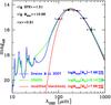 |
Fig. 1 Example of the fits done to estimate the dust mass. Black symbols show stacked fluxes in the bin of the z–Mstar–SFR grid with z = [0.6,1), log Mstar [M⊙] = [10.75,11) and log SFR [M⊙/yr] = [1.4,1.6) The blue line shows the best-fit template from the library of Draine & Li (2007). For a comparison, the green and red curves show the fits with the GRASIL model and with a single-temperature modified blackbody (the latter not fitted to the shortest wavelength flux density), respectively. The dust mass inferred with the three libraries is indicated in the bottom right corner. The three libraries differ in the resulting dust masses by a roughly constant offset, but yield the same trends. |
According to the Draine & Li (2007) model, the interstellar dust is represented as a mixture of amorphous silicate and graphite grains, with size distribution modelled by Weingartner & Draine (2001) and updated as in Draine & Li (2007), mimicking different extinction curves. A fraction qPAH of the total dust mass is contributed by PAH particles (with <1000 C atoms). Although they only provide a minor contribution to the total dust mass, their abundance has an important effect in shaping the galaxy SED at short wavelengths. The majority (a fraction equal to 1 − γ) of dust grains are located in the diffuse ISM and heated by a diffuse radiation field contributed by many stars. This results in a single radiation intensity U = Umin, where U is a dimensionless factor normalized to the local ISM. The rest of the grains are localized in photodissociation regions close to bright stars, and exposed to multiple and more intense starlight intensities (Umin < U < Umax) distributed as a power law (∝U− α).
Following the prescriptions of Draine et al. (2007), we build a library of MW-like models with PAH abundances qPAH in the range 0.47–4.58%, 0.0 < γ < 0.3, α = 2, Umax = 106 and Umin varying between 0.7 and 25. This latter prescription (instead of using Umin ≥ 0.1) prevents the risk of fitting erroneous large dust masses in the absence of rest-frame submillimetre data to constrain the amount of cool dust.
Dust masses are derived by fitting and normalizing the stacked 100-to-500 μm Herschel photometry to this template library. The redshift is fixed to the mean redshift in the bin. The template showing the minimum χ2 is chosen, and the normalization of the fit provides a measure of the dust mass.
In the fitting procedure, we require the stacked fluxes to have at least 3σ significance. In order to have a good sampling of the spectrum, especially on the Rayleigh-Jeans side, most sensitive to the dust mass, we only consider bins with significant flux in at least 3 bands, of which at least one is longward of rest-frame 160 μm (Draine et al. 2007). This enables to account for changes in the dust temperature and makes us confident of the resulting Mdust. 26% of the total number of bins are rejected because of these selections. We visually inspect every single bin to ensure the quality of the fits, and conservatively reject 5 of them (~4%), where the stacked fluxes were not satisfactorily reproduced by the best-fit template. An example of our fitting output can be seen in Fig. 1. The best-fits for all bins in the final sample can be seen in Appendix D.
MIR fluxes are not included in the fit so that the dust mass and SFR estimates are totally independent. As a consistency check, we also computed Mdust by including 24 μm flux densities. The resulting dust masses are in very good agreement with our reference estimates: their mean (median) ratio ( ) is − 0.001 (0.008), with a scatter of 0.07, and the average error bar (see below) is only ~10% lower than without including the 24 μm band. This ratio shows no trends with either stellar mass, SFR or redshift, except a slightly larger scatter at low-z (here rest-frame wavelengths below 100 μm are not sampled in the absence of 24 μm data).
Errors on Mdust are estimated by allowing the stacked photometry to vary within its uncertainty and the redshift to move around the mean value within its standard deviation in the bin. The uncertainty is given by the minimum and maximum Mdust allowed by templates whose probability according to a χ2 test is larger than 32%. All data points whose associated error on Mdust is larger than 1 dex (further ~5% of the available bins) are ignored throughout the analysis, being unable to contribute in understanding the existing trends and only making the plots more crowded without adding information. After all selections, we end up with 122 data points sampling the z–Mstar–SFR grid (see Fig. 4). Dust masses measured in each bin of our grid are listed in Tables A.1.
Our dust masses are in very good agreement with those computed by Magnelli et al. (2014) with the same recipe.
In addition to using the Draine & Li (2007) templates, we also fit our data with a library extracted from the chemospectrophotometric model GRASIL (Silva et al. 1998), tested to reproduce the small galaxy sample of Santini et al. (2010), and with a simple modified blackbody, which assumes a single-temperature dust distribution. For consistency with the Draine & Li (2007) model, we build a modified blackbody with emissivity index β = 2 and absorption cross section per unit dust mass at 240 μm of 5.17 cm2/g (Li & Draine 2001; Draine & Lee 1984). We find that the simplified assumption of single-temperature leads to dust masses which are lower by a factor of ~1.5 compared to those obtained with the more realistic assumption of a multi-temperature grain distribution (in agreement with previous studies, e.g., Santini et al. 2010; Magnelli et al. 2012a,b; Dale et al. 2012; Magdis et al. 2012). Indeed, the attempt of reproducing the Wien side and at the same time the Rayleigh-Jeans side of the modified blackbody spectrum has the effect of overestimating the dust temperature and hence underestimating the dust mass, inversely proportional to the blackbody intensity. However, the recent work of Bianchi (2013) ascribes such disagreement to possible inconsistencies in the treatment of dust emission properties between the two approaches. The GRASIL library fits dust masses larger than the Draine & Li (2007) templates by a factor of 1.5 on average. A direct comparison between the parameters assumed by the two models is not possible, since GRASIL computes dust emission by considering the physical properties of each single grain, instead of assuming an average emissivity. One reason for the discrepancy could be that the optically thin assumption of Draine & Li (2007) is not always verified (even if true, this would not affect our results, which would be simply offset). The GRASIL library adopted, however, has not been tested to work in the absence of submillimeter data. Both the fit with GRASIL and with the modified blackbody provide χ2 values that are a factor of 1.5–2 larger than the Draine & Li (2007) library. For these reasons we decided to use the dust masses obtained from the Draine & Li (2007) templates. We will expand the GRASIL library by enlarging the parameter space to better reproduce our galaxies in a future analysis. In any case, we note that the effect of choosing one dust model or the other only produces an offset, leaving the main trends outlined below almost unchanged.
3.6. Gas metallicities and gas masses
It is possible to take a further step forward with respect to observables directly measurable from our data and compute gas masses by converting dust masses through the dust-to-gas ratio (e.g., Eales et al. 2010). In order to do that, we need to make some assumptions.
We first assume that the gas metallicity is described by the FMR of Mannucci et al. (2010). The FMR is a 3D relation between gas metallicity10, stellar mass and SFR, with a very small scatter (0.05 dex). We assume that it does not evolve from the local Universe to z ~ 2.5, as confirmed by a number of recent works (e.g. Mannucci et al. 2010; Cresci et al. 2012; Nakajima et al. 2012; Henry et al. 2013a,b; Belli et al. 2013). More recently, Bothwell et al. (2013) have shown that the FMR is likely a by-product of a more fundamental relation, between H i gas mass, stellar mass and metallicity (H i-FMR). However, it is beyond the scope of the paper to discuss the origin of this relation. Given the average Mstar and SFR in each bin of our grid, following Mannucci et al. (2010), we compute the gas metallicity from the linear combination μ0.32 = log Mstar − 0.32log SFR, after converting to a Chabrier IMF (as they adopt) both stellar masses (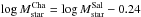 , Santini et al. 2012a) and SFR (log SFRCha = log SFRSal − 0.15, Davé 2008), using their Eqs. (4) and (5) and the extrapolation for low μ0.32 values published in Mannucci et al. (2011). The inferred gas metallicities are in the range 8.58–9.07, with a scatter of 0.14 dex around the mean value of ~8.9.
We note that the FMR has not been tested over the entire SFR range studied in this work on large galaxy samples, so the extrapolation to SFRs larger than ~100 M⊙/yr might in principle result in gas metallicity estimates that are incorrect. Moreover, the detailed shape of the FMR is matter of debate (e.g. Yates et al. 2012; Andrews & Martini 2013). For these reasons, we also tested the robustness of our results by adopting the redshift-dependent mass-metallicity relations published by Maiolino et al. (2008) and verified that all our results are independent of the specific description of the gas metallicity.
As suggested by previous studies, focused either on local (e.g., Draine et al. 2007; Leroy et al. 2011; Smith et al. 2012; Corbelli et al. 2012; Sandstrom et al. 2013), z < 0.5 (e.g., James et al. 2002) or high-z galaxies (e.g., Zafar & Watson 2013; Chen et al. 2013, Cresci et al., in prep.), we consider that a fixed fraction of metals are incorporated in dust. Within the metallicity range probed by our sample, this is true within 0.3 dex at most. Following the parameterization provided by Draine et al. (2007), we assume that the dust-to-gas ratio (δDGR) scales linearly with the oxygen abundance through the constant factor kDGR: 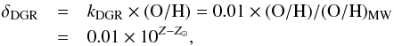 (3)where Z = 12 + log (O/H) is the gas metallicity and Z⊙ = 8.69 is the Solar value (Allende Prieto et al. 2001; Asplund et al. 2009). We find almost identical results from our analysis if we apply the linear relation between log δDGR and gas metallicity inferred by Leroy et al. (2011).
The universality of the depletion factor of metals into dust is outlined by the recent work of Zafar & Watson (2013). According to their analysis, the dust-to-metal ratio can be considered universal, independent of either column density, galaxy type or age, redshift and metallicity. However, De Cia et al. (2013) claim that the dust-to-metal ratio is significantly reduced with decreasing gas metallicity at Z < 0.1 Z⊙ and low column densities. Yet, this should not be a concern for our analysis, since our sample does not include such low-metallicity galaxies. In a more recent paper, Chen et al. (2013) combine constraints on the dust-to-gas ratio of lensed galaxies, GRBs and quasar absorption systems, and find support for a simple, linear universal relation between dust-to-gas ratio and metallicity.
The total gas mass (atomic + molecular, Mgas hereafter) can be computed as 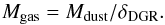 (4)We can finally compute the gas fraction (fgas hereafter) as
 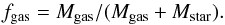 (5)The dust content, typically negligible with respect to the gas and stellar mass components (Mdust ≲ 0.01 Mstar, see below), is ignored in the computation of fgas.
4. Dust scaling relations
In this section we investigate the correlations between Mstar, SFR and Mdust, and their evolution with redshift.
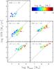 |
Fig. 2 SFR vs. dust mass in different redshift ranges. Galaxies are colour coded according to their stellar mass, as shown by the colour bar. The dashed lines corresponds to the integrated Schmidt-Kennicutt law fitted by Daddi et al. (2010), under the assumption of Solar metallicity (see text) and converted to a Salpeter IMF. |
4.1. Dust content vs. SFR
Figure 2 shows the relation between the SFR and the dust content for galaxies of different Mstar at different redshifts. A correlation between the dust content and the star formation activity is evident at all Mstar and at all redshifts, although with some scatter, while no clear effect is observed with the stellar mass, with bins of different Mstar sometimes overlapping (see also next section).
Before discussing the interpretation of this correlation, we stress here that, not only Mdust and the SFR are estimated from different observed flux densities (Herschel and 24 μm bands, respectively) to avoid any possible degeneracy and with intrinsically independent methods, but also they are not expected to be correlated by definition. The SFR (although in our case measured from 24 μm observations) is in principle linked to the integrated IR luminosity, i.e., it is linked to the normalization of the FIR spectrum. The dust mass comes from a combination of the template normalization and temperature(s), which determines the shape; since the template library that we have used contains multiple heating source components, the dust mass is not trivially proportional to the SFR, though related to it through the dust temperature. To verify that any observed correlation is physical and not an obvious outcome of the relation between correlated variables, we run a simulation that is described in Appendix C, showing that, by starting from a completely random and uncorrelated distribution of dust masses and SFRs, our method does not introduce any artificial correlation.
The correlation observed in Fig. 2 primarily tells us that the dust temperature plays a secondary role. The SFR–Mdust correlation is clearly a consequence of the S-K law, linking the SFR to the gas content. Indeed, as shown in Sect. 3.6, the dust mass is related to the gas mass by means of the dust-to-gas ratio. In other words, we expect the dust mass to be roughly proportional to the gas mass, with the gas metallicity introducing minor effects through the dust-to-gas ratio. Before converting dust masses into gas masses by adopting the appropriate dust-to-gas ratio in the next section, in order to represent the S-K relation on a SFR vs. Mdust plot, for the moment we assume a constant dust-to-gas ratio for all galaxies. By using Eq. (4), the S-K law (in its integrated11 version inferred by Daddi et al. 2010 for local spirals and z ~ 2 BzK galaxies, Daddi et al. 2004) can be written in terms of SFR as a function of Mdust as ![Mathematical equation: \begin{equation} \label{eq:daddi2} \log {\it SFR}[M_\odot/{\rm yr}] = 1.31 \times \log \left(\frac{M_{\rm dust}[M_\odot]}{\delta_{{\rm DGR}\, \odot}} \right) +7.80 , \end{equation}](/articles/aa/full_html/2014/02/aa22835-13/aa22835-13-eq101.png) (6)where the last term includes the factor (1.8 × 10⁻¹⁰) used to convert the total infrared luminosity (the original quantity in the expression given in Daddi et al.) into SFR, as well as the offset of 0.15 needed to convert from a Chabrier to a Salpeter IMF (see Sect. 3.6), and δDGR ⊙ is the dust-to-gas ratio computed from Eq. (3) by assuming a constant Solar metallicity. The dashed line in Fig. 2 shows the inferred S-K relation on the SFR–Mdust diagram.
(6)where the last term includes the factor (1.8 × 10⁻¹⁰) used to convert the total infrared luminosity (the original quantity in the expression given in Daddi et al.) into SFR, as well as the offset of 0.15 needed to convert from a Chabrier to a Salpeter IMF (see Sect. 3.6), and δDGR ⊙ is the dust-to-gas ratio computed from Eq. (3) by assuming a constant Solar metallicity. The dashed line in Fig. 2 shows the inferred S-K relation on the SFR–Mdust diagram.
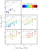 |
Fig. 3 Dust mass vs. stellar mass in different redshift ranges. Symbols are colour coded according to their SFR, as shown by the colour bar. At each Mstar, black open circles mark the bin which lies closest to the MS (in each Mstar interval), and in every case within 0.3 dex from it. The correlations between Mdust and Mstar are rather flat when the data points are separated by means of their SFR. The dashed lines correspond to an amount of dust equal to the maximum metal mass |

Our observational points follow reasonably well the trend expected from the S-K law, with some scatter and a systematic trend (flatter slope) at high-z. We will discuss this in Sect. 5.1, where we also account for the variation of the metallicity (hence the variation of the dust-to-gas ratio as a function of metallicity).
4.2. Dust vs. stellar mass content
We plot in Fig. 3 the dust mass as a function of the stellar mass in bins of redshift. When galaxies are separated according to their SFR (coded with different colours), the correlation found by previous authors (e.g., at low redshift by Bourne et al. 2012) becomes much flatter and sometimes even disappears, hinting that this correlation is at least partly an indirect effect driven by other phenomena. More specifically, the Mdust–Mstar correlation is partly a consequence of the Mdust–SFR correlation, reported in the previous section, combined with the MS, i.e., the relation between SFR and Mstar. When all SFR are combined together, the low mass bins are dominated by low SFR (as a consequence of the MS), which are associated with low Mdust (because of the SFR–Mdust relation). On the other hand, high mass bins are dominated by high SFR and therefore associated with high Mdust. This results into an apparent Mstar–Mdust correlation. To better visualize this effect in studies that combine together all galaxies (i.e., without binning in a grid of SFR and Mdust), in Fig. 3 we have marked with black circles the bins closest to the MS (and in every case within 0.3 dex from it). These are the bins where the bulk of the star-forming galaxy population is concentrated, and, as expected, they show a steeper Mstar–Mdust trend compared to bins of constant SFR.
The dashed line in Fig. 3 represents the expected maximum amount of metals ( , where yZ ≃ 0.014 and
  is the total stellar mass formed, including the final products of stellar evolution12) produced by stars and supernovae explosions, associated with the star formation required to account for the observed Mstar. This is also the maximum amount of dust that can be associated with a given Mstar in a “closed box” scenario and assuming a condensation efficiency in the ejecta close to 100%. More realistically, of these metals only about 30–50% (Draine et al. 2007, grey dotted line in Fig. 3) are expected to be depleted into dust grains. These lines give the maximum amount of dust expected as a function of stellar mass if the galaxy behaves as a “closed box”, and metals are condensed in dust grains with reasonable/high efficiency. Most of the galaxies, in particular the high mass systems, lie below the “closed box” lines. This finding qualitatively agrees with the expectations of theoretical models for the evolution of the dust content: rather flat Mdust–Mstar trends, i.e., decreasing dust-to-stellar mass ratios as the gas is consumed and transformed into stars (see, e.g., Eales & Edmunds 1996; Calura et al. 2008; Dunne et al. 2011). Alternatively, this result might indicate that most of the dust in these systems is lost. In support of this scenario, independently of the dust information, it has been acknowledged that massive galaxies have a deficit of metals, by a factor of a few, relative to what must have been produced in the same galaxies (Zahid et al. 2012), which is ascribed to winds that have expelled metal-rich gas out of these massive galaxies. On the contrary, hints can be seen for low Mstar galaxies (log Mstar [M⊙] ≲ 9.75) to show a high dust mass, close to the maximum “closed box” limit. Recent studies based on SPIRE data in the local and low-z (z < 0.5) Universe support this evidence: large dust-to-stellar mass ratios were reported by Smith et al. (2012), while anti-correlations between the dust-to-stellar mass ratio and stellar mass were observed by Cortese et al. (2012) and Bourne et al. (2012). Due to the necessity of a careful check of optical counterpart associations to IR galaxies with low Mstar, we do not extend this work to such low stellar masses. The dust content in low Mstar galaxies will be investigated by means of a dedicated analysis in a forthcoming paper.
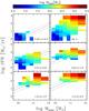 |
Fig. 4 Average dust mass values, as indicated by the colour according to the colour bar, for bins of different SFR and Mstar in different redshift intervals and at all redshifts (upper right panel). Dashed lines represent MS relations of star-forming galaxies as taken from the literature; the local MS is from Peng et al. (2010) (computed using Brinchmann et al. 2004 data), rescaled to a Salpeter IMF, while the relations at higher redshifts are from Santini et al. (2009). Dotted lines represent the ± 1σ (=0.3 dex) scatter of the MS relation. |
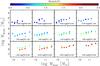 |
Fig. 5 Dust mass vs. stellar mass in panels of different SFR. The symbol colour indicates the mean redshift of each bin, as coded by the colour bar. No evolution with redshift is observed within uncertainties at a given Mstarand SFR. |
4.3. Summary view
To give a global view of these correlations, we show in Fig. 4 the SFR–Mstar plane at different redshifts, where each bin is colour coded according to the associated dust mass. We also show MS relations from the literature (from Peng et al. 2010 at z ~ 0; and from Santini et al. 2009 at high-z). This representation gives a quick overview on the scaling relations existing between Mstar, SFR and Mdust: a weak and sometimes absent trend of Mdust with Mstar and a clear correlation between Mdust and SFR.
It is also worth noting that we observe no evidence for evolution of Mdust across the different redshift ranges at a given Mstarand SFR; the main difference between the various redshift panels in Fig. 4 is simply that they are populated differently. To make this more clear, Fig. 5 shows Mdust as a function of Mstar, in bins of SFR, where the colour coding identifies different redshift bins (note that, as a by-product, Fig. 5 provides further evidence of weak/absent dependence of Mdust on Mstar at a fixed SFR). At a given Mstarand SFR, there is no clear evidence for evolution of Mdust with redshift within uncertainties. We note, however, that we cannot firmly exclude a decrease in Mdust by a factor of 2 from low- to high-z, though this trend is in a few cases reversed. However, observational uncertainties on our data do not allow us to claim any redshift evolution.
It is certainly true that, on average, the overall amount of dust in galaxies at high redshift is higher, as a consequence of the overall higher ISM content in the bulk of high-z galaxies (see Sect. 5.5). As a matter of fact, the normalization of the MS, representing the locus where the bulk of the population of star-forming galaxies lies, does increase with redshift (e.g., Santini et al. 2009; Rodighiero et al. 2010; Karim et al. 2011) and, as a consequence, the dominant galaxy population moves towards larger SFR, hence being characterized by larger dust masses (Fig. 2). However, our results indicate that galaxies with the same properties (same SFR and same Mstar) do not show any significant difference in terms of dust content across the cosmic epochs, at least out to z ~ 2.5. In other words, dust mass in galaxies is entirely determined by the SFR and, to a lesser extent, by Mstar, and it is independent of redshift within uncertainties. Put simply, different cosmic epochs are populated by galaxies with different typical SFR and Mstar values, and hence are characterized by different dust masses.
At fixed SFR, a non evolving Mdust translates into a non evolving dust temperature (Tdust). This does not contradict the results of Magnelli et al. (2014), presenting only a very smooth negative evolution in the normalization of the Tdust-specific SFR (SSFR = SFR/Mstar) relation. They also find a stronger positive evolution in the normalization of the relation between Tdust and the distance from the MS. However, as discussed above, the normalization of the MS itself increases with redshift, hence different SFR–Mstar combinations are probed at different epochs.
Given the lack of any significant redshift evolution in the dust mass at fixed Mstarand SFR, it is meaningful to represent all redshift bins on the same SFR–Mstar plane (upper right panel of Fig. 4) to provide an overview of the dust content over a wider range of Mstar and SFR. Here the dust mass is computed by averaging the values at different redshifts. This further confirms the trends already outlined (Mdust depends strongly on the SFR and weakly on Mstar), over a wider dynamic range.
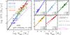 |
Fig. 6 Left panel: relation between SFR and gas mass. The colour code indicates different redshift intervals, as shown by the legend in the upper left corner. The black boxes mark bins that lie in the starburst region according to Rodighiero et al. (2011). The solid thick black line is the power law fit to all data, and the best-fit relation is reported in the lower right corner. The dashed and dotted grey lines show the integrated Schmidt-Kennicutt relations fitted by Daddi et al. (2010) and Genzel et al. (2010), respectively, on normal star-forming galaxies (lower curves) and on local ULIRGs and z ~ 2 SMGs (upper curves). Curves from the literature are converted to a Salpeter IMF. Magenta dashed-dotted lines indicate constant star formation efficiencies (i.e., constant depletion times) of 1 (lower curve) and 10 (upper curve) Gyr-1. Right panels: relation between SFR and gas mass in different redshift bins, indicated in the upper left corner of each panel. Symbol styles and colours are as in the left panel. The coloured solid curves are the power law fits to the data, and the numbers in the lower right corner indicate the best-fit slope (upper) and intersection at log Mgas [M⊙] = 10 (lower) (see Eq. (7)). The dashed-triple dotted lines show the best-fit relation given in Eq. (8) calculated at the median redshift in each panel. |
5. The evolution of the gas content in galaxies
We investigate here the relation between the gas content and the SFR, as well as the evolution of the gas fraction, with the aim of understanding the processes driving the conversion of gas into stars in galaxies throughout the cosmic epochs. We recall that gas masses are inferred from dust mass measurements by assuming that the dust-to-gas ratio scales with the gas metallicity, and by computing the latter by means of the FMR of Mannucci et al. (2010) (see Eqs. (3), (4)). We verified that all the results presented below are almost unchanged if the redshift-dependent mass-metallicity relation of Maiolino et al. (2008) is used instead of the FMR.
5.1. The star formation law
We plot in Fig. 6 the values of SFR as a function of gas mass. The colour code identifies bins of different redshift. For the sake of clarity, the data points at the different redshifts are also plotted on separate panels on the right side. This figure is analogous to Fig. 2, except that Mgas, plotted here instead of Mdust, takes into account the dependence of the gas metallicity with stellar mass and SFR (see Sect. 3.6). This, however, introduces only a minor effect (the gas metallicity changes less than a factor of 2–3, while the dust mass spans 2–3 orders of magnitude). The relation shown in Fig. 6 can be referred to as the integrated S-K law, meaning that gas masses and SFRs are investigated values rather than their surface densities, as in the original S-K law, where the SFR surface density is related to the gas surface density by a power law relation. We fit the data points with the relation  (7)A standard χ2 fit cannot be performed on our data given the asymmetric error bars. Therefore, all over our work, we apply a maximum likelihood analysis by assuming rescaled log-normal shapes for the probability distribution functions of the variables with the largest uncertainties (log Mgas in this case) and by ignoring the uncertainties on the other variables. By fitting the total sample we obtain
  and
and  , where a bootstrap is performed to compute the parameter 1σ errors. The best-fit relation is represented by the black solid line in the left panel of Fig. 6. However, due to inhomogeneous sampling in SFR at different redshifts, the fit might suffer from biases in case there is an evolution in the slope or normalization of the relation. To investigate such effects, we also separately fit the points in each individual redshift bin (coloured solid lines in the right panels of Fig. 6). The inferred slopes monotonically decrease with redshift from
  in the local Universe to
  at z ~ 2, while the normalizations increase from
  to
to  . The best-fit parameters are given in the bottom right corner of each panel of Fig. 6.
By following the theoretical model of Davé et al. (2011, 2012) and the observational results of Tacconi et al. (2013), we also attempt to fit our data points with a relation that has a single redshift-independent slope and normalization slowly evolving with redshift, i.e., yielding a cosmological scaling of the depletion time (=Mgas/SFR):  (8)The best-fit parameters are
  ,
,  and
and  . The dashed-triple dotted lines in the right panels of Fig. 6 show the inferred relation at the median redshift in each bin. However, this function provides a worse fit to the data in terms of probability of the solution as computed from the likelihood, with respect to Eq. (7).
In both cases, the evolution of the relation with redshift may be partly caused by mixing different stellar masses, whose contribution strongly depends on the SFR and redshift because of the evolution of the MS relation.
5.1.1. Comparison with previous works
The inferred relations agree, on average, well with those fitted by previous work based on CO measurements for normal star-forming galaxies (Daddi et al. 2010, lower dashed grey line in Fig. 6, see also Eq. (6); and Genzel et al. 201013, lower dotted grey line), although we fit a steeper slope on all data points. The values of the best-fit slopes are independent of the galaxy population (i.e., consistent fits are found if starburst galaxies are removed, see below), and of the recipe adopted for the gas metallicity (i.e., consistent results are obtained if we assume no dependence on the SFR and redshift evolution of the mass-metallicity relation). Anyhow, the broad agreement with previous studies for the majority of galaxies (see below) and the small dispersion (the average absolute residual is ~0.15 dex in terms of log Mgas) shown by our data points are impressive, especially given the completely different and independent approaches used to derive the star formation law. This confirms the reliability of our approach of deriving gas mass estimates from dust mass measurements.
We remind the reader that the dust method is supposed to trace both the molecular and atomic gas (the dust-to-gas conversion factor adopted refers to the total gas mass). Bigiel et al. (2008) have measured steeper slopes for the star formation laws in local galaxies when both the molecular and atomic gas components are considered. This may explain our steeper slopes compared to previous CO-based studies (e.g., Genzel et al. 2010; Tacconi et al. 2013). However, the fair agreement with the Daddi et al. (2010) relation (inferred from CO observations, a proxy for molecular hydrogen) is suggesting that, if the latter is correct, the bulk of the gas in these galaxies is in the molecular phase, which is reasonable given that most of these galaxies are vigorously forming stars and will have high pressure ISM conditions (see also Leroy et al. 2009; Magdis et al. 2012). The steeper slopes found at low redshift may be determined by a larger atomic-to-molecular gas ratio at low than at high-z (see below). Another possibility to explain this is the trend for the MS template of Elbaz et al. (2011) to slightly underpredict the SFR in the absence of Herschel data for bright galaxies at high-z (SFR > 100 M⊙/yr, see Fig. B.1 and Berta et al. 2013); by moving the data points with the largest SFR towards lower SFR values, this effect might be responsible for the shallower slope measured at high redshift. However, as it can be seen in Fig. B.1, this effect is not larger than 0.1–0.2 dex, and is therefore unlikely to affect our other results (on the other side, the fitted slope of the S-K law may be sensitive to small offsets in the SFR). As a matter of fact, the results presented in this paper are very similar if other IR templates (e.g., Dale & Helou 2002) are used to measure the SFR from 24 μm fluxes or from all Herschel bands. Finally, steep slopes for the global star formation law may be explained by the results of Saintonge et al. (2013), who claim that the gas-to-dust ratio may be 1.7 times larger at z > 2 than observed locally. This, however, would only marginally affect our highest redshift bins, whose mean redshift value is around 2.
Note that the fact that the slope of the global S-K relation, as well as those at z < 0.6, are steeper than unity implies that galaxies with high SFRs have higher star formation efficiency (defined as SFE = SFR/Mgas, equal to the inverse of the depletion time), even if they are regular, MS galaxies. The magenta dash-dotted lines in Fig. 6 trace the loci with SFE = 1 Gyr-1 (lower line) and SFE = 10 Gyr-1 (upper line). As a consequence of the super-linear slope of the S-K relation, moderate star-forming galaxies (SFR ~ 1 M⊙/yr) have a SFE approaching 1 Gyr-1, while strongly star-forming galaxies (SFR ~ several 100 M⊙/yr) have a SFE approaching 10 Gyr-1, implying gas depletion timescale of a few times 100 Myr. However, the SFE is more properly defined as the ratio of the SFR over the molecular gas content. Therefore, another possibility to interpret our result is that the SFR/Mmolgas stays the same, and the atomic gas content decreases in strongly star-forming galaxies, or, in other words, the latter have a larger molecular to atomic fraction. This would be confirmed by the results of Bauermeister et al. (2010), who observe little evolution in the cosmic H i density, while the molecular component is expected to positively evolve out to the peak of cosmic star formation (z ~ 2–3, Obreschkow & Rawlings 2009; Lagos et al. 2011; Popping et al. 2013).
5.1.2. The star formation law for starburst galaxies
Symbols marked with a black box in Fig. 6 correspond to bins which lie in the starburst region of the SFR vs. Mstar diagram according to the selection of Rodighiero et al. (2011). They select starburst galaxies as sources deviating from a Gaussian logarithmic distribution of the SSFR, having SSFR four times higher than the peak of the distribution (associated to MS galaxies). Given the average scatter of 0.3 dex of the MS (Noeske et al. 2007), these galaxies are located >2σ above the MS (see Fig. 4). The effectiveness of this SSFR criterion in selecting starburst galaxies is confirmed by semi-analytical models where starburst events are triggered by galaxy interactions during their merging histories (Lamastra et al. 2013a). Galaxies from our sample located in the starburst regions do seem to follow the same star formation law as all other galaxies. We note that the selection of starburst galaxies above is based on the knowledge of the MS from the literature, rather than computed directly on the present sample. However, this does not affect our conclusions. Indeed, the observed correlation between SFR and Mgas is tight enough that, even in case of small variations in the location of the MS, sources selected as starburst would still follow the same relation (for example, results are unchanged if the MS from Whitaker et al. 2012 is used, despite its shallower slope). Unless indicative of a larger fraction of atomic gas in starbursts, this result is in contrast with what suggested by previous studies, mostly based on CO emission (e.g., Daddi et al. 2010; Genzel et al. 2010; Saintonge et al. 2012; Magdis et al. 2012; Sargent et al. 2013). The latter studies find a normalization of the star formation law ~10 times higher for starburst galaxies, implying a larger SFE. In any case, since the slope of the relation that we infer is larger than unity (except at z > 0.6), our result does not imply a low efficiency in converting gas into stars for galaxies located in the starburst region (see next section): starburst galaxies do have, on average, larger star formation efficiency (i.e., shorter depletion times) than the bulk of star-forming galaxies (typically at lower SFR).
We note that our work does not sample the most extreme objects lying at the bright tail of the SFR distribution (all but one of the bins selected as “starbursts” are located between 2σ and 3σ above the MS). Physical properties of very extreme sources, such as local ULIRGs or high-z SMGs, are not always compliant with local-based expectations (see, e.g., Santini et al. 2010) and need to be treated with ad-hoc techniques (for example, Magdis et al. 2012 claim the need of submm data to reliably estimate dust masses of SMGs). Moreover, larger statistics is needed. We will therefore study such extreme sources in a future work.
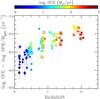 |
Fig. 7 Redshift evolution of the star formation efficiency (SFE, or inverse of the depletion time). Different colours refer to different SFRs, as shown by the colour bar. Black boxes are as in Fig. 6. |
5.2. The evolution of the star formation efficiency
The slope of the integrated S-K relation inferred from our data is generally steeper than unity (except possibly at high redshift). As a consequence, the SFE for high redshift galaxies, which are also on average more star-forming, is higher than for local galaxies, or, equivalently, the depletion time is shorter (we here assume negligible atomic fraction for all galaxies, but see comment in Sect. 5.1.1). This is illustrated in Fig. 7, where the SFE is plotted as a function of redshift, and where an increase in the SFE with redshift is indeed observed, although with large scatter. Due to degeneracy between SFR evolution and redshift it is not clear whether the increase in the SFE with redshift truly reflects a cosmic evolution of the SFE, i.e., galaxies of a given SFR convert their gas into stars more efficiently at high-z, or it is simply a by-product of the slope of the S-K relation convolved with the higher SFR characterizing high-z galaxies (higher normalization of the MS). In Fig. 7 galaxies with different SFRs are plotted with different colours, in an attempt to break the degeneracy between redshift and SFR. Galaxies with similar SFR show no clear internal evolution with redshift. However, due to observational biases (difficulties in observing faint sources at high-z as well as paucity of rare bright sources in small volumes at low-z) the redshift spanned by each of these sets of points is very narrow, and the dispersion very high, hence we cannot rule out a real, intrinsic evolution of the SFE in galaxies (at a given SFR). We will investigate this issue in more detail in another paper (Santini et al., in prep.).
In any case, regardless of whether the evolution of the SFE is an intrinsic redshift evolution or driven by the slope of the S-K relation and the evolution of the SFR, the net result is that the bulk of the galaxy population (i.e., galaxies on the MS) at high redshift (z ~ 2) do form stars with a SFE higher by a factor of ~5 than the bulk of the population of local star-forming galaxies. This evolution is roughly consistent with the evolution of the dust mass-weighted luminosity (LIR /Mdust, proportional to the SFE except for a metallicity correction) found by Magdis et al. (2012) (a factor of ~4 from z ~ 0 to z ~ 2) and only slightly steeper than the evolution of the depletion time (a factor of ~3 in the same redshift range) observed by Tacconi et al. (2013), likely due to the steeper S-K law inferred by us compared to their work.
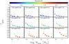 |
Fig. 8 Gas fraction vs. stellar mass in panels of different average SFR. The colour of the symbols reflects the mean redshift of each bin, as indicated by the colour bar. No evolution with redshift is observed, within uncertainties, at given SFR and Mstar. Grey dashed curves are the best-fits to the data assuming the functional shape in Eq. (9). Best-fit parameters for each SFR interval are summarized in Table 1. |
5.3. The evolution of the gas fraction
Figure 8 shows the gas fraction as a function of the stellar mass, colour coded according to the redshift, in panels of different SFR. The gas fraction decreases with the stellar mass, as expected by the gas conversion into stars in a closed-box model, and increases with the SFR, as a consequence of the S-K relation (see also the results of Magdis et al. 2012; and those of the PHIBSS survey presented in Tacconi et al. 2013). Most interesting is the lack of evolution of the gas fraction with redshift, once galaxies are separated according to their Mstar and SFR values. Given the assumptions made to compute the gas mass, hence gas fractions, this finding is the result of the lack of (or marginal) evolution of the dust content in bins of fixed Mstarand SFR (see Fig. 5), combined with a minor contribution from the gas metallicity evolution with Mstar and SFR (the FMR, Mannucci et al. 2010).
From the lack of redshift evolution of the gas fraction at fixed SFR and Mstar, it follows that galaxies within a given population (identified by a combinations of SFR and Mstar), convert gas at the same rate regardless of redshift, i.e., the physics of galaxy formation is independent of redshift, at least out to the epochs probed by our work. This is essentially a consequence of the unimodal inferred S-K relation, but Fig. 8 shows the result more neatly by also slicing the relation through the dependence on stellar mass, which is the third fundamental parameter. We note that this does not contradict the evolution of the SFE observed in Fig. 7, where different stellar masses and SFR are mixed together and where selection effects cause the different SFR bins to be populated differently at different redshifts (hence the average at each redshift is certainly biased).
In summary, our result implies that, at fixed stellar mass, the SFR is uniquely driven by the gas fraction via the star formation law. In other words, if two among SFR, Mstar and Mgas are known, the third property is completely determined and does not depend on redshift. This provides a powerful tool to overcome the observational difficulties related with the measurement of gas or dust masses and analyse the gas content for much larger samples of galaxies.
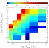 |
Fig. 9 Average gas fractions, as indicated by the upper colour bar, in bins of Mstar and SFR. |
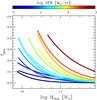 |
Fig. 10 Parameterization of the gas fraction as a function of stellar mass at all redshifts in different SFR intervals, using the functional shape given in Eq. (9) (see text). Curves of different colours refer to different SFR bins, as shown by the colour bar. |
5.4. The fundamental fgas–Mstar–SFR relation
Given the lack of evolution with redshift observed for the gas fraction once galaxies with the same Mstarand SFR are considered, we can combine all redshift bins together to increase the statistics and infer more clearly the trend of fgas as a function of Mstar in different SFR intervals. Figure 9 shows the resulting global dependence of the gas fraction (given by the colour coding) on the SFR–Mstar plane. In each SFR interval, we fit the data points with a linear relation in the logarithmic space:  (9)We shift the stellar masses, placing them across zero, in order to de-correlate the slope and offset parameters in the linear fit result. The best-fit parameters are given in Table 1, and the best-fit curves are shown by the dashed grey lines in Fig. 8 and also by the solid coloured lines in Fig. 10, which provides a direct comparison at different SFRs. We note that the functional form adopted above does not necessarily have physical meaning: it is a purely phenomenological representation of the data to better visualize the observed trends and to interpolate the three physical quantities for later use of this 3D relation.
The three-dimensional fgas–Mstar–SFR relation shown in Fig. 10 is a fundamental relation that does not evolve with redshift, at least out to z ~ 2.5. Galaxies move over this surface during their evolution.
Figure 11 shows a 3D representation of such a relation. Further investigation of this 3D relation and its physical interpretation goes beyond the scope of this paper, and will be discussed in a future work, as well as the relation between the independent quantities Mgas, Mstar and SFR. Here we only emphasize that the redshift evolution of the S-K law seems to disappear once sources are divided in bins of Mstar. Indeed, the redshift evolution of the SFE illustrated in Fig. 7 is most likely a consequence of the fact that high-z bins are mostly populated by galaxies with high SFR, which are characterized by high SFE, as a consequence of the super-linear slope of the S-K relation.
We note that the fundamental relation presented here is indeed a physical result, rather than just a way of looking at the redshift evolution through the evolution of another parameter (e.g., SFR). In other words, the inclusion of the SFR or stellar mass as parameters is not masking a true underlying redshift evolution. As a matter of fact, no similar relation is obtained if redshift is replaced to either SFR or Mstar.
5.5. The evolution of the gas fraction among main sequence galaxies
The finding that the fundamental fgas–Mstar–SFR relation does not evolve with redshift does not contradict the claimed redshift evolution of the gas fraction in galaxies (e.g., Daddi et al. 2010; Tacconi et al. 2010, 2013; Magdis et al. 2012). Indeed, as already mentioned, galaxies do not uniformly populate this 3D surface. As they evolve, the bulk of star-forming galaxies populate different regions of this surface, as a consequence of gas accretion, gas consumption by star formation and gas ejection. The projection of such a distribution onto the Mstar–SFR plane yields the MS and its evolution with redshift.
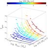 |
Fig. 11 Representation of the 3D fundamental fgas–Mstar–SFR relation. The colour code indicates the average SFR of each bin. The best-fit relations shown in Fig. 8 are overplotted. |
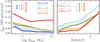 |
Fig. 12 Left: gas fraction vs. Mstar at different redshifts (in different colours according to the legend) for main sequence (MS) galaxies. Right: gas fraction vs. redshift at different Mstar (in different colours according to the legend) for MS galaxies. Curves are obtained by interpolating the fgas parameterizations reported in Fig. 10 and Table 1 and the MS relations (see text for details) at Mstar above the minimum sampled Mstar common to all SFR bins. Mean uncertainties on gas fraction associated to MS galaxies in each redshift (left) or stellar mass (right) bin are plotted. |
As suggested by various models, the evolution of galaxies is likely driven by the evolution of their gas content. The evolution of the MS is likely a by-product of the gas content through the S-K relation, or more generally through the fundamental fgas–Mstar–SFR relation illustrated above. While the evolution of the MS has been constrained by several observations, its driving process, which is the evolution of the gas content, is still loosely constrained. We can however exploit the observed evolution of the MS to infer the evolution of the gas fraction of the population of galaxies dominating star formation at any epoch, by exploiting the fundamental fgas–Mstar–SFR relation.
We take advantage of the mathematical representation of the gas fraction as a function of Mstar at given SFR shown in Fig. 10, and we linearly interpolate these relations onto a finer SFR grid. We then adopt the MS relations reported in Fig. 4 and linearly interpolate them onto a fine redshift grid. At a given Mstar and redshift, we use the MS relation to compute the expected SFR, according to which we select the appropriate fgas parameterization.
The resulting evolution of fgas with stellar mass at different redshifts (colour coded) is shown in the left panel of Fig. 12. The orthogonal plot, i.e., the redshift evolution of fgas for different stellar masses (colour coded), is shown in the right panel of Fig. 12. These plots illustrate how the “bulk” of the star-forming galaxy population at various epochs populates the 3D fundamental fgas–Mstar–SFR relation as a function of redshift. Essentially, for a given stellar mass, the average gas content of star-forming galaxies increases steadily with redshift, at least out to z ~ 2.5. The increase rate is steeper for low mass galaxies with respect to massive galaxies. Galaxies with log Mstar [M⊙] ~ 10.6 reach fgas ~ 0.25 around the peak of cosmic star formation at z ~ 2.5, while massive galaxies, with log Mstar [M⊙] ~ 12 reach a gas fraction of only 0.18 at the same cosmic epoch. This behaviour is consistent with a downsizing scenario (Cowie et al. 1996; Fontanot et al. 2009), where massive galaxies have already consumed most of their gas at high redshift, while less massive galaxies have a larger fraction of gas (though more complex scenarios resulting from the interplay of inflows, outflows and star formation are not excluded). Further, in massive galaxies the gas fraction decreases more steeply moving towards lower redshift (with respect to low mass galaxies) and their gas evolution flattens to low values at z ≲ 1.3. Instead, low mass galaxies show a shallower and more regular decrease of the gas content, moving towards lower redshifts. Both trends are further indications of downsizing.
The fgas values are somewhat lower by a factor of ~1.5–2 on average (after accounting for the IMF conversion) than inferred by the high-z CO survey of Tacconi et al. (2013). A similar or even larger mismatch with CO-based results was found by Conselice et al. (2013), who compute gas fractions from SFR and galaxy sizes by inverting the S-K law. We ascribe the discrepancy to the combination of the various uncertainties associated with CO studies and with our method. In addition, the underestimate by ≃50% of the dust mass of unresolved sources found by Galliano et al. (2011) may also explain the lower values found by us. The gas fractions derived by us are also lower by a factor of ~2 than those published by Magdis et al. (2012), who adopt a similar method. This might be caused by cosmic variance effects: based on the two GOODS fields only, the analysis of Magdis et al. (2012) may be affected by statistical uncertainty. The inclusion of COSMOS data provides much improved statistics that is crucial in stacking analyses. Indeed, the stacking result is closely related to the number of stacked sources. Even if COSMOS is shallower than the deep GOODS fields, SPIRE observations, on which dust masses mostly rely, are confusion limited. Therefore, the statistics is strongly dominated by COSMOS. To verify whether cosmic variance effects could be responsible for such disagreement, we repeated our analysis by only including the two GOODS fields. Given the limited statistics, we end up with only 10 data points. We compared these with our gas fractions and found that in 30% of the cases the former are indeed larger by a factor of 2–2.5, while the rest of the points are consistent within their error bars. Finally, we note that the disagreement with previous works is reduced when the GRASIL model is adopted instead of Draine & Li (2007).
5.6. Comparison with theoretical predictions
The evolution of the gas fraction is a powerful observable to test the various physical processes at play in galaxies and implemented by theoretical models, such as star formation, gas cooling and feedback. Here we compare our findings for the evolution of the gas fraction with the expectations of the semi-analytical model of galaxy formation developed by Menci et al. (2008, and references therein). This connects, within a cosmological framework, the baryonic processes (gas cooling, star formation, supernova feedback) to the merging histories of the dark matter haloes, computed by means of a Monte Carlo simulation. Gas is converted into stars through two main channels: a steady (or quiescent) accretion mode, in which the cold gas in the galaxy disk is converted into stars on long timescales (~1 Gyr), and an interaction-driven mode, where gas destabilized during major and minor mergers and fly-by events is converted into stars on shorter timescales (~107 yr; see Lamastra et al. 2013a,b, for a more detailed description). AGN activity triggered by the same galaxy interactions and the related feedback processes are also included.
The predicted gas fraction as a function of stellar mass and redshift is shown in Fig. 13. On the same figure we report the extrapolations for MS galaxies based on our observations already shown in Fig. 12. As discussed above, MS galaxies represent the bulk of the galaxy population and can be directly compared to the darkest contours, enclosing the region occupied by most of the galaxies.
Observations are generally well reproduced by the theoretical model, although with some systematic deviations. The trends with both stellar mass and redshift are recovered, as well as the downsizing expectations: a strong evolution can be noticed in low mass galaxies (Mstar ≲ 1011 M⊙/yr), which are gas-rich out to z ~ 1 (bottom right panel), while progressively more massive galaxies have already consumed their gas at this epoch (upper right panel). While a very good agreement is recovered for all stellar masses at high redshift (z ~ 2, upper-left panel), the predicted evolution of the gas fraction is more regular than observed at intermediate redshifts, with a gas fraction in log Mstar [M⊙] ≲ 11.5 galaxies of ~0.2 at z ≳ 0.6, around twice the observed value (central left panels). The overall systematic gas richness of model galaxies compared to the observations relates to the long-standing problem of theoretical models in reproducing the galaxy stellar mass functions at high redshift. Indeed, the number of massive galaxies is underpreticted by the models (e.g. Fontanot et al. 2009; Santini et al. 2012a), consistently with the inefficiency of the gas conversion and mass buildup processes in the distant Universe. Once gas consumption has started, it is not effectively suppressed at late stages. Indeed, the model predicts a fraction of very massive (log Mstar [M⊙] ≳ 11.5) galaxies which are still gas-rich at z < 1, at variance with what observed (lower- and central-left panels and top-right one). Although it can be partly ascribed to fluctuations in the fgas distribution generated by the low number statistics of such high Mstar galaxies, this behaviour is a manifestation of a known problem common to all theoretical models, in which the suppression of the star formation activity is still inefficient, despite the feedback processes at work. This is related to the difficulties in reproducing the fraction of red passive galaxies (Fontana et al. 2009).
For all these reasons, the comparison of observed and predicted gas fraction is of major importance to constrain the physical processes implemented in models of galaxy formation and evolution. A more detailed and complete comparison with theoretical expectations will be tackled in a future work.
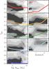 |
Fig. 13 Predicted evolution of the gas fraction according to the semi-analytical model of Menci et al. (2008). The five filled contours indicate the fraction of galaxies having a given fgas at a fixed Mstar (left panels) and redshift (right panels). The trends for MS galaxies extrapolated from our observations (shown in Fig. 12) are overplotted. |
6. Summary
We have used Herschel data from both PACS and SPIRE imaging cameras to estimate the dust mass of a large sample of galaxies extracted from the GOODS-S, GOODS-N and COSMOS fields. To explore a wide range of galaxy properties, including low mass and moderate star-forming galaxies, we have performed a stacking analysis on a grid of redshifts, stellar masses and SFR, and considered average values. With these outputs we have studied the scaling relations in place between the dust content of galaxies and their stellar mass and SFR at different redshifts, from the local Universe out to z = 2.5. Our main results are the following.
-
No clear evolution of the dust mass with redshift is observed at a given SFR and stellar mass. Although there is a global redshift evolution of the dust content in galaxies, as a consequence of the increased ISM content at high-z, our findings indicate that galaxies with the same properties (same SFR and same Mstar) do not show any significant difference in terms of dust content across the cosmic epochs, at least out to z ~ 2.5. In other words dust mass in galaxies is mostly determined by SFR and Mstar and is independent of redshift.
-
The dust content is tightly correlated with the star formation activity of the galaxy. This correlation is in place at all values of Mstar probed and at least out to z ~ 2.5. Under the assumption that the dust content is proportional to the gas content (with a factor scaling with the gas metallicity), the observed correlation is a natural consequence of the Schmidt-Kennicutt (S-K) law.
-
The correlation between the dust and stellar mass observed by previous studies (which averaged together all SFR) becomes much flatter or even disappears when taken at a fixed SFR. The Mdust − Mstar relation is at least partly a result of the Mdust–SFR correlation combined with the main sequence (MS) of star-forming galaxies.
-
We fit a power law relation between the SFR and the gas mass, in good agreement with that previously obtained by Daddi et al. (2010), and also broadly consistent with the results of Genzel et al. (2010). This agreement is remarkable, given the completely different approach between our study and the two works above based on CO measurements. We find that all galaxies follow the same star formation law (integrated S-K law), with no evidence of starbursts lying on an offset relation, though our sample lacks the most extremely starbursting sources (such as local ULIRGs and their analogues at high-z). The slope of this relation is on average steeper than unity, implying that strongly star-forming galaxies have higher star formation efficiency (SFE, i.e., the inverse of the depletion time), or shorter depletion time. We also find a mild, but significant evolution of the S-K law with redshift.
-
We observe an evolution of the SFE with redshift, by about a factor of 5 from z ~ 0 to z ~ 2.5. This applies to the bulk of the galaxy population dominating star formation at each epoch. However, it is not clear whether such evolution is an intrinsic redshift evolution or is simply a consequence of sampling more star-forming galaxies at high redshift combined with the slope of the integrated S-K relation being on average steeper than unity.
-
The measured gas fraction decreases with stellar mass and increases with SFR, as expected. However, when considering bins of given stellar mass and SFR, the gas fraction does not show any redshift evolution, at least out to z ~ 2.5. This primarily results from the non-evolution of the dust mass (within uncertainties), with gas metallicity effects only providing a second-order contribution. The 3D relation between fgas, Mstar and SFR is a fundamental relation that holds at any redshift. It provides a powerful tool to overcome the observational difficulties related with the measurement of gas or dust masses and to analyse the gas content for much larger samples of galaxies. Galaxies populate such a 3D fundamental fgas–Mstar–SFR relation in a different way throughout the cosmic epochs. The projection of galaxies on the 3D fundamental relation onto the Mstar–SFR plane gives the MS and its evolution with redshift.
-
We “de-project” the MS galaxies, at various cosmic epochs, onto the 3D fundamental fgas–Mstar–SFR relation, to infer the evolution of the gas fraction of “typical” star-forming galaxies as a function of redshift. A clear redshift evolution from z ~ 0 to z ~ 2.5 in the gas fraction is observed for MS galaxies. The evolution of the gas content in massive (Mstar ≳ 1011 M⊙) galaxies is steep between z ~ 2.5 and z ~ 1.3 and flattens to low fgas values at lower redshifts. Low mass Mstar ≲ 1011 M⊙ galaxies show a less steep and more regular decrease of the gas fraction from z ~ 2.5 to z ~ 0. These trends are in agreement with the downsizing scenario for galaxy evolution, and they are on average well reproduced by the theoretical expectations of the semi-analytical model of Menci et al. (2008), despite a systematic larger gas richness compared to our data.
Online material
Appendix A: Statistics on the z–Mstar–SFR grid
We report in Tables A.1 the number of sources in each z–Mstar–SFR bin and the associated average dust mass.
Number of sources (upper number in each cell) and average dust mass (lower number in each cell) in each z–Mstar–SFR bin.
Appendix B: Reliability of the SFR estimates
To verify the reliability of the 24 μm-based SFR tracer (SFR24), we compare it with the SFR measured by fitting the average FIR stacked flux densities (SFRFIR). We fit these flux densities with the Dale & Helou (2002) IR template library to infer an estimate of the total IR luminosity, and account for the unobscured SFR by taking into account the average rest-frame UV luminosity in the bin uncorrected for extinction (see Sect. 3.2 for more details). The same results are found if the MS template of Elbaz et al. (2011) is used instead of the Dale & Helou (2002) library. In the left panel of Fig. B.1 we compare the average SFR24 in each bin of the grid with the average SFRFIR. The two SFR measurements nicely agree with each other with the only noticeable exception of the lowest redshift bin, making us confident of the method adopted. The small offset observed at low-z does not significantly affect our results.
We also repeated the same test by making use of a “ladder of SFR indicators” (SFRladder, e.g. Wuyts et al. 2011a) as input for the grid production. Such a “ladder” approach combines different SFR estimates by using the best available choice for each galaxy. More specifically, a Herschel-based SFR is used for galaxies detected by PACS or SPIRE, the 24 μm-based tracer
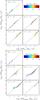 |
Fig. B.1 Left: comparison between the 24 μm-based SFR used in the analysis (x-axis) and the SFR measured by fitting the average FIR stacked flux densities for each bin of the grid (y-axis). The colour code indicates the mean stellar mass in each bin. Right: same as the left panel, but FIR-based SFR are compared to the SFR measured by means of a “ladder” approach (see text). |
is adopted for galaxies undetected by Herschel but detected by MIPS, and the output of the optical-UV SED fitting described in Sect. 3.1 is used for galaxies undetected at IR wavelengths. Most importantly, this approach has the advantage of increasing the number of galaxies for which a SFR estimate is available and enlarging the SFR dynamical range. However, as evident from the right panel of Fig. B.1, the scatter with respect to SFRFIR is larger than in the previous case. Moreover, the correlation between SFRladder and SFRFIR flattens at low SFR and z > 0.2, exactly at the SFR regime where in principle the “ladder” approach provides an improvement over the 24 μm-based SFR. One possibility to explain the flat behaviour at low SFR (below a redshift-dependent threshold) shown in the right panel of Fig. B.1 is to ascribe it to failures in the associations of optical counterparts for the extremely faint IR galaxies or blending issues mostly affecting the faintest galaxies during the stacking procedure. Alternatively, dust heating by old stellar population might also be responsible for the enhanced IR flux at low SFR. However, investigating the reasons of such disagreement is beyond the scope of the present work. Based on the tests performed, we decide to use SFR24 as a SFR tracer, at the expenses of reducing the SFR dynamical range, in order not to run the risk to introduce systematics in the analysis.
Appendix C: Simulation to test against possible degeneracies in the SFR–Mdust correlation
We run a simulation to verify that the trend observed between the SFR and the dust mass (Fig. 2) is real and not a trivial outcome of the fact that both physical variables are related to the FIR peak of the galaxy SED. Indeed, while the SFR is simply proportional to the integrated light in the dust emission peak, the dust mass depends not only on the normalization of the spectrum but also on the temperature of the grains, which determines its shape.
The aim of the simulation is to verify whether an initially scattered and uncorrelated distribution of mock SFR and Mdust gives rise to a correlation when the two quantities are recomputed according to our methods. To do that, we consider a set of GRASIL templates, each associated to a dust mass (Mdust INPUT) and to a SFR (SFRINPUT). The latter is computed by integrating the template from 8 and 1000 μm and multiplying by the calibration factor 1.8 × 10⁻¹⁰ (see Sect. 3.2). In order to sample a wide region of the SFR–Mdust parameter space, we multiply each SFR–Mdust pair by a normalization factor. This corresponds to multiplying the associated SED, since both parameters scale with the SED normalization. We consider a range in SFR and Mdust which mimic that observed in one of the redshift interval most populated by our data, i.e., 0.6 < z < 1. The resulting SFR–Mdust distribution is shown in the left panel of Fig. C.1.
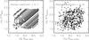 |
Fig. C.1 Distribution of mock SFR and Mdust in input (left panel) and output (right panel) of the simulation described in text. The measure of the SFR and Mdust does not introduce a correlation in an initially uncorrelated distribution. The value of the Pearson coefficient is printed in both cases. |
We redshift each mock galaxy to a random redshift within the 0.6-1 interval, and interpolate the associated spectrum with the MIPS 24 μm and Herschel 100–500 μm filters. To mimic the real case, we perturb such mock flux densities by adding a noise randomly extracted from the observed noise distribution in each band. We then measure the SFR (SFROUTPUT) and Mdust (Mdust OUTPUT) for each mock galaxy exactly as we have done for the real data. Consistently with what described in Sect. 3.5, we reject sources not compliant with our requirements to ensure reliable dust mass estimates. The resulting measurements are shown in the right panel of Fig. C.1 and show no evidence for any correlation between SFR and Mdust. The absence of any correlation induced by our measures is statistically confirmed by the values of the Pearson coefficients on the input (0.11) and output (0.19) data point distributions. This simulation illustrates that the correlations between Mdust and SFR is not an artefact of the method, but is physical (i.e., the result of the S-K law).
Appendix D: Fits of the FIR SEDs
In Fig. D.1 we report the best fits of Herschel stacked flux densities with Draine & Li (2007) templates computed to estimate the dust mass. The secondary bump around 50 μm which can be seen in few of the best-fit SEDs is due to a warm dust component. This feature gradually disappears when the maximum radiation intensity (Umax) in the Draine & Li (2007) model is set to lower values. However, fixing Umax to a value lower than 106 has the overall effect of making each template slightly warmer and lowering the normalization of the Rayleigh-Jeans side of the spectrum. This has the effect of increasing the inferred dust masses by a factor of 1.5–2, due to a larger normalization of the SED for a given set of observed flux densities. We decide to follow the prescription given by Draine et al. (2007) and fixing Umax to 106. However, we note that an offset would not change our main results.
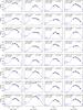 |
Fig. D.1 Far-IR SED fits of the Herschel stacked flux densities with Draine & Li (2007) templates. Each panel refers to a bin of the z–Mstar–SFR grid. The average value of redshift, stellar mass and SFR for galaxies belonging to each bin is printed in each panel. |
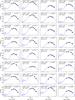 |
Fig. D.1 continued. |
 |
Fig. D.1 continued. |
 |
Fig. D.1 continued. |
Herschel is an ESA space observatory with science instruments provided by European-led Principal Investigator consortia and with important participation from NASA.
In deep 160, 250, 350 and 500 μm observations, rms values include confusion noise.
Publicly available at http://www.mpe.mpg.de/ir/Research/PEP/GOODSN_multiwave
Available at http://irsa.ipac.caltech.edu/data/COSMOS/tables/photometry/
Conversion factors to a Chabrier IMF are given in Sect. 3.6.
The statistics given in this section refers to the sample in the redshift and stellar mass range of interest and in the area over which the analysis is carried out (see Sect. 3.3).
This fraction refers to the sample over which the analysis is performed (see below and Sect. 3.5).
We use the Béthermin et al. (2010) libraries available at http://www.ias.u-psud.fr/irgalaxies/downloads.php
We verified that the trends presented in this analysis are independent of the chosen threshold.
Gas metallicities were measured from emission line ratios following Nagao et al. (2006) and Maiolino et al. (2008), i.e., from the [N iI]/Hα ratio and/or from the R23 = ([O iI]+[O iII])/Hβ quantity.
The term “integrated” refers to the measured power law relation between the gas mass and the SFR (see Sect. 5.1).
The fraction of stars which goes back into the ISM is ~30% for a Salpeter IMF (Treu et al. 2010).
We used the best-fit relation between FIR and CO luminosities in their Fig. 2 and the conversions given in their Table 1 to convert to SFR and Mgas, respectively.
Acknowledgments
P.S. thanks N. Scoville for interesting and useful discussions and A. Marconi and G. Risaliti for helping with fitting routines and statistical issues. This work was supported by grant ASI I/005/11/0. PACS has been developed by a consortium of institutes led by MPE (Germany) and including UVIE (Austria); KU Leuven, CSL, IMEC (Belgium); CEA, LAM (France); MPIA (Germany); INAF-IFSI/ OAA/OAP/OAT, LENS, SISSA (Italy); IAC (Spain). This development has been supported by the funding agencies BMVIT (Austria), ESA-PRODEX (Belgium), CEA/CNES (France), DLR (Germany), ASI/INAF (Italy), and CICYT/MCYT (Spain). SPIRE has been developed by a consortium of institutes led by Cardiff University (UK) and including University of Lethbridge (Canada), NAOC (China), CEA, LAM (France), IFSI, University of Padua (Italy), IAC (Spain), Stockholm Observatory (Sweden), Imperial College London, RAL, UCL-MSSL, UKATC, University of Sussex (UK), Caltech, JPL, NHSC, University of Colorado (USA). This development has been supported by national funding agencies: CSA (Canada); NAOC (China); CEA, CNES, CNRS (France); ASI (Italy); MCINN (Spain); SNSB (Sweden); STFC, UKSA (UK); and NASA (USA).
References
- de Prieto, C., Lambert, D. L., & Asplund, M. 2001, ApJ, 556, L63 [NASA ADS] [CrossRef] [Google Scholar]
- Andrews, B. H., & Martini, P. 2013, ApJ, 765, 140 [NASA ADS] [CrossRef] [Google Scholar]
- Asplund, M., Grevesse, N., Sauval, A. J., & Scott, P. 2009, ARA&A, 47, 481 [NASA ADS] [CrossRef] [Google Scholar]
- Bauermeister, A., Blitz, L., & Ma, C.-P. 2010, ApJ, 717, 323 [NASA ADS] [CrossRef] [Google Scholar]
- Belli, S., Jones, T., Ellis, R. S., & Richard, J. 2013, ApJ, 772, 141 [NASA ADS] [CrossRef] [Google Scholar]
- Berta, S., Magnelli, B., Lutz, D., et al. 2010, A&A, 518, L30 [NASA ADS] [CrossRef] [EDP Sciences] [Google Scholar]
- Berta, S., Magnelli, B., Nordon, R., et al. 2011, A&A, 532, A49 [NASA ADS] [CrossRef] [EDP Sciences] [Google Scholar]
- Berta, S., Lutz, D., Santini, P., et al. 2013, A&A, 551, A100 [NASA ADS] [CrossRef] [EDP Sciences] [Google Scholar]
- Béthermin, M., Dole, H., Beelen, A., & Aussel, H. 2010, A&A, 512, A78 [NASA ADS] [CrossRef] [EDP Sciences] [Google Scholar]
- Béthermin, M., Le Floc’h, E., Ilbert, O., et al. 2012, A&A, 542, A58 [NASA ADS] [CrossRef] [EDP Sciences] [Google Scholar]
- Bianchi, S. 2013, A&A, 552, A89 [NASA ADS] [CrossRef] [EDP Sciences] [Google Scholar]
- Bigiel, F., Leroy, A., Walter, F., et al. 2008, AJ, 136, 2846 [NASA ADS] [CrossRef] [Google Scholar]
- Bolatto, A. D., Wolfire, M., & Leroy, A. K. 2013, ARA&A, 51, 207 [Google Scholar]
- Bothwell, M. S., Maiolino, R., Kennicutt, R., et al. 2013, MNRAS, 433, 1425 [NASA ADS] [CrossRef] [Google Scholar]
- Bourne, N., Maddox, S. J., Dunne, L., et al. 2012, MNRAS, 421, 3027 [NASA ADS] [CrossRef] [Google Scholar]
- Brammer, G. B., van Dokkum, P. G., & Coppi, P. 2008, ApJ, 686, 1503 [NASA ADS] [CrossRef] [Google Scholar]
- Brinchmann, J., Charlot, S., White, S. D. M., et al. 2004, MNRAS, 351, 1151 [NASA ADS] [CrossRef] [Google Scholar]
- Bruzual, G., & Charlot, S. 2003, MNRAS, 344, 1000 [NASA ADS] [CrossRef] [Google Scholar]
- Buat, V., Noll, S., Burgarella, D., et al. 2012, A&A, 545, A141 [NASA ADS] [CrossRef] [EDP Sciences] [Google Scholar]
- Calura, F., Pipino, A., & Matteucci, F. 2008, A&A, 479, 669 [NASA ADS] [CrossRef] [EDP Sciences] [Google Scholar]
- Calzetti, D., Armus, L., Bohlin, R. C., et al. 2000, ApJ, 533, 682 [NASA ADS] [CrossRef] [Google Scholar]
- Capak, P., Aussel, H., Ajiki, M., et al. 2007, ApJS, 172, 99 [NASA ADS] [CrossRef] [Google Scholar]
- Chen, B., Dai, X., Kochanek, C. S., & Chartas, G. 2013, ApJ, submitted [arXiv:1306.0008] [Google Scholar]
- Conselice, C. J., Mortlock, A., Bluck, A. F. L., Grützbauch, R., & Duncan, K. 2013, MNRAS, 430, 1051 [NASA ADS] [CrossRef] [Google Scholar]
- Corbelli, E., Bianchi, S., Cortese, L., et al. 2012, A&A, 542, A32 [NASA ADS] [CrossRef] [EDP Sciences] [Google Scholar]
- Cortese, L., Ciesla, L., Boselli, A., et al. 2012, A&A, 540, A52 [NASA ADS] [CrossRef] [EDP Sciences] [Google Scholar]
- Cowie, L. L., Songaila, A., Hu, E. M., & Cohen, J. G. 1996, AJ, 112, 839 [Google Scholar]
- Cresci, G., Mannucci, F., Sommariva, V., et al. 2012, MNRAS, 421, 262 [NASA ADS] [Google Scholar]
- Daddi, E., Cimatti, A., Renzini, A., et al. 2004, ApJ, 617, 746 [NASA ADS] [CrossRef] [Google Scholar]
- Daddi, E., Elbaz, D., Walter, F., et al. 2010, ApJ, 714, L118 [Google Scholar]
- Dale, D. A., & Helou, G. 2002, ApJ, 576, 159 [NASA ADS] [CrossRef] [Google Scholar]
- Dale, D. A., Aniano, G., Engelbracht, C. W., et al. 2012, ApJ, 745, 95 [NASA ADS] [CrossRef] [Google Scholar]
- Davé, R. 2008, MNRAS, 385, 147 [NASA ADS] [CrossRef] [Google Scholar]
- Davé, R., Finlator, K., & Oppenheimer, B. D. 2011, MNRAS, 416, 1354 [NASA ADS] [CrossRef] [Google Scholar]
- Davé, R., Finlator, K., & Oppenheimer, B. D. 2012, MNRAS, 421, 98 [NASA ADS] [CrossRef] [Google Scholar]
- De Cia, A., Ledoux, C., Savaglio, S., Schady, P., & Vreeswijk, P. M. 2013, A&A, 560, A88 [NASA ADS] [CrossRef] [EDP Sciences] [Google Scholar]
- Donley, J. L., Koekemoer, A. M., Brusa, M., et al. 2012, ApJ, 748, 142 [NASA ADS] [CrossRef] [Google Scholar]
- Draine, B. T., & Lee, H. M. 1984, ApJ, 285, 89 [Google Scholar]
- Draine, B. T., & Li, A. 2007, ApJ, 657, 810 [NASA ADS] [CrossRef] [Google Scholar]
- Draine, B. T., Dale, D. A., Bendo, G., et al. 2007, ApJ, 663, 866 [NASA ADS] [CrossRef] [Google Scholar]
- Dunne, L., Gomez, H. L., da Cunha, E., et al. 2011, MNRAS, 417, 1510 [NASA ADS] [CrossRef] [Google Scholar]
- Eales, S. A., & Edmunds, M. G. 1996, MNRAS, 280, 1167 [NASA ADS] [CrossRef] [Google Scholar]
- Eales, S. A., Smith, M. W. L., Wilson, C. D., et al. 2010, A&A, 518, L62 [NASA ADS] [CrossRef] [EDP Sciences] [Google Scholar]
- Elbaz, D., Daddi, E., Le Borgne, D., et al. 2007, A&A, 468, 33 [NASA ADS] [CrossRef] [EDP Sciences] [Google Scholar]
- Elbaz, D., Dickinson, M., Hwang, H. S., et al. 2011, A&A, 533, A119 [NASA ADS] [CrossRef] [EDP Sciences] [Google Scholar]
- Fioc, M., & Rocca-Volmerange, B. 1997, A&A, 326, 950 [NASA ADS] [Google Scholar]
- Fiore, F., Grazian, A., Santini, P., et al. 2008, ApJ, 672, 94 [NASA ADS] [CrossRef] [Google Scholar]
- Fontana, A., Salimbeni, S., Grazian, A., et al. 2006, A&A, 459, 745 [NASA ADS] [CrossRef] [EDP Sciences] [Google Scholar]
- Fontana, A., Santini, P., Grazian, A., et al. 2009, A&A, 501, 15 [NASA ADS] [CrossRef] [EDP Sciences] [Google Scholar]
- Fontanot, F., De Lucia, G., Monaco, P., Somerville, R. S., & Santini, P. 2009, MNRAS, 397, 1776 [NASA ADS] [CrossRef] [Google Scholar]
- Gallerani, S., Maiolino, R., Juarez, Y., et al. 2010, A&A, 523, A85 [NASA ADS] [CrossRef] [EDP Sciences] [Google Scholar]
- Galliano, F., Hony, S., Bernard, J.-P., et al. 2011, A&A, 536, A88 [NASA ADS] [CrossRef] [EDP Sciences] [Google Scholar]
- Genzel, R., Tacconi, L. J., Gracia-Carpio, J., et al. 2010, MNRAS, 407, 2091 [NASA ADS] [CrossRef] [Google Scholar]
- Grazian, A., Fontana, A., De Santis, C., et al. 2006, A&A, 449, 951 [NASA ADS] [CrossRef] [EDP Sciences] [Google Scholar]
- Griffin, M. J., Abergel, A., Abreu, A., et al. 2010, A&A, 518, L3 [Google Scholar]
- Henry, A., Martin, C. L., Finlator, K., & Dressler, A. 2013a, ApJ, 769, 148 [NASA ADS] [CrossRef] [Google Scholar]
- Henry, A., Scarlata, C., Domínguez, A., et al. 2013b, ApJ, 776, L27 [NASA ADS] [CrossRef] [Google Scholar]
- Ilbert, O., Capak, P., Salvato, M., et al. 2009, ApJ, 690, 1236 [NASA ADS] [CrossRef] [Google Scholar]
- James, A., Dunne, L., Eales, S., & Edmunds, M. G. 2002, MNRAS, 335, 753 [NASA ADS] [CrossRef] [Google Scholar]
- Karim, A., Schinnerer, E., Martínez-Sansigre, A., et al. 2011, ApJ, 730, 61 [NASA ADS] [CrossRef] [Google Scholar]
- Kennicutt, Jr., R. C. 1998, ApJ, 498, 541 [NASA ADS] [CrossRef] [Google Scholar]
- Lagos, C. D. P., Baugh, C. M., Lacey, C. G., et al. 2011, MNRAS, 418, 1649 [NASA ADS] [CrossRef] [Google Scholar]
- Lamastra, A., Menci, N., Fiore, F., & Santini, P. 2013a, A&A, 552, A44 [NASA ADS] [CrossRef] [EDP Sciences] [Google Scholar]
- Lamastra, A., Menci, N., Fiore, F., et al. 2013b, A&A, 559, A56 [NASA ADS] [CrossRef] [EDP Sciences] [Google Scholar]
- Lara-López, M. A., Cepa, J., Bongiovanni, A., et al. 2010, A&A, 521, L53 [NASA ADS] [CrossRef] [EDP Sciences] [Google Scholar]
- Le Floc’h, E., Aussel, H., Ilbert, O., et al. 2009, ApJ, 703, 222 [NASA ADS] [CrossRef] [Google Scholar]
- Leroy, A. K., Bolatto, A., Bot, C., et al. 2009, ApJ, 702, 352 [NASA ADS] [CrossRef] [Google Scholar]
- Leroy, A. K., Bolatto, A., Gordon, K., et al. 2011, ApJ, 737, 12 [NASA ADS] [CrossRef] [Google Scholar]
- Li, A., & Draine, B. T. 2001, ApJ, 554, 778 [Google Scholar]
- Lutz, D., Poglitsch, A., Altieri, B., et al. 2011, A&A, 532, A90 [NASA ADS] [CrossRef] [EDP Sciences] [Google Scholar]
- Magdis, G. E., Daddi, E., Elbaz, D., et al. 2011, ApJ, 740, L15 [Google Scholar]
- Magdis, G. E., Daddi, E., Béthermin, M., et al. 2012, ApJ, 760, 6 [NASA ADS] [CrossRef] [Google Scholar]
- Magnelli, B., Lutz, D., Santini, P., et al. 2012a, A&A, 539, A155 [NASA ADS] [CrossRef] [EDP Sciences] [Google Scholar]
- Magnelli, B., Saintonge, A., Lutz, D., et al. 2012b, A&A, 548, A22 [NASA ADS] [CrossRef] [EDP Sciences] [Google Scholar]
- Magnelli, B., Lutz, D., Saintonge, A., et al. 2014, A&A, 561, A86 [NASA ADS] [CrossRef] [EDP Sciences] [Google Scholar]
- Maiolino, R., Nagao, T., Grazian, A., et al. 2008, A&A, 488, 463 [NASA ADS] [CrossRef] [EDP Sciences] [Google Scholar]
- Mannucci, F., Cresci, G., Maiolino, R., Marconi, A., & Gnerucci, A. 2010, MNRAS, 408, 2115 [NASA ADS] [CrossRef] [Google Scholar]
- Mannucci, F., Salvaterra, R., & Campisi, M. A. 2011, MNRAS, 414, 1263 [NASA ADS] [CrossRef] [Google Scholar]
- McCracken, H. J., Capak, P., Salvato, M., et al. 2010, ApJ, 708, 202 [NASA ADS] [CrossRef] [Google Scholar]
- Menci, N., Fiore, F., Puccetti, S., & Cavaliere, A. 2008, ApJ, 686, 219 [NASA ADS] [CrossRef] [Google Scholar]
- Mitchell, P. D., Lacey, C. G., Baugh, C. M., & Cole, S. 2013, MNRAS, 435, 87 [NASA ADS] [CrossRef] [Google Scholar]
- Nagao, T., Maiolino, R., & Marconi, A. 2006, A&A, 459, 85 [NASA ADS] [CrossRef] [EDP Sciences] [Google Scholar]
- Nakajima, K., Ouchi, M., Shimasaku, K., et al. 2012, ApJ, 745, 12 [NASA ADS] [CrossRef] [Google Scholar]
- Noeske, K. G., Weiner, B. J., Faber, S. M., et al. 2007, ApJ, 660, L43 [Google Scholar]
- Nordon, R., Lutz, D., Genzel, R., et al. 2012, ApJ, 745, 182 [NASA ADS] [CrossRef] [Google Scholar]
- Obreschkow, D., & Rawlings, S. 2009, ApJ, 696, L129 [NASA ADS] [CrossRef] [Google Scholar]
- Oliver, S. J., Bock, J., Altieri, B., et al. 2012, MNRAS, 424, 1614 [NASA ADS] [CrossRef] [EDP Sciences] [Google Scholar]
- Omukai, K., Tsuribe, T., Schneider, R., & Ferrara, A. 2005, ApJ, 626, 627 [NASA ADS] [CrossRef] [Google Scholar]
- Peng, Y.-J., Lilly, S. J., Kovač, K., et al. 2010, ApJ, 721, 193 [NASA ADS] [CrossRef] [Google Scholar]
- Pilbratt, G. L., Riedinger, J. R., Passvogel, T., et al. 2010, A&A, 518, L1 [CrossRef] [EDP Sciences] [Google Scholar]
- Poglitsch, A., Waelkens, C., Geis, N., et al. 2010, A&A, 518, L2 [NASA ADS] [CrossRef] [EDP Sciences] [Google Scholar]
- Popping, G., Somerville, R. S., & Trager, S. C. 2013, MNRAS, submitted [arXiv:1308.6764] [Google Scholar]
- Rémy-Ruyer, A., Madden, S. C., Galliano, F., et al. 2013, A&A, 557, A95 [NASA ADS] [CrossRef] [EDP Sciences] [Google Scholar]
- Rodighiero, G., Cimatti, A., Gruppioni, C., et al. 2010, A&A, 518, L25 [NASA ADS] [CrossRef] [EDP Sciences] [Google Scholar]
- Rodighiero, G., Daddi, E., Baronchelli, I., et al. 2011, ApJ, 739, L40 [NASA ADS] [CrossRef] [Google Scholar]
- Rosario, D. J., Santini, P., Lutz, D., et al. 2012, A&A, 545, A45 [NASA ADS] [CrossRef] [EDP Sciences] [Google Scholar]
- Roseboom, I. G., Oliver, S. J., Kunz, M., et al. 2010, MNRAS, 409, 48 [NASA ADS] [CrossRef] [Google Scholar]
- Roseboom, I. G., Ivison, R. J., Greve, T. R., et al. 2012, MNRAS, 419, 2758 [NASA ADS] [CrossRef] [Google Scholar]
- Saintonge, A., Tacconi, L. J., Fabello, S., et al. 2012, ApJ, 758, 73 [Google Scholar]
- Saintonge, A., Lutz, D., Genzel, R., et al. 2013, ApJ, 778, 2 [NASA ADS] [CrossRef] [Google Scholar]
- Sanders, D. B., Salvato, M., Aussel, H., et al. 2007, ApJS, 172, 86 [Google Scholar]
- Sandstrom, K. M., Leroy, A. K., Walter, F., et al. 2013, ApJ, 777, 5 [NASA ADS] [CrossRef] [Google Scholar]
- Santini, P., Fontana, A., Grazian, A., et al. 2009, A&A, 504, 751 [NASA ADS] [CrossRef] [EDP Sciences] [Google Scholar]
- Santini, P., Maiolino, R., Magnelli, B., et al. 2010, A&A, 518, L154 [NASA ADS] [CrossRef] [EDP Sciences] [Google Scholar]
- Santini, P., Fontana, A., Grazian, A., et al. 2012a, A&A, 538, A33 [NASA ADS] [CrossRef] [EDP Sciences] [Google Scholar]
- Santini, P., Rosario, D. J., Shao, L., et al. 2012b, A&A, 540, A109 [NASA ADS] [CrossRef] [EDP Sciences] [Google Scholar]
- Sargent, M. T., Béthermin, M., Daddi, E., & Elbaz, D. 2012, ApJ, 747, L31 [NASA ADS] [CrossRef] [Google Scholar]
- Sargent, M. T., Daddi, E., Béthermin, M., et al. 2013, ApJ, submitted [arXiv:1303.4392] [Google Scholar]
- Schmidt, M. 1959, ApJ, 129, 243 [NASA ADS] [CrossRef] [Google Scholar]
- Scoville, N. Z. 2012, Proceedings of the XXIII Canary Islands Winter School of Astrophysics: Secular Evolution of Galaxies (Cambridge University Press) [arXiv:1210.6990] [Google Scholar]
- Shao, L., Lutz, D., Nordon, R., et al. 2010, A&A, 518, L26 [NASA ADS] [CrossRef] [EDP Sciences] [Google Scholar]
- Silva, L., Granato, G. L., Bressan, A., & Danese, L. 1998, ApJ, 509, 103 [NASA ADS] [CrossRef] [Google Scholar]
- Smith, D. J. B., Dunne, L., da Cunha, E., et al. 2012, MNRAS, 427, 703 [NASA ADS] [CrossRef] [Google Scholar]
- Symeonidis, M., Vaccari, M., Berta, S., et al. 2013, MNRAS, 431, 2317 [NASA ADS] [CrossRef] [Google Scholar]
- Tacconi, L. J., Genzel, R., Neri, R., et al. 2010, Nature, 463, 781 [Google Scholar]
- Tacconi, L. J., Neri, R., Genzel, R., et al. 2013, ApJ, 768, 74 [Google Scholar]
- Treu, T., Auger, M. W., Koopmans, L. V. E., et al. 2010, ApJ, 709, 1195 [NASA ADS] [CrossRef] [Google Scholar]
- Weingartner, J. C., & Draine, B. T. 2001, ApJ, 548, 296 [NASA ADS] [CrossRef] [Google Scholar]
- Whitaker, K. E., van Dokkum, P. G., Brammer, G., & Franx, M. 2012, ApJ, 754, L29 [NASA ADS] [CrossRef] [Google Scholar]
- Wuyts, S., Förster Schreiber, N. M., Lutz, D., et al. 2011a, ApJ, 738, 106 [NASA ADS] [CrossRef] [Google Scholar]
- Wuyts, S., Förster Schreiber, N. M., van der Wel, A., et al. 2011b, ApJ, 742, 96 [NASA ADS] [CrossRef] [Google Scholar]
- Yates, R. M., Kauffmann, G., & Guo, Q. 2012, MNRAS, 422, 215 [NASA ADS] [CrossRef] [Google Scholar]
- Zafar, T., & Watson, D. 2013, A&A, 560, A26 [NASA ADS] [CrossRef] [EDP Sciences] [Google Scholar]
- Zahid, H. J., Dima, G. I., Kewley, L. J., Erb, D. K., & Davé, R. 2012, ApJ, 757, 54 [Google Scholar]
All Tables
Number of sources (upper number in each cell) and average dust mass (lower number in each cell) in each z–Mstar–SFR bin.
All Figures
|
Fig. 1 Example of the fits done to estimate the dust mass. Black symbols show stacked fluxes in the bin of the z–Mstar–SFR grid with z = [0.6,1), log Mstar [M⊙] = [10.75,11) and log SFR [M⊙/yr] = [1.4,1.6) The blue line shows the best-fit template from the library of Draine & Li (2007). For a comparison, the green and red curves show the fits with the GRASIL model and with a single-temperature modified blackbody (the latter not fitted to the shortest wavelength flux density), respectively. The dust mass inferred with the three libraries is indicated in the bottom right corner. The three libraries differ in the resulting dust masses by a roughly constant offset, but yield the same trends. |
| In the text | |
|
Fig. 2 SFR vs. dust mass in different redshift ranges. Galaxies are colour coded according to their stellar mass, as shown by the colour bar. The dashed lines corresponds to the integrated Schmidt-Kennicutt law fitted by Daddi et al. (2010), under the assumption of Solar metallicity (see text) and converted to a Salpeter IMF. |
| In the text | |
|
Fig. 3 Dust mass vs. stellar mass in different redshift ranges. Symbols are colour coded according to their SFR, as shown by the colour bar. At each Mstar, black open circles mark the bin which lies closest to the MS (in each Mstar interval), and in every case within 0.3 dex from it. The correlations between Mdust and Mstar are rather flat when the data points are separated by means of their SFR. The dashed lines correspond to an amount of dust equal to the maximum metal mass |
| In the text | |
|
Fig. 4 Average dust mass values, as indicated by the colour according to the colour bar, for bins of different SFR and Mstar in different redshift intervals and at all redshifts (upper right panel). Dashed lines represent MS relations of star-forming galaxies as taken from the literature; the local MS is from Peng et al. (2010) (computed using Brinchmann et al. 2004 data), rescaled to a Salpeter IMF, while the relations at higher redshifts are from Santini et al. (2009). Dotted lines represent the ± 1σ (=0.3 dex) scatter of the MS relation. |
| In the text | |
|
Fig. 5 Dust mass vs. stellar mass in panels of different SFR. The symbol colour indicates the mean redshift of each bin, as coded by the colour bar. No evolution with redshift is observed within uncertainties at a given Mstarand SFR. |
| In the text | |
|
Fig. 6 Left panel: relation between SFR and gas mass. The colour code indicates different redshift intervals, as shown by the legend in the upper left corner. The black boxes mark bins that lie in the starburst region according to Rodighiero et al. (2011). The solid thick black line is the power law fit to all data, and the best-fit relation is reported in the lower right corner. The dashed and dotted grey lines show the integrated Schmidt-Kennicutt relations fitted by Daddi et al. (2010) and Genzel et al. (2010), respectively, on normal star-forming galaxies (lower curves) and on local ULIRGs and z ~ 2 SMGs (upper curves). Curves from the literature are converted to a Salpeter IMF. Magenta dashed-dotted lines indicate constant star formation efficiencies (i.e., constant depletion times) of 1 (lower curve) and 10 (upper curve) Gyr-1. Right panels: relation between SFR and gas mass in different redshift bins, indicated in the upper left corner of each panel. Symbol styles and colours are as in the left panel. The coloured solid curves are the power law fits to the data, and the numbers in the lower right corner indicate the best-fit slope (upper) and intersection at log Mgas [M⊙] = 10 (lower) (see Eq. (7)). The dashed-triple dotted lines show the best-fit relation given in Eq. (8) calculated at the median redshift in each panel. |
| In the text | |
|
Fig. 7 Redshift evolution of the star formation efficiency (SFE, or inverse of the depletion time). Different colours refer to different SFRs, as shown by the colour bar. Black boxes are as in Fig. 6. |
| In the text | |
|
Fig. 8 Gas fraction vs. stellar mass in panels of different average SFR. The colour of the symbols reflects the mean redshift of each bin, as indicated by the colour bar. No evolution with redshift is observed, within uncertainties, at given SFR and Mstar. Grey dashed curves are the best-fits to the data assuming the functional shape in Eq. (9). Best-fit parameters for each SFR interval are summarized in Table 1. |
| In the text | |
|
Fig. 9 Average gas fractions, as indicated by the upper colour bar, in bins of Mstar and SFR. |
| In the text | |
|
Fig. 10 Parameterization of the gas fraction as a function of stellar mass at all redshifts in different SFR intervals, using the functional shape given in Eq. (9) (see text). Curves of different colours refer to different SFR bins, as shown by the colour bar. |
| In the text | |
|
Fig. 11 Representation of the 3D fundamental fgas–Mstar–SFR relation. The colour code indicates the average SFR of each bin. The best-fit relations shown in Fig. 8 are overplotted. |
| In the text | |
|
Fig. 12 Left: gas fraction vs. Mstar at different redshifts (in different colours according to the legend) for main sequence (MS) galaxies. Right: gas fraction vs. redshift at different Mstar (in different colours according to the legend) for MS galaxies. Curves are obtained by interpolating the fgas parameterizations reported in Fig. 10 and Table 1 and the MS relations (see text for details) at Mstar above the minimum sampled Mstar common to all SFR bins. Mean uncertainties on gas fraction associated to MS galaxies in each redshift (left) or stellar mass (right) bin are plotted. |
| In the text | |
|
Fig. 13 Predicted evolution of the gas fraction according to the semi-analytical model of Menci et al. (2008). The five filled contours indicate the fraction of galaxies having a given fgas at a fixed Mstar (left panels) and redshift (right panels). The trends for MS galaxies extrapolated from our observations (shown in Fig. 12) are overplotted. |
| In the text | |
|
Fig. B.1 Left: comparison between the 24 μm-based SFR used in the analysis (x-axis) and the SFR measured by fitting the average FIR stacked flux densities for each bin of the grid (y-axis). The colour code indicates the mean stellar mass in each bin. Right: same as the left panel, but FIR-based SFR are compared to the SFR measured by means of a “ladder” approach (see text). |
| In the text | |
|
Fig. C.1 Distribution of mock SFR and Mdust in input (left panel) and output (right panel) of the simulation described in text. The measure of the SFR and Mdust does not introduce a correlation in an initially uncorrelated distribution. The value of the Pearson coefficient is printed in both cases. |
| In the text | |
|
Fig. D.1 Far-IR SED fits of the Herschel stacked flux densities with Draine & Li (2007) templates. Each panel refers to a bin of the z–Mstar–SFR grid. The average value of redshift, stellar mass and SFR for galaxies belonging to each bin is printed in each panel. |
| In the text | |
|
Fig. D.1 continued. |
| In the text | |
|
Fig. D.1 continued. |
| In the text | |
|
Fig. D.1 continued. |
| In the text | |
Current usage metrics show cumulative count of Article Views (full-text article views including HTML views, PDF and ePub downloads, according to the available data) and Abstracts Views on Vision4Press platform.
Data correspond to usage on the plateform after 2015. The current usage metrics is available 48-96 hours after online publication and is updated daily on week days.
Initial download of the metrics may take a while.