| Issue |
A&A
Volume 556, August 2013
|
|
|---|---|---|
| Article Number | A136 | |
| Number of page(s) | 27 | |
| Section | Extragalactic astronomy | |
| DOI | https://doi.org/10.1051/0004-6361/201219998 | |
| Published online | 08 August 2013 | |
Near-infrared imaging spectroscopy of the inner few arcseconds of NGC 4151 with OSIRIS at Keck⋆
1
Physikalisches Institut, Universität zu Köln,
Zülpicher Strasse 77,
50937
Cologne,
Germany
e-mail:
This email address is being protected from spambots. You need JavaScript enabled to view it.
2
Deutsches SOFIA Institut, Universität Stuttgart,
Pfaffenwaldring 29,
70569
Stuttgart,
Germany
3
Division of Astronomy, University of California,
Los Angeles, CA
90095-1562,
USA
4
University of Rochester, Laboratory for Laser Energetics,
PO Box 278871,
Rochester, NY
14627-8871,
USA
5
Exoplanets and Stellar Astrophysics Laboratory,
Code 667, NASA Goddard Space Flight
Center, Greenbelt,
MD
20771,
USA
6
Landessternwarte, Zentrum fr Astronomie der Universität
Heidelberg, Königstuhl
12, 69117
Heidelberg,
Germany
7
Dunlap Institute for Astronomy & Astrophysics,
50 St. George
Street, Toronto,
ON, M5S 3H4, Canada
Received:
12
July
2012
Accepted:
18
March
2013
Abstract
We present H- and K-band data from the inner arcsecond of the Seyfert 1.5 galaxy NGC 4151 obtained with the adaptive-optics-assisted near-infrared-imaging field spectrograph OSIRIS at the Keck Observatory. The angular resolution is about a few parsecs on-site and thus competes easily with optical images taken previously with the Hubble Space Telescope. We present the morphology and dynamics of most species detected but focus on the morphology and dynamics of the narrow line region (as traced by emission of [FeII]λ1.644 μm), the interplay between plasma ejected from the nucleus (as traced by 21 cm continuum radio data) and hot H2 gas and characterize the detected nuclear HeIλ2.058 μm absorption feature as a narrow absorption line (NAL) phenomenon. The emission from the narrow line region (NLR) as traced by [FeII] reveals a biconical morphology and we compare the measured dynamics in the [FeII] emission line with models that propose acceleration of gas in the NLR and simple ejection of gas into the NLR. In the inner 2.5 arcsec the acceleration model reveals a better fit to our data than the ejection model. We also see evidence that the jet very locally enhances emission in [FeII] at certain positions in our field-of-view such that we were able to distinct the kinematics of these clouds from clouds generally accelerated in the NLR. Further, the radio jet is aligned with the bicone surface rather than the bicone axis such that we assume that the jet is not the dominant mechanism responsible for driving the kinematics of clouds in the NLR. The hot H2 gas is thermal with a temperature of about 1700 K. We observe a remarkable correlation between individual H2 clouds at systemic velocity with the 21 cm continuum radio jet. We propose that the radio jet is at least partially embedded in the galactic disk of NGC 4151 such that deviations from a linear radio structure are invoked by interactions of jet plasma with H2 clouds that are moving into the path of the jet because of rotation of the galactic disk of NGC 4151. Additionally, we observe a correlation of the jet as traced by the radio data, with gas as traced in Brγ and H2, at velocities between systemic and ±200 km s-1 at several locations along the path of the jet. The HeIλ2.058 μm line in NGC 4151 appears in emission with a blueshifted absorption component from an outflow. The emission (absorption) component has a velocity offset of 10 km s-1 (−280 km s-1) with a Gaussian (Lorentzian) full-width (half-width) at half maximum of 160 km s-1 (440 km s-1). The absorption component remains spatially unresolved and its kinematic measures differ from that of UV resonance absorption lines. From the amount of absorption we derive a lower limit of the HeI 21S column density of 1 × 1014 cm-2 with a covering factor along the line-of-sight of Clos ≃ 0.1.
Key words: galaxies: active / galaxies: Seyfert / galaxies: individual: NGC 4151
Figures 20–24 and Appendices are available in electronic form at http://www.aanda.org
© ESO, 2013
1. Introduction
NGC 4151 is a Seyfert 1.5 galaxy (Véron-Cetty & Véron 2006) originally cataloged by Seyfert (1943). Due to its proximity of about 13 Mpc it is an ideal testbed for the physics of active galactic nuclei (AGN) and therefore one of the most intensively studied Seyfert galaxies. In the AGN model proposed by Antonucci (1993) a supermassive black hole (SMBH) is surrounded by a dusty molecular torus. This torus is assumed to collimate the ionizing radiation field from the accretion disk that surrounds the SMBH. Seyfert galaxies as a class of AGNs are distinguished according to the viewing angle of the observer onto the obscuring torus. One of the most important topics in AGN research has been the search for the obscuring torus (for NGC 4151 see e.g. Pott et al. 2010), although the torus model has evolved significantly in the last decade (e.g. Elvis 2000). This torus is usually held responsible for the sometimes spectacular biconical emission morphologies of the narrow line region (NLR) (see e.g. Tadhunter & Tsvetanov 1989). In NGC 4151 emission of highly ionized species such as [OIII]λ501nm reveal an outflow into a bicone with a projected opening angle of 75° along a position angle (PA) of 60° (e.g. Kaiser et al. 2000). Thompson (1995) showed, that most of the iron in the NLR is in the gaseous phase, and because the kinematics observed in [OIII] is similar to that observed in [FeII]λ1.257 μm and Paβλ1.282 μm (Knop et al. 1996), emission of [OIII] and [FeII] is most likely due to photoionization by the AGN. However, [FeII] emission line profiles appear broader than e.g. Paβ line profiles along the NLR such that additional mechanisms may be necessary to locally enhance emission of [FeII], like shocks in a wind from the AGN or a jet. A faint spatially resolved jet emerging from the nucleus has been observed by Mundell et al. (2003) and others. The jet extends several arcseconds at a PA of about 77° and is therefore misaligned with the NLR bicone axis by about 15°. However, the inclination of the jet with respect to the galactic plane of NGC 4151 is assumed to be low such that interactions of the jet with the interstellar medium in the galactic disk of NGC 4151 are likely to occur and, indeed, some correlation between the jet and [FeII]λ1.644 μm emission knots has been observed (Storchi-Bergmann et al. 2009). The dynamics within the NLR has been modeled by several authors (Crenshaw et al. 2000b; Das et al. 2005; Storchi-Bergmann et al. 2010) assuming acceleration in an outflow and simple ejection with no acceleration. But the dynamics of gas within the NLR maybe more complex. The mass outflow rate into each cone is about 100 times higher than the accretion rate (Storchi-Bergmann et al. 2010), which indicates that the origin of the outflowing gas is not the AGN but surrounding gas of the galaxy interstellar medium that is accelerated in a nuclear outflow. Additionally, the activity of the nucleus of NGC 4151 is also known to vary on timescales of months, and the velocities of the nuclear outflow (as observed in P-Cygni HeIλ388.8 nm and Balmer absorption) change on the same timescale (Hutchings et al. 2002). However, the dynamics and morphology of the NLR is still puzzling and the role of the radio jet is not fully understood (e.g. why does the radio jet show an S-like structure as reported by Mundell et al. 2003?). In the inner 250 parsec of the galactic disk of NGC 4151 a large reservoir of hot H2 gas is seen (e.g. Fernandez et al. 1999). This gas is in thermal equilibrium and is most likely heated by X-rays (Storchi-Bergmann et al. 2009) or by shocks from gas inflowing from larger distances (Mundell & Shone 1999; Mundell et al. 1999). This reservoir is usually considered responsible for feeding the AGN while the outflow into the NLR is considered as the feedback (Storchi-Bergmann et al. 2010), although the final feeding stage (at the sphere of influence) has not been observed yet.
In this paper we present data obtained during one of the first commissioning runs with the near-infrared imaging field spectrograph OSIRIS at the Keck observatory. Our observations have angular resolutions corresponding to a few parsecs on-site, such that we can address the questions mentioned above. Our integral field data are perfectly suited to derive the dynamics from within a truly two-dimensional field-of-view (FoV). Additionally, our near-infrared observations are less hampered by dust extinction and allow angular resolutions at the diffraction limit of the Keck telescope when using adaptive optics.
The paper is organized as follows: In Sect. 2 we summarize the instrumental setup and our observations. Section 3 briefly summarizes the data reduction methods. In Sect. 4 we discuss continuum emission. In Sect. 5 we present emission line morphologies of all prominent species, and we discuss their dynamics in Sect. 6. In Sect. 7 we describe the excitation mechanisms of H2 and calculate column densities of the ro-vib transitions of H2 and HeI. We conclude in Sect. 8 with a summary of our findings.
In this paper we use h0 = 75 km s-1/Mpc, implying linear distances of 64 pc/arcsec at a distance of 13.25 Mpc.
2. Observations
NGC 4151 was observed in 2005 February and May as one of the first commissioning targets for the OH Suppressing InfraRed Imaging Spectrograph (OSIRIS) at the W. M. Keck Observatory. OSIRIS is an integral field spectrograph (Larkin et al. 2006) for the near-infrared (z, J, H and K band) with a nominal spectral resolution of λ/Δλ = 3700 (corresponding to 5 Å or 60 km s-1) mounted on the Nasmyth platform of the Keck II telescope, which works with the Keck adaptive optics system (Wizinowich et al. 2000). The design of the instrument is based on concepts developed for the TIGER spectrograph (Bacon et al. 1995) and uses an infrared transmissive microlens array that samples a rectangular FoV of the adaptive optics focal plane. The selectable plate scales are 20, 35, 50, and 100 milli-arcsec (mas) per angular resolution element. Each microlens focuses the light into a pupil image that serves as input to the actual spectrograph which consists of a collimator (a three-mirror-anastigmat), a diffraction grating, a three-mirror camera, and a Hawaii II HgCdTe detector (with 2048 × 2048 pixel and 32 output channels). The readout noise of the detector is 13 e− per single read, and the detector is read in sampling-up-the-ramp mode. OSIRIS offers several near-infrared broad- and narrowband filters. The number of angular resolution elements, hence the size of the FoV, is filter dependent (see Appendix A). Additionally, OSIRIS is equipped with an imaging camera hosting a HAWAII I detector (1024 × 1024 pixel). The FoV of the camera is 20 arcsec and is offset by 20 arcsec from the center of the FoV of the spectrograph.
We performed spectroscopic H narrowband and K broadband adaptive optics (AO) assisted observations of the inner few arcseconds of the Seyfert 1.5 galaxy NGC 4151 (see Table 1 for details about the observations). The plate scales were 35 mas (in H band) and 50 mas (in K band) per angular resolution element corresponding to linear distances of 2.2 pc and 3.2 pc at the location of NGC 4151. The total on-source integration times were 8.3 min in H band and 50 min in K band. The AO system1 was operated in natural guide star (NGS) mode with the bright central AGN of NGC 4151 as point spread function (PSF) reference source. The AO correction rate during both nights was higher than 100 Hz and the measured full-width at half maximum (FWHM) of the AGN in K broadband after data reduction varied between 80 mas (at 2.3 micron) and 140 mas (at 2 micron) (the theoretical FWHM of the diffraction spike of the Keck telescope is approximately 60 mas in the K band). In K-broadband mode the FoV format is 3.20 × 0.95 arcsec and covers 64 × 19 field points. We observed using the classical AB pattern with a sky offset of 20 arcsec. Because the FoV in the K-broadband mode is extremely narrow, we observed NGC 4151 at different position angles (PA) keeping the AGN always centered to have a well-defined reference position for mosaicking. In H narrowband the FWHM is about 80 mas. The FoV format is 2.31 × 1.79 arcsec and covers 66 × 51 field points, and we used the same sky offset as in the K broadband. We observed the A0V stars HD 140729 and HD 105601 as tellurics.
Observation summary.
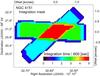 |
Fig. 1 Size of our FoV after mosaicking and total on-source integration time in the K band. |
3. Data reduction and integrated flux values
In this section we briefly summarize the various data reduction steps. We refer to appendix A for a more detailed discussion of the data reduction concept for OSIRIS commissioning data, about the OSIRIS data reduction pipeline (DRP) in general, and about details of the various data reduction steps involved.
The first data reduction step is the subtraction of the sky followed by a bad-pixel search and a one-dimensional interpolation of the bad pixels along the dispersion axis. Supplementary reduction steps to cope with detector artifacts such as time variable direct current (DC) biases in the 32 multiplexer readout channels or electronic ghosts followed. The next step was reconstructing the distribution of incident light on the microlens array from the recorded detector image in a process called rectification. In this process we used PSFs of each microlens on the detector, recorded during daytime. After rectification, the light in each reconstructed spectrum was assigned to a specific microlens. The spectra were then wavelength calibrated and interpolated onto a regular wavelength grid with a sampling close to the intrinsic sampling (2.5 Å in K broadband and 2.0 Å in H narrowband, corresponding roughly to 30 km s-1 and 35 km s-1 per spectral channel respectively). The spectra were rearranged according to their proper positions on the sky to a data cube with an α, a δ and a λ axis. Once the data cube was constructed, additional reduction steps, e.g., three-dimensional bad-pixel identification and interpolation, or correction for atmospheric differential refraction were applied.
From here, our K- and H-band observations were treated differently. For our K-broadband observations, the shift of the FoV with increasing wavelength in the data cube due to atmospheric differential refraction was determined to be less than 1/4 of an angular resolution element between 2.0 and 2.3 μm, and were not corrected. The spectra of the telluric standard stars were extracted from a 400 mas-wide circular aperture. The intrinsic Brγ absorption line at 2.166 μm in the extracted telluric spectrum (A0V star) was fitted with a Lorentzian, and the fit was subtracted from the spectrum. Then we divided the extracted spectrum by a blackbody (T = 9600 K) to correct for the intrinsic continuum emission of the telluric stars. In the NGC 4151 datacubes some spectra show residuals after division with the telluric spectrum due to an imbalanced sky subtraction, especially in wavelength regimes of low atmospheric transmission. We added appropriate biases to these spectra prior to division by the telluric spectrum to correct for this imbalance. The resulting five data cubes of NGC 4151 were finally rotated to a common PA, shifted to a common reference position, in our case the point-like AGN, and were averaged. We applied no telluric correction to our H-narrowband observations, since in this wavelength band A0V stars exhibit quite a few strong absorption lines from hydrogen and helium and the transmission of the atmosphere in this wavelength range is nearly constant and higher than 95%. However, we compared our telluric spectrum with an A0V spectrum from Pickles (1998) to check for instrument-specific transmission effects. Within the signal-to-noise ratio achieved in every spectrum, neither atmospheric nor instrumental transmission affect the result. Finally, the telluric standards were used to flux-calibrate our data by applying the Vega flux densities listed in Allen (2000).
We follow convention and refer to a spectrum corresponding to one spatial position in the data cube as a spaxel. The individual data elements of a spaxel are refered to as spexels. The integration mask of the mosaicked K-broadband data cube is presented in Fig. 1. In that figure the effective integration time for each spaxel is coded in color, which also provides an assessment about the relative signal-to-noise ratio (S/N) throughout the FoV. From the distribution of the colors one can also trace the contribution of individual data cubes to the x-shaped final mosaic. Maximum overlap occurs within the central 500 mas. The H-band integration map is not shown, since only one data cube was obtained. The designated coordinates in right ascension and declination are derived from the radio map presented in Mundell et al. (2003), where the authors identified the position of the bright AGN with component D of the radio jet. On-nucleus and off-nucleus K-band spectra are displayed in Fig. 2. Table 2 lists fluxes of all species detected in our H- and K-band data. Channel maps of the most prominent line emission/absorption features are presented in the appropriate sections below.
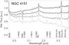 |
Fig. 2 K-band spectra of NGC 4151 extracted from circular apertures with a radius of 125 mas. From top to bottom: nucleus, region 160 mas southwest of the nucleus, region 160 mas north of the nucleus, and region 600 mas northwest of the nucleus. The spectra are normalized to unity at 2.245 μm and shifted by multiples of 0.15. Detected species are indicated. |
Flux values of detected species derived from integrating the whole field-of-view and from a circular aperture with a radius of 300 mas centered on the bright H2 region in the southeast.
4. Continuum emission
4.1. Shape and spectral profile
Pseudo H- and K-band images of the NGC 4151 nuclear region were created by collapsing the respective data cubes along their wavelength axes. They are displayed in Fig. 3. The K-band flux is FK = 2.6 × 10⁻¹⁴ W/m2 from our full aperture and FK = 3.95 × 10⁻¹⁵ W/m2 from a circular aperture with a radius of 100 mas centered on the fitted continuum peak between 1.965−2.381 μm.
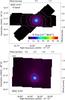 |
Fig. 3 K-band image (1.965−2.381 μm) (top) and H-band image (1.594−1.676 μm) (bottom) of NGC 4151 with corresponding continuum contours at (1%, 2%, 4%, K only), 8% ,16%, 32% and 64% of the maximum level. North is up and east to the left. |
In both wavelength bands the continuum contours are almost circular, in particular within the region of maximum overlap where the S/N peaks. The contours are extending the circular contours observed by Peletier et al. (1999) on larger scales. Small deviations from circularity are, however, notable in both bands. We also note discontinuities in the K-band continuum image along the lower rim of the horizontal stretch and close to the southeastern end of the tilted stretch. These features can be attributed to different seeing conditions prevailing during the observations of the five individual data cubes (see also Appendix B).
Figure 4 shows the flux density ratio around 2.35 and 2.09 μm extracted from continuum emission free of absorption and emission lines. The ratio is about 1.3 on the nucleus and drops to 0.8 at larger distances to the nucleus. Figure 4 also reveals that the flux density ratio contours (the white contours in Fig. 4 correspond to a flux density ratio of 0.9) deviate significantly from the almost circular shape of the K-band continuum contours in Fig. 3 (top) and are elliptical (even boxy). The effect of variable seeing conditions on the mosaicked datacube is also discussed in Appendix B and cannot be accounted for by the observed asymmetry. The spectra are redder along a long axis PA of −60° with an extent of approximately 15 pc and a long/short axis ratio of 1.5/1. Interestingly, this direction roughly complies with the direction of the H2-emitting bicone (as shown in Fig. 4 and described below).
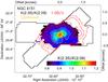 |
Fig. 4 Flux density ratio of emission- and absorption-line-free continuum emission around 2.35 and 2.09 μm. H2 (1-0S(1)) contours in red, flux ratio contour of 0.9 in white. Continuum contours (20% and 50% of the peak intensity) in yellow. North is up and east to the left. |
4.2. Spectral decomposition and stellar content
The continuum emission is composed of stellar and non-stellar contributions. The stellar contribution can be quantified using pronounced stellar absorption features like the CO absorption bandheads around 2.3 μm, while contributions from non-stellar continuum emission sources can only be quantified by evaluating the overall continuum slope over a wide wavelength range. Following Krabbe et al. (2000), we decomposed the continuum into stellar components and non-stellar components, e.g., emission of hot dust, AGN power-law emission, and free-free emission (see Appendix C for a detailed description of the decomposition algorithm). For every measured spectrum we subsequently generated a synthetic continuum spectrum, reddened it, and compared it with the measured spectrum in terms of minimizing the χ2 difference between the two.
Three effects complicate a proper decomposition of the continuum emission for every pixel in the FoV, the broadening of the PSF with wavelength, broad emission lines such as Brγ, and the limited wavelength coverage of our data. For instance, Riffel et al. (2009) decomposed the nuclear continuum spectrum of NGC 4151 using a wavelength coverage from 0.4 μm to 2.4 μm. Nevertheless, it is well possible to decompose the continuum emission into stellar and non-stellar contributions (on the basis of the depth of the CO absorption bandheads), and we constrain ourselves here to find the position of the nuclear star cluster. We did not attempt to decompose the non-stellar emission into its individual components.
Before decomposing we needed to estimate the dominating spectral type of the stellar continuum. Prominent features in the stellar continuum in the near-infrared are the CO absorption bandheads around 2.3 μm, the NaI absorption doublet around 2.208 μm, and the CaI triplet around 2.264 μm. The last two are either too weak to be identified in each individual spectrum or are strongly diluted by the non-stellar continuum. We summed all spectra from an annulus with an inner radius of 300 mas and an outer radius of 600 mas and applied our decomposition algorithm using all spectra from the Wallace and Hinkle stellar library (Wallace & Hinkle 1997). K and M supergiants match the total off-nuclear spectrum best, and we used the spectrum of HR8726, a K5Ib star, as stellar template (see Fig. 5).
The stellar and non-stellar continuum emission peaks coincide. At this position the stellar continuum emission drops to a very few percent (of the total continuum), and both peaks appear to be unresolved, although the stellar continuum emission can be traced further out, where it reveals the stellar disk of NGC 4151.
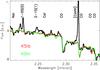 |
Fig. 5 Spectrum (black) extracted from an annuli with an inner radius of 300 mas and an outer radius of 600 mas. The artificial spectrum using the template stars HR8726/HR8694 is overplotted in red/green. |
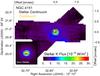 |
Fig. 6 Stellar flux derived from the spectral decomposition described in the text. The non-stellar continuum is not on the same flux scale. Corresponding continuum contours (20% and 50% of the peak intensity) are denoted in yellow. North is up and east to the left. |
5. Morphology of emission and absorption lines
NGC 4151 as a whole has been classified as a (R’)SAB(rs)ab barred spiral (Sérsic & Pastoriza 1965). The inclination and PA of the galactic disk have been determined from HI observations and optical observations to be i ≃ 23° with a PA of 22° (e.g. Davies 1973; Pedlar et al. 1992; Simkin 1975). The observed HI dynamics and the orientation of the spiral arms indicate that the galactic plane is closer to the observer at the southeast. There is an inner bar with a PA ≃ 130° deduced from brighter isophotes (Davies 1973; Simkin 1975; Pedlar et al. 1992). Mundell & Shone (1999) and Mundell et al. (1999) conducted HI observations that revealed an elliptical HI structure with a diameter of a very few arcminutes around the nucleus along a PA of about −60°, referred to as the oval. They concluded that the oval is a kinematically weak bar along which the authors detected inflow of gas to the nucleus, which may represent an early stage of the fueling process. Further inside at distances of a few arcseconds around the nucleus, Fernandez et al. (1999) observed emission of ro-vib transitions of H2. Observations made with the Hubble Space Telescope in the optical ([OIII]λ501 nm) revealed a biconical emission morphology of the NLR with an opening angle of approximately 30° at a PA of 60°, extending several arcseconds to either side of the nucleus (Evans et al. 1993; Hutchings et al. 1998; Kaiser et al. 2000). The orientation of the galactic disk and the bicone as they appear on the sky is shown in the next section in Fig. 17, where we discuss in detail the dynamics seen in individual emission lines. Finally, Mundell et al. (2003) observed the 21 cm continuum radio jet that emerges from the nucleus and extends several arcseconds from the nucleus with a PA of about 77°. The orientation of the line-of-nodes of the galactic disk, the bar, the radio jet, and the NLR bicone axis are shown in Fig. 7.
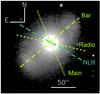 |
Fig. 7 K-band image of NGC 4151 taken from Knapen et al. (2003). The axes indicate the main kinematical axis (Main), the radio axis (Radio), the orientation of the bar (Bar) and the direction of the NLR bicone axis (NLR). |
5.1. Extraction
Flux maps were extracted with FLUXER, an analyzation and visualization tool for astronomical data cubes written in IDL. Since most line profiles deviate strongly from a Gaussian, we used the following method to extract flux maps: The continuum around an emission line was fitted with a parabola and subtracted from the spectrum. From the center of intensity position within the line profile all spexels with increasing/decreasing wavelength were summed as long as the spexel value in the continuum subtracted spectrum was positive. Prior to extracting the fluxes, we smooth each slice of the datacube with constant wavelength with a boxcar to increase the S/N ratio, if noted. Since the angular resolution therefore depends on the above smoothing process, we usually added continuum isophotes of 50% and 20% of the continuum peak flux at the wavelength of the emission line to our images. The wavelength dependence of our angular resolution can also be inferred from the continuum isophotes of Fig. 11, where no smoothing was applied.
5.2. Morphology
In the following we present and compare near-infrared emission line maps of e.g. Brγλ2.16 μm, ro-vib transitions of molecular hydrogen, [FeII]λ1.644 μm, [CaVIII]λ2.321 μm, [SiVI]λ1.963 μm, and HeIλ2.058 μm (the latter also appears in absorption in nuclear spectra).
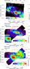 |
Fig. 8 Top: [FeII]λ1.644 μm emission, [OIII]λ501 nm emission contours taken from Kaiser et al. (2000) in yellow and 21 cm radio contours taken from Mundell et al. (2003) in white. Our naming scheme for the prominent [FeII] emitting regions (F1-3) and the 21 cm radio continuum knots (R2E, R1E, R1W, R2W) is indicated. Radio contours in levels of .5 and 1 mJy beam-1 only. Middle: Brγ emission map extracted from a running aperture of 3 × 3. [FeII] emission contours in red, 21 cm emission contours in yellow. Inset: The inset shows Brγ emission from the nuclear region on the same flux scale. The orange contours represent continuum isophotes (50% and 20% of the peak value) at the wavelength of Brγ. Bottom: integrated 1-0S(0-2) flux, [FeII]λ1.644 μm, and 21 cm radio data taken from Mundell et al. (2003). The H2 data were extracted the same way as the Brγ emission map. All figures: north is up and east to the left. Radio contours in levels of .5, 1, 2, and 4 mJy beam-1 with a beam size app. four times smaller than our angular sampling. |
5.2.1. Emission from within the NLR
We used emission of [FeII]λ1.644 μm (see Fig. 8, top) to trace the NLR. The emission arises from a biconical structure with a position angle of approximately 60° with a projected opening angle of 75°. The emission morphology appears to be clumpy and most of the emission is detected from the position of the continuum peak. There is a clumpy arc of [FeII] located approximately 1 arcsec to the northeast extending north (region F1 hereafter), a knot approximately 0.5 arcsec to the west (region F2), and another extended structure 0.75 arcsec to the southeast (region F3). Since [FeII] and [OIII] emission are both assumed to be due to photoionization by the AGN (Knop et al. 1996), we overplotted the contours of [OIII]λ501 nm taken from Kaiser et al. (2000) on our [FeII] flux map. The [OIII] emission appears to be clumpy as well, with emission from the same [FeII] regions as mentioned above, but also from beyond. The 21 cm continuum radio data taken from Mundell et al. (2003) are also overplotted in Fig. 8 (top). Their radio component D correlates with the position of the AGN, and our data are aligned such that the position of this radio component is identical with the position of the bright continuum peak that we assume to be the AGN. The radio emission extends linearly from the nucleus at a PA of 77°. In the case of NGC 4151 the radio jet is misaligned by 15° with the NLR’s major axis if deduced solely from [FeII] or [OIII] morphologies. Within our FoV we detect four bright radio knots (plus the bright radio knot at the position of the continuum peak), approximately 0.5 and 1.0 arcsec to the east (regions R1E and R2E) and 0.4 and 0.75 arcsec to the west (regions R1W and R2W) from the continuum peak. The knots closer to the nucleus (the inner knots, with index 1) appear to extend roughly linearly from the nucleus at a PA of app. 80°, while the knots at larger distances (outer knots with index 2) seem to deviate from this straight line to a PA of about 72°, causing the jet to appear S-shaped. The outer eastern radio knot (R2E) correlates well with the south end of the [FeII] arc (F1) and the inner western radio knot (R1W) correlates well with F2. Together with the above mentioned misalignment of the jet with the main axis of the NLR (based on the [FeII] and [OIII] morphologies), we conclude from these velocity-integrated flux maps that the excitation in the NLR maybe partially enhanced by the jet. We discuss the correlation of the radio jet with [FeII] emission at individual velocities in the next section. We did not observe enhanced [FeII] emission from the locations where deviations from the straight jet axis occur.
At the nucleus the Brγ emission line shows a prominent broad component (with a Gaussian FWHM of several thousand km s-1) with a narrow component at the top. In the following we discuss the narrow emission of Brγ only. The morphology of Brγ (Fig. 8, middle) appears to be less clumpy than [FeII] with smoothly distributed emission along the NLR. The emission peak in Brγ is located approximately 10 pc to the northwest at a PA of −50° of the continuum peak (see the inset in Fig. 8, middle). We detect Brγ emission knots at the locations of the [FeII] knots F2 and F3 (all to the west of the nucleus), but not at locations where the 21 cm radio continuum is prominent. However, Brγ isophotes seem to extend along a PA of about 70° and to locations where the inner radio knots are observed.
The HeI n = 21P − n = 21S at 2.0581 μm emission line in nuclear spectra is accompanied by a blueshifted optically thin absorption complex that is marginally resolved in the spectra presented by Riffel et al. (2006).
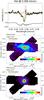 |
Fig. 9 HeIλ2.0581 μm line complex. Top: continuum-subtracted line complex of HeI extracted from a circular aperture with a radius of 400 mas centered on the nucleus; data are plotted in black, the fitted Lorentzian absorption and Gaussian emission components are plotted in red, total fit plotted in green. The continuum was fitted with a parabola using emission/absorption-free wavelength channels to the left and to the right of the line complex. Below the extracted line complex we plot the telluric spectrum around the HeI line complex. In this spectral regime the atmospheric transmission drops to about 75%, as indicated. Middle and bottom: HeI emission (middle) and absorption flux (bottom) derived from the three-component fit, as explained in the text. To increase the S/N we used a running aperture of 5 × 5 prior to extraction. Continuum isophotes are marked in yellow at the wavelength of HeI for 20% and 50% of the continuum peak intensity. North is up and east to the left. Radio contours in emission map in levels of .5, 1, 2, and 4 mJy beam-1 with a beam size about four times smaller than our angular sampling. |
The atmospheric transmission around that emission line highly depends on wavelength (see the telluric spectrum in Fig. 9, top). Hence, a proper telluric correction is critical and was performed as described in the data reduction section to ensure a smooth continuum around the line complex. Figure 9 (top) shows the continuum-subtracted spectrum around the HeI complex extracted from a circular aperture with a radius of 400 mas centered on the nucleus. To extract the flux and determine the amount of absorption, we fit a Gaussian emission component and two Lorentzian absorption components to the line complex. The results of our fits (flux, Gaussian and Lorentzian widths, equivalent widths, and column densities derived from the absorption component) are summarized in Table 3. The deeper absorption component is blueshifted by −280 km s-1 and the weaker by −1150 km s-1. However, we detect the absorption component with the larger velocity offset everywhere in our FoV, which indicates that this component is a residual in our data reduction.
Results of the fit to the nuclear HeIλ 2.0581 μm line complex.
Figure 9 (middle and bottom) shows the derived HeI morphology (integrated emission and absorption) deduced from our fits. The emission component extends into the direction of the NLR and is well comparable with the Brγ emission morphology with two exceptions: the HeI emission peaks at the position of the continuum peak, and we observe no significant HeI emission at F3, where [FeII] and Brγ are bright. The integrated absorption component peaks at the nucleus but remains unresolved (as indicated by a radial plot of the continuum and the integrated absorption flux in Fig. 10). The HeI absorption seems to be a local feature of the nucleus, occurring closer to it than the resolution limit of our observations (a few parsecs).
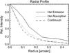 |
Fig. 10 Radial profiles of the HeIλ2.0581 μm emission and absorption and continuum flux at the position of the HeI line. |
5.2.2. Emission from beyond the NLR
In contrast to the morphologies of Brγ and HeI, which extend into the NLR, the H2 morphology is completely different and extends nearly perpendicular to the NLR, thus avoiding the NLR (see Fig. 8, bottom). The H2 emission is most pronounced along a PA of about −50° and is roughly aligned with the bar and the galaxy minor axis. In the northwestern region the H2 emission appears to be clumpy on scales of a few pc and reveals a shell-like structure. In the southeast the emission appears to be less clumpy. Toward the south of the inner shell-like structure in the northwest, at the edge of our field-of-view, the H2 emission increases such that the H2 emitting region is not fully sampled by our FoV. There is a remarkable correlation between parts of the H2 emission morphology and the 21 cm continuum radio jet. Deviations from the straight radio jet axis (drawn from the inner jet knots) occur exactly at the edges of bright H2 clouds (see especially the radio knot associated with the southern extension of the outer shell in the northwest). Following Wilson & Ulvestad (1982), we propose that the 21 cm radio is indeed arising from regions in space where H2 gas in the galactic disk is rotating clockwise (Mundell et al. 1995) into the path of the jet, giving rise to the remarkable interaction zones. The [FeII] emission does not originate from the same regions on the sky as the H2 emission, which is compatible with the assumption that emission from the NLR originates from regions exposed to the radiation field of the AGN where H2 molecules dissociate.
Although our FoV does not sample the full inner two arcseconds due to its X-shape, the H2 emission does not extend significantly beyond our FoV (see Storchi-Bergmann et al. 2009). It is possible that the pronounced H2 emission morphology represents another feeding stage of the HI bar observed by Mundell et al. (1999) but closer to the nucleus. These authors detected an oval distortion in the inner two arcminutes resembling a rotating, inclined HI ring or disk (see their Fig. 5), referred to as the oval. However, the velocity field of the oval differs significantly from a rotating, inclined disk because the isovelocity contours are elongated along the oval. Additionally, Mundell et al. (1999) detected bright HI regions close to the leading edges of the oval whose kinematics shows signature of a bar shock. From this they concluded that the oval is a kinematically weak bar. Subtracting a radial velocity field of purely circular rotation reveals that gas may stream along that bar at a PA of −60° toward the nucleus (Mundell & Shone 1999), which they interpreted as an early stage of the fueling process. The position angle of this bar is −60° and thus roughly coincides with the position angle drawn from the most prominent H2 regions. It is possible that the observed emission of H2 is at least enhanced by this inflow of gas to the central 200 parsecs. There is also a weak bridge of hot H2 gas between the two large gas reservoirs to the southeast and the northwest that runs through the nucleus.
5.2.3. Coronal emission lines
NGC 4151 is an archetypical Seyfert galaxy, and strong emission of coronal lines in [CaVIII] and [SiVI] is detected. The [CaVIII] emission profile is strongly affected by the CO3-1 absorption bandhead. The continuum emission was modeled with the spectral decomposition algorithm prior to extracting the [CaVIII] channel map. The emission line profiles of [CaVIII] and [SiVI] (see Fig. 12) are very similar, but show a very weak blueshifted hump compared to the much narrower 1-0S(1) line. Fitting two Gaussians to the coronal emission line reveals a broader component that is marginally blueshifted by one spectral channel (app. 35 km s-1). The FWHMs are 950 km s-1 of the broader and 230 km s-1 of the narrower component (not corrected for instrumental resolution). The considerable broadening of the blueshifted component may indicate that the [CaVIII] emission at least partially arises from a shock-excited region close to the nucleus (Prieto et al. 2005).
The morphology of the [CaVIII] and [SiVI] emission is shown in Fig. 11. Extended emission from both species is detected (at systemic velocity) from the NLR at distances of up to 50 pc from the nucleus. This may imply an energetic radiation field in the galactic plane of NGC 4151 that is possibly due to a clumpy obscurer of the nuclear radiation field. Emission of both species peaks close to the nucleus. However, a closer inspection of the dataset with 20 mas sampling (see inset in Fig. 11, top) reveals that e.g. the [CaVIII] peak is located approximately 6 parsecs to the west of the continuum peak and that both peaks are resolved. The peak in the [SiVI] emission map seems to be less pronounced than the [CaVIII] peak, but the performance of the AO is wavelength dependent, as indicated by the more extended continuum contours in the [SiVI] image that pretend different morphologies.
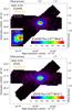 |
Fig. 11 [CaVIII] (top) and [SiVI] (bottom) emission morphology extracted from every spaxel. The yellow contours represent continuum isophotes at the wavelength of [CaVIII] for 20% and 50% of the continuum peak intensity. The inset (top figure) shows a [CaVIII] emission map derived from the data set with a sampling of 20 mas per pixel. North is up and east to the left. |
To test whether the two species are differently distributed, the [CaVIII] emission map was convolved with a Gaussian seeing disk such that the continuum maps at the wavelengths of [SiVI] and [CaVIII] match (not shown). The convolution of the maps reveals that both emission peaks are almost equally extended and are located to the west of the continuum peak, which very roughly coincides with the nuclear Brγ peak. These emission peaks may represent interaction zones of outflowing material with gas a few parsecs away from the nucleus.
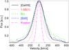 |
Fig. 12 Emission line profiles of [CaVIII], [SiVI], Brγ, (extracted from the nucleus with a circular aperture with a radius of 400 mas), 1-0S(1) (extracted from the eastern H2 region) and a krypton calibration lamp line at 2.148 μm. The spectra were continuum-subtracted by fitting a parabola to wavelength channels to the left and right of the emission lines. In the case of [CaVIII] the continuum was modeled as described in Appendix C to account for absorption of stellar CO bandheads. The emission lines were shifted in velocity to the center of intensity. |
We summarize that we did see [FeII], Brγ and HeI most pronounced along the NLR, with the H2 gas strictly avoiding the NLR. Coronal emission lines indicate a wind and peak a few parsecs to the west of the nucleus. A comparison with the results presented in Storchi-Bergmann et al. (2009) and Storchi-Bergmann et al. (2010) indicates that our observations have a slightly higher angular resolution such that elongated isophotes in the coronal line emission appear to be resolved in our observations (see e.g. the [CaVIII] peak in Fig. 11, top).
6. Dynamics of gas in the NLR
The dynamics of gas in the NLR of NGC 4151 has been subject of various studies, e.g. Crenshaw et al. (2000a), Das et al. (2005) and Storchi-Bergmann et al. (2010). Here, the centroid velocities along the line-of-sight of individual clouds were determined by fitting the emission line profiles with, e.g., multi-Gaussian profiles. The geometry of the volume into which the clouds expand was modeled as a radial outflow where the central obstructing torus confines the flow into a bicone. Assumptions about the mechanism that drives the movement of clouds in the NLR (acceleration or simple ejection) are formulated as the velocity-distance law that relates the radial velocity of clouds with the distance from the nucleus. From the geometry and the velocity distance law one can set up a model to predict possible velocities of clouds in the NLR that can be compared with measured centroid velocities.
The aim of this section is to determine the dynamics of the NLR as traced by [FeII]λ1.6440 μm and to compare our measurements with the results presented in Das et al. (2005) and Storchi-Bergmann et al. (2010). We adopted the geometries and velocity-distance laws presented in these papers and fit two Gaussians to the emission line profiles in our FoV to determine the centroid velocities. We compared the measured centroid velocities and model predictions in terms of position velocity diagrams.
We begin discussing the dynamics of [FeII] with presenting emission line profiles and quantities derived from single-Gaussian fits. Then we discuss channel maps, position velocity diagrams, and results from our fits to emission line profiles in our FoV and compare the found centroid velocities with the model predictions proposed by Das et al. (2005) and Storchi-Bergmann et al. (2010). Finally, channel maps and position velocity diagrams of narrow Brγλ2.166 μm and H2 1-0S(1)λ2.122 μm are presented and discussed.
6.1. Emission line profiles, channel maps, and position velocity diagrams
The emission line profiles of [FeII] in our FoV generally deviate from a single-Gaussian profile (Fig. 13). At distances larger than approximately 0.5 arcsec from the nucleus and along the NLR at a position angle of 60°, line profiles with a component at the systemic velocity of the galaxy and another component that shows up as a blueshifted or redshifted hump to the line profile can be observed. Within our FoV we detect emission at velocities of up to +500 km s-1 in the northeast and up to −250 km s-1 in the southwest. At and around the nucleus the line profile appears to be symmetrical, while at other positions the line profile is composed of two (or more) components.
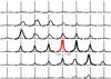 |
Fig. 13 [FeII] emission line profiles extracted from apertures of 385 × 385 mas. [FeII] emission from the nucleus in red. North is up, east to the left. The x-axis represents −1000 km s-1 to +1000 km s-1. The thickness of the emission line profiles scales with flux to guide the eye. |
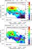 |
Fig. 14 [FeII]λ1.644 μm velocity and dispersion field derived from single-Gaussian fits. The black box indicates our FoV. North is up and east to the left. Gray contours represent [FeII] flux isophotes to guide the eye. Top: [FeII]λ1.644 μm velocity field, 21 cm radio contours in red (.5, 1, 2 and 4 mJy beam-1 with a beam size about four times smaller than our angular sampling) taken from Mundell et al. (2003), and [FeII]λ1.644 μm contours in gray. Numbers in the plot indicate velocities of prominent [OIII] clouds (taken from Kaiser et al. 2000). Bottom: [FeII]λ1.644 μm dispersion field, 21 cm radio contours in red (.5, 1, 2 and 4 mJy beam-1 with a beam size app. four times smaller than our angular sampling) taken from Mundell et al. (2003), and [FeII]λ1.644 μm contours in gray. Numbers in the plot indicate dispersions of prominent [OIII] clouds (taken from Kaiser et al. 2000). |
The velocity and Gaussian dispersion of [FeII] derived from single-Gaussian fits are shown in Fig. 14. The velocities are generally redshifted to the northeast and blueshifted to the southwest with respect to the systemic velocity. At the nucleus the emission generally emerges with systemic velocity. At a distance of 1 arcsec to the nucleus velocity offsets of about 400 km s-1 (see Fig. 14, middle) are observed in the direction of the NLR at a position angle of 60°. Because the most extreme velocities observed in [FeII] exceed those predicted by simple rotation by a factor of 102, this kinematical signature is attributed to an outflow. The derived [FeII] velocities and dispersions together with [OIII]λ501 nm velocities and dispersion from selected clouds taken from Kaiser et al. (2000) are shown in Fig. 14. Velocities and dispersions agree well except that the [OIII] velocities exceed the [FeII] velocities at some very few positions and at the edge of the NLR by several hundred km s-1. These high-velocity [OIII] clouds have been subject to speculations, but because generally the morphology and dynamics of [FeII] and [OIII] are comparable, the excitation mechanism for the two species is the same (photoionization by the central AGN). Generally, the jet may drive this outflow, and the 21 cm radio continuum jet (Mundell et al. 2003) is additionally shown in Fig. 14. The jet is clearly misaligned with the direction of the most extreme velocities in our velocity fields such that the jet may not be the dominant source for the kinematical features observed. Moreover, no increase in dispersion caused by higher turbulance where the jet collides with the ISM is observed (see Fig. 14, bottom). Instead, the dispersion derived from single-Gaussian fits is increased at locations where the [FeII] velocity field shows strong gradients, indicating that the line profile becomes asymmetrical.
To better illustrate the dynamics in [FeII] and its relation to the jet, channel maps and position velocity diagrams of [FeII] are shown in Fig. 15. The channel maps are separated by 100 km s-1, the white contours represent 10%, 25%, 40%, and 55% of the [FeII] peak intensity to guide the eye, and the nucleus is located at position 0, 0. The channel maps centered on −300 km s-1 and +300 km s-1 show an outflow from the nucleus to the southeast directed toward the observer and to the northwest directed away from the observer with prominent emission at systemic velocity. It is possible that the jet locally enhances emission in [FeII], and the 21 cm continuum radio contours are also shown in our channel maps. At about systemic velocity, [FeII] and radio emission correlate at positions F1 and F2. In channel maps centered on high-velocity offsets (e.g. −300 km s-1), the correlation is rather weak such that the high-velocity gas seems to be unaffected by the jet. If emission at systemic velocity is enhanced by the jet, the inclination of the jet must be comparable to the inclination of the galactic disk.
To determine how the velocity of redshifted and blueshifted emission components varies with distance from the nucleus, we assumed that the outflow is directed toward the brightest [FeII] emitting knots at a PA of 60° and constructed the position velocity diagrams shown in Fig. 15. These are extracted from pseudoslits with a width of 0.105 arcsec aligned at a PA of 60° and are offset by multiples of the pseudoslitwidth. For all pseudoslit offsets prominent emission at systemic velocity, i.e., emerging from the galactic disk, is observed. Emission at other velocities along the pseudoslit seems to increase with distance to the nucleus along the pseudoslit. For the pseudoslit centered on the nucleus (Y offset of 0 arcsec), for instance, we observe emission at +400 km s-1 at approximately −1.25 arcsec from the nucleus along the pseudoslit and at −250 km s-1 at a distance of +0.7 arcsec. These numbers indicate that the velocities observed may scale linearly with distance to the nucleus, but we investigate this below in more detail.
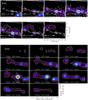 |
Fig. 15 Top: [FeII]λ1.644 μm channel maps. Radio contours overplotted in gray (.5, 1, 2 and 4 mJy beam-1 with a beamsize about four times smaller than our angular sampling). The white contours are 10%, 25%, 40%, and 55% of the [FeII] peak intensity. Velocity ranges are given in km s-1. North is up and east to the left. Bottom: position velocity diagrams of [FeII]λ1.644 μm extracted from pseudoslits oriented along the NLR with a PA of 60°. The Y Offset is the angular offset of the pseudoslit with respect to the nucleus. Along the pseudoslit, position 0 indicates the position of the continuum peak. Contours represent 10%, 25%, 40%, and 55% of the [FeII] peak intensity. |
6.2. Multi-Gaussian fits to the [FeII] emission line profile
To separate the dynamics of the disk from that of the NLR, we followed Das et al. (2005) and Storchi-Bergmann et al. (2010) and decomposed the emission line profiles in the NLR into multiple Gaussians.
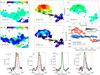 |
Fig. 16 [FeII] dynamics as derived from single- and double-Gaussian fits. All slices with constant wavelength of the datacube were convolved with a Gaussian seeing disk with a FWHM of 0.07 arcsec. The cross denotes the position of the continuum peak. Mayor tick marks in the velocity and dispersion fields correspond to 0.50 arcsec. Letters A to D mark positions from which the spectra shown in the last row were extracted. The black line indicates the position angle of the bicone of 60°. Top: centroid velocities from single-Gaussian fits, VS (left), high/low velocity component from double-Gaussian fits, VH/VL (middle/right). The contours in the middle image in this row represent the 21 cm radio continuum contours (Mundell et al. 2003) at levels of .5, 1, 2, and 4 mJy beam-1 with a beam size about four times smaller than our angular sampling. Middle left and middle: Gausian dispersions of the single- and double-Gaussian fits (σS and σH). Middle right: Centroid velocity of our fits as a function of distance from the continuum peak along the NLR at a position angle of 60°. Black/red/blue points represent the centroid velocities derived from single-Gaussian fits and high- and low-velocity components in case of double-Gaussian fits. Bottom: [FeII] line profiles extracted from various regions with Gaussian fits overplotted. Measured line profile in black, single-Gaussian fits in green, combined double-Gaussian fits in yellow, the low/high velocity component of the double-Gaussian fit in red/blue. |
The spectral resolution of our data allows a decomposition into two Gaussian components, although Das et al. (2005) reported the need for more than three components on selected locations but using spectra with R ≃ 9000. To additionally increase the S/N in our data, each slice of the datacube with constant wavelength was convolved with a Gaussian seeing disk with a FWHM of 0.14 arcsec. The underlying continuum was fitted locally with a parabola in each spectrum and was subtracted before fitting the emission line profile. To facilitate the comparison between this and previous studies, the fit was constrained to a double-Gaussian fit where both Gaussians have an identical FWHM where applicable.
The results of the fits to the [FeII] line profiles are shown in Fig. 16. To illustrate the quality of the fits, emission line profiles and the corresponding fits from selected positions (A−D) in our FoV are also shown. In the case of single-Gaussian fits the centroid velocities VS are usually close to systemic with the exception of the very southwest, close to region F3 (Fig. 16, top left). The single-Gaussian dispersion σS varies between 150 and 200 km s-1, but is increased in regions where the line profile becomes asymmetrical (Fig. 16, middle row, left). In the case of a double-Gaussian fit, the centroid velocities closer to systemic VL (Fig. 16, top row, right) are usually close to systemic too, indicating that emission from the outflowing [FeII] is usually blended with emission from the galactic disk. However, at position A, which corresponds to the western end of region F1, VL deviates from systemic (see the corresponding line profile in Fig. 16, where the component closer to systemic is clearly redshifted). This component cannot be attributed to the jet or the disk but may originate from the front side of the eastern bicone. The centroid velocities farther from systemic VH (Fig. 16, top middle) range from nearly 600 km s-1 at position A to −300 km s-1 at position D (which corresponds to region F3). The derived velocities are typical for emission from the back-side of the eastern bicone especially at position A. It is notheworthy that at position A the dispersion derived from double-Gaussian fits is increased (Fig. 16, middle middle), either due to intrinsically broadened emission or additional unresolved components from the disk. At the brightest [FeII] emission knot in region F1 the radio jet is prominent. Although VH is close to systemic there, it might represent gas that collides with the jet. To investigate whether the gas is accelerated or simply ejected from the nucleus, we show in Fig. 16 (middle right) the derived centroid velocities as a function of distance from the nucleus along the direction of the NLR at a PA of 60°. From this figure acceleration in the NLR cannot be ruled out because the centroid velocities seem to increase with distance at least in the inner 0.5 arcsec. Beyond that radius the velocities seem to increase no more at velocities around 400 km s-1 in the northeast and −250 km s-1 in the southwest. However, to the southwest the dispersion of [FeII] line profiles fitted with a single Gaussian is increased, which implies that the two profile components remain unresolved such that we actually do not see acceleration to the southwest.
6.3. Comparison with existing NLR models
The dynamics of the NLR of NGC 4151 has been the subject of various studies, e.g. Crenshaw et al. (2000a) and Das et al. (2005) who used the STIS slit-spectrograph on-bord the Hubble Space Telescope, and Storchi-Bergmann et al. (2010) who used near-infrared imaging spectroscopy at the GEMINI telescope. The models by Crenshaw et al. (2000a) and more recently by Das et al. (2005) state that [OIII] emission primarily arises from a hollow bicone that is inclined at 45° to the plane of the sky at a PA of 60°. The inner/outer opening angles are 15° and 33° and emission is primarily seen to emerge from between the two bicones. The southwestern part of the bicone points toward the observer, the northeastern part points away from the observer. Because the inclination of the galactic disk is about 22° (with a PA of the line-of-nodes of about 25°, Pedlar et al. 1992), one side of the bicone is more deeply embedded in the galactic disk than the other (see Fig. 17 for the orientation of the galactic disk and the bicone). The [OIII] data presented in Crenshaw et al. (2000a) and Das et al. (2005) indicates acceleration in a nuclear outflow within these two bicones although the origin of this mechanism remains unclear. These authors proposed a velocity-distance law in which the velocity v and the radial distance r to the nucleus are proportional. Acceleration takes place up to a maximum radial velocity of 800 km s-1 at a maximum radial distance of 96 pc. At this distance the ejected material begins to interact with the surrounding interstellar medium such that it decelerates to systemic velocity at a distance of 400 pc. The predicted velocities on the surfaces of the nearer and farther surface of the inner and outer bicone are presented in Fig. 18. In this model, typical velocities observed at that side of the bicone that is closer to the plane of the sky are about 200−300 km s-1, while velocities on the side pointing away from the galactic disk are higher than 500 km s-1.
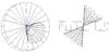 |
Fig. 17 Orientation of the galactic plane and the NLR bicone as they appear on the sky and viewed along the galactic plane of NGC 4151 (according to the model by Das et al. 2005). Only the outer bicone with an opening angle of 33° is shown. |
The models presented by Storchi-Bergmann et al. (2010) are based on the geometry of the model by Das et al. (2005). The authors present position velocity diagrams of [SIII]λ0.9533 μm extracted from pseudoslits extending four arcseconds to either side of the nucleus (see their Fig. 10). These indicate that deviations from the linear velocity-distance law do occur because the gas seems to move with nearly constant velcocity at distances larger than approximately 0.75 arcsec from the nucleus in all pv-diagrams. This motivated the authors to modify the velocity-distance law to a constant with a velocity of 600 km s-1, such that clouds are simply ejected from the nucleus and are not accelerated/decelerated in the NLR. Predicted velocities on the surfaces of the nearer and farther surface of the inner and outer bicone are shown in Fig. 18 (row 2) and the straight, radial isovelocity contours clearly distinguish this model from the acceleration model. But the main difference between the two models becomes more obvious in pv-diagrams extracted from pseudoslits aligned with the mayor axis of the modeled bicone (see Fig. 18, row 3 and 4). The acceleration model allows higher velocities within 0.5 arcsec to the nucleus because the maximum radial velocity in this model is higher than in the constant-velocity model and occurs at the surfaces of the farther/nearer side of the bicone that are closer to our line-of-sight. At larger distances to the nucleus the velocities from the farther and nearer side of the bicone recede to systemic. In contrast, the constant-velocity model predicts constant velocities for all distances to the nucleus only depending on the inclination of the cloud path outward relative to the line-of-sight. Storchi-Bergmann et al. (2010) also presented pv-diagrams of [FeII] in which this constant velocity law is less obvious. However, the morphology and dynamics based on position velocity diagrams of our and their [FeII] observations agree very well, although our FoV only samples the inner 2.5 arcsec. Since the [SIII]λ0.9533 μm emission line is not within our wavelength range, we used the [FeII] emission line instead to trace the dynamics. Furthermore, to facilitate a comparison between our results and the results obtained by Das et al. (2005) and Storchi-Bergmann et al. (2010), we used exactly the same geometry and the same velocity-distance laws as summarized in Table 4.
Geometry and velocity-distance laws.
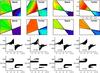 |
Fig. 18 Extreme velocities from the bicone surfaces and position velocity diagrams extracted from the models by Das et al. (2005) and Storchi-Bergmann et al. (2010). Row 1: velocities on the bicone surfaces that are nearer and farther to the observer according to the Das et al. (2005) model. Color scales from −700 km s-1 (blue) to 700 km s-1 (red), contours are in steps of 100 km s-1. Major tick marks correspond to 0.5 arcsec. The surfaces shown cover our FoV. North is up, east to the left. Row 2: same as row 1 for the constant-velocity model by Storchi-Bergmann et al. (2010). Row 3: position velocity diagrams extracted from pseudoslits aligned along the NLR at a position angle of 60° according to the Das et al. (2005) model. The slitwidth/slitlength is 0.15/5 arcsec and the pseudoslits are moved −0.2, 0, 0.2, and 0.4 arcsec away from the nucleus perpendicular to the direction of the NLR. The black area indicates the region in the pv-diagram from which emission is expected according to the model. Note that our observations only cover the inner arcsecond. Row 4: Same as row 3, but for the constant-velocity model by Storchi-Bergmann et al. (2010). |
Figure 19 shows all derived centroid velocities in terms of position velocity diagrams. The pseudoslits are aligned with the modeled bicone and have a width of 0.105 arsec. The green and red contours in this figure are the allowed velocity ranges according to the models by Das et al. (2005) and Storchi-Bergmann et al. (2010). On average, both models cover the same 80% of the allowed velocity ranges for all pseudoslit offsets. The main difference between the models can be observed for pseudoslit offsets around 0.2 arcsec around the nucleus. Here, emission at ±400 km s-1 for distances larger than approximately 0.5 arcsec (depending on the pseudoslit offset) is not expected according to the constant-velocity model, while it is allowed in the acceleration scenario. For positive pseudoslit offsets we actually do observe emission around 400 km s-1 at distances along the pseudoslit of −1.0 arcsec (corresponding to position A and B in Fig. 16), while on the opposite side of the pseudoslit and for comparable negative pseudoslit offsets we only observe velocities around −250 km s-1 (corresponding to position D).
Taking only centroid velocities from the high-velocity component of the double-Gaussian fit and from single-Gaussian fits with velocity offsets greater than 150 km s-1 into account, the acceleration model by Das et al. (2005) complies with 79% of all centroid velocities measured in [FeII], while the constant-velocity model by Storchi-Bergmann et al. (2010) only complies with 66% of all measured centroid velocities. Applying flux values from the individual profile components derived from our fits as weights results in a match of 80% for the Das et al. (2005) model and 74% for the Storchi-Bergmann et al. (2010) model. The velocity signatures of the high-velocity component for all pseudoslit offsets at negative positions along the pseudoslit rather indicate acceleration along the slit up to a position of approximately −1 arcsec Beyond that point, the gas clearly seems to decelerate. Considering the latter and the numbers presented above, we assume that the gas is accelerated within the inner 1 arcsec.
We also checked if the constant-velocity model can be modified that it fits our result better. Changing the ejection velocity only stretches the regions of allowed velocity ranges in the position velocity diagrams such that emission from either positions A and B or D do not match the model. Changing the systemic velocity (redshift) would shift the allowed velocity ranges in the constant-velocity model symmetrically up and down, but this would leave us with the same problems.
The jet may also contribute to the observed low-velocity kinematics of the gas through interactions of the jet with gas in the galactic disk. The blue profiles in Fig. 19 indicate the 21 cm radio intensity within the extracted pseudoslits. The high-velocity gas does not correlate with the radio intensity in the northeast (at negative distances along the pseudoslits) for all pseudoslit offsets but in the southwest (at positive distances along the pseudoslits) for pseudoslit offsets of +0.31 to +0.11 arcsec at distances around +0.75 arcsec. The low-velocity gas seems unaffected except for a pseudoslit offset of −0.21 arcsec at a position of around −1.0 arcsec. This position coincides with the radio knot R2E in Fig. 8. Thus, the jet at least partially enhances emission in [FeII]. The high-velocity components for pseudoslit offsets of +0.21 to 0.00 arcsec at negative pseudoslit positions do not correlate with radio emission. These components are not predicted by the constant-velocity model and cannot be explained in terms of jet enhancements. However, in the acceleration model these components can be explained in terms of gas decelerating because of collisions with the ISM.
In total, the acceleration scenario seems to fit the measured [FeII] kinematics in the inner 1 arcsec better than the constant-velocity scenario.
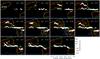 |
Fig. 19 Position velocity diagrams of 0.105 arcsec wide pseudoslits aligned with the NLR at a PA of 60° extracted from the modeled datacube that contains emission from the single- and double-Gaussian fits to the emission line. ΔY denotes the separation of the pseudoslits in arcsec. For ΔY = 0 the pseudoslit covers the nucleus. The green/red contours indicate the allowed regions according to the velocity laws by Das et al. (2005) and Storchi-Bergmann et al. (2010), where tick marks point in the direction of forbidden velocity ranges. The slightly staggered arrangement of the model calculations is not real but is rather due to calculations performed on a grid. The cross marks the center position of the pseudoslit and coincides with the position of the nucleus. 21 cm radio continuum emission along the pseudoslits is plotted in blue. |
6.4. Dynamics in Brγ and H2
Channel maps and pv-diagrams of Brγ and H2 are presented in Figs. 20 and 21. In contrast to [FeII], the Brγ channel maps appear to be less clumpy and emission primarily emerges with systemic velcocity extending toward a PA of approximately 80°. A low-velocity component at about −250 km s-1 can be observed that spatially and dynamically coincides with the southwestern [FeII] knot 60 pc to the west, but the correlation between the [FeII] and Brγ channel maps, especially to the northeast of the nucleus, is low. Instead, emission emerging with about +200 km s-1 nearly north to the nucleus at a PA of 20° can be observed. This region is still located within the NLR and may be attributed to the outflow. It is noteworthy that the Brγ channel maps presented by Storchi-Bergmann et al. (2010) show the very same behavior. Further in, at the position of nucleus, the slightly curved isophotes in the pv-diagram (for a Y offset of 0 arcsec) may indicate an inflow. This inflow can also be observed in the inset of Fig. 22, where the Brγ velocity field as derived from single-Gaussian fits is shown. The inflow can be traced to either side of the nucleus up to distances of about 20 parsecs at a PA of −45°, which is nearly perpendicular to the outflow observed in [FeII] and deviates only about ~20° from the PA of the mayor H2 emitting regions. The orientation of the galactic disk (see Fig. 17) is well compatible with an inflow within the galactic disk maybe from the larger H2 reservoirs seen in Fig. 21. However, the symmetry of the velocity signature may also imply a rotating but dynamically decoupled disk around the black hole. Considering the angular resolutions provided by our observations, it is hardly possible to distinguish the two scenarios.
The H2 gas morphology is completely different from Brγ or [FeII]. H2 seems to emerge primarily at systemic velocity, thus from within the disk, but avoiding the NLR. At the position of the low-velocity component at −250 km s-1 seen in Brγ and [FeII], H2 emission at about the same velocity is observed, but not the increase in velocity to the north of the nucleus. Investigating the H2 channel maps presented by Storchi-Bergmann et al. (2010) we see the same behaviour (see their channel map centered on −270 km s-1). To investigate the dynamics in Brγ and H2 in more detail, we fitted the emission line profiles with a double Gaussian. The results are shown in Figs. 23 and 24. The emission line profiles at the position of the bright western [FeII] knot are clearly double-peaked with one profile component at systemic and another at about −250 km s-1, i.e., similar to what is observed in [FeII]. Again, emission at systemic and/or low velocities at this position may be locally enhanced by the jet. To the north the Gaussian dispersion in Brγ is increased (see Fig. 23, Brγ line profile at position J), indicating that the individual profile components remain spectrally unresolved.
7. Column densities and excitation mechanisms
In this section we investigate the excitation mechanism of hot H2 and derive column densities and the total mass of hot H2. We furthermore determine the mass of ionized hydrogen and estimate a lower limit of the column density of the HeI 21S state.
7.1. H2
7.1.1. Column densities and population density diagram
Because there is little H2 emission from inside the NLR bicone, it is reasonable to assume that the H2 molecules dissociate in the radiation field of the AGN while H2 molecules, for which the AGN is hidden behind the putative molecular torus, survive and are excited. The emission of H2 is most pronounced along the direction of the resolved flux density ratio map (Fig. 4), which roughly coincides with the bar.
Storchi-Bergmann et al. (2009) detected more than 10 H2 emission lines from J to K band and concluded from a population-level diagram that a thermal excitation mechanism dominates. In our spectra only the 1−0 series is detectable with high confidence, although emission from the 2−1 series is detectable with lower confidence.
The column density can be derived from 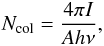 (Beckwith et al. 1978) where I is the
measured surface brightness in the line and A is the Einstein A
coefficient for that transition. Table 2 lists
the measured fluxes for our whole FoV. The derived column densities (see Table 5) are all lower than 1016
cm-2, characteristic for optically thin H2 regions.
(Beckwith et al. 1978) where I is the
measured surface brightness in the line and A is the Einstein A
coefficient for that transition. Table 2 lists
the measured fluxes for our whole FoV. The derived column densities (see Table 5) are all lower than 1016
cm-2, characteristic for optically thin H2 regions.
Detected species, transition probabilities (Turner et al. 1977), degeneracy, upper level energy, and derived column densities for our whole FoV.
The population-level diagram reveals a thermal excitation mechanism with a temperature of about 1700 K using all species (see Fig. 25) and 1500 K using 1−0 species only. Since our H2 fluxes were not corrected for reddening, the derived excitation temperature may be a lower limit.
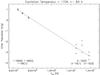 |
Fig. 25 Population density as function of upper level energy. Triangles denote data points, error limits are indicated by crosses. |
7.1.2. Diagnostics of excitation mechanisms
Mouri (1994) proposed to use ratios involving ro-vib transitions of H2 to distinguish the dominant excitation mechanisms. The measured ratios of 2-1S(1)/1-0S(1) and 1-0S(2)/1-0S(0) (see Fig. 26) imply that shock (J-shock model from Brand et al. 1989) and X-ray excitation are favored, which we investigate in more detail in the following.
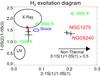 |
Fig. 26 “Mouri diagram”. The data regions correspond to shocks (Brand et al. 1989), non-thermal (Black & van Dishoeck 1987) and thermal UV (Sternberg & Dalgarno 1989), and X-ray (Lepp & McCray 1983; Draine & Woods 1990). The diamond corresponds to data extracted from our whole FoV, the triangle to data extracted from the bright H2 knot in the east, and stars to data from other galaxies (NGC 1275 and NGC 6240 taken from Krabbe et al. 2000). The red arrow shows the displacement for a reddening correction of AK = 1. |
We used the models of Maloney et al. (1996) to
compare observed and predicted 1−0S(1), 2−1S(1) and [FeII]λ 1.644
μm fluxes in XDRs. Their Fig. 6 summarizes derived intensities for
the above species as a function of the effective (attenuated) ionization parameter
ζeff, which is defined as
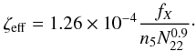 Here
n5 [105 cm-3] is the density of
hydrogen nuclei in the emitting cloud, fX [erg
cm-2 s-1] the flux of X-rays penetrating the cloud, and
N22 [1022 cm-2] the total
attenuating hydrogen column density. Cappi et al.
(2006) found an X-ray flux of FX(2−10 keV) =
4.5 × 10⁻¹⁴ W m-2 and an attenuating column density of
N = 7.5 × 1022 cm-2. Assuming isotropic X-ray
emission, we find
Here
n5 [105 cm-3] is the density of
hydrogen nuclei in the emitting cloud, fX [erg
cm-2 s-1] the flux of X-rays penetrating the cloud, and
N22 [1022 cm-2] the total
attenuating hydrogen column density. Cappi et al.
(2006) found an X-ray flux of FX(2−10 keV) =
4.5 × 10⁻¹⁴ W m-2 and an attenuating column density of
N = 7.5 × 1022 cm-2. Assuming isotropic X-ray
emission, we find 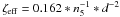 ,
where d [pc] is the distance of a H2 cloud from the nucleus. Table 6 lists predicted 1-0S(1) fluxes per spaxel as a
function of ζeff and hydrogen densities of
n5 = 0.01 and n5 = 1. For
typical distances d of a few dozen parsecs, ζeff is
generally lower than 0.01. Comparing ζeff with Fig. 6 of
Maloney et al. (1996) reveals that the
predicted 1-0S(1) fluxes are generally lower than s10-21 W m-2,
which is at least two orders of magnitude lower than the highest observed 1−0S(1) flux.
,
where d [pc] is the distance of a H2 cloud from the nucleus. Table 6 lists predicted 1-0S(1) fluxes per spaxel as a
function of ζeff and hydrogen densities of
n5 = 0.01 and n5 = 1. For
typical distances d of a few dozen parsecs, ζeff is
generally lower than 0.01. Comparing ζeff with Fig. 6 of
Maloney et al. (1996) reveals that the
predicted 1-0S(1) fluxes are generally lower than s10-21 W m-2,
which is at least two orders of magnitude lower than the highest observed 1−0S(1) flux.
Theoretical flux values for 1-0S(1) in W/m2 emerging from a spaxel of 50 × 50 mas as a function of the hydrogen density and distance from the nucleus and hence ζeff from Fig. 6 of Maloney et al. (1996).
Using [FeII] flux values from Storchi-Bergmann et al. (2009) extracted from a 0.3 × 0.3 arcsec aperture at the position of the bright eastern H2 knot (see their table 1) reveals a measured ratio of 1-0S(1)/[FeII] of about 0.9. In the models of Maloney et al. (1996) this requires ζeffs0.1, for which the predicted 1-0S(1) flux would also be close to the observed flux values. Therefore X-ray excitation might be the dominant excitation mechanism if the emission of X-rays is not isotropic, implying higher ζeff at the position of the H2 clouds. We might now speculate that the central absorber is perforated. In this case some H2 regions could be more directly exposed to radiation from the central engine (which remains unresolved by our observations) with the nucleus hidden by the central absorber along our line-of-sight. However, the X-ray emission as traced by high-ionization lines appears rather confined to the narrow line region (Ogle et al. 2000), which is partially embedded in the galactic disk. If we assume that the radio jet is roughly perpendicular to the putative molecular torus, the torus is highly inclined with respect to the galactic plane. In this case the central engine is nearly hidden by the torus along our line-of-sight, giving rise to the high attenuating column density observed by Cappi et al. (2006), but H2 regions in the galactic disk are much more exposed to the nuclear radiation field. We therefore conclude that X-rays might contribute significantly to the H2 and [FeII] emission observed.
On the other hand, 1-0S(1) and [FeII] emission can be strong in shocks from supernova explosions into the interstellar medium. Following Hollenbach & McKee (1989) (their Figs. 5 and 8) the line ratio 1-0S(1)/[FeII] is about unity for shock velocities above 40 km s-1. These shocks, if present, may rather be induced by the bar than by supernova remnants since the 6 cm radio emission morphology is more aligned with the 21 cm radio jet (see e.g. Ulvestad et al. 1981) and clear signs of massive starformation in the central 100 pc remain undiscovered.
Thus, we conclude that excitation by X-rays and shock excitation especially along the bar contribute to the H2 and [FeII] fluxes observed. According to Fig. 26, X-ray excitation in NGC 4151 may even be more dominant than in the Seyfert 1.5 galaxy NGC 1275 or the ultra-luminous infrared galaxy NGC 6240.
7.1.3. Total mass of molecular and ionized gas
The luminosity in, e.g., 1-0S(1) is given by  where
L1−0S(1) is the luminosity in 1−0S(1),
n0 is the number of H2 molecules,
gJ the statistical weight for that
transition, E1−0S(1) the energy of the
upper level, Z(T) the partition function,
T the temperature,
A1−0S(1) the Einstein A coefficient of
the 1-0S(1) transition, and ν the frequency of the emitted photon. The
partition function is taken from Irwin (1987).
The total 1-0S(1) flux in our FoV is
F = 2.9 × 10⁻¹⁷ W/m2.
Assuming a distance of d = 13.25 Mpc and a temperature of 1700 K, we
obtain a mass of hot molecular H2 of
MH2 = 100 M⊙,
which also fully complies with the measurements by Storchi-Bergmann et al. (2009). Since our FoV does not fully sample the whole
inner region, the derived hot H2 mass is a lower limit. This amount is also
rather small, but as Dale et al. (2005) point
out, the hot-to-cold mass ratio in centers of galaxies ranges between 10-7
and 10-5, which matches the high gas concentrations of
s108 M⊙ as inferred from mm-observations (NGC
4569: Boone et al. 2007; NGC 6951: Krips et al. 2007 and others for the NUclei of
GAlaxies (NUGA) group). Thus the total amount of molecular gas in the central 100 pc of
NGC 4151 may be higher by several orders of magnitude.
where
L1−0S(1) is the luminosity in 1−0S(1),
n0 is the number of H2 molecules,
gJ the statistical weight for that
transition, E1−0S(1) the energy of the
upper level, Z(T) the partition function,
T the temperature,
A1−0S(1) the Einstein A coefficient of
the 1-0S(1) transition, and ν the frequency of the emitted photon. The
partition function is taken from Irwin (1987).
The total 1-0S(1) flux in our FoV is
F = 2.9 × 10⁻¹⁷ W/m2.
Assuming a distance of d = 13.25 Mpc and a temperature of 1700 K, we
obtain a mass of hot molecular H2 of
MH2 = 100 M⊙,
which also fully complies with the measurements by Storchi-Bergmann et al. (2009). Since our FoV does not fully sample the whole
inner region, the derived hot H2 mass is a lower limit. This amount is also
rather small, but as Dale et al. (2005) point
out, the hot-to-cold mass ratio in centers of galaxies ranges between 10-7
and 10-5, which matches the high gas concentrations of
s108 M⊙ as inferred from mm-observations (NGC
4569: Boone et al. 2007; NGC 6951: Krips et al. 2007 and others for the NUclei of
GAlaxies (NUGA) group). Thus the total amount of molecular gas in the central 100 pc of
NGC 4151 may be higher by several orders of magnitude.
Following Riffel et al. (2008); Scoville et al. (1982), the amount of ionized gas can
be estimated: 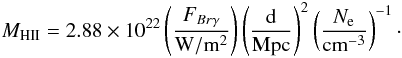 Assuming
an electron density of Ne = 100 cm-3 and using
the total narrow Brγ flux of
FBrγ = 4 × 10-17 W/m2,
a total ionized hydrogen gas mass of
M = 2.1 × 10⁶ M⊙ can be
derived, which fully agrees with the measurements by Storchi-Bergmann et al. (2009).
Assuming
an electron density of Ne = 100 cm-3 and using
the total narrow Brγ flux of
FBrγ = 4 × 10-17 W/m2,
a total ionized hydrogen gas mass of
M = 2.1 × 10⁶ M⊙ can be
derived, which fully agrees with the measurements by Storchi-Bergmann et al. (2009).
7.2. A lower limit to the HeI 21S column density
As shown in Fig. 10, the HeI emission is extended while the flux in the absorption component decreases exactly with the strength of the continuum emission. Furthermore, the velocity offset of this absorption complex remains constant throughout our FoV, and we assume that the absorption component is related to a nuclear outflow that remains spatially unresolved. The whole line complex appears P-Cygni-like with a symmetrical absorption component and no broad emission component. The velocity offset of the HeI absorption component is −280 km s-1 with a lorentzian HWHM of 400 km s-1 and an equivalent width of 7.7 Å. These numbers differ from the velocities and FWHMs of absorption in UV resonance lines, see Table 1 of Kraemer et al. (2001). These authors used photoionization models to determine, e.g., the distance of individual absorbers along the line-of-sight. As a result, absorption is usually broadened (FWHM higher than 430 km s-1) for clouds closer than 1 pc to the nucleus, but these clouds (D+E and D’) also have outflow velocities higher than about 500 km s-1. Furthermore, Balmer and HeIλ3888 Å absorption is not seen as a multi-component absorber as in the UV and the outflow velocities increase in nuclear high states (Hutchings et al. 2002), which has not been observed in the UV lines. This may indicate that our HeI absorption originates from a different region than the observed UV resonance lines. Since the opening cone of the ionizing radiation is close to the line-of-sight, it is reasonable to assume erosion of the edge of the obscuring torus.
The blueshifted optically thin absorption component in the HeI profiles of our nuclear spectra (see Fig. 9, top) can be used to calculate the HeI 21S column density. Since only one of the many prominent transitions from the lower HeI 21S level is covered by our observations, this yields a lower limit to the column density of the HeI 21S level. Figure 27 shows a Grotrian diagram of HeI labeled with some prominent astronomical transitions including the transitions from and to the 21S level. The lowest singlet level 21S and especially the lowest triplet level 23S are both metastable with transition probabilities of 51.3 s-1 and 1.27 × 10⁻⁴ s-1 to the ground state, 11S. Depopulation of these levels can take place by photoionization or by the highly forbidden emission of high-eV photons to the ground state. Absorption of λ3889 Å photons by 23S leads to enhanced emission of λ10830 Å. Radiatively pumping the ground state 11S to 21P by absorption of λ584 Å photons may be essential to produce emission of λ20581 Å because the decay of 21P by re-emitting a photon of the same wavelength is highly favored (99.9%) against the emission of a λ20581 Å photon (Robbins & Bernat 1974). However, the λ20581 Å line strength is limited by photoionization of hydrogen by the λ584 Å photon (Thompson & Tokunaga 1980). Moreover, collisional excitation of the more long-living level 23S to 21S may be of importance as well (see e.g. Osterbrock 1989).
The total column density of 21S can be estimated using additional absorption lines such as λ3965 Å or λ5016 Å. Unfortunately, these lines are blended with Hϵ, [NIII], and [OIII] and are also not covered by our observations. Here we confine ourselves to calculating a lower limit of the 21S column density following Hamann et al. (1997) and Crenshaw et al. (1999).
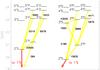 |
Fig. 27 Grotrian diagram of HeI. Prominent astronomical lines (plotted in yellow) are indicated with wavelengths in Å. Transitions from metastable levels to the ground state are plotted in red. |
The underlying continuum was fitted with a parabola using spectral channels to the
shorter and longer wavelength side of the line complex, and we normalized each spectrum by
dividing with the underlying continuum emission. Ir is then
the residual flux at a particular radial velocity vr. The
minimum covering factor Clos in the line-of-sight, the
fraction of continuum that is absorbed by the occulter, is then
Clos > = 1−Ir.
Assuming screen extinction, the optical depth τ is then given by
τ = ln (1/Ir)
if the covering factor is one,
τ = ln (Clos/(Ir + Clos + 1)
otherwise. The column density N is then obtained by integrating the optical depth across
the line profile,  with
λ the laboratory wavelength, me the
electron mass, c the speed of light, e the electron charge and
f12 the (absorption) oscillator strength, where
f12 = 0.375 (Wiese &
Fuhr 2009). Assuming screen extinction and a covering factor of
Clos = 1, we derive a column density of 5 × 10¹²
cm-2. The minimum covering factor derived is
Clos = 0.09, which increases the column density to
1 × 1014 cm-2. The f-value of the HeI 10830 Å
transition is about 0.18 and consequently comparable with the f-value of
the HeIλ20581 Å transition. Since the transition probability for
radiative decay of the 23S level is lower by a factor of
10-5 than for the 21S level, and assuming that
the population density of the 23S and
21S levels differ by a similar factor, we expect a similarly
deep HeIλ10830 Å absorption complex, which is indeed observed (Storchi-Bergmann et al. 2009).
with
λ the laboratory wavelength, me the
electron mass, c the speed of light, e the electron charge and
f12 the (absorption) oscillator strength, where
f12 = 0.375 (Wiese &
Fuhr 2009). Assuming screen extinction and a covering factor of
Clos = 1, we derive a column density of 5 × 10¹²
cm-2. The minimum covering factor derived is
Clos = 0.09, which increases the column density to
1 × 1014 cm-2. The f-value of the HeI 10830 Å
transition is about 0.18 and consequently comparable with the f-value of
the HeIλ20581 Å transition. Since the transition probability for
radiative decay of the 23S level is lower by a factor of
10-5 than for the 21S level, and assuming that
the population density of the 23S and
21S levels differ by a similar factor, we expect a similarly
deep HeIλ10830 Å absorption complex, which is indeed observed (Storchi-Bergmann et al. 2009).
8. Summary
We have used near-infrared integral field data obtained with OSIRIS at the Keck telescope to determine the morphology and dynamics of ionized and molecular gas in the inner two arcseconds of NGC 4151. We compared our results with previous measurements by Das et al. (2005) and Storchi-Bergmann et al. (2010). The main results can be summarized as follows:
-
a)
The stellar and non-stellar contributions to the total continuumboth peak at the same position and remain unresolved by ourobservations. Brγ and coronal lines peak a few parsec to the northwest/west of the continuum peak. Coronal lines also show a broad component implying that these species may originate from an outflow.
-
b)
The ionized gas extends toward the NLR while the molecular gas strictly avoids the NLR. The NLR morphology is well compatible with measurements by Storchi-Bergmann et al. (2010).
-
c)
We identified four dynamical components. First, emission at systemic velocity, which is assumed to emerge from the galactic disk of NGC 4151. Second, emission that is enhanced due to interaction with the jet. Third, a nuclear inflow of gas (most likely within the galactic disk) that is observed in Brγ. And fourth, an outflow along the NLR bicone.
-
d)
The outflow of the NLR gas as traced by [FeII] is well compatible with the models proposed by Das et al. (2005) (the acceleration model) and Storchi-Bergmann et al. (2010) (the constant-velocity model). We emphasize that our FoV is smaller than the FoV provided in Storchi-Bergmann et al. (2010) so that we are unable to confirm or reject their constant-velocity model for distances larger than approximately one arcsecond from the nucleus. However, our data indicate acceleration within the central arcsecond, which agrees with the model proposed by Das et al. (2005).
-
e)
The 21 cm radio continuum jet originates from regions where H2 gas is rotating into the path of the jet because of the galactic rotation. The jet also interacts with gas at certain positions and locally enhances emission of [FeII].
-
f)
The hot H2 gas appears to be thermal with a temperature of about 1700 K, and X-ray and shock excitation of H2 are very likely to occur. Derived column densities are about 1014 cm-2. We detected a bridge of H2 running through the nucleus. Although the velocities along this bridge are systemic, we observed inflow in Brγ at speeds that match with speeds expected at the radius of the sphere of influence.
-
g)
We detected HeI emission that is accompanied by a blueshifted optically thin absorption component in our nuclear spectra. The absorption component has a velocity offset of −280 km s-1 and remains spatially unresolved. We assume that this feature represents a nuclear outflow that occurs closer than a very few parsecs to the nucleus. We calculated a covering factor of Clos = 0.09 with a minimum column density of 1 × 1014 cm-2 for the HeI 21S level.
Online material
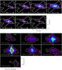 |
Fig. 20 Brγ channel maps and position velocity diagrams. Prior to extraction all slices with constant wavelength of the datacube were convolved with a Gaussian seeing disk with a FWHM of 0.10 arcsec. Top: channel maps. 21 cm radio contours in gray (.5, 1, 2, and 4 mJy beam-1 with a beam size about four times smaller than our angular sampling) and the white contours are 10%, 25%, 40%, and 55% of the Brγ peak intensity. Velocity ranges are given in km s-1. North is up and east to the left. Bottom: Position velocity diagrams extracted from pseudoslits oriented from east to west. The Y offset is the angular offset of the pseudoslit with respect to the nucleus. Along the pseudoslit, position 0 indicates the position of the continuum peak. Contours represent 10%, 25%, 40%, and 55% of the Brγ peak intensity. |
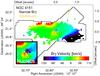 |
Fig. 22 Brγ velocity field derived from single-Gaussian fits to the line profile extracted from every spaxel with continuum contours (20% and 50% of the peak value) in yellow. The inset shows the Brγ velocity field on the nucleus scaled in velocity from −75 km s-1 (blue) to 75 km s-1 (red). |
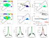 |
Fig. 23 Same as Fig. 16, but for Brγ. All slices with constant wavelength of the datacube were convolved with a Gaussian seeing disk with a FWHM of 0.2 arcsec. |
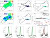 |
Fig. 24 Same as Fig. 16, but for 1-0S(1). All slices with constant wavelength of the datacube were convolved with a Gaussian seeing disk with a FWHM of 0.15 arcsec. |
Appendix A: Data reduction software
The data reduction software package consists of the data reduction pipeline that performs all necessary basic steps to provide the user with a standardized data cube and graphical user interfaces (GUI) to plan the reduction strategy. The package is IDL-based (version 6.0 and higher, IDL is a product from ITT Visual Information Solutions) with some reduction steps programmed in C for reasons of computation speed. The GUIs are Java-based. The data reduction scheme itself is modular, providing individual reduction steps for individual tasks such as sky subtraction, etc. The reduction scheme is coded as an XML-file and interpreted and executed by the backbone part of the software package. More detailed information about the data and command flow can be found in Krabbe et al. (2004). We point out that some of the data reduction recipes below were specifically designed for reducing commissioning data of the OSIRIS instrument. A comprehensive compendium of data reduction strategies and a description of the current data reduction pipeline can be found in the OSIRIS user manual.
Appendix A.1: Data reduction
Appendix A.1.1: Microlens arrays and the arrangement of spectra on the detector
A key device in integral field spectrographs is the image slicer that samples and rearranges the field-of-view of the instrument in the focal plane to create the entrance slit for the actual spectrograph. Various designs for this device have been established. The most common ones for sampling the focal plane are optical fibers, plane mirror slicers, and microlens arrays.
In OSIRIS, a microlens array samples the focal plane with an array of small lenses. Each rectangular microlens has a width of 200 μm and focuses the light onto a pupil image that is significantly smaller than the microlens’ diameter. These images are then fed into the actual spectrograph. Overlapping of the individual spectra on the detector is avoided by rotating the microlens array by 3.6° relative to the dispersion axis of the grating, which itself is aligned with the rows of the detector. As a side effect, the spectra run diagonally across the detector rows at the same angle. The arrangement of the spectra on the detector is staggered (see Fig. A.1 for a sky-subtracted detector image of NGC 4151). In OSIRIS, spectra from adjacent microlenses of a row are shifted horizontally (along the dispersion axis) by roughly 30 detector pixels, have a FWHM of two detector pixels perpendicular to it and are separated by two detector pixel.
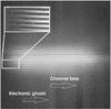 |
Fig. A.1 Sky-subtracted detector image of NGC4151. The dispersion axis runs horizontally. Various electronic effects can be identified, such as bias variations in the multiplexer readout channels and electronic ghosts. The staggered arrangement of the spectra can also be seen in the inset. |
Appendix A.1.2: Reconstruction of the light distribution in the microlens array
The heart of each data reduction software for integral field spectrographs is the reconstruction of the incident light on the slicer from the recorded detector raw images via a mapping function. When using fibers or microlens arrays each point spread function (PSF) of every fiber/microlens and their location on the detector must be determined to reconstruct the distribution of incident light on the slicer. In OSIRIS, a movable scanning mask allows illumination of exactly one microlens column. Illuminating the mask with a whitelight source results in continuum spectra that are well separated on the detector. From the measured PSFs the so-called rectification matrix is assembled, which contains spatially and spectrally the contribution of every microlens to the signal detected in any detector pixel. This procedure is part of the instruments calibration and is performed during daytime. Mathematically, for a given column or a given wavelength, the recorded signal in a detector pixel in row i is Di. We consider Ik to be the incident light on the kth microlens and Mik the rectification matrix mapping how much light from the k-th microlens is focused to the ith detector pixel in the given row: Di = Mik × Ik. Since the detector has 2048 rows, Di is a vector with 2048 elements. The number of microlenses in a given observing mode is n, so Ik is a vector with n elements. The rectification matrix itself therefore has 2048 × n elements (for that given detector column). To solve for Ik this matrix equation is inverted with an iterative Gauss-Seidel algorithm in a process hereafter called “rectification”.
Since every microlens is illuminated with same intensity and spectrum, the rectification matrix already accounts for the flatfield, making an additional flatfielding step obsolete.
Appendix A.1.3: Notes on selected reduction steps
An updated and more complete list of reduction recipes including some experimental ones can also be found in the OSIRIS user manual (Larkin et al. 2008). Here we only summarize special reduction steps in the order applied to our data sets obtained during the first commissioning run of OSIRIS.
Time-variable DC biases in the multiplexer readout channels
The Hawaii II detector is equipped with eight readout channels (128 × 1024 detector pixels) per quadrant. The channels run horizontally in the upper right and lower left quadrant and vertically in the other quadrants (the dispersion axis runs horizontally on the detector). Occasionally, the readout electronics introduces time-variable DC biases in these channels that do not always cancel out in sky-subtraction, resulting in residual biases of several % of the maximum signal. An automatic correction of these residual biases is only possible in dark areas of the detector (the very left and very right of the detector) and horizontal channels (the lower left and upper right quadrants). For the other quadrants we developed a manual correction method that assumes that all measured continua with similar horizontal shift are similar to each other, except for scaling, an assumption that fairly well holds for our observation except for the bright AGN itself. In the lower/upper half of the detector the first/second half of a spectrum crosses eight channels while the other half lies within one channel. Summing all spectra with similar horizontal shift of the lower and of the upper half of the detector and comparing them to each other reveals well-defined steps in the two spectra, which are due to the mentioned channel biases.
Electronic ghosts
Detector rows running along the fast-clock direction of the channel that are highly discharged (having a high signal) are sometimes reproduced at a lower signal level in other channels along their fast-clock direction. This indicates that this crosstalk between channels is due to the readout electronics. Since the alignment of the channels is vertical in the upper left and lower right quadrant and horizontal in the others, this crosstalk (electronic ghosts) may cross spectra on the detector, faking emission lines. Our method seems to be the most suitable for our commissioning data. Here, we median 50 rows at the bottom and at the top of the detector vertically, shift the resulting vectors by a few detector pixels horizontally, and subtract them from each other. The difference should be around zero with electronic ghosts showing up as positive peaks. Their value and position can easily be determined and then subtracted.
Bad-pixel interpolation in raw data
Owing to the staggered arrangement of the spectra on the detector, bad pixels can only be interpolated in the raw image along the dispersion axis. Depending on how many consecutive pixels need interpolation, the interpolation is quadratic (isolated bad pixels) or linear (clusters of bad pixels). Transient bad pixels in commissioning data require special attention. If a pixel is bad in the rectification matrix but not in the detector image, rectification may in some cases diverges giving useless results for the whole microlens column at that wavelength, requiring interpolations in the matrix as well3.
Wavelength calibration
Wavelength calibration is performed using neon, argon, krypton, and xenon calibration lamps that illuminate the entrance pupil of the instrument. Each spectrum is wavelength-calibrated individually. First, the known emission lines are fitted with a Gaussian, then the fitted center positions are interpolated with a cubic dispersion function. Interpolation onto a regular wavelength grid is done linearly with a grid width close to the intrinsic sampling of each filter band. The accuracy of the wavelength calibration was determined to be 2/10th of a detector pixel (10 km s-1) around 2.1 μm4.
Bad-pixel identification and interpolation in data cubes
Once a data cube is assembled, we can take the advantage of the fact that neighboring angular resolution elements (spaxels) carry similar astronomical information. For any given spaxel all spectra of neighboring spaxels are scaled in intensity to the spectrum of the central spaxel. Any data element of a spectrum (spexel) that deviates by more than 3σ from the median of all scaled spectra is considered as bad. Linear interpolation is then performed along all three axes and the three interpolated values are averaged.
Correction of imbalanced sky subtraction
Biases in sky-subtracted spectra, resulting from slightly imbalanced sky subtraction or residual biases in the multiplexer readout channels, can cause residuals when these spectra are divided by the telluric spectrum especially in the atmospheric transmission valleys between 2.00 and 2.08 μm. We subsequently added a bias to each spectrum, divided by the telluric spectrum, and fitted the result where the spectrum is free of emission and absorption lines and where the transmission of the atmosphere is higher than 40%, linearly. Assuming a linear continuum in this small wavelength range, the appropriate bias was found when the difference between the fit and the divided spectrum was the smallest. This bias was then added to the whole spectrum.
Mosaicking
Prior to mosaicking all data cubes are rotated to a common PA by spatially oversampling each pixel and resampling to a new rotated grid. α,δ offsets are determined from images created by collapsing the data cubes along the λ-axis and cross-correlating them using the correl_optimize routine from astrolib (Landsman 1993). The shifted datasets are finally added.
Appendix B: Influence of variable seeing on mosaics of data cubes
The distribution of flux in a typical PSF of an AO system shows two components, a diffraction-limited spike on top of a more extended Gaussian seeing base. Under different seeing conditions or different AO performances these two components are pronounced and extended differently. However, the PSF should be radially symmetrical. We obtained our five K-broadband data cubes under quite different seeing conditions. When combining the individual data cubes, circular radial profiles are only preserved in a region where all data cubes overlap, the central arcsecond around the bright AGN. Regions where only a fraction of the data cubes overlap are dominated by the combined radial flux distribution of those data cubes involved. Due to the rectangular shape of our FOV, the radial intensity profiles in the legs of the x-shaped mosaic are clearly dominated by the prevailing seeing conditions at the time of observation of the data cubes involved. Since the horizontal strip was obtained under poorer seeing conditions than the tilted strip, the combined radial profile has become of elongated shape, although intrinsically, the radial continuum profile is circular on this scale, see Peletier et al. (1999).
While mosaics of data cubes that contain extended emission suffer from variable seeing in the non-overlapping regions, localized emission of higher spatial frequency such as the nucleus are much less effected by seeing variations. Their shape is that of the combined PSF spikes and their locations within the FOV remain unchanged. As a result, under variable seeing conditions, localized emission and absorption features can reliably be traced throughout the combined data cube, while extended emission can only be reliably traced within the area shared by all contributing data cubes. We are therefore restricting our analysis of extended structures like the continuum to the central region in Fig. 3.
Appendix C: Spectral decomposition
The decompositioning algorithm is based on the algorithm presented in Krabbe et al. (2000). In active and starburst
galaxies, one can identify at least four sources of continuum emission: stellar
( ), AGN
power-law (
), AGN
power-law ( ), hot
dust (
), hot
dust ( ), and
free-free (
), and
free-free ( )
emission. The intrinsic continuum emission
)
emission. The intrinsic continuum emission  at each
wavelength is
at each
wavelength is  (C.1)where
wS, wP,
wD, and wFF represent the
contributions of the individual sources. A synthetic continuum spectrum
ISynth. can be constructed by
additionally applying extinction. Here, we define the optical depth
τ(λ,k) with the reddening parameter
k as
τ = kλ-1.85 (Landini et al. 1984) and apply a screen model. We now
construct a synthetic spectrum for every measured
(C.1)where
wS, wP,
wD, and wFF represent the
contributions of the individual sources. A synthetic continuum spectrum
ISynth. can be constructed by
additionally applying extinction. Here, we define the optical depth
τ(λ,k) with the reddening parameter
k as
τ = kλ-1.85 (Landini et al. 1984) and apply a screen model. We now
construct a synthetic spectrum for every measured
spectrum that fits best in terms of minimal χ2 difference. Wavelengths with prominent emission/absorption lines due to non-continuum sources (e.g. shocked ISM gas, photoionized gas clouds) are not considered in the χ2 calculations.
The stellar component of the continuum emission was modeled using normalized stellar
K-band spectra of Wallace &
Hinkle (1997). The spectral resolution of our data was downsampled to the
resolution of our stellar template spectrum of HR8726, a K5Ib supergiant. The stellar
template spectrum was additionally redshifted and velocity broadened by convolving it
with a Gaussian line-of-sight velocity profile. The AGN power-law emission was assumed
to vary as  with the spectral
index α. Emission from hot dust of temperature T was taken to be a
black body Bλ(T)
multiplied by a power-law emissivity of the form
ϵDust ∝ λ-1. Additionally, we
assumed that the amount of extinction and the amount of emission from hot dust are
correlated
with the spectral
index α. Emission from hot dust of temperature T was taken to be a
black body Bλ(T)
multiplied by a power-law emissivity of the form
ϵDust ∝ λ-1. Additionally, we
assumed that the amount of extinction and the amount of emission from hot dust are
correlated  ,
giving
,
giving  .
.
For reasons mentioned above, we ignored eventual free-free emission in our calculations and limited the wavelength range when decomposing to 2.25 to 2.36 micron. The complete set of fit parameters is wS, wP, wD, k, α, T, the stellar redshift z, and the stellar velocity dispersion σ. To increase the signal-to-noise ratio we convolved each slice of the datacube with constant wavelength with a Gaussian seeing disk with a FWHM of 100 mas.
The Keck adaptive optics system uses a Shack-Hartmann wavefront sensor in the visible spectrum.
Assuming that the dynamics is dominated by a massive point-like object at the position of the nucleus with a mass of 5 × 10⁷ M⊙, see e.g. Onken et al. (2007), the rotational velocity for an edge-on disk at a projected radial distance of 70 pc is only 56 km s-1 instead of the observed 500 km s-1.
In more recent versions of the rectification algorithm for data taken after the first commissioning run we take full advantage of the fact that the spectra are two pixels wide on the detector to reconstruct the value of bad pixels.
After commissioning of the instrument and several hardware updates, the wavelength calibration is made in K band only and the solution is resampled to the lower diffraction orders of the other wavelength bands.
Acknowledgments
The authors would like to sincerely thank the dedicated members of the Keck Observatory staff (CARA), who greatly contributed to the success of the commissioning of OSIRIS. We would like to acknowledge Sean Adkins, Paola Amico, Randy Campbell, Al Conrad, Allan Honey, David Le Mignant, Jim Lyke, Marcos van Dam, and Peter Wizinowich. Data presented here were obtained at the W. M. Keck Observatory, which is operated as a scientific partnership between the California Institute of Technology, the University of California, and the National Aeronautics and Space Administration. The Observatory was made possible by generous financial support of the W. M. Keck Foundation. We also thank C. G. Mundell for providing us with the 21 cm radio continuum data.
References
- Antonucci, R. 1993, ARA&A, 31, 473 [Google Scholar]
- Bacon, R., Adam, G., Baranne, A., et al. 1995, A&AS, 113, 347 [NASA ADS] [Google Scholar]
- Beckwith, S., Persson, S. E., Neugebauer, G., & Becklin, E. E. 1978, ApJ, 223, 464 [NASA ADS] [CrossRef] [Google Scholar]
- Black, J. H., & van Dishoeck, E. F. 1987, ApJ, 322, 412 [NASA ADS] [CrossRef] [Google Scholar]
- Boone, F., Baker, A. J., Schinnerer, E., et al. 2007, A&A, 471, 113 [NASA ADS] [CrossRef] [EDP Sciences] [Google Scholar]
- Brand, P. W. J. L., Toner, M. P., Geballe, T. R., et al. 1989, MNRAS, 236, 929 [NASA ADS] [CrossRef] [Google Scholar]
- Cappi, M., Panessa, F., Bassani, L., et al. 2006, A&A, 446, 459 [NASA ADS] [CrossRef] [EDP Sciences] [Google Scholar]
- Crenshaw, D. M., Kraemer, S. B., Boggess, A., et al. 1999, ApJ, 516, 750 [NASA ADS] [CrossRef] [Google Scholar]
- Crenshaw, D. M., Kraemer, S. B., Hutchings, J. B., et al. 2000a, AJ, 120, 1731 [NASA ADS] [CrossRef] [Google Scholar]
- Crenshaw, D. M., Kraemer, S. B., Hutchings, J. B., et al. 2000b, ApJ, 545, L27 [NASA ADS] [CrossRef] [Google Scholar]
- Dale, D. A., Sheth, K., Helou, G., Regan, M. W., & Hüttemeister, S. 2005, AJ, 129, 2197 [NASA ADS] [CrossRef] [Google Scholar]
- Das, V., Crenshaw, D. M., Hutchings, J. B., et al. 2005, AJ, 130, 945 [NASA ADS] [CrossRef] [Google Scholar]
- Davies, R. D. 1973, MNRAS, 161, 25P [NASA ADS] [Google Scholar]
- Draine, B. T., & Woods, D. T. 1990, ApJ, 363, 464 [NASA ADS] [CrossRef] [Google Scholar]
- Elvis, M. 2000, ApJ, 545, 63 [NASA ADS] [CrossRef] [Google Scholar]
- Evans, I. N., Tsvetanov, Z., Kriss, G. A., et al. 1993, ApJ, 417, 82 [NASA ADS] [CrossRef] [Google Scholar]
- Fernandez, B. R., Holloway, A. J., Meaburn, J., Pedlar, A., & Mundell, C. G. 1999, MNRAS, 305, 319 [NASA ADS] [CrossRef] [Google Scholar]
- Hamann, F., Barlow, T. A., Junkkarinen, V., & Burbidge, E. M. 1997, ApJ, 478, 80 [NASA ADS] [CrossRef] [Google Scholar]
- Hollenbach, D., & McKee, C. F. 1989, ApJ, 342, 306 [NASA ADS] [CrossRef] [Google Scholar]
- Hutchings, J. B., Crenshaw, D. M., Kaiser, M. E., et al. 1998, ApJ, 492, L115 [NASA ADS] [CrossRef] [Google Scholar]
- Hutchings, J. B., Crenshaw, D. M., Kraemer, S. B., et al. 2002, AJ, 124, 2543 [NASA ADS] [CrossRef] [Google Scholar]
- Irwin, A. W. 1987, A&A, 182, 348 [NASA ADS] [Google Scholar]
- Kaiser, M. E., Bradley, II, L. D., Hutchings, J. B., et al. 2000, ApJ, 528, 260 [NASA ADS] [CrossRef] [Google Scholar]
- Knapen, J. H., de Jong, R. S., Stedman, S., & Bramich, D. M. 2003, MNRAS, 344, 527 [NASA ADS] [CrossRef] [Google Scholar]
- Knop, R. A., Armus, L., Larkin, J. E., et al. 1996, AJ, 112, 81 [NASA ADS] [CrossRef] [Google Scholar]
- Krabbe, A., Sams, III, B. J., Genzel, R., Thatte, N., & Prada, F. 2000, A&A, 354, 439 [NASA ADS] [Google Scholar]
- Krabbe, A., Gasaway, T., Song, I., et al. 2004, in SPIE Conf. Ser. 5492, eds. A. F. M. Moorwood, & M. Iye, 1403 [Google Scholar]
- Kraemer, S. B., Crenshaw, D. M., Hutchings, J. B., et al. 2001, ApJ, 551, 671 [NASA ADS] [CrossRef] [Google Scholar]
- Krips, M., Neri, R., García-Burillo, S., et al. 2007, A&A, 468, L63 [NASA ADS] [CrossRef] [EDP Sciences] [Google Scholar]
- Landini, M., Natta, A., Salinari, P., Oliva, E., & Moorwood, A. F. M. 1984, A&A, 134, 284 [NASA ADS] [Google Scholar]
- Landsman, W. B. 1993, in Astronomical Data Analysis Software and Systems II, eds. R. J. Hanisch, R. J. V. Brissenden, & J. Barnes, ASP Conf. Ser., 52, 246 [Google Scholar]
- Larkin, J., Barczys, M., Krabbe, A., et al. 2006, in SPIE Conf. Ser., 6269 [Google Scholar]
- Lepp, S., & McCray, R. 1983, ApJ, 269, 560 [NASA ADS] [CrossRef] [Google Scholar]
- Maloney, P. R., Hollenbach, D. J., & Tielens, A. G. G. M. 1996, ApJ, 466, 561 [NASA ADS] [CrossRef] [Google Scholar]
- Mouri, H. 1994, ApJ, 427, 777 [NASA ADS] [CrossRef] [Google Scholar]
- Mundell, C. G., & Shone, D. L. 1999, MNRAS, 304, 475 [NASA ADS] [CrossRef] [Google Scholar]
- Mundell, C. G., Pedlar, A., Baum, S. A., et al. 1995, MNRAS, 272, 355 [NASA ADS] [Google Scholar]
- Mundell, C. G., Pedlar, A., Shone, D. L., & Robinson, A. 1999, MNRAS, 304, 481 [NASA ADS] [CrossRef] [Google Scholar]
- Mundell, C. G., Wrobel, J. M., Pedlar, A., & Gallimore, J. F. 2003, ApJ, 583, 192 [NASA ADS] [CrossRef] [Google Scholar]
- Ogle, P. M., Marshall, H. L., Lee, J. C., & Canizares, C. R. 2000, ApJ, 545, L81 [NASA ADS] [CrossRef] [Google Scholar]
- Onken, C. A., Valluri, M., Peterson, B. M., et al. 2007, ApJ, 670, 105 [NASA ADS] [CrossRef] [Google Scholar]
- Osterbrock, D. E. 1989, Astrophysics of gaseous nebulae and active galactic nuclei [Google Scholar]
- Pedlar, A., Howley, P., Axon, D. J., & Unger, S. W. 1992, MNRAS, 259, 369 [NASA ADS] [Google Scholar]
- Peletier, R. F., Knapen, J. H., Shlosman, I., et al. 1999, ApJS, 125, 363 [NASA ADS] [CrossRef] [Google Scholar]
- Pickles, A. J. 1998, PASP, 110, 863 [CrossRef] [Google Scholar]
- Pott, J.-U., Malkan, M. A., Elitzur, M., et al. 2010, ApJ, 715, 736 [NASA ADS] [CrossRef] [Google Scholar]
- Prieto, M. A., Marco, O., & Gallimore, J. 2005, MNRAS, 364, L28 [NASA ADS] [Google Scholar]
- Riffel, R., Rodríguez-Ardila, A., & Pastoriza, M. G. 2006, A&A, 457, 61 [NASA ADS] [CrossRef] [EDP Sciences] [Google Scholar]
- Riffel, R. A., Storchi-Bergmann, T., Winge, C., et al. 2008, MNRAS, 385, 1129 [NASA ADS] [CrossRef] [Google Scholar]
- Riffel, R. A., Storchi-Bergmann, T., & McGregor, P. J. 2009, ApJ, 698, 1767 [NASA ADS] [CrossRef] [Google Scholar]
- Robbins, R. R., & Bernat, A. P. 1974, ApJ, 188, 309 [NASA ADS] [CrossRef] [Google Scholar]
- Scoville, N. Z., Hall, D. N. B., Ridgway, S. T., & Kleinmann, S. G. 1982, ApJ, 253, 136 [NASA ADS] [CrossRef] [Google Scholar]
- Sérsic, J. L., & Pastoriza, M. 1965, PASP, 77, 287 [NASA ADS] [CrossRef] [Google Scholar]
- Seyfert, C. K. 1943, ApJ, 97, 28 [NASA ADS] [CrossRef] [Google Scholar]
- Simkin, S. M. 1975, ApJ, 200, 567 [NASA ADS] [CrossRef] [Google Scholar]
- Sternberg, A., & Dalgarno, A. 1989, ApJ, 338, 197 [NASA ADS] [CrossRef] [Google Scholar]
- Storchi-Bergmann, T., McGregor, P. J., Riffel, R. A., et al. 2009, MNRAS, 394, 1148 [NASA ADS] [CrossRef] [Google Scholar]
- Storchi-Bergmann, T., Lopes, R. D. S., McGregor, P. J., et al. 2010, MNRAS, 402, 819 [NASA ADS] [CrossRef] [Google Scholar]
- Tadhunter, C., & Tsvetanov, Z. 1989, Nature, 341, 422 [NASA ADS] [CrossRef] [Google Scholar]
- Thompson, R. I. 1995, ApJ, 445, 700 [NASA ADS] [CrossRef] [Google Scholar]
- Thompson, R. I., & Tokunaga, A. T. 1980, ApJ, 235, 889 [NASA ADS] [CrossRef] [Google Scholar]
- Turner, J., Kirby-Docken, K., & Dalgarno, A. 1977, ApJS, 35, 281 [Google Scholar]
- Ulvestad, J. S., Wilson, A. S., & Sramek, R. A. 1981, ApJ, 247, 419 [NASA ADS] [CrossRef] [Google Scholar]
- Véron-Cetty, M.-P., & Véron, P. 2006, A&A, 455, 773 [NASA ADS] [CrossRef] [EDP Sciences] [Google Scholar]
- Wallace, L., & Hinkle, K. 1997, ApJS, 111, 445 [NASA ADS] [CrossRef] [Google Scholar]
- Wiese, W. L., & Fuhr, J. R. 2009, J. Phys. Chem. Ref. Data, 38, 565 [NASA ADS] [CrossRef] [Google Scholar]
- Wilson, A. S., & Ulvestad, J. S. 1982, ApJ, 263, 576 [NASA ADS] [CrossRef] [Google Scholar]
- Wizinowich, P. L., Acton, D. S., Lai, O., et al. 2000, in SPIE Conf. Ser. 4007, ed. P. L. Wizinowich, 2 [Google Scholar]
All Tables
Flux values of detected species derived from integrating the whole field-of-view and from a circular aperture with a radius of 300 mas centered on the bright H2 region in the southeast.
Detected species, transition probabilities (Turner et al. 1977), degeneracy, upper level energy, and derived column densities for our whole FoV.
Theoretical flux values for 1-0S(1) in W/m2 emerging from a spaxel of 50 × 50 mas as a function of the hydrogen density and distance from the nucleus and hence ζeff from Fig. 6 of Maloney et al. (1996).
All Figures
|
Fig. 1 Size of our FoV after mosaicking and total on-source integration time in the K band. |
| In the text | |
|
Fig. 2 K-band spectra of NGC 4151 extracted from circular apertures with a radius of 125 mas. From top to bottom: nucleus, region 160 mas southwest of the nucleus, region 160 mas north of the nucleus, and region 600 mas northwest of the nucleus. The spectra are normalized to unity at 2.245 μm and shifted by multiples of 0.15. Detected species are indicated. |
| In the text | |
|
Fig. 3 K-band image (1.965−2.381 μm) (top) and H-band image (1.594−1.676 μm) (bottom) of NGC 4151 with corresponding continuum contours at (1%, 2%, 4%, K only), 8% ,16%, 32% and 64% of the maximum level. North is up and east to the left. |
| In the text | |
|
Fig. 4 Flux density ratio of emission- and absorption-line-free continuum emission around 2.35 and 2.09 μm. H2 (1-0S(1)) contours in red, flux ratio contour of 0.9 in white. Continuum contours (20% and 50% of the peak intensity) in yellow. North is up and east to the left. |
| In the text | |
|
Fig. 5 Spectrum (black) extracted from an annuli with an inner radius of 300 mas and an outer radius of 600 mas. The artificial spectrum using the template stars HR8726/HR8694 is overplotted in red/green. |
| In the text | |
|
Fig. 6 Stellar flux derived from the spectral decomposition described in the text. The non-stellar continuum is not on the same flux scale. Corresponding continuum contours (20% and 50% of the peak intensity) are denoted in yellow. North is up and east to the left. |
| In the text | |
|
Fig. 7 K-band image of NGC 4151 taken from Knapen et al. (2003). The axes indicate the main kinematical axis (Main), the radio axis (Radio), the orientation of the bar (Bar) and the direction of the NLR bicone axis (NLR). |
| In the text | |
|
Fig. 8 Top: [FeII]λ1.644 μm emission, [OIII]λ501 nm emission contours taken from Kaiser et al. (2000) in yellow and 21 cm radio contours taken from Mundell et al. (2003) in white. Our naming scheme for the prominent [FeII] emitting regions (F1-3) and the 21 cm radio continuum knots (R2E, R1E, R1W, R2W) is indicated. Radio contours in levels of .5 and 1 mJy beam-1 only. Middle: Brγ emission map extracted from a running aperture of 3 × 3. [FeII] emission contours in red, 21 cm emission contours in yellow. Inset: The inset shows Brγ emission from the nuclear region on the same flux scale. The orange contours represent continuum isophotes (50% and 20% of the peak value) at the wavelength of Brγ. Bottom: integrated 1-0S(0-2) flux, [FeII]λ1.644 μm, and 21 cm radio data taken from Mundell et al. (2003). The H2 data were extracted the same way as the Brγ emission map. All figures: north is up and east to the left. Radio contours in levels of .5, 1, 2, and 4 mJy beam-1 with a beam size app. four times smaller than our angular sampling. |
| In the text | |
|
Fig. 9 HeIλ2.0581 μm line complex. Top: continuum-subtracted line complex of HeI extracted from a circular aperture with a radius of 400 mas centered on the nucleus; data are plotted in black, the fitted Lorentzian absorption and Gaussian emission components are plotted in red, total fit plotted in green. The continuum was fitted with a parabola using emission/absorption-free wavelength channels to the left and to the right of the line complex. Below the extracted line complex we plot the telluric spectrum around the HeI line complex. In this spectral regime the atmospheric transmission drops to about 75%, as indicated. Middle and bottom: HeI emission (middle) and absorption flux (bottom) derived from the three-component fit, as explained in the text. To increase the S/N we used a running aperture of 5 × 5 prior to extraction. Continuum isophotes are marked in yellow at the wavelength of HeI for 20% and 50% of the continuum peak intensity. North is up and east to the left. Radio contours in emission map in levels of .5, 1, 2, and 4 mJy beam-1 with a beam size about four times smaller than our angular sampling. |
| In the text | |
|
Fig. 10 Radial profiles of the HeIλ2.0581 μm emission and absorption and continuum flux at the position of the HeI line. |
| In the text | |
|
Fig. 11 [CaVIII] (top) and [SiVI] (bottom) emission morphology extracted from every spaxel. The yellow contours represent continuum isophotes at the wavelength of [CaVIII] for 20% and 50% of the continuum peak intensity. The inset (top figure) shows a [CaVIII] emission map derived from the data set with a sampling of 20 mas per pixel. North is up and east to the left. |
| In the text | |
|
Fig. 12 Emission line profiles of [CaVIII], [SiVI], Brγ, (extracted from the nucleus with a circular aperture with a radius of 400 mas), 1-0S(1) (extracted from the eastern H2 region) and a krypton calibration lamp line at 2.148 μm. The spectra were continuum-subtracted by fitting a parabola to wavelength channels to the left and right of the emission lines. In the case of [CaVIII] the continuum was modeled as described in Appendix C to account for absorption of stellar CO bandheads. The emission lines were shifted in velocity to the center of intensity. |
| In the text | |
|
Fig. 13 [FeII] emission line profiles extracted from apertures of 385 × 385 mas. [FeII] emission from the nucleus in red. North is up, east to the left. The x-axis represents −1000 km s-1 to +1000 km s-1. The thickness of the emission line profiles scales with flux to guide the eye. |
| In the text | |
|
Fig. 14 [FeII]λ1.644 μm velocity and dispersion field derived from single-Gaussian fits. The black box indicates our FoV. North is up and east to the left. Gray contours represent [FeII] flux isophotes to guide the eye. Top: [FeII]λ1.644 μm velocity field, 21 cm radio contours in red (.5, 1, 2 and 4 mJy beam-1 with a beam size about four times smaller than our angular sampling) taken from Mundell et al. (2003), and [FeII]λ1.644 μm contours in gray. Numbers in the plot indicate velocities of prominent [OIII] clouds (taken from Kaiser et al. 2000). Bottom: [FeII]λ1.644 μm dispersion field, 21 cm radio contours in red (.5, 1, 2 and 4 mJy beam-1 with a beam size app. four times smaller than our angular sampling) taken from Mundell et al. (2003), and [FeII]λ1.644 μm contours in gray. Numbers in the plot indicate dispersions of prominent [OIII] clouds (taken from Kaiser et al. 2000). |
| In the text | |
|
Fig. 15 Top: [FeII]λ1.644 μm channel maps. Radio contours overplotted in gray (.5, 1, 2 and 4 mJy beam-1 with a beamsize about four times smaller than our angular sampling). The white contours are 10%, 25%, 40%, and 55% of the [FeII] peak intensity. Velocity ranges are given in km s-1. North is up and east to the left. Bottom: position velocity diagrams of [FeII]λ1.644 μm extracted from pseudoslits oriented along the NLR with a PA of 60°. The Y Offset is the angular offset of the pseudoslit with respect to the nucleus. Along the pseudoslit, position 0 indicates the position of the continuum peak. Contours represent 10%, 25%, 40%, and 55% of the [FeII] peak intensity. |
| In the text | |
|
Fig. 16 [FeII] dynamics as derived from single- and double-Gaussian fits. All slices with constant wavelength of the datacube were convolved with a Gaussian seeing disk with a FWHM of 0.07 arcsec. The cross denotes the position of the continuum peak. Mayor tick marks in the velocity and dispersion fields correspond to 0.50 arcsec. Letters A to D mark positions from which the spectra shown in the last row were extracted. The black line indicates the position angle of the bicone of 60°. Top: centroid velocities from single-Gaussian fits, VS (left), high/low velocity component from double-Gaussian fits, VH/VL (middle/right). The contours in the middle image in this row represent the 21 cm radio continuum contours (Mundell et al. 2003) at levels of .5, 1, 2, and 4 mJy beam-1 with a beam size about four times smaller than our angular sampling. Middle left and middle: Gausian dispersions of the single- and double-Gaussian fits (σS and σH). Middle right: Centroid velocity of our fits as a function of distance from the continuum peak along the NLR at a position angle of 60°. Black/red/blue points represent the centroid velocities derived from single-Gaussian fits and high- and low-velocity components in case of double-Gaussian fits. Bottom: [FeII] line profiles extracted from various regions with Gaussian fits overplotted. Measured line profile in black, single-Gaussian fits in green, combined double-Gaussian fits in yellow, the low/high velocity component of the double-Gaussian fit in red/blue. |
| In the text | |
|
Fig. 17 Orientation of the galactic plane and the NLR bicone as they appear on the sky and viewed along the galactic plane of NGC 4151 (according to the model by Das et al. 2005). Only the outer bicone with an opening angle of 33° is shown. |
| In the text | |
|
Fig. 18 Extreme velocities from the bicone surfaces and position velocity diagrams extracted from the models by Das et al. (2005) and Storchi-Bergmann et al. (2010). Row 1: velocities on the bicone surfaces that are nearer and farther to the observer according to the Das et al. (2005) model. Color scales from −700 km s-1 (blue) to 700 km s-1 (red), contours are in steps of 100 km s-1. Major tick marks correspond to 0.5 arcsec. The surfaces shown cover our FoV. North is up, east to the left. Row 2: same as row 1 for the constant-velocity model by Storchi-Bergmann et al. (2010). Row 3: position velocity diagrams extracted from pseudoslits aligned along the NLR at a position angle of 60° according to the Das et al. (2005) model. The slitwidth/slitlength is 0.15/5 arcsec and the pseudoslits are moved −0.2, 0, 0.2, and 0.4 arcsec away from the nucleus perpendicular to the direction of the NLR. The black area indicates the region in the pv-diagram from which emission is expected according to the model. Note that our observations only cover the inner arcsecond. Row 4: Same as row 3, but for the constant-velocity model by Storchi-Bergmann et al. (2010). |
| In the text | |
|
Fig. 19 Position velocity diagrams of 0.105 arcsec wide pseudoslits aligned with the NLR at a PA of 60° extracted from the modeled datacube that contains emission from the single- and double-Gaussian fits to the emission line. ΔY denotes the separation of the pseudoslits in arcsec. For ΔY = 0 the pseudoslit covers the nucleus. The green/red contours indicate the allowed regions according to the velocity laws by Das et al. (2005) and Storchi-Bergmann et al. (2010), where tick marks point in the direction of forbidden velocity ranges. The slightly staggered arrangement of the model calculations is not real but is rather due to calculations performed on a grid. The cross marks the center position of the pseudoslit and coincides with the position of the nucleus. 21 cm radio continuum emission along the pseudoslits is plotted in blue. |
| In the text | |
|
Fig. 25 Population density as function of upper level energy. Triangles denote data points, error limits are indicated by crosses. |
| In the text | |
|
Fig. 26 “Mouri diagram”. The data regions correspond to shocks (Brand et al. 1989), non-thermal (Black & van Dishoeck 1987) and thermal UV (Sternberg & Dalgarno 1989), and X-ray (Lepp & McCray 1983; Draine & Woods 1990). The diamond corresponds to data extracted from our whole FoV, the triangle to data extracted from the bright H2 knot in the east, and stars to data from other galaxies (NGC 1275 and NGC 6240 taken from Krabbe et al. 2000). The red arrow shows the displacement for a reddening correction of AK = 1. |
| In the text | |
|
Fig. 27 Grotrian diagram of HeI. Prominent astronomical lines (plotted in yellow) are indicated with wavelengths in Å. Transitions from metastable levels to the ground state are plotted in red. |
| In the text | |
|
Fig. 20 Brγ channel maps and position velocity diagrams. Prior to extraction all slices with constant wavelength of the datacube were convolved with a Gaussian seeing disk with a FWHM of 0.10 arcsec. Top: channel maps. 21 cm radio contours in gray (.5, 1, 2, and 4 mJy beam-1 with a beam size about four times smaller than our angular sampling) and the white contours are 10%, 25%, 40%, and 55% of the Brγ peak intensity. Velocity ranges are given in km s-1. North is up and east to the left. Bottom: Position velocity diagrams extracted from pseudoslits oriented from east to west. The Y offset is the angular offset of the pseudoslit with respect to the nucleus. Along the pseudoslit, position 0 indicates the position of the continuum peak. Contours represent 10%, 25%, 40%, and 55% of the Brγ peak intensity. |
| In the text | |
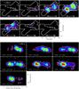 |
Fig. 21 Same as Fig. 20, but for 1-0S(1). |
| In the text | |
|
Fig. 22 Brγ velocity field derived from single-Gaussian fits to the line profile extracted from every spaxel with continuum contours (20% and 50% of the peak value) in yellow. The inset shows the Brγ velocity field on the nucleus scaled in velocity from −75 km s-1 (blue) to 75 km s-1 (red). |
| In the text | |
|
Fig. 23 Same as Fig. 16, but for Brγ. All slices with constant wavelength of the datacube were convolved with a Gaussian seeing disk with a FWHM of 0.2 arcsec. |
| In the text | |
|
Fig. 24 Same as Fig. 16, but for 1-0S(1). All slices with constant wavelength of the datacube were convolved with a Gaussian seeing disk with a FWHM of 0.15 arcsec. |
| In the text | |
|
Fig. A.1 Sky-subtracted detector image of NGC4151. The dispersion axis runs horizontally. Various electronic effects can be identified, such as bias variations in the multiplexer readout channels and electronic ghosts. The staggered arrangement of the spectra can also be seen in the inset. |
| In the text | |
Current usage metrics show cumulative count of Article Views (full-text article views including HTML views, PDF and ePub downloads, according to the available data) and Abstracts Views on Vision4Press platform.
Data correspond to usage on the plateform after 2015. The current usage metrics is available 48-96 hours after online publication and is updated daily on week days.
Initial download of the metrics may take a while.