| Issue |
A&A
Volume 549, January 2013
|
|
|---|---|---|
| Article Number | A132 | |
| Number of page(s) | 16 | |
| Section | Galactic structure, stellar clusters and populations | |
| DOI | https://doi.org/10.1051/0004-6361/201219648 | |
| Published online | 14 January 2013 | |
Local-density-driven clustered star formation
1
Astronomisches Rechen-Institut, Zentrum für Astronomie, Heidelberg
Universität,
Mönchhofstr. 12-14,
69120
Heidelberg,
Germany
2
Max-Planck-Institut für Radioastronomie,
Auf dem Hügel 69,
53121
Bonn,
Germany
3
Argelander-Institut für Astronomie, Bonn Universität,
Auf dem Hügel 71,
53121
Bonn,
Germany
e-mail: This email address is being protected from spambots. You need JavaScript enabled to view it.
Received:
22
May
2012
Accepted:
23
October
2012
Abstract
Context. A positive power-law trend between the local surface densities of molecular gas, Σgas, and young stellar objects, Σ ⋆ , in molecular clouds of the solar neighbourhood has recently been identified. How it relates to the properties of embedded clusters, in particular to the recently established radius-density relation, has so far not been investigated.
Aims. We model the development of the stellar component of molecular clumps as a function of time and initial local volume density. Our study provides a coherent framework able to explain both the molecular-cloud and embedded-cluster relations quoted above.
Methods. We associate the observed volume density gradient of molecular clumps to a density-dependent free-fall time. The molecular clump star formation history is obtained by applying a constant star formation efficiency per free-fall time, ϵff.
Results. For the volume density profiles typical of observed molecular clumps (i.e. power-law slope ≃ −1.7), our model gives a star-gas surface-density relation of the form Σ⋆ ∝ Σgas2, which agrees very well with the observations. Taking the case of a molecular clump of mass M0 ≃ 104 M⊙ and radius R ≃ 6 pc experiencing star formation during 2 Myr, we derive what star formation efficiency per free-fall time matches the normalizations of the observed and predicted (Σ ⋆ , Σgas) relations best. We find ϵff ≃ 0.1. We show that the observed growth of embedded clusters, embodied by their radius-density relation, corresponds to a surface density threshold being applied to developing star-forming regions. The consequences of our model in terms of cluster survivability after residual star-forming gas expulsion are that, owing to the locally high star formation efficiency in the inner part of star-forming regions, global star formation efficiency as low as 10% can lead to the formation of bound gas-free star clusters.
Key words: stars: formation / galaxies: star clusters: general / ISM: clouds / stars: kinematics and dynamics
© ESO, 2013
1. Introduction
Properties of star-cluster forming regions are crucial to determining how the nascent
cluster dynamically responds when the gas left unprocessed by star formation is driven out
by stellar feedback. Does the cluster survive as a bound entity, albeit depleted of a
fraction of its stars, or is it fully dispersed into the field? Pivotal properties
influencing the likelihood of cluster survival include the star formation efficiency of
cluster-forming regions and their potential well depth. The latter can be quantified through
their mass-radius relation, which several authors report to scale as
 , where
mecl and recl are the
embedded-cluster stellar mass and radius, respectively (Lada
& Lada 2003; Adams et al. 2006). We
stress that this relation only refers to the stars; i.e. mecl
does not account for the unprocessed gas.
, where
mecl and recl are the
embedded-cluster stellar mass and radius, respectively (Lada
& Lada 2003; Adams et al. 2006). We
stress that this relation only refers to the stars; i.e. mecl
does not account for the unprocessed gas.
This mass-radius relation is one of constant mean surface density, and it can stem from the method applied to measure the embedded-cluster radius and the stellar mass it contains. As pointed out by Allen et al. (2007), if the mass and radius of a cluster are defined based on a surface density threshold, they are necessarily sensitive to the adopted density cut-off. This also determines what mass fraction of the stars is hosted by the “halo” surrounding the star cluster, as opposed to the cluster itself. For a given star-forming region, the higher the surface density threshold, the smaller the cluster mass and radius, and the larger the surrounding “halo”. This renders an accurate definition of the cluster-forming region problematic.
Besides this, it is worth stressing that the dynamical response of a cluster to the residual star-forming gas expulsion depends on the cluster-forming region properties at the onset of gas expulsion. This prompts another key question when quantifying cluster-forming region properties: is an observed embedded cluster caught in the process of turning its gas into stars, or has it just reached the end point of star formation with the intra-cluster gas about to be expelled? Higuchi et al. (2009, 2010) illustrate the problem well. Their C18O mapping of 14 molecular clumps, each forming a star cluster, shows a sequence of star formation efficiencies. The highest efficiencies are found for clusters associated to C18O-emission holes, highlighting that gas dispersal has started there1. Therefore, an observed star formation efficiency is not enough to assess how the corresponding cluster will respond to gas expulsion. In Sect. 4.1.2, we suggest an alternative explanation to gas dispersal to explain the C18O-emission holes of some cluster-forming clumps.
The characterization of cluster-forming regions has made a significant leap forward thanks to the Spitzer Space Telescope. Spitzer has probed a wide spectrum of stellar densities in star-forming environments of the solar neighbourhood – from relative isolation to star clusters (although the Trapezium region of the Orion Nebula Cluster remains unresolved with that facility). Spitzer-surveys have led to a new picture, that is, star clusters are the emerging stellar peaks of wider star-forming regions (Allen et al. 2007; Evans et al. 2009; Gutermuth et al. 2011). Understanding the physics of cluster formation and the properties of star-forming regions at large are therefore now tightly entwined topics.
Gutermuth et al. (2011) identifies a positive
power-law trend between the local surface densities of molecular gas and young stellar
objects (YSOs) in eight molecular clouds located within 1 kpc of the Sun. On the average,
the relation between the local YSO surface density, ΣYSO, and the local gas
surface density, Σg, follows  , with
α ≃ 2 and the surface densities in units of
M⊙ pc-2. Their result is based on mapping
Spitzer-identified YSO spatial distributions with a nth
nearest neighbour scheme, and tracing the molecular gas by near-infrared extinction. In most
molecular clouds of the sample, the power-law scaling is affected by a large scatter
(~1 dex, see Fig. 9 in Gutermuth et al. 2011). It
is tightest in the Ophiuchus and MonR2 clouds where the power-law index α
is 1.9 and 2.7, respectively. One of the purposes of this contribution is to show how this
star formation law and the physics of cluster formation are related.
, with
α ≃ 2 and the surface densities in units of
M⊙ pc-2. Their result is based on mapping
Spitzer-identified YSO spatial distributions with a nth
nearest neighbour scheme, and tracing the molecular gas by near-infrared extinction. In most
molecular clouds of the sample, the power-law scaling is affected by a large scatter
(~1 dex, see Fig. 9 in Gutermuth et al. 2011). It
is tightest in the Ophiuchus and MonR2 clouds where the power-law index α
is 1.9 and 2.7, respectively. One of the purposes of this contribution is to show how this
star formation law and the physics of cluster formation are related.
There is increasing evidence for a bimodal cluster formation process. Da Costa et al. (2009) find that the half-light radius distribution of extragalactic old globular clusters is bimodal. Similarly, Baumgardt et al. (2010) identify two populations of globular clusters in the outer halo of our Galaxy based on the ratio of their half-mass to Jacobi radii. They suggest that this bimodality is an imprint of cluster formation, rather than a consequence of 13 Gyr of dynamical evolution in the Galactic halo (see also Elmegreen 2008). In addition, a bimodal cluster formation agrees with the finding of Pfalzner (2009) that, in the Galactic disc, star clusters younger than 20 Myr unfold along two distinct sequences in the space of cluster volume density versus cluster radius (her Fig. 2). She coins them the starburst and leaky clusters. (Maíz Apellániz 2001 identifies a similar dichotomy in the structural properties of a sample of nearby extragalactic clusters.) Pfalzner (2009) also notes that the embeddded clusters of Lada & Lada (2003) define a precursor sequence to the leaky clusters (her Fig. 4). That is, these embedded clusters seem to be the leaky-cluster progenitors, with starburst cluster precursors still to be identified.
In a follow-up study, Pfalzner (2011) shows that the
embedded-cluster sequence obeys  ,
where ρecl is the cluster mean volume density (her Fig. 2). This
is reminiscent of a relation of constant mean surface density, i.e.
,
where ρecl is the cluster mean volume density (her Fig. 2). This
is reminiscent of a relation of constant mean surface density, i.e.
 ,
as put forward by Adams et al. (2006) and Allen et al. (2007). She presents the embedded-cluster
sequence as a growth sequence, that is, clusters are still in the process of building their
stellar mass and their properties may therefore not be representative of the conditions at
gas expulsion onset. The embedded-cluster scaling
equates with
,
as put forward by Adams et al. (2006) and Allen et al. (2007). She presents the embedded-cluster
sequence as a growth sequence, that is, clusters are still in the process of building their
stellar mass and their properties may therefore not be representative of the conditions at
gas expulsion onset. The embedded-cluster scaling
equates with  . This implies
that, as the embedded-cluster (stellar) mass mecl increases with
time, so does the radius recl, while the mean volume density
ρecl decreases. In other words, in this scenario, star
formation propagates outwardly. The cluster central regions form first, and outer shells of
stars are added with time. This is an extremely appealing concept for the following reason.
The timescale relevant for star formation is the free-fall time of the star-forming gas,
τff (Elmegreen 2007;
Krumholz & Tan 2007). Since
τff scales with the gas volume density as
. This implies
that, as the embedded-cluster (stellar) mass mecl increases with
time, so does the radius recl, while the mean volume density
ρecl decreases. In other words, in this scenario, star
formation propagates outwardly. The cluster central regions form first, and outer shells of
stars are added with time. This is an extremely appealing concept for the following reason.
The timescale relevant for star formation is the free-fall time of the star-forming gas,
τff (Elmegreen 2007;
Krumholz & Tan 2007). Since
τff scales with the gas volume density as
 and
since molecular clumps have radial density gradients (Beuther
et al. 2002; Müller et al. 2002; Pirogov 2009), the gas free-fall time is shorter in the
denser inner regions of molecular clumps than in their outskirts. That is, star formation is
faster closer to the clump centre than towards the clump edge.
and
since molecular clumps have radial density gradients (Beuther
et al. 2002; Müller et al. 2002; Pirogov 2009), the gas free-fall time is shorter in the
denser inner regions of molecular clumps than in their outskirts. That is, star formation is
faster closer to the clump centre than towards the clump edge.
Here comes a subtle difference, however. Is star formation in the outer regions of a molecular clump delayed, or does star formation start at the same time all through the molecular clump, albeit at a slower rate at larger distance from the clump centre? The scenario devised by Pfalzner (2011) clearly fits the first hypothesis. In contrast, a molecular clump forming stars on a radially-varying timescale would match the second hypothesis.
Considerable efforts have been dedicated to the hydrodynamical simulations of star formation in molecular gas (e.g. Klessen et al. 1998; Bate et al. 2003; Bonnell et al. 2008). These simulations are computationally expensive and hence limited in terms of the modelled gas mass (e.g. 104 M⊙, Bonnell et al. 2008). Parametric semi-analytical studies remain therefore useful, especially to browse the parameter space extensively.
In this contribution, we build on the concept of star formation efficiency per free-fall
time originally introduced by Krumholz & McKee
(2005), namely, the fraction of an object’s gaseous mass that is processed into
stars over one free-fall time at the mean density of the object2. We generalize their approach by defining a local free-fall time. That is, we
present a new model for star-forming regions which hinges on the radially-varying free-fall
time of molecular clumps. We show how it provides an elegant and coherent picture that
accounts for both the local3 star formation law
 recenly
highlighted by Gutermuth et al. (2011) and the growth
sequence of embedded clusters postulated by Pfalzner
(2011).
recenly
highlighted by Gutermuth et al. (2011) and the growth
sequence of embedded clusters postulated by Pfalzner
(2011).
Our paper is organized as follows. In Sect. 2, we present the model and show how it straightforwardly explains the scaling law of Gutermuth et al. (2011). In Sect. 3, we fold the model with a surface density threshold. This equates with accounting for a contaminating stellar background against which the star-forming region is projected and observed. We deduce the corresponding recl-ρecl relation, where recl and ρecl are the radius and mean volume density of the part of the star-forming region that emerges above the stellar background. We find the predicted recl − ρecl relation to be in good agreement with the embedded-cluster sequence of Pfalzner (2011). Section 4 gives an overview of the model consequences in the framework of cluster gas expulsion. Finally, we outline some future directions in Sect. 5 and present our conclusions in Sect. 6.
2. Free-fall time-driven star formation
We start by studying how a spherical gas clump with a radial density gradient builds its stellar component as a function of time and space, under the assumption of a constant star formation efficiency per free-fall time, ϵff. Because of the density gradient, the free-fall time must be defined locally, i.e. τff(r), and is an increasing function of the distance r from the clump centre. Consequently, star formation proceeds more quickly in the clump’s central regions than in its outskirts. This leads to a density profile for the stellar component that is steeper than the initial density profile of the clump.
Prior to going into detailed numerical simulations, we present a simple analytical approximation which allows the relevant physics to be grasped.
2.1. Analytical insights
Assuming spherical symmetry, the volume density profile,
ρ0(r), of a molecular clump of mass
M0, radius R0, and density
index p0, obeys  (1)where r
is the distance from the clump centre. The subscript “0” refers to the gas properties
prior to star formation (i.e. at t = 0: the clump is made of gas alone).
The factor kρ,0 comes from integrating the
density profile over the clump volume, i.e.
(1)where r
is the distance from the clump centre. The subscript “0” refers to the gas properties
prior to star formation (i.e. at t = 0: the clump is made of gas alone).
The factor kρ,0 comes from integrating the
density profile over the clump volume, i.e.  . The density index of
star-forming molecular clumps is observed to range from ≃ 1.5 to ≃ 2.0. We therefore
assume 1.5 ≲ p0 ≲ 2.0 (Beuther
et al. 2002; Müller et al. 2002)4.
. The density index of
star-forming molecular clumps is observed to range from ≃ 1.5 to ≃ 2.0. We therefore
assume 1.5 ≲ p0 ≲ 2.0 (Beuther
et al. 2002; Müller et al. 2002)4.
In this model, we assume that star-forming molecular clumps neither experience significant outflows or inflows, nor do they contract or expand during star formation. We also neglect the potential migration of YSOs after their formation. As a result of these assumptions, at any time t after the onset of star formation, the clump total mass (gas + stars) is preserved, i.e. M ⋆ (t) + Mg(t) = M0, as well as the clump radius R0 and the spatial distribution of the clump mass, i.e. ρ ⋆ (t,r) + ρg(t,r) = ρ0(r). The subscripts “g” and “ ⋆ ” refer to the properties of, respectively, the unprocessed gas and stellar component at any time t > 0. As an example, we write ρg and ρ0 for the current and initial gas volume densities. Finally, we consider that the star formation efficiency per free-fall time, ϵff, is constant. In this class of model, star formation takes place over the whole clump, albeit at a slower rate in the outskirts than in the centre. The limiting radii of the clump and of its stellar component are therefore equal: R0 = R ⋆ . In what follows, we refer to both radii as R.
We now consider that, at any time t, a fraction
ϵff of the gas mass at radius r is turned
into stars each local free-fall time. Because of the volume density gradient of the
molecular clump, star formation proceeds more quickly in its centre than in its outskirts.
As a result, the volume density profile of the stellar component built by the clump,
ρ ⋆ (t,r), is steeper than
ρ0(r). We insist that this stems from the
shorter free-fall time at smaller radius, not from a higher
ϵff in the clump centre. The free-fall time of the gas at
radius r and time t obeys  (2)with G
the gravitational constant and ρg(t,r) the
volume density profile of the unprocessed gas at time t.
(2)with G
the gravitational constant and ρg(t,r) the
volume density profile of the unprocessed gas at time t.
We then assume that the volume density profile of the stellar component is a power law,
too, with a constant density index q:  (3)As we shall see
from the numerical modelling, this is a realistic approximation (see top and middle panels
of Fig. 1 and top panel of Fig. 5). In Eq. (3),
M ⋆ (t) is the total
stellar mass contained by the clump at time t. As previously, the factor
kρ, ⋆ stems from
integrating the density profile over the entire clump volume, i.e.
(3)As we shall see
from the numerical modelling, this is a realistic approximation (see top and middle panels
of Fig. 1 and top panel of Fig. 5). In Eq. (3),
M ⋆ (t) is the total
stellar mass contained by the clump at time t. As previously, the factor
kρ, ⋆ stems from
integrating the density profile over the entire clump volume, i.e.
 .
.
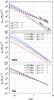 |
Fig. 1 Top panel: initial gas volume density profiles (filled symbols) and their associated steeper stellar density profiles (open symbols). The latter are obtained from the numerical or analytical model one million years after star formation onset, i.e. t = 1 Myr, for three distinct p0 density indices (see key). The spherical molecular clump has a mass M0 ≃ 104 M⊙, a radius R ≃ 6 pc, and the star formation efficiency per free-fall time is ϵff = 0.1. Middle panel: stellar density profiles from the numerical model (lines with open symbols) for the times t and density indices p0 quoted in the key. Each symbol-free line is the corresponding analytical upper limit (Eq. (8)). Bottom panel: time evolution of the gas volume density profile for p0 = 1.7. The star-formation-driven depletion of the gas in the central region of the molecular clump – where the free-fall time is the shortest – is clearly highlighted. The symbol-free dotted line over the range 0.2−1 pc has a slope of −1.3, i.e. shallower than the initial slope −1.7. |
Because the stellar component is steeper than the initial gas density profile, we have
q > p0. How much
steeper is q compared to p0? We assume for a
moment that, at any time t and radius r, the gas mass
keeps dominating the stellar mass. That is to say, in
ρ ⋆ (t,r) + ρg(t,r) = ρ0(r),
we assume
ρ ⋆ (t,r) ≪ ρg(t,r),
which leads to
ρg(t,r) ≃ ρ0(r),
and the gas density profile does not evolve significantly. Therefore, the local free-fall
time (Eq. (2)) is approximately constant,
too:  (4)We now consider a
shell of thickness dr at a distance r from the clump
centre and of initial gas mass
dm0(r) = 4πr2ρ0(r)dr.
Under the assumption of a constant free-fall time (Eq. (4)), the stellar mass formed by this shell at time t,
dm ⋆ (t,r), follows from
(4)We now consider a
shell of thickness dr at a distance r from the clump
centre and of initial gas mass
dm0(r) = 4πr2ρ0(r)dr.
Under the assumption of a constant free-fall time (Eq. (4)), the stellar mass formed by this shell at time t,
dm ⋆ (t,r), follows from
 (5)where
t/τff(t = 0,r)
is the number of free-fall times elapsed since star formation started. The right-hand side
of Eq. (5) defines an upper limit to the
actual mass in YSOs in the shell at time t, for two reasons. Firstly, as
time goes by, the star formation efficiency per free-fall time is applied to an ever lower
gas mass, i.e.
dmg(t,r) < dm0(r).
Secondly, the steady decrease in the gas mass lengthens the local free-fall time; i.e. we
have
τff(t,r) ≥ τff(t = 0,r)
instead of Eq. (4). Equation (5) can be rewritten as
(5)where
t/τff(t = 0,r)
is the number of free-fall times elapsed since star formation started. The right-hand side
of Eq. (5) defines an upper limit to the
actual mass in YSOs in the shell at time t, for two reasons. Firstly, as
time goes by, the star formation efficiency per free-fall time is applied to an ever lower
gas mass, i.e.
dmg(t,r) < dm0(r).
Secondly, the steady decrease in the gas mass lengthens the local free-fall time; i.e. we
have
τff(t,r) ≥ τff(t = 0,r)
instead of Eq. (4). Equation (5) can be rewritten as 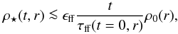 (6)Combining Eqs. (2) and (6) leads to
 ![Mathematical equation: \begin{equation} \rhost(t,r) \la \sqrt{\frac{32 G}{3 \pi}} \eff t \left[\rho_0(r)\right]^{3/2}. \label{eq:uplim0} \end{equation}](/articles/aa/full_html/2013/01/aa19648-12/aa19648-12-eq84.png) (7)Introducing
Eq. (1) then gives
(7)Introducing
Eq. (1) then gives 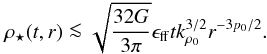 (8)The right-hand side
of Eq. (8) is shown as the symbol-free
lines in the middle panel of Fig. 1. The exact
solutions, which account for the time variations in the gas mass and in the local
free-fall time, are obtained in Sect. 2.2 (numerical
model) or in Sect. 2.3 (analytical model). The panel
highlights clearly that the analytical approximation provides an upper limit to the actual
stellar density profile. We assume
M0 ≃ 104 M⊙,
R ≃ 6 pc and ϵff = 0.1 (values discussed
in Sect. 2.2). Star-formation durations
t and density indices p0 are given in the
key.
(8)The right-hand side
of Eq. (8) is shown as the symbol-free
lines in the middle panel of Fig. 1. The exact
solutions, which account for the time variations in the gas mass and in the local
free-fall time, are obtained in Sect. 2.2 (numerical
model) or in Sect. 2.3 (analytical model). The panel
highlights clearly that the analytical approximation provides an upper limit to the actual
stellar density profile. We assume
M0 ≃ 104 M⊙,
R ≃ 6 pc and ϵff = 0.1 (values discussed
in Sect. 2.2). Star-formation durations
t and density indices p0 are given in the
key.
The right-hand side of Eq. (8) works best as an analytical approximation for ρ ⋆ (t,r) in the clump outskirts where the local free-fall time is the longest. That is, the hypothesis ρg(t,r) ≃ ρ0(r) remains valid for the time span of our simulations (up to 2.5 Myr), and Eq. (8) can be seen as an equality (rather than an upper limit). In the inner regions, however, the shorter free-fall time implies a gas depletion quicker than in the outskirts. This eventually results in ρg(t,r) < ρ0(r), τff(t,r) > τff(t = 0,r) (star formation slows down), and the right-hand side of Eq. (8) gives a firm upper limit. This differential behaviour between the inner and outer regions means that the actual stellar density profile is shallower than given by the right-hand side of Eq. (8) (compare the symbol-free lines and the lines with open symbols in the middle panel of Fig. 1, especially for the p0 = 1.9 model). In other words, the stellar density profile is steeper than the initial gas density profile (Eq. (7)) by at most a factor 1.5; e.g., an initial gas density index p0 = 1.7 gives rise to a star density index q ≲ 3p0/2 = 2.55.
We now have to convert the volume density profiles into (projected) surface density
profiles, since observer-retrieved quantities are surface densities. For power-law volume
density profiles, the surface density profiles are shallower than their volume
counterparts by 1 dex. Therefore, the surface density profiles of the gas, initially and
at time t, and of the stars obey 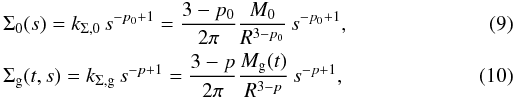 and
and
 (11)respectively. The
factors
kΣ,(0,g, ⋆ )
come from integrating the surface densities over the whole molecular clump surface:
(11)respectively. The
factors
kΣ,(0,g, ⋆ )
come from integrating the surface densities over the whole molecular clump surface:
 , where s
is the projected distance from the clump centre. In other words, s is a
two-dimensional distance on the plane of the sky, while r is a
three-dimensional distance.
, where s
is the projected distance from the clump centre. In other words, s is a
two-dimensional distance on the plane of the sky, while r is a
three-dimensional distance.
With the surface density profiles (Eqs. (9)–(11)) derived above and an
estimate of the star density index
(q ≲ 3p0/2), we are now
ready to infer the local star formation law
Σ ⋆ (t,s) ∝ Σg(t,s)α
predicted by the analytical approximation. Eliminating the two-dimensional distance
s between Eqs. (10)
and (11), we obtain ![Mathematical equation: \begin{equation} \Sigst(t,s) = \frac{(3-q)M\st(t)}{[(3-p)M_{\rm g}(t)]^{\frac{q-1}{p-1}}} (2\pi R^2)^{\frac{q-p}{p-1}} \left( \Sigma_{\rm g}(t,s) \right)^{\frac{q-1}{p-1}}\cdot \label{eq:sfl_mod0} \end{equation}](/articles/aa/full_html/2013/01/aa19648-12/aa19648-12-eq99.png) (12)Under our assumption that
the gas mass dominates the stellar mass throughout the clump,
Σ0(s) = Σg(t,s) + Σ ⋆ (t,s) ≃ Σg(t,s)
and we substitute Σ0(s) to Σg(t,s)
in Eq. (12). This leads to
(12)Under our assumption that
the gas mass dominates the stellar mass throughout the clump,
Σ0(s) = Σg(t,s) + Σ ⋆ (t,s) ≃ Σg(t,s)
and we substitute Σ0(s) to Σg(t,s)
in Eq. (12). This leads to ![Mathematical equation: \begin{equation} \Sigst(t,s) = \frac{(3-q)M\st(t)}{[(3-p_0)M_0]^{\frac{q-1}{p_0-1}}} (2\pi R^2)^{\frac{q-p_0}{p_0-1}} \left( \Sigma_0(s) \right)^{\frac{q-1}{p_0-1}}\cdot \label{eq:sfl_mod} \end{equation}](/articles/aa/full_html/2013/01/aa19648-12/aa19648-12-eq103.png) (13)Considering the index
α of this relation
(13)Considering the index
α of this relation  (14)it immediately
appears that a density profile steeper for the stellar component than for the gas (i.e.
q > p0) is
conducive to α > 1, as found by Gutermuth et al. (2011). Were the density indices for
the gas and stars identical (i.e. q = p0,
equivalent to no radial variations of the local star formation efficiency; see also
Sect. 4.1.2), α would be unity.
There is therefore a causal link between (i) the slope of the relation between the gas and
YSO surface densities (Eq. (13)), and
(ii) how much steeper the volume density profile of the stars is compared to that of the
gas (Eq. (7)). Adopting
p0 = 1.7 and
q ≲ 3p0/2 = 2.55 leads
to α ≲ 2.2, in fair agreement with the mean power-law trend observed by
Gutermuth et al. (2011). This quantitative result
provides us with a strong incentive to refine the
(Σ ⋆ ,Σg) relation by means of
numerical simulations.
(14)it immediately
appears that a density profile steeper for the stellar component than for the gas (i.e.
q > p0) is
conducive to α > 1, as found by Gutermuth et al. (2011). Were the density indices for
the gas and stars identical (i.e. q = p0,
equivalent to no radial variations of the local star formation efficiency; see also
Sect. 4.1.2), α would be unity.
There is therefore a causal link between (i) the slope of the relation between the gas and
YSO surface densities (Eq. (13)), and
(ii) how much steeper the volume density profile of the stars is compared to that of the
gas (Eq. (7)). Adopting
p0 = 1.7 and
q ≲ 3p0/2 = 2.55 leads
to α ≲ 2.2, in fair agreement with the mean power-law trend observed by
Gutermuth et al. (2011). This quantitative result
provides us with a strong incentive to refine the
(Σ ⋆ ,Σg) relation by means of
numerical simulations.
2.2. Numerical model
In the numerical model, we discretize the spherical molecular clump into successive
shells defined by their three-dimensional radius r, local volume density
ρg(t,r) and local free-fall time
τff(t,r) at time t. Every
instantaneous local free-fall time, a fraction ϵff of the gas
mass is removed and added to the stellar content:  \arraycolsep1.75ptThe
local gas free-fall time (Eq. (2)) is then
updated. As the gas gets depleted, star formation slows down, an effect unaccounted for in
the analytical approximation of Sect. 2.1.
\arraycolsep1.75ptThe
local gas free-fall time (Eq. (2)) is then
updated. As the gas gets depleted, star formation slows down, an effect unaccounted for in
the analytical approximation of Sect. 2.1.
The numerical results are shown in Fig. 1, for the
case of a spherical gas clump of mass
M0 = 104 M⊙,
radius R = 6 pc and star formation efficiency per free-fall time
ϵff = 0.1. Our choice of the mass and radius stems from
inspecting the extinction map of the MonR2 molecular cloud and its spatial distribution of
Spitzer-identified YSOs (Gutermuth
et al. 2011, their Fig. 1). We focus on the highest concentration of YSOs (at a
right ascension of ≃ 06h08m and declination of
≃ −6°24′) for which we adopt a radius R = 6 pc
so as to include the lowest YSO surface densities. We adopt
M0 = 104 M⊙ as a
rough estimate of the initial gas mass within R = 6 pc given that this
region represents a significant fraction of the MonR2 cloud whose total mass is
25 800 M⊙ (Table 1 in Gutermuth et al. 2011). We plan to map our model onto detailed observational
data in the near future. In the mean time, we stress that the estimate of
ϵff we adopt to make our model match the averaged local star
formation law,  , depends on the
chosen values for M0 and R (see below and top
panel of Fig. 3).
, depends on the
chosen values for M0 and R (see below and top
panel of Fig. 3).
As for the upper limit on the time t elapsed since the onset of star formation, we note that Gutermuth et al. (2011) study encompasses mostly Class I protostars and Class II pre-main-sequence stars. Given that the respective average lifetimes of the Class I and Class II phases are ≃ 0.5 Myr and ≃ 2 Myr (Evans et al. 2009), we adopt 2.5 Myr as the time span of our simulations.
The top panel of Fig. 1 illustrates the initial volume density profile of the gas for different density indices: p0 = 1.5,1.7 and 1.9. Also depicted are the volume density profiles of the built-in stellar component at t = 1 Myr, thereby highlighting the steepening of the stellar density profile compared to the initial spatial distribution of the gas. The gas-to-star steepening corresponds to a local star formation efficiency higher in the clump central region than in its outskirts. We come back to this point in Sect. 4.1.2. The middle panel shows the stellar density profiles for the gas density indices p0 and times t quoted in the key. Each profile is shown along with its upper limit predicted by Eq. (8). The difference between the analytical approximation and the numerical model is stronger when the free-fall time is short, e.g. in the clump inner regions, especially for a steep density profile (high p0). The difference also gets greater for longer star-formation durations t. Nevertheless, the comparison between both demonstrates the excellence of Eq. (8) in providing a back-of-the-envelope estimate of the stellar density profile. The bottom panel of Fig. 1 depicts the time evolution of the gas density profile when p0 = 1.7. Its flattening in the clump centre contrasts markedly with the absence of evolution at the clump edge where the initial free-fall time is the longest. The instantaneous gas density index, p, thus becomes smaller as t increases (i.e. the gas density profile becomes shallower).
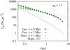 |
Fig. 2 Surface density profiles from the numerical model. Lines with circles from top to bottom: the molecular clump gas initially, the unprocessed gas and the stellar component at t = 1 Myr (see key). The molecular clump is the same as in Fig. 1, and the initial gas density index is p0 = 1.7. The solid symbol-free line depicts a slope of −0.7 which is the slope expected for the initial surface density profile of the gas when p0 = 1.7. We note that in the clump outskirts, the actual surface density profile becomes increasingly steeper than the power-law approximation. |
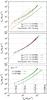 |
Fig. 3 Local surface density of YSOs, Σ ⋆ , in dependence on the local surface density of the unprocessed/observed gas, Σg. Top panel: models for a molecular clump of mass M0 = 104 M⊙, radius R = 6 pc, density index p0 = 1.7, a star formation efficiency per free-fall time ϵff = 0.1 and the times t quoted in the key. The dotted (black) line depicts the average star-formation law inferred by Gutermuth et al. (2011). The orange and brown polygons illustrate the associated scatter observed for the MonR2 and Ophiuchus molecular clouds, where it is the smallest. Middle panel: models for a time t = 2 Myr and three distinct density indices of the molecular clump, p0 = 1.5, 1.7, and 1.9. The normalization of the model hardly depends on p0. Bottom panel: same as top panel but completed with the time evolution of the gas and YSO surface densities at four projected distances s from the clump centre (s-labelled dotted black lines). |
2.3. Analytical solution
The actual time evolution of the star and gas density profiles can also be obtained
analytically. Equations (15), (16) correspond to separable first-order
differential equations. Using Eq. (2), they
can be rewritten as  and
their solutions are
and
their solutions are 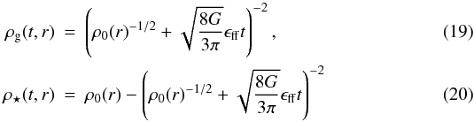 where
the clump density profile ρ0(r) is given by
Eq. (1). Equations (19) and (20) correspond, respectively, to the numerical solutions shown in the
bottom panel of Fig. 1 and in the top and middle
panels of Fig. 1.
where
the clump density profile ρ0(r) is given by
Eq. (1). Equations (19) and (20) correspond, respectively, to the numerical solutions shown in the
bottom panel of Fig. 1 and in the top and middle
panels of Fig. 1.
Before going any further, we recall that our model builds on the local free-fall time;
that is, it quantifies the local (at the radius r) collapse of the gas.
The global collapse of the star-forming molecular clump (i.e. its collapse to its centre)
may also be relevant to its evolution. The free-fall time to the clump centre depends on
the mean volume density enclosed within the radius r,
 ,
and may therefore be shorter than the local free-fall time, especially for steep density
profiles (e.g. the outskirts of some molecular clumps; see Fig. 2 in Beuther et al. 2002). That is to say, were the clump evolution driven
only by gravity, the gas would collapse to the clump centre faster than it does locally.
The significance of the global collapse with respect to the local one therefore depends on
how much the gas is supported by the combined effects of turbulence, magnetic fields, etc.
A study of that aspect is beyond the scope of the present paper, and we assume for now
that the star-formation history of the molecular clump is solely driven by the local
collapse of its gas. As already quoted in Sect. 2.1,
once the YSOs have formed at radius r through the gas local collapse, we
neglect their potential migration towards other regions of the molecular clump. The actual
behaviour of newly-formed stars depends on their velocities at formation. If their initial
velocity is sub-virial, once decoupled from the gas, they will fall to the cluster centre
where they will revirialize (see e.g. Girichidis et al.
2012a).
,
and may therefore be shorter than the local free-fall time, especially for steep density
profiles (e.g. the outskirts of some molecular clumps; see Fig. 2 in Beuther et al. 2002). That is to say, were the clump evolution driven
only by gravity, the gas would collapse to the clump centre faster than it does locally.
The significance of the global collapse with respect to the local one therefore depends on
how much the gas is supported by the combined effects of turbulence, magnetic fields, etc.
A study of that aspect is beyond the scope of the present paper, and we assume for now
that the star-formation history of the molecular clump is solely driven by the local
collapse of its gas. As already quoted in Sect. 2.1,
once the YSOs have formed at radius r through the gas local collapse, we
neglect their potential migration towards other regions of the molecular clump. The actual
behaviour of newly-formed stars depends on their velocities at formation. If their initial
velocity is sub-virial, once decoupled from the gas, they will fall to the cluster centre
where they will revirialize (see e.g. Girichidis et al.
2012a).
2.4. Surface densities and the local star formation law
Following the analytical aproximations obtained in Sect. 2.1 (Eqs. (10) (11)), we now derive the numerical solutions for the gas and star surface density profiles. To derive the exact surface density profiles, we build on Eq. (6) of Parmentier et al. (2011), which integrates a power-law volume density profile into the projected mass enclosed within an aperture of radius sap (see also their Fig. 3). This provides straightforwardly the projected mass within a circular corona of radius sap and thickness dsap. Gas and star surface density profiles are shown in Fig. 2 for the same molecular clump as previously, p0 = 1.7 and the times t quoted in the key. The local star-formation law predicted by our numerical model can now be derived and compared with the scaling observed by Gutermuth et al. (2011).
Figure 3 depicts the local surface density of YSOs,
Σ ⋆ , in dependence on the local surface density of the
observed/unprocessed gas, Σg. Both surface densities are in units of
M⊙ pc-2. The scaling law of Gutermuth et al. (2011), i.e.
 , is shown in the
top and middle panels. The top panel shows the numerical model for
p0 = 1.7 at t = 0.5 Myr and
t = 2.0 Myr. The agreement between the model at
t = 2.0 Myr and the mean observed scaling is excellent, both in terms of
slope and normalization. However, this agreement is parameter-dependent as a molecular
clump more massive (hence denser), or a longer time span, or a higher star formation
efficiency per free-fall time, all would shift the normalization upwards. The
t = 2 Myr model bends upwards at high surface density. This is due to
the flattening of the gas density profile in the clump centre; that is, p
decreases which in turn increases the index α of the local star formation
law (Eq. (14); see also bottom panel of
Fig. 3).
, is shown in the
top and middle panels. The top panel shows the numerical model for
p0 = 1.7 at t = 0.5 Myr and
t = 2.0 Myr. The agreement between the model at
t = 2.0 Myr and the mean observed scaling is excellent, both in terms of
slope and normalization. However, this agreement is parameter-dependent as a molecular
clump more massive (hence denser), or a longer time span, or a higher star formation
efficiency per free-fall time, all would shift the normalization upwards. The
t = 2 Myr model bends upwards at high surface density. This is due to
the flattening of the gas density profile in the clump centre; that is, p
decreases which in turn increases the index α of the local star formation
law (Eq. (14); see also bottom panel of
Fig. 3).
It is worth keeping in mind that  defines an average
relation. The YSO-vs.-gas relation observed for each molecular cloud exhibits a
considerable scatter (see the panels of Fig. 9 in Gutermuth et al. 2011). This is because a molecular cloud consists of several
molecular clumps, each with its own mass, radius, density index, and duration of the
star-formation process. Therefore, a molecular cloud combines several correlations, each
with its own normalization, corresponding to the several molecular clumps it contains.
This leads to a trend in the observed
(Σg,Σ ⋆ ) space, rather than
the one-to-one relation predicted for a single molecular clump and depicted in Fig. 3. Other reasons for the spread in the observed
(Σg,Σ ⋆ ) relation include YSO
migration and gas dispersal via stellar feedback processes (Gutermuth et al. 2011), and non-spherical molecular clumps. Gutermuth et al. (2011) note that the scatter is
smallest in the MonR2 and Ophiuchus molecular clouds, which they represent as the green
and blue parallelograms in their Fig. 9. They are reproduced in the top panel of our
Fig. 3.
defines an average
relation. The YSO-vs.-gas relation observed for each molecular cloud exhibits a
considerable scatter (see the panels of Fig. 9 in Gutermuth et al. 2011). This is because a molecular cloud consists of several
molecular clumps, each with its own mass, radius, density index, and duration of the
star-formation process. Therefore, a molecular cloud combines several correlations, each
with its own normalization, corresponding to the several molecular clumps it contains.
This leads to a trend in the observed
(Σg,Σ ⋆ ) space, rather than
the one-to-one relation predicted for a single molecular clump and depicted in Fig. 3. Other reasons for the spread in the observed
(Σg,Σ ⋆ ) relation include YSO
migration and gas dispersal via stellar feedback processes (Gutermuth et al. 2011), and non-spherical molecular clumps. Gutermuth et al. (2011) note that the scatter is
smallest in the MonR2 and Ophiuchus molecular clouds, which they represent as the green
and blue parallelograms in their Fig. 9. They are reproduced in the top panel of our
Fig. 3.
The middle panel of Fig. 3 illustrates how the model responds to varying the gas density index p0. For steeper profiles, the clump inner regions become denser at the expense of the outskirts. This stretches the model towards both lower and higher surface densities, although the normalization is hardly affected.
The bottom panel completes the top panel with the time evolution of the gas and star surface densities at four projected distances s from the clump centre (black dotted lines: central regions are to the right, outskirts are to the left). As long as only a few per cent of the gas has been turned into stars, a track evolves vertically because the gas surface density does not decrease significantly. Following its vertical leg, however, the track bends leftwards, thereby embodying the combined stellar mass increase and gas mass decrease. We note that a similar plot is provided in Fig. 13 of Gutermuth et al. (2011). They assume a star formation law where the star formation rate per unit area shows a power-law dependence on the gas column density. It thus differs from our model, which builds on the time evolution of volume densities.
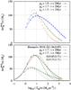 |
Fig. 4 Top panel: distribution of stellar surface densities predicted by our model for a clump of mass M0 ≃ 104 M⊙, radius R ≃ 6 pc, and star formation efficiency per free-fall time ϵff = 0.1 (clump density index p0 and time t since star formation onset are given in the key). Bottom panel: two p0 = 1.7 models are shown at time t = 1 Myr and t = 2 Myr for the same molecular clump as above (lines with open symbols). The dotted and dash-dotted (black) lines depict two Gaussians fitting their low-density regime. The solid (red) line is the Gaussian given by Bressert et al. (2010) to describe the observed local surface density distribution of YSOs in the solar neighbourhood. Mean and standard deviation of all three Gaussians are given in brackets. |
2.5. Distribution of YSO surface densities
Bressert et al. (2010) recently obtained the distribution of local surface densities of Spitzer-detected YSOs in star-forming regions of the solar neighbourhood (distance smaller than 500 pc). Their observed distribution is approximated well by a Gaussian function with a peak at ≃22 YSOs pc-2 and a standard deviation of 0.85 in log 10ΣYSOs (see their Fig. 1). A fully consistent comparison with the result of Bressert et al. (2010) still requires our model to be extended to entire molecular clouds (i.e. to accumulate many molecular clumps) since their observed distribution encompasses a dozen local star-forming regions. It is nevertheless interesting to see what stellar surface density distribution our model predicts at its current stage of development.
Building on the stellar surface density profiles derived in Sect. 2.4, Fig. 4 shows the distribution
of the logarithmic stellar surface densities, i.e., the projected mass of stars enclosed
within an annulus of radius s, d , as a function of the annulus
logarithmic surface density,
log 10(Σ ⋆ (t,s)). Units are
M⊙ and M⊙ pc-2.
The mass, radius, and star formation efficiency per free-fall time of the molecular clump
are as previously. The clump density indices p0 and times
t of the presented models are given in the key. In the bottom panel,
two models are depicted for p0 = 1.7:
t = 1 Myr and t = 2 Myr. The low surface-density regime
of each model is fitted by a Gaussian, with mean
log 10Σ ⋆ = 0.55 (t = 1 Myr)
and log 10Σ ⋆ = 0.85 (t = 2 Myr),
and a standard deviation of 0.71. They illustrate the growth of the stellar mass and
stellar surface density as time goes by. All models are bell-shaped, with wider
distributions for steeper density profiles, as expected. This suggests that the shape of
the observed distribution could be used as a probe into the density profile of star
cluster ’s parent clumps.
, as a function of the annulus
logarithmic surface density,
log 10(Σ ⋆ (t,s)). Units are
M⊙ and M⊙ pc-2.
The mass, radius, and star formation efficiency per free-fall time of the molecular clump
are as previously. The clump density indices p0 and times
t of the presented models are given in the key. In the bottom panel,
two models are depicted for p0 = 1.7:
t = 1 Myr and t = 2 Myr. The low surface-density regime
of each model is fitted by a Gaussian, with mean
log 10Σ ⋆ = 0.55 (t = 1 Myr)
and log 10Σ ⋆ = 0.85 (t = 2 Myr),
and a standard deviation of 0.71. They illustrate the growth of the stellar mass and
stellar surface density as time goes by. All models are bell-shaped, with wider
distributions for steeper density profiles, as expected. This suggests that the shape of
the observed distribution could be used as a probe into the density profile of star
cluster ’s parent clumps.
The Gaussian with which Bressert et al. (2010) describe their data is shown in the bottom panel. Assuming a mean stellar mass of 0.5 M⊙ per YSO, the surface density at their peak (≃22 YSOs pc-2) equals log 10Σ ⋆ = 1.04. Their standard deviation is 0.85 and our normalization is arbitrary. At t = 2 Myr, our p0 = 1.7 model is in good agreement with the distribution observed in the solar neighbourhood. In particular, the observed distribution agrees with our model prediction better than with the surface density distribution of sink particles of the hydrodynamics simulations of Bonnell et al. (2008) (see Fig. 2 in Kruijssen et al. 2012). It remains to be seen how including heavily crowded regions in the Bressert et al. (2010) sample would affect the comparison. Access to high-surface density regions (e.g. the core of the Orion Nebula Cluster) – which Spitzer fails to resolve and which therefore affects the high-density tail of the observed distribution – would actually allow us to test our model more extensively. Finally, we emphasize that the observation of a smooth distribution in log 10Σ ⋆ alone does not allow one to conclude that star formation is not made of multiple discrete modes (Pfalzner et al. 2012). For a set of low-mass, gas-poor clusters, Gieles et al. (2012) propose that the surface density at the peak of the observed distribution is driven by the degree of early cluster expansion.
In this section, we have developed a star-forming region model building on a constant
star formation efficiency per free-fall time in a spherical molecular clump with a radial
volume density profile
ρ0 ∝ r−p0.
When p0 ≃ 1.7 as observed, the model predicts a local
star-formation law  with
α ≃ 2. In the next section, we combine the model to a surface density
threshold imposed by the stellar background against which the star-forming region is seen
projected. We demonstrate that this leads to the time sequence for embedded-cluster
development recently proposed by Pfalzner (2011).
with
α ≃ 2. In the next section, we combine the model to a surface density
threshold imposed by the stellar background against which the star-forming region is seen
projected. We demonstrate that this leads to the time sequence for embedded-cluster
development recently proposed by Pfalzner (2011).
3. The observed growth sequence of embedded clusters
At first glance, the model presented in Sect. 2
departs from the scenario proposed by Pfalzner
(2011). In the scenario she devised based on the data of Lada & Lada (2003), an embedded cluster grows outward, with outer
shells of stars added with time. That is, star formation is delayed in the outer regions
compared to the inner ones. In contrast, in the present model, star formation proceeds all
through the molecular clump albeit at a slower rate in the outskirts than in the centre. As
quoted in Sect. 1, however, the relation inferred by
Pfalzner (2011) between the radius and the mean
volume density of embedded clusters, i.e. ,
is reminiscent of one of constant mean surface density, i.e.
.
This suggests that the data of Lada & Lada
(2003) are limited by surface density. Therefore, prior to comparing our results to
the growth sequence of Pfalzner (2011), we include
this observational bias in our model. Allen et al.
(2007) make a similar point.
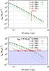 |
Fig. 5 Top panel: time evolution of the volume density profile of the stellar component for the model of Sect. 2.2: M0 = 104 M⊙, R = 6 pc, ϵff = 0.1 along with p0 = 1.7. Model time spans t are given in the key. Bottom panel: time evolution of the corresponding surface density profiles superimposed with the surface density limit, Σbck, imposed by the stellar background against which the star-forming region is projected (Carpenter et al. 2000). The shaded area shows how the surface density threshold conceals the “wings” of the stellar component, leading to observed radii (red diamonds) smaller than the actual one, i.e. sbck < R. |
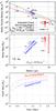 |
Fig. 6 Top panel: mean volume density in dependence of radius for (i) the whole stellar component (vertical sequence of red circles at R = 6 pc); and (ii) the associated embedded cluster (decreasing sequence of blue circles on the left). The open circle size scales with the logarithm of the stellar mass. The embedded cluster refers to the part of the star-forming region seen above the stellar background against which it is seen projected (Σbck = 40 M⊙ pc-2, solid red line). As a result of the applied surface density cut-off, the predicted embedded-cluster sequence has a constant mean surface density. Also, it does not differ much from the observed embedded-cluster sequence defined by Pfalzner (2011) (dashed green line; see text for details). The times and stellar masses are given along the plotted sequences. Middle panel: mass in stars against radius, for the whole star-forming region (red vertical track to the right) and for the developing embedded cluster (blue track to the left). Quoted to the left of the sequences are the times elapsed since the onset of star-formation (in Myr). Bottom panel: same as the middle panel but for the mass-vs-time space. |
The top and bottom panels of Fig. 5 show the rising with time of the volume- and surface-density profiles of the stellar component for the model of Sect. 2 (M0 = 104 M⊙, R = 6 pc, ϵff = 0.1) with a density index p0 = 1.7. The bottom panel also includes the surface density cut-off of Carpenter et al. (2000): Σbck = 40 M⊙ pc-2. The shaded area illustrates the surface density regime with Σ ⋆ < Σbck. We note that the embedded clusters of Lada & Lada (2003) are spread over distances from the Sun ranging from ≃100 pc to 2.4 kpc. Each cluster therefore has its own limiting background surface density. Since these are unknown, we resort to the single value of Σbck quoted above. It should be considered as a mean value used for illustrative purposes. The surface density threshold Σbck = 40 M⊙ pc-2 follows closely the embedded-cluster track defined by Pfalzner (2011, her Fig. 2). We will come back to this point in Fig. 6.
The surface density limit imposed by the stellar background conceals the “wings” of the stellar component, whose observed limiting radius is therefore smaller than the actual one, that is, sbck < R. These observed radii, sbck, are depicted in the bottom panel of Fig. 5. They define an outward time sequence, in agreement with Pfalzner (2011). In other words, while the whole stellar component follows a vertical evolution, i.e. the density increases at fixed radius, the fraction of it denser than the stellar background mimics a horizontal evolution, i.e. the observed limiting radius increases with time. In what follows, we refer the part of the stellar component whose surface density is higher than that of the background as the embedded-cluster (unshaded area in bottom panel of Fig. 5: Σ(s) > Σbck when s < sbck). That is, sbck = recl with recl the embedded-cluster radius. We define the embedded-cluster mass, mecl, as the stellar mass enclosed within the three-dimensional radius recl.
For each time step, we obtain the radius and mass of the embedded cluster and its mean
volume density  . Figure 6 provides three different perspectives of the evolution of the whole
stellar component and of its associated embedded cluster: from top to bottom, volume density
against radius (parameter space identical to Fig. 2 in Pfalzner 2011), mass against radius, and mass against time since star-formation
onset. The size of the open circles scales with the logarithm of the stellar mass.
. Figure 6 provides three different perspectives of the evolution of the whole
stellar component and of its associated embedded cluster: from top to bottom, volume density
against radius (parameter space identical to Fig. 2 in Pfalzner 2011), mass against radius, and mass against time since star-formation
onset. The size of the open circles scales with the logarithm of the stellar mass.
In the top panel, the vertical sequence at a radius R = 6 pc depicts the growth with time of the mean volume density of the whole stellar component. Times in Myr and stellar masses in M⊙ are given to the left and right of the sequence, respectively. The decreasing sequence on the left is the predicted embedded-cluster sequence, i.e. ρecl versus recl, with times since star-formation onset and embedded-cluster masses quoted below and above it. This sequence runs parallel to the surface density threshold Σbck applied to the star-forming region. The difference in volume density between the threshold Σbck and the predicted sequence (recl, ρecl) stems from the density profile of the stellar component; that is, the density at the limit recl = sbck is lower than the mean volume density inside recl. Our model agrees reasonably well with the observed embedded-cluster track defined by Pfalzner (2011). In a follow-up paper, we will map the parameter space (M0, R, p0, and ϵff) to investigate what patterns emerge in the recl-ρecl space as a function of the input parameters.
The middle panel of Fig. 6 illustrates the stellar mass growth of the whole star-forming region and of the embedded cluster. Model time-spans t are indicated along the sequences. The bottom panel shows the stellar mass in dependence of the time t since the onset of star formation. As the stellar mass builds up, an ever greater stellar mass fraction makes it above the background limit (see also bottom panel of Fig. 5). Therefore, the shift between the embedded-cluster and stellar-component sequences tightens. While the embedded cluster represents about one-tenth of the stellar component total mass at a time t = 0.1 Myr, the cluster mass fraction has risen up to about one-third by t = 2.5 Myr. We therefore conclude that not only does the stellar mass fraction in clusters depend on the surface density threshold adopted to define clusters (as opposed to their surrounding “haloes” of stars), it also depends on when the star-formation process started.
Here, a remark about the embedded-cluster mass function is worthwhile. The mass function of star clusters is a powerful diagnostic tool of their evolution. For instance, if the mass function slope remains unchanged between the onset and the end of violent relaxation5, this implies that cluster infant weight loss through violent relaxation is independent of mass (e.g. Parmentier et al. 2008). The embedded clusters of Lada & Lada (2003) have a power-law mass function of slope ≃−2 (their Fig. 2), similar to the mass function of young gas-free clusters (Chandar et al. 2010). We now see that this aspect could be considered under a new viewing angle. If the clusters compiled by Lada & Lada (2003) mark different stages of their formation process, as Pfalzner (2011) suggests, then the slope of the embedded-cluster mass function at gas expulsion (i.e. when the build-up of the stellar content terminates) may differ from −2, since the mass of the clusters at the start of the growth sequence should be corrected for the still missing stellar mass. This would have consequences as to whether cluster infant weight loss is mass independent or not.
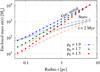 |
Fig. 7 Cumulative mass m(r) vs. the three-dimensional radius r for the gas initially (plain symbols) and the stars at t = 2 Myr (open symbols) with density indices p0 quoted in the key. For a power-law density profile of index p0 (Eq. (1)), the slope of the mass distribution in the r − m(r) space is 3 − p0 (Eq. (21)). The steeper density profiles of the stellar component thus lead to r − m(r) relations shallower than their initial gas analogs (i.e. 3 − q vs. 3 − p0). Note that the slope of the stellar tracks get steeper towards the clump centre due to the shallower stellar density profiles there. The dash-dotted symbol-free line has a slope of 0.5, as expected for the r − m(r) relation of the stellar component in the low-density regime when p0 = 1.7, i.e. 3 − q ≃ 3−3p0/2 = 0.5. While it indeed fits the model with p0 = 1.7 well in the clump ’s outer regions (green open symbols; r ≳ 1 pc), the deviation increases towards the clump centre as the stellar density profile gets shallower than q = 3p0/2 (see middle panel of Fig. 1). |
For an assumed volume density profile of the stellar component, one can extrapolate the
mass of the embedded cluster to that of the whole stellar component by representing the star
mass distribution in the r − m(r) space.
Figure 7 illustrates the relations between the
distance r from the star-forming region centre and the enclosed mass
m(r), for the gas initially and the stellar component at
t = 2 Myr. For a pure power-law density profile of index
p0, radii and masses follow (taking the case of the initial
gas density distribution, Eq. (1)):
 (21)We note that a steeper
volume density profile shows up as a shallower
r − m(r) relation (e.g. in Fig. 7, the gas tracks are steeper than their star analogues).
The tracks provide a direct mapping of how much stellar mass is enclosed within a given
radius. For instance, when p0 = 1.7 and
t = 2 Myr, the embedded cluster has a radius
recl ≃ 1 pc and a mass
mecl ≃ 400 M⊙, while the
stellar mass enclosed within R ≃ 6 pc is
≳103 M⊙.
(21)We note that a steeper
volume density profile shows up as a shallower
r − m(r) relation (e.g. in Fig. 7, the gas tracks are steeper than their star analogues).
The tracks provide a direct mapping of how much stellar mass is enclosed within a given
radius. For instance, when p0 = 1.7 and
t = 2 Myr, the embedded cluster has a radius
recl ≃ 1 pc and a mass
mecl ≃ 400 M⊙, while the
stellar mass enclosed within R ≃ 6 pc is
≳103 M⊙.
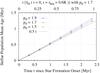 |
Fig. 8 Relation between the time t elapsed since the onset of star formation in the simulations and the mean age of the stellar component. Owing to the ongoing gas depletion and the star formation slow down that it induces, the mean age is slightly older than half the simulation time span. The bottom x-axis shows the physical time (i.e. time in units of Myr) while the top x-axis shows time in units of the initial local free-fall time at the clump half-mass radius, τff(t = 0,rhm) when p0 = 1.7. |
Finally, we note that the time t of our model corresponds to the age spread of the model stellar component. It differs from the mean age of the stars that would be inferred by an observer. Figure 8 illustrates the mass-weighted mean age of the stars against the time span t of the simulations. In the case of a constant star formation rate, the mean age is simply 0.5 t. However, in our model, star formation slows down with time and the first stars to form (i.e. the oldest ones) tend to dominate the mass budget. The mean age is therefore higher than 0.5 t, although the deviation is moderate, at most 10% of half the simulation time span. The effect is stronger for p0 = 1.9 than for p0 = 1.5 since a steeper gas density gradient slows down star formation more than a shallow one (see Sect. 4.1.1 and Fig. 9 below).
The top x-axis of Fig. 8 shows the time t since star formation onset in units of the initial local free-fall time at the clump half-mass radius, rhm, when p0 = 1.7. Using Eq. (21), we find rhm ≃ 0.6R for p0 = 1.7, which leads to an initial local density ρ0(rhm) ≃ 12 M⊙ pc-3 (Eq. (1)) and an initial local free-fall time τff(t = 0,rhm) ≃ 2.4 Myr. A scaling in units of the initial free-fall time enables us to apply our model to molecular clumps with different mean densities and, therefore, different rates of star formation (since the mass of newly formed stars depends on the ratio t/τff(t = 0,r); see e.g. Eq. (5)). For instance, a molecular clump that is 100 times denser initially forms stars at a rate that is 10 times faster (i.e. the bottom x-axis of Fig. 8 shrinks by a factor of 10). This density-dependent star formation rate is akin to the density-dependent rate of dynamical evolution of star clusters after gas expulsion studied in depth by Parmentier & Baumgardt (2012).
4. Model consequences
4.1. Star formation efficiencies: global and local
4.1.1. Global star formation efficiency
Figure 9 shows the evolution with time of the global star formation efficiency, SFE, namely, the stellar mass fraction averaged over the whole molecular clump: SFE = M ⋆ /M0. The density indices of the precursor clump are identical to those in Fig. 1, i.e. p0 = 1.5,1.7, and 1.9 (see key). The symbol-free lines depict the tangents to the models at the onset of star formation. A steeper density profile concentrates a higher gas mass fraction into the clump inner regions, which have higher densities and shorter free-fall times. This accelerates star formation initially (i.e. the tangent for p0 = 1.9 is steeper than for p0 = 1.5) and leads to higher global star formation efficiencies (see also Tan et al. 2006). With the ongoing gas depletion, star formation slows down as the comparison between the symbol-free lines and the numerical models illustrates. We note that, by a time t = 2.5 Myr, the global SFE remains low, at 0.1−0.15. We discuss this result in the framework of star cluster survival in Sect. 4.2. We also recall that the predicted SFEs are dependent on parameters (here M0 = 104 M⊙, R = 6 pc and ϵff = 0.1). Higher clump masses or smaller radii would lead to higher star formation efficiencies at any given time t.
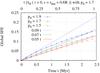 |
Fig. 9 Global star formation efficiency, SFE, in dependence of the time elapsed since the onset of star formation, t, for different initial density indices of the parent molecular clump, p0 (see key). The symbol-free lines illustrate the tangents to the numerical models at t = 0. Units of x-axes as in Fig. 8. |
4.1.2. Radially-varying local star formation efficiencies: two- and three-dimensional
To define the three-dimensional local star formation efficiency at distance
r from the clump centre, we build on the local volume densities of
stars and gas:  (22)We remind the
reader that the subscript “0” refers to the gas clump prior to star formation.
Equation (22) is illustrated in the
top panel of Fig. 10 for the same model as
previously at a time t = 2 Myr. As already introduced through the top
panel of Fig. 1, the local star formation
efficiency is higher in the clump centre than in its outskirts. It is worth keeping in
mind that the derived efficiencies depend on the adopted star formation efficiency per
free-fall time, on the assumed duration of the star-formation process, and on the clump
mean volume density. That is, a higher ϵff, longer
time t and/or a larger clump mean volume density
3M0/(4πR3)
would each increase ϵ3D(r). Also note that
steeper density profiles achieve higher values of ϵ3D since
the clump central density is then higher.
(22)We remind the
reader that the subscript “0” refers to the gas clump prior to star formation.
Equation (22) is illustrated in the
top panel of Fig. 10 for the same model as
previously at a time t = 2 Myr. As already introduced through the top
panel of Fig. 1, the local star formation
efficiency is higher in the clump centre than in its outskirts. It is worth keeping in
mind that the derived efficiencies depend on the adopted star formation efficiency per
free-fall time, on the assumed duration of the star-formation process, and on the clump
mean volume density. That is, a higher ϵff, longer
time t and/or a larger clump mean volume density
3M0/(4πR3)
would each increase ϵ3D(r). Also note that
steeper density profiles achieve higher values of ϵ3D since
the clump central density is then higher.
The three-dimensional local star formation efficiency
ϵ3D(r) is not the star formation
efficiency inferred by observers, however, since observers work with surface densities
rather than volume densities. We therefore define a two-dimensional star formation
efficiency based on the observed surface densities:  (23)Equation (23) is shown in the bottom panel of
Fig. 10.
(23)Equation (23) is shown in the bottom panel of
Fig. 10.
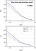 |
Fig. 10 Top panel: three-dimensional local star formation efficiency, ϵ3D, as a function of radius r (Eq. (22)) for different density indices p0 (see key in bottom panel). The progenitor clump of the star-forming region is the same as previously, i.e. M0 = 104 M⊙, R = 6 pc, and ϵff = 0.1. The time elapsed since the onset of star-formation is t = 2 Myr. Bottom panel: same for the two-dimensional star formation efficiency, ϵ2D, as a function of projected radius s (Eq. (23)). |
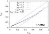 |
Fig. 11 Two-dimensional star formation efficiency, ϵ2D (Eq. (23)) against its three-dimensional counterpart, ϵ3D (Eq. (22)). The (black) dotted and solid lines correspond to ϵ2D = ϵ3D and ϵ2D = ϵ3D − 0.20. ϵ2D, the observed efficiency, is lower than ϵ3D, the actual efficiency, because surface densities measured around the clump centre intercept clump outskirts where the gas volume density and ϵ3D are lower. |
At a given radius s = r, ϵ2D(s) is lower than ϵ3D(r). This is so because the star surface densities in the clump centre vicinity intercept outskirt material where the initial gas volume densities and achieved star formation efficiencies are lower. This is illustrated further in Fig. 11, which depicts ϵ2D in dependence on ϵ3D. For the case of relevance here, the difference between the – measured – two-dimensional and – actual – three-dimensional star formation efficiencies can be as high as 20 per cent.
Both ϵ3D and ϵ2D rise from a few per cent at the clump edge up to higher than 50 per cent at the clump centre. In particular, star formation depletes almost the entirety of the initial gas content in the clump centre, and ϵ3D reaches values as high as 60−90% in the inner r ≲ 0.1 pc. This contrasts with the low global star formation efficiency, SFE, which we saw in Fig. 9. This has important consequences for the survivability of (part of) the stellar component as a bound cluster after residual gas expulsion, as we discuss in Sect. 4.2. The high central star formation efficiencies also allow us to propose an alternative explanation of the low gas content in the central regions of the most evolved molecular clumps of Higuchi et al. (2009). According to Higuchi et al. (2009), this absence or scarcity of gas results from its ongoing dispersal. In contrast, in our picture, the absence of gas in the central regions of developed embedded clusters (e.g. the Orion Nebula Cluster) or of Higuchi et al. (2009) clumps stems from most of it having been fed to star formation, even before gas dispersal starts.
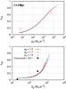 |
Fig. 12 Top panel: three-dimensional star formation efficiency, ϵ3D, in dependence of the initial gas volume density, ρ0. The clump edge is on the left, the clump centre on the right. The two vertical lines mark the limits of the p0 = 1.5 model. Bottom panel: two-dimensional star formation efficiency, ϵ2D, in dependence on the residual gas surface density, Σg. The plain squares depict the measurements of Gutermuth et al. (2011). In both panels, the models are identical to those in Figs. 10 and 11. |
The top panel of Fig. 12 shows how the three-dimensional star formation efficiency increases from a few per cent to almost unity as the initial gas volume density rises from a few M⊙ pc-3 (near the clump edge) to higher than 104 M⊙ pc-3 (toward the clump centre). We stress again that other model parameters will be conducive to different efficiencies. With ρ0 ≃ 7 M⊙ pc-3 ≡ nH2 ≃ 100 cm-3 and ρ0 > 7000 M⊙ pc-3 ≡ nH2 > 105 cm-3, where nH2 is the molecular hydrogen number density, the range of volume densities characterizing the molecular clump under scrutiny here extends from the diffuse molecular gas probed in C12O up to the dense gas traced in CS (e.g. Shirley et al. 2003) or dust continuum emission (e.g. Schuller et al. 2009).
The bottom panel of Fig. 12 illustrates the 2-dimensional star formation efficiency in dependence of the residual gas surface density, that is, ϵ2D versus Σg. This is the relation that would be inferred from observing the star-forming region. The measurements made by Gutermuth et al. (2011), ϵ2D = 2.3% and 26% at Σg = 20 and 300 M⊙ pc-2, are also shown. They are practically consistent with our model despite it not being based on detailed star and gas density profiles. It is interesting to note that star formation efficiencies of the order of 1% happen at gas surface densities that are only slightly higher than the limit beyond which the gas becomes entirely molecular in spiral galaxies, i.e. Σ = 9 M⊙ pc-2 (see top left panel in Fig. 8 of Bigiel et al. 2008). Therefore, the lowest star formation efficiencies would correspond to the lowest possible surface densities where the gas is entirely molecular (but see Lada et al. 2010).
Finally, Fig. 13 is the analogue of Fig. 9 for the local star formation efficiency, of which it shows the evolution with time for different radii r and density indices p0. At the low density of the clump outskirts (e.g. r = 5.6 pc), the small gas depletion is conducive to ϵ3D increasing linearly. In contrast, at r = 0.15 pc, the strong gas depletion slows down star formation and the local star formation efficiency evolution eventually tends to saturate.
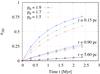 |
Fig. 13 Time evolution of the local star formation efficiency ϵ3D for three different distances r from the clump centre (see labels on the right) and three gas initial density indices p0 (see key) |
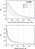 |
Fig. 14 Top panel: relations between the local three-dimensional star formation efficiency, ϵ3D(r), and the enclosed stellar mass fraction, m ⋆ (≤ r)/M ⋆ . Bottom panel: ϵ3D(r) against normalized radius, r/R, where R is the outer radius of the star-forming region. Symbol/colour-coding identical to Figs. 9−13 |
4.2. Radially-varying local star formation efficiency and cluster survival
Figure 9 shows that at the end of our simulations, the star formation efficiency averaged over the whole star-forming region remains low, SFE ≃ 10−15%. At first glance, this is significantly less than the threshold required for the stellar component to retain a bound star cluster after residual gas expulsion. The relation between SFE and the fraction of stars remaining bound to the stellar component, Fbound, is shown in Fig. 1 of Parmentier & Gilmore (2007) based on the simulations of Geyer & Burkert (2001) and Baumgardt & Kroupa (2007). For the sake of clarity, this Fbound-vs.-SFE relation is reproduced in our Fig. 15. It assumes instantaneous gas expulsion and a weak external tidal field. The threshold for retaining a bound group of stars (Fbound > 0) is SFEth ≃ 0.33. We stress that this threshold necessarily depends on the hypotheses of the models used to derive it. The vast majority of cluster-gas-expulsion models developed so far assume that the local star formation efficiency is uniform throughout the star-forming region; that is, ϵ3D is independent of r and constant (as a result SFE = ϵ3D). This is in stark contrast to our result in Sect. 4.1 that the local star formation efficiency spans nearly two orders of magnitude, from almost unity down to a few per cent (top panel of Fig. 10). This property of the star-forming region has important implications for the ability of the stellar component to retain a bound star cluster after gas expulsion. Owing to its small residual gas fraction, the clump central region has high resilience to gas expulsion. It will therefore necessarily produce a bound cluster. Most of the gas-expulsion-driven disruption of the stellar component takes place in the outskirts where the local star formation efficiency is low.
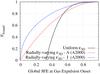 |
Fig. 15 Relation between the mass fraction of the stellar component forming a bound cluster after violent relaxation, Fbound, and the global SFE of the star-forming region. The solid (black) line, taken from Parmentier & Gilmore (2007), corresponds to a uniform local star formation efficiency (i.e. ϵ3D(r) = SFE irrespective of r). The dashed and dash-dotted lines (blue and red) depict the models with radially varying star formation efficiencies of Adams (2000) (i.e. ϵ3D(r) higher at smaller r than at large r). They build on either an isotropic (“I”, see key) or anisotropic (“A”) stellar velocity distribution. |
The top panel of Fig. 14 shows the local star formation efficiency in dependence on the enclosed stellar mass fraction. The bottom panel depicts ϵ3D against the normalized radius r/R (i.e. another representation of the top panel of Fig. 10, with the x-axis scale now linear). We now consider the model with a density index p0 = 1.9. About 15% of the stellar mass arises from gas having experienced a local star formation efficiency ϵ3D ≥ 0.60. Under the assumption of a uniform star formation efficiency in that limited central region (0.60 ≤ ϵ3D ≤ 0.95 when r/R ≤ 0.04 or r ≤ 0.25 pc; see bottom panel of Fig. 14), we can use the corresponding relation in Fig. 15 to infer the bound fraction of stars after violent relaxation. More than 85% of the stellar mass remains bound in the central region. We can now derive a lower limit on the mass of a surviving bound cluster. With a global SFE of ≃ 13% at a time t = 2 Myr (Fig. 9), the whole stellar component has a mass M ⋆ ≃ 1300 M⊙, of which 15% is located in the central area practically unaffected by gas expulsion. Therefore, a cluster of at least 200 M⊙ will remain after violent relaxation in spite of the low global SFE. In other words, over the overall scale of the whole star-forming region, the bound fraction Fbound must be at least 15%.
Adams (2000) developed a pioneering model accounting for a radially-dependent local star formation efficiency, which quantifies the effect introduced above. That is, because of the high local star formation efficiency in the central regions (i.e. high ϵ3D at small r), a cluster survives gas expulsion (Fbound > 0) despite a low global star formation efficiency (low SFE). As a result, in the low-SFE regime, the radially-varying models predict the survival of a bound cluster after violent relaxation (Fbound > 0), while the uniform model predicts the full disruption of the stellar component (Fbound = 0). The relations he derived between SFE and Fbound are shown in Fig. 15. They correspond to isotropic and anisotropic stellar velocity distributions, respectively. For SFE ≃ 0.1−0.15, uniform-ϵ3D models predict the stellar component full disruption. In contrast, the radially-varying models of Adams (2000) give bound fractions as high as 20% to 50%. With M0 = 104 M⊙, SFE = 0.13 and Fbound ≃ 0.3, our star-forming region would thus give rise to a bound star cluster with a mass: Mcl = FboundSFEM0 ≃ 400 M⊙. This is in fair agreement with the lower limit of 200 M⊙ we derived above.
5. Discussion and future work
In this section, we first discuss how our results and those from hydrodynamics simulations of star formation relate to each other. We then touch on two aspects of our work, which we will refine in the near future, namely, the value of the star formation efficiency per free-fall time (ϵff), and the impact of the density profile of molecular clumps.
5.1. Clump density profile and embedded-cluster morphology
Müller et al. (2002) detected in their sample of star-forming molecular clumps a correlation between the clump radial density profile and mass, with higher-mass clumps being on average steeper (top panels of their Fig. 18). The observed p-index range (0.7 ≲ p ≲ 2.5) can now be related to the comprehensive set of adaptative-mesh refinement simulations performed by Girichidis et al. (2011). These simulations show that the initial gas density gradient of spherical molecular clumps is of paramount importance to the morphology of the star clusters they form. In clumps initially uniform in density, supersonic turbulence has the time to compress the gas in locally disconnected areas before global collapse sets in. This results in locally disconnected filaments and spatially distinct subclusters of sink particles. In contrast, centrally concentrated clumps (e.g. a Bonnor-Ebert or power law p0 = 1.5 density profile) form filaments that are more strongly connected and centrally concentrated because of the shorter time-scale for global collapse in the clump central region. This eventually favours the formation of one main central cluster (see Fig. 4 in Girichidis et al. 2011). The morphology of these single-block clusters – substructured or smooth power-law density profile – depends on the initial turbulent velocity field (Girichidis et al. 2012b). Solenoidal turbulence in Bonner-Ebert or p0 = 1.5 density profiles can produce embedded clusters with a smooth radial density profile. For instance, the embedded-cluster Q-parameter6 can be of the order of 1.2 (Figs. 11 and 12 in Girichidis et al. 2012b). We note that 0.9 ≲ Q ≲ 1.5 corresponds to a power-law density index 2 ≲ q ≲ 2.9 for the embedded cluster (see Table 1 in Cartwright & Whitworth 2004), a q-range which agrees well with our model predictions (see our Eq. (8): q ≲ 3p0/2 = 2.25 if p0 = 1.5). We caution, however, that our model does not account for the clump global collapse and is therefore not fully comparable to those of Girichidis et al. (2011). Finally, we note that these adaptative-mesh refinement simulations predict that the first stars form in the clump central region (Girichidis et al. 2012a). Once secondary stars form around the central objects, they accrete the infalling gas, preventing it from reaching the clump central region (“fragmentation-induced starvation”). This forces new protostars to form at increasingly large distance from the clump centre, an aspect which agrees well with the Pfalzner (2011) scenario.
If the correlation between the clump density index and mass found by Müller et al. (2002) is genuine (a bias arising from more massive sources being located at greater distances where the resolution is poorer cannot be fully excluded yet), one would expect shallow low-mass clumps to produce ensembles of subclusters, while steeper high-mass clumps would give rise to “single-block” clusters. Which mode of star cluster formation – subclustered or “single-block” – dominates the process of star formation then depends on the slope of the clump mass function. Observed mass function slopes are shallower than −2 (e.g. ≃−1.7, Kramer et al. 1998). High-mass clumps therefore dominate the star-forming gas mass, and most newly formed stars may thus originate from “single-block” clusters. Low-mass clumps and subcluster ensembles would dominate the cluster population only in terms of number.
Similarly to the uniform density profile of Girichidis et al. (2011), the end product of the hydrodynamics simulations of Bonnell et al. (2008) is an ensemble of subclusters (see Maschberger et al. 2010, for their merging history). This is not surprising since the gas cylinder they scrutinize is characterized by a weak density gradient along its main axis. Despite a low global SFE (SFE ≃ 0.15), their subclusters are gas-poor on a length scale of 0.1−0.2 pc, an effect of the accretion of gas onto sink particles and the accretion-induced subcluster shrinkage (Kruijssen et al. 2012). This is reminiscent of the locally high SFE achieved by the central region of our molecular clump despite a globally low one (Figs. 9 and 10). Note, however, that the respective embedded-cluster morphologies are different (subclustered in Bonnell et al. 2008 vs. a smooth radial density profile in our model). Given their high local SFE and small number of stars, the relaxation time of subclusters is short enough for their early dynamical evolution to be dominated by collisional stellar dynamics rather than violent relaxation. As a result, Moeckel et al. (2012) find that subclusters expand due to the scattering of their stars, eventually erasing the subcluster structure (see also Smith et al. 2008). We recall that these results hold for the low-mass end of the cluster mass spectrum (i.e. cluster mass of the order of 100 M⊙), typical of the solar neighbourhood.
Finally, we emphasize that the outcomes of smooth-particle hydrodynamics and adaptative mesh refinement simulations of star-forming regions necessarily depend on their input physics. It remains ill-known how including magnetic fields or radiative feedback (hence gas heating), or treating the protostars as extended gas spheres rather than sink particles, would affect the emerging properties of model star-forming regions. Additionally, these simulations do not currently access the regime of ab initio formation of high-mass clusters. This is up to at least two orders of magnitude higher than the gas and stellar masses covered so far. How relevant to the formation of high-mass clusters the physical processes at work inside low-mass clouds are remains an open question.
5.2. The star formation efficiency per free-fall time
To match the observed local star formation law of Gutermuth et al. (2011) with our model (M0 ≃ 104 M⊙, R ≃ 6 pc) at t = 2 Myr requires a star formation efficiency per free-fall time of ϵff = 0.1. We insist that the so-derived value of ϵff is parameter-dependent. A longer time t or a higher clump density (i.e. shorter free-fall time) would both lead to higher YSO surface and volume densities. That would require a lower ϵff to maintain the good match between the model and the scaling law averaging the observations shown in the top panel of Fig. 3.
At this stage, it is therefore premature to draw any conclusion about our ϵff estimate being an order of magnitude higher than derived by Krumholz & Tan (2007). Krumholz & Tan (2007) consider the fraction of the Milky Way star formation rate taking place in different classes of objects, from giant molecular clouds (number densities nH2 ≃ 100 cm-3) to HCN-traced molecular clumps (nH2 ≃ 6 × 104 cm-3). Building on the total mass of these objects in the Galaxy and on their mean density, they derive a star formation efficiency per free-fall time of about one per cent, independent of volume density (SFRff ≃ 0.01 in their notation; see their Eq. (1) and Fig. 5). On the other hand, in a study of individual molecular clouds, Evans et al. (2009) infer 0.03 ≤ SFRff ≤ 0.06 (their Sect. 4.3). This is intermediate between the estimate of Krumholz & Tan (2007) and ours.
Ideally, to derive ϵff in the framework of our model, we need the total masses of gas and stars enclosed within a given radius (not simply orders of magnitude as used in this introductory paper), as well as the time elapsed since the onset of star formation. In a forthcoming paper, we will apply our model to smaller scale molecular clumps with known size, gas mass, and star mass. This will allow us to put the comparison between our ϵff estimate, those of Evans et al. (2009) and Krumholz & Tan (2007) on a firm footing. The comparison will be especially interesting because these three works define a sequence of distinct spatial scales, from Galaxy-integrated star formation (Krumholz & Tan 2007) to star formation in individual molecular clouds (Evans et al. 2009) and star formation in individual molecular clumps (our work).
5.3. The time-evolving gas density profile of molecular clumps
Summing up the observed surface density profiles of the stars and (unprocesssed) gas in star-forming regions will provide a direct estimate of p0, the initial density index. In that respect, our assumption of a single p0-value valid over 6 pc in radius is probably an oversimplification. Pirogov (2009) finds that the density index of massive-star-forming clumps is p = 1.6 ± 0.3 within 0.8 pc from their centre. Beyond that distance, the density profile drops more steeply. Beuther et al. (2002) reach a similar result for the massive star-forming regions they study. Two power laws are needed to describe their clump density profiles: p = 1.6 ± 0.5 within 32′′ from the clump centre, and a steeper density profile beyond (their Fig. 2). The break at 32′′ corresponds to half of their fittable range and equal 1 pc at the typical 6 kpc distance of their star-forming regions. Therefore, it will be interesting in the future to convert our present one-zone model into a two-zone one and to quantify how this affects the estimate of ϵff.
In addition, it is worth noting that the density indices reported by Beuther et al. (2002), Müller et al. (2002), and Pirogov (2009) refer to star-forming molecular clumps. Nevertheless, the bottom panel of Fig. 1 shows that, as the stellar content builds up, the gas density profile gets shallower, again reflecting the faster gas-to-star conversion in the clump inner regions. Over the radial range 0.2−1.0 pc and over a time-span of 2.5 Myr, this gas density profile evolves from p0 = 1.7 to p ≃ 1.3. It is therefore likely that observed star-forming molecular clumps had at star formation onset steeper profiles than is observed now. Models starting with p0 = 1.9 may thus be more appropriate than those with p0 = 1.5 or p0 = 1.7. One way of testing this observationally would be to compare the density profiles of starless molecular clumps (e.g. Tackenberg et al. 2012) and star-forming ones.
6. Summary and conclusions
We have presented a model quantifying the stellar content of molecular clumps as a function of time and initial gas volume density. The model key ingredient is the star formation efficiency per free-fall time, ϵff, namely, the mass fraction of gas turned into stars per free-fall time, τff (Eq. (2)). The model’s originality resides in it building on a local free-fall time defined in relation to the local volume density of the star-forming gas; that is, the radial volume density gradient of molecular clumps leads to a radially-dependent free-fall time, shorter in the clump central regions and longer in the clump outskirts. In other words, star formation proceeds more quickly at a shorter distance from the clump centre. As a result of this differential rate of star formation, the radial density profile of the stellar population built by the clump (which we referred to as the “stellar component”) is steeper than that of the clump initially (i.e. q ≲ 3p0/2, where q and p0 are, respectively, the density indices of the stellar component and of the clump initially; see Eq. (8)).
We combined the volume density profile of spherical molecular clumps (Eq. (1)) with their radially-dependent free-fall time (Eq. (2)) to model the density profile of the stellar component as a function of time and gas initial density. This was done both numerically (Sect. 2.2) and analytically (Sect. 2.3).
We then projected the volume density profiles for the unprocessed gas and stars and
obtained the corresponding surface density profiles (Sect. 2.4). Under the assumptions that YSOs do not migrate away from their birth sites
significantly, and that molecular clumps do not experience significant gas motions and/or
inflows and/or outflows, predicted surface density profiles were compared to the
observations. Specifically, we considered the local star formation law inferred by Gutermuth et al. (2011). It relates the local surface
density of molecular gas, Σg, and the local surface density of YSOs,
Σ ⋆ :  , with
α ≃ 2 and the surface densities in units of
M⊙ pc-2. We found that a stellar density
profile steeper than a gas density profile, as predicted by our model (Eq. (7) and top panel of Fig. 1), naturally leads to α > 1, as
observed by Gutermuth et al. (2011). In particular,
molecular clump density indices p0 in the range
1.5 ≤ p0 ≤ 1.9 are conducive to α ≃ 2, in
excellent agreement with what is observed.
, with
α ≃ 2 and the surface densities in units of
M⊙ pc-2. We found that a stellar density
profile steeper than a gas density profile, as predicted by our model (Eq. (7) and top panel of Fig. 1), naturally leads to α > 1, as
observed by Gutermuth et al. (2011). In particular,
molecular clump density indices p0 in the range
1.5 ≤ p0 ≤ 1.9 are conducive to α ≃ 2, in
excellent agreement with what is observed.
To compare the normalizations of the observed and predicted star formation laws, we considered the specific case of a molecular clump with an initial gas mass M0 ≃ 104 M⊙ and a radius R ≃ 6 pc. These mass and radius were chosen so as to emulate the most prominent concentration of YSOs in the MonR2 molecular cloud (Sect. 2.2). We found that the predicted star formation law agrees with its observed counterpart about 2 Myr after the onset of star formation (i.e. t = 2 Myr) for a star formation efficiency per free-fall time ϵff = 0.1. For that same model, we derived the YSO surface-density distribution (Sect. 2.5; Fig. 4) and found good agreement with the observed distribution of the solar neighbourhood inferred by Bressert et al. (2010). We stress that this comparison is only preliminary given that our present model covers one single molecular clump, while the distribution of Bressert et al. (2010) encompasses several star-forming regions.
In the second part of the paper, we combined our model of a time-evolving star-forming region with a surface density threshold (Sect. 3). Prior to the one-to-one identification of YSOs based on their infrared excess with the Spitzer telescope, the subtraction of a given surface density accounting for the contaminating foreground and background stars was often relied on to define the limiting radius of a cluster and its mass. The combination of our model predictions with a surface density threshold can thus be compared with pre-Spitzer cluster data sets, such as the star-cluster catalogue compiled by Lada & Lada (2003).
Pfalzner (2011) finds that the clusters of Lada & Lada (2003) define a sequence of
decreasing volume density along with increasing radius. She suggests that this sequence is a
time sequence corresponding to the growth of the cluster stellar content, a hypothesis we
confirm. As time goes by, the total stellar mass increase raises the fraction of the stellar
component seen above the surface density threshold. Therefore, the observed embedded-cluster
radius gets larger too (bottom panel of Fig. 5). The
mean surface density of the embedded cluster remains approximately constant since the
cluster definition rests on a surface density limit. A constant surface density equals to
,
the observed growth of the embedded-cluster radius thus leads to a decrease in the observed
mean volume density. In contrast, the outer radius of the stellar component as a whole stays
constant, and its mean volume density increases with time (see top panel of Fig. 6).
In Sect. 4, we discussed the impact of a radially-varying local star formation efficiency on the post-gas-expulsion evolution of clusters. That the density profile of the stellar component built by the clump is steeper than that of the gas initially implies a local star formation efficiency increasing towards the clump centre. As a result, the clump central region is more resilient to gas expulsion than the clump outskirts. Despite a low global star formation efficiency (SFE ≃ 10−15% at t = 2 Myr for M0 ≃ 104 M⊙, R ≃ 6 pc and ϵff = 0.1, see Fig. 9), the stellar component can still leave a bound cluster after violent relaxation due to the high local star formation efficiency (ϵ3D) in the clump innerst regions (Fig. 10).
Although our model addresses the formation of leaky (i.e. low-density) clusters, it already provides a hint as to why some starburst (i.e. high-density) clusters may be in virial equilibrium despite their very young age (e.g. Westerlund-1, Mengel & Tacconi-Garman 2007). We showed that volume densities characteristic of starburst clusters (i.e. several 103 M⊙ pc-3 at least) lead to three-dimensional star formation efficiencies in excess of 50% (Fig. 12; for the star formation efficiency per free-fall time adopted here). A high star formation efficiency limits the impact of gas expulsion on the cluster dynamics and the departure from virial equilibrium after gas expulsion. (In addition, a high density also implies a short crossing-time that hastens the return of the cluster to equilibrium, Parmentier & Baumgardt 2012.) That does not imply that gas expulsion is not a major driver of young cluster dynamics in general. Only high-density regions – e.g. dense molecular clumps close to the Galactic centre and central regions of massive molecular clumps in the Galactic disc, may be relatively immune to gas expulsion.
Finally, we note that a sound quantification of the stellar component also requires an accurate estimate of the star formation efficiency per free-fall time (ϵff) since this parameter drives the relation between the local star formation efficiency ϵ3D and the local volume density ρ0(r) at a given time. Should ϵff be halved, the predicted global and local star formation efficiencies will be reduced by a factor of two (at most). Here a direct connection arises between the rate of star formation in molecular clumps and the stellar dynamics of post-gas-expulsion clusters; that is, the rate of dissolution of young clusters and the star formation efficiency per free-fall time are closely related.
An alternative explanation to the C18O depletion, however, could be that C18O is frozen out on grain surfaces. Observations of the less-affected nitrogen-containing species NH3 and N2H+ should help clarify the question (Bergin et al. 2002).
Krumholz & McKee (2005) use the terminology “star formation rate per free-fall time”, or SFRff for short. We prefer to refer to the “star formation efficiency per free-fall time” and denote it as ϵff.
We refer to the Gutermuth et al. (2011) star formation law as a local law to make it distinct from the global star formation law of Kennicutt (1998), which builds on galaxy-integrated surface densities.
Strictly speaking, the density indices inferred by Beuther et al. (2002) and Müller et al. (2002) characterize star-forming molecular clumps. They may thus be different from p0, which in this model, is the gas density index prior to star formation. We come back to this point in Sect. 5.3.
Violent relaxation is the dynamical response of the stellar component to the expulsion of the unprocessed star-forming gas. Its duration – from ≃ 1 Myr to several tens of Myr – depends on the crossing-time of the cluster gaseous precursor and on the observed cluster region. The denser the gas clump (i.e. the shorter its mean crossing-time), the smaller the aperture with which the cluster is observed (i.e. the higher the observed cluster density), the faster the cluster evolution (Parmentier & Baumgardt 2012).
The Q-parameter (Cartwright & Whitworth 2004) quantifies the degree of substructures in star clusters. It is defined as the ratio between the normalized mean separation of the stars and the normalized mean length of the edges of the minimal spanning tree associated to the (proto)cluster. A cluster with Q < 0.8 is substructured/fractal, while Q > 0.8 indicates a smooth radial density profile.
Acknowledgments
Throughout this work, G.P. has been supported by a Research Fellowship of the Max-Planck-Institut für Radioastronomie (Bonn), and an Olympia-Morata Fellowship of Heidelberg University. We thank Karl Menten for a careful reading of our manuscript, and the referee, Cathie Clarke, for a very constructive report.
References
- Adams, F. 2000, ApJ, 542, 964 [NASA ADS] [CrossRef] [Google Scholar]
- Adams, F. 2006, ApJ, 641, 504 [NASA ADS] [CrossRef] [Google Scholar]
- Allen, L., Megeath, S. T., Gutermuth, R., et al. 2007, Protostars and Planets V, eds. B. Reipurth, D. Jewitt, & K. Keil (Tucson: University of Arizona Press), 951, 361 [Google Scholar]
- Bate, M. R., Bonnell, I. A., & Bromm, V. 2003, MNRAS, 339, 577 [NASA ADS] [CrossRef] [Google Scholar]
- Baumgardt, H., & Kroupa, P. 2007, MNRAS, 380, 1589 [NASA ADS] [CrossRef] [Google Scholar]
- Baumgardt, H., Parmentier, G., Gieles, M., & Vesperini, E. 2010, MNRAS, 401, 1832 [NASA ADS] [CrossRef] [Google Scholar]
- Bergin, E. A., Alves, J., Huard, T., & Lada, C. J. 2002, ApJ, 570, L101 [NASA ADS] [CrossRef] [Google Scholar]
- Beuther, H., Schilke, P., Menten, K. M., et al. 2002, ApJ, 566, 945 [NASA ADS] [CrossRef] [Google Scholar]
- Bigiel, F., Leroy, A., Walter, F., et al. 2008, AJ, 136, 2782 [NASA ADS] [CrossRef] [Google Scholar]
- Bonnell, I. A., Clark, P., & Bate, M. R. 2008, MNRAS, 389, 1156 [Google Scholar]
- Bressert, E., Bastian, N., Gutermuth, R., et al. 2010, MNRAS, 409, L54 [NASA ADS] [Google Scholar]
- Carpenter, J. M., Heyer, M. H., & Snell, R. L. 2000, ApJS, 130, 381 [NASA ADS] [CrossRef] [Google Scholar]
- Cartwright, A., & Whitworth, A. P. 2004, MNRAS, 348, 589 [NASA ADS] [CrossRef] [Google Scholar]
- Chandar, R., Fall, S. M., & Whitmore, B. C. 2010, ApJ, 711, 1263 [NASA ADS] [CrossRef] [Google Scholar]
- DaCosta, G. S., Grebel, E. K., Jerjen, H., Rejkuba, M., & Sharina, M. E. 2009, AJ, 137, 4361 [NASA ADS] [CrossRef] [MathSciNet] [Google Scholar]
- Elmegreen, B. G. 2000, ApJ, 530, 277 [NASA ADS] [CrossRef] [Google Scholar]
- Elmegreen, B. G. 2007, ApJ, 668, 1064 [NASA ADS] [CrossRef] [Google Scholar]
- Elmegreen, B. G. 2008, ApJ, 672, 1006 [NASA ADS] [CrossRef] [Google Scholar]
- Enoch, M. L., Glenn, J., Evans, N. J., II., et al. 2007, ApJ, 666, 982 [NASA ADS] [CrossRef] [Google Scholar]
- Evans, N. J. II, Dunham, M. M., Jørgensen, J. K., et al. 2009, ApJS, 181, 321 [NASA ADS] [CrossRef] [Google Scholar]
- Geyer, M. P., & Burkert, A. 2001, MNRAS, 323, 988 [NASA ADS] [CrossRef] [Google Scholar]
- Gieles, M., Moeckel, N., & Clarke, C. J. 2012, MNRAS, 426, 11 [Google Scholar]
- Girichidis, Ph., Federrath, C., Banerjee, R., & Klessen, R. S. 2011, MNRAS, 413, 2741 [NASA ADS] [CrossRef] [Google Scholar]
- Girichidis, Ph., Federrath, C., Banerjee, R., & Klessen R. S., 2012a, MNRAS, 420, 613 [NASA ADS] [CrossRef] [Google Scholar]
- Girichidis, Ph., Federrath, C., Allison, R., Banerjee, R., & Klessen, R. S. 2012b, MNRAS, 420, 3624 [NASA ADS] [Google Scholar]
- Gutermuth, R. A., Pipher, J. L., Megeath, S. T., et al. 2011, ApJ, 739, 84 [NASA ADS] [CrossRef] [Google Scholar]
- Higuchi, A. E., Kurono, Y., Saito, M., & Kawabe, R. 2009, ApJ, 705, 468 [NASA ADS] [CrossRef] [Google Scholar]
- Higuchi, A. E., Kurono, Y., Saito, M., & Kawabe, R. 2010, ApJ, 719, 1813 [NASA ADS] [CrossRef] [Google Scholar]
- Kennicutt, R. C. 1998, ApJ, 498, 541 [NASA ADS] [CrossRef] [Google Scholar]
- Klessen, R. S., Burkert, A., & Bate, M. R. 1998, ApJ, 501, 205 [Google Scholar]
- Kramer, C., Stutzki, J., Röhrig, R., & Corneliussen, U. 1998, A&A, 329, 249 [NASA ADS] [Google Scholar]
- Kruijssen, J. M. D., Maschberger, Th., Moeckel, N., et al. 2012, MNRAS, 419, 841 [NASA ADS] [CrossRef] [Google Scholar]
- Krumholz, M. R., & McKee, C. F. 2005, ApJ, 630, 250 [NASA ADS] [CrossRef] [Google Scholar]
- Krumholz, M. R., & Tan, J. C. 2007, ApJ, 654, 304 [NASA ADS] [CrossRef] [Google Scholar]
- Lada, C. J., & Lada, E. A. 2003, ARA&A, 41, 57 [NASA ADS] [CrossRef] [Google Scholar]
- Lada, C. J., Lombardi, M., & Alves, J. 2010, ApJ, 724, 687 [NASA ADS] [CrossRef] [Google Scholar]
- Longmore, S. N., Rathborne, J., Bastian, N., et al. 2012, ApJ, 746, 117 [NASA ADS] [CrossRef] [Google Scholar]
- Maíz-Apellániz, J. 2001, ApJ, 563, 151 [NASA ADS] [CrossRef] [Google Scholar]
- Maschberger, Th., Clarke, C. J., Bonnell, I. A., & Kroupa, P. 2010, MNRAS, 404, 1061 [NASA ADS] [CrossRef] [Google Scholar]
- Mengel, S., & Tacconi-Garman, L. E. 2007, A&A, 466, 151 [NASA ADS] [CrossRef] [EDP Sciences] [Google Scholar]
- Moeckel, N., Holland, Ch., Clarke, C. J., & Bonnel, I. 2012, MNRAS, 425, 450 [NASA ADS] [CrossRef] [Google Scholar]
- Müller, K. E., Shirley, Y. L., Evans, N. J. II, & Jacobson, H. R. 2002, ApJS, 143, 469 [NASA ADS] [CrossRef] [Google Scholar]
- Parmentier, G., & Baumgardt, H. 2012, MNRAS, in press [arXiv:1209.0766] [Google Scholar]
- Parmentier, G., & Gilmore, G. 2007, MNRAS, 377, 352 [NASA ADS] [CrossRef] [Google Scholar]
- Parmentier, G., Goodwin, S. P., Kroupa, P., & Baumgardt, H. 2008, ApJ, 678, 347 [NASA ADS] [CrossRef] [Google Scholar]
- Parmentier, G., Kauffmann, J., Pillai, T., & Menten, K. M. 2011, MNRAS, 416, 783 [NASA ADS] [Google Scholar]
- Pfalzner, S. 2009, A&A, 498, 37 [Google Scholar]
- Pfalzner, S. 2011, A&A, 536, 90 [Google Scholar]
- Pfalzner, S., Kaczmarek, T., & Olczak, C. 2012, A&A, 545, A122 [NASA ADS] [CrossRef] [EDP Sciences] [Google Scholar]
- Pirogov, L. E. 2009, Astron. Rep., 53, 1127 [NASA ADS] [CrossRef] [Google Scholar]
- Schmeja, S., Kumar, M. S. N., & Ferreira, B. 2008, MNRAS, 389, 1209 [NASA ADS] [CrossRef] [Google Scholar]
- Schuller, F., Menten, K. M., Contreras, Y., Wyrowski, F., et al. 2009, A&A, 504, 415 [NASA ADS] [CrossRef] [EDP Sciences] [Google Scholar]
- Shirley, Y. L., Evans, N. J. II,, Young, K. E., et al. 2003, ApJS, 149, 375 [NASA ADS] [CrossRef] [Google Scholar]
- Smith, R., Slater, R., Fellhauer, M., Goodwin, S., & Assmann, P. 2011, MNRAS, 416, 383 [NASA ADS] [Google Scholar]
- Tan, J. C., Krumholz, M. R., & McKee, C. F. 2006, ApJ, 641, L121 [NASA ADS] [CrossRef] [Google Scholar]
- Tackenberg, Beuther, H., Henning, T., et al. 2012, A&A, 540, 113 [Google Scholar]
All Figures
|
Fig. 1 Top panel: initial gas volume density profiles (filled symbols) and their associated steeper stellar density profiles (open symbols). The latter are obtained from the numerical or analytical model one million years after star formation onset, i.e. t = 1 Myr, for three distinct p0 density indices (see key). The spherical molecular clump has a mass M0 ≃ 104 M⊙, a radius R ≃ 6 pc, and the star formation efficiency per free-fall time is ϵff = 0.1. Middle panel: stellar density profiles from the numerical model (lines with open symbols) for the times t and density indices p0 quoted in the key. Each symbol-free line is the corresponding analytical upper limit (Eq. (8)). Bottom panel: time evolution of the gas volume density profile for p0 = 1.7. The star-formation-driven depletion of the gas in the central region of the molecular clump – where the free-fall time is the shortest – is clearly highlighted. The symbol-free dotted line over the range 0.2−1 pc has a slope of −1.3, i.e. shallower than the initial slope −1.7. |
| In the text | |
|
Fig. 2 Surface density profiles from the numerical model. Lines with circles from top to bottom: the molecular clump gas initially, the unprocessed gas and the stellar component at t = 1 Myr (see key). The molecular clump is the same as in Fig. 1, and the initial gas density index is p0 = 1.7. The solid symbol-free line depicts a slope of −0.7 which is the slope expected for the initial surface density profile of the gas when p0 = 1.7. We note that in the clump outskirts, the actual surface density profile becomes increasingly steeper than the power-law approximation. |
| In the text | |
|
Fig. 3 Local surface density of YSOs, Σ ⋆ , in dependence on the local surface density of the unprocessed/observed gas, Σg. Top panel: models for a molecular clump of mass M0 = 104 M⊙, radius R = 6 pc, density index p0 = 1.7, a star formation efficiency per free-fall time ϵff = 0.1 and the times t quoted in the key. The dotted (black) line depicts the average star-formation law inferred by Gutermuth et al. (2011). The orange and brown polygons illustrate the associated scatter observed for the MonR2 and Ophiuchus molecular clouds, where it is the smallest. Middle panel: models for a time t = 2 Myr and three distinct density indices of the molecular clump, p0 = 1.5, 1.7, and 1.9. The normalization of the model hardly depends on p0. Bottom panel: same as top panel but completed with the time evolution of the gas and YSO surface densities at four projected distances s from the clump centre (s-labelled dotted black lines). |
| In the text | |
|
Fig. 4 Top panel: distribution of stellar surface densities predicted by our model for a clump of mass M0 ≃ 104 M⊙, radius R ≃ 6 pc, and star formation efficiency per free-fall time ϵff = 0.1 (clump density index p0 and time t since star formation onset are given in the key). Bottom panel: two p0 = 1.7 models are shown at time t = 1 Myr and t = 2 Myr for the same molecular clump as above (lines with open symbols). The dotted and dash-dotted (black) lines depict two Gaussians fitting their low-density regime. The solid (red) line is the Gaussian given by Bressert et al. (2010) to describe the observed local surface density distribution of YSOs in the solar neighbourhood. Mean and standard deviation of all three Gaussians are given in brackets. |
| In the text | |
|
Fig. 5 Top panel: time evolution of the volume density profile of the stellar component for the model of Sect. 2.2: M0 = 104 M⊙, R = 6 pc, ϵff = 0.1 along with p0 = 1.7. Model time spans t are given in the key. Bottom panel: time evolution of the corresponding surface density profiles superimposed with the surface density limit, Σbck, imposed by the stellar background against which the star-forming region is projected (Carpenter et al. 2000). The shaded area shows how the surface density threshold conceals the “wings” of the stellar component, leading to observed radii (red diamonds) smaller than the actual one, i.e. sbck < R. |
| In the text | |
|
Fig. 6 Top panel: mean volume density in dependence of radius for (i) the whole stellar component (vertical sequence of red circles at R = 6 pc); and (ii) the associated embedded cluster (decreasing sequence of blue circles on the left). The open circle size scales with the logarithm of the stellar mass. The embedded cluster refers to the part of the star-forming region seen above the stellar background against which it is seen projected (Σbck = 40 M⊙ pc-2, solid red line). As a result of the applied surface density cut-off, the predicted embedded-cluster sequence has a constant mean surface density. Also, it does not differ much from the observed embedded-cluster sequence defined by Pfalzner (2011) (dashed green line; see text for details). The times and stellar masses are given along the plotted sequences. Middle panel: mass in stars against radius, for the whole star-forming region (red vertical track to the right) and for the developing embedded cluster (blue track to the left). Quoted to the left of the sequences are the times elapsed since the onset of star-formation (in Myr). Bottom panel: same as the middle panel but for the mass-vs-time space. |
| In the text | |
|
Fig. 7 Cumulative mass m(r) vs. the three-dimensional radius r for the gas initially (plain symbols) and the stars at t = 2 Myr (open symbols) with density indices p0 quoted in the key. For a power-law density profile of index p0 (Eq. (1)), the slope of the mass distribution in the r − m(r) space is 3 − p0 (Eq. (21)). The steeper density profiles of the stellar component thus lead to r − m(r) relations shallower than their initial gas analogs (i.e. 3 − q vs. 3 − p0). Note that the slope of the stellar tracks get steeper towards the clump centre due to the shallower stellar density profiles there. The dash-dotted symbol-free line has a slope of 0.5, as expected for the r − m(r) relation of the stellar component in the low-density regime when p0 = 1.7, i.e. 3 − q ≃ 3−3p0/2 = 0.5. While it indeed fits the model with p0 = 1.7 well in the clump ’s outer regions (green open symbols; r ≳ 1 pc), the deviation increases towards the clump centre as the stellar density profile gets shallower than q = 3p0/2 (see middle panel of Fig. 1). |
| In the text | |
|
Fig. 8 Relation between the time t elapsed since the onset of star formation in the simulations and the mean age of the stellar component. Owing to the ongoing gas depletion and the star formation slow down that it induces, the mean age is slightly older than half the simulation time span. The bottom x-axis shows the physical time (i.e. time in units of Myr) while the top x-axis shows time in units of the initial local free-fall time at the clump half-mass radius, τff(t = 0,rhm) when p0 = 1.7. |
| In the text | |
|
Fig. 9 Global star formation efficiency, SFE, in dependence of the time elapsed since the onset of star formation, t, for different initial density indices of the parent molecular clump, p0 (see key). The symbol-free lines illustrate the tangents to the numerical models at t = 0. Units of x-axes as in Fig. 8. |
| In the text | |
|
Fig. 10 Top panel: three-dimensional local star formation efficiency, ϵ3D, as a function of radius r (Eq. (22)) for different density indices p0 (see key in bottom panel). The progenitor clump of the star-forming region is the same as previously, i.e. M0 = 104 M⊙, R = 6 pc, and ϵff = 0.1. The time elapsed since the onset of star-formation is t = 2 Myr. Bottom panel: same for the two-dimensional star formation efficiency, ϵ2D, as a function of projected radius s (Eq. (23)). |
| In the text | |
|
Fig. 11 Two-dimensional star formation efficiency, ϵ2D (Eq. (23)) against its three-dimensional counterpart, ϵ3D (Eq. (22)). The (black) dotted and solid lines correspond to ϵ2D = ϵ3D and ϵ2D = ϵ3D − 0.20. ϵ2D, the observed efficiency, is lower than ϵ3D, the actual efficiency, because surface densities measured around the clump centre intercept clump outskirts where the gas volume density and ϵ3D are lower. |
| In the text | |
|
Fig. 12 Top panel: three-dimensional star formation efficiency, ϵ3D, in dependence of the initial gas volume density, ρ0. The clump edge is on the left, the clump centre on the right. The two vertical lines mark the limits of the p0 = 1.5 model. Bottom panel: two-dimensional star formation efficiency, ϵ2D, in dependence on the residual gas surface density, Σg. The plain squares depict the measurements of Gutermuth et al. (2011). In both panels, the models are identical to those in Figs. 10 and 11. |
| In the text | |
|
Fig. 13 Time evolution of the local star formation efficiency ϵ3D for three different distances r from the clump centre (see labels on the right) and three gas initial density indices p0 (see key) |
| In the text | |
|
Fig. 14 Top panel: relations between the local three-dimensional star formation efficiency, ϵ3D(r), and the enclosed stellar mass fraction, m ⋆ (≤ r)/M ⋆ . Bottom panel: ϵ3D(r) against normalized radius, r/R, where R is the outer radius of the star-forming region. Symbol/colour-coding identical to Figs. 9−13 |
| In the text | |
|
Fig. 15 Relation between the mass fraction of the stellar component forming a bound cluster after violent relaxation, Fbound, and the global SFE of the star-forming region. The solid (black) line, taken from Parmentier & Gilmore (2007), corresponds to a uniform local star formation efficiency (i.e. ϵ3D(r) = SFE irrespective of r). The dashed and dash-dotted lines (blue and red) depict the models with radially varying star formation efficiencies of Adams (2000) (i.e. ϵ3D(r) higher at smaller r than at large r). They build on either an isotropic (“I”, see key) or anisotropic (“A”) stellar velocity distribution. |
| In the text | |
Current usage metrics show cumulative count of Article Views (full-text article views including HTML views, PDF and ePub downloads, according to the available data) and Abstracts Views on Vision4Press platform.
Data correspond to usage on the plateform after 2015. The current usage metrics is available 48-96 hours after online publication and is updated daily on week days.
Initial download of the metrics may take a while.