| Issue |
A&A
Volume 541, May 2012
|
|
|---|---|---|
| Article Number | A12 | |
| Number of page(s) | 89 | |
| Section | Interstellar and circumstellar matter | |
| DOI | https://doi.org/10.1051/0004-6361/201118640 | |
| Published online | 19 April 2012 | |
Galactic cold cores
III. General cloud properties⋆,⋆⋆,⋆⋆⋆
1
Department of Physics, PO Box 64, 00014, University of
Helsinki, Finland
e-mail: This email address is being protected from spambots. You need JavaScript enabled to view it.
2
Université de Toulouse, UPS-OMP, IRAP, 31028
Toulouse Cedex 4,
France
3
CNRS, IRAP, 9
Av. colonel Roche, BP
44346, 31028
Toulouse Cedex 4,
France
4
LERMA, CNRS UMR8112, Observatoire de Paris,
61 avenue de l’Observatoire,
75014
Paris,
France
5
LERMA, CNRS UMR8112, Observatoire de Paris and École Normale
Supérieure, 24 rue
Lhomond, 75005
Paris,
France
6
The University of Tokyo, Komaba 3-8-1, Meguro, Tokyo, 153-8902, Japan
7
IPAC, Caltech, Pasadena, USA
8
Laboratoire AIM Paris-Saclay, CEA/DSM – INSU/CNRS – Université
Paris Diderot, IRFU/SAp CEA-Saclay, 91191
Gif-sur-Yvette,
France
9
Konkoly Observatory of the Hungarian Academy of
Sciences, 1525
Budapest, PO Box
67, Hungary
10
Loránd Eötvös University, Department of Astronomy,
Pázmány P.s. 1/a, 1117 Budapest,
Hungary ( OTKA
K62304 )
11
IAS, Université Paris-Sud, 91405
Orsay Cedex,
France
12
Laboratoire d’Astrophysique de Marseille,
38 rue F.
Joliot-Curie, 13388
Marseille Cedex 13,
France
13
Finnish Centre for Astronomy with ESO (FINCA), University of
Turku, Väisäläntie
20, 21500
Piikkiö,
Finland
Received:
14
December
2011
Accepted:
7
February
2012
Abstract
Context. In the project galactic cold cores we are carrying out Herschel photometric observations of cold regions of the interstellar clouds as previously identified with the Planck satellite. The aim of the project is to derive the physical properties of the population of cold clumps and to study its connection to ongoing and future star formation.
Aims. We examine the cloud structure around the Planck detections in 71 fields observed with the Herschel SPIRE instrument by the summer of 2011. We wish to determine the general physical characteristics of the fields and to examine the morphology of the clouds where the cold high column density clumps are found.
Methods. Using the Herschel SPIRE data, we derive colour temperature and column density maps of the fields. Together with ancillary data, we examine the infrared spectral energy distributions of the main clumps. The clouds are categorised according to their large scale morphology. With the help of recently released WISE satellite data, we look for signs of enhanced mid-infrared scattering (“coreshine”), an indication of growth of the dust grains, and have a first look at the star formation activity associated with the cold clumps.
Results. The mapped clouds have distances ranging from ~100 pc to several kiloparsecs and cover a range of sizes and masses from cores of less than 10 M⊙ to clouds with masses in excess of 10 000 M⊙. Most fields contain some filamentary structures and in about half of the cases a filament or a few filaments dominate the morphology. In one case out of ten, the clouds show a cometary shape or have sharp boundaries indicative of compression by an external force. The width of the filaments is typically ~0.2–0.3 pc. However, there is significant variation from 0.1 pc to 1 pc and the estimates are sensitive to the methods used and the very definition of a filament. Enhanced mid-infrared scattering, coreshine, was detected in four clouds with six additional tentative detections. The cloud LDN 183 is included in our sample and remains the best example of this phenomenon. About half of the fields are associated with active star formation as indicated by the presence of mid-infrared point sources. The mid-infrared sources often coincide with structures whose sub-millimetre spectra are still dominated by the cold dust.
Key words: ISM: clouds / infrared: ISM / submillimeter: ISM / dust, extinction / stars: formation / stars: protostars
Planck (http://www.esa.int/Planck) is a project of the European Space Agency – ESA – with instruments provided by two scientific consortia funded by ESA member states (in particular the lead countries: France and Italy) with contributions from NASA (USA), and telescope reflectors provided in a collaboration between ESA and a scientific consortium led and funded by Denmark.
Herschel is an ESA space observatory with science instruments provided by European-led Principal Investigator consortia and with important participation from NASA.
Appendices A–E are available in electronic form at http://www.aanda.org
© ESO, 2012
1. Introduction
The main phases of the star formation process are largely understood, starting from molecular clouds and progressing via dense cores down to protostellar collapse (McKee & Ostriker 2007). This is thanks to the detailed observations of the nearest low mass and intermediate mass star formation regions and, on the other hand, sophisticated numerical modelling. However, the formation of each star is an individual process and, for a global view, extensive surveys of different environments and of the different phases of the star formation process are needed.
One major question is how the properties of star formation depend on the initial conditions within the cold molecular clouds. Direct links should exist between the physics of the prestellar clumps and the star formation efficiency, the mode of star formation (clustered vs. isolated), and the masses of the born stars (Elmegreen 2011; Padoan & Nordlund 2011; Nguyen Luong et al. 2011). The general time scales of star formation have been extensively studied. Eventually, one has to progress to the examination of the finer details, how the processes vary between different environments and, in each case, what is the interplay between turbulence, magnetic fields, kinematics, and gravity. Similarly, our understanding of the role of external triggering is incomplete. How does the influence of supernovae and stellar winds (and of galactic density waves, colliding flows of HI gas, etc.) vary between different regions of the Milky Way and is this reflected in the timescales and the stellar initial mass function?
The Planck satellite (Tauber et al. 2010) has made a new approach to the study of the earliest stages of star formation possible. By mapping the whole sky at several sub-millimetre wavelengths, with high sensitivity and small beam size (below 5′ at the highest frequencies), Planck is providing data for a global census of the coldest component of the interstellar medium. The selection of the cold (Tdust < 14 K) and “compact” (close to beam size) objects has led to a list of more than 10 000 objects. Because of the limited resolution, this Cold Clump Catalogue of Planck Objects (C3PO, see Planck Collaboration 2011c) is not dominated by cores (pre-stellar or only starless cores at sub-parsec scales) but by ~1 pc sized clumps and even larger cloud structures extending to even tens of pc in size. However, the low temperatures of the objects (below 14 K) are possible only for the denser, less evolved regions that are well shielded from the interstellar radiation field. Therefore, the objects detected by Planck are likely to contain one or several cores, many of which will be pre-stellar or in the early stages of protostellar evolution. This Planck survey constitutes the first unbiased census (in terms of sky coverage) of possible future star forming sites and provides a good starting point for global studies addressing the pre-stellar phase of cloud evolution.
Within the Herschel open time key programme Galactic cold cores, we are mapping selected Planck C3PO objects with the Herschel PACS and SPIRE instruments (100–500 μm). The higher spatial resolution of Herschel (Poglitsch et al. 2010; Griffin et al. 2010) makes it possible to examine the structure of the sources which gave rise to the Planck detections, often resolving the individual cores. The inclusion of shorter wavelengths (down to 100 μm) help to determine the physical characteristics of the sources and their environment, and to investigate the properties of the interstellar dust grains. Our Herschel survey will eventually cover some 120 fields between 12′ and one degree in size and will altogether cover approximately 350 individual Planck detections of cold clumps. Preliminary results of this follow-up have been presented in Juvela et al. (2010, 2011, Papers I and II, respectively) from the Herschel science demonstration phase observations (three fields there called PCC288, PCC249, and PCC550) and on a sample of ten Planck sources in Planck Collaboration (2011b).
In this paper we present results for the first 71 fields that were observed with the SPIRE instrument1 (250, 350, and 500 μm) by the summer 2011. We concentrate on the large scale structure of the clouds and the general characteristics of the main clumps. We compare the sub-millimetre emission with other available far-infrared data, especially the AKARI (Murakami et al. 2007) satellite far-infrared maps, and use Wide-field Infrared Survey (WISE Wright et al. 2010) satellite observations (3.6–22 μm) to look for regions where enhanced mid-infrared scattering could indicate an increase in the size of the dust grains. This so-called coreshine phenomenon was first detected with Spitzer data of LDN183 (see Steinacker et al. 2010), a cloud also included in the present sample. The point sources detected in the mid-infrared WISE data also serve as an indicator of the ongoing star formation.
The structure of the paper is the following. The observations are described in Sect. 2. The main results are presented in Sect. 3, starting with the analysis of the large scale properties of the clouds. These include the estimation of the colour temperatures (Sect. 3.1.1), the column densities, and cloud masses (Sect. 3.1.2), all based on the SPIRE observations. In Sect. 3.1.3 we describe a categorisation of the target fields that is based on the main cloud morphology. In Sect. 3.2 we characterise the fields further with the help of infrared data. We examine the properties of the selected clumps, present their spectral energy distributions and masses (Sect. 3.2.1) and then look for coreshine in the mid-infrared data (Sect. 3.2.2). The results concerning the general nature of the fields and the connection to the star formation are discussed in Sect. 4. The final conclusions are presented in Sect. 5. The appendices contain additional figures, including the surface brightness and the column density maps and the SEDs of selected clumps.
A detailed analysis of all compact sub-millimetre clumps (including the core mass spectra) and of the young stellar objects associated with the cold clumps will be presented in future papers. An in-depth study of dust emission properties (opacity and emissivity spectral indices) will also be presented later, together with the data from observations with the Herschel PACS instrument.
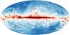 |
Fig. 1 The locations of the observed fields. The background is the IRAS 100 μm map and the circles denote the positions of the fields. The arrows drawn on each circle indicate the distances, starting with 0 pc for the upright direction, one clockwise rotation corresponding to 2 kpc. The six sources with distances larger than 1.5 kpc are drawn with smaller symbols. The sources without reliable distance estimates are marked with crosses. |
2. Observations
2.1. Target selection
The Planck satellite is performing surveys of the full sky at nine wavelengths between 350 μm and 1 cm (Tauber et al. 2010). The analysis of the first two sky surveys led to the detection of more than 10 000 compact sources of cold dust emission as described in Planck Collaboration (2011c). The detections are based on the sub-millimetre cold dust signature that becomes visible when the warm extended emission is subtracted using the IRAS 100 μm maps as its spatial template and the average spectrum of the region as its spectral template (Montier et al. 2010). The detection procedure limits the maximum size of the detected clumps to ~12′. Together with the IRAS 100 μm data, the Planck measurements have been used to estimate the colour temperatures of the sources. The source distances are estimated using several methods (see Planck Collaboration 2011c, for details) that include association with known molecular clouds complexes or individual sources and the reddening of background stars at optical or near-infrared wavelengths (Marshall et al. 2009; Mc Gehee, in prep.). Altogether distance estimates exist for approximately one third of the C3PO catalogue.
The pre-selection of targets for the Herschel observations was based on a binning of Planck cold clumps with the following parameter boundaries: l = 0, 60, 120, and 180 degrees, |b| = 1, 5, 10, and 90 degrees, Tdust = 6,9, 11, and 14 K, and M = 0, 0.01, 2.0, 500, 106 M⊙. Here Tdust is the clump temperature obtained after the subtraction of the warm emission component (see Planck Collaboration 2011c). The binning was used to ensure a full coverage of the respective parameter ranges while at the same time weighting the sampling towards sources at high latitudes and with extreme values of the mass. The lowest mass bin (M = 0) was reserved for sources without distance estimates and, therefore, without any available mass estimates. The Galactic latitudes |b| < 1° were excluded because those regions will be covered by the Herschel key programme Hi-GAL (Molinari et al. 2010). Similarly, the regions covered by the other key programmes like the Gould Belt survey (André et al. 2010) or HOBYS (Motte et al. 2010) were avoided.
The above procedure results in 108 bins, from which one target per bin was selected for Herschel follow up observations. Within each bin, the sources were inspected visually, comparing the Planck maps with IRAS and AKARI dust emission maps, extinction maps calculated using 2MASS stars, and CO emission maps (Dame et al. 2001; Fukui et al. 1999), when available. These data were used to confirm the reliability of the original detection. Some preference was given to fields containing several Planck detected clumps. The final selection of 108 fields covers some 350 cold clumps from the C3PO catalogue. Out of the full list of 108 fields, in this paper we use the SPIRE observations of the 71 fields for which the observations were completed by the Herschel observational day 721. In this sample, distance estimates exist for 75% of the fields (53 out of 71), partly because a literature search has resulted in a few additional distance estimates. Figure 1 shows the positions of the sources on the sky and Fig. 2 the distribution of their distances. For the fields with distance estimates, the median value is 450 pc. When distances were estimated from the stellar reddening (Marshall et al. 2009; Mc Gehee, in prep.), every effort was made to identify the extinction features most likely to be associated with the main clouds. However, the fields may contain clouds also at other distances, especially at the low Galactic latitudes. The distance distribution of all Planck clumps is smooth over the shown range of distances (Planck Collaboration 2011c). The small number statistics and the uncertainties of the distance estimates (e.g., the use of different methods in different distance ranges) may contribute to the dips seen in Fig. 2 at ~600 pc and ~1400 pc. The distribution is also affected by the exclusion of the areas covered by the other Herschel key programmes. In particular, the avoidance of the Gould Belt clouds reduces the number of objects close to 500 pc.
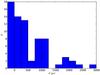 |
Fig. 2 The distance distribution of the fields. The bin at negative values corresponds to the sources without a distance estimate. |
2.2. Herschel observations
In this paper we use data from the first 71 fields observed with the Herschel SPIRE instrument. The observations consist of 250, 350, and 500 μm maps with the map sizes ranging from 37 to 77 arcmin. The observations of the first three sources were done as part of the Science Demonstration Phase in November and December 2009 and the latest were performed at the beginning of May 2011. The fields are listed in Table 1. The Herschel observations were reduced with the Herschel Interactive Processing Environment HIPE v.7.0. using the official pipeline2. The resulting SPIRE maps are the product of direct projection onto the sky and averaging of the time ordered data (the HIPE naive map making routine)3. In order of wavelength, the resolution of the SPIRE maps is 18″, 25″, and 37″, respectively.
The observed fields.
We rely on the Herschel calibration of the data. The accuracy of the absolute calibration of the SPIRE observations is expected to be better than 7%4. However, in order to determine the absolute zero point of the intensity scale, we carried out a comparison with Planck satellite observations that were complemented with the IRIS version of the IRAS 100 μm data (Miville-Deschênes & Lagache 2005). The Planck and IRIS measurements were interpolated to the Herschel wavelengths using fitted modified blackbody curves, Bν(Tdust)νβ, with a fixed value of the spectral index, β = 2.0. The linear correlations between Herschel and the reference data were extrapolated to zero Planck (+IRIS) surface brightness to determine the offsets for the Herschel maps. The uncertainties of the offsets were obtained from the formal errors of these fits. The errors are typically ~1 MJy sr-1 at 250 μm and, corresponding to the decreasing surface brightness values at the longer wavelengths. The derived intensity zero point is independent of the Planck calibration and any multiplicative errors included in the comparison. Similarly, the offset determination depends very little on the assumed value of β. Colour corrections can have an effect on the quality of the linear correlation between Planck and Herschel data. The data were first colour corrected assuming a constant colour temperature of 15 K. The offsets were later re-evaluated using the actual dust colour temperature estimates (Sect. 3.1.1).
2.3. Other infrared data
In the infrared range, we use data from the AKARI and WISE satellites.
From the AKARI survey (Murakami et al. 2007) we use observations from the all-sky survey made with the FIS instrument. These include observations in the narrow band filters N60 and N160 (central wavelengths 65 μm and 160 μm) and in the wide band filters WideS and WideL (central wavelengths 90 μm and 140 μm). The spatial resolution of the data ranges from 37″ at 65 μm to 61″ at 160 μm. The accuracy of the calibration is assumed to be ~30%. AKARI data are available for all the fields.
The WISE satellite (Wright et al. 2010) has four bands centred at 3.4, 4.6, 12.0, and 22.0 μm with spatial resolution ranging from 6.1″ at the shortest wavelength to 12″ at 22 μm. The first public release of WISE satellite data took place in April 2011 and it provides data for 55 of our 71 fields. We use the WISE 3.4 μm, and 4.6 μm data to look for signs of enhanced mid-infrared scattering and the WISE 12.0 μm and 22.0 μm data to characterise the mid-infrared dust emission and to look for indications of ongoing star formation. The data were converted to surface brightness units with the conversion factors given in the explanatory supplement (Cutri et al. 2011). The calibration uncertainty is ~6% for the 22 μm band and less for the shorter wavelengths.
We calculated dust extinction maps for each field with stars from the Two Micron All Sky Survey (2MASS, Skrutskie et al. 2006), using the NICER method (Lombardi & Alves 2001). The values of AV were obtained from near-infrared (NIR) colour excess measurements assuming an extinction law with RV = 3.1. With the assumption of RV = 5.5, possibly more appropriate for the densest regions, the AV estimates would increase by ~16% (see Juvela et al. 2011). The spatial resolution of all the produced extinction maps is two arcminutes. For distant sources, the extinction of the target clouds cannot be reliably reproduced because of the poor resolution and the increasing number of foreground stars. The same applies to some extent to the nearby, high latitude targets. No special steps have been taken to eliminate the contamination by foreground stars (see, e.g., Schneider et al. 2011), apart from the sigma clipping procedure (clipping performed at the 3-σ level) included in the NICER method. Therefore, the extinction maps should not be trusted unreservedly as tracers of the column density of the examined clouds. On the contrary, the possible discrepancy between the AV map and the sub-millimetre emission serves as an indicator of a large source distance.
3. Results
3.1. Cloud properties derived from SPIRE
In this section we present the results derived from the SPIRE data. These include colour temperature and column density maps and, when distance estimates are available, estimates of the cloud masses. In Sect. 3.1.4, we examine the properties of the filamentary cloud structures.
3.1.1. Colour temperature maps
The colour temperature maps of the large grain emission are estimated using the 250 μm, 350 μm, and 500 μm SPIRE maps with the main goal of identifying the coldest clumps. The data cover only the longer wavelength side of the dust emission peak which means that the derived temperatures may not be very accurate, especially for warm regions with temperatures close to 20 K or above. On the other hand, the absence of shorter wavelengths decreases the bias that results from temperature variations along the line of sight (Shetty et al. 2009b,a; Malinen et al. 2011). The statistical noise will be larger than, for example, if one included the PACS bands, but the values will be more representative of the bulk of the cold dust. The absence of data below or near 100μm also avoids the problem of a possible contribution from stochastically heated small grains.
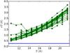 |
Fig. 3 Uncertainty of the colour temperatures estimated with a Monte Carlo study. The curves show, for each field, the mean error of the temperature if the uncertainty of the surface brightness data were 13%. The horizontal line is the 1-σ value (calculated over all fields) of the bias associated with the uncertainty of the intensity scale zero points. |
The maps were convolved to a 40 arcsec resolution and, for each pixel, the SED was fitted with Bν(Tdust)νβ keeping the spectral index β at a fixed value of 2.0. Several studies have suggested that the spectral index may increase in cold and dense environments (e.g. Dupac et al. 2003; Désert et al. 2008; Planck Collaboration 2011c). If this anticorrelation between the dust temperature and the spectral index is true also in our fields, the derived temperature maps will underestimate the range of temperature variations and, in particular, will overestimate the temperature of the coldest regions, leading to an underestimation of the masses of these regions (Planck Collaboration 2011c). However, the temperature maps will still fulfill their main purpose, identifying the major relative temperature variations within the regions.
The effect of statistical errors was examined with the help of Monte-Carlo simulations where a 13% uncertainty in the surface brightness values was assumed. Based on the correlations between the different bands, this is a conservative estimate and probably even twice the value of the typical true noise. The 13% uncertainty of the surface brightness values would translate to an error below 1 K in cold regions, the error increasing to ~3 K at 20 K (Fig. 3). The calibration accuracy of the SPIRE data is estimated to be 7%. This is well within the above limits.
The effect of the intensity zero points was estimated in a similar fashion, examining realisations of the temperature maps when the zero points were modified in accordance with the uncertainty of the comparison of Herschel and Planck/IRIS data. This uncertainty was less significant, typically less than 0.5 K and ~1 K in a few cases (G130.42-47.07, G161.55-9.30, G37.49+3.03). However, the effects on the relative temperature variations within a given field are, of course, much smaller. The temperatures can be further affected by mapping artifacts, e.g., residual striping. The striping is usually visible only towards the map edges where its effect can rise to ~0.5 K.
Two examples of calculated temperature maps are seen in frame a of Figs. 4 and 5. The colour temperature maps of all the fields are presented in Appendix A.
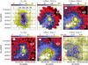 |
Fig. 4 Selected observed and derived quantities for the field G4.18+35.79 (LDN 134). Shown are the colour temperature map derived from SPIRE data (frame a, 40″ resolution), the 250 μm SPIRE surface brightness map (frame b, 18″ resolution), the AKARI wide filter maps at 140 μm and 90 μm (frames c and e), the visual extinction AV derived from 2MASS catalog stars (frame d), and the WISE 22 μm intensity (frame f). For the other fields, see Appendix A. The respective beam sizes are indicated in the lower right hand corner of each frame. The positions of selected clumps (black circles; see Sect. 3.2.1) and the reference regions used for background subtraction (white circle; see Sect. 3.2.1) are also shown. In frame b, the arrow indicates the position of the stripe plotted in Fig. 9. |
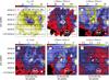 |
Fig. 5 Selected observed and derived quantities for the field G130.37+11.26 (see Fig. 4 for details). |
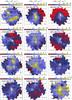 |
Fig. 6 Column density maps of the 12 first fields in the order of increasing Galactic longitude. The map resolution is 40″ and the areas are the same as in Fig. 4 and Appendix A. The colour scale has a square root scale. The column densities of the other fields are shown in Appendix B. |
3.1.2. Column density maps and masses
The column densities averaged over a 40″ beam are calculated using the formula
 (1)with the intensity and
temperature of the previous SED fits (Sect. 3.1.1)
and using μ = 2.33 for the particle mass per hydrogen molecule. We use
a dust opacity κ obtained from the formula
0.1 cm2/g (ν/1000 GHz)β that
is applicable to high density environments (Beckwith
et al. 1990). The value of dust opacity is uncertain and is observed to vary
from region to region (e.g. Kramer et al. 2003;
Stepnik et al. 2003; Lehtinen et al. 2004, 2007;
Ridderstad et al. 2006; Martin et al. 2012). In diffuse medium the expected value of
κ is lower by a factor of two (Boulanger et al. 1996). However, the value chosen here is close to the
predictions and the observations of dense clouds (e.g. Ossenkopf & Henning 1994; Nutter
et al. 2006, 2008) and also is the value
used in Planck Collaboration (2011c,b). The column density maps of the first eleven
sources are shown in Fig. 6 and for the rest in
Appendix B. The resolution of the maps is 40″.
(1)with the intensity and
temperature of the previous SED fits (Sect. 3.1.1)
and using μ = 2.33 for the particle mass per hydrogen molecule. We use
a dust opacity κ obtained from the formula
0.1 cm2/g (ν/1000 GHz)β that
is applicable to high density environments (Beckwith
et al. 1990). The value of dust opacity is uncertain and is observed to vary
from region to region (e.g. Kramer et al. 2003;
Stepnik et al. 2003; Lehtinen et al. 2004, 2007;
Ridderstad et al. 2006; Martin et al. 2012). In diffuse medium the expected value of
κ is lower by a factor of two (Boulanger et al. 1996). However, the value chosen here is close to the
predictions and the observations of dense clouds (e.g. Ossenkopf & Henning 1994; Nutter
et al. 2006, 2008) and also is the value
used in Planck Collaboration (2011c,b). The column density maps of the first eleven
sources are shown in Fig. 6 and for the rest in
Appendix B. The resolution of the maps is 40″.
Mass estimates are possible for the sources with distance estimates, i.e., 59 out of the 71 fields (see Table 1). Masses are calculated for the entire field, for some major filaments (see Sect. 3.1.4), and for one or two representative clumps within each field (see Sect. 3.2.1). The mass estimates are listed in Table 2. These mass estimates are intended only for general characterization of the target fields, while more detailed analysis of all clumps, including their mass spectra, will be presented in a later publication.
3.1.3. Categorisation of the source fields
The sources, as seen through the sub-millimetre emission, exhibit different morphologies from isolated unstructured clumps to more complex configurations. We grouped the sources to non exclusive sets of cometary, filamentary, isolated, and complex sources (tags C, F, I, and X in Table 1).
The category of cometary sources refers to the shape of the major clump or clumps that suggests deformation by an external pressure that has resulted in a shape typical of cometary globules (Hawarden & Brand 1976) (e.g. LDN 1780 in Fig. A.69). We distinguish sources that show more local indication of direct dynamic interaction, e.g., in the form of a sharp cloud boundary, without the overall cloud shape being cometary (tag B; e.g. field G25.86+6.22 shown in Fig. A.7). About one field in ten shows clear signs of either type of a dynamical interaction.
In the group marked as filamentary (tag F; e.g. field G82.65-2.00 in Fig. A.14), the clump or clumps are located inside narrow, elongated structures or the filaments themselves are the dominant source of dust emission. The filaments will be discussed in more detail below but one must already note that the definition of a filamentary cloud is not clear and, as a result of turbulent motions, some degree of filamentary structure is visible in all fields. In about half of the fields the overall morphology is dominated by a single or a couple of filaments.
We denote fields as complex when they contain several clumps that are not clearly arranged onto a small number of filaments (tag X, e.g. field G86.97-4.06 in Fig. A.15). At low latitudes, this also could be caused by line-of-sight confusion without it being an intrinsic property of the clouds observed. On the other hand, the isolated sources (tag I) are typically found at intermediate and high latitudes.
Few fields can be assigned unambiguously to a single category and in most cases one can identify characteristics of more than one category as indicated in the eighth column of Table 1. The classification is, of course, a subjective one and is made only to help the discussion below.
3.1.4. Properties of the filaments
Half of the examined fields are categorised as having a prominently filamentary structure (see Sect. 3.1.3 and Table 1). We examine here the properties of selected cloud segments. The selection is carried out using column density maps that are obtained by combining, without further convolution, the 250 μm surface brightness data (resolution ~18″) and the colour temperature estimates (resolution 40″, see Sect. 3.1.1). This gives a nominal resolution of ~20″ although, of course, the column density estimates depend on the temperature information that is available only at half of this resolution. As the dust temperature is expected to decrease towards the centre of the filaments, the low resolution of the temperature data is likely to cause the central column densities to be underestimated and the column density profiles to appear flatter than in reality. However, the colour temperatures are known to be biased estimates of the mass weighted average dust temperature (Shetty et al. 2009b,a; Malinen et al. 2011) and the low resolution of the temperature data may not be the main source of uncertainty. We will return to this question in Sect. 4.
We select from each of the maps the most prominent filament (or, more generally, elongated structure) and trace by eye the path along its central ridge. The column density profiles perpendicular to the path are extracted at 20″ intervals. We examine the average column density profile as well as its variations along the length of the filament. The estimated width of the filaments depends on how far from the centre of the filament the profile is followed and how the background is subtracted. If the area is fixed in angular units, one will probe larger linear scales for the more distant sources and, because of the hierarchical structure of the ISM, the result will be a correlation between the distance and the width estimate. To avoid this, we use a fixed range of [− 0.4 pc, +0.4 pc] around the peak of the column density profile. This scale is adequate for most fields as it is resolved for the most distant sources while remaining smaller than the map size in the case of the more nearby targets. The FWHM is measured after the subtraction of a constant background level that is estimated as the minimum value within the [− 0.4 pc, +0.4 pc] interval.
We also fit the filament profiles with Plummer-like density profiles
![Mathematical equation: \begin{equation} \rho_{p}(r) = \frac{\rho_{\rm c}}{[|1+(r/R_{\rm flat})^2|^{p/2}]} \Rightarrow N(r) = A_{p} \frac{\rho_{\rm c}R_{\rm flat}}{[1+(r/R_{\rm flat})^2]^{(p-1)/2}} \end{equation}](/articles/aa/full_html/2012/05/aa18640-11/aa18640-11-eq37.png) (2)(see
Nutter et al. 2008; Arzoumanian et al. 2011). In the equation
ρc is the central density,
Rflat is the size of the inner flat part, and
p describes the steepness of the profile. For an isothermal cylinder
in hydrostatic equilibrium, the value of p should be 4 (Ostriker 1964) but the values derived from
observations are usually smaller (e.g. Arzoumanian et al.
2011). The factor Ap is obtained
from the formula
(2)(see
Nutter et al. 2008; Arzoumanian et al. 2011). In the equation
ρc is the central density,
Rflat is the size of the inner flat part, and
p describes the steepness of the profile. For an isothermal cylinder
in hydrostatic equilibrium, the value of p should be 4 (Ostriker 1964) but the values derived from
observations are usually smaller (e.g. Arzoumanian et al.
2011). The factor Ap is obtained
from the formula  ,
which depends on the unknown inclination of the filament for which we will assume a
value of i = 0. Arzoumanian et al.
(2011) noted that while this assumption does not affect the analysis of the
shapes of the profiles, the observed column density is on the average ~60% higher than
the column density measured perpendicular to the filament. This could affect the
estimates of the stability of the filaments. On the other hand, it is clear that
selection effects here favour small inclination angles. The data are fitted with the
Plummer profile together with a linear background, keeping the centre position along the
filament profile as a free parameter. Because a linear background is part of the fit,
these results do not depend on the absolute level of the background but are still
affected by the extent of the fitted region, [− 0.4 pc, +0.4 pc].
,
which depends on the unknown inclination of the filament for which we will assume a
value of i = 0. Arzoumanian et al.
(2011) noted that while this assumption does not affect the analysis of the
shapes of the profiles, the observed column density is on the average ~60% higher than
the column density measured perpendicular to the filament. This could affect the
estimates of the stability of the filaments. On the other hand, it is clear that
selection effects here favour small inclination angles. The data are fitted with the
Plummer profile together with a linear background, keeping the centre position along the
filament profile as a free parameter. Because a linear background is part of the fit,
these results do not depend on the absolute level of the background but are still
affected by the extent of the fitted region, [− 0.4 pc, +0.4 pc].
Masses of the mapped fields and of the selected clumps.
When we calculate the average profile of the whole filament segment, the individual profiles are first aligned so that the peak column density appears at the centre of the profile. This decision tends to minimise the width of the average profile.
Figure 7 shows an example of the results for the field G163.82-8.44. The frame a shows, on the column density map, the initial path that was selected by eye (the white line). The beginning of the path is marked with a filled circle and the end with an open circle. The yellow line traces the peaks of the individual column density profiles.
Figure 7b shows the mean column density profile and the fitted Plummer profile. The profile was obtained by averaging the individual profiles where the column density rises above the median value over all the profiles that were sampled at 20″ intervals. We also ignore those profiles where the column density peak has shifted more than 5′ from the initial filament path. In the same frame are drawn the individual profiles where the peak is amongst the 20% of the highest column densities along the filament (the yellow lines).
The frame c shows the filament FWHM and the parameter Rflat of the Plummer profile fit as a function of the filament length. For comparison, the column density along the filament is shown as a solid line. Both the frames b and c indicate variations in the width of the filament. These often are anticorrelated with the column density (and, consequently, temperature) and are discussed further in Sect. 4.3.
Figure 8 shows the corresponding results for the more nearby field of G300.86-9.00 (PCC550). For the other fields the figures are included in Appendix D.
Table 3 lists the properties derived for the
average filament profile of each field where distance estimates were available. These
include the average column density (corresponding to the average profile in Fig. 7b), the FWHM values determined from data within 0.4 pc
of the filament centre, and the parameters Rflat and
p from the fits of the Plummer profile. The figures show that there
is often considerable variation in the width along the length of the selected
structures. Therefore, the listed widths are not always representative of the cleanest
filament segments which tend to be more narrow. The table includes further estimates of
the mass per linear distance that can be compared to the critical value of a
gravitationally stable filament,  (Ostriker 1964). Instead of using the estimated dust temperature, we
use a sound speed cs for a constant gas temperature of 12 K
that gives
(Ostriker 1964). Instead of using the estimated dust temperature, we
use a sound speed cs for a constant gas temperature of 12 K
that gives  M⊙ pc-1.
This is justified because, for most of the filament volume, the gas and dust
temperatures remain uncoupled (Goldsmith 2001;
Juvela & Ysard 2011). Note that this
M⊙ pc-1.
This is justified because, for most of the filament volume, the gas and dust
temperatures remain uncoupled (Goldsmith 2001;
Juvela & Ysard 2011). Note that this
 is
applicable only in an isothermal case, in the absence of other supporting forces like
magnetic fields and turbulence. Of the 30 filaments listed in the table, 17 appear to be
supercritical.
is
applicable only in an isothermal case, in the absence of other supporting forces like
magnetic fields and turbulence. Of the 30 filaments listed in the table, 17 appear to be
supercritical.
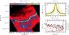 |
Fig. 7 Properties of a filament in the field G163.82-8.44. The frame a) shows the column density map. The white line shows the filament that was originally traced by eye and the yellow line follows the ridge that is formed by the peaks of the column density profiles in the perpendicular direction. The black filled circle indicates the start of the examined filament section. The tick marks are drawn at 5 arcmin intervals. The frame b) shows the average column density profile of the filament (black line), as well as the Plummer profile (the red dashed line on top of the black line) that was fitted together with a linear baseline (the blue dashed line) over the range –0.4 pc to +0.4 pc. The yellow lines show individual column density profiles for 20% of the cuts with the highest column densities (values normalized to a peak value of one, the right hand scale). The frame c) shows the FWHM values (the black circles) and the parameter Rflat of the Plummer fit (the red crosses), and the column density along the ridge of the filament (the solid line and the right hand scale) as a function of the distance along the filament. With the estimated distance of 350 pc, the SPIRE 250 μm data resolution of 18″ corresponds to 0.03 pc. The plots for the other fields are shown in Appendix D. |
Properties of selected filaments.
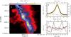 |
Fig. 8 The filament in the field G300.86-9.00 (PCC550) that is part of the Musca molecular cloud at the distance of 230 pc. See Fig. 7 for the details. |
3.2. Comparison with other infrared data
We have compared the sub-millimetre observations with the mid-infrared and far-infrared data from the WISE and AKARI satellites. The shorter wavelengths are more sensitive to temperature differences in the thin surface layers of the clouds and can trace variations in the heating radiation field or in the relative abundance of small and large grains (Laureijs et al. 1989; Bernard et al. 1992; Ridderstad & Juvela 2010). Therefore, these data can give further clues to the nature and the formation process of the clumps.
In addition to the SPIRE 250 μm data, Fig. 4 and the figures in Appendix A show the WISE 22 μm and the AKARI 90 μm, and 140 μm surface brightness maps. For example, the field G4.18+35.79 is apparently quiescent with no mid-infrared (MIR) or far-infrared (FIR) point sources (Fig. 4). On the other hand, in G130.37+11.26 (Fig. 5) the 22 μm data indicate clear star formation activity in connection with this mainly cold clump. The enhanced 22 μm emission towards the south further suggests an anisotropy of the radiation field. The lack of correlation or even clear anticorrelation between the PAH emission dominated MIR and the FIR/sub-mm emission is a feature repeated in many of the fields.
Figures 9 and C.1 show cross sections of the surface brightness data along the lines marked in frame b of Fig. 4 and the figures of Appendix A. The figures show the intensities after the subtraction of the values in the reference regions that were marked in Fig. 4 and the figures of Appendix A.
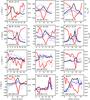 |
Fig. 9 Cross sections of the surface brightness data along the lines indicated in Figs. 4, 5 and in the figures of Appendix A. The lines show the 250 μm SPIRE data (thick black line), AKARI 140 μm and 90 μm data (solid and dashed blue lines), and, when available, the WISE 22 μm data (dotted line). The average surface brightness in the reference region (see Fig. 4b) has been subtracted from the plotted values. The red thick line is the colour temperature. The data have been convolved to the resolution of one arc minute. The 90 μm data have been scaled by a factor 20 and the 22 μm data by a factor of 600. When a different scaling has been used, the wavelength and the multiplicative scaling factor are given in the frame (λ:factor). The plots for the other fields are shown in Appendix C. |
3.2.1. Clump properties from dust emission
In this section we look in more detail at the properties of some major clumps, combining Herschel observations with the infrared data. The analysis uses the apertures that were marked in the frames a of Fig. 4 and figures in Appendix A.
The masses within the apertures were first determined using SPIRE data only. We derive two mass estimates. The first one is obtained by directly integrating over the aperture in the column density maps of Sect. 3.1.2. The spatial resolution of the column density maps is 40″. Because the column densities are calculated using the absolute surface brightness values, these should correspond to the total mass along the line of sight. However, the estimates are based on colour temperatures that, in the case of cold cores, can seriously overestimate the temperature inside the cores. We calculate another mass estimate using aperture photometry. The SPIRE surface brightness maps are convolved to a resolution of 40″. We measure the signal within the aperture and subtract the background using an annulus that extends to 1.5–2.0 times the radius of the aperture, thus removing most of the diffuse signal. The aperture sizes are listed in Table 2. The uncertainties of the flux values are derived from the surface brightness fluctuation in the annulus. The resulting SPIRE fluxes are fitted with a modified blackbody to estimate the clump masses. Because of the local background subtraction, these estimates should better reflect the temperature and the mass of the dense structures only. The mass estimates are listed in Table 2.
We have constructed the clump SEDs from 22 μm to the SPIRE wavelengths. Figure 10 shows the SEDs for clumps in the first twelve fields (in order of increasing Galactic longitude) and similar figures for the remaining fields can be found in Appendix E. In addition to the three SPIRE channels (250 μm, 350 μm, and 500 μm) the plots include the AKARI FIS bands (65 μm, 90 μm, 140 μm, and 160 μm) and the WISE data at 12 and 22 μm. The data were convolved to one arcmin resolution. The local background subtraction was performed as in the case of SPIRE data above, using an annulus around the aperture. Alternatively, because we do not have absolute surface brightness measurements in all infrared bands, the background can be estimated using the reference areas indicated in the frames b of Fig. 4 and in Appendix A. If the signal in the reference area is small, the resulting spectra should give a good estimate of the intensity and the spectral shape of the total emission along the line of sight. The data at wavelengths λ > 100 μm were fitted with modified blackbodies, Bν(T) νβ, with a fixed value of the emissivity spectral index, β = 2.0. The resulting colour temperatures are given in the figures.
We now have several colour temperature estimates for each aperture. Two are based on SPIRE only (as in Fig. 4 and Table 2) and two additionally include the AKARI 140 μm and 160 μm data (in Fig. 10 and Appendix E). Furthermore, in two cases we use the total surface brightness values (or an approximation obtained with the help of the reference areas) while in the other two cases the local background is subtracted using an annulus. The temperature estimates are compared in Fig. 11. The subtraction of the local background typically leads to ~2 K lower colour temperatures as expected for sources colder than their environment. The values are lowered by a further 1–2 K when the FIR data are included in the modified blackbody fits. One would have expected the temperatures to be lower when the shorter wavelengths are excluded (see Shetty et al. 2009b). The result could suggest a small difference in the calibration of the two instruments. The other possibility is that the FIR intensities are partly saturated. For the typical beam averaged peak column densities of 1022 cm-2, the 100 μm optical depth is of the order of 0.01, too little to cause noticeable effects. If the mass is concentrated to a very small area within the beam, the optical depths will be higher. A 1–2 K difference in the colour temperature would require column densities in excess of 1024 cm-2. Such values are possible, for example, in case of distant, pre-high-mass clumps. However, the optical depths are unlikely to be the main explanation for the whole sample because that would require that most of the mass within the beam is always concentrated on such high optical depth sightlines.
 |
Fig. 10 Spectral energy distributions for the apertures indicated in Fig. 4 and Appendix A. The plots include the 22 μm WISE data, the AKARI data at 65 μm, 90 μm, 140 μm, and 160 μm, and the three SPIRE channels at 250 μm, 350 μm, and 500 μm. In most fields two aperture positions were chosen and the data for the second one are shown in red. The background subtraction was done using the reference areas marked in Figs. 4 and the figures of Appendix A (solid symbols) or by using a local annulus (open symbols). The colour temperatures from the modified blackbody fits with β = 2 are listed in the frames. Plots for the other fields can be found in Appendix E. |
3.2.2. Search for coreshine
Steinacker et al. (2010) detected enhanced mid-infrared surface brightness in the Spitzer/IRAC 3.6 and 4.5 μm channels towards the cloud LDN 183. The high intensity of the 3.6 μm band relative to the 4.5 μm band, the absence of emission in the 5.8 μm band, the presence of absorption in the 8 μm band, and other considerations, led them to the conclusion that neither PAHs nor warm grains could explain these observations which were interpreted as a sign of enhanced light scattering caused by an increase in the size of the dust grains. This excess, named by the authors as coreshine, would thus serve as a tracer of the grain evolution, similar to the increase of the sub-millimetre dust opacity (e.g. Stepnik et al. 2003; Planck Collaboration 2011a). Thus, this phenomenon could also be used as an indicator of the evolutionary stage of our clumps. We examined the correlation between the WISE satellite 3.4, 4.6, and 12 μm bands and the 250 μm band measurements from SPIRE. If the grain size has indeed significantly increased, the WISE 3.4 μm band should include an additional component of scattered light that makes it brighter than expected compared to its surroundings and this should be correlated with the absence of emission, or better the absorption in the WISE 12 μm band, weaker or no emission in the WISE 4.6 μm band and these features should appear inside the 250 μm emission region.
The 4.6 μm band includes H2 lines that can be strong in outflows (Cyganowski et al. 2011). Also the 3.4 μm band is affected by H2 emission but, for typical excitation conditions, the intensity is much lower than in the 4.6 μm band (Reach et al. 2006). Furthermore, the H2 emission is also seen in the next MIR bands (5.8 μm and 8 μm for Spitzer/IRAC and 12 μm for WISE) and is therefore easy to distinguish from coreshine for which absorption is expected at these longer wavelengths.
One caveat concerns the absorption of the MIR radiation from the sky behind the source. Because the cloud opacity increases towards the shorter wavelengths, the background radiation is attenuated more at 3.4 μm than at 4.6 μm. If the background level is high, the detection of the coreshine may require modelling of the absorption and emission processes. This suggests that the direct effect is best seen at high Galactic latitudes where the sky brightness is low. This has been remarked by Pagani et al. (2010) who could find no cases of coreshine emission in the galactic plane itself. An upper limit of 0.37 MJy sr-1 in the background brightness level (which is linked to the density of the field stars) to allow for coreshine detection has been derived and will be discussed elsewhere (Pagani et al., in prep.). Another limitation comes from the low resolution of the WISE satellite (6.1′′ for all three bands, 3.4, 4.6 and 12 μm), which, combined with a high density of stars close to the galactic plane, tends to fill up the space with starlight, hiding possible coreshine effects. Figure 12 shows data for the field G6.03+36.73 (LDN183), one of the strongest coreshine detections, already discussed by Steinacker et al. (2010). The central filament, as traced by the 250 μm emission, is clearly visible in the 3.4 μm map. There is clear detection in emission at 4.6 μm and in absorption at 12 μm. The coreshine intensity is comparable to the one reported by Steinacker et al. (2010). The 3.4 μm signal increase is larger than for the 4.6 μm one and the cross-sections of the surface brightness show that the increase of the 3.4 μm/4.6 μm ratio is correlated with both the 250 μm emission and the decrease of the dust temperature.
We have similarly examined the 3.4, 4.6 and 12 μm images of all the 56 fields for which public WISE data are available. We compare them with the 250 μm SPIRE surface brightness maps that act as a tracer of the large grains. Figure 13 shows another example of detected coreshine.
4. Discussion
4.1. The nature of the observed fields
The observations show that the clouds associated with cold clumps have varied morphologies. The cloud sizes range from nearby globules ~0.2 pc to massive filaments more than 20 pc in length. With very few exceptions, the clumps exhibit a significant amount of sub-structure down to the resolution limit (0.01 pc for the nearest regions, over 0.2 pc for the most distant ones).
Of the 71 fields examined, 36 fields or 51% were categorized as having a clear filamentary structure. The definition of a “filament” here applies to the major structures but is taken in a widest possible sense, meaning anything from slightly elongated structures (e.g., G1.94+6.07 or G10.20+2.39) to the very long and narrow ‘real’ filaments like those observed in the fields G82.65-2.00 and G276.78+1.75. Several filaments appear to have formed, or at least significantly deformed, by some external force. This is visible as an asymmetry or a sharp drop in the spatial distribution of emission and column density (e.g., G25.86+6.22, G94.15+6.50, G130.37+11.26, or G315.88-21.44, see Figs. A.7, A.18, 5, and A.65). Thus, the origin of these filamentary structures could be different, i.e., turbulence vs. direct compression by radiation or pressure waves. This could be reflected in their properties which are further discussed in Sect. 4.3. However, further study of the interaction with, e.g., nearby HII regions is deferred to a future paper.
Altogether eight fields showed features reminiscent of compression by an external force (marked with “B” in Col. 8 of Table 1) that has lead to a sharp boundary visible in the column density maps. Such an interaction can also manifest itself at larger scales, as a cometary of a filamentary shape of the entire cloud. This sample includes some well known cometary shaped clouds (e.g., LDN 1780). At low resolution, the cloud LDN1340 (field G130.37+11.26) also looks like a classic cometary cloud but at higher resolution is found to consist of an intricate network of filaments that, particularly in the tail of the cloud, breaks down to many smaller clumps.
The clumps with a simple structure are mostly nearby objects where the spatial resolution allows us to resolve the core scales. However, there also are some more distant objects in this category. The target G39.65+1.75 is at a distance of 1.8 kpc and it is probable that it would not be such a featureless “blob” if it could be better resolved. On the other hand, the main clump in G26.34+8.65 is resolved but shows remarkably little structure for such a distant and therefore large object. However, one must keep in mind that the distance estimates of some of the objects are still quite uncertain and the distances of objects like G26.34+8.65 might be overestimated.
The colour temperature maps (Figs. 4, 5 and Appendix A) show that the dense structures are, in colour temperature, typically 2–3 degrees colder than their diffuse environment. The appearance of the temperature maps, i.e. their strongly spatially correlated values, indicates that the maps are dominated by real temperature variations rather than noise. The analysis of the uncertainties suggested that in the temperature maps the relative values are quite reliable (Sect. 3.1.1) although calibration errors could cause a shift of about ± 1 K (see Sect. 3.2.1).
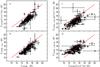 |
Fig. 11 Comparison of the temperature estimates for the selected clumps. In the left hand frames, the x-axis is the temperature derived from the total surface brightness. This is correlated with the minimum values within the apertures (frame b) and the values obtained with a local background subtraction (frame a). In the right hand frames the SPIRE temperatures (with background subtraction) are compared with the values obtained using the combination of SPIRE and AKARI data (λ > 100 μm) and with (frame c) or without (frame d) the subtraction of the local background. |
The colour temperature calculations were based on the use of a fixed value of the dust emissivity spectral index, β. There is evidence that, at least statistically, there exists an inverse relation between the observed spectral index and the dust temperature (Dupac et al. 2003; Désert et al. 2008; Planck Collaboration 2011c; Veneziani et al. 2010; Paradis et al. 2010). It is still debated to what extent this is caused by the intrinsic dust properties, by the line-of-sight temperature variations (Shetty et al. 2009b; Malinen et al. 2011; Juvela & Ysard 2012a; Ysard et al. 2012), and, in particular, by the noise that is known to produce some anticorrelation between the colour temperature and the spectral index (Shetty et al. 2009a; Juvela & Ysard 2012b). However, the anticorrelation appears to be an established observational fact and stronger than what is produced by the noise only (Planck Collaboration 2011c). If the average spectral index is larger in cold regions, the temperature contrasts (i.e., the difference in derived colour temperature) would be higher than indicated by our maps. Figure 14 shows some spectra consistent with the relation β(T) = (δ + ωT)-1 with parameters δ = 0.02 and ω = 0.035 as estimated from the analysis of Planck observations of dense cores (Planck Collaboration 2011c). The relative intensities in the SPIRE channels and the SED fits obtained with a fixed value of β = 2.0 are shown. For example, when a value of β = 2.0 is assumed, the estimated colour temperature is 12.2 K while the actual values of the spectral index and temperature are β = 2.7 and Tdust = 10 K. The figure also illustrates that, without further far-infrared data, simultaneous determination of colour temperature and spectral index is not possible.
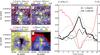 |
Fig. 12 Evidence of coreshine in the field G6.03+36.73 (LDN 183). Shown are the WISE 3.4 μm, 4.6 μm, and 12 μm WISE maps (frames a–c) and the SPIRE 250 μm map (frame d). Frame e) shows surface brightness profiles along the arrow marked in the previous frames. The lines correspond to the 3.4 μm (solid line), 4.6 μm (dashed line), 12 μm (dash-dotted line), and 250 μm data (dotted line). The numbers in the upper right corner give the possible scaling applied to the data before plotting (λ:factor). The red line and the right hand scale show the colour temperature. |
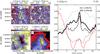 |
Fig. 13 Evidence of coreshine in the field G4.18+35.79 (LDN 134). See Fig. 12 for a description of the figure. |
We conclude that the colour temperature maps do reliably identify the coldest clumps although the absolute temperature values may be uncertain up to a couple of degrees. The real dust temperature inside the clumps cannot be directly measured and could be estimated only by modelling. From earlier theoretical studies, it is clear that in many cases the central temperature of the dense cores goes below 10 K (e.g., Evans et al. 2001; Harju et al. 2008). In particular, in LDN 183, our field G6.03+36.73, Pagani et al. (2004) reported dust temperatures down to ~7 K. In the dense and cold environment the dust grains are expected to undergo coagulation that can lead to increased opacity at sub-millimetre wavelengths (Ossenkopf 1993; Stepnik et al. 2003; Ysard et al. 2012; Köhler & et al. 2012). At the same time, the abundance of small grains should decrease, leading to lower mid-infrared emission. Examination of the data for the apertures shown in the figures of Appendix A revealed no significant anticorrelation between the surface brightness ratio 22 μm/90 μm and the ratio 90 μm/250 μm or the colour temperature measured in the wavelength range 250–500 μm. There could be several reasons for this. Firstly, most clumps could be too young so that the coagulation process, which may take millions of years, has not had time to alter the abundance of the small grains (Ossenkopf & Henning 1994; Chakrabarti & McKee 2005). Another natural reason is that the 22 μm emission comes mainly from a region with AV < 2m, as indicated by MIR limb brightening in radiative transfer models (Bernard et al. 1992; Fischera & Dopita 2008), and thus is not sensitive to processes deep inside the cores. The IR point sources associated with the cold clumps are another complication. Many regions are already forming stars so that the MIR data, the 22 μm band included, are dominated by the warm sources rather than the extended dust emission. This contaminates the correlations between MIR emission and the mean colour temperature of the large grains.
In a few individual clumps, an anticorrelation does exist between the column density, as traced by the sub-millimetre emission, and the MIR emission. These include the fields G6.0+36.7, G37.49+3.03, and G26.34+8.65 as shown in Fig. 9 and some further examples can be seen in Appendix C.
4.2. Connection with star formation
Star formation activity is visible in the MIR maps as sources spatially correlated to the cold dust emission. The best example is the field G216.76-2.58 where ten strong WISE MIR sources are detected along the high column density structures. This does not prevent cold dust being detected at longer wavelengths in exactly the same areas, with colour temperatures down to Tdust ~ 12 K. As a preliminary quantitative estimate of the star formation activity we counted the surface density of MIR sources. For each field for which WISE data were available, we made a list of the 22 μm point sources. The detection was done with the SExtractor program, excluding sources that are significantly more extended than the beam (FWHM larger than 10 pixels = 60″). Each field was divided into a low and a high column density part using the median column density as the dividing value. The source densities were calculated for the two parts. Figure 15 shows the source density in the high column density areas (i.e., sources likely to be associated with the clumps) relative to the average source density in the field.
The interpretation of such correlations is not straightforward. The youngest objects should reside within the areas of high column density and thus lead to a positive correlation (fields on the right hand side of Fig. 15). A negative correlation could appear in more evolved regions where the sources have cleared their surroundings. However, with the typical clump column densities of 1022 cm-2 (AV ~ 10), the 22 μm optical depth approaches unity and this is enough to affect the number density of the detected background sources. Therefore, the fields in the left hand part of Fig. 15 could represent either cases without associated star formation or cases with a larger number of background sources. The number of MIR sources and the correlations may be further affected by the source distances because of the sensitivity limit of the WISE survey. However, the overall source densities of the fields and the fraction of sources in the high column density areas do not appear to be correlated (see Fig. 15).
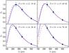 |
Fig. 14 Spectral energy distributions (solid curves) for 10, 13, 16, and 19 K colour temperatures assuming the β(T) relation given in Planck Collaboration (2011c). The corresponding values at the SPIRE wavelengths are plotted with 10% error bars. The dashed lines show the spectra fitted to these data points assuming β = 2.0. The corresponding temperature values are quoted after the arrows. |
About 50 percent of the clumps are located on FIR loops (Könyves et al. 2007) that are boundary regions (shells) around the voids in the galactic ISM. A preliminary analysis of a sample of sources and their AKARI FIR photometry showed that the clumps located on the shells have ~20% higher probability of being associated with YSO candidates (Marton 2012). In particular, a detailed analysis of the 62 IR point sources in the “snake” cloud (California nebula, G163.82-8.44) region resulted in a number of YSO candidates. The sources were analysed using the AKARI IRC and FIS (Ishihara et al. 2010; Murakami et al. 2007; Yamamura et al. 2010), the 2MASS and IRAS point source catalogues, as well as optical photometry data available in public archives. On the basis of the physical parameters derived for the sources, there are 11 low-mass and 2 intermediate mass young stellar objects in evolutionary phases ranging from Class 0/I to Class III. In that particular field, the estimated ages suggest that the star formation started several million years ago and is still on-going. Further details will be given in a separate paper (Zahorecz et al., in prep.).
4.3. Filamentary structures
4.3.1. The uncertainties of filament analysis
The characterisation of the filaments depends on the way the analysed structures are selected and on the analysis methods themselves. We selected at most one elongated structure from each field. One should consult the figures in Appendix D to check to what extent these correspond to ones own conception of filaments. There are automatic routines for the detection of filaments, for example the DisPerSE routine (Sousbie 2011) used in Arzoumanian et al. (2011) and Hill et al. (2011). We chose to do the selection manually, limiting the analysis to the main structures. Once these have been selected, we followed the ridge of the filament, connecting the column density peaks sampled at 20″ intervals. Unless the filament has a very well defined, smooth ridge, this decision affects the derived filament widths. The structures are often fragmented and the column density peaks do not necessarily follow a single line. If one draws a wiggly filament through every individual clump, one is measuring the sizes of those smaller structures. One could equally describe the system as a more straight filament, allowing the spatial scatter of the substructures to be counted as part of its width. Another critical parameter is the spatial extent analysed. For the FWHM values the effect is obvious and the values increase with the size of the analysed area, i.e., with the maximum distance from the centre of the filament. This is caused by the hierarchical structure of the ISM and the need to apply background subtraction at some scale to remove the contribution of extended emission that is not directly connected with the filament. The fit of the Plummer profile may be less affected, but only as far as the actual column density profile can be precisely fitted with that particular functional form. Because of these ambiguities, the width of the filament and its other parameters are not well defined and different studies can be compared only when the methods and the probed linear scales are identical. In particular, to be able to compare sources at different distances, we were forced to select ± 0.4 pc as the extent of the structures examined.
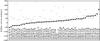 |
Fig. 15 The fields sorted in increasing number density of the 22 μm sources in the high column density areas relative to the average source density of the field. The circles are the excess of sources per square degree. The horizontal dashes show the total source density, including both the high and the low column density areas. |
There are several reasons why our dust observations may give an incomplete picture of the structure of the clouds. Firstly, the column density values may be biased in the presence of temperature variations that exist along the line of sight and within the beam. Because warm dust emits more strongly, the colour temperature overestimates the true, mass weighted dust temperature. Consequently, the column densities will be underestimated and the effect is most notable towards the centre of the filaments where the temperature variations along the line of sight are the largest. In our analysis of Sect. 3.1.4 we use column density maps that are based on lower, 40″ resolution colour temperature information. To quantify the associated biases, we examined radiative transfer models of cylinders with Plummer like density profile (Ysard et al. 2012). The dust temperature distributions were solved assuming that the cylinders are heated externally by an interstellar radiation field with intensity applicable to the solar neighbourhood (Mathis et al. 1983). The resulting synthetic surface brightness maps were analysed as the SPIRE observations, deriving colour temperature maps at the 40″ resolution and the column density maps at the 20″ resolution. The data were then fitted with Plummer functions and the obtained parameters were compared to the actual values of the column density distribution. For a filament ρC = 104 cm-3, Rflat = 0.58 pc, and p = 2.0, the correct parameters were recovered with an accuracy better than 10%, even when the source was moved to a 1 kpc distance and a 3% observational noise was added to the surface brightness values. The relative errors increase with the density of the filament, also because the density peak is less well resolved. With ρC = 106 cm-3, Rflat = 0.0055 pc, and p = 2.0, the parameter ρC was underestimated by ~30% and Rflat similarly overestimated by ~30% for a source at 100 pc. For a more distant target with (1 kpc), the typical error was a factor of three larger. The estimates of the parameter p still remain correct to within 30% in all the tests. The results suggest that the central density will be underestimated and the filament radius, Rflat, overestimated but, for the typical filaments in our sample, the errors are below 50%. In the tests the density of the filaments perfectly followed the Plummer profile. Therefore, it does not indicate if the results would be sensitive to small deviations from the Plummer shape such as, e.g., in the presence of asymmetries or substructure. However, it is clear that the ρC and Rflat parameters are intrinsically anticorrelated.
Further studies are required to find out how the combination of low resolution colour temperature and higher resolution surface brightness data compares with the normal procedure of convolving all data to the lowest common resolution.
4.3.2. Filament structure
The width of the filaments (or more generally, of the selected structures shown in Appendix D) were found to cover a large range from ~0.1pc to close to 1 parsec.
The FWHM widths are often larger than 0.1 pc and also vary along the length of the filaments. The width is often anticorrelated with the column density, the smallest FWHM values being associated with the highest column densities, i.e., dense clumps and cores. Part of this anticorrelation is caused by the non-continuous nature of some filaments where no real column density excess is detected between the clumps. Depending on the structure of the surrounding ISM, the widths obtained in the gaps between the clumps can be very large. However, there is also real anticorrelation that can be seen in fields like G300.86-9.00 (PCC550), G167.20-8.69, and G227.95-2.98.
The distances between denser cores can be as low as ~0.1 pc (e.g. G110.89-2.78) but are typically 0.5 pc or higher and thus significantly above the Jeans length. For example, G167.20-8.69 shows a very regular pattern with column density peaks at 0.6 pc intervals. The results are consistent with Henning et al. (2010) who measured a core separation of 0.9 pc in the infrared dark cloud filament G011.11-0.12.
Several fields are actively forming stars and many of the observed dense cores are likely to be gravitationally bound as discussed in Planck Collaboration (2011b). This strongly suggests that many of the mapped cores are undergoing gravitational collapse. However, anticorrelation between column density and filament width is expected even for isothermal gas cylinders in hydrostatic equilibrium. Similarly, when hydrostatic spherical clumps reside inside hydrostatic filaments, the former are likely to have smaller FWHM values. Figure 16 shows Plummer profiles and the column density profiles for Bonner-Ebert spheres with masses equal to the filament mass within one Jeans length (assuming T = 10 K). The cores are seen to have higher column densities and smaller FWHM values. Note that in this calculation, if the central density of the filament is very high, the peak column density of the corresponding Bonnor-Ebert sphere could remain lower because of the very short Jeans length. The figure also illustrates that if the filament profiles extend far beyond the 0.4 pc distance used in our analysis, the FWHM estimates (as opposed to the values obtained from the profile fits) will be biased toward lower values.
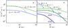 |
Fig. 16 Radial column density profiles of selected Plummer profile filaments (solid lines) and Bonnor-Ebert spheres (dashed lines). a) Two filaments with Rflat = 0.1 pc and p = 2 and a central density of ρc = 103 cm-3 or ρc = 5 × 103 cm-3, and a Bonner-Ebert sphere with a mass of 6.0 M⊙ that in both cases corresponds to the filament mass within one Jeans length. b) Filaments with a central density ρc = 103 cm-3 with values p/Rflat as indicated in the figure. The dashed lines are column density profiles for Bonnor-Ebert spheres with mass equal to the mass of the filaments within a distance of one Jeans length. |
A few sources (G89.65-7.02, G159.34+11.21, G176.27-2.09, G276.78+1.75) could not be fitted properly using the limited range of ±0.4 pc. In most cases this results from the fact that one is looking at some elongated structures whose basic nature is different from that of actual filaments. However, the fields G176.27-2.09 and G276.78+1.75 clearly do have the appearance of regular filaments while their widths are closer to 1 pc instead of the more typical ~0.2–0.3 pc. In both cases the estimated distances are large, ~2 kpc. This again raises the question whether these could in fact be more nearby clouds.
The widths of our filaments are on the average larger than those reported by Arzoumanian et al. (2011) for the filaments in IC5146. In some cases our structures might be further divided into smaller filaments, depending on the way the filament detection is performed (cf. Arzoumanian et al. 2011, Fig. 1). Thus, clouds can exhibit a hierarchical structure also regarding the filaments.
4.4. Coreshine
Out of the 56 fields examined for the presence of coreshine, 12 are too close to the galactic plane and show background emission above the threshold. They are not considered any further. At 12 μm, 9 fields showed (weak) emission (most probably linked to PAH emission), 13 fields were not detected and 22 showed absorption. Emission at 3.4 μm was found either in correlation with the emission at 12 μm (PAHs) and in a few cases in correlation with absorption at 12 μm (coreshine). Apart from the well-known L183 case (G6.03+36.73), coreshine was clearly identified in three other fields only, G4.18+35.79 (LDN134), G210.90-36.55 (LDN1642, MBM20-21) and G300.86-9.00 (PCC550, in the Musca Complex). LDN 134 was erroneously reported as showing no coreshine in Pagani et al. (2010). LDN 1780 (G358.96+36.75), the third cloud in the same complex as LDN134 and LDN183, is bright at 12 μm, unlike the two others and is therefore dominated by PAH emission. There are six additional fields with clumps showing possible signs of coreshine (G130.37+11.26, G167.20-8.69, G173.43-5.44, G181.84-18.46, G215.44-16.38, G298.31-13.05). However, the MIR intensity ratio is seen to have large variations that are not correlated with the dust column density (or the dust temperature). Therefore, these detections can be said to be only tentative. The sample also includes targets like G39.65+1.75 where the relative intensity of the 3.4 μm and 4.6 μm appears to be determined mainly by the extinction of background radiation. Most of the fields with tentative or positive coreshine detection are at high latitudes. Although not an absolute requirement, a low background surface brightness makes it easier to detect the faint MIR excess caused by the scattering. In many other medium to high latitude sources (e.g., G108.28+16.68, G212.07-15.21, G315.88-21.44) the results were negative or inconclusive. Finally, only 7 to 18% of the fields show confirmed or possible coreshine. This is markedly lower than the results reported by Pagani et al. (2010) with a ~50% detection rate.
It is not yet understood why some cores show the coreshine effect while others do not. Time is needed to let the grains grow but time is clearly not the only factor. A high peak column density also is not a necessary nor a sufficient criterion as coreshine is clearly detected towards sources with N(H2,peak) ≤ 1 × 1022 cm-2 and still not towards sources at similarly high latitude but with peak column densities 2–3 times as high. The low resolution of the WISE experiment is possibly a strong limitation, combined with the small extent of many of the clumps. The coreshine studies would benefit not only from higher spatial resolution but also from data with a higher signal-to-noise ratio. The Spitzer program Hunting coreshines with Spitzer (PI R. Paladini) is currently carrying out observations that, compared to the WISE data, will be more sensitive by a factor of ten. The targets of that survey, 90 in number, have been selected from the Planck Early Cold Cores Catalogue (ECC) and correspond to ~10% of the ECC. Detailed modelling is needed to separate the coreshine from the effects of the attenuation of the background radiation and to quantify the degree of the grain growth.
5. Conclusions
We have examined a sample of 71 fields that were mapped with the Herschel SPIRE instrument as part of the key programme Galactic cold cores. The examination of the sub-millimetre Herschel observations and the available AKARI and WISE infrared data leads to the following conclusions:
-
The data confirm the presence of cold dust with colourtemperatures of the total intensity typically going down to ~14 K or below. With the subtraction of the local background emission, the estimated temperature of the larger clumps can be at least 1–2 K lower, the effect being larger if one assumes that the dust emissivity spectral index in these regions rises above β = 2.0.
-
About 50% of the fields have a mainly filamentary structure, the filaments often being fragmented into a number of clumps. In several cases the morphology belies direct dynamic interaction, e.g., in the form of sharp interface layers. Several clearly cometary clouds are also seen, again combined with a significant amount of smaller scale structures.
-
The fields include a few quiescent clouds but most clouds show some signs of ongoing star formation. Young stellar objects, as detected in mid-infrared data, are found to co-exist with clumps having cold sub-millimetre spectra.
-
The mid-infrared data were searched for signs of coreshine, enhanced mid-infrared scattering potentially caused by the increased grain sizes. Clear signal was observed in four fields with a further six tentative detections.
-
The main filamentary structures found in the fields were analysed. The typical filament width was observed to be ~0.2–0.3 pc. The widths were anticorrelated with the column density, a behaviour expected both for isothermal, hydrostatic filaments of different densities and for gravitationally bound spherical cores embedded in filaments.
-
Statistically, no anticorrelation was found between the mid-infrared emission and the large grain temperature, as expected in the dust coagulation scenario. This can be explained by the fact that these wavelengths probe entirely separate parts of the clumps. On the other hand, several clumps were opaque enough to be seen as mid-infrared dark clouds, with a sharp decrease in the 22 μm surface brightness.
Online material
Appendix A: Maps of observed and derived quantities
Figures A.1–A.69 show maps of observed and derived quantities for the fields other than the one already shown in Figs. 4, 5. Included in the figures are the colour temperature map derived from SPIRE data (frame a, 40″ resolution), the 250 μm SPIRE surface brightness map (frame b, 18″ resolution), the AKARI wide filter maps at 140 μm and 90 μm (frames c and e; convolved to a resolution of one arc minute), the visual extinction AV derived from 2MASS catalogue stars (frame d; resolution of 2′), and the WISE 22 μm intensity (frame f; 12″ resolution). In the cases where public WISE data were not yet available, frame f shows the 25 μm IRAS map (resolution of 4.5′). The respective beam sizes are indicated in the lower right hand corner of each frame. The black circles indicate the positions of clumps selected for further examination in Sect. 3.2.1 and the white circles indicates a reference region used for background subtraction in the SED plots in Sect. 3.2.1. In frame a, the arrow indicates the position of the stripe plotted in Appendix C.
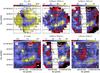 |
Fig. A.1 Data on the field G1.94+6.07. Shown are the colour temperature map derived from SPIRE data (frame a, 40″ resolution), the 250 μm SPIRE surface brightness map (frame b, 18″ resolution), the AKARI wide filter maps at 140 μm and 90 μm (frames c and e), the visual extinction AV derived from 2MASS catalog stars (frame d), and the WISE 22 μm intensity (frame f). In the subsequent figures, if public WISE data are not available, frame f shows the 25 μm IRAS map instead. The respective beam sizes are indicated in the lower right hand corner of each frame. The positions of selected clumps (black circles; see Sect. 3.2.1) and the reference regions used for background subtraction (white circle; see Sect. 3.2.1) are also shown. |
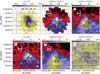 |
Fig. A.2 Data on the field G6.03+36.73. |
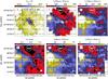 |
Fig. A.3 Data on the field G10.20+2.39. |
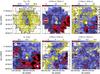 |
Fig. A.4 Data on the field G20.72+7.07. |
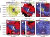 |
Fig. A.5 Data on the field G21.26+12.11. |
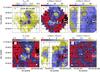 |
Fig. A.6 Data on the field G24.40+4.68. |
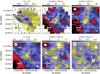 |
Fig. A.7 Data on the field G25.86+6.22. |
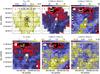 |
Fig. A.8 Data on the field G26.34+8.65. |
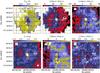 |
Fig. A.9 Data on the field G37.49+3.03. |
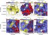 |
Fig. A.10 Data on the field G39.65+1.75. |
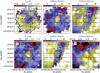 |
Fig. A.11 Data on the field G62.16-2.92. |
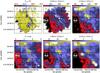 |
Fig. A.12 Data on the field G69.57-1.74. |
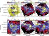 |
Fig. A.13 Data on the field G70.10-1.69. |
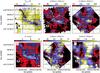 |
Fig. A.14 Data on the field G82.65-2.00. |
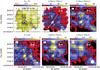 |
Fig. A.15 Data on the field G86.97-4.06. |
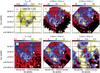 |
Fig. A.16 Data on the field G89.65-7.02. |
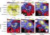 |
Fig. A.17 Data on the field G93.21+9.55. |
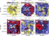 |
Fig. A.18 Data on the field G94.15+6.50. |
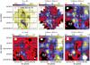 |
Fig. A.19 Data on the field G98.00+8.75. |
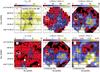 |
Fig. A.20 Data on the field G105.57+10.39. |
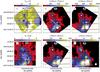 |
Fig. A.21 Data on the field G107.20+5.52 (PCC249). |
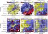 |
Fig. A.22 Data on the field G108.28+16.68. |
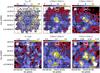 |
Fig. A.23 Data on the field G109.18-37.59. |
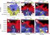 |
Fig. A.24 Data on the field G109.80+2.70 (PCC288). |
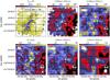 |
Fig. A.25 Data on the field G110.89-2.78. |
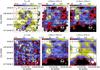 |
Fig. A.26 Data on the field G111.41-2.95. |
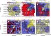 |
Fig. A.27 Data on the field G126.63+24.55. |
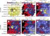 |
Fig. A.28 Data on the field G127.79+2.66. |
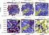 |
Fig. A.29 Data on the field G130.42-47.07. |
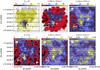 |
Fig. A.30 Data on the field G131.65+9.75. |
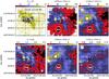 |
Fig. A.31 Data on the field G132.12+8.95. |
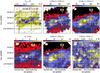 |
Fig. A.32 Data on the field G149.67+3.56. |
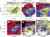 |
Fig. A.33 Data on the field G150.47+3.93. |
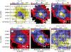 |
Fig. A.34 Data on the field G151.45+3.95. |
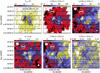 |
Fig. A.35 Data on the field G154.08+5.23. |
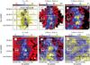 |
Fig. A.36 Data on the field G157.08-8.68. |
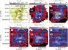 |
Fig. A.37 Data on the field G157.92-2.28. |
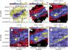 |
Fig. A.38 Data on the field G159.34+11.21. |
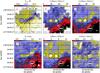 |
Fig. A.39 Data on the field G161.55-9.30. |
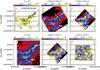 |
Fig. A.40 Data on the field G163.82-8.44. |
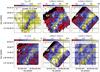 |
Fig. A.41 Data on the field G164.71-5.64. |
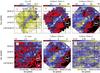 |
Fig. A.42 Data on the field G167.20-8.69. |
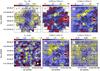 |
Fig. A.43 Data on the field G168.85-10.19. |
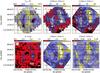 |
Fig. A.44 Data on the field G173.43-5.44. |
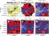 |
Fig. A.45 Data on the field G176.27-2.09. |
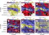 |
Fig. A.46 Data on the field G181.84-18.46. |
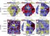 |
Fig. A.47 Data on the field G188.24-12.97. |
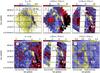 |
Fig. A.48 Data on the field G189.51-10.41. |
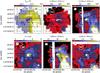 |
Fig. A.49 Data on the field G195.74-2.29. |
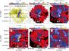 |
Fig. A.50 Data on the field G198.58-9.10. |
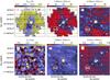 |
Fig. A.51 Data on the field G202.23-3.38. |
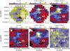 |
Fig. A.52 Data on the field G203.42-8.29. |
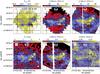 |
Fig. A.53 Data on the field G205.06-6.04. |
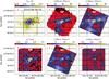 |
Fig. A.54 Data on the field G210.90-36.55. |
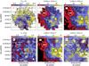 |
Fig. A.55 Data on the field G212.07-15.21. |
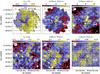 |
Fig. A.56 Data on the field G215.37-3.04. |
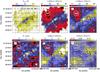 |
Fig. A.57 Data on the field G215.44-16.38. |
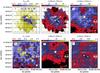 |
Fig. A.58 Data on the field G216.76-2.58. |
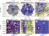 |
Fig. A.59 Data on the field G218.06+2.12. |
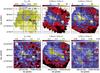 |
Fig. A.60 Data on the field G227.95-2.98. |
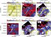 |
Fig. A.61 Data on the field G276.78+1.75. |
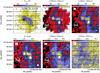 |
Fig. A.62 Data on the field G298.31-13.05. |
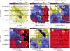 |
Fig. A.63 Data on the field G300.61-3.13. |
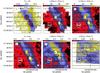 |
Fig. A.64 Data on the field G300.86-9.00 (PCC550). |
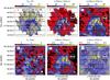 |
Fig. A.65 Data on the field G315.88-21.44. |
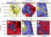 |
Fig. A.66 Data on the field G334.65+2.67. |
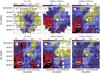 |
Fig. A.67 Data on the field G339.22-6.02. |
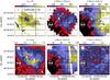 |
Fig. A.68 Data on the field G343.64-2.31. |
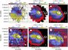 |
Fig. A.69 Data on the field G358.96+36.75. |
Appendix B: Column density maps
Figure B.1 shows the column density maps for all the fields excluding those already shown in Fig. 6.
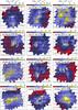 |
Fig. B.1 continued. |
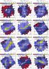 |
Fig. B.1 continued. |
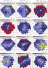 |
Fig. B.1 continued. |
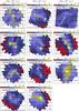 |
Fig. B.1 continued. |
Appendix C: One-dimensional cuts of the surface brightness data
Figure C.1 shows selected surface brightness values along the one-dimensional cuts marked in the frames a of Fig. 4 and Figs. A.1–A.69.
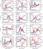 |
Fig. C.1 Cross sections of the surface brightness data along the lines indicated in Figs. 4, 5 and in the figures of Appendix A. The lines show the 250 μm SPIRE data (thick black line), AKARI 140 μm and 90 μm data (solid and dashed blue lines), and, when available, the WISE 22 μm data (dotted line). The average surface brightness in the reference region has been subtracted from the plotted values. The red thick line is the colour temperature. The data have been convolved to the resolution of one arc minute. The 90 μm data have been scaled by a factor 20 and the 22 μm data by a factor of 600. When a different scaling has been used, the wavelength and the multiplicative scaling factor are given in the frame (λ:factor). |
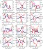 |
Fig. C.1 continued. |
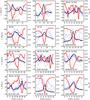 |
Fig. C.1 continued. |
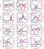 |
Fig. C.1 continued. |
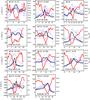 |
Fig. C.1 continued. |
Appendix D: Figures of the selected elongated cloud structures
The analysis of the filamentS in the fields G163.82-8.44 and G300.86-9.00 (PCC 550) were shown in Figs. 7, 8. The plots for the other fields listed in Table 3 are shown in Figs. D.1–D.24. These include only the fields with an existing distance estimate and where a clear filament or other distinct elongated structure could be discerned.
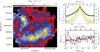 |
Fig. D.1 Properties of a filament in the field G1.94+6.07. The frame a shows the column density map. The white line shows the filament that was originally traced by eye and the yellow line follows the ridge that is formed by the peaks of the column density profiles in the perpendicular direction. The black filled circle indicates the start of the examined filament section. The tick marks are drawn at 5 arcmin intervals. The frame b shows the average column density profile of the filament (black line), as well as the Plummer profile (the red dashed line on top of the black line) that was fitted together with a linear baseline (the blue dashed line) over the range −0.4 pc to +0.4 pc. The yellow lines show individual column density profiles for 20% of the cuts with the highest column densities (values normalized to a peak value of one, the right hand scale). The frame c shows the FWHM values (the black circles) and the parameter Rflat of the Plummer fit (the red crosses), and the column density along the ridge of the filament (the solid line and the right hand scale) as a function of the distance along the filament. |
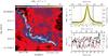 |
Fig. D.2 The filament selected from the field G82.65-2.00. |
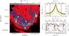 |
Fig. D.3 The filament selected from the field G89.65-7.02. |
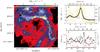 |
Fig. D.4 The filament selected from the field G94.15+6.50. |
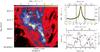 |
Fig. D.5 The filament selected from the field G98.00+8.75. |
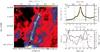 |
Fig. D.6 The filament selected from the field G105.57+10.39. |
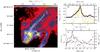 |
Fig. D.7 The filament selected from the field G126.63+24.55. |
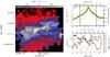 |
Fig. D.8 The filament selected from the field G149.67+3.56. |
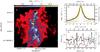 |
Fig. D.9 The filament selected from the field G157.08-8.68. |
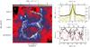 |
Fig. D.10 The filament selected from the field G157.92-2.28. |
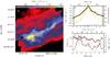 |
Fig. D.11 The filament selected from the field G159.34+11.21. |
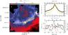 |
Fig. D.12 The filament selected from the field G161.55-9.30. |
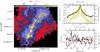 |
Fig. D.13 The filament selected from the field G164.71-5.64. |
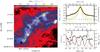 |
Fig. D.14 The filament selected from the field G167.20-8.69. |
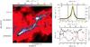 |
Fig. D.15 The filament selected from the field G176.27-2.09. |
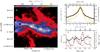 |
Fig. D.16 The filament selected from the field G181.84-18.46. |
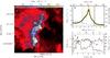 |
Fig. D.17 The filament selected from the field G198.58-9.10. |
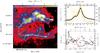 |
Fig. D.18 The filament selected from the field G203.42-8.29. |
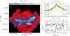 |
Fig. D.19 The filament selected from the field G205.06-6.04. |
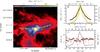 |
Fig. D.20 The filament selected from the field G210.90-36.55. |
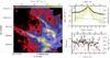 |
Fig. D.21 The filament selected from the field G212.07-15.21. |
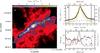 |
Fig. D.22 The filament selected from the field G215.44-16.38. |
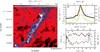 |
Fig. D.23 The filament selected from the field G276.78+1.75. |
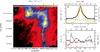 |
Fig. D.24 The filament selected from the field G298.31-13.05. |
Appendix E: Spectra of selected regions
The spectral energy distributions of selected regions were presented in Fig. 10. Similar figures for the remaining fields are shown in Fig. E.1.
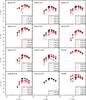 |
Fig. E.1 Spectral energy distributions corresponding to the apertures marked in the figures of Appendix A. The plots include 22 μm WISE data, AKARI data at 65 μm, 90 μm, 140 μm, and 160 μm, and the three SPIRE channels at 250 μm, 350 μm, and 500 μm. In most fields two aperture positions were chosen and the data for the second one are shown in red. The background subtraction was done using the reference areas marked in the figures of Appendix A (solid symbols) or by using a local annulus (open symbols). The colour temperatures from the modified blackbody fits with β = 2 are listed in the frames. |
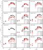 |
Fig. E.1 continued. |
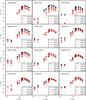 |
Fig. E.1 continued. |
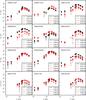 |
Fig. E.1 continued. |
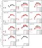 |
Fig. E.1 continued. |
SPIRE has been developed by a consortium of institutes led by Cardiff University (UK) and including Univ. Lethbridge (Canada); NAOC (China); CEA, LAM (France); IFSI, Univ. Padua (Italy); IAC (Spain); Stockholm Observatory (Sweden); Imperial College London, RAL, UCL-MSSL, UKATC, Univ. Sussex (UK); and Caltech, JPL, NHSC, Univ. Colorado (USA). This development has been supported by national funding agencies: CSA (Canada); NAOC (China); CEA, CNES, CNRS (France); ASI (Italy); MCINN (Spain); SNSB (Sweden); STFC (UK); and NASA (USA).
HIPE is a joint development by the Herschel Science Ground Segment Consortium, consisting of ESA, the NASA Herschel Science Center, and the HIFI, PACS and SPIRE consortia.
The reduced data will become available through the ESA web site http://herschel.esac.esa.int/UserReducedData.shtml. Further information is available on the home page of the Cold Cores project https://wiki.helsinki.fi/display/PlanckHerschel/The+Cold+Cores
SPIRE Observer’s manual, http://herschel.esac.esa.int/Documentation.shtml
Acknowledgments
M.J., J.M. and N.Y. acknowledge the support of the Academy of Finland Grants Nos. 127015 and 250741. N.Y. acknowledges the support of a CNES post-doctoral research grant. This publication makes use of data products from the Two Micron All Sky Survey, which is a joint project of the University of Massachusetts and the Infrared Processing and Analysis Center/California Institute of Technology, funded by the National Aeronautics and Space Administration and the National Science Foundation. This research is based in part on observations with AKARI, a JAXA project with the participation of ESA.
References
- André, P., Men’shchikov, A., Bontemps, S., et al. 2010, A&A, 518, L102 [NASA ADS] [CrossRef] [EDP Sciences] [Google Scholar]
- Arzoumanian, D., André, P., Didelon, P., et al. 2011, A&A, 529, L6 [Google Scholar]
- Beckwith, S. V. W., Sargent, A. I., Chini, R. S., & Guesten, R. 1990, AJ, 99, 924 [NASA ADS] [CrossRef] [Google Scholar]
- Bernard, J. P., Boulanger, F., Desert, F. X., & Puget, J. L. 1992, A&A, 263, 258 [NASA ADS] [Google Scholar]
- Boulanger, F., Abergel, A., Bernard, J., et al. 1996, A&A, 312, 256 [NASA ADS] [Google Scholar]
- Chakrabarti, S., & McKee, C. F. 2005, ApJ, 631, 792 [NASA ADS] [CrossRef] [Google Scholar]
- Cutri, R. M., Wright, E. L., Conrow, T., et al. 2011, Explanatory Supplement to the WISE Preliminary Data Release Products, Tech. Rep. [Google Scholar]
- Cyganowski, C. J., Brogan, C. L., Hunter, T. R., Churchwell, E., & Zhang, Q. 2011, ApJ, 729, 124 [NASA ADS] [CrossRef] [Google Scholar]
- Dame, T., Hartmann, D., & Thaddeus, P. 2001, ApJ, 547, 792 [NASA ADS] [CrossRef] [Google Scholar]
- Désert, F., Macías-Pérez, J. F., Mayet, F., et al. 2008, A&A, 481, 411 [NASA ADS] [CrossRef] [EDP Sciences] [Google Scholar]
- Dupac, X., Bernard, J., Boudet, N., et al. 2003, A&A, 404, L11 [NASA ADS] [CrossRef] [EDP Sciences] [Google Scholar]
- Elmegreen, B. G. 2011, ApJ, 731, 61 [NASA ADS] [CrossRef] [Google Scholar]
- Evans, II, N. J., Rawlings, J. M. C., Shirley, Y. L., & Mundy, L. G. 2001, ApJ, 557, 193 [NASA ADS] [CrossRef] [Google Scholar]
- Fischera, J., & Dopita, M. A. 2008, ApJS, 176, 164 [NASA ADS] [CrossRef] [Google Scholar]
- Fukui, Y., Mizuno, N., Yamaguchi, R., et al. 1999, PASJ, 51, 745 [NASA ADS] [CrossRef] [Google Scholar]
- Goldsmith, P. F. 2001, ApJ, 557, 736 [NASA ADS] [CrossRef] [MathSciNet] [Google Scholar]
- Griffin, M. J., Abergel, A., Abreu, A., et al. 2010, A&A, 518, L3 [Google Scholar]
- Harju, J., Juvela, M., Schlemmer, S., et al. 2008, A&A, 482, 535 [NASA ADS] [CrossRef] [EDP Sciences] [Google Scholar]
- Hawarden, T. G., & Brand, P. W. J. L. 1976, MNRAS, 175, 19P [NASA ADS] [CrossRef] [Google Scholar]
- Henning, T., Linz, H., Krause, O., et al. 2010, A&A, 518, L95 [NASA ADS] [CrossRef] [EDP Sciences] [Google Scholar]
- Hill, T., Motte, F., Didelon, P., et al. 2011, A&A, 533, A94 [NASA ADS] [CrossRef] [EDP Sciences] [Google Scholar]
- Ishihara, D., Onaka, T., Kataza, H., et al. 2010, A&A, 514, A1 [NASA ADS] [CrossRef] [EDP Sciences] [Google Scholar]
- Juvela, M., & Ysard, N. 2011, ApJ, 739, 63 [NASA ADS] [CrossRef] [Google Scholar]
- Juvela, M., & Ysard, N. 2012a, A&A, 539, A71 [NASA ADS] [CrossRef] [EDP Sciences] [Google Scholar]
- Juvela, M., & Ysard, N. 2012b, A&A, in press, DOI: 10.1051/0004-6361/201118596 [Google Scholar]
- Juvela, M., Ristorcelli, I., Montier, L. A., et al. 2010, A&A, 518, L93 [NASA ADS] [CrossRef] [EDP Sciences] [Google Scholar]
- Juvela, M., Ristorcelli, I., Pelkonen, V.-M., et al. 2011, A&A, 527, A111 [NASA ADS] [CrossRef] [EDP Sciences] [Google Scholar]
- Köhler, M., et al. 2012, A&A, submitted [Google Scholar]
- Könyves, V., Kiss, C., Moór, A., Kiss, Z. T., & Tóth, L. V. 2007, A&A, 463, 1227 [NASA ADS] [CrossRef] [EDP Sciences] [Google Scholar]
- Kramer, C., Richer, J., Mookerjea, B., Alves, J., & Lada, C. 2003, A&A, 399, 1073 [NASA ADS] [CrossRef] [EDP Sciences] [Google Scholar]
- Laureijs, R. J., Chlewicki, G., Wesselius, P. R., & Clark, F. O. 1989, A&A, 220, 226 [NASA ADS] [Google Scholar]
- Lehtinen, K., Russeil, D., Juvela, M., Mattila, K., & Lemke, D. 2004, A&A, 423, 975 [NASA ADS] [CrossRef] [EDP Sciences] [Google Scholar]
- Lehtinen, K., Juvela, M., Mattila, K., Lemke, D., & Russeil, D. 2007, A&A, 466, 969 [NASA ADS] [CrossRef] [EDP Sciences] [Google Scholar]
- Lombardi, M., & Alves, J. 2001, A&A, 377, 1023 [NASA ADS] [CrossRef] [EDP Sciences] [Google Scholar]
- Malinen, J., Juvela, M., Collins, D. C., Lunttila, T., & Padoan, P. 2011, A&A, 530, A101 [NASA ADS] [CrossRef] [EDP Sciences] [Google Scholar]
- Marshall, D. J., Joncas, G., & Jones, A. P. 2009, ApJ, 706, 727 [NASA ADS] [CrossRef] [Google Scholar]
- Martin, P. G., Roy, A., Bontemps, S., et al. 2012, ApJ, in press [arXiv:1112.5433] [Google Scholar]
- Marton, G. 2012, Ph.D. Thesis, Eötvös University, Budapest [Google Scholar]
- Mathis, J. S., Mezger, P. G., & Panagia, N. 1983, A&A, 128, 212 [NASA ADS] [Google Scholar]
- McKee, C. F., & Ostriker, E. C. 2007, ARA&A, 45, 565 [NASA ADS] [CrossRef] [Google Scholar]
- Miville-Deschênes, M.-A., & Lagache, G. 2005, ApJS, 157, 302 [NASA ADS] [CrossRef] [Google Scholar]
- Molinari, S., Swinyard, B., Bally, J., et al. 2010, A&A, 518, L100 [NASA ADS] [CrossRef] [EDP Sciences] [Google Scholar]
- Montier, L. A., Pelkonen, V.-M., Juvela, M., Ristorcelli, I., & Marshall, D. J. 2010, A&A, 522, A83 [NASA ADS] [CrossRef] [EDP Sciences] [Google Scholar]
- Motte, F., Zavagno, A., Bontemps, S., et al. 2010, A&A, 518, L77 [NASA ADS] [CrossRef] [EDP Sciences] [Google Scholar]
- Murakami, H., Baba, H., Barthel, P., et al. 2007, PASJ, 59, 369 [Google Scholar]
- Nguyen Luong, Q., Motte, F., Hennemann, M., et al. 2011, A&A, 535, A76 [NASA ADS] [CrossRef] [EDP Sciences] [Google Scholar]
- Nutter, D., Ward-Thompson, D., & André, P. 2006, MNRAS, 368, 1833 [NASA ADS] [CrossRef] [Google Scholar]
- Nutter, D., Kirk, J. M., Stamatellos, D., & Ward-Thompson, D. 2008, MNRAS, 384, 755 [NASA ADS] [CrossRef] [Google Scholar]
- Ossenkopf, V. 1993, A&A, 280, 617 [NASA ADS] [Google Scholar]
- Ossenkopf, V., & Henning, T. 1994, A&A, 291, 943 [NASA ADS] [Google Scholar]
- Ostriker, J. 1964, ApJ, 140, 1056 [NASA ADS] [CrossRef] [MathSciNet] [Google Scholar]
- Padoan, P., & Nordlund, A. 2011, ArXiv e-prints [Google Scholar]
- Pagani, L., Bacmann, A., Motte, F., et al. 2004, A&A, 417, 605 [NASA ADS] [CrossRef] [EDP Sciences] [Google Scholar]
- Pagani, L., Steinacker, J., Bacmann, A., Stutz, A., & Henning, T. 2010, Science, 329, 1622 [NASA ADS] [CrossRef] [PubMed] [Google Scholar]
- Paradis, D., Veneziani, M., Noriega-Crespo, A., et al. 2010, A&A, 520, L8 [NASA ADS] [CrossRef] [EDP Sciences] [Google Scholar]
- Planck Collaboration 2011a, A&A, 536, A25 [NASA ADS] [CrossRef] [EDP Sciences] [Google Scholar]
- Planck Collaboration 2011b, A&A, 536, A22 [NASA ADS] [CrossRef] [EDP Sciences] [Google Scholar]
- Planck Collaboration 2011c, A&A, 536, A23 [NASA ADS] [CrossRef] [EDP Sciences] [Google Scholar]
- Poglitsch, A., Waelkens, C., Geis, N., et al. 2010, A&A, 518, L2 [NASA ADS] [CrossRef] [EDP Sciences] [Google Scholar]
- Reach, W. T., Rho, J., Tappe, A., et al. 2006, AJ, 131, 1479 [NASA ADS] [CrossRef] [Google Scholar]
- Ridderstad, M., & Juvela, M. 2010, A&A, 520, A18 [NASA ADS] [CrossRef] [EDP Sciences] [Google Scholar]
- Ridderstad, M., Juvela, M., Lehtinen, K., Lemke, D., & Liljeström, T. 2006, A&A, 451, 961 [NASA ADS] [CrossRef] [EDP Sciences] [Google Scholar]
- Schneider, N., Bontemps, S., Simon, R., et al. 2011, A&A, 529, A1 [NASA ADS] [CrossRef] [EDP Sciences] [Google Scholar]
- Shetty, R., Kauffmann, J., Schnee, S., & Goodman, A. A. 2009a, ApJ, 696, 676 [NASA ADS] [CrossRef] [Google Scholar]
- Shetty, R., Kauffmann, J., Schnee, S., Goodman, A. A., & Ercolano, B. 2009b, ApJ, 696, 2234 [NASA ADS] [CrossRef] [Google Scholar]
- Simon, R., Jackson, J. M., Rathborne, J. M., & Chambers, E. T. 2006, ApJ, 639, 227 [NASA ADS] [CrossRef] [Google Scholar]
- Skrutskie, M., Cutri, R., Stiening, R., et al. 2006, AJ, 131, 1163 [NASA ADS] [CrossRef] [Google Scholar]
- Sousbie, T. 2011, MNRAS, 414, 350 [NASA ADS] [CrossRef] [Google Scholar]
- Steinacker, J., Pagani, L., Bacmann, A., & Guieu, S. 2010, A&A, 511, A9 [NASA ADS] [CrossRef] [EDP Sciences] [Google Scholar]
- Stepnik, B., Abergel, A., Bernard, J., et al. 2003, A&A, 398, 551 [NASA ADS] [CrossRef] [EDP Sciences] [Google Scholar]
- Tauber, J. A., Mandolesi, N., Puget, J., et al. 2010, A&A, 520, A1 [NASA ADS] [CrossRef] [EDP Sciences] [Google Scholar]
- Veneziani, M., Ade, P. A. R., Bock, J. J., et al. 2010, ApJ, 713, 959 [NASA ADS] [CrossRef] [Google Scholar]
- Wright, E. L., Eisenhardt, P. R. M., Mainzer, A. K., et al. 2010, AJ, 140, 1868 [NASA ADS] [CrossRef] [Google Scholar]
- Yamamura, I., Makiuti, S., Ikeda, N., et al. 2010, VizieR Online Data Catalog, 2298 [Google Scholar]
- Ysard, N., Juvela, M., Demyk, K., et al. 2012, A&A, in press, DOI: 10.1051/0004-6361/201118420 [Google Scholar]
All Tables
All Figures
|
Fig. 1 The locations of the observed fields. The background is the IRAS 100 μm map and the circles denote the positions of the fields. The arrows drawn on each circle indicate the distances, starting with 0 pc for the upright direction, one clockwise rotation corresponding to 2 kpc. The six sources with distances larger than 1.5 kpc are drawn with smaller symbols. The sources without reliable distance estimates are marked with crosses. |
| In the text | |
|
Fig. 2 The distance distribution of the fields. The bin at negative values corresponds to the sources without a distance estimate. |
| In the text | |
|
Fig. 3 Uncertainty of the colour temperatures estimated with a Monte Carlo study. The curves show, for each field, the mean error of the temperature if the uncertainty of the surface brightness data were 13%. The horizontal line is the 1-σ value (calculated over all fields) of the bias associated with the uncertainty of the intensity scale zero points. |
| In the text | |
|
Fig. 4 Selected observed and derived quantities for the field G4.18+35.79 (LDN 134). Shown are the colour temperature map derived from SPIRE data (frame a, 40″ resolution), the 250 μm SPIRE surface brightness map (frame b, 18″ resolution), the AKARI wide filter maps at 140 μm and 90 μm (frames c and e), the visual extinction AV derived from 2MASS catalog stars (frame d), and the WISE 22 μm intensity (frame f). For the other fields, see Appendix A. The respective beam sizes are indicated in the lower right hand corner of each frame. The positions of selected clumps (black circles; see Sect. 3.2.1) and the reference regions used for background subtraction (white circle; see Sect. 3.2.1) are also shown. In frame b, the arrow indicates the position of the stripe plotted in Fig. 9. |
| In the text | |
|
Fig. 5 Selected observed and derived quantities for the field G130.37+11.26 (see Fig. 4 for details). |
| In the text | |
|
Fig. 6 Column density maps of the 12 first fields in the order of increasing Galactic longitude. The map resolution is 40″ and the areas are the same as in Fig. 4 and Appendix A. The colour scale has a square root scale. The column densities of the other fields are shown in Appendix B. |
| In the text | |
|
Fig. 7 Properties of a filament in the field G163.82-8.44. The frame a) shows the column density map. The white line shows the filament that was originally traced by eye and the yellow line follows the ridge that is formed by the peaks of the column density profiles in the perpendicular direction. The black filled circle indicates the start of the examined filament section. The tick marks are drawn at 5 arcmin intervals. The frame b) shows the average column density profile of the filament (black line), as well as the Plummer profile (the red dashed line on top of the black line) that was fitted together with a linear baseline (the blue dashed line) over the range –0.4 pc to +0.4 pc. The yellow lines show individual column density profiles for 20% of the cuts with the highest column densities (values normalized to a peak value of one, the right hand scale). The frame c) shows the FWHM values (the black circles) and the parameter Rflat of the Plummer fit (the red crosses), and the column density along the ridge of the filament (the solid line and the right hand scale) as a function of the distance along the filament. With the estimated distance of 350 pc, the SPIRE 250 μm data resolution of 18″ corresponds to 0.03 pc. The plots for the other fields are shown in Appendix D. |
| In the text | |
|
Fig. 8 The filament in the field G300.86-9.00 (PCC550) that is part of the Musca molecular cloud at the distance of 230 pc. See Fig. 7 for the details. |
| In the text | |
|
Fig. 9 Cross sections of the surface brightness data along the lines indicated in Figs. 4, 5 and in the figures of Appendix A. The lines show the 250 μm SPIRE data (thick black line), AKARI 140 μm and 90 μm data (solid and dashed blue lines), and, when available, the WISE 22 μm data (dotted line). The average surface brightness in the reference region (see Fig. 4b) has been subtracted from the plotted values. The red thick line is the colour temperature. The data have been convolved to the resolution of one arc minute. The 90 μm data have been scaled by a factor 20 and the 22 μm data by a factor of 600. When a different scaling has been used, the wavelength and the multiplicative scaling factor are given in the frame (λ:factor). The plots for the other fields are shown in Appendix C. |
| In the text | |
|
Fig. 10 Spectral energy distributions for the apertures indicated in Fig. 4 and Appendix A. The plots include the 22 μm WISE data, the AKARI data at 65 μm, 90 μm, 140 μm, and 160 μm, and the three SPIRE channels at 250 μm, 350 μm, and 500 μm. In most fields two aperture positions were chosen and the data for the second one are shown in red. The background subtraction was done using the reference areas marked in Figs. 4 and the figures of Appendix A (solid symbols) or by using a local annulus (open symbols). The colour temperatures from the modified blackbody fits with β = 2 are listed in the frames. Plots for the other fields can be found in Appendix E. |
| In the text | |
|
Fig. 11 Comparison of the temperature estimates for the selected clumps. In the left hand frames, the x-axis is the temperature derived from the total surface brightness. This is correlated with the minimum values within the apertures (frame b) and the values obtained with a local background subtraction (frame a). In the right hand frames the SPIRE temperatures (with background subtraction) are compared with the values obtained using the combination of SPIRE and AKARI data (λ > 100 μm) and with (frame c) or without (frame d) the subtraction of the local background. |
| In the text | |
|
Fig. 12 Evidence of coreshine in the field G6.03+36.73 (LDN 183). Shown are the WISE 3.4 μm, 4.6 μm, and 12 μm WISE maps (frames a–c) and the SPIRE 250 μm map (frame d). Frame e) shows surface brightness profiles along the arrow marked in the previous frames. The lines correspond to the 3.4 μm (solid line), 4.6 μm (dashed line), 12 μm (dash-dotted line), and 250 μm data (dotted line). The numbers in the upper right corner give the possible scaling applied to the data before plotting (λ:factor). The red line and the right hand scale show the colour temperature. |
| In the text | |
|
Fig. 13 Evidence of coreshine in the field G4.18+35.79 (LDN 134). See Fig. 12 for a description of the figure. |
| In the text | |
|
Fig. 14 Spectral energy distributions (solid curves) for 10, 13, 16, and 19 K colour temperatures assuming the β(T) relation given in Planck Collaboration (2011c). The corresponding values at the SPIRE wavelengths are plotted with 10% error bars. The dashed lines show the spectra fitted to these data points assuming β = 2.0. The corresponding temperature values are quoted after the arrows. |
| In the text | |
|
Fig. 15 The fields sorted in increasing number density of the 22 μm sources in the high column density areas relative to the average source density of the field. The circles are the excess of sources per square degree. The horizontal dashes show the total source density, including both the high and the low column density areas. |
| In the text | |
|
Fig. 16 Radial column density profiles of selected Plummer profile filaments (solid lines) and Bonnor-Ebert spheres (dashed lines). a) Two filaments with Rflat = 0.1 pc and p = 2 and a central density of ρc = 103 cm-3 or ρc = 5 × 103 cm-3, and a Bonner-Ebert sphere with a mass of 6.0 M⊙ that in both cases corresponds to the filament mass within one Jeans length. b) Filaments with a central density ρc = 103 cm-3 with values p/Rflat as indicated in the figure. The dashed lines are column density profiles for Bonnor-Ebert spheres with mass equal to the mass of the filaments within a distance of one Jeans length. |
| In the text | |
|
Fig. A.1 Data on the field G1.94+6.07. Shown are the colour temperature map derived from SPIRE data (frame a, 40″ resolution), the 250 μm SPIRE surface brightness map (frame b, 18″ resolution), the AKARI wide filter maps at 140 μm and 90 μm (frames c and e), the visual extinction AV derived from 2MASS catalog stars (frame d), and the WISE 22 μm intensity (frame f). In the subsequent figures, if public WISE data are not available, frame f shows the 25 μm IRAS map instead. The respective beam sizes are indicated in the lower right hand corner of each frame. The positions of selected clumps (black circles; see Sect. 3.2.1) and the reference regions used for background subtraction (white circle; see Sect. 3.2.1) are also shown. |
| In the text | |
|
Fig. A.2 Data on the field G6.03+36.73. |
| In the text | |
|
Fig. A.3 Data on the field G10.20+2.39. |
| In the text | |
|
Fig. A.4 Data on the field G20.72+7.07. |
| In the text | |
|
Fig. A.5 Data on the field G21.26+12.11. |
| In the text | |
|
Fig. A.6 Data on the field G24.40+4.68. |
| In the text | |
|
Fig. A.7 Data on the field G25.86+6.22. |
| In the text | |
|
Fig. A.8 Data on the field G26.34+8.65. |
| In the text | |
|
Fig. A.9 Data on the field G37.49+3.03. |
| In the text | |
|
Fig. A.10 Data on the field G39.65+1.75. |
| In the text | |
|
Fig. A.11 Data on the field G62.16-2.92. |
| In the text | |
|
Fig. A.12 Data on the field G69.57-1.74. |
| In the text | |
|
Fig. A.13 Data on the field G70.10-1.69. |
| In the text | |
|
Fig. A.14 Data on the field G82.65-2.00. |
| In the text | |
|
Fig. A.15 Data on the field G86.97-4.06. |
| In the text | |
|
Fig. A.16 Data on the field G89.65-7.02. |
| In the text | |
|
Fig. A.17 Data on the field G93.21+9.55. |
| In the text | |
|
Fig. A.18 Data on the field G94.15+6.50. |
| In the text | |
|
Fig. A.19 Data on the field G98.00+8.75. |
| In the text | |
|
Fig. A.20 Data on the field G105.57+10.39. |
| In the text | |
|
Fig. A.21 Data on the field G107.20+5.52 (PCC249). |
| In the text | |
|
Fig. A.22 Data on the field G108.28+16.68. |
| In the text | |
|
Fig. A.23 Data on the field G109.18-37.59. |
| In the text | |
|
Fig. A.24 Data on the field G109.80+2.70 (PCC288). |
| In the text | |
|
Fig. A.25 Data on the field G110.89-2.78. |
| In the text | |
|
Fig. A.26 Data on the field G111.41-2.95. |
| In the text | |
|
Fig. A.27 Data on the field G126.63+24.55. |
| In the text | |
|
Fig. A.28 Data on the field G127.79+2.66. |
| In the text | |
|
Fig. A.29 Data on the field G130.42-47.07. |
| In the text | |
|
Fig. A.30 Data on the field G131.65+9.75. |
| In the text | |
|
Fig. A.31 Data on the field G132.12+8.95. |
| In the text | |
|
Fig. A.32 Data on the field G149.67+3.56. |
| In the text | |
|
Fig. A.33 Data on the field G150.47+3.93. |
| In the text | |
|
Fig. A.34 Data on the field G151.45+3.95. |
| In the text | |
|
Fig. A.35 Data on the field G154.08+5.23. |
| In the text | |
|
Fig. A.36 Data on the field G157.08-8.68. |
| In the text | |
|
Fig. A.37 Data on the field G157.92-2.28. |
| In the text | |
|
Fig. A.38 Data on the field G159.34+11.21. |
| In the text | |
|
Fig. A.39 Data on the field G161.55-9.30. |
| In the text | |
|
Fig. A.40 Data on the field G163.82-8.44. |
| In the text | |
|
Fig. A.41 Data on the field G164.71-5.64. |
| In the text | |
|
Fig. A.42 Data on the field G167.20-8.69. |
| In the text | |
|
Fig. A.43 Data on the field G168.85-10.19. |
| In the text | |
|
Fig. A.44 Data on the field G173.43-5.44. |
| In the text | |
|
Fig. A.45 Data on the field G176.27-2.09. |
| In the text | |
|
Fig. A.46 Data on the field G181.84-18.46. |
| In the text | |
|
Fig. A.47 Data on the field G188.24-12.97. |
| In the text | |
|
Fig. A.48 Data on the field G189.51-10.41. |
| In the text | |
|
Fig. A.49 Data on the field G195.74-2.29. |
| In the text | |
|
Fig. A.50 Data on the field G198.58-9.10. |
| In the text | |
|
Fig. A.51 Data on the field G202.23-3.38. |
| In the text | |
|
Fig. A.52 Data on the field G203.42-8.29. |
| In the text | |
|
Fig. A.53 Data on the field G205.06-6.04. |
| In the text | |
|
Fig. A.54 Data on the field G210.90-36.55. |
| In the text | |
|
Fig. A.55 Data on the field G212.07-15.21. |
| In the text | |
|
Fig. A.56 Data on the field G215.37-3.04. |
| In the text | |
|
Fig. A.57 Data on the field G215.44-16.38. |
| In the text | |
|
Fig. A.58 Data on the field G216.76-2.58. |
| In the text | |
|
Fig. A.59 Data on the field G218.06+2.12. |
| In the text | |
|
Fig. A.60 Data on the field G227.95-2.98. |
| In the text | |
|
Fig. A.61 Data on the field G276.78+1.75. |
| In the text | |
|
Fig. A.62 Data on the field G298.31-13.05. |
| In the text | |
|
Fig. A.63 Data on the field G300.61-3.13. |
| In the text | |
|
Fig. A.64 Data on the field G300.86-9.00 (PCC550). |
| In the text | |
|
Fig. A.65 Data on the field G315.88-21.44. |
| In the text | |
|
Fig. A.66 Data on the field G334.65+2.67. |
| In the text | |
|
Fig. A.67 Data on the field G339.22-6.02. |
| In the text | |
|
Fig. A.68 Data on the field G343.64-2.31. |
| In the text | |
|
Fig. A.69 Data on the field G358.96+36.75. |
| In the text | |
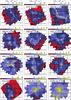 |
Fig. B.1 Column density maps of the fields (see Fig. 6 and Sect. 3.1.2 for details). |
| In the text | |
|
Fig. B.1 continued. |
| In the text | |
|
Fig. B.1 continued. |
| In the text | |
|
Fig. B.1 continued. |
| In the text | |
|
Fig. B.1 continued. |
| In the text | |
|
Fig. C.1 Cross sections of the surface brightness data along the lines indicated in Figs. 4, 5 and in the figures of Appendix A. The lines show the 250 μm SPIRE data (thick black line), AKARI 140 μm and 90 μm data (solid and dashed blue lines), and, when available, the WISE 22 μm data (dotted line). The average surface brightness in the reference region has been subtracted from the plotted values. The red thick line is the colour temperature. The data have been convolved to the resolution of one arc minute. The 90 μm data have been scaled by a factor 20 and the 22 μm data by a factor of 600. When a different scaling has been used, the wavelength and the multiplicative scaling factor are given in the frame (λ:factor). |
| In the text | |
|
Fig. C.1 continued. |
| In the text | |
|
Fig. C.1 continued. |
| In the text | |
|
Fig. C.1 continued. |
| In the text | |
|
Fig. C.1 continued. |
| In the text | |
|
Fig. D.1 Properties of a filament in the field G1.94+6.07. The frame a shows the column density map. The white line shows the filament that was originally traced by eye and the yellow line follows the ridge that is formed by the peaks of the column density profiles in the perpendicular direction. The black filled circle indicates the start of the examined filament section. The tick marks are drawn at 5 arcmin intervals. The frame b shows the average column density profile of the filament (black line), as well as the Plummer profile (the red dashed line on top of the black line) that was fitted together with a linear baseline (the blue dashed line) over the range −0.4 pc to +0.4 pc. The yellow lines show individual column density profiles for 20% of the cuts with the highest column densities (values normalized to a peak value of one, the right hand scale). The frame c shows the FWHM values (the black circles) and the parameter Rflat of the Plummer fit (the red crosses), and the column density along the ridge of the filament (the solid line and the right hand scale) as a function of the distance along the filament. |
| In the text | |
|
Fig. D.2 The filament selected from the field G82.65-2.00. |
| In the text | |
|
Fig. D.3 The filament selected from the field G89.65-7.02. |
| In the text | |
|
Fig. D.4 The filament selected from the field G94.15+6.50. |
| In the text | |
|
Fig. D.5 The filament selected from the field G98.00+8.75. |
| In the text | |
|
Fig. D.6 The filament selected from the field G105.57+10.39. |
| In the text | |
|
Fig. D.7 The filament selected from the field G126.63+24.55. |
| In the text | |
|
Fig. D.8 The filament selected from the field G149.67+3.56. |
| In the text | |
|
Fig. D.9 The filament selected from the field G157.08-8.68. |
| In the text | |
|
Fig. D.10 The filament selected from the field G157.92-2.28. |
| In the text | |
|
Fig. D.11 The filament selected from the field G159.34+11.21. |
| In the text | |
|
Fig. D.12 The filament selected from the field G161.55-9.30. |
| In the text | |
|
Fig. D.13 The filament selected from the field G164.71-5.64. |
| In the text | |
|
Fig. D.14 The filament selected from the field G167.20-8.69. |
| In the text | |
|
Fig. D.15 The filament selected from the field G176.27-2.09. |
| In the text | |
|
Fig. D.16 The filament selected from the field G181.84-18.46. |
| In the text | |
|
Fig. D.17 The filament selected from the field G198.58-9.10. |
| In the text | |
|
Fig. D.18 The filament selected from the field G203.42-8.29. |
| In the text | |
|
Fig. D.19 The filament selected from the field G205.06-6.04. |
| In the text | |
|
Fig. D.20 The filament selected from the field G210.90-36.55. |
| In the text | |
|
Fig. D.21 The filament selected from the field G212.07-15.21. |
| In the text | |
|
Fig. D.22 The filament selected from the field G215.44-16.38. |
| In the text | |
|
Fig. D.23 The filament selected from the field G276.78+1.75. |
| In the text | |
|
Fig. D.24 The filament selected from the field G298.31-13.05. |
| In the text | |
|
Fig. E.1 Spectral energy distributions corresponding to the apertures marked in the figures of Appendix A. The plots include 22 μm WISE data, AKARI data at 65 μm, 90 μm, 140 μm, and 160 μm, and the three SPIRE channels at 250 μm, 350 μm, and 500 μm. In most fields two aperture positions were chosen and the data for the second one are shown in red. The background subtraction was done using the reference areas marked in the figures of Appendix A (solid symbols) or by using a local annulus (open symbols). The colour temperatures from the modified blackbody fits with β = 2 are listed in the frames. |
| In the text | |
|
Fig. E.1 continued. |
| In the text | |
|
Fig. E.1 continued. |
| In the text | |
|
Fig. E.1 continued. |
| In the text | |
|
Fig. E.1 continued. |
| In the text | |
Current usage metrics show cumulative count of Article Views (full-text article views including HTML views, PDF and ePub downloads, according to the available data) and Abstracts Views on Vision4Press platform.
Data correspond to usage on the plateform after 2015. The current usage metrics is available 48-96 hours after online publication and is updated daily on week days.
Initial download of the metrics may take a while.