Galactic cold cores - III. General cloud properties

Free Access

Issue		A&A Volume 541, May 2012


Article Number		A12
Number of page(s)		89
Section		Interstellar and circumstellar matter
DOI		https://doi.org/10.1051/0004-6361/201118640
Published online		19 April 2012

Online material

Appendix A: Maps of observed and derived quantities

Figures A.1–A.69 show maps of observed and derived quantities for the fields other than the one already shown in Figs. 4, 5. Included in the figures are the colour temperature map derived from SPIRE data (frame a, 40″ resolution), the 250 μm SPIRE surface brightness map (frame b, 18″ resolution), the AKARI wide filter maps at 140 μm and 90 μm (frames c and e; convolved to a resolution of one arc minute), the visual extinction A_V derived from 2MASS catalogue stars (frame d; resolution of 2′), and the WISE 22 μm intensity (frame f; 12″ resolution). In the cases where public WISE data were not yet available, frame f shows the 25 μm IRAS map (resolution of 4.5′). The respective beam sizes are indicated in the lower right hand corner of each frame. The black circles indicate the positions of clumps selected for further examination in Sect. 3.2.1 and the white circles indicates a reference region used for background subtraction in the SED plots in Sect. 3.2.1. In frame a, the arrow indicates the position of the stripe plotted in Appendix C.

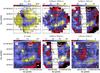Fig. A.1

Data on the field G1.94+6.07. Shown are the colour temperature map derived from SPIRE data (frame a, 40″ resolution), the 250 μm SPIRE surface brightness map (frame b, 18″ resolution), the AKARI wide filter maps at 140 μm and 90 μm (frames c and e), the visual extinction A_V derived from 2MASS catalog stars (frame d), and the WISE 22 μm intensity (frame f). In the subsequent figures, if public WISE data are not available, frame f shows the 25 μm IRAS map instead. The respective beam sizes are indicated in the lower right hand corner of each frame. The positions of selected clumps (black circles; see Sect. 3.2.1) and the reference regions used for background subtraction (white circle; see Sect. 3.2.1) are also shown.

Open with DEXTER

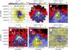	Fig. A.2 Data on the field G6.03+36.73.
Open with DEXTER

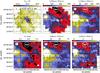	Fig. A.3 Data on the field G10.20+2.39.
Open with DEXTER

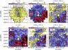	Fig. A.4 Data on the field G20.72+7.07.
Open with DEXTER

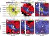	Fig. A.5 Data on the field G21.26+12.11.
Open with DEXTER

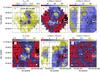	Fig. A.6 Data on the field G24.40+4.68.
Open with DEXTER

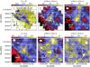	Fig. A.7 Data on the field G25.86+6.22.
Open with DEXTER

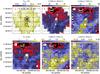	Fig. A.8 Data on the field G26.34+8.65.
Open with DEXTER

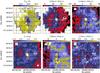	Fig. A.9 Data on the field G37.49+3.03.
Open with DEXTER

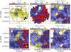	Fig. A.10 Data on the field G39.65+1.75.
Open with DEXTER

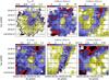	Fig. A.11 Data on the field G62.16-2.92.
Open with DEXTER

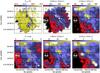	Fig. A.12 Data on the field G69.57-1.74.
Open with DEXTER

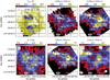	Fig. A.13 Data on the field G70.10-1.69.
Open with DEXTER

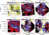	Fig. A.14 Data on the field G82.65-2.00.
Open with DEXTER

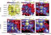	Fig. A.15 Data on the field G86.97-4.06.
Open with DEXTER

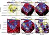	Fig. A.16 Data on the field G89.65-7.02.
Open with DEXTER

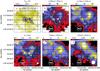	Fig. A.17 Data on the field G93.21+9.55.
Open with DEXTER

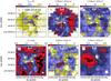	Fig. A.18 Data on the field G94.15+6.50.
Open with DEXTER

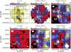	Fig. A.19 Data on the field G98.00+8.75.
Open with DEXTER

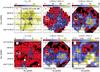	Fig. A.20 Data on the field G105.57+10.39.
Open with DEXTER

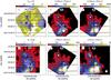	Fig. A.21 Data on the field G107.20+5.52 (PCC249).
Open with DEXTER

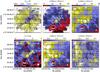	Fig. A.22 Data on the field G108.28+16.68.
Open with DEXTER

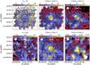	Fig. A.23 Data on the field G109.18-37.59.
Open with DEXTER

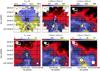	Fig. A.24 Data on the field G109.80+2.70 (PCC288).
Open with DEXTER

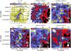	Fig. A.25 Data on the field G110.89-2.78.
Open with DEXTER

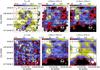	Fig. A.26 Data on the field G111.41-2.95.
Open with DEXTER

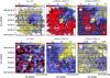	Fig. A.27 Data on the field G126.63+24.55.
Open with DEXTER

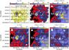	Fig. A.28 Data on the field G127.79+2.66.
Open with DEXTER

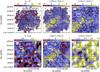	Fig. A.29 Data on the field G130.42-47.07.
Open with DEXTER

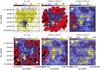	Fig. A.30 Data on the field G131.65+9.75.
Open with DEXTER

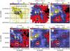	Fig. A.31 Data on the field G132.12+8.95.
Open with DEXTER

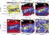	Fig. A.32 Data on the field G149.67+3.56.
Open with DEXTER

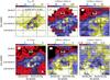	Fig. A.33 Data on the field G150.47+3.93.
Open with DEXTER

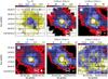	Fig. A.34 Data on the field G151.45+3.95.
Open with DEXTER

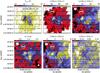	Fig. A.35 Data on the field G154.08+5.23.
Open with DEXTER

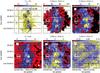	Fig. A.36 Data on the field G157.08-8.68.
Open with DEXTER

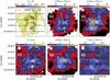	Fig. A.37 Data on the field G157.92-2.28.
Open with DEXTER

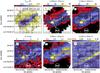	Fig. A.38 Data on the field G159.34+11.21.
Open with DEXTER

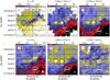	Fig. A.39 Data on the field G161.55-9.30.
Open with DEXTER

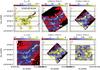	Fig. A.40 Data on the field G163.82-8.44.
Open with DEXTER

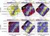	Fig. A.41 Data on the field G164.71-5.64.
Open with DEXTER

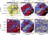	Fig. A.42 Data on the field G167.20-8.69.
Open with DEXTER

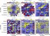	Fig. A.43 Data on the field G168.85-10.19.
Open with DEXTER

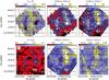	Fig. A.44 Data on the field G173.43-5.44.
Open with DEXTER

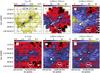	Fig. A.45 Data on the field G176.27-2.09.
Open with DEXTER

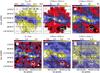	Fig. A.46 Data on the field G181.84-18.46.
Open with DEXTER

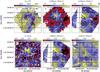	Fig. A.47 Data on the field G188.24-12.97.
Open with DEXTER

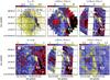	Fig. A.48 Data on the field G189.51-10.41.
Open with DEXTER

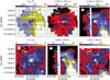	Fig. A.49 Data on the field G195.74-2.29.
Open with DEXTER

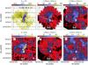	Fig. A.50 Data on the field G198.58-9.10.
Open with DEXTER

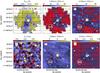	Fig. A.51 Data on the field G202.23-3.38.
Open with DEXTER

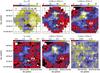	Fig. A.52 Data on the field G203.42-8.29.
Open with DEXTER

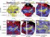	Fig. A.53 Data on the field G205.06-6.04.
Open with DEXTER

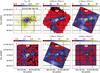	Fig. A.54 Data on the field G210.90-36.55.
Open with DEXTER

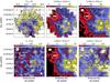	Fig. A.55 Data on the field G212.07-15.21.
Open with DEXTER

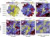	Fig. A.56 Data on the field G215.37-3.04.
Open with DEXTER

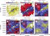	Fig. A.57 Data on the field G215.44-16.38.
Open with DEXTER

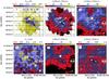	Fig. A.58 Data on the field G216.76-2.58.
Open with DEXTER

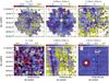	Fig. A.59 Data on the field G218.06+2.12.
Open with DEXTER

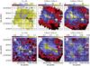	Fig. A.60 Data on the field G227.95-2.98.
Open with DEXTER

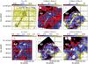	Fig. A.61 Data on the field G276.78+1.75.
Open with DEXTER

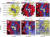	Fig. A.62 Data on the field G298.31-13.05.
Open with DEXTER

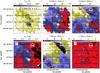	Fig. A.63 Data on the field G300.61-3.13.
Open with DEXTER

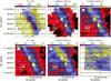	Fig. A.64 Data on the field G300.86-9.00 (PCC550).
Open with DEXTER

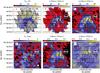	Fig. A.65 Data on the field G315.88-21.44.
Open with DEXTER

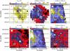	Fig. A.66 Data on the field G334.65+2.67.
Open with DEXTER

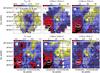	Fig. A.67 Data on the field G339.22-6.02.
Open with DEXTER

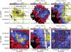	Fig. A.68 Data on the field G343.64-2.31.
Open with DEXTER

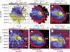	Fig. A.69 Data on the field G358.96+36.75.
Open with DEXTER

Appendix B: Column density maps

Figure B.1 shows the column density maps for all the fields excluding those already shown in Fig. 6.

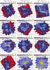	Fig. B.1 Column density maps of the fields (see Fig. 6 and Sect. 3.1.2 for details).
Open with DEXTER

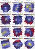	Fig. B.1 continued.
Open with DEXTER

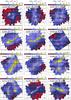	Fig. B.1 continued.
Open with DEXTER

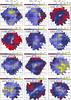	Fig. B.1 continued.
Open with DEXTER

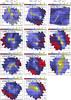	Fig. B.1 continued.
Open with DEXTER

Appendix C: One-dimensional cuts of the surface brightness data

Figure C.1 shows selected surface brightness values along the one-dimensional cuts marked in the frames a of Fig. 4 and Figs. A.1–A.69.

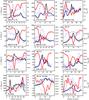Fig. C.1

Cross sections of the surface brightness data along the lines indicated in Figs. 4, 5 and in the figures of Appendix A. The lines show the 250 μm SPIRE data (thick black line), AKARI 140 μm and 90 μm data (solid and dashed blue lines), and, when available, the WISE 22 μm data (dotted line). The average surface brightness in the reference region has been subtracted from the plotted values. The red thick line is the colour temperature. The data have been convolved to the resolution of one arc minute. The 90 μm data have been scaled by a factor 20 and the 22 μm data by a factor of 600. When a different scaling has been used, the wavelength and the multiplicative scaling factor are given in the frame (λ:factor).

Open with DEXTER

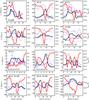	Fig. C.1 continued.
Open with DEXTER

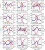	Fig. C.1 continued.
Open with DEXTER

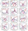	Fig. C.1 continued.
Open with DEXTER

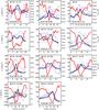	Fig. C.1 continued.
Open with DEXTER

Appendix D: Figures of the selected elongated cloud structures

The analysis of the filamentS in the fields G163.82-8.44 and G300.86-9.00 (PCC 550) were shown in Figs. 7, 8. The plots for the other fields listed in Table 3 are shown in Figs. D.1–D.24. These include only the fields with an existing distance estimate and where a clear filament or other distinct elongated structure could be discerned.

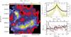Fig. D.1

Properties of a filament in the field G1.94+6.07. The frame a shows the column density map. The white line shows the filament that was originally traced by eye and the yellow line follows the ridge that is formed by the peaks of the column density profiles in the perpendicular direction. The black filled circle indicates the start of the examined filament section. The tick marks are drawn at 5 arcmin intervals. The frame b shows the average column density profile of the filament (black line), as well as the Plummer profile (the red dashed line on top of the black line) that was fitted together with a linear baseline (the blue dashed line) over the range −0.4 pc to +0.4 pc. The yellow lines show individual column density profiles for 20% of the cuts with the highest column densities (values normalized to a peak value of one, the right hand scale). The frame c shows the FWHM values (the black circles) and the parameter R_flat of the Plummer fit (the red crosses), and the column density along the ridge of the filament (the solid line and the right hand scale) as a function of the distance along the filament.

Open with DEXTER

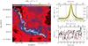	Fig. D.2 The filament selected from the field G82.65-2.00.
Open with DEXTER

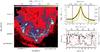	Fig. D.3 The filament selected from the field G89.65-7.02.
Open with DEXTER

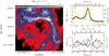	Fig. D.4 The filament selected from the field G94.15+6.50.
Open with DEXTER

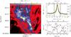	Fig. D.5 The filament selected from the field G98.00+8.75.
Open with DEXTER

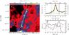	Fig. D.6 The filament selected from the field G105.57+10.39.
Open with DEXTER

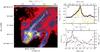	Fig. D.7 The filament selected from the field G126.63+24.55.
Open with DEXTER

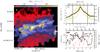	Fig. D.8 The filament selected from the field G149.67+3.56.
Open with DEXTER

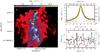	Fig. D.9 The filament selected from the field G157.08-8.68.
Open with DEXTER

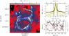	Fig. D.10 The filament selected from the field G157.92-2.28.
Open with DEXTER

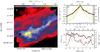	Fig. D.11 The filament selected from the field G159.34+11.21.
Open with DEXTER

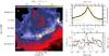	Fig. D.12 The filament selected from the field G161.55-9.30.
Open with DEXTER

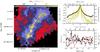	Fig. D.13 The filament selected from the field G164.71-5.64.
Open with DEXTER

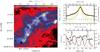	Fig. D.14 The filament selected from the field G167.20-8.69.
Open with DEXTER

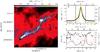	Fig. D.15 The filament selected from the field G176.27-2.09.
Open with DEXTER

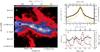	Fig. D.16 The filament selected from the field G181.84-18.46.
Open with DEXTER

	Fig. D.17 The filament selected from the field G198.58-9.10.
Open with DEXTER

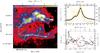	Fig. D.18 The filament selected from the field G203.42-8.29.
Open with DEXTER

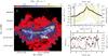	Fig. D.19 The filament selected from the field G205.06-6.04.
Open with DEXTER

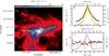	Fig. D.20 The filament selected from the field G210.90-36.55.
Open with DEXTER

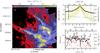	Fig. D.21 The filament selected from the field G212.07-15.21.
Open with DEXTER

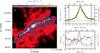	Fig. D.22 The filament selected from the field G215.44-16.38.
Open with DEXTER

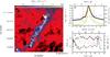	Fig. D.23 The filament selected from the field G276.78+1.75.
Open with DEXTER

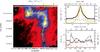	Fig. D.24 The filament selected from the field G298.31-13.05.
Open with DEXTER

Appendix E: Spectra of selected regions

The spectral energy distributions of selected regions were presented in Fig. 10. Similar figures for the remaining fields are shown in Fig. E.1.

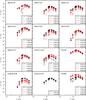Fig. E.1

Spectral energy distributions corresponding to the apertures marked in the figures of Appendix A. The plots include 22 μm WISE data, AKARI data at 65 μm, 90 μm, 140 μm, and 160 μm, and the three SPIRE channels at 250 μm, 350 μm, and 500 μm. In most fields two aperture positions were chosen and the data for the second one are shown in red. The background subtraction was done using the reference areas marked in the figures of Appendix A (solid symbols) or by using a local annulus (open symbols). The colour temperatures from the modified blackbody fits with β = 2 are listed in the frames.

Open with DEXTER

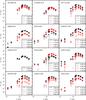	Fig. E.1 continued.
Open with DEXTER

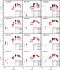	Fig. E.1 continued.
Open with DEXTER

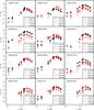	Fig. E.1 continued.
Open with DEXTER

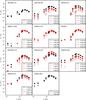	Fig. E.1 continued.
Open with DEXTER

© ESO, 2012

Current usage metrics show cumulative count of Article Views (full-text article views including HTML views, PDF and ePub downloads, according to the available data) and Abstracts Views on Vision4Press platform.

Data correspond to usage on the plateform after 2015. The current usage metrics is available 48-96 hours after online publication and is updated daily on week days.

Initial download of the metrics may take a while.