| Issue |
A&A
Volume 688, August 2024
|
|
|---|---|---|
| Article Number | A171 | |
| Number of page(s) | 24 | |
| Section | Extragalactic astronomy | |
| DOI | https://doi.org/10.1051/0004-6361/202349027 | |
| Published online | 20 August 2024 | |
Molecular cloud matching in CO and dust in M33
I. High-resolution hydrogen column density maps from Herschel
1
I. Physikalisches Institut, Universität zu Köln, Zülpicher Straße 77, 50937 Köln, Germany
2
School of Astronomy, Institute for Research in Fundamental Sciences (IPM), PO Box 19395-5531 Tehran, Iran
3
Max-Planck-Institut für Astronomie, Königstuhl 17, 69117 Heidelberg, Germany
4
Argelander-Institut für Astronomie, Universität Bonn, Auf dem Hügel 71, 53121 Bonn, Germany
Received:
19
December
2023
Accepted:
22
April
2024
This study is aimed to contribute to a more comprehensive understanding of the molecular hydrogen distribution in the galaxy M33 by introducing novel methods for generating high angular resolution (18.2″, equivalent to 75 pc for a distance of 847 kpc) column density maps of molecular hydrogen (NH2). M33 is a local group galaxy that has been observed with Herschel in the far-infrared (FIR) wavelength range from 70 to 500 μm. Previous studies have presented total hydrogen column density maps (NH), using these FIR data (partly combined with mid-IR maps), employing various methods. We first performed a spectral energy distribution (SED) fit to the 160, 250, 350, and 500 μm continuum data obtain NH, using a technique similar to one previously reported in the literature. We also use a second method which involves translating only the 250 μm map into a NH map at the same angular resolution of 18.2″. An NH2 map via each method is then obtained by subtracting the H I component. Distinguishing our study from previous ones, we adopt a more versatile approach by considering a variable emissivity index, β, and dust absorption coefficient, κ0. This choice enables us to construct a κ0 map, thereby enhancing the depth and accuracy of our investigation of the hydrogen column density. We address the inherent biases and challenges within both methods (which give similar results) and compare them with existing maps available in the literature. Moreover, we calculate a map of the carbon monoxide CO(1 − 0)-to-molecular hydrogen (H2) conversion factor (XCO factor), which shows a strong dispersion around an average value of 1.8 × 1020 cm−2/(K km s−1) throughout the disk. We obtain column density probability distribution functions (N-PDFs) from the NH, NH2, and NH I maps and discuss their shape, consisting of several log-normal and power-law tail components.
Key words: methods: analytical / dust / extinction / ISM: general / ISM: structure / galaxies: ISM / Local Group
© The Authors 2024
 Open Access article, published by EDP Sciences, under the terms of the Creative Commons Attribution License (https://creativecommons.org/licenses/by/4.0), which permits unrestricted use, distribution, and reproduction in any medium, provided the original work is properly cited.
This article is published in open access under the Subscribe to Open model. Subscribe to A&A to support open access publication.
1. Introduction
Column density maps obtained from dust observations in the mid and far-infrared (MIR-FIR) to submillimetre wavelengths are valuable indicators of a galaxy’s total hydrogen content. Spectral energy distribution (SED) fits to the flux maps acquired through Herschel provide a commonly used measure of the total hydrogen column density, expressed as  . This method of analysis assumes the absence of an ionised gas contribution. Subtracting an H I column density map from the map of NH allows us to construct a map of the total molecular gas, as done in Braine et al. (2010b) for the Triangulum galaxy M33 (cf. see their Fig. 4). However, high angular resolution dust maps are limited in availability, making comprehensive maps exceedingly valuable. The HerM33es Key Project provides the required data sets for M33, namely, full continuum mapping using Herschel (Kramer et al. 2010). It also delivers a 12CO(2 − 1) map via an IRAM 30m Large Program (Druard et al. 2014).
M33 is an Sc-type spiral galaxy at a distance of 847 kpc (Karachentsev et al. 2004). Its proximity and inclination angle of ∼56° (Regan & Vogel 1994) allow for resolving individual giant molecular clouds (GMCs). 18.2″ correspond to ∼75 pc at the distance cited, which is the size of large cloud complexes in the Milky Way (Nguyen-Luong et al. 2016). In optical and infrared images, M33 displays a spiral structure, containing numerous distinct, massive star-forming regions alongside a diffuse extended component. The metallicity of M33 has been determined using various methods, mostly relying on measurements of neon and oxygen abundances in H II regions (Willner & Nelson-Patel 2002; Crockett et al. 2006; Magrini et al. 2009). These studies show a large scatter in absolute values of the metallicity (ranging from values comparable to the Milky Way to lower ones), but consistently suggest that it varies with galactocentric radius. The largest sample of H II regions in M33 is presented by Rosolowsky et al. (2008), Relaño et al. (2016). They also find that the metallicity is a function of galactocentric radius. The overall average metallicity they derive is approximately half of the Milky Way value and is frequently cited in the literature. Despite its relatively modest mass, which is only about 10% of that of the Milky Way, M33 serves as a crucial link between objects with lower metallicity and more irregular structures such as the Large Magellanic Cloud, as well as more evolved spiral galaxies such as the Milky Way.
Several dust column density maps (and from that NH maps) have been derived for M33 using mostly SED fits to FIR data from Herschel (Braine et al. 2010b; Tabatabaei et al. 2014; Relaño et al. 2018; Clark et al. 2021, 2023). However, each map has been created with different assumptions on the absorption coefficient κ0, dust, the emissivity index β and the dust-to-gas ratio (DGR). For example, Braine et al. (2010b) derived a column density map with a variable absorption coefficient, κ0, in the dust opacity law, but with a fixed emissivity index, β. Tabatabaei et al. (2014) obtained a map of β and dust surface densities that were shown for both the cold and warm gas components. Other studies such as Clark et al. (2021) employed a fixed DGR and a broken emissivity law with a modified blackbody.
The approach presented here is novel because we use a variable dust emissivity index, β, and a spatial map of the absorption coefficient, κ0, DGR, in which the DGR is intrinsically included. For that purpose, we employ the map of β indices given by Tabatabaei et al. (2014) as well as their temperature map of the cold dust component, obtained from a two-component model with a constant κ0, dust for the dust.
It is one objective of this paper to confront the different methods used to obtain hydrogen column density maps with each other and discuss their individual biases. With the β and κ0, DGR maps, we then perform an SED fit to the Herschel data (method I) and convert the 250 μm Herschel map (method II) to obtain the total hydrogen column density map. From these maps, we then subtract the H I component to derive the H2 column density maps.
Another way of obtaining a map of molecular hydrogen is to use observations of CO. The H2 molecule is difficult to observe directly, primarily due to its low moment of inertia and consequently high rotational energy, which requires high temperatures to excite rotational transitions, and its lack of a dipole moment. As a surrogate for H2, the second most abundant molecule, CO, is commonly used to trace H2. The low-J rotational transitions of CO serve as effective tracers for the cold regions of molecular clouds. This is due to their low excitation temperatures (up to a few tens of Kelvin) and low critical densities (typically below 103 cm−3) for collisional excitation. Consequently, the mass of molecular gas in interstellar clouds is typically determined by employing a CO-to-H2 conversion factor, denoted as XCO, which scales the observed CO line intensities ICO to molecular hydrogen column densities NH2 (Bloemen et al. 1986; Israel 1997; Bolatto et al. 2013; Borchert et al. 2022). The relationship is expressed as: NH2 = XCO × ICO. For the Milky Way, the so-called ‘XCO factor’ is approximately 2 × 1020 cm−2/(K km s−1), showing an increase from the centre to the outer disk (Sodroski et al. 1995; Bolatto et al. 2013; Veltchev et al. 2018). While studying galaxies in the local universe and at higher redshifts, CO observations are commonly employed to investigate individual cloud masses (Leroy et al. 2011; Bigiel et al. 2011; Cormier et al. 2014; Tacconi et al. 2018). However, the XCO factor exhibits significant variations due to differing metallicities. In environments with low metallicity, the XCO factor is expected to be higher than the standard value, which is attributed to a lower GDR (Leroy et al. 2013). However, this is challenged by a recent study of Ramambason et al. (2023), Chiang et al. (2024) that shows a very large variation of the XCO factor in nearby dwarf galaxies and by den Brok et al. (2023) who showed a variation of the XCO factor across the M101 galaxy.
The influence of far-ultraviolet (FUV) photons from massive stars also has an impact on the abundance of CO and the other carbon derivatives. In regions with lower metallicity, the FUV photons reach deeper into molecular clouds. These photons photodissociate CO and ionise carbon, leading to the creation of C+. Consequently, a larger C+-emitting envelope surrounds a more compact CO core in such environments. Simultaneously, H2 photodissociates upon absorbing Lyman-Werner band photons. In denser regions, H2 can become optically thick, thereby self-shielding from photodissociation. As a consequence, a substantial reservoir of molecular hydrogen exists beyond the CO-emitting region. This region is often referred to as CO-dark H2 gas (Röllig et al. 2006; Wolfire et al. 2010; Pineda et al. 2013, 2014). Models (Clark et al. 2019b) predict that ionised and neutral carbon can serve as mass tracers for this CO-dark molecular gas (for a more in-depth discussion, we refer to Madden et al. 2020).
M33 has been extensively studied in CO and other molecular lines with the IRAM 30m telescope and the Plateau de Bure Interferometre (see Gratier et al. 2010 for a compilation of CO surveys with other telescopes) and with Herschel in the FIR to submm continuum. These studies focus on the dust properties (Boquien et al. 2011; Xilouris et al. 2012; Tabatabaei et al. 2014; Relaño et al. 2016, 2018), the star-formation rate (Gardan et al. 2007; Verley et al. 2010a; Boquien et al. 2010, 2015), the XCO factor (Braine et al. 2010a,b), individual sources (Braine et al. 2012b,a; Gratier et al. 2012), the dense gas properties (Buchbender et al. 2013), the CO(2 − 1) mapping (Gratier et al. 2010; Druard et al. 2014), the gas cooling via FIR lines (Kramer et al. 2020), the properties of H II regions (Relaño et al. 2013), and on the 250 μm dust sources (Verley et al. 2010b).
In this paper, we produce high angular resolution (18.2″) NH and NH2 maps with two methods. We start with a description of the available data sets (Sect. 2) and continue with an outline of the methods (Sect. 3), including a discussion of the assumptions and shortcomings of the procedures. Section 4 shows the column density probability distribution functions (N-PDFs), presents and compares the dust-derived H2 column density maps and the one obtained from CO and shows a map of the XCO factor. In Sect. 5, we put our column density maps into context with others available in the literature. Section 6 summarises the paper.
2. Data
2.1. Herschel data
We utilise the FIR Herschel imaging data between 160 and 500 μm, which were observed in the framework of the Herschel Key Project HerM33es1 (Kramer et al. 2010; Boquien et al. 2010, 2011; Xilouris et al. 2012; Tabatabaei et al. 2014). The shorter wavelength maps at 70 and 100 μm are omitted because we focus on the cold gas, characterised by dust temperatures typically below 20 − 30 K, which exhibits an SED peak around 250 μm. We thus use the PACS flux map at 160 μm, featuring an angular resolution of approximately 11″ and the SPIRE flux maps at 250 μm, 350 μm, and 500 μm, with angular resolutions of approximately 18″, 25″, and 36″, respectively. For the PACS maps, we employ the JScanam data products, obtained using the Scanamorphos algorithm (Roussel 2013), which have previously been used by HerM33es for earlier versions of the PACS maps. The data used for the analysis are from level 2.5 archives, processed with a calibration tree update beyond the calibration used for the original HerM33es maps. For SPIRE, we use data directly from the Herschel science archive that uses HIPE v14 photometric calibrations. The data have been reduced with the relative gains of the SPIRE bolometers optimised to detect extended emission, using the beam area values provided in HIPE v15. As with all SPIRE final data products, all maps have been produced using the SPIRE de-striper to eliminate artefacts arising from instrumental drift. All flux maps used in this paper are shown in their native resolution in Fig. A.1. For a detailed overview of the Herschel data products, we refer to the publications of the HerM33es team and Clark et al. (2021).
2.2. VLA H I integrated intensity data
In order to extract only the H2 gas from the total hydrogen column density map we derive from the Herschel data, it is required to remove the atomic hydrogen contribution. For that, we employed an H I map observed with the VLA at a resolution of 12″ (Gratier et al. 2010). This H I map recovers ∼90% of the flux detected by Putman et al. (2009) using the Arecibo Observatory.
We smoothed the VLA map to an angular resolution of 18.2″ using a Gaussian kernel, re-gridded the map and then transformed the integrated intensity to column density (Rohlfs & Wilson 1996) assuming warm, optically thin emission with:
in which Tmb is the main beam brightness temperature in (K) and dv the velocity range in (km s−1). This H I column density map is shown in the left panel of Fig. 1 with CO contour lines overlaid. Regions of peak emission are associated with the GMCs in the spiral arms, but there is also significant, more diffuse emission in the region between the arms. The mean noise of the map is ∼2 × 1020 cm−2.
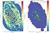 |
Fig. 1. NH I and CO line-integrated intensity map. Left: H I column density map determined from VLA H I observations (Gratier et al. 2010). Right: IRAM 30 m CO(2 − 1) line integrated intensity map of M33 (Druard et al. 2014). The lines in the colour bar mark the 3σ and 6σ values of CO emission. Both maps are smoothed to a resolution of 18.2″ and re-gridded to a pixel size of 6″. CO contours at 3 and 6σ are overlaid on both maps. |
2.3. IRAM 30 m telescope 12CO(2 − 1) data
M33 has been observed in the 12CO(2 − 1) line2 with the HERA multibeam dual-polarisation receiver in the on-the-fly mapping mode within the https://iram-institute.org/science-portal/proposals/lp/completed/lp006-the-complete-co2-1-map-of-m33/ “The complete CO(2 − 1) map of M33” (see Gratier et al. 2010; Druard et al. 2014). We obtained the CO data cube and the line integrated map from the https://www.iram.fr/ILPA/LP006/. This data cube has an angular resolution of 12″ and a spectral resolution of 2.6 km s−1, with a mean rms noise of 20.33 mK per velocity channel (Druard et al. 2014). In order to compare with the dust map, we smoothed the line integrated map to 18.2″ resolution using a Gaussian kernel. We here only use the line integrated CO intensity map for which we determined an rms noise of 0.35 K km s−1, corresponding to 3σ = 1.046 K km s−1, from the smoothed 18.2″ map. The temperature scale of the archive data is in antenna temperatures and has been converted into main beam brightness temperatures using a forward efficiency of Feff = 0.92 and a beam efficiency of Beff = 0.56 (Druard et al. 2014). The final CO map is shown in the right panel of Fig. 1.
3. Hydrogen column density maps from Herschel flux maps
This section first gives a derivation of the basic equations to obtain the total hydrogen column density, NH, which is essential for both methods discussed in the following, as well as the properties of the dust emissivity index and absorption coefficient. The subsequent subsections describe the two methods deriving high-resolution (high-res) column density maps at 18.2″ from the Herschel flux maps and how the H2 maps are produced3.
3.1. Derivation of NH
The flux density of the continuum emission, Fν, is related to the Planck law, Bν(Td), and optical depth, τν, via:
![$$ \begin{aligned} F_\nu = B_\nu (T_{\rm d})[1-e^{-\tau _\nu }]\,\Omega ~, \end{aligned} $$](/articles/aa/full_html/2024/08/aa49027-23/aa49027-23-eq3.gif)
with the Planck law
Herewith, ν represents the frequency, Td denotes the dust temperature (free or fixed; see below), and Ω represents the solid angle of the source. For a low optical depth, which can generally be assumed for dust, τν ≪ 1, we can approximate the above expression by
Since the specific intensity is given by Iν = Fν/Ω and
where Md is the dust mass, κd(ν) is the dust opacity or the extinction cross-section per dust mass (the subscript d stands for the dust), and D2 is the distance squared to M33, the specific intensity, Iν, is then:
Introducing the dust-to-gas ratio (DGR), we can rewrite the last equation as
Defining κg(ν):=κd(ν)⋅DGR, where the subscript g stands for gas, as well as Mgas := Md/DGR leads to
Here, κg(ν) is the dust opacity per unit mass (total mass of gas and dust). The number of gas particles, Ng, multiplied by the mean molecular weight, μm, and the hydrogen mass, mH, yields the gas mass, Mgas, the column density, NH, can be related to the number of particles by NH = Ng/(D2Ω), so that the specific intensity can eventually be written as:

Assuming a power-law frequency-dependent κg(ν) (Juvela et al. 2015b), we can write the above equation as:

where a dust opacity law similar to Krügel & Siebenmorgen (1994) has been used with

Here, κ0, DGR is the absorption coefficient in units of (cm2/g) with the DGR inherently included, which will be described in Sect. 3.2, and β is the emissivity index. We will denote κ0, DGR simply as κ0 from now on. The hydrogen column density NH is calculated from the surface density Σ = μm mH NH, with a mean molecular weight of μm = 1.36, and  . Re-arranging for the column density, NH, the above expression finally gives
The values of the parameters in the dust opacity law, κ0 and β, are crucial but their spatial variation is difficult to determine correctly. We devote Sect. 3.2 to a more detailed discussion. Note that the DGR is contained within κ0 in this notation.
We note that other studies often express κ0(λ/250 μm)−βμm mH = σH as the cross-section per H-atom, denoted as σH, which writes Eq. (12) equivalently to
3.2. The dust absorption coefficient, κ0, and emissivity index, β
A crucial point for SED fitting (described in Sect. 3.4) and the calculation of the column density is the choice of the dust absorption coefficient, κ0, and the dust emissivity index, β. The resolution of 18.2″ (equivalent to 75 pc) of our final hydrogen column density maps samples a mixture of dust and gas properties. The derived values of parameters such as β, κ0, or Td thus are intensity-weighted averages over the equivalent resolved beam area along the lines of sight. Different physical processes such as grain-grain collisions, condensation of molecules onto grains or shattering can affect the grain properties and, as such, the value of the emissivity index. The grain properties will vary within each beam, and the beam-averaged properties will also vary with the galactic environment, including factors such as star formation efficiency, metallicity, turbulence, and so on. Thus, the value of β is most likely not constant over a full galaxy, but rather depends on grain size, structure, distribution and chemical composition. A detailed discussion of the fundamentals is provided by Ossenkopf & Henning (1994). Observational constraints for Milky Way clumps are summarised by Juvela et al. (2015a,b). For particles small compared to the wavelength and non-changing optical constants, β would take the value of 1 from absorption in the Rayleigh limit (Krügel 2003). However, for any real material, this must break down at long wavelengths due to the integrability of the Kramers-Kronig relation for the optical constants. Ossenkopf & Henning (1994) showed that this leads to β = 2 for the bulk absorption in the millimetre regime and beyond, but shallower spectra with β = 1…2 were discussed for large coagulated grains in the wavelength range covered by Herschel. The range for β derived from observations lies between 1 and 2.5 (Chapin et al. 2011; Casey et al. 2011; Boselli et al. 2012). Boselli et al. (2012) found that β ≲ 1.5 provides a better fit for metal-poor, low surface brightness galaxies.
For M33, dust properties have been extensively studied (Boquien et al. 2011; Xilouris et al. 2012; Tabatabaei et al. 2014; Relaño et al. 2016, 2018). While Xilouris et al. (2012) assumed β = 1.5 for M33, Tabatabaei et al. (2014) derived a variable emissivity index for the cold dust component, which decreases along the galactocentric radius from β = 2 in the centre to β = 1.3 in the outer disk. This might reflect the complexity of the grain properties in more detail. Tabatabaei et al. (2014) applied a two-component modified blackbody fit to the SED using Spitzer and Herschel data ranging from 70 to 500 μm. The two-component model was solved for the dust temperature, β parameter and dust surface density.
With the emissivity index (Fig. B.2) and dust temperature map (Fig. B.3) from Tabatabaei et al. (2014) which we use here, the corresponding κ0 in the dust opacity law (Eq. (10)) will also vary pixel-by-pixel. The dust emission cross-section per H-atom, σH, can be related to the optical depth, τν, and total column density by (see Sect. 3.1, Eq. (13)):

where I250 μm is the specific intensity of the SPIRE 250 μm map and σH is given in Eq. (13).
Considering only regions with no or low CO emission allows us to avoid any assumptions on the CO-to-H2 conversion factor XCO. We therefore exclude regions above the 2σ level of the CO emission for the calculation of κ0 pixel-by-pixel, suggesting that the total hydrogen column density NH is dominated by the atomic hydrogen column density NH I. Using the relation κ0(λ/250 μm)−β μm mH = σH, Eq. (14) can then be re-arranged as follows:
which simplifies to
With this approach, we get some cavities in the κ0 map, where the CO emission exceeds its 2σ level (Fig. B.1). To fill these void regions, the machine learning interpolation technique KNNImputer from the scikit-learn Python package is employed (Pedregosa et al. 2011), as explained in Appendix B. The resulting κ0 map, which incorporates the interpolated values, is displayed in Fig. 2.
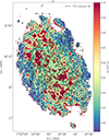 |
Fig. 2. κ0 map obtained as described in Sect. 3.2. Note that the DGR is included in the notation of κ0. CO contours at the 2σ level are overlaid on the map. |
At the edges of the galaxy, the κ0 values fall below 0.02 cm2 g−1, while in some regions around the two main spiral arms, very high values are reached (red in the colour scale of Fig. 2) due to low H I column densities. From these regions, some interpolated values of κ0 within the cavities in Fig. B.1 yield excessively high values in the molecular phase, resulting in negligible H2 column density in a few areas, such as the southern central part of M33. This occurs where the H I column density rapidly decreases, causing an exceptionally high value of κ0 (see Eq. (15)). This sharp transition in H I column density corresponds to a fast drop to the noise level of H I column density. Hence, our interpolation assigns very high values of κ0 to areas where the CO emission exceeds the 2σ level. This is due to our assumption of a non-changing κ0 and a lack of additional information on how κ0 should behave.
However, since we know that H2 must exist in these regions, we conclude that these κ0 values are too high. Testing with different values of κ0 manually reveals that a range of approximately 0.03 to 0.04 cm2 g−1 provides a lower limit for the H2 column density. To set the excessively high values of κ0 in a few regions to lower values, we calculate the median of the interpolated values after a first interpolation with KNNImputer. The median is ∼0.04 cm2 g−1 and is, hence, consistent with the lower limit for the H2 column density as determined above. The median gives a robust estimate of the interpolated κ0 values within the molecular phase, while the mean value is too sensitive to outliers (the excessively high values of κ0). Subsequently, where the edges of the cavities (at the CO 2σ emission) exceed this median of 0.04 cm2 g−1, we set κ0 = 0.04 cm2 g−1 for those pixels. The interpolated values from the first interpolation are then discarded and re-interpolated with these updated κ0 values at the edges of the cavities at the CO 2σ level. So, only those pixels at the edges of the cavities (at the CO 2σ level) are updated to the median value, where κ0 was higher than the median after the first interpolation. And then a second interpolation has been applied with these updated pixels.
This approach results in a more uniformly distributed κ0 within the molecular phase (or where CO exceeds the 2σ level), especially in the central part of the disk, aligning with our assumption of a constant κ0, as no further information on the behaviour of κ0 is available. One might argue for the adoption of a constant κ0 across the entire interpolated region, since we ‘update’ the values to the median. However, such an approach would lead to the loss of information in regions that fall below the median, as exactly these values contribute to the calculation of the median. Furthermore, since we lack any information on a lower limit for κ0, we have no additional justification for a universal update of κ0 throughout the region.
Previous studies often suffered from assumptions on the XCO factor, a fixed dust-absorption coefficient or from utilising a constant DGR. Our map intrinsically captures the overall trends on galactic scales, such as potential variations in the DGR or dependencies on the galactocentric radius. This is achieved by providing all relevant information on a pixel-by-pixel basis, thereby rendering the computation of κ0 for each pixel. As a result, the determination of the XCO factor remains unaffected by assumptions, allowing its evaluation while accounting for variations across the galactocentric radius. We note that the success of the interpolation technique relies on the assumption that the dust properties do not change significantly between the atomic and molecular phases. Further investigations are needed to confirm its applicability in specific cases.
With the method described above, we generate new high-resolution column density maps of M33, specifically focusing on the cold gas. However, accurately determining the final uncertainty of the map is challenging due to the involvement of multiple factors of uncertainty. Sources of uncertainty are introduced by the provided emissivity index map generated as discussed in Tabatabaei et al. (2014) and the calculated κ0 map determined from the emissivity index and the VLA H I map. A fixed κ0 = 0.038 cm2 g−1 determined as the mean value above the 2σ CO regions and increased by 20% alters the mean column density by a factor of less than ∼2 and ∼2.5, respectively, whereas increasing β by 20% does not change the mean by more than a factor of ∼0.8. Thus, we consider our generated column density map to be robust.
For any future reference, we will adopt the following terminology. With ‘inter-main spiral regions’, we refer to the area roughly inside the white dashed ellipses with a galactocentric distance of roughly 4 kpc in Fig. 3, excluding the two main spiral arms defined by the 3σ CO contours and the centre. Using the terms ‘outer region’ or ‘outskirts’ of M33, we specifically indicate the region roughly outside of those ellipses. We note that the white dashed ellipses are used solely to illustrate our terms and do not represent any physical means.
 |
Fig. 3. Total hydrogen column density maps obtained via methods I and II. Left: high resolution NH total gas column density map obtained from the Herschel maps of M33 at 18.2″ angular resolution using the β map from Tabatabaei et al. (2014) with method I. Right: total gas column density map NH obtained from the Herschel SPIRE 250 μm map of M33 with method II at the same spatial resolution of 18.2″, indicated by the circle in the lower left corner. CO contours (as of Fig. 1) are overlaid in both maps. The white dashed ellipses mark roughly the regions we refer to as ‘inter-main spiral’ region or “outskirts”. |
3.3. Preparation of the maps
Before running the code implemented to generate the high-resolution map, we applied a mask to the uneven edges of the original Herschel maps, which exhibit higher noise due to the scanning pattern of the telescope. The data obtained from the archive are absolutely calibrated, incorporating the necessary Planck-offset corrections for the SPIRE observations. They encompass emissions originating from the Milky Way. Consequently, we derived the average contribution from Galactic emissions in regions beyond the galaxy and subsequently subtracted the values thus determined from the maps (refer to Table A.1 in Appendix A for an overview of the background root-mean-square (rms) values). This procedure aligns with the methodology employed by the HerM33es consortium (Xilouris et al. 2012). The intensity units for all maps have been converted to MJy sr−1. Subsequently, we reproject and re-grid all maps to the central coordinates and grid pattern of 6″ of the SPIRE 250 μm map. The ensuing algorithm, outlined below, has then been applied to these reprocessed maps.
3.4. Method I: Dust column density map from SED fits to Herschel maps
This method requires several steps, which are described in the following sub-subsections.
3.4.1. Spatial decomposition
The conventional approach employed to generate column density maps from Herschel observations, primarily applied to Galactic data, involves fitting the dust temperature, Td, as well as β and the surface density, Σ, via a one-component greybody function (modified Planck function) pixel-by-pixel to the SED derived from the flux densities within the wavelength range of 160 to 500 μm. To allow for this, all flux maps are subject to smoothing, aligning them with the 500 μm map’s resolution of 36″, which serves as the lowest common resolution for the fitting process. Consequently, the resultant map adopts this resolution (e.g. André et al. 2010). An alternative technique for obtaining a higher angular resolution column density map at 18.2″, introduced by Palmeirim et al. (2013), is based on a multi-scale decomposition of the flux maps and has not yet been employed for extragalactic observations.
Imaging maps can be considered a superposition of emissions at many different spatial scales (e.g., Starck et al. 2004). For this reason, attempts have been made to describe the interstellar medium (ISM) as a two-component system, consisting of a more diffuse self-similar fractal component and a coherent, filamentary component (Robitaille et al. 2019), or as a multi-fractal system (Elia et al. 2018; Yahia et al. 2021). Methods to separate these structures are often based on wavelet, ridgelet and curvelet transforms. To create a high-resolution column density map, one must reverse this approach and construct a map from higher resolution sub-maps that still contain individual spatial scales, involving SED fits at different wavelengths. In the following, we outline the method presented in Appendix A of Palmeirim et al. (2013).
The high angular resolution (high-res from now on) map of the gas surface density distribution Σhigh at 18.2″ is given by:

where Σ500, Σ350, and Σ250 are the gas surface density distributions4 at the angular resolution of their corresponding Herschel bands, i.e. 36.3″, 24.9″, and 18.2″, respectively, and Gλc_λo are the Gaussian kernels of width  for the convolution, commonly denoted as *. The beam at the required resolution is specified by θc and the beam at the original resolution by θo so that the widths are
The surface density maps are obtained with the following procedure:
-
Σ500 is calculated by smoothing the 160, 250, and 350 μm maps to the resolution of the 500 μm band (36.3″) and then performing a greybody fit (see below) to the band 4 data.
-
Σ350 is obtained by smoothing the 160 μm and 250 μm maps to the resolution of the 350 μm band (24.9″) and then performing a greybody fit to the band 3 data.
-
Σ250 is made by smoothing the 160 μm map to the resolution of the 250 μm band (18.2″) and then performing a greybody fit to the band 2 data.
All maps are re-gridded onto the same raster of 6″ after the smoothing process. In the original method by Palmeirim et al. (2013), the temperature was obtained from the colours in the SED fits of Σ500 and Σ350, while it was fixed using the 250/160 μm flux ratio for Σ250. Here, we adopt a slightly different approach, using the temperature map provided in Tabatabaei et al. (2014) to determine Σ250 (Fig. B.3). This choice is motivated by the presence of stronger noise features in the flux ratio map at the outskirts of the galaxy compared to the method utilising the temperature map from Tabatabaei et al. (2014). Being consistent with the β and κ0 values for the dust provides another advantage. Nonetheless, we determined the colour temperature map using the flux ratio applying Brent’s method5 within the scipy package ‘brentq’ and compared with the results employing the temperature map of Tabatabaei et al. (2014). The differences in the final column density maps are small, especially in the central regions of the galaxy and within the spiral arms. The temperature map from Tabatabaei et al. (2014) has an angular resolution of 36″ and represents the cold component of the dust (as shown in the left panel of their Fig. 9). The authors conducted a two-component modified blackbody fit using Herschel wavelengths of 70, 100, 160, 250, 350, and 500 μm with distinct cold and warm dust components. The temperature maps obtained from the SED fitting are presented in Fig. C.1. We revisit this fitting procedure in Sect. 4.
The final map of the gas surface density distribution, denoted as Σhigh, achieved at a (high) resolution of 18.2″, is determined by Eq. (17). This equation entails the summation of the intermediary outcomes stemming from all preceding stages. In practical terms, this signifies that the process commences with the map derived from 500 μm measurements. Subsequently, the information lost during the smoothing process to transition from the resolution of the 350 μm map to that of the 500 μm map is reintegrated. Following this, the spatial information of the data lost due to the smoothing procedure when transitioning from the resolution of the 250 μm map to that of the 350 μm map is incorporated in a similar way.
The angular resolution for both the provided β map (Fig. B.2) and the corresponding dust temperature map (Fig. B.3) is 36″. We did not observe any broad variations in β and Td over a few beam sizes across the map, suggesting that our final hydrogen column density map at a resolution of 18.2″ is unlikely to be significantly affected by the lower resolution input maps. Furthermore, considering Eq. (17), it is evident that the primary contribution to the final hydrogen column density map of method I arises from the SPIRE 250 μm map. In this context, β does not play a role, since the reference wavelength of κ0 is determined at 250 μm. Our approach is notably more sophisticated than using a constant value for β over the entire galaxy, as is often done in the literature (e.g. Braine et al. 2010b). The uncertainty in the final dust column density map is estimated to be around 20%, following the arguments given in Könyves et al. (2015), which discuss in detail the various error contributions for maps produced using the Palmeirim et al. (2013) method. It is likely that our error is reduced due to our approach of not utilising fixed β and κ0 values, although we do maintain a cautious estimate of 20%.
3.4.2. SED fit to the data
A pixel-by-pixel greybody (also expressed as modified blackbody) function fit is performed using Eq. (10). Assuming optically thin emission, the frequency dependent surface brightness Iν is given by the Planck function, Bν(Td), the surface density, Σ, and the dust opacity, κg(ν), per unit mass (total mass of gas and dust). Each SED data point fit was weighted by 1/σ2, where σ corresponds to the calibration errors relevant for the Herschel bands. We assume an error of 20% of the intensity in the 160 μm and 10% for the SPIRE bands. These values are motivated by Galactic studies (Könyves et al. 2015) and are larger than those given in a recent work of Clark et al. (2021) who also fit Herschel flux maps of M33 to obtain column densities.
To perform the SED fits, we use the absorption coefficient and emissivity index maps as shown in Figs. 2 and B.2 at each computational step with the respective wavelengths to obtain Σ500, Σ350 and Σ250. Integrating these maps into Eq. (17) and performing the convolution then gives the high-res map, as shown in the left panel of Fig. 3. Subtracting the H I component from this map produces the H2 column density map displayed in the left panel of Fig. 4. We note that the formal χ2 values from the fitting procedure are very low. We also checked the SED fit itself by eye at a number of randomly selected positions in the map and found no noteworthy outliers for the four wavelength data points.
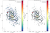 |
Fig. 4. Molecular hydrogen column density maps obtained via methods I and II. Left: high-res H2 column density map derived using all Herschel dust data employing method I with CO contours above the 3 and 6 σ level of the CO map shown in Fig. 1. Right: H2 column density map derived from SPIRE 250 μm map with method II. The circle to the lower left represents the resolution of 18.2″. |
Fitting β with a variable κ0 would result in different values for β. However, we avoid using the possibly wrong assumption of a fixed DGR. Instead, we establish the dependency of this parameter on galactocentric radius intrinsically6, which is integrated into our definition of κ0 (see Sect. 3.1). Given that β is correlated with star forming molecular gas (Tabatabaei et al. 2014), this correlation should still be maintained with a variable κ0. We therefore compare the above mentioned SED fits with the hydrogen column density maps with another fit over a small region around NGC 604, where we set β as a free fitting parameter while employing our variable κ0. This reproduces approximately the β map determined in Tabatabaei et al. (2014) (see Fig. D.1). The region covers both the atomic and molecular phases, with differences in β mostly below 0.2. The highest differences are located in the atomic phase, where our column density maps of molecular hydrogen are not affected anyway. However, the main drivers for the differences presumably arise from employing a one-component over a two-component modified blackbody fit, which includes a larger dataset. Additionally, different fitting parameters cause a non-unique solution for β. Nevertheless, as our simple fit reproduces approximately the same β values, we consider our approach to be self-consistent, despite the fact that the β map has been determined with a constant κ0.
3.5. Method II: Column density map from SPIRE 250 μm
The SPIRE 250 μm flux density map allows for the determination of the total hydrogen column density using Eq. (12) at an identical angular resolution of 18.2″ as in method I. This approach offers a simpler and more straightforward calculation and can be compared to the high-res map obtained with method I described in Sect. 3.4 and thus serves as a consistency check.
As for method I, we use the information of the β and κ0 maps at each pixel as described in Sect. 3.2 as well as the dust temperature map at each pixel from Tabatabaei et al. (2014), as shown in Fig. B.3. The resulting total hydrogen column density map is presented in Fig. 3 (right). Estimating the error of the dust column density map obtained with method II is not straightforward. Due to the utilisation of only one single band, the formal error introduced by the flux uncertainty is low. However, relying solely on one wavelength is inherently less reliable compared to a full SED fit across multiple wavelengths. Therefore, we can only presume that the uncertainty associated with the resulting NH map is of 30%.
Finally, we also subtract the H I column density (as for our high-res map obtained with method I) to arrive at an estimate of the molecular hydrogen column density shown in Fig. 4. Once more, determining a total error of the NH2 maps obtained using methods I and II is challenging. Here, the H I observations introduce an additional uncertainty. Nevertheless, the conversion of the line-integrated H I intensity into the H I column density incurs a small error. Consequently, we can conclude that our final H2 column density maps are accurate up to 20% for method I and 30% for method II.
4. Results and analysis
In this section, we start by presenting the probability distribution functions of the total hydrogen column density (N-PDFs) together with the H I N-PDF (Sect. 4.1). We then discuss the dust column density maps generated with both methods (Sect. 4.2) and compare them with the CO line-integrated map (Sect. 4.3). We finish by displaying and discussing the XCO factor map (Sect. 4.5).
4.1. Hydrogen column density PDFs
Generally, N-PDFs or density (ρ) PDFs are a powerful tool to describe the ISM and investigate its properties. They form the basis of star-formation theories (e.g. Padoan & Nordlund 2002; Hennebelle & Chabrier 2008; Federrath & Klessen 2012) and are commonly employed in dust and line observations for Galactic and extragalactic sources (e.g. Kainulainen et al. 2009; Froebrich & Rowles 2010; Hughes et al. 2013; Lombardi et al. 2015; Schneider et al. 2022). Simulations and theory showed that supersonic isothermal turbulence results in a log-normal distribution for the ρ- and N-PDF and self-gravity introduces a power-law tail (PLT) in the distribution at high densities (e.g. Vazquez-Semadeni 1994; Federrath et al. 2008; Kritsuk et al. 2011; Ballesteros-Paredes et al. 2011; Girichidis et al. 2014; Jaupart & Chabrier 2020).
We construct N-PDFs for the total hydrogen column density maps shown in Fig. 3 (with blue error bars calculated using Poisson statistics Schneider et al. 2015), for the dust-derived molecular hydrogen column density maps (Fig. 4), as well as for the CO map converted into NH2 with the derived XCO factor maps shown in Sect. 4.5.1 for the H I column density map (Fig. 1, left). In order to compare identical regions in the N-PDFs, we construct the N-PDFs considering only those pixels, which exhibit non-blanked values in Fig. 4. Figure 5 displays these N-PDFs in grey for the total hydrogen column density along with the dust-derived molecular hydrogen (in pink), the CO-to-NH2 (in blue and denoted as NH2(CO)) and the atomic hydrogen NHI-PDF (in green). Given that higher column density values result in smaller number statistics, and considering the limited resolution equivalent to 75 pc, we have beam-diluted column density values, leading to a plateau above ∼2 × 1022 cm−2 for the N-PDFs. Consequently, we opt to exclude these values from the analysis. A further increase in angular resolution would likely distinguish smaller areas, potentially preserving the power-law tail towards higher values (Schneider et al. 2015; Ossenkopf-Okada et al. 2016).
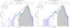 |
Fig. 5. N-PDFs obtained from the various column density maps. Left: N-PDF of the high-res NH column density map derived using all Herschel dust data employing method I only for non-blanked pixels of Fig. 4. Right: N-PDF of the NH column density map derived with method II for the same non-blanked pixels of Fig. 4. The green lines show the N-PDF of H I. Here, η is defined by |

Figure 5 suggests, by comparing the total (grey) and atomic (green) N-PDFs, that the majority of the column density is in the atomic phase, as the PDFs cover similar column density ranges. The NH I-PDF shows a sharp decrease towards higher column densities. Both peaks of the NH2-PDF and NH I-PDF are consistent with the peak of the total N-PDF, as adding the two peaks coincides with the total N-PDF peak. For values exceeding the H I column density (around 4 × 1021 cm−2), Fig. 5 indicates that these higher column densities are covered by the total N-PDF as well as the NH2 maps (derived from dust and CO). This suggests the presence of CO-bright molecular hydrogen. However, the border to CO-dark H2 gas cannot be determined from the N-PDFs. Both molecular PDFs exhibit a broader width compared to the H I and total column density PDFs, while the dust-derived NH2-PDF has the broadest width. This broadness may suggest the presence of CO-dark gas. Consistently, the derived NH2(CO)-PDF has a less broad width. The broad width of the dust-derived NH2-PDF also arises from subtracting H I from the total hydrogen column density, a phenomenon generally expected and discussed in Ossenkopf-Okada et al. (2016). In this study, ‘contamination’ of atomic and molecular gas along the line-of-sight was investigated, showing that a simple subtraction of a constant screen is a valid approach for galactic molecular clouds to correct for this effect, although it leads to broader PDFs and a shift of the peak column density to lower values. In the case of M33, the situation is more complex because in many sightlines multiple clouds may overlap within the beam. Note that this does not lead to several peaks in the PDF (Ossenkopf-Okada et al. 2016), but to a broader PDF distribution.
Considering the constructed N-PDFs for the whole region, as described in Appendix E and shown in Fig. E.1, discloses a different error tail for the N-PDFs from methods I and II. For both methods, the N-PDF shapes above ∼1020 cm−2, approximately the noise level of the map, are very similar. Below this value, a slight shoulder is visible, followed by a noise slope towards lower values for method I, which is absent for method II. This difference is likely due to the conversion via method II of the 250 μm map, which involves a conservative, possibly overly high, subtraction of the background emission, leading to the absence of a noise slope for low column densities. In method I, the impact of the background subtraction is less evident because here an SED fit is performed and the maps are subtracted to obtain a final high-res map. As highlighted in Palmeirim et al. (2013), the noise in this final map is slightly increased. However, due to this missing error tail from method II, we also see in the NH2-PDF in Fig. 5 (right and pink) a sharp decline towards lower column density.
In both N-PDFs, we observe an excess at high column densities, typically above 1022 cm−2. These data points in the context of the statistical analysis of the N-PDF exhibit significant uncertainty due to limited statistics and primarily stem from the most massive GMCs in M33. However, at such high column densities, we anticipate the onset of gravitational collapse of the whole GMC, or within larger clumps contained within them. In such cases, a PLT is expected to emerge, a phenomenon frequently observed in Milky Way studies (e.g. Lombardi et al. 2015; Stutz & Kainulainen 2015; Schneider et al. 2015, 2022), which links the PLT to self-gravity.
4.2. Comparison of dust-derived NH and NH2 maps
In the following subsections, we compare the NH maps and subsequently the NH2 maps derived with methods I and II.
4.2.1. Comparison of the NH maps
Figure 3 displays the total column density map ( ) derived using both methods I and II. Values exceeding the maximum threshold of 2.02 × 1022 cm−2 and 1.81 × 1022 cm−2 for methods I and II, respectively, are blanked. The GMC NGC604, the brightest region in M33, located at RA(2000) = 1h34m40s, Dec(2000) = 30°48′, was selected for this threshold. The mean column densities in both datasets are similar, with values of 1.06 × 1022 cm−2 and 1.23 × 1022 cm−2 for the NH maps of methods I and II, respectively. Across the entire disk, the NH maps shown in Fig. 3 exhibit a very similar morphology concerning the definition of the spiral arms, though method I produces slightly higher column densities in the spiral arms. Since dust has a lower optical depth at higher wavelengths, such as 500 μm, method I can potentially increase column density, as it gathers more information from dust emission than method II, which only uses the SPIRE map at 250 μm. Differences are primarily observed in the extent and smoothness of the diffuse inter-main spiral arm regions and the outer regions. method II appears to depict broader regions of gas in these areas of M33, while the map of method I exhibits higher local peaks, resulting in a more granular gas distribution. This discrepancy is most likely attributed to the implementation of the β parameter, which exhibits similar small-scale structures (as shown in Fig. B.2) and has a more pronounced impact on the final column density map for method I compared to method II, owing to differences in methodology (see Sect. 4.2.2). However, evaluating the authenticity of the small-scale structure is not straightforward. Additionally, we observe that in both NH maps, the gas within the western outer region of the galaxy (dashed grey ellipse in Fig. 6) reaches higher column densities compared to the eastern half of M33.
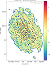 |
Fig. 6. (NH, Method I − NH, Method II)/NH, Method II difference map of the dust-derived total column density maps. The grey ellipse roughly delineates the area of enhanced emission observed in the western half of M33, as depicted in Figs. 3 (left) and 4 (left), in contrast to the eastern half. |
However, it is evident from the vast literature of CO maps of M33 that the galaxy comprises numerous GMCs and smaller molecular clouds, leading to the expectation of a rather non-uniform distribution, which is indeed reflected in the map produced using method I. Figure 6 displays the similarity between the NH maps obtained with methods I and II in a difference map. In the vicinity of the CO 3σ contours, method I tends to exhibit higher column densities. This transfers further into higher column densities concentrated within smaller regions in the outskirts and inter-main spiral regions, with a more rapid decline toward the edges of a GMC.
Those ‘peaks’ in the total hydrogen column density map obtained with method I can locally attain values of up to approximately 5 × 1021 cm−2. This observation aligns with what can be inferred from Fig. 3, where the map derived using method II presents a more uniform and smooth gas distribution, covering a broader area with lower “peak” values. The majority of the difference map shows values close to zero, indicating very similar NH maps.
4.2.2. Comparison of the NH2 maps
Upon subtracting the H I column density from both NH maps, as shown in Fig. 4, the spiral arms in the NH2 maps become even more distinct, as expected when GMCs form in the gravitational potential of the spiral arms from more diffuse H I gas. However, the diffuse gas (region outside the CO 3σ level) is only evident in the map obtained with method I. As for the NH2 maps, they have mean values of 2.95 × 1020 cm−2 for method I and 3.10 × 1020 cm−2 for method II.
While the morphology and overall magnitude of the NH2 maps generated within both methods are quite similar, the most significant contrast once again arises in the inter-main spiral and outer regions (see Fig. 4). In method II, the gas in the inter-main spiral region primarily results in a smoothly distributed gas pattern. In contrast, the map produced by method I reveals a more granular gas distribution, with higher local peaks in these inter-main spiral regions. These peaks reach values of approximately NH2 ≈ 3 × 1020 cm−2. The reason for this discrepancy lies in the role of the parameter β. In method II, κ0 is determined at 250 μm, so that the fraction in Eq. (12) is always 1. However, in method I, the situation is different. Here, all four bands spanning from 160 μm to 500 μm are utilised, leading to a fraction different from 1 in three out of four cases. Consequently, the value of β in the exponent significantly influences the resulting map. The maps produced by method I closely follow the morphology of the β emissivity index map in Fig. B.2 and contain additional information. As therefore β, which correlates with star formation and molecular gas Tabatabaei et al. (2014), is the main parameter causing this difference of molecular hydrogen gas seen in the dust-derived map of method I but not in the map of method II (which is unaffected by β) or CO, we tentatively attribute this partly to CO-dark gas.
4.2.3. Discussion of caveats and used methods
However, there is a caveat in our assumptions. We utilise the CO 2σ level to determine our dust absorption coefficient. Within this level, there is evidently CO emission spread across the entire disk of M33. As a result, the final dust absorption is overestimated, leading to a slight underestimation and hence a lower limit of the hydrogen column density (cf. Eq. (16)). Thus, there are a few regions, especially in the northern part of M33, where no NH2 is left within CO regions above 2σ. With an XCO factor of 1.8 × 1020 cm−2/(K km s−1) (see below) and the CO 2σ level, the H2 column density can reach values up to ∼1.3 × 1020 cm−2 in regions equal to and below the CO 2σ level. This is consistent with the mean column densities in the map for these regions, which fall below the specified threshold. Thus, we attribute this emission to originate from a non-changing κ0 which is introduced by the assumption. Furthermore, even including CO emission would still lack information regarding contributions from CO-dark H2 gas, which also plays a role in Eq. (15). Thus, trying to be as unbiased as possible regarding the CO emission and its CO-dark H2 gas problem, suggests our approach is reasonable to use in this regard. We note that for our determination of the dust absorption coefficient κ0, it is essential for the dust and gas to be well mixed. While this condition is certainly met in denser regions of molecular gas, it becomes less certain in the predominantly atomic phase.
Lastly, method II relies solely on information from a single Herschel map, while method I incorporates data from all four Herschel bands spanning from 160 μm to 500 μm, thus providing a more comprehensive dataset, particularly concerning cold GMCs. Furthermore, as the flux maps at wavelengths above 250 μm exhibit a lower dust optical depth, gaining more information from the dust emission, the column densities obtained with method I are more comprehensive. Furthermore, it encompasses additional information not only originating from the use of the various Herschel maps, but also from the β map. Method I is more elaborate to apply, but serves as a valuable tool for generating column density maps. Notably, it covers the information from the emissivity index to a greater extent compared to method II. Method II is a useful choice when only a single map is available and still produces satisfactory and comparable results. This method can be applied to any Herschel flux map; here we select 250 μm because it provides the best compromise between high angular resolution and detection of the cold gas component. Since the N-PDF of method I exhibits a noise tail, which is generally expected and absent in the N-PDF derived from method II, we consider method I to be the preferred option over method II, whenever the required data are available.
4.3. Comparison of the NH2 maps to the CO map
Comparing the dust-derived NH2 maps in Fig 4 with the CO line-integrated intensity map shown in Fig. 1 (right), all maps exhibit similar features with the spiral arms in both tracers. However, there are distinct differences. The emission of NH2 is more prominent in the inter-main spiral regions and extends further outward, whereas the emission of CO tends to be more concentrated locally in the inner regions within the main spiral arms. The extended column density observed in the NH2 maps may originate from CO-dark H2 gas, particularly near GMCs or in the outskirts of the galaxy, where the total hydrogen column densities are relatively lower. This is particularly true for the NH2 map derived using method I. A significant large-scale correlation between CO emission and H2 column densities exists (see Fig. 4 and the CO contour levels). However, this correlation does not hold consistently at smaller scales for cases of higher CO emission and both dust-derived NH2 from methods I and II. This discrepancy is observed in various regions of the disk.
Since we utilise CO(2 − 1) data, characterised by a higher critical density of ncrit = 1.1 × 104 cm−3 compared to CO(1 − 0) with a critical density of ncrit = 2.2 × 103 cm−3 (both at 20 K, Teng et al. 2022), a smaller region of CO(2 − 1) emission is excited. Therefore, detected GMCs may have smaller envelopes and a larger proportion of gas could be falsely attributed to CO-dark gas. However, this potential concern is likely mitigated by smoothing the CO line-integrated map to lower resolution, effectively addressing this limitation.
For data points above 3σ in CO, the Spearman coefficients are ρS = 0.4 and ρS = 0.49 for methods I and II, respectively. In contrast, the Pearson correlation yields slightly higher coefficients of ρP = 0.5 and ρP = 0.56 for methods I and II, respectively7. Both correlation coefficients show a positive but only moderate correlation. One possible explanation could be a too high κ0 value in the molecular phase, leading to an underestimation of the H2 column density. This suggests that the assumption of a uniform κ0 in both the atomic and molecular phases may be invalid in these regions, where the assumption treats κ0 as independent of density. This observation is also reflected in the Herschel maps presented in Fig. A.1, which display a better overall correlation between dust and CO emission, but a weaker correlation (to a smaller extent) in few regions between regions of high dust and high CO emission. In both cases, the coefficients show a positive and higher, but still only moderate correlation8. This disparity could potentially account for the lower correlation of especially higher CO emission with the molecular hydrogen column density derived from dust in some regions.
In summary, there are signs suggesting the potential existence of CO-dark H2 gas. Nonetheless, additional research is necessary to enhance our comprehension of the relationship and dynamics between CO and the dust tracers within M33. In Sect. 5 the results will be compared with the work of Braine et al. (2010b), who used a similar method to derive gas masses from the dust in M33.
4.4. The assumption of a non-changing κ0
The composition of dust, and hence the dust absorption coefficient, varies significantly with volume density. Environmental conditions influence the extent to which various elements deplete from the gas phase onto dust grains (Jenkins & Wallerstein 2017; Roman-Duval et al. 2021, 2022). Additionally, studies by Hirashita & Kobayashi (2013) and Aoyama et al. (2020) have revealed that the size distribution of dust grains is also affected by density. While theoretical models (Ossenkopf & Henning 1994; Jones 2018) propose an increasing dust opacity (κ) with density, empirical evidence from Clark et al. (2019a) suggests the opposite in nearby galaxies. They observed a decrease in κ with surface density, following a power-law index of −0.4. In a recent investigation by Clark et al. (2023), they presented compelling evidence for a changing κ following a power-law index of −0.4 with surface density in M33. Other studies (Bianchi et al. 2019, 2022) have indicated that the dust surface brightness per unit gas surface density increases with higher ISM surface densities and higher molecular-to-atomic gas ratios. A similar trend is observed for the dust luminosity per unit gas mass, implying that dust shows reduced emissivity in denser environments.
Thus, considering the correlation between the dust-derived hydrogen column density maps and the Herschel maps in comparison to the CO emission, it is reasonable to conclude that the assumption of a constant κ0 is valid only to a first-order approximation. However, since we lack the means to independently determine the column density before calculating κ0 in the molecular phase or vice versa, we cannot introduce a model that adjusts κ0 according to the density. Therefore, it is reasonable to consider our κ0 as a conservative estimate, representing a lower limit. In Clark et al. (2023), the variation in the dust-to-hydrogen ratio, attributed to a changing κ based on density, spans a range of approximately 2.5. Consequently, scaling κ0 with 2.5 in regions where CO exceeds 2σ leads to a column density showing a stronger correlation with CO emission. However, this approach does not account for a power-law relationship with density and can only provide a rough upper limit representation.
Other potential factors contributing to the observed variations could arise from variations in dust temperature. Lower dust temperature could lead to lower H2 column density and vice versa. However, as illustrated in Figs. B.3 and C.1, the shift in dust temperature from the dominant H I phase, where CO is below its 2σ level, to the molecular phase, where CO is above its 2σ threshold, is negligible. The β parameter may also contribute to explaining the variations with density. As shown in Tabatabaei et al. (2014), β correlates with star formation and the molecular phase; therefore, it may also change between the atomic and molecular phases. As depicted in Fig. B.2, the parameter β does not follow a strong, distinct pattern or shift in its value between the atomic and molecular phases (CO emission at the 2σ level). Its values fluctuate, being both low and high within the spiral arms, as well as in the regions between them and in the outer disk. In addition, β does not play a role in the map obtained with method II, as the reference wavelength in κg(ν) matches the wavelength of the SPIRE map used for method II. Since we still observe very similar variations in the dust-derived hydrogen column density map obtained via method II to CO emission, we can exclude β as the cause of these variations.
4.5. The XCO conversion factor
The XCO factor depends on several factors, including the ambient radiation field, metallicity, dust content and the evolutionary state of the galaxy in terms of star formation (cf. e.g. Bolatto et al. 2013). Notably, Offner et al. (2014) derived strong fluctuations in XCO depending on the ambient FUV flux. In regions with high FUV fields, CO can be readily photo-dissociated, making it a poor tracer for H2 (Kaufman et al. 1999; Kramer et al. 2004). Moreover, Israel (1997) suggested a linear correlation between XCO and the total infrared (TIR) luminosity, LTIR, over a wavelength range from 1 μm to 1 mm.
4.5.1. Determination of the XCO factor (ratio) map
With both a dust-derived H2 column density map and a CO integrated intensity map at our disposal, we can create an XCO factor (or ratio) map. This process involves dividing the values on a pixel-by-pixel basis in the dust-derived H2 column density maps by their corresponding values in the line-integrated CO(1 − 0) map. We apply a scaling factor of 0.8 based on the average CO(2 − 1)/CO(1 − 0) line ratio as discussed in (Druard et al. 2014) in order to obtain the CO(1 − 0) map9. This ratio typically ranges between ∼0.5 and ∼1.5.
The resulting XCO factor maps are visualised in Fig. 7. Both XCO maps trace the primary spiral arms of M33. The lowest values are around 1019 cm−2/(K km s−1) in the outer region, whereas the highest values are found in NGC604 and parts of the southern spiral arm, exceeding 1021 cm−2/(K km s−1). This observation is expected, as the lower CO emissions in the outer regions are predominantly optically thin, while the GMCs are optically thick, resulting in higher values.
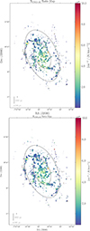 |
Fig. 7. XCO factor (ratio) maps of methods I and II. Determined as the dust-derived H2 column density over CO intensity determined at each position in both maps of M33 at 18.2″ and scaled with the |

Figure 7 also reveals distinct spatial variations of the XCO values within M33 in the two maps created via methods I and II. Although this variation is very large, a variability is expected, as the CO-to-H2 ratio naturally varies across the ISM of any galaxy which has been emphasised by Bolatto et al. (2013) and in recent studies (Ramambason et al. 2023; Chiang et al. 2024) as well.
In order to compare to the XCO values given for M33 in the literature, we derived an XCO value from a binned histogram. Additionally, we performed scatter plots and a radial line profile (in Appendix F) to systematically explore the potential radial dependence of XCO.
4.5.2. Analysis of the derived XCO factor
Histogram analysis. Figure 8 displays the histogram of the XCO conversion factor for all pixels exceeding the 3σ threshold of the data, as seen in the ratio maps in Fig. 7. Both distributions exhibit a slightly skewed Gaussian profile when viewed on a logarithmic scale. The standard deviation is large and close to the mean values for both methods, see Fig. 8. We performed a log-normal fit resulting in similar values of 2.1 × 1020 cm−2/(K km s−1) and 1.7 × 1020 cm−2/(K km s−1) for methods I and II, respectively.
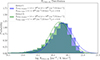 |
Fig. 8. Distribution of the XCO conversion factor from methods I and II in blue and green, respectively. The XCO(1 − 0) conversion factors of Fig. 7 and their standard deviations are given in the panel. A log-normal Gaussian fit is shown in the corresponding colours for methods I and II. |
Scatter plot analysis. The scatter plot analysis is presented in Fig. 9, exclusively for data points where CO emission exceeds the 3σ threshold. Data points within a galactocentric radius of 2 kpc are coloured in green and those beyond 2 kpc in purple. The ellipses outlining the data points used in the fit are presented in Fig. 7.
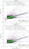 |
Fig. 9. Scatter plots of the dust-derived column density and CO(1 − 0) intensity determined for both maps of M33 at 18.2″. Grey data points correspond to those excluded in the fit. Top: scatter plot of method I. Bottom: scatter plot of method II. The estimated error of each individual data point is conservatively estimated to be 30%. |
A linear fit to all data points yields values of (1.6 ± 0.7)×1020 cm−2/(K km s−1) and (1.9 ± 0.7)×1020 cm−2/(K km s−1) for methods I and II, respectively. In the central region, relatively low values of 1.3(±0.4)−1.8(±0.4)×1020 cm−2/(K km s−1) from both methods are obtained for a galactocentric radius within 2 kpc. Focusing solely on the outermost points (beyond 4 kpc) provides values around 1.4(±0.9)−1.6(±1.1)×1020 cm−2/(K km s−1). These numbers do not result in a clear dependence of the XCO on the galactocentric radius.
The scatter is large and both correlation coefficients of Pearson and Spearman only yield moderate correlations for methods I and II (see Fig. 9). Especially, higher CO emission does not consistently correlate with an increased H2 column density (see also Sect. 4.3).
4.5.3. Discussion of the XCO factor
For simplicity, a single XCO factor is commonly employed in the literature. Previous studies (Gratier et al. 2010; Druard et al. 2014) have utilised a constant conversion factor of XCO(1 − 0) = 4 × 1020 cm−2/(K km s−1) for M33, which is twice the value employed for the Milky Way. This choice is based on the assumption that M33 possesses half the solar metallicity and that all other factors affecting the conversion factor such as the ambient radiation field or the optical depth of the CO emission lines, are similar to those of the Milky Way.
M33’s XCO relation to the Galactic value. However, when calculating the mean value of our XCO maps and conducting log-normal fitting, as well as a scatter plot analysis, we observe a contradiction to this assumption. The mean values appear to be below the Galactic value, and the scatter of the XCO values is within the same order as the mean values. Our findings are consistent with those of Ramambason et al. (2023), who noted that low-metallicity galaxies can display XCO factors as low as the Galactic value, coupled with an increasing dispersion of the conversion factor as metallicity decreases. Our results suggest a complex connection between the conversion factor and associated physical properties.
Braine et al. (2010b) determined an overall factor of XCO(1 − 0) = 2.1 × 1020 cm−2/(K km s−1) through a scatter plot analysis of dust column density and CO line intensity10, revealing also a value close to the Galactic value. While they as well find a lowered XCO value within 2 kpc of XCO(1 − 0) = 1.5 × 1020 cm−2/(K km s−1), their value beyond 2 kpc is higher with a value of XCO(1 − 0) = 2.9 × 1020 cm−2/(K km s−1). They argue that different regions within the galaxy, particularly the inner and outer areas, may exhibit distinct conversion factor values. Our results support this finding with regard to the scatter plot analysis (see Fig. 9). Figure 7 reveals lower values in the outskirts in comparison to the central region of M33.
This spatial variation does align with the expected relationship between the ambient radiation field and the XCO value (Bolatto et al. 2013), as the central region experiences a more intense radiation field in contrast to the outer regions along the galactocentric radius. A possible explanation is an increased optical depth of the CO emission towards the centre, as the optically thin CO emission correlates more effectively with H2 column density. This is supported by Druard et al. (2014), who observed broader line profiles of CO when successively approaching the centre.
Connection between enhanced metallicity and the XCO factor in the south. A large scatter in metallicity in M33 has been reported, which is unexplained by abundance uncertainties (Magrini et al. 2010). The peak in metallicity has been identified in the southern region of M33. Since the XCO factor is expected to decrease with increasing metallicity, we should observe lowered XCO values in the southern region, assuming no substantial variations in other influencing factors of XCO, such as the ambient radiation field. However, our observations do not indicate a significantly lower XCO factor in this area. We derive a mean value of 1.60 × 1020 cm−2/(K km s−1) for the northern part and 1.96 × 1020 cm−2/(K km s−1) for the southern part, respectively, using method I. For method II, these values are slightly lower, at 1.43 × 1020 cm−2/(K km s−1) for the northern part and 1.68 × 1020 cm−2/(K km s−1) for the southern part, respectively. Although the values in the southern region are marginally higher, they still fall within the broad standard variation, thereby lacking the statistical power to account for the observed small difference or a systematic increase in metallicity in the southern region.
While the variability of the XCO factor in general can be attributed to fluctuations in metallicity within M33, variations in dust content and star formation rates also play a role (Bolatto et al. 2013). Moreover, the XCO factor is further influenced by the ambient radiation field. For instance, if we consider a scenario where all other factors remain constant but the radiation field decreases with increasing galactocentric radius, the XCO factor would be expected to decrease correspondingly. Nevertheless, the intricate interplay of these processes, as discussed earlier, results in a complex relationship where all factors concurrently influence the XCO factor. Investigating and differentiating the individual contributions of these processes to the observed variations in the XCO factor are beyond the scope of this study.
Caveats of the methods and consequences of the results. While the scatter fit in Fig. 9 shows a potential correlation between CO emission and H2 column density, the log-normal fit and histogram presented in Fig. 8 illustrate the distribution of the previously computed XCO factor and the frequency of different values. Moreover, the radial profile in Appendix F is constructed by averaging the data points within a distance of 100 pc along the galactocentric radius. Each of those bins exhibit a higher scatter in the XCO values compared to all the pixels in the XCO maps. Furthermore, their contribution on the overall average decreases as the galactocentric radius increases, given that they consist of a significantly smaller number of data points in comparison to the entire dataset. This helps elucidate the difference in the results obtained from the methods used to determine the XCO factor.
We emphasise that the range of the XCO factor (Fig. 8) is broad. For all methods used to calculate the XCO factor, the standard deviation is close to the determined mean value, indicating a substantial and wide variation of this parameter. Consequently, assuming a constant XCO factor, as is often practised in other studies, can lead to results that differ by an order of magnitude and are insufficient for ensuring reliable outcomes.
5. Discussion and comparison of the H2 column density maps with other studies
In this section, we present our results for the construction of hydrogen column density maps of M33 with the two different methods presented above in context with other studies such as those of Braine et al. (2010b), Tabatabaei et al. (2014), Gratier et al. (2017), Clark et al. (2021). An overview of the parameters used and their characteristics is provided in Table 1.
Parameters used to calculate column or surface densities of molecular hydrogen in several studies of M33.
Braine et al. (2010b) made no assumptions regarding the XCO factor and a variable dust absorption coefficient κ0 (along with a variable dust-to-gas ratio) is determined similar to our approach. However, they only employ a fixed emissivity index β throughout the whole disk and a fixed κ0 inside the galactocentric radius of 4 kpc, while in our case, κ0 and β vary on a pixel-by-pixel basis throughout the disk. The molecular hydrogen column density map of Braine et al. (2010b) has a lower angular resolution (approximately 40″) due to the application of the simple canonical SED fit to all Herschel flux maps. It is also worth noting that the CO map used by Braine et al. (2010b) was incomplete and covers an area of approximately 2/3 of the final map of Druard et al. (2014) used here.
The primary focus of the study by Tabatabaei et al. (2014) lies on the emissivity index. For this purpose, the absolute value of the column density is not considered, and hence, they use a fixed dust absorption coefficient that does not bias the fitting of the emissivity index β.
Gratier et al. (2017) employed an H I dataset from Gratier et al. (2010) to derive the dust absorption coefficient in a manner similar to Braine et al. (2010b) and our present study for the purpose of calculating the total column density of hydrogen. They also utilised the same IRAM CO(2 − 1) map as we did for this purpose. However, the emissivity index β is only used with a radial dependence, rather than on a pixel-by-pixel basis. They solved for an XCO factor and a gas-to-dust ratio (GDR) in their analysis of the molecular content, presenting radial trends. The angular resolution of their maps is approximately 25″ or about 100 pc, due to the utilisation of a canonical one-component modified blackbody SED fit.
Clark et al. (2021) employed a broken-emissivity modified blackbody model to account for the sub-millimetre excess, which arises relative to a canonical β = 2 at longer wavelengths in the Rayleigh-Jeans regime, specifically around the 500 μm Herschel data point. They determined different values of β for this purpose. However, this variation in β only affects the data points where the sub-millimetre excess is modelled and is not on a pixel-by-pixel basis. They note that the sub-millimetre excess for M33 is relatively small (Clark et al. 2021). For the dust-derived column density map of atomic hydrogen, they used a fixed dust absorption coefficient, with the value determined for the Large Magellanic Cloud. Additionally, they applied a fixed XCO factor using the Galactic value. Both atomic and molecular phases were combined to produce a total surface density map, but this approach does not account for CO-dark H2 gas. The resulting map has the same resolution as the Herschel 500 μm map, approximately 40″ or about 150 pc.
Despite of the differences in the calculation of column densities, all final maps as listed in Table 1 agree to within the same order of magnitude. In comparison to other studies, our methods have the advantage that the hydrogen column density maps are determined on a pixel-by-pixel basis, providing the highest angular resolution among them.
6. Conclusion and summary
We have generated dust-derived hydrogen column density maps using Herschel flux data of M33 with two methods. Method I follows the procedure outlined by Palmeirim et al. (2013) and employs an SED fit to the 160 μm to 500 μm data. It benefits from combining additional Herschel data at longer wavelengths, where the dust typically has lower optical depths. Method II transforms the 250 μm SPIRE map into a hydrogen column density. For both maps we incorporated the emissivity index β map and a temperature map of the cold dust component from Tabatabaei et al. (2014). With the H I map of Gratier et al. (2010) in addition, we calculated a variable κ0 map on a pixel-by-pixel basis, thereby providing all parameters of the dust opacity law for each pixel. This approach circumvents the need for assumptions regarding the XCO factor, dust-to-gas ratio (such as constant values for both) or the dependency on the galactocentric radius. The variability and dependencies of these factors are intrinsically encompassed through our computation of κ0 and the utilisation of the provided β map. We note that the DGR is inherently included in our definition of κ0. Subsequently, we subtracted the H I contribution from the two NH maps by transforming the VLA H I integrated intensity map to an H I column density map to create maps of molecular gas columndensities, NH2.
Our column density maps of total and molecular hydrogen are consistent in the order of magnitude compared to other studies (Braine et al. 2010b; Gratier et al. 2017; Clark et al. 2021). Overall, the results obtained from method II confirm those derived by employing method I. Nevertheless, the results obtained using method I demonstrate a rise in H2 column densities, manifesting as granular gas distributions in M33’s inter-main spiral and outer regions, which we cautiously propose may stem partially from CO-dark gas. Both methods display comparable hydrogen column density N-PDFs. We tentatively fit log-normal distributions at low column densities and a power-law tail at high column densities, which may indicate gravitational collapse of the dense gas in the GMCs. The high-column density part of the total hydrogen N-PDF likely arises from CO-bright H2 gas, since the Only beyond a galactocentric radius of 4 kpc. molecular N-PDFs from dust and CO cover the same range. The parts of CO-dark gas in the N-PDFs cannot be determined. We caution that the interpretation of extragalatic N-PDFs is challenging due to the sampling of many molecular clouds along the line-of-sight11.
Furthermore, our investigation of the XCO factor leads to consistent results falling within the standard deviation for each method. Remarkably, the XCO factor is about half as large as the value observed in the Milky Way when considering the result from the scatter fit. This stands in contrast to prior assumptions claiming that the XCO factor should be twice that of the Galactic value (Druard et al. 2014; Gratier et al. 2017). Notably, the dispersion of the XCO factor can extend beyond one order of magnitude, rendering the assumption of a constant XCO factor even more questionable.
To conclude, we demonstrate the robustness and applicability of method I in producing reliable results using extragalactic data, enabling us to present a previously unachieved and unprecedented NH and NH2 map of M33 with a remarkably improved angular resolution of 18.2″. This map reflects the dependency on important influencing factors such as the dust-to-gas ratio, dust opacity law, and the XCO factor on a pixel-by-pixel basis. In a follow-up paper (in prep.), we apply Dendrograms on this column density map of method I to extract cloud structures. This will enable us to derive and explore various physical properties of these clouds, including number density, mass, size, mass-size relation, and mass spectra. By comparing our findings with existing Milky Way data, we aspire to provide a more comprehensive understanding of cloud properties and dynamics across diverse environments.
Data availability
All final data products are available at the CDS via anonymous ftp to https://cdsarc.cds.unistra.fr ( 130.79.128.5 ) or via https://cdsarc.cds.unistra.fr/viz-bin/cat/J/A+A/688/A171
Brent’s method (Brent 1973) is an iterative approach for determining a root, combining the bisection method, the secant method, and the inverse quadratic interpolation. From the combination of these techniques, Brent’s method has a faster convergence rate and greater robustness compared to using each individual method alone.
The Spearman correlation coefficient, which is applicable to any monotonic relationship (linear and non-linear) and data that do not necessarily need to be normally distributed, is more robust against outliers than the Pearson correlation coefficient. Since the Spearman correlation coefficient works well for both linear and non-linear relations, it therefore does not distinguish between them. In contrast, the Pearson correlation requires normally distributed data with a strict linear relation.
For data points above 3σ in CO, the Spearman coefficients are 0.61, 0.66, 0.65, and 0.60 for the PACS 160 μm and SPIRE 250 μm, 350 μm, 500 μm maps, respectively. In contrast, the Pearson correlation yields slightly higher coefficients of 0.66, 0.72, 0.71, and 0.64 for the PACS 160 μm and SPIRE 250 μm, 350 μm, 500 μm maps, respectively.
The background is that the virial theorem was originally applied to determine total mass from the velocity dispersion of a cloud and correlated to the integrated 12CO line intensity (Bolatto et al. 2013) to obtain XCO. This approach was suitable even for the optically thick case of CO lines.
Braine et al. (2010b) use a line ratio of  as determined in Gratier et al. (2010), who used the incomplete CO map from the IRAM Large Program. We use, however, the determined line ratio of
  by Druard et al. (2014), who employed the full CO map of M33.
Acknowledgments
E.K. and N.S. acknowledge support from the FEEDBACK-plus project that is supported by the BMWI via DLR, Project Number 50OR2217. E.K. acknowledges support by the BMWI via DLR, project number 50OK2101. S.K. acknowledges support from the Orion-Legacy project that is supported by the BMWI via DLR, project number 50OR2311. This work was supported by the Collaborative Research Center 1601 (SFB 1601 sub-projects A6 and B2) funded by the Deutsche Forschungsgemeinschaft (DFG, German Research Foundation) – 500700252.
References
- André, P., Men’shchikov, A., Bontemps, S., et al. 2010, A&A, 518, L102 [NASA ADS] [CrossRef] [EDP Sciences] [Google Scholar]
- Aoyama, S., Hirashita, H., & Nagamine, K. 2020, MNRAS, 491, 3844 [NASA ADS] [Google Scholar]
- Ballesteros-Paredes, J., Vázquez-Semadeni, E., Gazol, A., et al. 2011, MNRAS, 416, 1436 [NASA ADS] [CrossRef] [Google Scholar]
- Bianchi, S., Casasola, V., Baes, M., et al. 2019, A&A, 631, A102 [NASA ADS] [CrossRef] [EDP Sciences] [Google Scholar]
- Bianchi, S., Casasola, V., Corbelli, E., et al. 2022, A&A, 664, A187 [NASA ADS] [CrossRef] [EDP Sciences] [Google Scholar]
- Bigiel, F., Leroy, A. K., Walter, F., et al. 2011, ApJ, 730, L13 [NASA ADS] [CrossRef] [Google Scholar]
- Bloemen, J. B. G. M., Strong, A. W., Mayer-Hasselwander, H. A., et al. 1986, A&A, 154, 25 [NASA ADS] [Google Scholar]
- Bohlin, R. C., Savage, B. D., & Drake, J. F. 1978, ApJ, 224, 132 [Google Scholar]
- Bolatto, A. D., Wolfire, M., & Leroy, A. K. 2013, ARA&A, 51, 207 [CrossRef] [Google Scholar]
- Boquien, M., Calzetti, D., Kramer, C., et al. 2010, A&A, 518, L70 [NASA ADS] [CrossRef] [EDP Sciences] [Google Scholar]
- Boquien, M., Calzetti, D., Combes, F., et al. 2011, AJ, 142, 111 [CrossRef] [Google Scholar]
- Boquien, M., Calzetti, D., Aalto, S., et al. 2015, A&A, 578, A8 [NASA ADS] [CrossRef] [EDP Sciences] [Google Scholar]
- Borchert, E. M. A., Walch, S., Seifried, D., et al. 2022, MNRAS, 510, 753 [Google Scholar]
- Boselli, A., Ciesla, L., Cortese, L., et al. 2012, A&A, 540, A54 [NASA ADS] [CrossRef] [EDP Sciences] [Google Scholar]
- Braine, J., Gratier, P., Kramer, C., et al. 2010a, A&A, 520, A107 [NASA ADS] [CrossRef] [EDP Sciences] [Google Scholar]
- Braine, J., Gratier, P., Kramer, C., et al. 2010b, A&A, 518, L69 [NASA ADS] [CrossRef] [EDP Sciences] [Google Scholar]
- Braine, J., Gratier, P., Contreras, Y., Schuster, K. F., & Brouillet, N. 2012a, A&A, 548, A52 [NASA ADS] [CrossRef] [EDP Sciences] [Google Scholar]
- Braine, J., Gratier, P., Kramer, C., et al. 2012b, A&A, 544, A55 [NASA ADS] [CrossRef] [EDP Sciences] [Google Scholar]
- Brent, R. P. 1973, Algorithms for Minimization without Derivatives (Englewood Cliffs: Prentice-Hall) [Google Scholar]
- Buchbender, C., Kramer, C., Gonzalez-Garcia, M., et al. 2013, A&A, 549, A17 [NASA ADS] [CrossRef] [EDP Sciences] [Google Scholar]
- Casey, C. M., Chapman, S. C., Smail, I., et al. 2011, MNRAS, 411, 2739 [NASA ADS] [CrossRef] [Google Scholar]
- Chapin, E. L., Chapman, S. C., Coppin, K. E., et al. 2011, MNRAS, 411, 505 [Google Scholar]
- Chiang, I.-D., Sandstrom, K. M., Chastenet, J., et al. 2024, ApJ, 964, 18 [NASA ADS] [CrossRef] [Google Scholar]
- Clark, C. J. R., De Vis, P., Baes, M., et al. 2019a, MNRAS, 489, 5256 [NASA ADS] [CrossRef] [Google Scholar]
- Clark, P. C., Glover, S. C. O., Ragan, S. E., & Duarte-Cabral, A. 2019b, MNRAS, 486, 4622 [Google Scholar]
- Clark, C. J. R., Roman-Duval, J. C., Gordon, K. D., Bot, C., & Smith, M. W. L. 2021, ApJ, 921, 35 [CrossRef] [Google Scholar]
- Clark, C. J. R., Roman-Duval, J. C., Gordon, K. D., et al. 2023, ApJ, 946, 42 [NASA ADS] [CrossRef] [Google Scholar]
- Cormier, D., Madden, S. C., Lebouteiller, V., et al. 2014, A&A, 564, A121 [NASA ADS] [CrossRef] [EDP Sciences] [Google Scholar]
- Crockett, N. R., Garnett, D. R., Massey, P., & Jacoby, G. 2006, ApJ, 637, 741 [NASA ADS] [CrossRef] [Google Scholar]
- den Brok, J. S., Bigiel, F., Chastenet, J., et al. 2023, A&A, 676, A93 [NASA ADS] [CrossRef] [EDP Sciences] [Google Scholar]
- Druard, C., Braine, J., Schuster, K. F., et al. 2014, A&A, 567, A118 [NASA ADS] [CrossRef] [EDP Sciences] [Google Scholar]
- Elia, D., Strafella, F., Dib, S., et al. 2018, MNRAS, 481, 509 [Google Scholar]
- Federrath, C., & Klessen, R. S. 2012, ApJ, 761, 156 [Google Scholar]
- Federrath, C., Klessen, R. S., & Schmidt, W. 2008, ApJ, 688, L79 [NASA ADS] [CrossRef] [Google Scholar]
- Froebrich, D., & Rowles, J. 2010, MNRAS, 406, 1350 [NASA ADS] [Google Scholar]
- Gardan, E., Braine, J., Schuster, K. F., Brouillet, N., & Sievers, A. 2007, A&A, 473, 91 [NASA ADS] [CrossRef] [EDP Sciences] [Google Scholar]
- Girichidis, P., Konstandin, L., Whitworth, A. P., & Klessen, R. S. 2014, ApJ, 781, 91 [CrossRef] [Google Scholar]
- Gratier, P., Braine, J., Rodriguez-Fernandez, N. J., et al. 2010, A&A, 522, A3 [NASA ADS] [CrossRef] [EDP Sciences] [Google Scholar]
- Gratier, P., Braine, J., Rodriguez-Fernandez, N. J., et al. 2012, A&A, 542, A108 [NASA ADS] [CrossRef] [EDP Sciences] [Google Scholar]
- Gratier, P., Braine, J., Schuster, K., et al. 2017, A&A, 600, A27 [NASA ADS] [CrossRef] [EDP Sciences] [Google Scholar]
- Hennebelle, P., & Chabrier, G. 2008, ApJ, 684, 395 [Google Scholar]
- Hirashita, H., & Kobayashi, H. 2013, Earth Planets Space, 65, 1083 [NASA ADS] [CrossRef] [Google Scholar]
- Hughes, A., Meidt, S. E., Colombo, D., et al. 2013, ApJ, 779, 46 [NASA ADS] [CrossRef] [Google Scholar]
- Israel, F. P. 1997, A&A, 328, 471 [NASA ADS] [Google Scholar]
- Jaupart, E., & Chabrier, G. 2020, ApJ, 903, L2 [NASA ADS] [CrossRef] [Google Scholar]
- Jenkins, E. B., & Wallerstein, G. 2017, ApJ, 838, 85 [NASA ADS] [CrossRef] [Google Scholar]
- Jones, A. P. 2018, arXiv e-prints [arXiv:1804.10628] [Google Scholar]
- Juvela, M., Demyk, K., Doi, Y., et al. 2015a, A&A, 584, A94 [NASA ADS] [CrossRef] [EDP Sciences] [Google Scholar]
- Juvela, M., Ristorcelli, I., Marshall, D. J., et al. 2015b, A&A, 584, A93 [NASA ADS] [CrossRef] [EDP Sciences] [Google Scholar]
- Kainulainen, J., Beuther, H., Henning, T., & Plume, R. 2009, A&A, 508, L35 [NASA ADS] [CrossRef] [EDP Sciences] [Google Scholar]
- Karachentsev, I. D., Karachentseva, V. E., Huchtmeier, W. K., & Makarov, D. I. 2004, AJ, 127, 2031 [Google Scholar]
- Kaufman, M. J., Wolfire, M. G., Hollenbach, D. J., & Luhman, M. L. 1999, ApJ, 527, 795 [Google Scholar]
- Könyves, V., André, P., Men’shchikov, A., et al. 2015, A&A, 584, A91 [Google Scholar]
- Kramer, C., Jakob, H., Mookerjea, B., et al. 2004, A&A, 424, 887 [NASA ADS] [CrossRef] [EDP Sciences] [Google Scholar]
- Kramer, C., Buchbender, C., Xilouris, E. M., et al. 2010, A&A, 518, L67 [NASA ADS] [CrossRef] [EDP Sciences] [Google Scholar]
- Kramer, C., Nikola, T., Anderl, S., et al. 2020, A&A, 639, A61 [NASA ADS] [CrossRef] [EDP Sciences] [Google Scholar]
- Kritsuk, A. G., Norman, M. L., & Wagner, R. 2011, ApJ, 727, L20 [NASA ADS] [CrossRef] [Google Scholar]
- Krügel, E. 2003, The physics of Interstellar Dust (Bristol, UK: The Institute of Physics) [CrossRef] [Google Scholar]
- Krügel, E., & Siebenmorgen, R. 1994, A&A, 288, 929 [Google Scholar]
- Larson, R. B. 1969, MNRAS, 145, 271 [Google Scholar]
- Leroy, A. K., Bolatto, A., Gordon, K., et al. 2011, ApJ, 737, 12 [Google Scholar]
- Leroy, A. K., Walter, F., Sandstrom, K., et al. 2013, AJ, 146, 19 [Google Scholar]
- Lombardi, M., Alves, J., & Lada, C. J. 2015, A&A, 576, L1 [NASA ADS] [CrossRef] [EDP Sciences] [Google Scholar]
- Madden, S. C., Cormier, D., Hony, S., et al. 2020, A&A, 643, A141 [NASA ADS] [CrossRef] [EDP Sciences] [Google Scholar]
- Magrini, L., Stanghellini, L., & Villaver, E. 2009, ApJ, 696, 729 [NASA ADS] [CrossRef] [Google Scholar]
- Magrini, L., Stanghellini, L., Corbelli, E., Galli, D., & Villaver, E. 2010, A&A, 512, A63 [NASA ADS] [CrossRef] [EDP Sciences] [Google Scholar]
- Nguyen-Luong, Q., Nguyen, H. V. V., Motte, F., et al. 2016, ApJ, 833, 23 [NASA ADS] [CrossRef] [Google Scholar]
- Offner, S. S. R., Bisbas, T. G., Bell, T. A., & Viti, S. 2014, MNRAS, 440, L81 [NASA ADS] [CrossRef] [Google Scholar]
- Ossenkopf, V., & Henning, T. 1994, A&A, 291, 943 [NASA ADS] [Google Scholar]
- Ossenkopf-Okada, V., Csengeri, T., Schneider, N., Federrath, C., & Klessen, R. S. 2016, A&A, 590, A104 [NASA ADS] [CrossRef] [EDP Sciences] [Google Scholar]
- Padoan, P., & Nordlund, Å. 2002, ApJ, 576, 870 [NASA ADS] [CrossRef] [Google Scholar]
- Palmeirim, P., André, P., Kirk, J., et al. 2013, A&A, 550, A38 [NASA ADS] [CrossRef] [EDP Sciences] [Google Scholar]
- Pedregosa, F., Varoquaux, G., Gramfort, A., et al. 2011, J. Mach. Learn. Res., 12, 2825 [Google Scholar]
- Pineda, J. L., Langer, W. D., Velusamy, T., & Goldsmith, P. F. 2013, A&A, 554, A103 [CrossRef] [EDP Sciences] [Google Scholar]
- Pineda, J. L., Langer, W. D., & Goldsmith, P. F. 2014, A&A, 570, A121 [NASA ADS] [CrossRef] [EDP Sciences] [Google Scholar]
- Putman, M. E., Peek, J. E. G., Muratov, A., et al. 2009, ApJ, 703, 1486 [NASA ADS] [CrossRef] [Google Scholar]
- Ramambason, L., Lebouteiller, V., Madden, S. C., et al. 2023, A&A, 681, A14 [Google Scholar]
- Regan, M. W., & Vogel, S. N. 1994, ApJ, 434, 536 [NASA ADS] [CrossRef] [Google Scholar]
- Relaño, M., Verley, S., Pérez, I., et al. 2013, A&A, 552, A140 [NASA ADS] [CrossRef] [EDP Sciences] [Google Scholar]
- Relaño, M., Kennicutt, R., Lisenfeld, U., et al. 2016, A&A, 595, A43 [NASA ADS] [CrossRef] [EDP Sciences] [Google Scholar]
- Relaño, M., De Looze, I., Kennicutt, R. C., et al. 2018, A&A, 613, A43 [NASA ADS] [CrossRef] [EDP Sciences] [Google Scholar]
- Robitaille, J. F., Motte, F., Schneider, N., Elia, D., & Bontemps, S. 2019, A&A, 628, A33 [NASA ADS] [CrossRef] [EDP Sciences] [Google Scholar]
- Rohlfs, K., & Wilson, T. L. 1996, Tools of Radio Astronomy (Springer Berlin, Heidelberg) [CrossRef] [Google Scholar]
- Röllig, M., Ossenkopf, V., Jeyakumar, S., Stutzki, J., & Sternberg, A. 2006, A&A, 451, 917 [Google Scholar]
- Roman-Duval, J., Jenkins, E. B., Tchernyshyov, K., et al. 2021, ApJ, 910, 95 [NASA ADS] [CrossRef] [Google Scholar]
- Roman-Duval, J., Jenkins, E. B., Tchernyshyov, K., et al. 2022, ApJ, 928, 90 [NASA ADS] [CrossRef] [Google Scholar]
- Rosolowsky, E. W., Pineda, J. E., Kauffmann, J., & Goodman, A. A. 2008, ApJ, 679, 1338 [Google Scholar]
- Roussel, H. 2013, PASP, 125, 1126 [Google Scholar]
- Sandstrom, K. M., Leroy, A. K., Walter, F., et al. 2013, ApJ, 777, 5 [Google Scholar]
- Schneider, N., Csengeri, T., Klessen, R. S., et al. 2015, A&A, 578, A29 [NASA ADS] [CrossRef] [EDP Sciences] [Google Scholar]
- Schneider, N., Ossenkopf-Okada, V., Clarke, S., et al. 2022, A&A, 666, A165 [NASA ADS] [CrossRef] [EDP Sciences] [Google Scholar]
- Sodroski, T. J., Odegard, N., Dwek, E., et al. 1995, ApJ, 452, 262 [Google Scholar]
- Spilker, A., Kainulainen, J., & Orkisz, J. 2021, A&A, 653, A63 [NASA ADS] [CrossRef] [EDP Sciences] [Google Scholar]
- Starck, J. L., Aghanim, N., & Forni, O. 2004, A&A, 416, 9 [NASA ADS] [CrossRef] [EDP Sciences] [Google Scholar]
- Stutz, A. M., & Kainulainen, J. 2015, A&A, 577, L6 [NASA ADS] [CrossRef] [EDP Sciences] [Google Scholar]
- Tabatabaei, F. S., Braine, J., Xilouris, E. M., et al. 2014, A&A, 561, A95 [NASA ADS] [CrossRef] [EDP Sciences] [Google Scholar]
- Tacconi, L. J., Genzel, R., Saintonge, A., et al. 2018, ApJ, 853, 179 [Google Scholar]
- Teng, Y.-H., Sandstrom, K. M., Sun, J., et al. 2022, ApJ, 925, 72 [NASA ADS] [CrossRef] [Google Scholar]
- Vazquez-Semadeni, E. 1994, ApJ, 423, 681 [Google Scholar]
- Veltchev, T. V., Ossenkopf-Okada, V., Stanchev, O., et al. 2018, MNRAS, 475, 2215 [Google Scholar]
- Verley, S., Corbelli, E., Giovanardi, C., & Hunt, L. K. 2010a, A&A, 510, A64 [NASA ADS] [CrossRef] [EDP Sciences] [Google Scholar]
- Verley, S., Relaño, M., Kramer, C., et al. 2010b, A&A, 518, L68 [NASA ADS] [CrossRef] [EDP Sciences] [Google Scholar]
- Whitworth, A., & Summers, D. 1985, MNRAS, 214, 1 [Google Scholar]
- Willner, S. P., & Nelson-Patel, K. 2002, ApJ, 568, 679 [CrossRef] [Google Scholar]
- Wolfire, M. G., Hollenbach, D., & McKee, C. F. 2010, ApJ, 716, 1191 [Google Scholar]
- Xilouris, E. M., Tabatabaei, F. S., Boquien, M., et al. 2012, A&A, 543, A74 [NASA ADS] [CrossRef] [EDP Sciences] [Google Scholar]
- Yahia, H., Schneider, N., Bontemps, S., et al. 2021, A&A, 649, A33 [NASA ADS] [CrossRef] [EDP Sciences] [Google Scholar]
Appendix A: Background Correction for Herschel Fluxes and Herschel Flux Maps
Table A.1 shows the mean, rms, minimum and maximum intensity of the background for the Herschel dust maps at wavelength 160 μm, 250 μm, 350 μm and 500 μm. The mean values have been subtracted from each corresponding dust map prior to processing into the high-res column density map. Figure A.1 shows these Herschel maps at their original resolution in MJy sr−1. We note the different scales in the colour bars for the 160 μm map compared to the other maps.
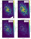 |
Fig. A.1. Herschel flux maps in MJy sr−1 at the four observing wavelengths with overlaid CO contours at 3σ, 6σ, and 12σ. |
Basic statistics of the Herschel dust maps.
Appendix B: κ0 map before filling and complementary maps
KNNImputer uses data from k-Nearest neighbouring pixels for computing their mean and substituting missing values with this information. It employs the Euclidean distance metric to assess the proximity of neighbouring data points, assigning equal importance to each. Assuming that there are no significant variations in the dust characteristics between the atomic and molecular phases of hydrogen, the KNNImputer method fills the gaps in the κ0 map by considering k = 5 pixels located at the boundaries of the cavities depicted in Fig. B.1, where the CO emission reaches the 2σ threshold. For comparison, the κ0 map before filling with KNNImputer is shown in Fig. B.1. The β and temperature maps of Tabatabaei et al. (2014) used to determine the κ0 map are shown in Figs. B.2 and B.3
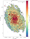 |
Fig. B.2. Emissivity index β map from Tabatabaei et al. (2014). CO contours at the 2σ level are overlaid on the map. |
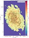 |
Fig. B.3. Temperature map obtained by Tabatabaei et al. (2014) used in both methods and in the determination of κ0. |
Appendix C: Temperature maps
Two temperature maps at the corresponding resolution of the SPIRE 350 μm and 500 μm maps are obtained from the SED fits, which are shown in Fig. C.1. The colour temperature obtained using the flux ratio at the corresponding resolution of the SPIRE 250 μm map was not used because using this map yields a column density map with higher noise in the outskirts of the galaxy. The requirements to use the flux ratio are anyway not fulfilled, since both wavelengths are in the Rayleigh-Jeans limit, where the dust temperature Td will tend to cancel out due to Bν(Td)∝Td. Additionally, the dust temperature should be uniform in the source and observations with two different frequencies should measure the same object. When the source is extended compared to the telescope beam and the observations have different spatial resolutions (as in our case), it is not trivial to fulfil this requirement.
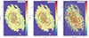 |
Fig. C.1. Temperature maps obtained and used within both methods. Left: Temperature map at 500 μm obtained with method I. Middle: Temperature map at 350 μm obtained with method I. Right: Colour temperature map at 250 μm obtained with method I using the flux ratio of SPIRE 250 μm and PACS 160 μm. Note, this map was not used. |
Although the requirements for determining the colour ratio are not fully met, the result is remarkably good, as can be seen in Fig. C.1, bottom left. However, higher noise features are still produced in the outskirts when using this map. We therefore decided to use the temperature map provided by Tabatabaei et al. (2014) shown in Fig. B.3.
All temperature maps show a gradient declining from the centre to the outskirts of the disk. While the colour temperature map obtained with the flux ratio shows the highest temperatures and an unsmooth, bumpy distribution (due to the not fully met requirements), the two temperature maps obtained with the SED fits show a much smoother distribution with lower higher temperatures in the centre. The temperature map obtained at the corresponding resolution of the SPIRE 350 μm map has higher local values compared to the map at 500 μm. Comparing these to the map from Tabatabaei et al. (2014) shown in Fig. B.3, the latter has a similar gradient. The main difference is that the higher values spread over a larger area, whereas the local maxima are lower compared to especially the map at the corresponding 350 μm. However, all maps exhibit a mean value of around ∼ 20 K.
Appendix D: Consistency of the emissivity index
To demonstrate that using a variable κ0 will not cause inconsistencies when employing a variable β map, which has been determined with a constant κ0, we present in Fig. D.1 a simple fit of β with our variable κ0 map and compare it with the β map used by Tabatabaei et al. (2014), as described in Sect. 3. The fitted region around NGC604, shown in Fig. D.1, includes areas of both the atomic and molecular phases. Most differences, especially in the molecular phase, which is most important for the follow-up paper, are small.
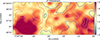 |
Fig. D.1. β map obtained by Tabatabaei et al. (2014) around NGC604 including areas of atomic and molecular phases. The contour lines represent the differences between our additional fit and the one of Tabatabaei et al. (2014), with values of −0.1, 0, 0.1 and 0.2 shown in white, red, blue and grey, respectively. |
Appendix E: Hydrogen column density PDFs
We construct N-PDFs for the whole total hydrogen column density maps shown in Fig. 3. Figure E.1 displays these N-PDFs in grey (with blue error bars calculated using Poisson statistics Schneider et al. 2015) along with the atomic hydrogen NHI-PDF (green) derived from the map in Fig. 1. For the same reasons as pointed out in Sect. 4.1, we opt to exclude values above ∼ 2 × 1022 cm−2 for the N-PDFs.
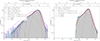 |
Fig. E.1. N-PDFs obtained from the various column density maps. Left: N-PDF of the high-res NH column density map derived using all Herschel dust data employing method I. Right: N-PDF of the NH column density map derived with method II. In solid red and dotted lines, the two-component log-normal fit is shown, whereas the power-law fits regimes are depicted in black dotted lines. The green lines show the N-PDF of H I. Here, m refers to the slope of the error tail for low column density, while α denotes the slope of the power-law tail for higher column densities. η is defined by |

The H I PDF exhibits a sharp decrease in the PDF shape for both low and high column densities. At high column densities, we enter a regime in which atomic hydrogen transitions to the molecular phase, explaining the edge observed in the shape. At low column densities, the cutoff limit of values in the map leads to a steep decrease in the PDF. The noise level of this map is approximately 2 × 1020 cm−2, which may partially account for the bump in the PDF. Additionally, we speculate that H I self-absorption (HISA) could contribute to the dip in the NHI-PDF around 4 × 1020 cm−2. However, this cannot be verified with the current datasets.
We fit the N-PDFs from method I with a combination of two log-normal and a PLT in the low and high density regime, similar to Spilker et al. (2021) with:
where the visual extinction AV is related to the total hydrogen column density by NH = AV ⋅ 1.87 × 1021 cm−2 mag−1 (Bohlin et al. 1978). The coefficients a1 and a2 represent the normalisation factors of both log-normal distributions. x0 is the first transition point from the noise slope at low column density to the log-normal regime. x1 is the second transition point indicating the change from the log-normal regime to the power-law regime at high column density. Both transition points have been fitted as well. σ1, 2 are the widths of the first and second log-normal and μ1, 2 their respective peaks. Since the shape of the N-PDF obtained with method II does not allow us to utilise the model given in Eq. E.1, we skip the first part of Eq. E.1 for values below the first transition x0 and start with a log-normal instead.
Figure E.1 displays the results of the fitting process. The solid red line represents the entire fit, while the dashed red lines represent the log-normals. The peaks and widths of these log-normals are presented in the small panel, along with the slope α of the high-density PLT that was fitted. The slope m characterises the low-density error tail and has a value of 1.1 for method I. It is worth noting that the fit for method II is purely formal due to the absence of a portion of the noise. A value of around 1 for the noise slope, as per Ossenkopf-Okada et al. (2016), suggests that low column densities are primarily influenced by noise. When the noise level decreases, the slope increases. In any case, noise contributes to the broadening of the N-PDF, resulting in a width of σ = 0.4 for the first log-normal for both methods. The peak of the first log-normal is 2 × 1020 cm−2 for method I and 6 × 1020 cm−2 for method II. This finding is roughly consistent with the excess in the gas distribution observed in the inter-main spiral and outer regions of M33, as depicted in Fig. 4 (left). The first peak of the NH-PDF of method I approximately corresponds to the first peak of the NHI-PDF, while for method II, the NH-PDF is found at higher column densities and corresponds more to the dip in the NHI-PDF. However, it is important to note that the fit of the N-PDF for method II presents challenges due to the inadequate description of the low column density range, resulting in an excess at the intersection of the error slope and the first log-normal. Another caveat of method II is the difficulty in distinguishing the transition of the first log-normal fit to the PLT tail. Due to the relatively high peak at 6 × 1020 cm−2 and the large width of σ = 0.4, the transition between both can potentially occur over a wide range, leading to increased uncertainty in determining the slope of the PLT in method II.
The peaks of the second log-normal exhibit the same value of 1 × 1021 cm−2 and a width of σ = 0.3 and σ = 0.2 for methods I and II, respectively. Interpreting the N-PDFs of extragalactic data is different from Galactic data. In the Galactic context, the correlation between the peaks in H I and the total hydrogen PDF in principle suggest that the first log-normal in the N-PDF predominantly comprises atomic gas. Conversely, the second log-normal would likely originate from molecular gas. This behaviour has previously been observed in a diffuse cloud in the Milky Way (Schneider et al. 2022). However, as mentioned in Sect. 4.1, it is essential to compare corresponding regions of the maps. Thus, the excess in the total N-PDF (see Fig. E.1) at higher column densities surpassing the highest values of the NH I-PDF can be attributed to molecular gas, similar to the approach used in Fig. 5.
As at high column densities, gravitational collapse of entire GMC or clumps within them, expect to form PLTs, we tentatively conduct a fitting procedure to determine the slope at the high column density regime, obtaining values of α = −1.8 and α = −2.6 for methods I and II, respectively. These values align with expectations for the gravitational collapse of an isothermal spherical density distribution, as described by Larson (1969) and Whitworth & Summers (1985). We note, however, that these findings are very preliminary and more data with higher resolution and a broader dynamic range are essential to provide a robust justification for these results.
Appendix F: The radial profile of the XCO factor
The radial profile of the XCO factor is given in Fig. F.1 and shows a relatively flat dependency for both XCO maps. Each data point corresponds to a bin of 100 pc. The mean value has been calculated for each bin, and the colour indicates the standard deviation of the bin. The error bars represent the standard error  , where σ denotes the standard deviation and N the samples number. Only one error bar is displayed for each method, as the overall error bars remain relatively similar, hence being representative, and including all of them might distract from the focus on the radial profile. While the overall uncertainty is already substantial when taking all data into account, it increases further as fewer data points are utilised per 100 pc bin, demonstrating a substantial spread in the values within each bin. A visual inspection of Fig. 7 suggests an increase in the XCO factor towards the centre, which is also indicated by a quantitative analysis of the radial profile revealing a slight decrease relative to values at ∼ 2 kpc and being flat until ∼ 4 kpc. Beyond ∼ 4 kpc the profile separates between the two methods. Method I shows a decrease, while method II shows an increase. However, the scatter beyond ∼ 4 kpc becomes even larger due to fewer data points, which corresponds to the extent of the main spiral arms (see Fig. 7).
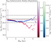 |
Fig. F.1. Radial profile of the XCO factor as a function of the galactocentric radius in bins of 100 pc. Reddish data points refer to the XCO factor obtained with method I, while the green to bluish represent XCO obtained with method II. The uncertainty of each bin is given by the colour scale and the error bars represent the standard error ( |

F.1. Discussion of the radial profile
In a study by Sandstrom et al. (2013), the radial profile of the XCO conversion factor has been examined in a sample of 26 nearby galaxies, excluding M33. Their analysis revealed that many galaxies exhibit a decreased XCO factor by a factor of approximately 2 towards the centre, while maintaining a consistently flat dependency on the galactocentric radius. Some galaxies show no decrease towards the centre, but rather a slight increase, which we see in M33 as well.
Despite the large scatter of XCO across the galactocentric radius (as shown in Fig. F.1), it is tentatively inferred that the radial dependence of XCO in M33 is also flat, which is consistent with the conclusions drawn by Sandstrom et al. (2013). The low correlation coefficients of approximately −0.3 for both Spearman and Pearson correlation coefficients indicate a weak correlation, thus providing further support for this conclusion. In our data, obtained using method I, there is an increase beyond ∼ 4 kpc, while for the data obtained via method II, there is a decrease. Both trends coincide with an increase in uncertainty due to fewer data points beyond ∼ 4 kpc (see Fig. 7). Considering the large uncertainty, the radial trend still remains relatively flat.
However, the decline with galactocentric radius could be due to CO turning optically thin in the outskirts of the galaxy but given the high uncertainty from the few data points and a drop of merely ∼ 20% this is not significant. It will certainly not affect any global properties in M33 so that we consider the radial profile of the XCO factor rather as predominantly flat. The absence of a pronounced decrease towards the centre might be attributed to an augmented optical depth of the CO emission, as previously mentioned. The used line ratio of 0.8 is only an average and may bias the radial profile we observe, as it varies across the disk of M33 (Druard et al. 2014). However, there is no radial trend in the variation of this ratio, cancelling out rather large-scale effects along the galactocentric radius. Also of crucial importance is the disparity in critical density between CO(1 − 0) and CO(2 − 1), implying possible variations in the extent of the clouds (as previously mentioned). However, this effect is potentially mitigated by smoothing the CO data to reduce it to a lower resolution.
All Tables
Parameters used to calculate column or surface densities of molecular hydrogen in several studies of M33.
All Figures
|
Fig. 1. NH I and CO line-integrated intensity map. Left: H I column density map determined from VLA H I observations (Gratier et al. 2010). Right: IRAM 30 m CO(2 − 1) line integrated intensity map of M33 (Druard et al. 2014). The lines in the colour bar mark the 3σ and 6σ values of CO emission. Both maps are smoothed to a resolution of 18.2″ and re-gridded to a pixel size of 6″. CO contours at 3 and 6σ are overlaid on both maps. |
| In the text | |
|
Fig. 2. κ0 map obtained as described in Sect. 3.2. Note that the DGR is included in the notation of κ0. CO contours at the 2σ level are overlaid on the map. |
| In the text | |
|
Fig. 3. Total hydrogen column density maps obtained via methods I and II. Left: high resolution NH total gas column density map obtained from the Herschel maps of M33 at 18.2″ angular resolution using the β map from Tabatabaei et al. (2014) with method I. Right: total gas column density map NH obtained from the Herschel SPIRE 250 μm map of M33 with method II at the same spatial resolution of 18.2″, indicated by the circle in the lower left corner. CO contours (as of Fig. 1) are overlaid in both maps. The white dashed ellipses mark roughly the regions we refer to as ‘inter-main spiral’ region or “outskirts”. |
| In the text | |
|
Fig. 4. Molecular hydrogen column density maps obtained via methods I and II. Left: high-res H2 column density map derived using all Herschel dust data employing method I with CO contours above the 3 and 6 σ level of the CO map shown in Fig. 1. Right: H2 column density map derived from SPIRE 250 μm map with method II. The circle to the lower left represents the resolution of 18.2″. |
| In the text | |
|
Fig. 5. N-PDFs obtained from the various column density maps. Left: N-PDF of the high-res NH column density map derived using all Herschel dust data employing method I only for non-blanked pixels of Fig. 4. Right: N-PDF of the NH column density map derived with method II for the same non-blanked pixels of Fig. 4. The green lines show the N-PDF of H I. Here, η is defined by |
| In the text | |
|
Fig. 6. (NH, Method I − NH, Method II)/NH, Method II difference map of the dust-derived total column density maps. The grey ellipse roughly delineates the area of enhanced emission observed in the western half of M33, as depicted in Figs. 3 (left) and 4 (left), in contrast to the eastern half. |
| In the text | |
|
Fig. 7. XCO factor (ratio) maps of methods I and II. Determined as the dust-derived H2 column density over CO intensity determined at each position in both maps of M33 at 18.2″ and scaled with the |
| In the text | |
|
Fig. 8. Distribution of the XCO conversion factor from methods I and II in blue and green, respectively. The XCO(1 − 0) conversion factors of Fig. 7 and their standard deviations are given in the panel. A log-normal Gaussian fit is shown in the corresponding colours for methods I and II. |
| In the text | |
|
Fig. 9. Scatter plots of the dust-derived column density and CO(1 − 0) intensity determined for both maps of M33 at 18.2″. Grey data points correspond to those excluded in the fit. Top: scatter plot of method I. Bottom: scatter plot of method II. The estimated error of each individual data point is conservatively estimated to be 30%. |
| In the text | |
|
Fig. A.1. Herschel flux maps in MJy sr−1 at the four observing wavelengths with overlaid CO contours at 3σ, 6σ, and 12σ. |
| In the text | |
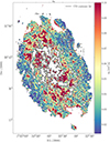 |
Fig. B.1. κ0 map obtained as described in Sect. 3.2 before filling holes with KNNImputer. |
| In the text | |
|
Fig. B.2. Emissivity index β map from Tabatabaei et al. (2014). CO contours at the 2σ level are overlaid on the map. |
| In the text | |
|
Fig. B.3. Temperature map obtained by Tabatabaei et al. (2014) used in both methods and in the determination of κ0. |
| In the text | |
|
Fig. C.1. Temperature maps obtained and used within both methods. Left: Temperature map at 500 μm obtained with method I. Middle: Temperature map at 350 μm obtained with method I. Right: Colour temperature map at 250 μm obtained with method I using the flux ratio of SPIRE 250 μm and PACS 160 μm. Note, this map was not used. |
| In the text | |
|
Fig. D.1. β map obtained by Tabatabaei et al. (2014) around NGC604 including areas of atomic and molecular phases. The contour lines represent the differences between our additional fit and the one of Tabatabaei et al. (2014), with values of −0.1, 0, 0.1 and 0.2 shown in white, red, blue and grey, respectively. |
| In the text | |
|
Fig. E.1. N-PDFs obtained from the various column density maps. Left: N-PDF of the high-res NH column density map derived using all Herschel dust data employing method I. Right: N-PDF of the NH column density map derived with method II. In solid red and dotted lines, the two-component log-normal fit is shown, whereas the power-law fits regimes are depicted in black dotted lines. The green lines show the N-PDF of H I. Here, m refers to the slope of the error tail for low column density, while α denotes the slope of the power-law tail for higher column densities. η is defined by |
| In the text | |
|
Fig. F.1. Radial profile of the XCO factor as a function of the galactocentric radius in bins of 100 pc. Reddish data points refer to the XCO factor obtained with method I, while the green to bluish represent XCO obtained with method II. The uncertainty of each bin is given by the colour scale and the error bars represent the standard error ( |
| In the text | |
Current usage metrics show cumulative count of Article Views (full-text article views including HTML views, PDF and ePub downloads, according to the available data) and Abstracts Views on Vision4Press platform.
Data correspond to usage on the plateform after 2015. The current usage metrics is available 48-96 hours after online publication and is updated daily on week days.
Initial download of the metrics may take a while.