| Issue |
A&A
Volume 693, January 2025
|
|
|---|---|---|
| Article Number | A88 | |
| Number of page(s) | 19 | |
| Section | Extragalactic astronomy | |
| DOI | https://doi.org/10.1051/0004-6361/202449738 | |
| Published online | 06 January 2025 | |
Interpreting millimeter emission from IMEGIN galaxies NGC 2146 and NGC 2976
1
Institute for Research in Fundamental Sciences (IPM), School of Astronomy, Tehran, Iran
2
Institut d’Astrophysique de Paris, Sorbonne Université, CNRS (UMR7095), 98 bis Boulevard Arago, 75014 Paris, France
3
Université Côte d’Azur, Observatoire de la Côte d’Azur, CNRS, Laboratoire Lagrange, France
4
School of Physics and Astronomy, Cardiff University, Queen’s Buildings, The Parade, Cardiff CF24 3AA, UK
5
Université Paris-Saclay, Université Paris Cité, CEA, CNRS, AIM, 91191 Gif-sur-Yvette, France
6
Université Grenoble Alpes, CNRS, Grenoble INP, LPSC-IN2P3, 38000 Grenoble, France
7
Max Planck Institute for Extraterrestrial Physics, Giessenbach-strasse 1, 85748 Garching, Germany
8
University of Ghent, Department of Physics and Astronomy, Ghent, Belgium
9
Aix Marseille Univ., CNRS, CNES, LAM (Laboratoire d’Astrophysique de Marseille), Marseille, France
10
Université Grenoble Alpes, CNRS, Institut, Néel, France
11
Institut de RadioAstronomie Millimétrique (IRAM), Grenoble, France
12
Dipartimento di Fisica, Sapienza Università di Roma, Piazzale Aldo Moro 5, I-00185 Roma, Italy
13
Univ. Grenoble Alpes, CNRS, IPAG, 38000 Grenoble, France
14
Centro de Astrobiología (CSIC-INTA), Torrejón de Ardoz, 28850 Madrid, Spain
15
Institut d’Astrophysique Spatiale (IAS), CNRS, Université Paris Sud, Orsay, France
16
IRAP, Université de Toulouse, CNRS, UPS, IRAP, Toulouse Cedex 4, France
17
National Observatory of Athens, Institute for Astronomy, Astrophysics, Space Applications and Remote Sensing, Ioannou Metaxa and Vasileos Pavlou, GR-15236 Athens, Greece
18
Department of Astrophysics, Astronomy & Mechanics, Faculty of Physics, University of Athens, Panepistimiopolis, GR-15784 Zografos, Athens, Greece
19
High Energy Physics Division, Argonne National Laboratory, 9700 South Cass Avenue, Lemont, IL 60439, USA
20
Instituto de Radioastronomía Milimétrica (IRAM), Granada, Spain
21
LERMA, Observatoire de Paris, PSL Research Univ., CNRS, Sorbonne Univ., UPMC, 75014 Paris, France
22
School of Earth and Space Exploration and Department of Physics, Arizona State University, Tempe, AZ 85287, USA
23
STAR Institute, Université de Liège, Quartier Agora, Allée du Six Aout 19c, B-4000 Liege, Belgium
24
Sterrenkundig Observatorium Universiteit Gent, Krijgslaan 281 S9, B-9000 Gent, Belgium
25
School of Physics and Astronomy, University of Leeds, Leeds LS2 9JT, UK
26
Laboratoire de Physique de l’École Normale Supérieure, ENS, PSL Research University, CNRS, Sorbonne Université, Université de Paris, 75005 Paris, France
27
Department of Physics and Astronomy, University of Pennsylvania, 209 South 33rd Street, Philadelphia, PA 19104, USA
28
University of Lyon, UCB Lyon 1, CNRS/IN2P3, IP2I, 69622 Villeurbanne, France
29
Dipartimento di Fisica, Università di Roma ‘Tor Vergata’, Via della Ricerca Scientifica 1, I-00133 Roma, Italy
⋆ Corresponding author; This email address is being protected from spambots. You need JavaScript enabled to view it.
Received:
26
February
2024
Accepted:
10
October
2024
Abstract
The millimeter continuum emission from galaxies provides important information about cold dust, its distribution, its heating, and its role in the interstellar medium (ISM). This emission also carries an unknown portion of the free-free and synchrotron radiation. The IRAM 30 m Guaranteed Time Large Project, Interpreting Millimeter Emission of Galaxies with IRAM and NIKA2 (IMEGIN) provides a unique opportunity to study the origin of the millimeter emission at angular resolutions of < 18″ in a sample of nearby galaxies. As a pilot study, we present millimeter observations of two IMEGIN galaxies, NGC 2146 (starburst) and NGC 2976 (peculiar dwarf) at 1.15 mm and 2 mm. Combined with the data taken with the Spitzer, Herschel, Planck, WSRT, and the 100 m Effelsberg telescopes, we modeled the infrared-to-radio Spectral Energy Distribution (SED) of these galaxies, both globally and at resolved scales, using a Bayesian approach to (1) dissect different components of the millimeter emission, (2) investigate the physical properties of dust, and (3) explore the correlations between millimeter emission, gas, and star formation rate (SFR). We find that cold dust is responsible for most of the 1.15 mm emission in both galaxies and at 2 mm in NGC 2976. The free-free emission emits more importantly in NGC 2146 at 2 mm. The cold dust emissivity index is flatter in the dwarf galaxy (β = 1.3 ± 0.1) compared to the starburst galaxy (β = 1.7 ± 0.1). Mapping the dust-to-gas ratio, we find that it changes between 0.004 and 0.01 with a mean of 0.006 ± 0.001 in the dwarf galaxy. In addition, there is no global balance between the formation and dissociation of H2 in this galaxy. We find tight correlations between the millimeter emission and both the SFR and molecular gas mass in both galaxies.
Key words: galaxies: dwarf / galaxies: ISM / galaxies: individual: NGC 2146 / galaxies: individual: NGC 2976 / galaxies: spiral / galaxies: starburst
© The Authors 2025
 Open Access article, published by EDP Sciences, under the terms of the Creative Commons Attribution License (https://creativecommons.org/licenses/by/4.0), which permits unrestricted use, distribution, and reproduction in any medium, provided the original work is properly cited.
This article is published in open access under the Subscribe to Open model. This email address is being protected from spambots. You need JavaScript enabled to view it. to support open access publication.
1. Introduction
Dust is one of the most important constituents of the interstellar medium (ISM) of galaxies, catalyzing the formation of molecules needed to form protostellar cores (Gould & Salpeter 1963; Perets & Biham 2006; Bron et al. 2014). By absorbing starlight and re-emitting it at infrared to millimeter wavelengths (λ ∼ 5 μm–3 mm), dust significantly impacts the heating and cooling processes of the ISM, and thus has a profound influence on the overall physics of a galaxy (Tielens 1997; Smith et al. 2007; Pope et al. 2008; Galametz et al. 2013; Nersesian et al. 2019) as well as its appearance in the ultraviolet to infrared wavelength range. Modeling the spectral energy distribution (SED) of dust allows us to infer the physical properties of the grains, such as their temperature, mass, composition, and size distribution. Understanding these properties and their relationship with other components of the ISM, such as gas and star formation tracers, is essential in order to understand the evolution of the galaxy (Draine et al. 2007; Galametz et al. 2009; Kramer et al. 2010; Aniano et al. 2012, 2020; Tabatabaei et al. 2014; Orellana et al. 2017; Galliano et al. 2018).
Dust in galaxies emits across a range of temperatures. The warmer more emissive component of dust emits mostly in the mid-infrared (MIR) wavelength range. In contrast, the colder and more massive dust component emits at longer wavelengths in the far-infrared (FIR), up to 3 mm. This cold (15−30 K) dust component is heated by the diffuse interstellar radiation field (ISRF), mainly fed by photons from the global stellar population. However, the emission from this cold component is often intermixed with emission from warmer dust peaking at λ ∼ 70 μm, which is heated by star-forming regions, and hence it is often poorly constrained. The submillimeter/millimeter waveband (500−3000 μm) is crucial for detecting this cold dust component, and thus for making accurate estimates of the total dust mass (Boquien et al. 2011; Tabatabaei et al. 2013a).
Space telescopes such as IRAS, ISO, Spitzer, and Herschel have allowed us to study dust emission in galaxies up to 500 μm. These telescopes have provided sensitive MIR to FIR observations to constrain the dust properties, particularly around the peak of the dust SED (100−200 μm in star-forming galaxies). However, studying longer millimeter wavelengths, well beyond the peak, is crucial for modeling the mass and temperature of cold dust (e.g., Galliano et al. 2003; Galametz et al. 2011; Rémy-Ruyer et al. 2013; Hunt et al. 2015). To fully sample the dust SED, reliable data in the millimeter range is needed. The Planck space telescope has observed the Milky Way and other galaxies at millimeter wavelengths, but its resolution (300″ at best) does not allow the study of resolved ISM in most galaxies. As a result, even for many nearby galaxies, we lack high-resolution observations at the low-frequency end of their dust SED. This coarse sampling of the Rayleigh-Jeans tail of dust emission in most galaxies has resulted in poor constraints on the content and physical properties of cold dust in those objects.
The New IRAM KID Array (NIKA2) on the IRAM 30 m telescope, with an instantaneous field of view (FoV) of 6.5′ and angular resolutions of 11.1″ and 17.6″ at 260 and 150 GHz, respectively, is an ideal instrument for studying the dusty ISM of nearby galaxies in detail (Adam et al. 2018; Perotto et al. 2020). The Guaranteed-Time Large Project of the NIKA2 collaboration, Interpreting Millimeter Emission of Galaxies with IRAM and NIKA2 (IMEGIN), led by S. Madden, has observed a sample of 22 nearby galaxies with varying ranges of masses, morphological types, star formation rates (SFRs), and ISM properties with distances less than 25 Mpc. This sample is expected to provide essential data for studying the thermal emission of cold dust and its relation to other components of the ISM in nearby galaxies. The first IMEGIN paper was focused on the edge-on galaxy NGC 891 (Katsioli et al. 2023). This paper is the second IMEGIN paper that presents and analyzes the NIKA2 observations of the two galaxies, NGC 2146 and NGC 2976. These two galaxies, which differ extensively in terms of mass, SFR, and ISM properties, were among the first IMEGIN galaxies to have their observations and data processing completed, which is the reason why we selected these galaxies for this paper.
NGC 2146 is a barred spiral galaxy with a morphology type of SB(s)ab pec (de Vaucouleurs et al. 1991) and a total stellar mass of log M* = 10.3 M⊙ (Kennicutt et al. 2011). In optical images it shows a bright central bulge and extended irregular arms, in addition to an apparent dust lane that runs along the major axis. NGC 2146 is a luminous infrared galaxy (LIRG) with L8−100 μm ∼ 1011 (Gao & Solomon 2004). As outflows are reported to be common in LIRGs, NGC 2146 shows a superwind outflow along the minor axis that is observed in optical and in X-ray (Greve et al. 2000; Kreckel et al. 2014). Moreover, Taramopoulos et al. (2001) claimed that NGC 2146 went through a merger with a gas-rich low surface brightness spiral companion that occurred about 1 Gyr ago. The companion was destroyed during the interaction, as there is no evidence of a double-nucleus in the center of the galaxy, indicating that it is a highly evolved merger (Tarchi et al. 2004). This merger is believed to be the cause of the starburst activity in NGC 2146, given the high SFR of this galaxy, reported to be as high as SFR = 39 ± 11 M⊙ yr−1 (Nersesian et al. 2019). The metallicity reported for NGC 2146 is 12 + log(O/H) = 8.78 ± 0.16 (De Vis et al. 2019, from the calibration of Pettini & Pagel 2004), equal to 1.2 Z⊙, where Z⊙ is the solar metallicity (Asplund et al. 2009). The properties of NGC 2146 are presented in Table 1.
Properties of NGC 2146 and NGC 2976.
NGC 2976 is a peculiar dwarf galaxy (type SAc pec, de Vaucouleurs et al. 1991), a weakly disturbed satellite member of the M 81 group. It is a pure disk object with no visible spiral arms, although it is debated whether it has a gas-rich bar and large-scale arms (Valenzuela et al. 2014). NGC 2976 has a mass 22 times lower than that of NGC 2146 and a SFR of 0.13 ± 0.02 M⊙ yr−1 (Nersesian et al. 2019). The reported metallicity for this galaxy is 12 + log(O/H) = 8.39 ± 0.03 (De Vis et al. 2019, from the calibration of Pilyugin & Grebel 2016), equal to 0.5 Z⊙. The properties of NGC 2976 are summarized in Table 1.
This paper is organized as follows. After explaining the NIKA2 observations and the complementary data in Sect. 2, we present the resulting millimeter maps in Sect. 3. We then describe the framework for modeling the SED of continuum emission from the radio to FIR domains, and present the results on both global and resolved scales in Sect. 5. Our results are then discussed in Sect. 6 and summarized in Sect. 7.
2. Data
2.1. NIKA2 observations
We observed NGC 2146 and NGC 2976 as a part of IMEGIN with NIKA2, which operates simultaneously at two wavelengths, 1.15 mm and 2 mm. Observations of NGC 2146 were conducted from 13 to 17 January 2021. A total of 46 scans were taken during 6.2 hours of on-the-source telescope time. The sky conditions were stable. In addition, the atmospheric opacity τ225 GHz ranged between 0.11 and 0.28, with an average of 0.23 ± 0.05. NGC 2976 was observed between 25 October 2020 and 14 February 2021. In total, 66 scans were taken in 8.3 hours of on-the-source telescope time. During this time, the sky opacity τ225 GHz varied in the range 0.19 and 0.32, on average equal to 0.22 ± 0.06.
In general, the scans were conducted along directions at ±45° relative to the major axis of each galaxy. The scan sizes were 17.3′×8.12′ and 17.6′×7.35′ for NGC 2146 and NGC 2976, respectively. The on-the-fly scans were conducted at the maximum possible scanning speed for both galaxies (60″/s), given the elevation of the source at the time of the observations and the limitations of the telescope drive system to overcome sky fluctuations as much as possible. Pointing was corrected every hour, and the focus was adjusted every three hours.
The NIKA2 data were reduced with the Scanam_nika pipeline, as explained in Appendix A. The reduced observed maps at 1.15 mm and 2 mm are presented in Fig. 1. The color bars show the flux density in units of mJy beam−1, and beam sizes are indicated as a filled circle in the lower left corner of each map. The 1.15 mm maps have an original resolution, full width at half maximum (FWHM), equal to 12″ and a pixel size of 3″. In Fig. 1, the beam of the 1.15 mm maps corresponds to a physical scale of ∼1 kpc and ∼0.2 kpc in NGC 2146 and NGC 2976, respectively. The original resolution of 2 mm maps, on the other hand, is 18″, which corresponds to ∼1.6 kpc and ∼0.3 kpc physical scale in NGC 2146 and NGC 2976, respectively (Table 1). The pixel size of 2 mm maps are also 3″. In addition, we were able to reach a 1σrms noise level of 0.98 mJy/beam at 1.15 mm and 0.47 mJy/beam at 2 mm for NGC 2146. Similarly for NGC 2976, a 1σrms noise level of the 1.15 mm map is 0.97 mJy/beam, while it is 0.37 mJy/beam at 2 mm.
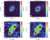 |
Fig. 1. Observed NIKA2 maps of NGC 2146 (top) and NGC 2976 (bottom) at 1.15 mm (left) and 2 mm (right). The color bars show the flux density in units of mJy/beam. The circle in the bottom left corner of each panel indicates the angular resolution (beam widths) which is 12″ and 18″ at 1.15 mm and 2 mm, respectively. The contours show the MIPS 24 μm emission at levels 9, 54, and 324 Jy/pixel in the top panels and 0.8, 2.4, and 7.2 Jy/pixel in the bottom panels. The FoV is 4′×4′ and 5′×5′ for NGC 2146 and NGC 2976, respectively. |
2.2. Complementary data
Table 2 summarizes the complementary data used in this work. A collection of the maps used in this work is presented in Figs. 2 and 3 for NGC 2146 and NGC 2976, respectively. We further explain the complementary data below.
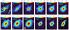 |
Fig. 2. Complementary data used in this work for NGC 2146. GALEX FUV, Spitzer MIPS, Herschel SPIRE and PACS, radio, and CO(2−1) maps are presented. The optical image in the Red filter displays the optical features of this galaxy and is not used in the analysis. The Planck 1.38 mm and radio 6.2 cm maps are also not shown due to poor resolution. All the demonstrated maps have the same FoV of 3.5′×4′, centered on the galaxy. The maps are displayed in logarithmic scale and their original resolution (see indicated Table 2); the beam size is represented by a white circle in the bottom left corner of each map. |
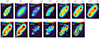 |
Fig. 3. Same as Fig. 2, but for NGC 2976. The HI map, which is only available for this galaxy, is also included. The optical map in the Red filter displays the optical features of this galaxy and is not used in the analysis. The Planck 1.38 mm and radio 6.2 cm maps are also not shown due to poor resolution. All the demonstrated maps have the same FoV of 3.7′×4.2′ centered on the galaxy. The maps are all shown in logarithmic scale and at their original resolution (see Table 2); the beam size is represented by a white circle in the bottom left corner of each map. |
Complementary data used in this study and their properties.
Both these galaxies were observed with Spitzer MIPS. NGC 2976 was observed as part of the Spitzer Nearby Galaxies Survey (SINGS, Kennicutt et al. 2003) project and NGC 2146 by Engelbracht et al. (2008). We acquired the MIPS 24 μm data from the DustPedia archive (Clark et al. 2018).
These galaxies were also observed with Herschel PACS and SPIRE cameras as part of the Key Insight in Nearby Galaxies: A Far-Infrared Survey (KINGFISH, Kennicutt et al. 2011) project. Moreover, we acquired Planck observations of these two galaxies at 1.38 mm from the DustPedia archive (Clark et al. 2018), originally presented in Planck Collaboration I (2014).
NGC 2146 and NGC 2976 were observed at 6 cm with the Effelsberg 100 m telescope as part of the Key Insight in Nearby Galaxies Emitting in Radio (KINGFISHER, Tabatabaei et al. 2017) project with 2.5′ angular resolution. Resolved radio continuum (RC) maps of these galaxies were taken with the Westerbork array as part of the WSRT SINGS project (Braun et al. 2007) with 10″ and 12.5″ angular resolutions at 18 cm and 21 cm wavelengths, respectively. In addition, we used archival photometry from Niklas et al. (1995), which includes observations at 2.8 cm with the Effelsberg 100 m telescope.
To take into account the contamination by the CO line emission in the NIKA2 1.15 mm observations and to trace molecular gas, we used CO(2−1) data from the HERA CO Line Extragalactic Survey (HERACLES, Leroy et al. 2009, 2013; Schruba et al. 2011; Sandstrom et al. 2013), observed with IRAM 30 m telescope. In order to study different neutral gas components, we made use of the VLA HI 21 cm observations as part of The HI Nearby Galaxy Survey (THINGS, Walter et al. 2008) project, which is available only for NGC 2976. As explained in Schruba et al. (2011), the HI emission from the disk of NGC 2146 is severely self-absorbed, which left us without useful information on the neutral atomic gas from millimeter-emitting regions of this galaxy.
We also used GALEX far-ultraviolet (FUV) data of these galaxies (Gil de Paz et al. 2007) acquired from the DustPedia archive (Clark et al. 2018). For the sake of comparison with optical structures, Figs. 2 and 3 also show R-band optical maps observed with the Jacobus Kapteyn Telescope (JKT, James et al. 2004). We note, however, that they were not used in this analysis.
3. Millimeter emission from NGC 2146 and NGC 2976
Figure 1 shows that the millimeter emission emerges from an elliptical disk that is brightest toward the galaxy center in NGC 2146. No characteristic galactic substructures, such as spiral arms, are evident at millimeter wavelengths, which is similar to what is found at FIR/submillimeter and radio wavelengths (Fig. 2). The maximum flux density is ≃95 mJy/beam at 1.15 mm and 55 mJy/beam at 2 mm at the position of the nucleus at the central source. The integrated flux densities are 529 ± 38 mJy and 130 ± 9 mJy at 1.15 mm and 2 mm, respectively.
NGC 2976, on the other hand, shows more structural details due to its proximity. Notably, the two bright star-forming regions in the north and south of this galaxy are prominent in the NIKA2 maps, similar to those in the FIR maps (Fig. 3). Its maximum occurs in the northwestern star-forming region with values of 14.0 mJy/beam and 6.2 mJy/beam at 1.15 mm and 2 mm, respectively. The southeastern source peaks at 10.8 mJy/beam at 1.15 mm and 4.4 mJy/beam at 2 mm. The integrated flux of the 1.15 mm and 2 mm maps are 465 ± 34 mJy and 84 ± 8 mJy.
The observed millimeter emission represents a mixture of thermal dust and free-free emission as well as the nonthermal synchrotron emission. In star-forming galaxies the free-free and synchrotron radiations are extinction-free tracers of the SFR (e.g., Condon 1992; Tabatabaei et al. 2017; Heesen et al. 2022). The radiation from dust grains is due to heating by different sources, and the peak of dust emission depends on the average energy of the radiation field. Warmer dust is heated mainly by the energetic radiation field near young massive stars dominated by UV photons, and therefore emit at shorter wavelengths. Colder dust, which emits at longer wavelengths, is heated mainly by the less energetic ISRF, dominated by optical photons from the old stellar population (see, e.g., Bendo et al. 2015). However, the ISRF itself depends on local physical conditions within a galaxy, such as the star formation rate and the ISM density of a galaxy. For instance, the ISRF in a starburst galaxy is expected to be dominated by ionizing UV photons from young massive stars rather than optical photons from old stars. There is a similar expectation in a dwarf star-forming galaxy with a low-density ISM, due to weak shielding and a high probability of the escape of ionizing photons. Despite different dust heating sources, the total IR emission of galaxies (e.g., integrated in the wavelength range of 8–1000 μm) is also widely used as a tracer of the SFR (Kennicutt & Evans 2012). On the other hand, cold dust emission can also trace the total gas content of galaxies, including dark gas, that is not traced by CO or HI (e.g., Abdo et al. 2010). Considering that the SFR and the gas surface densities are correlated through the Kennicutt–Schmidt relation, a more indirect correlation between the cold dust emission and the SFR is also expected (Boquien et al. 2011; Bendo et al. 2012). Hence, the millimeter emission can be strongly correlated with SFR and/or the molecular gas content of galaxies. Figure 1, which includes contours of 24 μm emission as a tracer of SFR overlaid on NIKA2 maps, shows a strong agreement between the two. This is further investigated in Sect. 6.1. We determined the contribution of each millimeter component through modeling the FIR-radio SEDs. This was also needed to study the physical properties of dust. Prior to the SED analyses, we assessed and subtracted the CO line contamination.
4. Contribution of the CO(2–1) emission
The NIKA2 passband at 1.15 mm overlaps partly with the CO(2−1) molecular line emission at 230.5 GHz (Perotto et al. 2020). Therefore, while measuring the continuum flux of our targets at 1.15 mm with NIKA2, we inevitably included line emission from CO(2−1). Hence, to study dust continuum emission separately, we had to determine the contamination by the CO(2−1) line and subtract it from the total emission at 1.15 mm. In Appendix B we explain how we took the emission of the CO(2−1) line into account.
We quantified the contribution of the CO line emission at 18″ resolution as this was our working resolution throughout the analysis. Therefore, we convolved the NIKA2 1.15 mm and CO(2−1) maps to 18″ resolution. Figure 4 shows the map of the fraction of the NIKA2 1.15 mm emission that is attributed to CO (2−1), calculated for pixels with values above the 3σrms level. Up to 30% of the observed 1.15 mm emission is due to CO line emission in the starburst galaxy NGC 2146. Moreover, in this galaxy, most of the CO line contamination occurs along the forward dusty arm of this galaxy (cf. R-band optical map in Fig. 2). In NGC 2976 the CO fraction is smaller with a maximum of only 10% (Fig. 4), consistent with the fact that dwarf galaxies have smaller reservoirs of molecular gas.
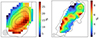 |
Fig. 4. Maps of the CO fraction defined as the ratio of the CO(2−1) line emission to the observed 1.15 mm emission in NGC 2146 (left) and NGC 2976 (right) at 18″ angular resolution. Only pixels above the 3σrms level of the observed NIKA2 map are shown. Contours show the intensity of CO emission in each galaxy, starting from 1σrms and increasing by factors of 3. The circles in the bottom left corners indicate the beam area. |
We found a mean CO(2−1) fraction (within pixels above 3σrms limit) of 17 ± 6% (error is the standard deviation) in NGC 1246 and 5 ± 2% for NGC 2976. We also derived a global value for the CO fraction by dividing the integrated fluxes of the CO(2−1) and NIKA2 1.15 mm maps (limited to above 3σrms levels). The global CO fraction amounts to 20% in NGC 2146, and lower (5%) in the dwarf galaxy NGC 2976.
5. SED modeling
As mentioned in Sect. 3, the emission at millimeter wavelengths is a combination of dust emission and the RC emission components: the thermal free-free and the nonthermal synchrotron emission. The observed continuum flux density at millimeter frequency ν ( ) can be expressed as
 (1)
(1)
where  is the thermal emission from dust, and
  is the total flux of the RC emission with
  being the thermal free-free emission and
  the nonthermal synchrotron emission. The synchrotron component has a power-law spectrum,
  , with αn the synchrotron spectral index and Asyn a scaling factor. The free-free emission is linearly proportional to the free-free Gaunt factor, gff(ν), assuming optically thin emission (Draine 2011). We model it as
  , where Aff is a scaling coefficient that depends weakly on the electron temperature Te1. It is often useful to report the fraction of the free-free emission in the RC component at a given frequency ν0, defined as
 (2)
(2)
Although the dust emission in the IR to millimeter range can represent a continuum of temperatures, we model the dust emission assuming a double-component modified blackbody (MBB) radiation, one from a warm dust component and the other from a cold dust component:
 (3)
(3)
Here M, T, and β are dust mass, temperature, and emissivity index, respectively, and Bν(T) is the Planck function. The suffixes c and w denote the cold and warm dust components. For the dust absorption coefficient, we use the value of κ0(200 μm) = 0.66 m2 kg−1 following Ysard et al. (2024).
In summary, we use the following equation to model the continuum emission in millimeter wavelengths:
 (4)
(4)
Equation (4) includes nine free parameters: Mc, Tc, βc, Mw, Tw, βw, Aff, Asyn, and αn. To reduce the number of free parameters and considering that warm dust constitutes only a small fraction of the total dust content of galaxies, we set βw = 2 throughout this work (Tabatabaei et al. 2014).
5.1. Global SED modeling
The SED model presented in Sect. 5 is used to fit the observed integrated flux densities from the IR to the radio wavelengths. This is required for a precise decomposition of the millimeter emission components and to obtain the global properties of dust in NGC 2146 and NGC 2976.
5.1.1. Photometry
We fit our SED model (Eq. 4) to the integrated flux densities at 24 μm, 70 μm, 100 μm, 160 μm, 250 μm, 350 μm, and 500 μm, as well as the millimeter and centimeter domain including NIKA2 1.15 mm and 2 mm, Planck 1.38 mm, RC 2.8 cm, 6.2 cm, 18 cm, and 21 cm. We obtained the integrated fluxes using the CASA software (CASA Team 2022). We integrated the maps in a circular aperture, using the task imstat in CASA. The radius of the reference circular aperture used for the photometry is 160″ and 175″ for NGC 2146 and NGC 2976, respectively, which is almost equal to R25 of each galaxy.
The resulting photometry values are listed in Table 3. The uncertainty of integrated fluxes in this table is computed following the method in Appendix C. Additionally, the integrated fluxes reported for NIKA2 1.15 mm and Planck 1.38 mm are corrected for the CO contamination, as explained in Sect. 4 and Appendix B.
Integrated flux densities of the maps used for the global SED analysis.
5.1.2. Fitting method and results
We employed a Bayesian approach to model the IR to radio SEDs on a global scale, utilizing all available maps in this range. We used the Markov chain Monte Carlo (MCMC) method to implement the Bayesian approach. For each free parameter, we reported the median of the posterior probability distribution functions as the resulting value and 20%–80% percentiles as error margins. During the fitting process, we accounted for the transmission functions of the various telescopes from which we obtained the data. The details of the fitting process are explained in Appendix D.
The SEDs modeled are illustrated in Fig. 5, including the uncertainty of the modeled flux as a shaded area. The relative residual (observation-model/observation) of each data point is shown in the bottom panels of each SED in Fig. 5. The relative residuals are 0% and 4% at 1.15 mm and 2 mm, respectively, in NGC 2146. For NGC 2976, they are 4% and 6% at 1.15 mm and 2 mm, respectively. At other wavelengths, the relative residuals are less than 10% (20%) in NGC 2146 (NGC 2976).
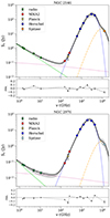 |
Fig. 5. Global IR-to-radio SED (solid black curve) and its decomposed individual components of the cold dust (blue dashed curve), warm dust (orange dot-dashed curve), free-free (purple dotted curve), and synchrotron emission (green solid curve) in NGC 2146 (top) and NGC 2976 (bottom). The shaded gray area shows the uncertainty of the model. The relative residual of the model and observations with respect to the observation is shown at the bottom of each plot. The resulting SED parameters are listed in Table 4. |
The resulting parameters listed in Table 4 show that a large part of the dust content in NGC 2146 has a temperature of ≃32 K, while only about 0.1% of it can be attributed to the warm dust component with a temperature of ≃88 K. A similar condition is present in NGC 2976, although most of the dust content is slightly colder (≃27 K) than that in NGC 2146. The total dust mass listed in Table 4 is consistent with previous findings reported by Hunt et al. (2019) and Nersesian et al. (2019) for both of these galaxies. Galliano et al. (2021) accounted for the mixing of the physical conditions in their dust modeling and obtained a higher dust mass (by a factor of 2). This disparity, as explained in Galliano et al. (2021), arises from the fact that the MBB model is an isothermal approximation and does not consider the coldest, less emissive, yet substantial regions in the galaxy, leading to a potential systematic underestimation of mass.
Resulting SED parameters in the global modeling.
Considering the RC components, we find a free-free fraction of  at 6 cm and
  at 21 cm for NGC 2146. Higher fractions are obtained for NGC 2976 with fff equal to
  and
and  at 6 cm and 21 cm, respectively, as expected for dwarf galaxies (Tabatabaei et al. 2017). Figure 5 shows that in NGC 2146 the free-free emission is dominating the SED between 25 and 240 GHz. The contribution of the free-free emission to total emission peaks at 67% at 76 GHz. Similar values have been reported in other starburst galaxies such as M 82 (Condon 1992; Peel et al. 2011) and NGC 3256 (Michiyama et al. 2020), or in the central starburst regions of normal star-forming galaxies such as NGC 4945 (Bendo et al. 2016), NGC 253 (Peel et al. 2011; Bendo et al. 2015), and NGC 1808 (Salak et al. 2017; Chen et al. 2023).
The global continuum emission of these two galaxies is decomposed into its three components at NIKA2 wavelengths: the emission from the free-free, synchrotron, and dust (Eq. 4). The results of this decomposition are reported in Table 5. As expected, moving from 1.15 mm to 2 mm, the contribution of dust emission decreases, while the contributions of free-free and synchrotron emission increase.
Contribution of the three constituents of continuum emission with respect to the modeled flux at 1.15 mm and 2 mm.
We note that at 2 mm, 87.3% of the emission is due to dust in NGC 2976, which agrees with that reported by Katsioli et al. (2023) for the normal star-forming galaxy NGC 891. However, this contribution is smaller in NGC 2146 (47.6%), indicating that this starburst galaxy has stronger radio emission at 2 mm. Therefore, we emphasize that assuming a dominant dust component at 2 mm is not always correct, and it can depend on the ISM and star formation properties.
5.2. Resolved SED modeling
In the following we describe the pixel-wise analysis of the IR-to-radio SED used to map the millimeter emission constituents (dust, free-free, and synchrotron), dust physical parameters, and the free-free fraction in NGC 2146 and NGC 2976.
5.2.1. Photometry
We chose 18″ (the FWHM at 2 mm and 250 μm) as our working resolution to study the SED on spatial scales of ∼1.6 kpc and ∼0.3 kpc in NGC 2146 and NGC 2976, respectively. Therefore, the Planck 1.38 mm, SPIRE 350 μm, SPIRE 500 μm, radio 2.8 cm, and radio 6 cm maps are excluded from this analysis due to their poorer angular resolutions (Table 2). We convolve the Spitzer MIPS, Herschel PACS and 1.15 mm map to the 18″ resolution using Gaussian kernels. The various bands sampling the dust SED were observed with different instruments, from space or on the ground, with very different final performance levels regarding flux conservation and noise subtraction. To homogenize the spatially resolved dust SED (both in terms of recovered flux fraction and noise properties), and in order to obtain reliable parameters from the SED fitting that are as unbiased as possible, we built simulations as explained in Appendix A.
The radio maps are similarly convolved with a Gaussian kernel with CASA software, using the task imsmooth. Ultimately, we reprojected all the maps to the same geometry and coordinate system and regridded them to 6″ pixel size. We note that the pixel size was chosen to be one-third of the beam size to ensure Nyquist sampling. Our analysis is limited to pixels with a signal-to-noise ratio, S/N > 3, for all maps used over the entire analysis.
5.2.2. Fitting method and results
The lack of resolved RC maps at 2.8 and 6 cm prevents us from constraining the synchrotron spectral index if it is chosen as a variable. Therefore, we opted to use the globally obtained αn (Table 4) for different pixels. We should note that this assumption is not entirely realistic because studies show that αn can vary in different parts of a galaxy (e.g., Tabatabaei et al. 2013b; Baes et al. 2010). However, to constrain the SEDs locally, more resolved maps are needed to cover the radio domain, which is not available currently. Moreover, to reduce parameter distribution biases caused by degeneracy and noise-injected correlations between the dust SED parameters, particularly that of the dust temperature and emissivity index (e.g., Shetty et al. 2009; Juvela & Ysard 2012; Kelly et al. 2012), we also fixed βc to its global value (see Table 4). This choice was then assessed by repeating the analysis using different fixed βc values around its global value in each galaxy (Table 6). The goodness of the SED fits was then evaluated for each βc selected. In the context of the Bayesian approach, posterior predictive p-values are used to assess the quality of a fit (Galliano et al. 2021; Galliano 2022). In this method, a p-value close to 0.5 suggests that the model is a good fit for the data, while a p-value close to 0 or 1 suggests that the model may not be a good fit. The p-values per pixel for each βc are calculated and reported in Table 6. The data is best reproduced taking βc = 1.8 for NGC 2146 and βc = 1.4 for NGC 2976, which agree with the global results (Table 4) taking into account their uncertainties. We note that fixing βc is a first approximation, as it can spatially vary inside a galaxy (Tabatabaei et al. 2014).
Mean of p-values in the pixel-wise SED modeling with a fixed βc.
For the resolved study, Eq. (4) is applied using the flux densities per pixel instead of the integrated flux densities. Similarly to the global study, we implemented the MCMC Bayesian inference. The fitting method and uncertainties are explained in detail in Appendices C and D. Figure 6 shows the resulting SEDs of a selected pixel for each galaxy. The resulting parameter maps (i.e., medians of the posterior distribution functions) for Tc, ΣMc, Tw, ΣMw, and fff(21 cm), along with their relative uncertainty maps, are shown in Figs. 7 and 8. We note that the surface density of the dust mass is corrected for the inclination of each galaxy. The mean value and dispersion of each parameter are reported in Table 7. These maps are discussed as follows.
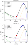 |
Fig. 6. IR-to-radio SEDs of a selected pixel in NGC 2146 (top) and NGC 2976 (bottom). The curves show the cold dust (blue dashed curve), warm dust (orange dot-dashed curve), free-free (purple dotted curve), and synchrotron (green solid curve) emissions. |
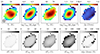 |
Fig. 7. Maps of the resulting SED parameters for NGC 2146 for 6″ pixels (≃525 pc). Shown (from left to right) are cold dust temperature Tc (K), cold dust mass surface density |


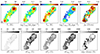 |
Fig. 8. Same as Fig. 7, but for NGC 2976. The SED analysis only uses pixels with intensities > 1σrms at all wavelengths for this dwarf galaxy. |
Statistics of resolved SED modeling.
In NGC 2146, no spiral arms or star-forming regions are evident in the resulting SED parameter maps at the resolution of this study (∼1.6 kpc), as expected from the observed maps (Fig. 1). With Tc varying mainly in a narrow range of  to
to  K, the cold dust component has a higher surface density in the inner disk of NGC 2146 reaching a maximum of
  in the center of this galaxy. The warm dust component (
 K) becomes denser toward the center reaching a peak of
  . The mass surface density of the warm dust is lower than that of the cold dust by more than two orders of magnitude while its variation over the galaxy is three times larger. Both Tc and Tw are higher in the inner part of this galaxy, with slightly different distributions, but overall consistent within the error margins.
At about 0.3 kpc resolution, the resulting SED parameter maps exhibit resolved structures in NGC 2976. Cold dust with temperatures ranging between  K and
K and  K is denser in the star-forming regions, particularly the one in the northwest that hosts the maximum surface density of
  . The warm component with temperatures ranging between
  K and
K and  K follows a similar distribution, although it is more concentrated in the star-forming regions compared to the cold dust (the star-forming versus non-star-forming contrast is five times larger than that of the cold dust). The cold and warm components have similar temperature distributions across NGC 2976, although Tw has a higher fluctuation than Tc. This indicates that both components are effectively heated by young massive stars in this galaxy.
Figures 7 and 8 also present the maps of the free-free fraction, fff (Eq. 2), at 21 cm. We note that the large relative errors δfff are due to poor sampling of the SED in the radio domain, particularly in regions of lower S/N. In NGC 2146, fff varies between 10% in the outskirts and 20% in the inner disk of this galaxy, but with δfff as large as 50%. The mean fff obtained is the same as the global value reported in Sect. 5.1 and agrees with that of spiral galaxies (Tabatabaei et al. 2017). In NGC 2976, about 100% of the RC emission is due to the free-free emission in its star-forming regions in the north and south, with a small relative error. In other regions, fff is about 50%, but largely uncertain. This is also consistent with the global analysis showing that the free-free emission has an important contribution to the observed RC emission from this dwarf galaxy.
The contributions of different components of the millimeter emission at 1.15 mm and 2 mm are shown in Fig. 9. The mean of each map is consistent with its globally determined contribution listed in Table 5. Several known facts are demonstrated in this figure; for example, moving from 1.15 mm to 2 mm, the contribution of dust emission decreases, while that of the RC emission increases, as expected from the model. In addition, Fig. 9 shows that in both galaxies and at both millimeter wavelengths, the RC emission is dominated by the free-free emission. In NGC 2976, the 1.15 mm emission is almost entirely produced by dust, but at 2 mm, the free-free emission becomes as strong as dust emission in the star-forming regions, resulting in equal contributions. This trend is more pronounced in NGC 2146, where the contribution of the free-free emission increases more than that of dust in the inner disk, moving from 1.15 mm to 2 mm. In addition, synchrotron emission is negligible at both wavelengths in NGC 2976, whereas it has a contribution as large as 30% at 2 mm in NGC 2146. We note that a larger contribution of dust emission in NGC 2976 does not mean that a larger amount of dust is present in the ISM of this dwarf galaxy; it simply shows that NGC 2146 emits the free-free and synchrotron radiation much more intensely than NGC 2976 at millimeter wavelengths. This is clearly seen in Figs. 2 and 3 and Tables 4 and 7. Consequently, we emphasize that dust may account for only 30% of the observed 2 mm emission in certain regions of a starburst galaxy.
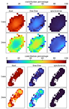 |
Fig. 9. Contribution percentage from dust (left column), free-free (middle column), and synchrotron (right column) emission in the total modeled flux at 1.15 mm (top row) and 2 mm (bottom row) are shown for NGC 2146 (top panel) and NGC 2976 (bottom panel). |
Finally, subtracting the contributions of the free-free and synchrotron emission from the observed millimeter emission, we present maps of the pure dust emission (the sum of both warm and cold dust emission) at 1.15 mm in Fig. 10 (see Eq. 3). We recall that the 1.15 mm emission was already corrected for the contamination by the CO(2−1) line emission in Sect. 4.
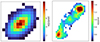 |
Fig. 10. Map of pure dust emission at 1.15 mm (after subtraction of the CO line contamination, free-free, and synchrotron emission) in mJy/pixel in NGC 2146 (top) and NGC 2976 (bottom). |
6. Discussion
In the previous sections we show that the NIKA2 observations enable the IR-to-radio SED of galaxies in the millimeter domain to be constrained. We determined the contribution of dust emission to millimeter emission at 18″ angular resolution and presented maps of the mass and temperature of the cold and warm dust components in NGC 2976 and NGC 2146. In this section we explore any correlations between the NIKA2 maps and the SFR and molecular gas tracers in NGC 2146 and NGC 2976 as prototypes for starburst and dwarf galaxies, respectively. Then, we discuss the interplay between dust and total neutral gas in NGC 2976.
6.1. Relating millimeter emission to SFR and molecular gas
As discussed in Sect. 3, the millimeter continuum emission can be strongly correlated with the SFR and with the molecular gas. The correlation with SFR is indicated by an agreement between the millimeter emission and the 24 μm emission contours in both NGC 2146 and NGC 2976 in Fig. 1. We further investigate the correlations between the 1.15 mm and 2 mm emission observed with NIKA2 and the surface density of SFR (ΣSFR) as well as the molecular gas surface density (ΣH2) in more detail.
To compute ΣSFR, we used the dust emission at 24 μm (assuming heating by young massive stars as its main source) in combination with dust-obscured FUV emission as a hybrid SFR tracer. The calibration proposed by Hao et al. (2011) combines Spitzer MIPS 24 μm observations with GALEX FUV observations to compute the SFR with the following relation: SFR = 3.36 × 10−44(LFUV + 3.89L24 μm). In this relation, the SFR is expressed in M⊙ yr−1 and luminosity in erg s−1, and a Kroupa IMF (Kroupa & Weidner 2003) is assumed. We additionally corrected for the inclination of each galaxy.
To compute the molecular hydrogen gas mass, we used CO(2−1) line emission as a tracer. We used the relation given in Leroy et al. (2009), which is ![Mathematical equation: $ \Sigma_{\mathrm{H}_2}\,[\mathrm{M}_{\odot}\,\mathrm{pc}^{-2}] = 5.5\,I_{\mathrm{CO}}\,[\mathrm{K\,km\,s}^{-1}] $](/articles/aa/full_html/2025/01/aa49738-24/aa49738-24-eq44.gif) . In this relation Leroy et al. (2009) assumed XCO = 2 × 1020 cm−2 (K km s−1)−1 to be equal to the solar neighborhood, and that the ratio of CO J = 2 → 1 to J = 1 → 0 is R21 = 0.8. This equation also includes a factor of 1.36 to account for helium. Additionally, we corrected for the inclination of each galaxy. In the previous sections, we explain that we used a Nyquist sampling to avoid aliasing, choosing our working pixel size (6″) to be one-third of our working resolution (18″). For the cross-correlation analyses, to ensure that we were working with independent data points, we regridded the maps to one pixel per beam. In addition, we limited our analysis to pixels above the 3σrms limit of the NIKA2 maps.
. In this relation Leroy et al. (2009) assumed XCO = 2 × 1020 cm−2 (K km s−1)−1 to be equal to the solar neighborhood, and that the ratio of CO J = 2 → 1 to J = 1 → 0 is R21 = 0.8. This equation also includes a factor of 1.36 to account for helium. Additionally, we corrected for the inclination of each galaxy. In the previous sections, we explain that we used a Nyquist sampling to avoid aliasing, choosing our working pixel size (6″) to be one-third of our working resolution (18″). For the cross-correlation analyses, to ensure that we were working with independent data points, we regridded the maps to one pixel per beam. In addition, we limited our analysis to pixels above the 3σrms limit of the NIKA2 maps.
We explored the correlations between the surface density of the observed luminosity at 1.15 mm and 2 mm (in the form of νLν and without subtracting the RC and CO contributions), ΣLmm, and ΣSFR in these galaxies. The left panel of Fig. 11 shows the resulting correlations. The error bars indicate the σrms noise in the corresponding maps. We find the best-fit line in each case with the ordinary least-squares bisector (OLS-bisector) method (Akritas & Bershady 1996). The slopes of the fitted lines in the log−log plane and the Pearson correlation coefficients rP are reported in Table 8.
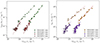 |
Fig. 11. Relation of millimeter emission with SFR and H2. Left: Correlations between the surface densities of the SFR (ΣSFR) and the observed millimeter luminosity (ΣLmm) at 1.15 mm (circles) and 2 mm (triangles) in NGC 2146 (green) and NGC 2976 (red). The lines show the OLS-bisector fits (see Table 8). Right: Same as the left, but for the surface density of molecular gas (ΣH2) as the Y-axis. The maps are smoothed to one pixel per 18″ beam width to prevent internal correlation between pixels. The error bars indicate 1σrms noise of each map, and when not shown, it means that they are smaller than the symbol size. |
Relation of different components of millimeter emission with SFR and H2.
As shown in Fig. 11 and Table 8, there is a strong correlation between ΣSFR and ΣLmm at both wavelengths and in both galaxies, although the correlations are tighter in NGC 2146. The relation of ΣSFR versus the millimeter emission is super-linear, particularly in the case of the dwarf galaxy NGC 2976. In other words, the NIKA2 millimeter maps do not increase linearly with the SFR. Exploring possible sources of this super-linearity, the correlations with the different components of the millimeter emission (RC and dust) are also investigated separately. In all cases, there is a strong correlation; however, a linear correlation is found only with the emission from the RC component, ΣLRC, at both millimeter wavelengths and in both galaxies (Table 8). Linear ΣSFR − ΣLRC is expected since the millimeter RC emission is dominated by the free-free emission, which is a linear tracer of the SFR. On the other hand, the correlation of ΣSFR with the dust component of the millimeter emission, ΣLdust, is not only super-linear, but also has the steepest fitted slope (in the log−log plane) in each galaxy. The super-linearity occurs as ΣLSFR drops faster than ΣLdust toward the low surface density tail of dust emission (or an excess of ΣLdust-to-ΣLSFR). Hence, the millimeter dust emission from galaxies must be partly produced by a diffuse or extended component that is heated by a diffuse ISRF instead of young massive stars. The super-linearity of the ΣSFR − ΣLmm correlation is then linked to the extended dust component. We note that the relation is much steeper in NGC 2976 than in NGC 2146 (Table 8). The more significant contribution of dust than the RC emission (as SFR tracer) in NGC 2976 than NGC 2146 (Sects. 5.1.2 and 5.2.2) can lead to this difference if a significant portion of dust is diffuse, more extended in NGC 2976 compared to that in NGC 2146. A relative excess of dust-to-RC emission in this dwarf galaxy is also evident by comparing its global SED in the centimeter to submillimeter range to that of NGC 2164 (Fig. 5). An excess of extended cold dust emission was also reported in the LMC by Galliano et al. (2011).
Cold dust emission is often used to trace the gas content of galaxies (Boulanger et al. 1996; Bianchi et al. 2022). Although the millimeter correlation with the SFR already implies a correlation with gas (due to the Kennicutt–Schmidt relation), we also investigated the relations between NIKA2 emission at 1.15 and 2 mm with molecular gas.
Figure 11-right shows the molecular gas mass surface density, ΣH2, plotted against ΣLmm (from νLν). The Pearson correlation coefficients and slopes of the best-fit lines are listed in Table 8. In NGC 2146, the correlation coefficients between ΣH2 and the millimeter components agree within the errors. The correlation is always linear with ΣLRC and super-linear with ΣLdust at both millimeter wavelengths. In NGC 2976, ΣH2 is well correlated with the millimeter emission components, although the scatter is larger with dust than with RC.
Overall, the slopes of the ΣH2 correlations with millimeter emission and its components are consistent with those of ΣSFR within the errors as expected from the Kennicutt–Schmidt relation. We note that, in NGC 2146, the correlations of both ΣSFR and ΣH2 with ΣLmm are flatter and closer to linearity at 2 mm than at 1.15 mm which can be explained by a larger contribution of the RC emission at that longer wavelength in this starburst galaxy.
As discussed, the different correlations in these two galaxies simply reflect their very different properties such as the ISM density and dustiness, radiation field, and metallicity. A more general overview of the effect of these properties on the millimeter emission in galaxies, including normal star-forming spirals, will be presented in the forthcoming IMEGIN papers.
6.2. Interplay of dust and gas in NGC 2976
In this section we present how we obtained the total neutral gas content of NGC 2976, explore the correlation of dust and neutral gas components, and investigate the role of dust in the formation of molecular gas in the ISM of this galaxy. As explained in Sect. 2.2, this analysis was not done for NGC 2146 due to a lack of suitable HI data.
6.2.1. Neutral gas and distribution of DGR
The total gas mass is a sum of the molecular gas mass MH2 and the atomic gas mass MHI, that is Mgas = MHI + MH2 (we neglect the relatively small amount of ionized gas). To compute MH2 in NGC 2976, we used the emission of the CO(2−1) line as a well-known tracer and used the relation explained in Sect. 6.1. We report a total molecular gas mass of 7.3 × 10⁷ M⊙ throughout the map, consistent with the value reported in Leroy et al. (2009). Inside our working aperture (i.e., for pixels above the 3σrms noise level of the NIKA2 1.15 mm map), we find a total molecular hydrogen mass of  in NGC 2976.
To estimate the atomic gas mass, we first convolved and regridded the HI map to our working resolution and geometry. Then we converted the flux density of HI to the mass of HI in each pixel using MHI [M⊙] = 2.36 × 10⁵ D2 IHI [Jy/beam m/s], with D the distance to NGC 2976 in megaparsec (Walter et al. 2008). We computed the total HI mass over the whole map to be 1.4 × 10⁸ M⊙ (consistent with the value reported in Walter et al. 2008). We find a total atomic hydrogen mass of MHI = 3.9 × 10⁷ M⊙ in the same regions of the H2 mass determination. After computing the masses of both molecular and atomic gas, the total neutral gas mass was derived in each pixel for NGC 2976.
Knowing the gas and dust mass per pixel, we created a map of the dust-to-gas ratio (DGR), as shown in Fig. 12. The DGR varies from 0.004 to 0.009 in NGC 2976. On average, the DGR is 0.006 ± 0.001 (the error is the standard deviation). Integrating the dust mass in the same way as for the gas mass explained above and dividing them by each other, we find a global value of the DGR equal to 0.006, which equals the mean DGR. These results agree with the DGR values reported by Sandstrom et al. (2013) for NGC 2976 within error margins.
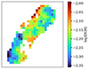 |
Fig. 12. Map of the dust-to-gas mass ratio (DGR) in logarithmic scale, log(Mdust/Mgas) at > 3σrms level at 18″ angular resolution in NGC 2976. |
6.2.2. Molecular and atomic gas fractions
In this section we investigate the relations between the different gas components and dust. The analysis uses independent pixels of beam size (> 3σrms) to prevent internal correlation between the data points. Figure 13 shows that the masses of both atomic MHI and molecular MH2 gas increase as the total (cold + warm) dust mass Mdust increases. However, MHI increases with a smaller slope in the log−log plane (slope ∼1) than MH2 (slope ∼2). Figure 13 shows that as we move from regions with low dust masses to regions with high dust masses, MHI increases by a factor of about 3, while MH2 increases by a factor of approximately 10, which is three times larger. It is inferred from Fig. 13 that although gas is mixed with dust in the ISM of galaxies, and hence shows a positive correlation, different gas components have different relations with dust. Therefore, moving from low dust mass regions to high dust mass regions, the amount of molecular gas increases faster with the amount of dust. Figure 14 shows this relation more evidently, in which the ratio of molecular gas to atomic gas, MH2/MHI, is plotted against the dust mass, Mdust, and ΣSFR is shown as the color scale. At the bottom left of the plot, where dust masses are minimal, atomic gas mass is almost twice the molecular gas mass. However, moving from low dust mass regions to high dust mass areas in the top right corner of the plot, the ratio MH2/MHI increases from 0.5 to more than 1.5. This trend is accompanied by an increase in star formation activity. This indicates that in regions characterized by high dust mass and intense star formation activity, the contribution from molecular gas is almost twice that of atomic gas.
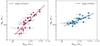 |
Fig. 13. Relation of atomic gas mass MHI (blue) and molecular gas mass MH2 (pink) with dust mass Mdust in NGC 2976. A 3σrms cutoff is applied on the included pixels. The lines show OLS-bisector fits; the slopes are indicated in the insets (see also Table 9). |
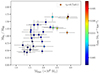 |
Fig. 14. Ratio of molecular to atomic gas mass (MH2/MHI) vs dust mass (Mdust) color-coded according to SFR surface density in NGC 2976. |
6.2.3. Formation and dissociation of H2
Reach & Boulanger (1998) proposed that in relatively cold and dense phases of atomic gas, where the formation and destruction of H2 molecules are balanced, the column density of H2 should change with the column density of HI to a power of 2. Nieten et al. (2006) and Tabatabaei & Berkhuijsen (2010) found such a relationship in M 31, which suggested that a balance in the formation and dissociation of hydrogen molecules holds on average in the ISM of this galaxy. Investigating this in NGC 2976, we find that H2 is proportional to HI to a power smaller than 2 (1.40 ± 0.30, see Table 9). This indicates that the formation and destruction of hydrogen molecules are imbalanced in NGC 2976. This refers to a different ISM condition than that found in M 31 because of which a relatively cold and dense phase of atomic gas in balance with H2 is not easily maintained. This agrees with other studies showing that, in dwarf galaxies, the fraction of the H2 mass fraction, which is sensitive to the dust-to-gas ratio and the strength of the interstellar radiation field is out of chemical equilibrium (Hu et al. 2016) and the formation of hydrogen molecules is less efficient than in dustier spirals (Hirashita & Harada 2017; Hunter et al. 2024).
Relation between different gas components and dust.
7. Summary
In this work we present the first NIKA2 millimeter observations of two nearby galaxies, NGC 2146 (a starburst spiral) and NGC 2976 (a peculiar dwarf), at 1.15 mm and 2 mm, as part of the Guaranteed Time Large Project IMEGIN. These observations provide robust resolved information about the dust physical properties by constraining their FIR-radio SED in the millimeter domain. After subtracting the contribution from the CO line emission, the SEDs were modeled both globally and locally within galaxies using a Bayesian approach. We utilized a double-component MBB model with a variable βc in the global analysis, while keeping it constant for the resolved analysis, as a first-order approximation. This resulted in the generation of cold and warm dust mass, temperature, and free-free fraction maps of these galaxies, allowing us to decompose the components of the millimeter emission and study the relations between the properties of dust and gas. We summarize our main findings as follows:
-
The millimeter emission at 1.15 mm is contaminated by the CO(2−1) line emission by 20% (5%) in NGC 2146 (NGC 2976) on average, with a maximum variation of ∼30% (∼10%) across these galaxies.
-
Studying the global IR to radio SEDs, we find that a dust component with a temperature of ∼32 K constitutes more than 99% of the total dust mass in NGC 2146. A similar portion of the dust in NGC 2976 is found at lower temperatures ∼27 K, making up the majority of the total dust. With a total dust mass lower than that of NGC 2146 by two orders of magnitude, NGC 2976 has a dust emissivity index βc ≃ 1.3, which is flatter than that of NGC 2146 βc ≃ 1.7, as expected for a low-metallicity dwarf galaxy.
-
The global millimeter emission of these galaxies is dominated by dust (∼88%) at 1.15 mm. At 2 mm this contribution decreases to less than 50% in NGC 2146, while it remains almost unchanged in NGC 2976.
-
The pixel-by-pixel SED analysis shows that the dust temperature is generally higher in the inner disk in NGC 2146 and in the star-forming regions in NGC 2976. Cold and warm dust components exhibit similar distributions in the two galaxies, although the warm (minor) component shows a larger fluctuation.
-
By computing the total gas content of NGC 2976, we present a map of the DGR in this galaxy. The DGR ranges between 0.004 and 0.1, while its mean value is 0.006 ± 0.001. We show that the contribution from molecular gas is almost twice that of atomic gas in regions characterized by high dust mass and intense star formation activity. In addition, there is no global balance between the formation and dissociation of H2 in this dwarf galaxy.
-
Tight but super-linear correlations are present between ΣSFR and the millimeter emission in general. Similarly, ΣH2 is well correlated with millimeter emission in both galaxies. As ΣSFR–RC correlation is almost linear, the super-linear correlation of ΣSFR with the millimeter emission is linked to its super-linear correlation with dust. A diffuse distribution of the millimeter dust emission can explain the super-linearity of its correlation with ΣSFR.
Finally, we emphasize that the different results obtained for NGC 2146 (starburst) and NGC 2976 (peculiar dwarf) can be linked to their very different natures, stellar masses, SFRs, and ISM properties. Similar studies in normal and intermediate-mass spirals will shed light on this in the forthcoming IMEGIN papers.
We set Te equal to 104 K, and we note that changing Te from 104 K to 5000 K results in ≲3% difference in A1.
Acknowledgments
We thank the IRAM staff for their support during the observation campaigns. The NIKA2 dilution cryostat has been designed and built at the Institut Néel. In particular, we acknowledge the crucial contribution of the Cryogenics Group, in particular Gregory Garde, Henri Rodenas, Jean-Paul Leggeri, and Philippe Camus. The Foundation Nanoscience Grenoble and the LabEx FOCUS ANR-11-LABX-0013 have partially funded this work. This work is supported by the French National Research Agency under the contracts “MKIDS”, “NIKA” and ANR-15-CE31-0017 and in the framework of the “Investissements d’avenir” program (ANR-15-IDEX-02). This work is supported by the Programme National Physique et Chimie du Milieu Interstellaire (PCMI) and the Programme National Cosmology et Galaxies (PNCG) of the CNRS/INSU with INC/INP co-funded by CEA and CNES. This work has benefited from the support of the European Research Council Advanced Grant ORISTARS under the European Union’s Seventh Framework Programme (Grant Agreement no. 291294). A. R. acknowledges financial support from the Italian Ministry of University and Research – Project Proposal CIR01_00010. S. K. acknowledges support from the Hellenic Foundation for Research and Innovation (HFRI) under the 3rd Call for HFRI PhD Fellowships (Fellowship Number: 5357). M.B., A.N., and S.C.M. acknowledge support from the Flemish Fund for Scientific Research (FWO-Vlaanderen, research project G0C4723N). MME acknowledges the support of the French Agence Nationale de la Recherche (ANR), under grant ANR-22-CE31-0010. This work made use of HERACLES, ‘The HERA CO-Line Extragalactic Survey’ (Leroy et al. 2009). DustPedia is a collaborative focused research project supported by the European Union under the Seventh Framework Programme (2007–2013) call (proposal no. 606847). The participating institutions are Cardiff University, UK; National Observatory of Athens, Greece; Ghent University, Belgium; Université Paris Sud, France; National Institute for Astrophysics, Italy and CEA, France.
References
- Abdo, A. A., Ackermann, M., Ajello, M., et al. 2010, ApJ, 710, 133 [Google Scholar]
- Adam, R., Adane, A., Ade, P. A. R., et al. 2018, A&A, 609, A115 [NASA ADS] [CrossRef] [EDP Sciences] [Google Scholar]
- Akritas, M. G., & Bershady, M. A. 1996, ApJ, 470, 706 [Google Scholar]
- Aniano, G., Draine, B. T., Calzetti, D., et al. 2012, ApJ, 756, 138 [Google Scholar]
- Aniano, G., Draine, B. T., Hunt, L. K., et al. 2020, ApJ, 889, 150 [NASA ADS] [CrossRef] [Google Scholar]
- Asplund, M., Grevesse, N., Sauval, A. J., & Scott, P. 2009, ARA&A, 47, 481 [NASA ADS] [CrossRef] [Google Scholar]
- Baes, M., Clemens, M., Xilouris, E. M., et al. 2010, A&A, 518, L53 [NASA ADS] [CrossRef] [EDP Sciences] [Google Scholar]
- Bendo, G. J., Boselli, A., Dariush, A., et al. 2012, MNRAS, 419, 1833 [NASA ADS] [CrossRef] [Google Scholar]
- Bendo, G. J., Beswick, R. J., D’Cruze, M. J., et al. 2015, MNRAS, 450, L80 [NASA ADS] [CrossRef] [Google Scholar]
- Bendo, G. J., Henkel, C., D’Cruze, M. J., et al. 2016, MNRAS, 463, 252 [NASA ADS] [CrossRef] [Google Scholar]
- Bianchi, S., Murgia, M., Melis, A., et al. 2022, Eur. Phys. J. Web Conf., 257, 00005 [CrossRef] [EDP Sciences] [Google Scholar]
- Boquien, M., Calzetti, D., Combes, F., et al. 2011, AJ, 142, 111 [CrossRef] [Google Scholar]
- Boulanger, F., Abergel, A., Bernard, J. P., et al. 1996, A&A, 312, 256 [Google Scholar]
- Braun, R., Oosterloo, T. A., Morganti, R., Klein, U., & Beck, R. 2007, A&A, 461, 455 [NASA ADS] [CrossRef] [EDP Sciences] [Google Scholar]
- Bron, E., Le Bourlot, J., & Le Petit, F. 2014, A&A, 569, A100 [NASA ADS] [CrossRef] [EDP Sciences] [Google Scholar]
- CASA Team (Bean, B., et al.) 2022, PASP, 134, 114501 [NASA ADS] [CrossRef] [Google Scholar]
- Chen, G., Bendo, G. J., Fuller, G. A., Henkel, C., & Kong, X. 2023, MNRAS, 525, 3645 [NASA ADS] [CrossRef] [Google Scholar]
- Clark, C. J. R., Verstocken, S., Bianchi, S., et al. 2018, A&A, 609, A37 [NASA ADS] [CrossRef] [EDP Sciences] [Google Scholar]
- Condon, J. J. 1992, ARA&A, 30, 575 [Google Scholar]
- de Vaucouleurs, G., de Vaucouleurs, A., Corwin, H. G., et al. 1991, Third Reference Catalogue of Bright Galaxies (New York: Springer-Verlag) [Google Scholar]
- De Vis, P., Jones, A., Viaene, S., et al. 2019, A&A, 623, A5 [NASA ADS] [CrossRef] [EDP Sciences] [Google Scholar]
- Drabek, E., Hatchell, J., Friberg, P., et al. 2012, MNRAS, 426, 23 [Google Scholar]
- Draine, B. T. 2011, Physics of the Interstellar and Intergalactic Medium (Princeton: Princeton University Press) [Google Scholar]
- Draine, B. T., Dale, D. A., Bendo, G., et al. 2007, ApJ, 663, 866 [NASA ADS] [CrossRef] [Google Scholar]
- Engelbracht, C. W., Rieke, G. H., Gordon, K. D., et al. 2008, ApJ, 678, 804 [NASA ADS] [CrossRef] [Google Scholar]
- Foreman-Mackey, D., Hogg, D. W., Lang, D., & Goodman, J. 2013, PASP, 125, 306 [Google Scholar]
- Galametz, M., Madden, S., Galliano, F., et al. 2009, A&A, 508, 645 [NASA ADS] [CrossRef] [EDP Sciences] [Google Scholar]
- Galametz, M., Madden, S. C., Galliano, F., et al. 2011, A&A, 532, A56 [NASA ADS] [CrossRef] [EDP Sciences] [Google Scholar]
- Galametz, M., Kennicutt, R. C., Calzetti, D., et al. 2013, MNRAS, 431, 1956 [NASA ADS] [CrossRef] [Google Scholar]
- Galliano, F. 2022, Habilitation Thesis, Université Paris-Saclay, France [Google Scholar]
- Galliano, F., Madden, S. C., Jones, A. P., et al. 2003, A&A, 407, 159 [NASA ADS] [CrossRef] [EDP Sciences] [Google Scholar]
- Galliano, F., Hony, S., Bernard, J. P., et al. 2011, A&A, 536, A88 [NASA ADS] [CrossRef] [EDP Sciences] [Google Scholar]
- Galliano, F., Galametz, M., & Jones, A. P. 2018, ARA&A, 56, 673 [Google Scholar]
- Galliano, F., Nersesian, A., Bianchi, S., et al. 2021, A&A, 649, A18 [EDP Sciences] [Google Scholar]
- Gao, Y., & Solomon, P. M. 2004, ApJS, 152, 63 [Google Scholar]
- Gil de Paz, A., Boissier, S., Madore, B. F., et al. 2007, ApJS, 173, 185 [Google Scholar]
- Gould, R. J., & Salpeter, E. E. 1963, ApJ, 138, 393 [NASA ADS] [CrossRef] [Google Scholar]
- Greve, A., Neininger, N., Tarchi, A., & Sievers, A. 2000, A&A, 364, 409 [NASA ADS] [Google Scholar]
- Hao, C.-N., Kennicutt, R. C., Johnson, B. D., et al. 2011, ApJ, 741, 124 [Google Scholar]
- Heesen, V., Staffehl, M., Basu, A., et al. 2022, A&A, 664, A83 [NASA ADS] [CrossRef] [EDP Sciences] [Google Scholar]
- Hirashita, H., & Harada, N. 2017, MNRAS, 467, 699 [NASA ADS] [Google Scholar]
- Hu, C.-Y., Naab, T., Walch, S., Glover, S. C. O., & Clark, P. C. 2016, MNRAS, 458, 3528 [CrossRef] [Google Scholar]
- Hunt, L. K., García-Burillo, S., Casasola, V., et al. 2015, A&A, 583, A114 [NASA ADS] [CrossRef] [EDP Sciences] [Google Scholar]
- Hunt, L. K., De Looze, I., Boquien, M., et al. 2019, A&A, 621, A51 [NASA ADS] [CrossRef] [EDP Sciences] [Google Scholar]
- Hunter, D. A., Elmegreen, B. G., & Madden, S. C. 2024, ARA&A, 62, 113 [NASA ADS] [CrossRef] [Google Scholar]
- James, P. A., Shane, N. S., Beckman, J. E., et al. 2004, A&A, 414, 23 [NASA ADS] [CrossRef] [EDP Sciences] [Google Scholar]
- Juvela, M., & Ysard, N. 2012, A&A, 539, A71 [NASA ADS] [CrossRef] [EDP Sciences] [Google Scholar]
- Katsioli, S., Xilouris, E. M., Kramer, C., et al. 2023, A&A, 679, A7 [CrossRef] [EDP Sciences] [Google Scholar]
- Kelly, B. C., Shetty, R., Stutz, A. M., et al. 2012, ApJ, 752, 55 [NASA ADS] [CrossRef] [Google Scholar]
- Kennicutt, R. C., & Evans, N. J. 2012, ARA&A, 50, 531 [NASA ADS] [CrossRef] [Google Scholar]
- Kennicutt, R. C., Armus, L., Bendo, G., et al. 2003, PASP, 115, 928 [NASA ADS] [CrossRef] [Google Scholar]
- Kennicutt, R. C., Calzetti, D., Aniano, G., et al. 2011, PASP, 123, 1347 [Google Scholar]
- Kramer, C., Buchbender, C., Quintana-Lacaci, G., et al. 2010, Highlights Astron., 15, 415 [NASA ADS] [Google Scholar]
- Kreckel, K., Armus, L., Groves, B., et al. 2014, ApJ, 790, 26 [NASA ADS] [CrossRef] [Google Scholar]
- Kroupa, P., & Weidner, C. 2003, ApJ, 598, 1076 [NASA ADS] [CrossRef] [Google Scholar]
- Leroy, A. K., Walter, F., Bigiel, F., et al. 2009, AJ, 137, 4670 [Google Scholar]
- Leroy, A. K., Walter, F., Sandstrom, K., et al. 2013, AJ, 146, 19 [Google Scholar]
- Michiyama, T., Iono, D., Nakanishi, K., et al. 2020, ApJ, 895, 85 [Google Scholar]
- Nersesian, A., Xilouris, E. M., Bianchi, S., et al. 2019, A&A, 624, A80 [NASA ADS] [CrossRef] [EDP Sciences] [Google Scholar]
- Nieten, C., Neininger, N., Guélin, M., et al. 2006, A&A, 453, 459 [CrossRef] [EDP Sciences] [Google Scholar]
- Niklas, S., Klein, U., Braine, J., & Wielebinski, R. 1995, A&AS, 114, 21 [NASA ADS] [Google Scholar]
- Orellana, G., Nagar, N. M., Elbaz, D., et al. 2017, A&A, 602, A68 [NASA ADS] [CrossRef] [EDP Sciences] [Google Scholar]
- Peel, M. W., Dickinson, C., Davies, R. D., Clements, D. L., & Beswick, R. J. 2011, MNRAS, 416, L99 [NASA ADS] [CrossRef] [Google Scholar]
- Perets, H. B., & Biham, O. 2006, MNRAS, 365, 801 [NASA ADS] [CrossRef] [Google Scholar]
- Perotto, L., Ponthieu, N., Macías-Pérez, J. F., et al. 2020, A&A, 637, A71 [NASA ADS] [CrossRef] [EDP Sciences] [Google Scholar]
- Pettini, M., & Pagel, B. E. J. 2004, MNRAS, 348, L59 [NASA ADS] [CrossRef] [Google Scholar]
- Pilyugin, L. S., & Grebel, E. K. 2016, MNRAS, 457, 3678 [NASA ADS] [CrossRef] [Google Scholar]
- Planck Collaboration I. 2014, A&A, 571, A1 [NASA ADS] [CrossRef] [EDP Sciences] [Google Scholar]
- Pope, A., Chary, R.-R., Alexander, D. M., et al. 2008, ApJ, 675, 1171 [Google Scholar]
- Reach, W. T., & Boulanger, F. 1998, in IAU Colloq. 166: The Local Bubble and Beyond, eds. D. Breitschwerdt, M. J. Freyberg, & J. Truemper, 506, 353 [NASA ADS] [Google Scholar]
- Rémy-Ruyer, A., Madden, S. C., Galliano, F., et al. 2013, A&A, 557, A95 [Google Scholar]
- Roussel, H. 2013, PASP, 125, 1126 [Google Scholar]
- Roussel, H., Ponthieu, N., Adam, R., et al. 2020, Eur. Phys. J. Web Conf., 228, 00024 [CrossRef] [EDP Sciences] [Google Scholar]
- Salak, D., Tomiyasu, Y., Nakai, N., et al. 2017, ApJ, 849, 90 [NASA ADS] [CrossRef] [Google Scholar]
- Sandstrom, K. M., Leroy, A. K., Walter, F., et al. 2013, ApJ, 777, 5 [Google Scholar]
- Schruba, A., Leroy, A. K., Walter, F., et al. 2011, AJ, 142, 37 [NASA ADS] [CrossRef] [Google Scholar]
- Shetty, R., Kauffmann, J., Schnee, S., & Goodman, A. A. 2009, ApJ, 696, 676 [NASA ADS] [CrossRef] [Google Scholar]
- Smith, J. D. T., Draine, B. T., Dale, D. A., et al. 2007, ApJ, 656, 770 [Google Scholar]
- Tabatabaei, F. S., & Berkhuijsen, E. M. 2010, A&A, 517, A77 [NASA ADS] [CrossRef] [EDP Sciences] [Google Scholar]
- Tabatabaei, F. S., Weiß, A., Combes, F., et al. 2013a, A&A, 555, A128 [NASA ADS] [CrossRef] [EDP Sciences] [Google Scholar]
- Tabatabaei, F. S., Schinnerer, E., Murphy, E. J., et al. 2013b, A&A, 552, A19 [NASA ADS] [CrossRef] [EDP Sciences] [Google Scholar]
- Tabatabaei, F. S., Braine, J., Xilouris, E. M., et al. 2014, A&A, 561, A95 [NASA ADS] [CrossRef] [EDP Sciences] [Google Scholar]
- Tabatabaei, F. S., Schinnerer, E., Krause, M., et al. 2017, ApJ, 836, 185 [Google Scholar]
- Taramopoulos, A., Payne, H., & Briggs, F. H. 2001, A&A, 365, 360 [NASA ADS] [CrossRef] [EDP Sciences] [Google Scholar]
- Tarchi, A., Greve, A., Peck, A. B., et al. 2004, MNRAS, 351, 339 [NASA ADS] [CrossRef] [Google Scholar]
- Tielens, A. G. C. M. 1997, ASP Conf. Ser., 124, 255 [NASA ADS] [Google Scholar]
- Valenzuela, O., Hernandez-Toledo, H., Cano, M., et al. 2014, AJ, 147, 27 [Google Scholar]
- Walter, F., Brinks, E., de Blok, W. J. G., et al. 2008, AJ, 136, 2563 [Google Scholar]
- Ysard, N., Jones, A. P., Guillet, V., et al. 2024, A&A, 684, A34 [NASA ADS] [CrossRef] [EDP Sciences] [Google Scholar]
Appendix A: Data processing
A.1. Recalibration of detector gains and beam solid angles
The flux calibration is applied through the NIKA2 pipeline according to the analysis presented in Perotto et al. (2020) which is strictly valid only for point sources. In addition, the response of individual detectors to extended emission is corrected, by using the atmospheric emission in the raw data of the science observations themselves as a template of very extended emission. This is possible whenever the scan duration is longer than about 5 min and the sources (to be masked in the process) occupy a small fraction of the map. Both conditions are met in the IMEGIN observations. The gains are very stable on the timescale of an observing pool.
All Uranus beam maps (large maps in the azimuth direction, with optimal redundancy provided by a fine sampling in elevation) acquired within 19 runs from October 2017 to January 2023, spanning all IMEGIN observations, were reduced and analyzed to monitor variations of the beam solid angle during that period. With an aperture size of 2.5 FWHM (2 mm), corresponding to twice the half-power beam width (HPBW) in maps of both bands convolved to the same angular resolution (a compromise for maps containing a mixture of compact sources and diffuse emission), and excluding the outlier run 50 (December 2019), we found effective beam solid angles Ωeff(1.15 mm) = (188 ± 11) arcsec2 and Ωeff(2 mm) = (381 ± 11) arcsec2, corresponding to rms flux calibration uncertainties of 5.9% at 1.15 mm and 2.9% at 2 mm. The rms uncertainty is in line with that Perotto et al. (2020) derived from three reference runs at both wavelengths.
A.2. Processing of NIKA2 data
The NIKA2 data were processed with the Scanam_nika software, adapted from Scanamorphos originally developed for Herschel on-the-fly imaging data. The underlying principle is to fully exploit the redundancy built in the observations (each sky position within the nominal-coverage area being sampled by multiple detectors at multiple times, and in variable atmospheric conditions) while making minimal assumptions about the atmospheric and instrumental noise, as described by Roussel (2013) and Roussel et al. (2020). The low-frequency noise, or drift, is decomposed into the following components:
-
the average drift time series averaged over all valid detectors, each one weighted by its inverse variance at the highest frequencies;
-
the drift per electronic box time series, averaged over all valid detectors of each of the 4 (2 mm) or 16 (1.15 mm) electronic boxes; and the equivalent component obtained by artificially slicing the detector arrays into the same number of boxes, but orthogonal to the physical boxes;
-
the individual noise time series (one function of time for each detector);
-
the noise series not as a function of time, but binned per position on the sky along the array trajectory, projected on the long axis of the electronic boxes; and the equivalent component projected on the short axis of the electronic boxes.
The latter components were introduced to remove a significant residual noise remaining after subtraction of the other correlated noise components and found empirically by the resemblance of their spatial pattern in the map with that of standing waves. They correspond to a genuine electronic noise best seen in instrumental coordinates, arising in the cryostat (internal NIKA2 communication from F.X. Désert and N. Ponthieu, March 2023).
The minimum timescale of the drifts, tc, is determined by the stability length and the scanning speed (see Roussel 2013). The average drift is subtracted on this timescale, while the other drift components are subtracted on successively smaller or larger timescales, multiples of tc.
The process is iterative and uses a source mask that is automatically updated at each iteration, as the sources gradually emerge from the decreasing residual noise. The mask is always constrained to be confined within a 5σrms isophote in the SPIRE 500 μm map, to avoid contamination by spurious structures created by noise.
At the end of the processing, the median surface brightness of the sky and σrms are calculated in the area of the field with optimal coverage, excluding the pixels contained within the final source mask. The sky level is then subtracted from the map.
A.3. Simulations for homogeneous dust SEDs from instruments with dissimilar transfer functions
The astrophysical signal at 1.15 and 2 mm is filtered in a complex way, depending on the atmospheric conditions and stability at the time of observations, source brightness and geometry, observation parameters such as scanning speed, scan geometry, and the processing algorithm. In general, sources bigger than the instantaneous FoV of NIKA2 (6.5′) as well as regions with low signal-to-noise ratios are filtered due to those effects. By contrast, all spatial scales smaller than the map size can be accurately recovered with the Herschel and Spitzer space observatories. Hence, to build coherent spatially resolved dust SEDs traced from 24 μm to 2 mm, this discrepancy has to be mitigated: the Herschel and Spitzer maps have to be filtered in the same way as the NIKA2 maps. The ratio of the sky map that is obtained to the map that would be obtained by a perfect instrument outside the atmosphere is hereafter called the transfer function. We chose to apply the transfer function of NIKA2 at 2 mm (assuming that it is equivalent to that at 1.15 mm, since the observations in both bands are simultaneous) to all observations of dust from space. For a given Herschel/Spitzer band, the process is the following:
-
convolve the map with a Gaussian kernel to bring it approximately to the same FWHM as that of the 2 mm map (except at 350 and 500 μm);
-
correct for any small astrometric offset between the maps, by fitting the brightest compact source with a Gaussian for each band;
-
rescale the map so that the ratio of the MIPS or Herschel band to the 2 mm band has a median of 1 within the galaxy extent;
-
simulate time series from the map as if it had been observed with NIKA2 with the same scan geometry and duration;
-
add to these time series the low-frequency and high-frequency noise that was extracted from the 2 mm data (drifts, glitches, etc.) and a realization of the white noise present in the 2 mm data;
-
process these time series in the same way as the NIKA2 data and project the result on the same spatial grid;
-
rescale the map back to its original unit.
The comparison of the simulated output map with the initial map directly gives the spatially resolved transfer function, and it can be checked that it is very similar for all Spitzer and Herschel bands. In addition, for these small galaxies, it is very close to unity in all signal-to-noise ratio bins, as shown in Fig. A.1.
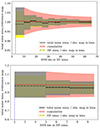 |
Fig. A.1. Transfer functions at 250 μm (with a FWHM of 18″) binned as a function of signal-to-noise ratio (S/N) where the noise standard deviation σHF is from a simulation including only white and high-frequency noise. The red curve and red shaded area show the cumulative fraction of the flux that is recovered and the associated uncertainties, from the lower S/N limit (3σHF for NGC 2146 and 2σHF for NGC 2976) up to the maximum of the current S/N bin. |
The main benefit of applying the NIKA2 transfer function to the other bands, instead of using the original maps, is then to homogenize the noise properties across the dust SED, so that the parameters extracted from the SED fits are as unbiased as possible. The NIKA2 transfer function was not applied to the UV, optical, and gas maps, because these data are not used in SED fitting. Therefore, it is irrelevant that their noise properties are inhomogeneous, since for these two galaxies, the only significant effect of applying the NIKA2 transfer function is to alter the noise properties, and not to alter the flux.
Appendix B: CO contamination
The emission measured at 1.15 mm with NIKA2 consists mainly of continuum emission and partly of the CO(2-1) line emission. This is caused by the fact that the NIKA2 passband includes the CO (2-1) emission line at 230.5 GHz. In this section we explain how we compute the amount of this contamination and subtract it from the total observed continuum emission to obtain pure dust emission in the 1.15 mm NIKA2 band for the SED modeling.
The CO(2-1) line intensity is measured in units of the main beam temperature, while the continuum flux density is measured in units of mJy/beam. We follow the procedure explained in Drabek et al. (2012) to convert from K km/s to mJy/beam
 (B.1)
(B.1)
where Fν is the line flux density and ICO = ∫TMB dv is velocity integrated main beam temperature of the CO(2-1) line emission in units K km s−1, and C is the conversion factor. This is equivalent to
 (B.2)
(B.2)
In the above equation, k is Boltzmann’s constant, ν is the line frequency, ΩB is the solid angle corresponding to NIKA2 beam area, and gν(line) is the transmission function at the molecular line frequency and ∫gν dν is the integral of the transmission function of the NIKA2 1.15 mm detector over the whole range of filter frequencies, Perotto et al. (2020). We find the value of  by integrating on the NIKA2 1.15 mm pass-band and find it to be 7.85 × 10⁻³ GHz−1. Also, the beam area corresponding to our working resolution of 18″ is 8.63 × 10⁻⁹ steradians. We find the conversion factor C to be equal to 0.085 mJy/beam per K km/s for NIKA2 1.15 mm pass-band.
The Planck pass-band at 1.38 mm is also affected by line emission contamination (Planck Collaboration I 2014). We follow a similar procedure to subtract CO(2-1) contamination from the Planck 1.38 mm map before including it in the SED fitting process. Using Eq. B.2 and taking into account Planck’s pass-band and resolution (301″), we find C = 50.6 mJy/beam per K km/s.
Appendix C: Error estimation
The measured integrated flux in each waveband can be subject to different stochastic or systematic uncertainties. We estimate the stochastic error by measuring the rms noise level, σrms, of the maps. The calibration uncertainty of the observations (see Sect. 2) is used to estimate the systematic error. The total error is then
 (C.1)
(C.1)
For the integrated flux densities, δrms is given by
 (C.2)
(C.2)
where σrms is the rms noise level in Jy/beam, Nbeam and N is the number of beams and number of pixels in the aperture, θ the angular resolution and a the pixel size, both in units of arcsec2. We note that because the maps have different resolutions and pixel sizes, N, θ, and a vary for each map (see Table 2).
Appendix D: Model fitting using Bayesian approach
To model the SED, we fit a model with ndim free parameters to ndata data points. For the two galaxies, we have studied, in the global case ndim = 8 and ndata = 14, and in the resolved case ndim = 6 and ndata = 9. In the context of the Bayesian approach, we look for the Probability Distribution Function (PDF) of the posterior p(x|d), which is the PDF of the free parameters, conditional on the data points. The Markov Chain Monte-Carlo (MCMC) method is an algorithm that can sample a PDF -here the posterior. To implement the MCMC method to sample the posterior distribution, we use the emcee Python package (Foreman-Mackey et al. 2013). This package uses a pre-specified number of random walkers (nwalkers) in the parameter space. The parameter space has ndim dimensions and is defined by the prior PDFs. The random walkers explore the parameter space. In each step, the likelihood PDF is computed, which is a function of the absolute difference between the model and the data points at different wavelengths. After the random walkers move a total of nsteps steps, we have an array of length nsteps of the values that each random walker has acquired in each step. This array should be refined in two ways. Firstly, the initial nburn steps are deleted, because they incorporate the initial steps that the random walkers are not close to the best value. Second, this array is filtered by every nthin number to resolve the autocorrelation between the steps. We chose nthin such that the length of the time series produced by random walkers is at least 40 times the autocorrelation function of the time series. We found the value ranges nwalkers = 40, nsteps = 60000 − 100000, and nthin = 200 − 1000 are appropriate for our problem. We assume flat prior PDFs for all free parameters. Also, to be able to sweep all the parameter space, we set the boundaries of our free parameters to be 5K < Tc < 35 K, 35 < Tw < 95, 101 M⊙ < M < 108 M⊙, 0.5 < β < 3.0, −0.01 < A1 < 0.1, −0.001 < A2 < 1, and 0.2 < αn < 2.5.
The joint posterior PDF of random walkers moving in the parameters space is then plotted. This joint PDF is a sample of the posterior PDF of the free parameters, which can be displayed in a corner plot. We report the median value as the resulting value for each free parameter and the 20% and 80% percentiles as the error margins. Since the posterior distributions are not necessarily symmetrical, we report asymmetrical error margins for each parameter in Table 4. Figure D.1 shows the corner plots of the global SED modeling of the two galaxies.
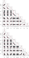 |
Fig. D.1. Corner plots of joint posterior PDFs as a result of the MCMC process, carried out for global SED modeling of (top) NGC 2146 and (bottom) NGC 2976. The median of each distribution function is shown with the red lines. We note that the axis for A1 is in units of 102 for clarity. |
Each step of the random walkers is assigned to a set of values for the ndim free parameters. This set of values results in a value for the model function in that step. Then prediction of this particular model value for each ndata wavelength is compared to the actual observed data points. In other words, in each step, the prediction of the model for ndata wavelengths is computed. To correctly compute the prediction of the model for each wavelength, the likelihood function should be convolved with the transmission function of each instrument. This is essential because we need to know the prediction of the model as observed with each instrument at each wavelength. To have a correct prediction of each instrument in their nominal wavelengths, we implement the transmission function of all the involved instruments in the likelihood function. This process makes the core slower, and we compensate for that by implementing multiprocessing methods.
Figure D.2 presents a compilation of all SEDs for all the pixels, which shows the significance of NIKA2 observations, represented by green dots, in resolved studies. It is evident that without NIKA2 observations, it would be impossible to constrain the trough of the SED in the millimeter regime.
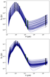 |
Fig. D.2. Compilation of all the SEDs for individual pixels (above 3σrms limit) in NGC 2146 (top) and NGC 2976 (bottom). The green dots show NIKA2 observations. |
All Tables
Contribution of the three constituents of continuum emission with respect to the modeled flux at 1.15 mm and 2 mm.
All Figures
|
Fig. 1. Observed NIKA2 maps of NGC 2146 (top) and NGC 2976 (bottom) at 1.15 mm (left) and 2 mm (right). The color bars show the flux density in units of mJy/beam. The circle in the bottom left corner of each panel indicates the angular resolution (beam widths) which is 12″ and 18″ at 1.15 mm and 2 mm, respectively. The contours show the MIPS 24 μm emission at levels 9, 54, and 324 Jy/pixel in the top panels and 0.8, 2.4, and 7.2 Jy/pixel in the bottom panels. The FoV is 4′×4′ and 5′×5′ for NGC 2146 and NGC 2976, respectively. |
| In the text | |
|
Fig. 2. Complementary data used in this work for NGC 2146. GALEX FUV, Spitzer MIPS, Herschel SPIRE and PACS, radio, and CO(2−1) maps are presented. The optical image in the Red filter displays the optical features of this galaxy and is not used in the analysis. The Planck 1.38 mm and radio 6.2 cm maps are also not shown due to poor resolution. All the demonstrated maps have the same FoV of 3.5′×4′, centered on the galaxy. The maps are displayed in logarithmic scale and their original resolution (see indicated Table 2); the beam size is represented by a white circle in the bottom left corner of each map. |
| In the text | |
|
Fig. 3. Same as Fig. 2, but for NGC 2976. The HI map, which is only available for this galaxy, is also included. The optical map in the Red filter displays the optical features of this galaxy and is not used in the analysis. The Planck 1.38 mm and radio 6.2 cm maps are also not shown due to poor resolution. All the demonstrated maps have the same FoV of 3.7′×4.2′ centered on the galaxy. The maps are all shown in logarithmic scale and at their original resolution (see Table 2); the beam size is represented by a white circle in the bottom left corner of each map. |
| In the text | |
|
Fig. 4. Maps of the CO fraction defined as the ratio of the CO(2−1) line emission to the observed 1.15 mm emission in NGC 2146 (left) and NGC 2976 (right) at 18″ angular resolution. Only pixels above the 3σrms level of the observed NIKA2 map are shown. Contours show the intensity of CO emission in each galaxy, starting from 1σrms and increasing by factors of 3. The circles in the bottom left corners indicate the beam area. |
| In the text | |
|
Fig. 5. Global IR-to-radio SED (solid black curve) and its decomposed individual components of the cold dust (blue dashed curve), warm dust (orange dot-dashed curve), free-free (purple dotted curve), and synchrotron emission (green solid curve) in NGC 2146 (top) and NGC 2976 (bottom). The shaded gray area shows the uncertainty of the model. The relative residual of the model and observations with respect to the observation is shown at the bottom of each plot. The resulting SED parameters are listed in Table 4. |
| In the text | |
|
Fig. 6. IR-to-radio SEDs of a selected pixel in NGC 2146 (top) and NGC 2976 (bottom). The curves show the cold dust (blue dashed curve), warm dust (orange dot-dashed curve), free-free (purple dotted curve), and synchrotron (green solid curve) emissions. |
| In the text | |
|
Fig. 7. Maps of the resulting SED parameters for NGC 2146 for 6″ pixels (≃525 pc). Shown (from left to right) are cold dust temperature Tc (K), cold dust mass surface density |
| In the text | |
|
Fig. 8. Same as Fig. 7, but for NGC 2976. The SED analysis only uses pixels with intensities > 1σrms at all wavelengths for this dwarf galaxy. |
| In the text | |
|
Fig. 9. Contribution percentage from dust (left column), free-free (middle column), and synchrotron (right column) emission in the total modeled flux at 1.15 mm (top row) and 2 mm (bottom row) are shown for NGC 2146 (top panel) and NGC 2976 (bottom panel). |
| In the text | |
|
Fig. 10. Map of pure dust emission at 1.15 mm (after subtraction of the CO line contamination, free-free, and synchrotron emission) in mJy/pixel in NGC 2146 (top) and NGC 2976 (bottom). |
| In the text | |
|
Fig. 11. Relation of millimeter emission with SFR and H2. Left: Correlations between the surface densities of the SFR (ΣSFR) and the observed millimeter luminosity (ΣLmm) at 1.15 mm (circles) and 2 mm (triangles) in NGC 2146 (green) and NGC 2976 (red). The lines show the OLS-bisector fits (see Table 8). Right: Same as the left, but for the surface density of molecular gas (ΣH2) as the Y-axis. The maps are smoothed to one pixel per 18″ beam width to prevent internal correlation between pixels. The error bars indicate 1σrms noise of each map, and when not shown, it means that they are smaller than the symbol size. |
| In the text | |
|
Fig. 12. Map of the dust-to-gas mass ratio (DGR) in logarithmic scale, log(Mdust/Mgas) at > 3σrms level at 18″ angular resolution in NGC 2976. |
| In the text | |
|
Fig. 13. Relation of atomic gas mass MHI (blue) and molecular gas mass MH2 (pink) with dust mass Mdust in NGC 2976. A 3σrms cutoff is applied on the included pixels. The lines show OLS-bisector fits; the slopes are indicated in the insets (see also Table 9). |
| In the text | |
|
Fig. 14. Ratio of molecular to atomic gas mass (MH2/MHI) vs dust mass (Mdust) color-coded according to SFR surface density in NGC 2976. |
| In the text | |
|
Fig. A.1. Transfer functions at 250 μm (with a FWHM of 18″) binned as a function of signal-to-noise ratio (S/N) where the noise standard deviation σHF is from a simulation including only white and high-frequency noise. The red curve and red shaded area show the cumulative fraction of the flux that is recovered and the associated uncertainties, from the lower S/N limit (3σHF for NGC 2146 and 2σHF for NGC 2976) up to the maximum of the current S/N bin. |
| In the text | |
|
Fig. D.1. Corner plots of joint posterior PDFs as a result of the MCMC process, carried out for global SED modeling of (top) NGC 2146 and (bottom) NGC 2976. The median of each distribution function is shown with the red lines. We note that the axis for A1 is in units of 102 for clarity. |
| In the text | |
|
Fig. D.2. Compilation of all the SEDs for individual pixels (above 3σrms limit) in NGC 2146 (top) and NGC 2976 (bottom). The green dots show NIKA2 observations. |
| In the text | |
Current usage metrics show cumulative count of Article Views (full-text article views including HTML views, PDF and ePub downloads, according to the available data) and Abstracts Views on Vision4Press platform.
Data correspond to usage on the plateform after 2015. The current usage metrics is available 48-96 hours after online publication and is updated daily on week days.
Initial download of the metrics may take a while.