| Issue |
A&A
Volume 675, July 2023
BeyondPlanck: end-to-end Bayesian analysis of Planck LFI
|
|
|---|---|---|
| Article Number | A4 | |
| Number of page(s) | 15 | |
| Section | Cosmology (including clusters of galaxies) | |
| DOI | https://doi.org/10.1051/0004-6361/202244958 | |
| Published online | 28 June 2023 | |
BEYONDPLANCK
IV. Simulations and validation
1
Institute of Theoretical Astrophysics, University of Oslo, Blindern, Oslo, Norway
2
Instituto de Física, Universidade de São Paulo, C.P. 66318, CEP:, 05315-970 São Paulo, Brazil
3
Department of Physics and Astronomy, University of British Columbia, Vancouver, BC V6T 1Z1, Canada
4
Astronomical Institute, Tohoku University, Sendai, Miyagi 980-8578, Japan
5
Indian Institute of Astrophysics, Koramangala II Block, Bangalore 560034, India
6
Department of Physics, University of California, Berkeley, Berkeley, CA, USA
7
Instituto Nacional de Pesquisas Espaciais, Divisão de Astrofísica, Av. dos Astronautas, 1758, 12227-010 São José dos Campos, SP, Brazil
8
Department of Physics and Astronomy, University College London, Gower Street, London WC1E 6BT, UK
9
Department of Physics and Electronics, Rhodes University, PO Box 94, Grahamstown 6140, South Africa
10
Planetek Hellas, Leoforos Kifisias 44, Marousi 151 25, Greece
11
Dipartimento di Fisica, Università degli Studi di Milano, Via Celoria, 16, Milano, Italy
12
INAF/IASF Milano, Via E. Bassini 15, Milano, Italy
13
INFN, Sezione di Milano, Via Celoria 16, Milano, Italy
14
INAF – Osservatorio Astronomico di Trieste, Via G.B. Tiepolo 11, Trieste, Italy
15
Department of Astrophysical Sciences, Princeton University, Princeton, NJ 08544, USA
16
Kavli IPMU (WPI), UTIAS, The University of Tokyo, Kashiwa, Chiba 277-8583, Japan
17
Jet Propulsion Laboratory, California Institute of Technology, 4800 Oak Grove Drive, Pasadena, CA, USA
18
Department of Physics, Gustaf Hällströmin katu 2, University of Helsinki, Helsinki, Finland
19
Helsinki Institute of Physics, Gustaf Hällströmin katu 2, University of Helsinki, Helsinki, Finland
20
Computational Cosmology Center, Lawrence Berkeley National Laboratory, Berkeley, CA, USA
21
Haverford College Astronomy Department, 370 Lancaster Avenue, Haverford, Pennsylvania, USA
22
Max-Planck-Institut für Astrophysik, Karl-Schwarzschild-Str. 1, 85741 Garching, Germany
23
Dipartimento di Fisica, Università degli Studi di Trieste, Via A. Valerio 2, Trieste, Italy
Received:
12
September
2022
Accepted:
2
April
2023
End-to-end simulations play a key role in the analysis of any high-sensitivity cosmic microwave background (CMB) experiment, providing high-fidelity systematic error propagation capabilities that are unmatched by any other means. In this paper, we address an important issue regarding such simulations, namely, how to define the inputs in terms of sky model and instrument parameters. These may either be taken as a constrained realization derived from the data or as a random realization independent from the data. We refer to these as posterior and prior simulations, respectively. We show that the two options lead to significantly different correlation structures, as prior simulations (contrary to posterior simulations) effectively include cosmic variance, but they exclude realization-specific correlations from non-linear degeneracies. Consequently, they quantify fundamentally different types of uncertainties. We argue that as a result, they also have different and complementary scientific uses, even if this dichotomy is not absolute. In particular, posterior simulations are in general more convenient for parameter estimation studies, while prior simulations are generally more convenient for model testing. Before BEYONDPLANCK, most pipelines used a mix of constrained and random inputs and applied the same hybrid simulations for all applications, even though the statistical justification for this is not always evident. BEYONDPLANCK represents the first end-to-end CMB simulation framework that is able to generate both types of simulations and these new capabilities have brought this topic to the forefront. The BEYONDPLANCK posterior simulations and their uses are described extensively in a suite of companion papers. In this work, we consider one important applications of the corresponding prior simulations, namely, code validation. Specifically, we generated a set of one-year LFI 30 GHz prior simulations with known inputs and we used these to validate the core low-level BEYONDPLANCK algorithms dealing with gain estimation, correlated noise estimation, and mapmaking.
Key words: cosmic background radiation / cosmology: observations / diffuse radiation
© The Authors 2023
 Open Access article, published by EDP Sciences, under the terms of the Creative Commons Attribution License (https://creativecommons.org/licenses/by/4.0), which permits unrestricted use, distribution, and reproduction in any medium, provided the original work is properly cited.
This article is published in open access under the Subscribe to Open model.
Open Access funding provided by Max Planck Society.
1. Introduction
High-fidelity end-to-end simulations play a critical role in the analysis of any modern cosmic microwave background (CMB) experiment for at least three important reasons. Firstly, during the design phase of the experiment, simulations are used to optimize and forecast the performance of a given experimental design and ensure that the future experiment will achieve its scientific goals (e.g., LiteBIRD Collaboration 2023). Secondly, simulations are essential for validation purposes, since they may be used to test data-processing techniques as applied to a realistic instrument model. Thirdly, realistic end-to-end simulations play an important role in bias and error estimations for traditional CMB analysis pipelines.
Simulations played a particularly important role in the data reduction of Planck and massive efforts were invested in implementing efficient and re-usable analysis codes that were generally applicable to a wide range of experiments. This work started with the LevelS software package (Reinecke et al. 2015) and culminated with the Time Ordered Astrophysics Scalable Tools1 (TOAST), which was explicitly designed to operate in a massively parallel high-performance computing environment. TOAST was used to produce the final generations of the Planck Full Focal Plane (FFP) simulations (Planck Collaboration XII 2016), which served as the main error propagation mechanism in the Planck 2015 and 2018 data releases (Planck Collaboration I 2016, 2020).
For Planck, generating end-to-end simulations have represented (by far) the dominant computational cost of the entire experiment, accounting for 25 million CPU-hrs in the 2015 data release alone. In addition, the production phase required massive amounts of human effort, in terms of preparing the inputs, executing the runs, and validating the outputs. It is of great interest for any future experiment to optimize and streamline this simulation process, and reuse both validated software and human work whenever possible.
In this respect, the BEYONDPLANCK end-to-end Bayesian analysis framework (BeyondPlanck Collaboration 2023) offers a novel approach to generating CMB simulations. While the primary goal of this framework is to draw samples from a full joint posterior distribution for analytical purposes, it is useful to note that the foundation of this approach is simply a general and explicit parametric model for the full time-ordered data (TOD). When exploring the full joint posterior distribution, this model is compared with the observed data in the TOD space. The analysis phase is as such numerically equivalent to producing a large number of TOD simulations and comparing each of these with the actual observed data. In this framework, each step of the analysis and simulation pipelines are thus fully equivalent, and the primary difference is simply based on whether the input model parameters are assumed to be constrained by the data or not.
This latter observation is in fact a key point regarding end-to-end simulations for CMB experiments in general, and a main goal of the current paper is to clarify the importance of choosing input parameters for a given simulation appropriately. Specifically, we argue in this paper that two fundamentally different choices are available: we can either choose parameters that are constrained directly by the observed data (as is traditionally done for the CMB Solar dipole or astrophysical foregrounds) or we can choose parameters that are independent from the observed data (as is traditionally done for CMB fluctuations or instrumental noise). We further argue that this choice will have direct consequences for the specific scientific questions the resulting simulations are optimized to address.
It is important to note that these ideas were discussed broadly, but not systematically, within the Planck community before building the FFP simulations. For instance, one proposal was to base the large-scale CMB temperature fluctuations at ℓ ≤ 70 from constrained WMAP realizations (Bennett et al. 2013), and thereby integrate knowledge about the real sky into the simulations. Another proposal was to use the actually observed LFI gain measurements to generate the simulations. A third and long-standing discussion has revolved around which values to adopt for the CMB Solar dipole.
The BEYONDPLANCK framework offers a novel systematic view on these questions, as our Bayesian approach provides for the first time statistically well-defined constrained realizations for all parameters in the sky model – and not just a small subset. Furthermore, when comparing the correlation structures that arise from the posterior samples with those derived from traditional simulations, obvious and important differences appear, both in terms of the frequency maps (Basyrov et al. 2023) and CMB maps (Colombo et al. 2023).
The first main goal of the current paper is to explain these differences intuitively and in that process, we introduce the concepts of “posterior simulations” and “prior simulations”2. Posterior simulations are random samples drawn from P(ω|d), and represent simulations that are constrained by the observed data; these are thus identical to the posterior samples described by BeyondPlanck Collaboration (2023). In contrast, prior simulations drawn from a prior distribution, P(ω), and are, as such, unconstrained by the data. We note that a similar distinction has recently been made in terms of a so-called “Bayesian workflow” by Betancourt3 and Gelman et al. (2020).
The second main goal of this paper is simply to demonstrate in practice how the BEYONDPLANCK machinery may be used to generate prior simulations, on a similar footing as TOAST, and we will use these simulations for one important application, namely code validation. As discussed by Galloway et al. (2023a) and Gerakakis et al. (2023), the Commander code that forms the computational basis of the BEYONDPLANCK pipeline is explicitly designed to be re-used for a wide range of experiments. It is therefore critically important that this implementation is thoroughly validated with respect to statistical bias and uncertainties. We do so by analyzing well-controlled simulations in this paper.
At the same time, we note that the use of prior simulations is not a requirement for the validation study, as any one of the posterior simulations would have served equally well as an input for the TOD generation process. Rather, our main motivation for using prior simulations for this particular task is simply that the posterior simulations have already been used extensively in many companion papers.
The rest of the paper is organized as follows. We first provide a brief overview of the BEYONDPLANCK framework and data model in Sect. 2. In Sect. 3, we introduce the concept of posterior and prior simulations, and we discuss their difference. In Sect. 4, we describe the input parameters and simulation configuration used in this paper, before using these simulations to validate the BEYONDPLANCK implementation in Sect. 5. We present our conclusions in Sect. 6.
2. BEYONDPLANCK data model and Gibbs sampler
As described in BeyondPlanck Collaboration (2023) and its companion papers, the single most fundamental component of the BEYONDPLANCK framework is an explicit parametric model that is to be fitted to raw TOD that includes instrumental, astrophysical, and cosmological parameters. For the current analysis, this model takes the following form:
![$$ \begin{aligned} d_{j,t}&= g_{j,t} \mathsf P _{tp,j}\left[\mathsf{B }^{\mathrm{symm} }_{pp^\prime ,j}\sum _{c} \mathsf{M }_{cj}(\beta _{p^\prime }, {\Delta _{\mathrm{bp} }}^{j})a^c_{p^\prime } + \mathsf{B }^{4\pi }_{j,t}{\boldsymbol{s}}^{\mathrm{orb} }_{j} + \mathsf{B }^{\mathrm{asymm} }_{j,t} {\boldsymbol{s}}^{\mathrm{fsl} }_{t} \right] \\&\quad + a_{\rm 1\,Hz }{\boldsymbol{s}}^\mathrm{1\,Hz }_{j} + n^{\mathrm{corr} }_{j,t} + n^{\mathrm{w} }_{j,t} ,\nonumber \end{aligned} $$](/articles/aa/full_html/2023/07/aa44958-22/aa44958-22-eq1.gif)
where p denotes a single pixel on the sky, and c represents one single astrophysical signal component. Furthermore, dj, t denotes the measured data; gj, t denotes the instrumental gain; Ptp, j is a pointing matrix; Bpp′,j denotes beam convolution with either the (symmetric) main beam, the (asymmetric) far sidelobes, or the full 4π beam response; Mcj(βp, Δbp) denotes the so-called mixing matrix, which describes the amplitude of component c as seen by radiometer j relative to some reference frequency when assuming some set of bandpass correction parameters Δbp;  is the amplitude of component c in pixel p;
  is the orbital CMB dipole signal, including relativistic quadrupole corrections;
  denotes the contribution from far sidelobes;
  denotes the contribution from electronic 1 Hz spikes;
  denotes correlated instrumental noise; and
  is uncorrelated (white) instrumental noise. The sky model, denoted by the sum over components, c, in the above expression may be written out as an explicit sum over CMB, synchrotron, free-free, AME, thermal dust, and point source emission, as described by Andersen et al. (2023), Svalheim et al. (2023b).
On the instrumental side, the correlated noise is associated with a covariance matrix, Ncorr = ⟨ncorr(ncorr)T⟩, which may be approximated as piecewise stationary, and with a Fourier space power spectral density (PSD), Nff′ = P(f)δff′, that for BEYONDPLANCK consists of a sum of a classic 1/f term and a log-normal term (Ihle et al. 2023),
![$$ \begin{aligned} P(f) = \sigma _0^2\left[1 + \left(\frac{f}{f_{\rm knee}}\right)^\alpha \right] + A_{\rm p} \exp \left[-\frac{1}{2}\left(\frac{\log _{10}f - \log _{10} f_{\rm p}}{\sigma _{\rm dex}}\right)^2\right]. \end{aligned} $$](/articles/aa/full_html/2023/07/aa44958-22/aa44958-22-eq8.gif)
We define ξn = {σ0, α, fknee, Ap} as a composite parameter that is internally sampled iteratively through an individual Gibbs step, as described by Ihle et al. (2023); the peak location and width parameters of the log-normal term, fp and σdex, are currently fixed at representative values.
Denoting the set of all free parameters in Eqs. (1)–(2) by ω, we can simplify Eq. (1) symbolically to
The BEYONDPLANCK approach to CMB analysis simply amounts to mapping out the posterior distribution as given by Bayes’ theorem,
where P(d ∣ ω)≡ℒ(ω) is called the likelihood, P(ω) is some set of priors, and P(d), the so-called evidence, is effectively a normalization constant for purposes of evaluating ω. The likelihood is easily defined, and given by Eq. (3) under the assumption that  is Gaussian distributed,

The prior is not as well defined, and we adopt in practice a combination of informative and algorithmic priors in the BEYONDPLANCK analysis (see BeyondPlanck Collaboration (2023) for an overview).
To explore this distribution by Markov chain Monte Carlo, we use the following Gibbs sampling chain (BeyondPlanck Collaboration 2023),


where the symbol ← denotes setting the variable on the left-hand side equal to a sample from the distribution on the right-hand side. In these expressions, it is worth noting that not all conditioned parameters are explicitly used in each sampling steps. For instance, the CMB power spectrum only depends conditionally on the CMB map and, therefore,  , as, discussed by Wandelt et al. (2004), Eriksen et al. (2004). However, aCMB depends on many of the additional variables and the above full notation makes the “correlations-through-conditionals” Gibbs sampling nature of the algorithm explicit.
3. Posterior versus prior simulations
End-to-end TOD simulations have become the de facto industry standard for producing robust error estimates for high-precision experiments (e.g., Planck Collaboration XII 2016), and the data model defined in Eqs. (1)–(2) represents a succinct simulation recipe for producing such simulations: If ω is assumed to be perfectly known, then these equations can be evaluated in a forward manner without the need for parameter estimation or inversion algorithms. Then, the only stochastic terms are the correlated and white noise, both of which can be easily generated by a combination of standard random Gaussian number generators and Fourier transforms.
However, in practice ω is of course not perfectly known and the matter of precisely how ω is specified has direct and strong implications regarding what kind of information the resulting simulations can offer the user; for an example of this within the context of Planck LFI, we refer to Basyrov et al. (2023). In short, the key discriminator is whether ω is defined using real observed data (and, in practice, drawn from the posterior distribution, P(ω ∣ d)) or whether it is drawn from a data-independent hyper-distribution, for instance: informed by theoretical models and/or ground-based laboratory measurements. We will refer to these two approaches as “posterior-” and “prior-based,” respectively, indicating whether or not they are conditioned on the true data in question.
We note that both posterior and prior simulations specifically refer to time-ordered data in the current paper – and not to pixelized maps or higher-level products. That is to say, we distinguish between simulation pipelines, which transform ω into timelines, and analysis pipelines, which transform timelines into higher ordered products, such as maps and power spectra.
3.1. Bayesian versus frequentist statistics
Before comparing the two simulation types through a few worked examples, it is useful to recall the fundamental difference between Bayesian and frequentist statistics, which may be summarized as follows: In frequentist statistics, the model, ℳ, and its parameters, ω, are considered to be fixed and known, while the data, d, are considered to be the main uncertain quantity. In Bayesian statistics, on the other hand, d is assumed to be perfectly known and essentially defined by a list of numbers recorded by a measuring device, while ω is assumed to be the main unknown quantity.
This difference has important consequences for how each framework typically approaches statistical inference, and which questions they are most suited to answer. This is perhaps most easily illustrated through their most typical mode of operations. First, the classical frequentist approach to statistical inference is to construct an ensemble of simulated data sets, di, each with parameters drawn independently from ℳ(ω). The next step is to define some statistic, γ(di):ℝN → ℝ, that isolates and highlights the important piece of information that the user is interested in; widely used CMB examples include χ2 statistics, angular power spectrum statistics, or non-Gaussianity statistics. Finally, we go on to compute γ both for the simulations and the actual data and determine the relative frequency for which γ(dreal)< γ(di), which is often called the p-value or “probability-to-exceed” (PTE). Values between about 0.025 and 0.975 are taken to suggest that the data are consistent with the model, while more extreme values indicate a discrepancy.
Given this prescription, it is clear that the frequentist approach is particularly suited for model testing applications; it intrinsically and directly addresses the question of whether the data are consistent with the model. As such it has been widely used in the CMB field for instance for studies of non-Gaussianity and isotropy. In this case, the null-hypothesis is easy to specify, namely that the universe is isotropic and homogeneous, and filled with Gaussian random fluctuations drawn from a ΛCDM universe with given parameters. Agreement between this null-hypothesis and the real observations is then typically assessed by computing the p-value of some preferred statistic.
Establishing some statistic that shows that the observed data are inconsistent with this hypothesis would constitute evidence of new physics and is, as such, a high-priority scientific target. In contrast, Bayesian statistics takes a fundamentally different approach to statistical inference. In this case, we consider ω to be a stochastic and unknown quantity and we want to understand how the observed data constrains ω. The most succinct summary of this is the posterior probability distribution itself, P(ω ∣ d), and the starting point for this framework is therefore Bayes’ theorem, as given in Eq. (4). Thus, the majority of applications of modern Bayesian statistics simply amounts to mapping out P(ω ∣ d) as a function of ω by any means necessary.
At the same time, it is important to note that the likelihood ℒ(ω)=P(d ∣ ω) on the right-hand side of Eq. (4) is a fully classical frequentist statistic, in which ω is assumed to be perfectly known and the data are uncertain. Still, it is important to note that the free parameter in ℒ(ω) is indeed ω, not d, and ℒ itself is really just a frequentist statistic that measures the overall goodness-of-fit between the data and the model. This statistic may then be used to estimate ω within a strictly frequentist framework. One popular example of this within the CMB field is the so-called profile likelihood.
Likewise, the Bayesian approach is also able to address the model selection problem, and this is typically done using the evidence factor, P(d), in Eq. (4). The importance of this factor becomes obvious when explicitly acknowledging that all involved probability distributions in Eq. (4) actually depend on the overall model ℳ, and not only the individual parameter values:
Mathematically, P(d ∣ ℳ) is simply given by the average likelihood integrated over all allowed parameter values, and classical Bayesian model selection between models ℳ1 and ℳ2 proceeds simply by evaluating P(d ∣ ℳ1)/P(d ∣ ℳ2); the model with the higher evidence is preferred.
In summary, the foundational assumptions underlying frequentist and Bayesian methods are different and complementary, and they fundamentally address different questions. Frequentist statistics are ideally suited to address model testing problems (e.g., “is the observed CMB sky Gaussian and isotropic?”), while Bayesian statistics are ideally suited to address parameter estimation problems (e.g., what the best-fit ΛCDM parameters would be). At the same time, this dichotomy is by no means absolute and either framework is fully capable of addressing both types of questions if they are carefully addressed.
3.2. Constrained versus random input parameters in CMB simulations
We now return to the issue raised in the introduction to this section, namely how to properly choose ω for CMB inference based on end-to-end simulations. As discussed by Basyrov et al. (2023), essentially all CMB analysis pipelines prior to BEYONDPLANCK have adopted a mixture of data-constrained and data-independent parameters for this purpose. Key examples of the former are the CMB Solar dipole and Galactic foregrounds, both of which are strongly informed by real measurements. Correspondingly, classical examples of the latter are CMB fluctuations, which are typically drawn as Gaussian realizations from a ΛCDM power spectrum, and instrumental noise, which is often based on laboratory measurements. In our notation, these simulations qualify thus neither as pure posterior-based nor pure prior-based, but rather as a mixture of the two.
In contrast, each sample of ω produced by the BEYONDPLANCK Gibbs chain summarized in Eqs. (6)–(13) represents one possible simulated realization in which all sub-parameters in ω are determined exclusively by the real posterior distribution. This not only refers to the CMB dipole and Galactic model, but also those parameters that are traditionally chosen from external sources in classical pipelines, such as the CMB anisotropies and the specific noise realization.
The difference between these two types of simulation inputs is illustrated in Fig. 1, which compares ten independent prior time-domain realizations (red curves) with ten independent posterior realizations (black curves). The top and bottom panels show the correlated noise ncorr and the sky model ssky, respectively, both plotted as a function of time. Starting with the frequentist simulations, we see that these are entirely uncorrelated between realizations and scatter randomly with some model-specific mean and variance. In particular, the frequentist simulations include so-called cosmic variance, that is, independent realizations have different CMB and noise amplitudes and phases, even if they are drawn from the same underlying stochastic model. In contrast, posterior simulations do not include cosmic variance, but rather focus exclusively on structures in the real data. For the sky signal component shown in the top panel of Fig. 1, this is seen in terms of two different aspects. First, the structure of all ten realizations follow very closely the same overall structure, and this is defined by the specific CMB pattern of the real sky. However, they also explicitly account for the uncertainty in the sky value at each pixel, and this is seen by the varying width of the black band. In the middle of the plot, the width is small, and this implies that the sky has been aptly measured here (due to deep scanning), while along the edges of the plot the width is larger and this implies that the sky has not been aptly measured. The variation between posterior simulations thus directly quantify the uncertainty of the true data. Intuitively speaking, this point may be summarized as follows: Uncertainties measured by frequentist simulations quantify the expected variations as observed with a random instrument in a random universe, while posterior simulations quantify the expected variations of the real instrument in the real universe.
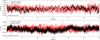 |
Fig. 1. Comparison of ten prior (red) and ten posterior (black) simulations in time-domain. Each line represents one independent realization of the respective type. The top panel shows sky model (i.e., CMB) simulations and the bottom panel shows correlated noise simulations. |
These intuitive differences translate directly into both qualitatively and quantitatively different ensemble properties for the resulting simulations, and correspondingly also into different resulting error estimates. As a real-world illustration of this, Fig. 2 shows slices through the empirical low-resolution polarization covariance matrix computed for each of the three Planck LFI frequency channels using three different generations of LFI simulations, namely (from left to right columns): Planck 2018 (Planck Collaboration II 2020), Planck PR4 (Planck Collaboration Int. LVII 2020), and BEYONDPLANCK (BeyondPlanck Collaboration 2023). Row sections show results for the 30, 44, and 70 GHz channels, respectively, and within each section the two rows show the QQ and UQ segments of the full matrix, sliced through Stokes Q pixel number 100, marked in gray in the upper right quadrant. Each covariance matrix is computed by first downgrading each simulation to a HEALPix4 (Górski et al. 2005) resolution of Nside = 8, and averaging the outer product over all available realizations; we refer to Basyrov et al. (2023), Colombo et al. (2023) for further details. Effectively, these matrices visually summarize the map-space uncertainty estimates predicted by each simulation set.
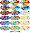 |
Fig. 2. Single column of the low-resolution 30 (top section), 44 (middle section), and 70 GHz (bottom section) frequency channel covariance matrix, as estimated from 300 LFI DPC FFP10 frequentist simulations (left column); from 300 PR4 prior simulations (middle column); and from 3200 BEYONDPLANCK posterior simulations (right column). The selected column corresponds to the Stokes Q pixel number 100 marked in gray, which is located in the top right quadrant. All covariance matrices are constructed at Nside = 8. Note: the Planck PR4 30 GHz covariance slice has been divided by a factor of 5 and thus it is even stronger than the color scale naively implies. |
Starting with the Planck 2018 simulations, the most striking observation is that these empirical matrices are very noisy for all three frequency channels. This is partly a reflection of the fact that only 300 simulations were actually constructed, and this leads to a high Monte Carlo uncertainty. Specifically, the uncertainty due to a finite number of simulations scales as  , which suggests a 6% contribution for 300 simulations. However, because these simulations are prior-based, that number applies to all sources of variations between realizations, including white noise, instrumental effects, and sky-signal variations. Furthermore, the gains that were assumed when generating these simulations exhibited significantly less structure than the real observations. In summary, there are relatively little common structures between the various realizations, either from the astrophysical sky, the instrumental noise, or the gain, and the corresponding covariance structures are therefore weak. Visually speaking, perhaps the most notable feature is a positive correlation from correlated noise along the scanning direction that passes through the sliced pixel seen in the upper right quadrant, but these are significantly obscured by Monte Carlo uncertainties.
Proceeding to the Planck PR4 simulations summarized in the middle column, we now see very strong coherent structures for the 30 GHz channel, while the 44 and 70 GHz channels behave similarly to the 2018 case. The explanation for this qualitative difference is the Planck PR4 calibration algorithm; in this pipeline, the 30 GHz channel is calibrated independently without the use of supporting priors, while the 44 and 70 GHz channels are calibrated by using the 30 GHz channel as a polarized foreground prior. The net effect of this independent calibration procedure is a very high calibration uncertainty for the 30 GHz channel, and these couple directly to the true CMB dipole, which is kept fixed between all simulations. The result is the familiar large-scale pattern seen in this figure, which has been highlighted by several previous analyses as a particularly difficult mode to observe with Planck (e.g., Planck Collaboration II 2020; Gjerløw et al. 2023; Watts et al. 2023).
Turning to the BEYONDPLANCK simulations summarized in the right column, we now see coherent and signal-dominated structures across the full sky in all frequency channels. A part of this is simply due to more realizations than for the other two pipelines (in this case, 3200), but even more importantly, the simulations are now entirely data-driven. That is, they correspond to the black curves in Fig. 1, while the previous pipelines correspond to the red curves. In practice, this has two main effects. First, it implies that the total parameter volume that needs to be explored by Monte Carlo sampling is intrinsically smaller, simply because the posterior distribution does not include cosmic variance; the simulations only need to describe our instrument and universe – and not simply any instrument and universe, and this is a much smaller sub-set. Second, and even more importantly, the posterior simulations account naturally for non-linearity between the various parameters, and these are very often the dominant contributions in these distributions. As a concrete example, if the gain happens to scatter either high or low during a given time period, then the total uncertainty estimate will be particularly sensitive to the CMB dipole during the same time period, and it will excite a correlation structure in these plots that is intimately connected to the satellite scanning strategy. Thus, if one chooses a gain profile that is independent of other parameters, then those real uncertainties will not be properly accounted for in the simulation set: intuitively speaking, the hot and cold spots in the covariance matrices shown in Fig. 2 will either appear in the wrong places or be suppressed when averaging over independent realizations. In general, specifying the instrumental model at a sufficiently realistic level represents a real challenge for frequentist simulations, and great care is required in order to capture the full error budget. This task is considerably simplified in the Bayesian approach, as each instrumental parameter is defined directly from the data themselves.
4. Simulation specification
Returning to the data model summary in Sect. 2, we note that the Commander3 code described by Galloway et al. (2023a), and used by the BEYONDPLANCK project to perform Bayesian end-to-end analysis of the Planck LFI data, is able to produce both prior and posterior simulations essentially without modifications; the only question is whether the parameters used to generate the TOD, ω, are drawn from the posterior distribution, or whether they are selected from a data-independent hyper-distribution. Choosing which type of simulations to generate is thus only a matter of selecting proper initialization values in the Commander3 parameter file.
In this paper, we demonstrate the frequentist mode of operation by generating a set of classical frequentist simulations with Commander3, and we then use these to validate the novel low-level processing algorithms introduced by Keihänen et al. (2023), Ihle et al. (2023), Gjerløw et al. (2023) for mapmaking, correlated noise estimation, and gain estimation, respectively.
We note that the original BEYONDPLANCK analysis required 670 000 CPU-hours to generate 4000 full Gibbs samples for the full LFI dataset, which took about three months of runtime to complete. In the current paper, we are primarily interested in validating the low-level algorithms themselves, and we therefore chose to consider only one year of 30 GHz observations in the following (corresponding to about 10 000 Planck pointing periods (PIDs), each lasting for about one hour; Planck Collaboration I 2014), rather than the full LFI dataset, and this reduces the computational cost from 169 to 2.5 CPU-hours per Gibbs sample (Galloway et al. 2023a). As a result, we are able to produce individual chains with 10 000 samples within a matter of days, rather than months or years, which is useful for convergence analyses. This also reduces the total volume of the TOD themselves (not including pointing, flags, etc.) from 638 GB to 22 GB, and the simulations may therefore be run on a much broader range of hardware. In fact, subsets of the following simulations have been produced on more than ten different computing systems all over the world, using both AMD and Intel processors (e.g., Intel E5-2697v2 2.7 GHz, Intel Xeon E5-2698 2.3 GHz, Intel Xeon W-2255 3.7 GHz, AMD Ryzen 9 3950X 2.2 GHz), with between 128 GB and 1.5 TB RAM per node, and using both Intel and GNU compilers5.
Given that we will only consider low-level processing of the 30 GHz channel, we simplify the data model in Eq. (1) to

Here, we only included one single sky component, namely the CMB, and we ignored sub-dominant effects such as far sidelobe corrections, 1 Hz electronic spikes, etc. As such, this configuration provides a test of the gain, noise estimation, and mapmaking parts of the full algorithm, but neglecting the component separation or cosmological parameter estimation.
The CMB sky realizations used in the following analysis are drawn from the best-fit Planck 2018 ΛCDM model (Planck Collaboration V 2020), using the HEALPix6 (Górski et al. 2005) synfast utility. All instrumental parameters are drawn from different realizations of the BEYONDPLANCK ensemble presented in BeyondPlanck Collaboration (2023) and these are taken as true input values in the following.
For the noise terms, we drew a random Gaussian realization of  with the noise PSD model given in Eq. (2). This was done independently for each Planck pointing ID (PID) and the noise PSD parameters thus vary over time with the same structure as the real observations.
5. Validation of low-level processing algorithms
To validate the noise and gain estimation and mapmaking steps in Commander3, we analyzed the prior simulations described above with the same Bayesian framework as used for the main BEYONDPLANCK processing and we compared the output marginal posterior distributions with the known true inputs. To quantify both biases and the accuracy of the uncertainty estimates, we adopted the following normalized residual,
where μω and σω are the posterior mean and standard deviation for parameter ω. For a truly Gaussian posterior distribution with no bias and perfect uncertainty estimation, this quantity should be distributed according to a standard normal distribution with zero mean and unit variance, N(0, 1), while a non-zero value of δ indicates a bias measured in units of σ. It is of course important to note that the full data model in Eq. (1) is highly non-linear due to the presence of the gain. Therefore, the deviations from N(0, 1) at some level are fully expected, in particular for signal-dominated quantities. Still, we find that δ serves as a useful quality monitor.
Unless otherwise noted, the main results presented in the following are derived from a single Markov chain comprising 10 000 samples. Where it proves useful for convergence and mixing assessment, we also used shorter and independent chains, typically with 1000 samples in each chain.
5.1. Markov auto-correlations
We are also interested in studying the statistical properties of individual Markov chains in terms of correlation lengths, degeneracies, and convergence. We define the Markov chain auto-correlation for a given chain as:
where i denotes Gibbs sample number, and Δ is a chain lag parameter that denotes the sample separation.
Figure 3 shows the auto-correlation for a typical set of parameters. The top four panels display: (1) a single CMB map pixel (in T, Q, and U); (2) a single correlated noise map pixel (in T, Q, and U); (3) the CMB temperature quadrupole moment, a2, 0; and (4) the gain for a single PID. These all have relatively short correlation lengths, which indicates that we are likely to produce robust results for these parameters.
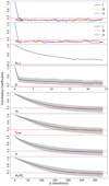 |
Fig. 3. Auto-correlation function, ρ, for selected parameters in the model, as estimated from a single chain with 10 000 samples. From top to bottom, the various panels show (1) one pixel value of the CMB component map mCMB; (2) one pixel of the correlated noise map mncorr; (3) the temperature quadrupole moment, a2, 0; (4) the PID-averaged total gain g; and (5)–(8) the PID-averaged noise PSD parameters σ0, fknee, α, and Ap/σ0. In panels with multiple lines, the various colors show Stokes T, Q, and U parameters. In panels with gray bands, the black line shows results averaged over all PIDs, and the band shows the 1σ variation among PIDs. The dashed red line marks a correlation coefficient of 0.1, which is used to define the typical correlation length of each parameter. |
In contrast, the parameters in the bottom four panels have very long correlation lengths, and these correspond to the four correlated noise PSD parameters within a single PID; σ0, fknee, α, and Ap/σ0. As discussed by Ihle et al. (2023), the introduction of the log-normal noise term greatly increases degeneracies and correlations among these parameters as compared to a standard 1/f noise profile, and this makes a proper estimation of these parameters much more expensive. However, it is also important to note that this is only a challenge regarding the estimation of the individual noise PSD parameters. In fact, the full PSD as a function of frequency, Pn(f), is insensitive to these degeneracies and that function is the only thing that is actually propagated to the rest of the system. This explains why the long correlations seen in the lower half of the plot do not excite long correlations also among the (far more important) parameters in the top half of the plot.
In fact, the single most important parameter in the entire system is the CMB map, shown in the first (for individual pixels) and third (for the quadrupole moment, a2, 0) panels. Indeed, the correlation length is very short or even non-existent for single pixels. This is primarily due to the fact that this map is strongly dominated by white noise on a single-pixel scale for the setup we consider here. As seen in the third panel, the same does not hold true for the quadrupole moment, in which case the correlation is in fact higher than 0.3 at a lag of Δ = 25. The main driver for this is the gain, as shown in the fourth panel. While the gain is dominated by white noise on short time-scales (as seen by the quick drop-off between lags of 1 and 2), there is a slow drift at higher lags. This is caused by a partial degeneracy between the CMB map (which acts as a calibration source in this framework, anchored by the orbital dipole) and the overall gain. In the real BEYONDPLANCK analysis, this degeneracy is mitigated to a large extent by analyzing all LFI channels jointly, and also by including WMAP observations to break important low-ℓ polarization degeneracies (Gjerløw et al. 2023; Basyrov et al. 2023). Still, even with those additions, there are important long-term drifts in the largest CMB temperature scales, and these have non-negligible consequences for the statistical significance of low-ℓ CMB anomalies (Colombo et al. 2023).
5.2. Posterior distribution overview
Next, to build the intuition regarding the full set of recovered parameters, we show in Fig. 4 the marginal 1D and 2D posterior distributions for a small set of parameters for two different PIDs. In each panel, the true input values are shown as dashed lines. The bottom triangle (blue) show posterior results for one well-behaved PID with good goodness-of-fit statistics, while the top triangle (orange) shows a less well-behaved case in which the true input values are at the edge of recovered distributions. Together, these two cases represent the majority of all PIDs in terms of overall behaviour.
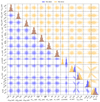 |
Fig. 4. Recovered posterior distributions for a selected set of parameters from two PIDs and detectors. The contours indicate 68 and 95% confidence regions, while the dashed lines (in the respective color of the contours) show the true input value of each of the PIDs. The contours below (blue) and above (orange) the diagonal correspond to PIDs 3003 and 5515, respectively. From left to right along the horizontal axis, columns show (1)–(3) one arbitrary CMB map pixel in Stokes I, Q, and U; (4)–(6) correlated noise for the same pixel and Stokes parameters; (7) the CMB intensity quadrupole amplitude a2, 0; (8) gain g; and (9)–(12) the four correlated noise parameters, ξn = {σ0, fknee, α, Ap}. Note: the 1D histograms of the first seven parameters are completely overlapping since these parameters are independent of PID. |
Overall, the true input parameters are recovered reasonably well in most cases. One of the parameters that is not as well recovered is the white noise amplitude, σ0. This parameter is a special case due to the sampling algorithm currently used in the BEYONDPLANCK pipeline. As described by Ihle et al. (2023), σ0 is currently determined as the standard deviation of all pairwise differences between neighboring time samples divided by  . While this is a commonly used technique in radio astronomy to derive an estimate of the white noise that is highly robust against unmodeled systematic errors, it does not correspond to a proper sample from the true conditional distribution P(σ0 ∣ d, g, …). In particular, this approach underestimates the true fluctuations of σ0, which in turn results in the overall uncertainties being slightly underestimated. This is one of several examples in the pipeline in which robustness to systematic effects comes at a cost of statistical rigor. At the same time, it is important to note that the absolute white noise level is in general very well determined in these data (Ihle et al. 2023) and a slight under-estimation of the uncertainty in σ0 has little practical impact on other parameters in the model.
Looking more broadly at the 2D distributions in this figure, we see that the parameters are split naturally into two groups, defined by the short and long correlation lengths discussed above. That is to say, the CMB, correlation noise, and gain parameters generally exhibit more symmetric distributions than the noise PSD distributions, which are highly correlated and non-Gaussian. Once again, this reflects the internal degeneracies among the noise PSD parameters.
To further illustrate the impact of the slow convergence rate for several of these parameters, Fig. 5 shows four partial chains, each with only 1000 samples, for a sub-set of these parameters. Once again, we see that the input values are reasonably well recovered for most cases, but each colored subdistribution only covers a modest part of the full posterior volume.
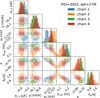 |
Fig. 5. Comparison of partial posteriors distributions from multiple short chains for the quadrupole amplitude, a2, 0, the gain, g, white noise level, σ0, knee frequency, fknee, correlated noise spectral index α, and log-normal noise amplitude, Ap. Each chain consists of 1000 samples. The posterior contours only span the range of the underlying samples, thereby making some of them appear open. |
5.3. Gain validation
In going into greater detail with respect to individual parameters, we show in Fig. 6 a subset of the estimated gain as a function of Gibbs iteration for four selected PIDs, that is: one for each radiometer. The red lines show the true input values. Here, we visually observe the same behavior as discussed above; on short time scales, these trace plots are dominated by random fluctuations, while on long time-scales, there are still obvious significant drifts.
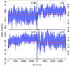 |
Fig. 6. Trace plots of gain values as a function of chain iteration (blue) compared to their input values (red) for selected PIDs, in order from left to right: 349, 9847, 4298, and 1993. |
Figure 7 compares the estimated gain (blue bands) with the known input (red curves) as a function of PID. The width of the blue bands indicates the ±1σ confidence region. At least at a visual level, the two curves agree well, without any obvious evidence of systematic biases, and the uncertainties appear reasonable. These observations are made more quantitative in Fig. 8, which shows histograms of normalized residuals, δg, over all PIDs. Red lines indicate the standard Gaussian N(0, 1) reference distribution. Once again, we see that the reconstruction appears good, as the nominal bias is (at most) 0.36σ, and the maximum posterior width is 1.36σ. From the shape of the histograms, it is also clear that a significant fraction of these variations is due to the Monte Carlo sample variance from the long gain-correlation lengths. Once again, we note that such deviations will decrease as the number of frequency bands included in the analysis increases, since the Solar CMB dipole, which is the main calibrator, will be much better constrained with more observations. The actual gain-correlation lengths found for the real BEYONDPLANCK analysis are shown by Gjerløw et al. (2023) and they are notably shorter than those of this reduced simulation.
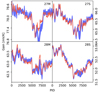 |
Fig. 7. Input gain values (red) over-plotted on the output gain values (blue). The width of the blue line indicates the sample standard deviation of the PID in question. |
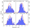 |
Fig. 8. Aggregate standard deviation normalized differences between the gain sample mean and the input gain values. For each PID t and detector i we calculate |
5.4. Correlated noise posterior validation
Next, we turn to the correlated noise component, and we start with the specific noise realization, ncorr (the correlated noise PSD parameters is discussed separately in Sect. 5.6). To simplify the visualization, we binned the correlated noise TOD into a sky map, as illustrated in Fig. 9. The top-left panel shows the true input correlated noise map (temperature component only), while the top-right panel shows the corresponding posterior mean (output) map. The bottom-left panel shows the posterior standard deviation per pixel and the bottom-right panel shows the normalized residual, δcorr.
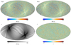 |
Fig. 9. Pixel space comparison of reconstructed correlated noise maps in temperature. Top left: true input realization. Top right: estimated posterior mean (output) map. Bottom left: estimated posterior standard deviation map. Bottom right: normalized residual in units of standard deviations. |
A visual inspection of the simulation input and posterior mean correlated noise maps indicates no obvious differences. In fact, the normalized residual map in the bottom right panel of Fig. 9 appears fully consistent with white noise. Once again, this observation is quantified more accurately in Fig. 10, where we compare the histogram of δcorr over all pixels with the usual N(0, 1) distribution for each of the three Stokes parameters. In each case, the agreement is excellent.
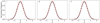 |
Fig. 10. Histograms of normalized correlated noise residuals, δ for each Stokes parameters (black distributions). For comparison, the dashed red line shows a standard N(0, 1) distribution. |
5.5. CMB map validation
Figures 11 and 12 show similar plots for the CMB sky map component. Once again, the normalized residual in the bottom right panel appears fully consistent with white noise over most of the sky. However, this time, we actually see a power excess in δCMB around the Ecliptic poles. These features correspond to regions of the sky that are particularly deeply observed by the Planck scanning strategy (Planck Collaboration I 2014). As a result of these deep measurements, the white noise in these regions is very low, and the total error budget per pixel is far more sensitive to the non-linear contributions in the system, in particular the coupling between the gain and the Solar dipole.
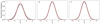 |
Fig. 12. Histograms of normalized CMB intensity residuals, δCMB for each Stokes parameters (black distributions). For comparison, the dashed red line shows a standard N(0, 1) distribution. |
This effect does of course not only apply to the Ecliptic “deep fields”, but to all signal-dominated map pixels at some level, and it therefore also applies to the full-sky CMB map in temperature. This statement is made more quantitative in the left panel of Fig. 12, where we see that the temperature histogram is very slightly wider than the reference N(0, 1) distribution. To be specific, the standard deviation of this distribution is about 1.15. At the same time, the mean of the distribution is consistent with zero, the non-linear couplings therefore do not introduce a bias, but only a higher variance. For the noise-dominated Stokes Q and U parameters, for which gain couplings are negligible on a per-pixel level, both distributions are perfectly consistent with N(0, 1).
Figure 13 shows Pearson’s correlation coefficients between the CMB and correlated noise components for three selected pixels. Two of the pixels, marked ‘1’ and ‘2’, are located along the same Planck scanning ring near the Ecliptic plane, where the Planck scanning strategy is particularly poor. The third pixel is located far away from these, and on a different scanning ring. Here, we see that correlations are very strong for Stokes parameters of the same type along the same ring, with correlation coefficients ranging between 0.5 and 0.8. These correlations are induced both by gain and correlated-noise fluctuations, which are tightly associated with the Planck scanning rings. Stokes parameters of different types (e.g. I and Q) are significantly less correlated, typically with anti-correlation coefficients of ρ ≲ −0.25. Correlations between widely separated pixels are practically negligible in the current simulation setup, although for the real analysis, this is no longer true due to additional couplings from, for instance, astrophysical foregrounds, bandpass corrections, and sidelobes (Galloway et al. 2023b; Svalheim et al. 2023a,b; Basyrov et al. 2023; Colombo et al. 2023; Andersen et al. 2023).
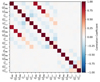 |
Fig. 13. Correlation matrix for selected pixel values of the CMB map, mCMB, and the correlated noise map, mncorr, for all three Stokes parameters I, Q, and U. Pixels 1 and 2 are selected to be neighboring pixels along the same Planck scanning ring and located near the Ecliptic plane, while pixel 3 is an arbitrarily selected pixel not spatially associated with the other two. |
5.6. Correlated noise PSD validation
Finally, we consider the noise PSD parameters, σ0, fknee, α, and Ap/σ0. As already noted, these are significantly harder to estimate individually than the previous parameters due to the strong correlation between the 1/f and log-normal terms in Eq. (2).
As usual, we plot the reduced residual, δ, for each parameter type in Fig. 14. In this case, we see that the posterior distributions are significantly wider than a standard Gaussian distribution, by as much as a factor of two. The distributions are also clearly non-Gaussian, with notable skewness and kurtosis. Both the excess variance and non-Gaussianity stem from the same degeneracies as discussed above and are partially due to intrinsic non-Gaussianities in the model, and partially due to incomplete Monte Carlo convergence and very long correlation lengths. On the other hand, the mean bias in these distribution is small and the estimated posterior distributions do provide a useful summary of each parameter individually.
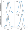 |
Fig. 14. Histograms of the noise parameters over all PIDs and 10 000 samples for radiometer 27M. We show the white noise level, σ0, knee frequency, fknee, correlated noise spectral index α, and log-normal noise amplitude, Ap. For reference, we show the standard normal distribution as a black dashed line. |
As mentioned above, however, other parameters in the model are not sensitive to individual ξn values, but only to the total noise PSD, Pcorr(f). This function is plotted in the top two panels of Fig. 15 for the same two PIDs and radiometers as shown in Fig. 4; the blue curves correspond to the aptly measured PID, while the orange curve corresponds to the PID with the marginal fit. Faint lines in the top two panels show individual Gibbs samples, corresponding to different combinations of ξn. By eye, the sampled values appear to span the true input reasonably well, although the orange line is on the lower edge of the estimated posterior distribution.
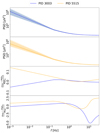 |
Fig. 15. Comparison of recovered correlated noise PSD in terms of the functional form, Pn(f). The top two panels show results for the same PIDs as in Fig. 4. Faint lines indicate individual Gibbs samples, while the dashed lines show the true input functions. The bottom two panels show the difference between the posterior mean function and the true input as a fraction of the latter and in units of the posterior rms, respectively. |
These visual observations are made more quantitative in the bottom two panels, where the third panel shows the fractional difference between the output and input PSD functions, and the fourth panel shows the same in units of standard deviation of the PSD across Gibbs samples, σ. For the well-behaved (blue) pixel, we see that the posterior mean matches the true input everywhere to within a few percent; in units of standard deviations, this is typically less than 2.5σ for most of the region, except at frequencies above 10 Hz, where the estimated standard deviation is very small due, and the underestimation of the uncertainty in σ0 becomes noticeable. For the less well-behaved case, the recovered PSD is within 2σ at all frequencies in units of standard deviations, or within 5 % otherwise. Overall, the PSD itself is recovered very well in both cases in absolute terms.
6. Conclusions
End-to-end time-ordered simulations play a key role in estimating both biases and uncertainties for current and future CMB experiments. To date, no other practical method has been able to account for the full and rich set of systematic errors that affect modern high-precision measurements.
As detailed in BeyondPlanck Collaboration (2023) and its companion papers, the BEYONDPLANCK project has implemented a new approach to end-to-end CMB analysis in which a global parametric model is fitted directly to the time-ordered data, allowing for joint estimation of instrumental, astrophysical, and cosmological parameters with true end-to-end error propagation. This approach relies strongly on a sampling algorithm called Gibbs sampling, which allows the user to draw joint samples from a complex posterior distribution. Each of these Gibbs samples correspond essentially to one end-to-end TOD simulation, similar to those produced by classical CMB simulation pipelines, such as the Planck full focalplane (FFP; Planck Collaboration XII 2016) simulations.
The fundamental difference between these two simulation pipelines lies in how to define the input parameters used to generate the simulation. In the BEYONDPLANCK approach, all parameters are constrained directly from the true data and correspond as such to samples drawn from the full joint posterior distribution. In contrast, traditional pipelines use parameters that are a mixture of data-constrained and data-independent parameters. Typical examples of the former include the CMB Solar dipole and Galactic foregrounds, while typical examples of the latter include CMB anisotropies and instrumental noise. In this paper, we call the two types of simulations for posterior- or prior-based, respectively, indicating whether (or not) they are conditioned on true data.
The difference between these two types of simulations has direct real-world consequences for what applications each simulation type is suitable for. As was first argued by Basyrov et al. (2023), this may be intuitively understood through the following line of reasoning. Supposing we are looking to construct a new end-to-end simulation for a given experiment. Among the first decisions that needs to be made concerns the CMB Solar dipole, answering the question of whether this should correspond to the true dipole or whether it should have a random amplitude and direction. If it is chosen randomly, then the hot and cold spots in the correlation matrices shown in Fig. 2 in this paper will appear at random positions on the sky, and eventually be washed out in an ensemble average. In practice, all current pipelines adopt the true CMB Solar dipole as an input. The next question is related to the type of Galactic model that should be used. Once again, if this is selected randomly, then the Galactic plane will move around on the sky from realization to realization. In practice, all current pipelines adopt a model of the true Galactic signal as an input.
The third question considers which CMB anisotropies should be used. At this point, all pipelines prior to BEYONDPLANCK have in fact adopted random CMB skies drawn from a theoretical ΛCDM model. This has two main effects: on the one hand, in the same way that randomizing the CMB dipole signal would average out any coherent correlations between the sky signal and the gain, randomizing the CMB anisotropies also average out, and non-linear correlations between these structures and the instrumental parameters are not accounted for. On the other hand, the resulting simulations do actually include so-called cosmic variance, that is, for the scatter between individual CMB realizations.
Finally, the same question apply to all the instrumental parameters, perhaps most notably correlated noise and gain fluctuations: we ask whether these ought to be constrained by the real data, or whether they should be drawn randomly from a laboratory-determined hyper-distribution.
It is important to stress that none of these four questions have a “right” or “wrong” answer. However, whatever choice is made, it will have direct consequences for what correlation structures appear among the resulting simulations and, thus, also for the sorts of applications they are suitable for. In particular, if the primary application is traditional frequentist model testing (e.g., asking whether the CMB sky is Gaussian and isotropic), then it is critical to account for cosmic variance among the CMB realizations. For those applications, we must choose data-independent CMB inputs in order to capture the full uncertainties and the appropriate choice are frequentist data-independent simulation inputs.
If, on the other hand, the main application is traditional parameter estimation, for instance, to constrain the ΛCDM model, then it is key to properly estimate the total CMB uncertainty per-pixel on the sky. In this case, it is critical to properly model all non-linear couplings between the actual sky signal, the true gain, the true correlated noise, and so on. In this case, the appropriate choices are posterior-based data-dependent simulation inputs.
In this paper, we note that the novel Commander3 software is able to produce both prior and posterior simulations simply by adjusting the inputs that are used to initialize the code. While the posterior simulation process has been described in detail in most of the BEYONDPLANCK companion papers, in the current paper, we present a first application of the frequentist mode of operation by producing a data-independent time-ordered simulation corresponding to one year of 30 GHz data. We we then used this to validate three important low-level steps in the full BEYONDPLANCK Gibbs samples, namely, gain estimation, correlated noise estimation, and mapmaking. In doing so, we find that the recovered posterior distribution matches the true input parameters well.
Acknowledgments
We thank Prof. Pedro Ferreira and Dr. Charles Lawrence for very useful suggestions, comments and discussions. We also thank the entire Planck and WMAP teams for invaluable support and discussions, and for their dedicated efforts through several decades without which this work would not be possible. This research has partially been carried out within the master- and PhD-level course “AST9240 – Cosmological component separation” at the University of Oslo, and support for this has been provided by the Research Council of Norway through grant agreement no. 274990. The BeyondPlanck Collaboration has received funding from the European Union’s Horizon 2020 research and innovation programme under grant agreement numbers 776282, 772253, and 819478. In addition, the collaboration acknowledges support from ESA; ASI, CNR, and INAF (Italy); NASA and DoE (USA); Tekes, AoF, and CSC (Finland); RCN (Norway); ERC and PRACE (EU). L. T. Hergt was supported by a UBC Killam Postdoctoral Research Fellowship. The work of Tamaki Murokoshi was supported by MEXT KAKENHI Grant Number 18H05539 and the Graduate Program on Physics for the Universe (GP-PU), Tohoku University. Part of the work by F. Rahman was carried out using the Nova and Coolstar clusters at the Indian Institute of Astrophysics, Bangalore. The work of K. S. F. Fornazier, G. A. Hoerning, A. Marins and F. B. Abdalla was developed in the Brazilian cluster SDumont and was supported by São Paulo Research Foundation (FAPESP) grant 2014/07885-0, National Council for Scientific and Technological (CNPQ), Coordination for the Improvement of Higher Education Personnel (CAPES) and University of São Paulo (USP). Some of the results in this paper have been derived using the healpy (Zonca et al. 2019) and HEALPix (Górski et al. 2005) packages. This work made use of Astropy (http://www.astropy.org) (Astropy Collaboration 2013, 2018, 2022).
References
- Andersen, K. J., Herman, D., Aurlien, R., et al. 2023, A&A, 675, A13 (BeyondPlanck SI) [NASA ADS] [CrossRef] [EDP Sciences] [Google Scholar]
- Astropy Collaboration (Robitaille, T. P., et al.) 2013, A&A, 558, A33 [NASA ADS] [CrossRef] [EDP Sciences] [Google Scholar]
- Astropy Collaboration (Price-Whelan, A. M., et al.) 2018, AJ, 156, 123 [Google Scholar]
- Astropy Collaboration (Price-Whelan, A. M., et al.) 2022, ApJ, 935, 167 [NASA ADS] [CrossRef] [Google Scholar]
- Basyrov, A., Suur-Uski, A.-S., Colombo, L. P. L., et al. 2023, A&A, 675, A10 (BeyondPlanck SI) [NASA ADS] [CrossRef] [EDP Sciences] [Google Scholar]
- Bennett, C. L., Larson, D., Weiland, J. L., et al. 2013, ApJS, 208, 20 [Google Scholar]
- BeyondPlanck Collaboration (Andersen, K. J., et al.) 2023, A&A, 675, A1 (BeyondPlanck SI) [Google Scholar]
- Colombo, L. P. L., Eskilt, J. R., Paradiso, S., et al. 2023, A&A, 675, A11 (BeyondPlanck SI) [NASA ADS] [CrossRef] [EDP Sciences] [Google Scholar]
- Eriksen, H. K., O’Dwyer, I. J., Jewell, J. B., et al. 2004, ApJS, 155, 227 [Google Scholar]
- Galloway, M., Andersen, K. J., Aurlien, R., et al. 2023a, A&A, 675, A3 (BeyondPlanck SI) [NASA ADS] [CrossRef] [EDP Sciences] [Google Scholar]
- Galloway, M., Reinecke, M., Andersen, K. J., et al. 2023b, A&A, 675, A8 (BeyondPlanck SI) [NASA ADS] [CrossRef] [EDP Sciences] [Google Scholar]
- Gelman, A., Vehtari, A., Simpson, D., et al. 2020, ArXiv e-prints [arXiv:2011.01808] [Google Scholar]
- Gerakakis, S., Brilenkov, M., Ieronymaki, M., et al. 2023, OJA, 6, 10 [NASA ADS] [Google Scholar]
- Gjerløw, E., Ihle, H. T., Galeotta, S., et al. 2023, A&A, 675, A7 (BeyondPlanck SI) [NASA ADS] [CrossRef] [EDP Sciences] [Google Scholar]
- Górski, K. M., Hivon, E., Banday, A. J., et al. 2005, ApJ, 622, 759 [Google Scholar]
- Ihle, H. T., Bersanelli, M., Franceschet, C., et al. 2023, A&A, 675, A6 (BeyondPlanck SI) [NASA ADS] [CrossRef] [EDP Sciences] [Google Scholar]
- Keihänen, E., Suur-Uski, A.-S., Andersen, K. J., et al. 2023, A&A, 675, A2 (BeyondPlanck SI) [NASA ADS] [CrossRef] [EDP Sciences] [Google Scholar]
- LiteBIRD Collaboration (Allys, E., et al.) 2023, PTEP, 2023, 042F01 [Google Scholar]
- Planck Collaboration I. 2014, A&A, 571, A1 [NASA ADS] [CrossRef] [EDP Sciences] [Google Scholar]
- Planck Collaboration I. 2016, A&A, 594, A1 [NASA ADS] [CrossRef] [EDP Sciences] [Google Scholar]
- Planck Collaboration XII. 2016, A&A, 594, A12 [NASA ADS] [CrossRef] [EDP Sciences] [Google Scholar]
- Planck Collaboration I. 2020, A&A, 641, A1 [NASA ADS] [CrossRef] [EDP Sciences] [Google Scholar]
- Planck Collaboration II. 2020, A&A, 641, A2 [NASA ADS] [CrossRef] [EDP Sciences] [Google Scholar]
- Planck Collaboration V. 2020, A&A, 641, A5 [NASA ADS] [CrossRef] [EDP Sciences] [Google Scholar]
- Planck Collaboration Int. LVII., 2020, A&A, 643, A42 [NASA ADS] [CrossRef] [EDP Sciences] [Google Scholar]
- Reinecke, M., Dolag, K., Hell, R., Bartelmann, M., & Ensslin, T. A. 2015, Astrophysics Source Code Library [record ascl:1505.032] [Google Scholar]
- Svalheim, T. L., Zonca, A., Andersen, K. J., et al. 2023a, A&A, 675, A9 (BeyondPlanck SI) [NASA ADS] [CrossRef] [EDP Sciences] [Google Scholar]
- Svalheim, T. L., Andersen, K. J., Aurlien, R., et al. 2023b, A&A, 675, A14 (BeyondPlanck SI) [NASA ADS] [CrossRef] [EDP Sciences] [Google Scholar]
- Wandelt, B. D., Larson, D. L., & Lakshminarayanan, A. 2004, Phys. Rev. D, 70, 083511 [Google Scholar]
- Watts, D. J., Galloway, M., Ihle, H. T., et al. 2023, A&A, 675, A16 (BeyondPlanck SI) [NASA ADS] [CrossRef] [EDP Sciences] [Google Scholar]
- Zonca, A., Singer, L., Lenz, D., et al. 2019, J. Open Source Softw., 4, 1298 [Google Scholar]
All Figures
|
Fig. 1. Comparison of ten prior (red) and ten posterior (black) simulations in time-domain. Each line represents one independent realization of the respective type. The top panel shows sky model (i.e., CMB) simulations and the bottom panel shows correlated noise simulations. |
| In the text | |
|
Fig. 2. Single column of the low-resolution 30 (top section), 44 (middle section), and 70 GHz (bottom section) frequency channel covariance matrix, as estimated from 300 LFI DPC FFP10 frequentist simulations (left column); from 300 PR4 prior simulations (middle column); and from 3200 BEYONDPLANCK posterior simulations (right column). The selected column corresponds to the Stokes Q pixel number 100 marked in gray, which is located in the top right quadrant. All covariance matrices are constructed at Nside = 8. Note: the Planck PR4 30 GHz covariance slice has been divided by a factor of 5 and thus it is even stronger than the color scale naively implies. |
| In the text | |
|
Fig. 3. Auto-correlation function, ρ, for selected parameters in the model, as estimated from a single chain with 10 000 samples. From top to bottom, the various panels show (1) one pixel value of the CMB component map mCMB; (2) one pixel of the correlated noise map mncorr; (3) the temperature quadrupole moment, a2, 0; (4) the PID-averaged total gain g; and (5)–(8) the PID-averaged noise PSD parameters σ0, fknee, α, and Ap/σ0. In panels with multiple lines, the various colors show Stokes T, Q, and U parameters. In panels with gray bands, the black line shows results averaged over all PIDs, and the band shows the 1σ variation among PIDs. The dashed red line marks a correlation coefficient of 0.1, which is used to define the typical correlation length of each parameter. |
| In the text | |
|
Fig. 4. Recovered posterior distributions for a selected set of parameters from two PIDs and detectors. The contours indicate 68 and 95% confidence regions, while the dashed lines (in the respective color of the contours) show the true input value of each of the PIDs. The contours below (blue) and above (orange) the diagonal correspond to PIDs 3003 and 5515, respectively. From left to right along the horizontal axis, columns show (1)–(3) one arbitrary CMB map pixel in Stokes I, Q, and U; (4)–(6) correlated noise for the same pixel and Stokes parameters; (7) the CMB intensity quadrupole amplitude a2, 0; (8) gain g; and (9)–(12) the four correlated noise parameters, ξn = {σ0, fknee, α, Ap}. Note: the 1D histograms of the first seven parameters are completely overlapping since these parameters are independent of PID. |
| In the text | |
|
Fig. 5. Comparison of partial posteriors distributions from multiple short chains for the quadrupole amplitude, a2, 0, the gain, g, white noise level, σ0, knee frequency, fknee, correlated noise spectral index α, and log-normal noise amplitude, Ap. Each chain consists of 1000 samples. The posterior contours only span the range of the underlying samples, thereby making some of them appear open. |
| In the text | |
|
Fig. 6. Trace plots of gain values as a function of chain iteration (blue) compared to their input values (red) for selected PIDs, in order from left to right: 349, 9847, 4298, and 1993. |
| In the text | |
|
Fig. 7. Input gain values (red) over-plotted on the output gain values (blue). The width of the blue line indicates the sample standard deviation of the PID in question. |
| In the text | |
|
Fig. 8. Aggregate standard deviation normalized differences between the gain sample mean and the input gain values. For each PID t and detector i we calculate |
| In the text | |
|
Fig. 9. Pixel space comparison of reconstructed correlated noise maps in temperature. Top left: true input realization. Top right: estimated posterior mean (output) map. Bottom left: estimated posterior standard deviation map. Bottom right: normalized residual in units of standard deviations. |
| In the text | |
|
Fig. 10. Histograms of normalized correlated noise residuals, δ for each Stokes parameters (black distributions). For comparison, the dashed red line shows a standard N(0, 1) distribution. |
| In the text | |
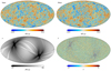 |
Fig. 11. Same as Fig. 9, but for the CMB intensity component. |
| In the text | |
|
Fig. 12. Histograms of normalized CMB intensity residuals, δCMB for each Stokes parameters (black distributions). For comparison, the dashed red line shows a standard N(0, 1) distribution. |
| In the text | |
|
Fig. 13. Correlation matrix for selected pixel values of the CMB map, mCMB, and the correlated noise map, mncorr, for all three Stokes parameters I, Q, and U. Pixels 1 and 2 are selected to be neighboring pixels along the same Planck scanning ring and located near the Ecliptic plane, while pixel 3 is an arbitrarily selected pixel not spatially associated with the other two. |
| In the text | |
|
Fig. 14. Histograms of the noise parameters over all PIDs and 10 000 samples for radiometer 27M. We show the white noise level, σ0, knee frequency, fknee, correlated noise spectral index α, and log-normal noise amplitude, Ap. For reference, we show the standard normal distribution as a black dashed line. |
| In the text | |
|
Fig. 15. Comparison of recovered correlated noise PSD in terms of the functional form, Pn(f). The top two panels show results for the same PIDs as in Fig. 4. Faint lines indicate individual Gibbs samples, while the dashed lines show the true input functions. The bottom two panels show the difference between the posterior mean function and the true input as a fraction of the latter and in units of the posterior rms, respectively. |
| In the text | |
Current usage metrics show cumulative count of Article Views (full-text article views including HTML views, PDF and ePub downloads, according to the available data) and Abstracts Views on Vision4Press platform.
Data correspond to usage on the plateform after 2015. The current usage metrics is available 48-96 hours after online publication and is updated daily on week days.
Initial download of the metrics may take a while.