| Issue |
A&A
Volume 675, July 2023
BeyondPlanck: end-to-end Bayesian analysis of Planck LFI
|
|
|---|---|---|
| Article Number | A3 | |
| Number of page(s) | 17 | |
| Section | Numerical methods and codes | |
| DOI | https://doi.org/10.1051/0004-6361/202243137 | |
| Published online | 28 June 2023 | |
BEYONDPLANCK
III. Commander3
1
Institute of Theoretical Astrophysics, University of Oslo, Blindern, Oslo, Norway
e-mail: mathew.galloway@astro.uio.no
2
Dipartimento di Fisica, Università degli Studi di Milano, Via Celoria, 16, Milano, Italy
3
INAF-IASF Milano, Via E. Bassini 15, Milano, Italy
4
INFN, Sezione di Milano, Via Celoria 16, Milano, Italy
5
INAF – Osservatorio Astronomico di Trieste, Via G. B. Tiepolo 11, Trieste, Italy
6
Planetek Hellas, Leoforos Kifisias 44, Marousi, 151 25
Greece
7
Department of Astrophysical Sciences, Princeton University, Princeton, NJ, 08544
USA
8
Jet Propulsion Laboratory, California Institute of Technology, 4800 Oak Grove Drive, Pasadena, CA, USA
9
Department of Physics, University of Helsinki, Gustaf Hällströmin katu 2, Helsinki, Finland
10
Helsinki Institute of Physics, University of Helsinki, Gustaf Hällströmin katu 2, Helsinki, Finland
11
Computational Cosmology Center, Lawrence Berkeley National Laboratory, Berkeley, CA, USA
12
Haverford College Astronomy Department, 370 Lancaster Avenue, Haverford, PA, USA
13
Max-Planck-Institut für Astrophysik, Karl-Schwarzschild-Str. 1, 85741 Garching, Germany
14
Dipartimento di Fisica, Università degli Studi di Trieste, Via A. Valerio 2, Trieste, Italy
Received:
17
January
2022
Accepted:
25
February
2022
We describe the computational infrastructure for end-to-end Bayesian cosmic microwave background (CMB) analysis implemented by the BeyondPlanck Collaboration. The code is called Commander3. It provides a statistically consistent framework for global analysis of CMB and microwave observations and may be useful for a wide range of legacy, current, and future experiments. The paper has three main goals. Firstly, we provide a high-level overview of the existing code base, aiming to guide readers who wish to extend and adapt the code according to their own needs or re-implement it from scratch in a different programming language. Secondly, we discuss some critical computational challenges that arise within any global CMB analysis framework, for instance in-memory compression of time-ordered data, fast Fourier transform optimization, and parallelization and load-balancing. Thirdly, we quantify the CPU and RAM requirements for the current BEYONDPLANCK analysis, finding that a total of 1.5 TB of RAM is required for efficient analysis and that the total cost of a full Gibbs sample for LFI is 170 CPU-hrs, including both low-level processing and high-level component separation, which is well within the capabilities of current low-cost computing facilities. The existing code base is made publicly available under a GNU General Public Library (GPL) license.
Key words: methods: data analysis / cosmic background radiation / methods: numerical
© The Authors 2023
 Open Access article, published by EDP Sciences, under the terms of the Creative Commons Attribution License (https://creativecommons.org/licenses/by/4.0), which permits unrestricted use, distribution, and reproduction in any medium, provided the original work is properly cited.
This article is published in open access under the Subscribe to Open model. Subscribe to A&A to support open access publication.
1. Introduction
The aim of the BEYONDPLANCK project (BeyondPlanck Collaboration 2023) is to build an end-to-end Bayesian cosmic microwave background (CMB) analysis pipeline that constrains high-level products, such as astrophysical component maps and cosmological parameters, directly from raw uncalibrated time-ordered data and to apply this to the Planck Low-Frequency Instrument (LFI) data. This pipeline builds on the experience gained throughout the official Planck analysis period and seeks to translate this experience into reusable and computationally efficient computer code that can be used for end-to-end analysis of legacy, current, and future data sets. As a concrete and particularly important example, it will serve as the computational framework for the COSMOGLOBE1 effort, which aims to establish a consistent global model of the radio, microwave, and submillimeter sky through joint analysis of all available state-of-the-art data sets. This paper gives an overview of the BEYONDPLANCK computational infrastructure, and it details several computational techniques that allow the full exploration of the global posterior distribution in a timely manner.
Since the beginning of precision CMB cosmology, algorithm development has been a main focus of the community. For instance, during the early days of CMB analysis, many different approaches to mapmaking were explored. Projects such as COBE (Smoot et al. 1992; Bennett et al. 1996), MAX (White & Bunn 1995), Saskatoon (Tegmark et al. 1997) and Tenerife (Gutiérrez et al. 1996) used a wide variety of techniques, and optimality was not guaranteed. Soon, however, the community converged on Wiener filtering as the preferred technique (Tegmark 1997), which also allowed for the combination of multiple data sets into a single map (Xu et al. 2001).
By the time WMAP and its contemporaries were observing, the field had matured to the point that common tools were used between experiments. HEALPix2 (Gorski et al. 2005) became a defacto standard for pixelizing the sky, and many experiments began to use conjugate gradient (CG) mapmakers on a regular basis (e.g., Hinshaw et al. 2003). These ideas were refined during the analysis of Planck (Planck Collaboration I 2014, 2016, 2020), and since then those efforts have dominated the field. Many mapmaking tools that were developed for Planck have a strong influence on BEYONDPLANCK, including the MADAM destriper (Keihänen et al. 2005), the LevelS simulation codebase (Reinecke et al. 2006), the libsharp spherical harmonic transform library (Reinecke & Seljebotn 2013), and the Planck Data Release 4 analysis pipeline (Planck Collaboration Int. LVII 2020, often called NPIPE).
In parallel to these mapmaking developments, algorithms for component separation have also been gradually refined. Several different classes of methods have been explored and applied to a variety of experiments, including internal linear combination (ILC) methods such as WMAP ILC (Bennett et al. 2003; Eriksen et al. 2004a) and NILC (Delabrouille et al. 2009); template-based approaches such as SEVEM (Fernández-Cobos et al. 2012); spectral matching techniques such as SMICA (Cardoso et al. 2008); blind techniques such as GMCA (Bobin et al. 2007) or FastICA (Maino et al. 2002); and parametric Bayesian modeling techniques such as Commander (Eriksen et al. 2004b, 2008; Seljebotn et al. 2019). This flowering of options provided a range of complementary approaches that each gave new insights into the underlying statistical problem.
Simultaneously, there has been an immense development in computer hardware, increasing the amount of available CPU cycles and RAM by many orders of magnitude. As an example, the COBE analysis was in 1990 initially performed on VAXstation 3200 computers (Cheng 1992), which boasted 64 KB of RAM and a single 11 MHz processor. For comparison, the Planck FFP8 simulations (Planck Collaboration XII 2016) were in 2013 produced on a distributed Cray XC30 system with 133 824 cores, each with a clock speed of 2.4 GHz and 2 GB of RAM, at a total computational cost of 25 million CPU hours. While the evolution in CPU clock speed has largely stagnated during the last decade, the cost of RAM continues to decrease, and this has been exploited to improve the memory management efficiency in the current analysis: BEYONDPLANCK represents the first CMB analysis pipeline for which the full Planck LFI time-ordered data set may be stored in RAM on a single compute node, effectively alleviating the need for expensive disk and network communication operations during the analysis. As a result, the full computational cost of the current BEYONDPLANCK analysis is only 300 000 CPU hours, and, indeed, it is not entirely inconceivable that this analysis could be run on a laptop in the not too distant future.
The BEYONDPLANCK pipeline is a natural evolution and fusion of a wide range of these developments into a single integrated codebase. There are relatively few algorithmically novel features in this pipeline as such, but the BEYONDPLANCK pipeline primarily combines industry standard methods into one single framework. The computer code that realizes this is called Commander3, which is a direct generalization of Commander2. Whereas previous Commander versions focused primarily on high-level component separation and CMB power spectrum estimation applications (Eriksen et al. 2004b, 2008; Seljebotn et al. 2019), Commander3 also accounts for low-level time-ordered data processing and mapmaking. This integrated approach yields a level of performance and error propagation fidelity that we believe will be difficult to replicate with distributed methods that require intermediate human interaction. This paper describes the code implementation that is used to produce the results detailed in the BEYONDPLANCK paper suite and makes the results of that development available to the community.
The BEYONDPLANCK pipeline, documentation and data are all available through the project webpage3. In addition to the actual Commander3 source code4, several utilties are also provided that facilitate easy use of the codes by others in the community, for instance for downloading data and compiling and running the codes. Documentation is also available5. The entire project is available under the GNU General Public License (GPL). Further details regarding these aspects are available in Gerakakis et al. (2023).
2. Bayesian CMB analysis, Gibbs sampling, and code design
The main goals of the current paper are, firstly, to provide sufficient intuition regarding the Commander3 source code to allow external users to navigate and modify it themselves, and, secondly, to present various computational techniques that are used to optimize the calculations. To set the context of this work, we begin by briefly summarizing the main computational ideas behind this approach.
2.1. The BEYONDPLANCK data model and Gibbs chain
As described by BeyondPlanck Collaboration (2023), Commander3 is the first end-to-end Bayesian analysis framework for CMB experiments, implementing full Monte Carlo Markov chain (MCMC) exploration of a global posterior distribution. The most important component in this framework is an explicit parametric model. The current BEYONDPLANCK project primarily focuses on the Planck LFI measurements (Planck Collaboration I 2020; Planck Collaboration II 2020), and for this data set we find that the following model represents a good description of the available measurements (BeyondPlanck Collaboration 2023),
![$$ \begin{aligned} d_{j,t} =&g_{j,t}\mathsf{P }_{tp,j}\left[\mathsf{B }^{\mathrm{symm} }_{pp^\prime ,j}\sum _{c} \mathsf{M }_{cj}(\beta _{p^\prime }, \Delta _{\mathrm{bp} }^{j})a^c_{p^\prime } + \mathsf{B }^{\mathrm{asymm} }_{pp^\prime ,j}\left(s^{\mathrm{orb} }_{j,t} + s^{\mathrm{fsl} }_{j,t}\right)\right]\nonumber \\&+ s^\mathrm{1\,hz }_{j,t} + n^{\mathrm{corr} }_{j,t} + n^{\mathrm{w} }_{j,t}. \end{aligned} $$](/articles/aa/full_html/2023/07/aa43137-22/aa43137-22-eq1.gif)
Here j represents a radiometer label, t indicates a single time sample, p denotes a single pixel on the sky, and c represents one single astrophysical signal component. Further,
dj, t denotes the measured data value in units of V. This is the calibrated timestream as output from the instrument;
gj, t denotes the instrumental gain in units of  , and the specific details are discussed by Gjerløw et al. (2023);
Ptp, j is a NTOD × 3Npix pointing matrix, which in practice is stored as a compressed pointing and polarization angle timestream per detector (see Sect. 4.1). Pointing uncertainties are currently not propagated for LFI, but a sampling step could be added here in future projects to include the effects of, for example, pointing jitter or half-wave plate uncertainties;
Bpp′,j denotes the beam convolution term, where the asymmetric part is only calculated for the orbital dipole and sidelobe terms. This is also not sampled in the Gibbs chain currently but could be if it was possible to construct a parameterized beam model;
Mcj(βp, Δbp) denotes element (c, j) of an Ncomp × Ncomp mixing matrix, describing the amplitude of component c as seen by radiometer j relative to some reference frequency j0 when assuming some set of bandpass correction parameters Δbp. Sampling this mixing matrix and the amplitude parameters is what is traditionally regarded as component separation, and is detailed by Andersen et al. (2023) and Svalheim et al. (2023a). The sampling of the bandpass correction terms is described in Svalheim et al. (2023b);
 is the amplitude of component c in pixel p, measured at the same reference frequency as the mixing matrix M. The estimation of these amplitude parameters is also described by Andersen et al. (2023) and Svalheim et al. (2023a);
 is the orbital CMB dipole signal, including relativistic quadrupole corrections. Estimation of the orbital dipole is described by Galloway et al. (2023);
 denotes the contribution from far sidelobes, which is also described in Galloway et al. (2023);
 accounts for a 1 Hz electronic spike signal in the LFI detectors (BeyondPlanck Collaboration 2023);
 denotes correlated instrumental noise, as is described by Ihle et al. (2023); and
 is uncorrelated (white) instrumental noise, which is not sampled and is simply left to average down in the maps.
We denote the set of all free parameters in Eq. (1) by ω, such that ω ≡ {g, Δbp, ncorr, ai, βi, …}. In that case, Bayes’ theorem states that the posterior distribution may be written in the form
where P(d ∣ ω)≡ℒ(ω) is called the likelihood; P(ω) is called the prior; and P(d) is a normalization factor.
Clearly, P(d ∣ ω)≡ℒ(ω) is a complicated multivariate probability distribution that accounts for millions of correlated parameters, and its exploration therefore represents a significant computational challenge. To efficiently explore this distribution, Commander3 relies heavily on Gibbs sampling theory, which states that samples from a joint distribution may be produced by iteratively drawing samples from all corresponding conditional distributions. For BEYONDPLANCK this translates into the following Gibbs chain:


- i)
Read parameter file
- ii)
Initialize data sets; store in global array called data
- iii)
Initialize model components; store in global linked list called compList
- iv)
Initialize stochastic parameters
for i = 1, N_gibbs do
- 1)
Process TOD into frequency maps
- a)
Sample gain
- b)
Sample correlated noise
- c)
Clean and calibrate TOD
- d)
Sample bandpass corrections
- e)
Bin TOD into maps
- a)
- 2)
Sample astrophysical amplitude parameters
- 3)
Sample angular power spectra
- 4)
Output current parameter state to disk
- 5)
Sample astrophysical spectral parameters
- 6)
Sample global instrument parameters for non-TOD data sets, including calibration, bandpass corrections
Listing 1. Schematic overview of Commander3 execution.
where the symbol “←” means setting the variable on the left-hand side equal to a sample from the distribution on the right-hand side of the equation. Thus, each free parameter in Eq. (1) corresponds to one sampling step in this Gibbs loop.
A single iteration through the main loop produces one full joint sample, which is defined as one realization of each free parameter in the data model. An ensemble of these samples is obtained by running the loop for many iterations, and this ensemble can then be used to estimate various summary statistics, such as the posterior mean of each parameter or its standard deviation. With a sufficiently large number of samples, one will eventually map out the entirety of the N-dimensional posterior distribution, allowing the exploration of parameter correlations and other interesting effects.
2.2. Commander3 and object-oriented programming
Commander3 represents a translation of the Gibbs chain shown in Eqs. (3)–(9) into computer code. This is made more concrete in Listing 1 in terms of high-level pseudo-code. A detailed breakdown is provided in Sect. 3, and here we only make a few preliminary observations. First, we note that Gibbs sampling naturally lends itself to object oriented programming due to its modular nature. Each component in the Gibbs chain can typically be compartmentalized in terms of a class object, and this greatly alleviates code complexity and increases modularity.
Commander3 is designed with this philosophy in mind, while at the same time optimizing efficiency through the use of some key global variables. The two most important global objects of this type are called data and compList. The first class provides convenient access to all data sets included in the analysis (e.g., Planck 30 GHz or WMAP K-band data). Classes are provided both for high- and low-level data objects. An example of the former is comm_tod_noise_mod, which provides routines for sampling the correlated noise parameters of a given data set, while comm_tod_orbdipole_mod calculates the orbital dipole estimate. An example of the latter is comm_map_mod, which corresponds to a HEALPix map object, stored either in pixel or harmonic space. The same class also provides map-based manipulation class functions, for instance spherical harmonic transforms (SHT) routines or smoothing operators.
The second main variable, compList, is a linked list of all model component objects, describing for instance CMB or synchrotron emission. Again, each class contains both the infrastructure and variables needed to define the object in question, and the required sampling routines for the respective free variables. For instance, comm_comp_mod represents a generic astrophysical sky component, while a specific subclass such as comm_freefree_comp_mod represents free-free emission specifically. Another example is comm_Cl_mod, which defines angular power spectra, Cl, and provides the required sampling routines for this.
A third type of Commander3 modules is more diverse, and provides general infrastructure support. Examples include wrappers for underlying libraries or functionality such as comm_hdf_mod (used for IO operations), comm_huffman_mod (used for in-memory data compression), or sharp.f90 (used for spherical harmonics transforms). Other modules, like comm_utils or math_tools, provide general utility functions, for instance for reading simple data files or inverting matrices. Ultimately this category of classes is a concession to the fact that not all functionality need be encapsulated in a truly object oriented way.
Returning to Listing 1, we see that Commander3 may be summarized in terms of two main phases, namely initialization and execution. The goal of the initialization phase is simply to set up the data and compList objects, while the execution phase essentially amounts to repeated updates of the stochastic object variables that are stored within each of these objects. Finally, the current state of those variables are stored to disk at regular intervals, resulting in a Markov chain of parameter states.
2.3. Memory management and parallelization
Essentially all of the above considerations apply equally well to Commander2 (Seljebotn et al. 2019) as to Commander3, as the only fundamentally new component in the current analysis is additional support for time-ordered data processing. However, this extension is indeed nontrivial, as it has major implications in terms of computational efficiency and memory management. In particular, while traditional Bayesian component separation (as implemented in Commander2) is limited by the efficiency of performing spherical harmonics transforms, time-ordered data (TOD) processing is strongly dominated by memory bus efficiency, that is by the cost of shipping data from RAM to the CPU. These two problems clearly prefer different parallelization and load-balancing paradigms, and combining the two within a single framework represents a notable challenge.
As a temporary solution to this problem, the current BEYONDPLANCK analysis (BeyondPlanck Collaboration 2023) is run on a small-sized cluster hosted by the University of Oslo that consists of two compute nodes with each 128 AMD EPYC 7H12 2.6 GHz cores and 2 TB of RAM. This amount of RAM allows storage of the full TOD on each node, and each node runs a completely independent Gibbs chain. As a result, any communication overhead is entirely eliminated, resulting in high overall efficiency.
However, Commander3 is parallelized using the Message Passing Interface (MPI), adopting a “crowd computing, node-only” parallelization paradigm, in which all cores participate equally in most computational operations. As such, the code can technically run on massively distributed systems with limited RAM per node, and this mode of operation will clearly be needed for applications to large data sets, such as those produced by ground-based experiments (e.g., Simons Observatory or CMB-S4; Ade et al. 2019; Carlstrom et al. 2019), which will require hundreds of TB of RAM and hundreds of thousands of cores. However, while the existing code may run in this mode, it will clearly not be computationally efficient, because of the flat parallelization paradigm: The actual run time will be massively dominated by network communication in spherical harmonics transforms, to the point that the code is useless. As such, a dediciated rewrite of the underlying parallelization infrastructure is certainly required for an efficient end-to-end Bayesian analysis of large-volume data sets; the current Commander3 implementation is rather tuned for TB-sized data sets, such as C-BASS (Jones et al. 2018), Planck, SPIDER (SPIDER Collaboration 2021), WMAP (Hinshaw et al. 2003) – and in a few years, possibly even LiteBIRD (Hazumi et al. 2019).
Consequently, the current code is typically run with 𝒪(100) cores per chain, which is determined by the requirement of achieving good spherical harmonics efficiency for all data maps involved in the analysis. In order to increase the overall concurrency, it is typically computationally advantageous to run more independent Markov chains in parallel, rather than adding more cores to each chain. Efficient in-chain parallelization is achieved through data distribution across cores, such that each process is given only a subset of each data set to operate on locally, and results are shared between processes only when absolutely necessary.
2.4. Memory layout
As already mentioned, the single most important bottleneck for this analysis is shipping data from RAM to the CPU, and an efficient memory layout is therefore essential to maintain high throughput. The layout adopted for Commander3 is schematically illustrated in Fig. 1. In particular, there are two main types of data that need to be distributed, namely maps and TOD. During initialization, each process is assigned a segment of each map (both in pixel and harmonic space) and a set of time chunks of each TOD object. In general, these time chunks can be selected arbitrarily as long as each chunk can (1) be assumed to have consistent noise characteristics, (2) are large enough so that the runtime is not dominated by overhead and (3) are not so long that fast Fourier transforms (FFTs) are prohibitively slow. For Planck LFI, these chunks are for convenience distributed according to the preexisting Pointing IDs (PIDs) defined by the LFI collaboration.
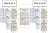 |
Fig. 1. Commander3 memory layout for map and TOD objects. The top process box represents a single computing core. |
Map objects (shown as light blue boxes in Fig. 1) are used to represent astrophysical components, spatially varying parameters, beam functions and many other things, and are distributed according to the libsharp parallelization scheme (Reinecke & Seljebotn 2013). This choice is based on the fact that libsharp is the most efficient spherical harmonics transform library available in the CMB field today, and optimizing this operation is essential. Each map object can simultaneously be expressed as pixels or a set of al, m components in harmonic space, and libsharp uses fast SHTs to convert between these two representations. Each core is given a subset of pixels and al, m coefficients, and for two maps with the same HEALPix resolution Nside, any given core will receive exactly the same pixels of each map, which helps minimize the amount of overhead for cross-frequency local operations. For maps with different Nside, there will be no correspondence between the sky areas that are assigned to each core, so each cross-resolution operation requires a full-sky broadcast operation. The header for each map (which includes information such as Nside, ℓmax, nmap6, pixel and aℓm lists for the current core, etc.) is stored as a pointer to an object called mapinfo (dark blue in Fig. 1), which itself is only stored once per unique combination of {Nside,ℓmax, nmap} to save memory.
A single TOD object (shown as yellow boxes in Fig. 1) represents all time ordered data (TOD) from one set of detectors at a common frequency or, equivalently, all the data one would want to combine into a single frequency map. These objects are generally very large, to the point where it is barely feasible to hold a single copy in memory. Therefore, the TODs are divided into discrete time chunks of a reasonable length, and distributed across cores. To minimize the memory footprint, all ancillary TOD objects (for instance, flags and pointing) are stored in memory in compressed format, as described in Sect. 4.1, and must be decompressed before any timestream operations can be performed. Thus, each chunk is processed sequentially, with the first step being decompression into standard time ordered arrays with common indexing. Those local data objects are then utilized and cleaned up before processing the next chunks. All inputs required for global TOD operations (such as gain sampling or map binning; see step 2 in Listing 1), are co-added on the fly during this iteration over chunks, and synchronization across cores is done only once after the full iteration.
Finally, to further minimize the memory footprint during the TOD binning phase (during which each core in principle needs access to pixels across the full sky), TODs are distributed according to their local sky coverage. For Planck, this implies that any single core processes pointing periods for which the satellite spin axis are reasonably well aligned, and the total sky coverage per core is typically 10% or less. This also minimizes network communication overhead during the synchronization stage.
3. The Commander3 software
In this section, we give a walk-through of the Commander3 software package, organized roughly according to the order in which a new user will experience the code. That is, we start with the code base, installation procedure, and documentation, before describing the Commander parameter file. Then we consider the actual code, and describe the main modules.
3.1. Code base, documentation, installation, and execution
The Commander code base, installation procedure, and documentation is described by Gerakakis et al. (2023), with a particular emphasis on reproducability. In short, the code is made publicly available on GitHub7 under a GNU General Public Library (GPL) license, and the documentation8 is also hosted at the same site.
At present, only Linux- and MPI-based systems are supported, and the actual installation procedure is CMake-based, and may in an ideal case be as simple as executing the following command line commands:
> git clone https://github.com/Cosmoglobe/Commander.git
> mkdir Commander/build && cd Commander/build
> cmake -DCMAKE_INSTALL_PREFIX=HOME/local \
        -DCMAKE\_C\_COMPILER=icc \
        -DCMAKE\_CXX\_COMPILER=icpc \
        -DCMAKE\_Fortran\_COMPILER=ifort \
        -DMPI\_C\_COMPILER=mpiicc \
        -DMPI\_CXX\_COMPILER=mpiicpc \
        -DMPI\_Fortran\_COMPILER=mpiifort \
        ..
> cmake --build . --target install -j 8
In this particular example, we use an Intel compiler suite, but the code has also been tested with GNU compilers. The first command downloads the source code; the second command creates a local directory for the specific compiled version; the third command creates a CMake system-specific compilation recipe (similar to Makefile) that accounts for all dependent libraries, such as HEALPix, FFTW9, and libsharp; and the fourth command actually downloads and compiles all required libraries and executables. In practice, problems typically do emerge on any new system, and we refer the interested (or potentially frustrated) reader to the full documentation for further information.
Once the code is successfully compiled, it is run through the system MPI environment, for instance
mpirun -n {ncore} path/to/commander param.txt
Specific MPI runtime environment parameters must be tuned according to the local system.
3.2. The Commander parameter file
After successfully compiling and running the code, the next step in the process encountered by most users is to understand the Commander parameter file. This is a simple human readable and editable ASCII file with one parameter per line, on the form The value cannot contain blank spaces (as anything following a space in the same line is ignored, and can be used for comments) or quotation marks, which serve a reserved internal purpose.
PARAMETER_NAME = {value}
The Commander parameter file can become very long for multi-experiment configurations, as in several thousands of lines, and maintaining readability is essential for effective debugging and testing purposes. For help in this respect, the Commander parameter file supports four special directives that allow the construction of nested parameter files, namely
  @INCLUDE {filename_with_full_path}
  @DEFAULT {filename_with_relative_path}
  @START {number}
  @END {number}
The first two of these simply insert the full contents of the specified parameter file at the calling location of the directive, and the only difference between them is whether the filename specifies a full path (as in the first case) or a path relative to a library of default parameter files (as in the second case). Nested include statements are allowed, and it is always the last occerance of a given parameter that is used. The last two directives replace any occurrence of multiple ampersands between @START and @END with the specified number.
The default parameter file library is provided as part of the Commander source code, and the path to this must be specified through an environment variable called COMMANDER_PARAMS_DEFAULT. This library contains default parameter files for each data set (Planck LFI 30 GHz, WMAP Ka-band, etc.), as well as for each supported signal component (CMB, synchrotron, thermal dust emission, etc.), and allow for simple construction of complex analysis configurations through the use of well-defined parameter files per data set and component. These also serve as useful templates when adding new experiments or components.
Parameters may also be submitted with double dashes on the command line at runtime (e.g., −−BASE_SEED=4842), to support convenient scripting. Any parameter submitted through the command line takes preference over those defined in the parameter file.
The entire parameter file is parsed and validated as the very first step of the code execution, and stored in an internal data structure called comm_params for later usage. This is done to catch user errors early in the process, and speed up debugging and testing. The internal parameter data structure is also automatically written to the output directory for reproducibility purposes.
An example of a top-level Commander parameter file with two frequency maps (Planck LFI 30 and 44 GHz) and two astrophysical components (CMB and synchrotron emission) is shown in Listing 2. A full description of all supported parameters is provided in the online documentation referenced above. We do note, however, that the quick pace of code development sometimes leaves the documentation out-of-date. If this happens, we encourage the reader to submit an issue through the GibHub repository, or simply fix it, and submit a pull request; Commander is an Open Source project, and community contributions are much appreciated.
3.3. Source code overview
After being able to run the code and edit the parameter file, the next step is usually to modify the actual code according to the needs of a specific analysis, whether it is to add support for a new astrophysical component or a new low-level TOD processing type. Clearly, this process may feel somewhat intimidating, given that the current code base currently spans more than 60 000 lines distributed over 96 different Fortran modules. Fortunately, as already mentioned, the code is highly modular in structure, and any given development project can in most cases only focus on a relatively small part of the code to achieve its goals. The goal of the current section is to provide a “code map” that helps the user to navigate the code.
This map is shown in Fig. 2 in terms of main modules. Each colored block represents one Fortran module with the name given in bold. (The gray utility box is a special case, in which each entry indicates a separate module.) Different colors represent different module types, namely data objects (green), astrophysical component objects (red), signal sampling interfaces (purple), utility routines (gray), as well as the main program (orange). We note that this map is not exhaustive, as new modules are added regularly.
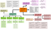 |
Fig. 2. Overview of the Commander source code. The main program is called commander.f90 and is indicated by the orange box in the center. All other boxes represents individual modules, except the gray box to the right, which summarizes various utility modules. |
The starting point for any new user is typically the main program file, commander.f90. This file implements the overall execution structure that was outlined in Listing 1, which may be divided into module initialization and main Gibbs
**************************************************
* Commander parameter file *
**************************************************
@DEFAULT LFI_tod.defaults

OPERATION = sample # { sample , optimize}

##################################################
# Algorithm specification #
##################################################

# Monte Carlo options
NUMCHAIN = 1 # Number of independent chains
NUM_GIBBS_ITER = 1500 # Length of each Markov chain
INIT_CHAIN01 = / path / to / chain / chain_init_v1.h5:1

SAMPLE_SIGNAL_AMPLITUDES = . true .
SAMPLE_SPECTRAL_INDICES = . true .
ENABLE_TOD_ANALYSIS = . true .

##################################################
# Output options #
##################################################

OUTPUT_DIRECTORY = chains_BP10

##################################################
# Data sets #
##################################################

DATA_DIRECTORY = / path / to / workdir / data
NUMBAND = 2

INCLUDE_BAND001 = . true . # 30 GHz
INCLUDE_BAND002 = . true . # 44 GHz

# 30 GHz parameters
@START 001
@DEFAULT bands / LFI / LFI_030_TOD . defaults
BAND_MAPFILE&&& = map_030_BP10 . 1 _v1 . fits
BAND_NOISEFILE&&& = rms_030_BP10 . 1 _v1 . fits
BAND_TOD_START_SCANID&&& = 3
BAND_TOD_END_SCANID&&& = 44072
@END 001

# 44 GHz parameters
@START 002
@DEFAULT bands / LFI / LFI_044_TOD . defaults
BAND_MAPFILE&&& = map_044_BP10.1_v1 . fits
BAND_NOISEFILE&&& = rms_044_BP10.1_v1 . fits
@END 002

##################################################
# Model parameters #
##################################################

NUM_SIGNAL_COMPONENTS = 2
INCLUDE_COMP01 = . true . # CMB
INCLUDE_COMP02 = . true . # Synchrotron

# CMB
@START 01
@DEFAULT component s / cmb / cmb_LFI . defaults
COMP_INPUT_AMP_MAP&& = cmb_amp_BP8 . 1 _v1 . fits
COMP_MONOPOLE_PRIOR&& = monopole?dipole : mask . fits
@END 01

# Synchrotron component
@START 02
@DEFAULT components / synch / synch_LFI . defaults
COMP_INPUT_AMP_MAP&& = synch_amp_BP8 . 1 _v1 . fits
COMP_INPUT_BETA_MAP&& = synch_beta_BP8 . 1 _v1 . fits
COMP_PRIOR_GAUSS_BETA_MEAN&& = ?3.3
@END 02
Listing 2. Prototype Commander parameter file.
operations, and spans only about 500 lines of code. From this module, one may follow the arrows in Fig. 2 to identify any specific submodule.
3.3.1. Data infrastructure
The main data interface is defined in comm_data_mod, in terms of a class called comm_data_set. Each object of this type represents one frequency channel, for instance Planck 30 GHz, WMAP Q-band, or Haslam 408 MHz. The main class definition is shown in Listing 3, which is common to all data objects. The top section defines various scalars, such as the frequency channel label (e.g., LFI_030), unit type (e.g., μK), number of detectors, and TOD type (if any). The next section defines pointers to various map-level objects, including the actual co-added frequency map, main and processing masks, and the data-minus-model residual. All of these share the same mapinfo instance, as outlined in Fig. 1, stored in info.
The noise model is defined in terms of a pointer to an abstract and generic comm_N class (implemented in comm_N_mod in Fig. 2), which is instantiated in terms of a specific subclass. At the moment, only three noise types are supported, namely spatially uncorrelated white noise (Npp′ = σpδpp′, implemented in comm_n_rms_mod); a full dense low-resolution noise covariance matrix for Stokes Q and U, as defined by the WMAP data format, implemented in comm_n_qucov_mat; and white noise per pixel, but projecting out all large-scale harmonic modes with ℓ ≤ ℓcut, implemented in comm_n_lcut_mat. Each of these modules defines routines for multiplying a given sky map with operators like N−1, N−1/2, and N1/2, but does not permit access to specific individual elements (except for diagonal elements, which are used for CG preconditioning). As such, very general noise modules may easily be defined, and external routines do not have to care about the internal structure of the noise model.
Next, each data object is associated with a beam operator, B, implemented in comm_B_mod. Once again, this is an abstract class, and must be instantiated in terms of a subclass. In the current implementation, only azimuthally symmetric beams defined by a Legendre transform bℓ are supported (in comm_B_bl_mod), but future work may for instance aim to implement support for asymmetric FeBeCOP beams (Mitra et al. 2011) or time-domain total convolution (Wandelt & Górski 2001; Galloway et al. 2023).
Bandpass integration routines are implemented through the comm_bp module, and are accessible for each data set through the bp pointer. This module defines the effective bandpass, τ, per detector (if relevant) and for the full co-added frequency channel. It provides both unit conversion factors and astrophysical SED integration operations, adopting the notation of Planck Collaboration IX (2014), Svalheim et al. (2023b). The specific integration prescription must be specified according to experiment; the differences between the various cases account for instance for whether τ is defined in brightness or flux density units, or whether any thresholds are applied to τ. In general, we chose to reimplement the conventions adopted by each experiment individually, rather than modifying the inputs to fit a standard convention, to stay as close as possible to the original analyses.
Astrophysical SED bandpass integration is performed in the mixing module class, comm_F_mod10. A central step in the Commander analysis is fitting spectral parameter for each astrophysical component, and this requires repeated integration of parametric SEDs with respect to each bandpass. To avoid performing the full integral for every single parameter change, we precompute look-up tables for each component and bandpass over a grid in each parameter. For SEDs with one or two parameters, we use (bi-)cubic splines to interpolate within the grid. Separate modules are provided for constant, one- and two-dimensional SEDs, as well as δ-function SEDs (supporting line emission components). While this approach is computationally very efficient, it also introduces an important limitation, in that only two- or lower-dimensional parametric SEDs are currently supported; future work should aim to implement arbitrary dimensional SED interpolation, for instance using machine learning techniques (e.g., Fendt & Wandelt 2007).
For relevant channels, time-ordered data are stored in the abstract comm_tod class, which is illustrated in Listing 4. This structure has three levels. At the highest level, comm_tod describes the full TOD for all detectors and all scans. This object defines all parameters that are common to all detectors and scans, for instance frequency label, sampling rate, and TOD type. It also contains an array of comm_scan objects, each of which contains the TOD of a single scan for all detectors. This module defines all parameters that are common to that particular scan, for instance the number of samples in the current scan, ntod, or the satellite velocity with respect to the Sun, vSun. It also contains an array of comm_detscan objects, in which the actual data for a single scan and single detector are stored. The various data, flag and pointing arrays (tod, flag, pix, psi) are stored in terms of byte objects, which indicates that these are all Huffman compressed, as discussed in Sect. 2.4. (This feature is optional, and it is possible to store the data uncompressed). The comm_tod object provides the necessary decompression routines.
The most important TOD routine is process_tod in the comm_tod object. The main task of this routine is to produce a sky map and its noise description given an astrophysical reference sky. This includes both performing all relevant TOD-level sampling steps, and solving for the actual map either through binning or CG solvers. Since each experiment in general requires different sampling steps and mapmaking approaches,
   type comm_data_set
     character(len=512)           :: label
     character(len=512)           :: unit
     integer                      :: ndet
     character(len=128)           :: tod_type
     logical                      :: pol_only

     class(comm_mapinfo),pointer :: info
     class(comm_map),    pointer :: map
     class(comm_map),    pointer :: res
     class(comm_map),    pointer :: mask
     class(comm_map),    pointer :: procmask
     class(comm_tod),    pointer :: tod
     class(comm_N),      pointer :: N
     class(B_ptr),       allocatable, dimension(:) :: B
     class(comm_bp_ptr), allocatable, dimension(:) :: bp
   contains
     procedure :: RJ2data
     procedure :: chisq => get_chisq
  end type comm_data_set
Listing 3. Prototype Commander data class, comm_data_set.
we chose to implement one TOD module per experiment, for instance comm_tod_lfi_mod, as opposed to one super-module for all experiments with excessive use of conditional if-tests. This both makes the overall TOD processing code more readable, and it allows different people to work simultaneously on different experiments with fewer code synchronization problems11. The main costs are significant code replication and a
! TOD class for all scans, all detectors
type, abstract :: comm_tod
   character(len=512) :: freq
   character(len=128) :: tod_type
   integer            :: nmaps
   integer            :: ndet
   integer            :: nscan
   real               :: samprate
   type(comm_scan), dimension(:) :: scans
 contains
   procedure  :: read_tod
   procedure  :: process_tod
   procedure  :: decompress_tod
   procedure  :: tod_constructor
end type comm_tod

! ####################################################

! TOD class for single scan, all detectors
type :: comm_scan
   integer    :: ntod
   real       :: v_sun(3)
   class(comm_detscan), dimension(:) :: d
end type comm_scan

! ####################################################

! TOD class for single detector and single scan
type :: comm_detscan
   logical    :: accept
   class(comm_noise_psd), pointer   :: N_psd
   byte,               dimension(:) :: tod
   byte,               dimension(:) :: flag
   type(byte_pointer), dimension(:) :: pix
   type(byte_pointer), dimension(:) :: psi
Listing 4. TOD object structure used in Commander. These module descriptions are incomplete and are only intended to illustrate the structure, not the full contents.
higher risk of code divergence during development. Common operations are, however, put into general TOD modules, such as comm_tod_gain_mod and comm_tod_orbdipole_mod, with the goal of maximizing code reusability.
3.3.2. Signal model infrastructure
The red boxes in Fig. 2 summarize modules that defines the astrophysical sky model, and the purple boxes contain corresponding sampling algorithms. Starting with the former, we see that three fundamentally different types of components are currently supported, namely (1) diffuse components, (2) point source components, and (3) template components. The first of these is by far the most important, as it is used to describe the usual spatially varying “full-sky” components, such as CMB, synchrotron and thermal dust emission. The main difference between the various diffuse components are their spectral energy densities (SEDs) that defines the signal strength as a function of frequency in units of brightness temperature, with some set of free parameters. Examples of currently supported SEDs are listed in the bottom right block of Fig. 2. We note, however, that it is very easy to add support for a new SED type as follows. First, we determine how many free spectral parameters the new component should have; if it is less than or equal to two, then we identify an existing component with the same number of parameters, and copy and rename the corresponding module file. Then we edit the function called evalSED in that routine to return the desired parametric SED. Finally, we search for all occurrences of the original component label in the comm_signal_mod module, and add corresponding entries for the new component. Typically, adding a new SED type with two or fewer parameters can be done in 15 min; if the component has more than two free parameters, however, new mixing matrix interpolation and precomputation infrastructure has to be implemented, as discussed above.
The spatial distribution of a diffuse component is defined in terms of a spherical harmonics expansion,  , with an upper frequency cutoff, ℓmax, coupled to the SED discussed above. Optionally, the spherical harmonics coefficients may be constrained through an angular power spectrum, Cℓ ≡ ⟨|aℓm|2⟩, that intuitively quantifies the smoothness of the component through the signal covariance matrix, S (Andersen et al. 2023). Currently supported power spectrum modes include
binned: Dℓ ≡ Cℓℓ(ℓ+1)/2π is piecewise constant within user-specified bins; typically the default choice for the CMB component (Colombo et al. 2023; Paradiso et al. 2023);
power_law: Dℓ = q(ℓ/ℓ0)α, where q is an amplitude, ℓ0 is a pivot multipole, and α is a spectral slope; often used for astrophysical foregrounds, such as synchrotron or thermal dust emission (e.g., Planck Collaboration X 2016);
gauss: Dℓ = q exp(−ℓ(ℓ+1)σ2), where σ is a user-specified standard deviation; used to impose a natural smoothing scale to suppress Fourier ringing;
none: no power spectrum prior is applied, S−1 = 0.
Support for integrated cosmological parameter models through CAMB (Lewis et al. 2000) is on-going. When complete, this will be added as a new type for which S will be defined in terms of the usual cosmological parameters (H0, Ωi, τ, etc.).
Point source components are defined through a user-specified catalog of potential source locations, following Planck Collaboration IV (2020). Each source is intrinsically assumed to be a spatial δ function, with an amplitude defined in units of flux density in milli-Janskys. Each source location is then convolved with the local instrumental beam shape of each channel (typically asymmetric FeBeCOP beam profiles for Planck, Mitra et al. 2011, and azimuthally symmetric beam profiles for other experiments), and this is adopted as a spatial source template at the relevant frequency channel. In addition, each source is associated with an SED, similar to the diffuse components, allowing for extrapolation between frequencies. Currently supported models include power-law (for radio sources), modified blackbody (for far-infrared sources), and thermal Sunyaev-Zeldovich SEDs. Time variability is not yet supported.
Finally, template components are defined in terms of a user-specified fixed template map for which the only free parameter is an overall amplitude at each frequency. This is primarily included for historical reasons, for instance to support template fitting as implemented by the WMAP team (Bennett et al. 2013). However, this approach allows very limited uncertainty propagation, and we therefore generally rather prefer to include relevant survey maps (for instance the 408 MHz survey by Haslam et al. 1982) as additional frequency channels, for which meaningful uncertainties per pixel may be defined. This mode is not used in the current BEYONDPLANCK analysis (BeyondPlanck Collaboration 2023).
The purple boxes in Fig. 2 contain sampling routines for these parameters, and these are split into two categories; linear and nonlinear. The linear parameters (i.e., component amplitude parameters) are sampled using a preconditioned CG solver (Seljebotn et al. 2019), as implemented in the comm_cr_mod (“Constrained Realization”) module, while the nonlinear spectral parameters are sampled in the comm_nonlin_mod module using a combination of Metropolis and inversion samplers (Andersen et al. 2023; Svalheim et al. 2023a).
4. Optimization
The Commander walk-through given in Sect. 3 is high-level in nature, and is intended to give a broad overview of the code. In this section, we turn our attention to lower-level details, and focus in particular on specific optimization challenges and tricks that improve computational efficiency.
4.1. In-memory data compression
As discussed in Sect. 2.4, one of the key challenges for achieving efficient end-to-end CMB analysis is memory management; since the full TOD are required at every single Gibbs iteration, it is imperative to optimize data access rates. In that respect, we first note that RAM read rates are typically at least one order of magnitude higher than disk read rates, and, second, most TOD operations are bandwidth limited simply because each sample is only used once (or a few times) per read. For this reason, a very useful optimization step is simply to be able to store the full TOD in RAM. At the same time, we note that disk space is cheap, while RAM is expensive. It is therefore also important to minimize the total data volume.
We address this issue by storing the TOD in a compressed form in RAM, and decompress each data segment before further processing at run-time. In the current implementation, we adopt Huffman coding (Huffman 1952), and implement the decompression algorithms natively in the source code; of course, other lossless compression algorithms can be used, and in the future it may be worth exploring using different algorithms for different types of objects.
Typically, most current CMB experiments distribute their data, as recorded by analog-to-digital converters (ADCs), in the form of 32-bit integers, which support over 2 billion different numbers; we will refer to each distinct integer as a “symbol” in the following. However, the actual dynamic range of any given data segment only typically spans a few thousand different symbols. Therefore, simply by choosing a more economic integer precision level, a factor of three could be gained. Further improvements could be made by actually counting the frequency of each symbol separately, and assign short bit strings to frequently occuring symbols, and longer bit strings to infrequently occuring symbols. Huffman coding is a practical algorithm that achieves precisely this, and it can be shown to be the theoretically optimal lossless compression algorithm when considering each datum separately. To account for correlations, noting that most CMB TODs are correlated in time, we difference all datastreams sample-by-sample prior to compression, setting  ; after this differencing, most data values will be close to zero.
The actual Huffman encoding relies on a binary tree structure, and assigns numbers with high frequencies to short codes near the top of the tree, and infrequent numbers to long codes near the bottom. As a practical and real-life example, Fig. 3 shows the top of the Huffman encoding tree for the arbitrarily selected PID 27 646 for the 30 GHz data. In this case, 0 represents about 42% of the entire data set after the pair-wise differencing operation. The optimal compression is therefore to represent 0 with a single bit (which also happens to be 0), and numbers that occur frequently, such as 1 and −1, with 4-bit codes (1110 and 1001, respectively). At the bottom of the tree are those numbers which occur very infrequently. This diagram is obviously truncated, and the full tree uses codes with lengths of 20 bits to represent the lowest symbols that occur only once. A simple worked example of Huffman coding is given in Appendix A.
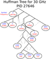 |
Fig. 3. Truncated Huffman tree for the compression of the LFI 30 GHz channel at Nside = 512 on PID 27 646. The ovals represent the “leafs” of the tree, each of which contains a single number to be compressed. To determine the symbol that represents each number in the Huffman binary array, simply read down the tree from the top, adding a 0 for every left branch and a 1 for every right branch. The number −2, for example, is in this table represented by the binary code 11010. Dotted lines represent branches that were truncated for visual reasons. The full tree contains 670 unique numbers with a total array size of 861 276 entries. |
The Huffman algorithm requires a finite number of symbols to be encoded, and therefore performs far better for integers than for floats. This is intrinsically the case for (ADC-outputted) TOD and flag information, but not for pointing values. However, as most modern CMB experiments, BEYONDPLANCK uses HEALPix to discretize the sky. Precomputing the HEALPix coordinates of each sample therefore allows the pointing sky coordinates to be reduced from two floats per sample (representing θ and ϕ) to one single integer. Of course, this requires the HEALPix resolution parameter, Nside, to be predefined during data preprocessing and compression for each band. In practice, this is acceptable as long as Nside is selected to correspond to a higher resolution than the natural beam smoothing scale of the detectors. For the LFI 30 and 44 GHz channels, we adopt Nside = 512, whereas for the 70 GHz channel we adopt Nside = 102412. We note that this is indeed a lossy compression step, but it is precisely the same lossy compression that is always involved in CMB mapmaking; the only difference is that the discretized pointing is evaluated once as a preprocessing step.
The same does not hold for the polarization angle, ψ, which also is a float, and typically is not discretized in most current CMB mapmaking codes. However, as shown by Keihänen & Reinecke (2012) in the context of beam deconvolution for LFI through the use of so-called 4D maps, even this quantity may be discretized with negligible errors as long as a sufficient number of bins between 0 and 2π is used. Specifically, Keihänen & Reinecke (2012) used nψ = 256 bins for all LFI channels, while for BEYONDPLANCK we adopt nψ = 4096; the additional resolution has an entirely negligible cost in terms of increased Huffman tree size.
To check the impact of the polarization angle compression, Fig. 4 shows difference Stokes T, Q, and U maps for the co-added 30 GHz frequency channel generated in two otherwise identical mapmaking runs with nψ = 4096 and 32 768. Here we see that the compression introduces artifacts at the level of 0.01 μK at high Galactic latitudes, increasing to about 0.1 μK in the Galactic plane, which is entirely negligible compared to the intrinsic uncertainties in these data, fully confirming the conclusions of Keihänen & Reinecke (2012).
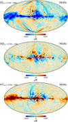 |
Fig. 4. 30 GHz T, Q, and U map differences between two pipeline executions using different levels of compression (nψ = 32 768 and nψ = 4096), smoothed by a 1° beam. The differences in temperature look like correlated noise, and in polarization we have some leakage from polarized synchrotron. In both cases, the amplitude of the differences is much lower than the uncertainties from other effects. |
The main cost associated with Huffman compression comes in the form of an additional cost for decompression prior to TOD processing. Specifically, we find that decompression costs about 10% of the total runtime per iteration; we consider this to be an acceptable compromise to enable the entire data set to be held in memory at once and eliminate disk read time.
Table 1 gives an overview of the compression performance for each data object and LFI frequency channel. Overall, we see that the TOD data volume is reduced by a factor of about six, while the pointing volume is reduced by a factor of about 20.
Huffman compression performance for each Planck LFI data object and frequency channel.
4.2. FFT optimization and aliasing mitigation
Once the data are stored in memory, the dominant TOD operation are the FFTs, which are used repeatedly for both correlated noise and gain sampling (Ihle et al. 2023; Gjerløw et al. 2023). Fortunately, several highly optimized FFT libraries are widely available that provides outstanding performance, and we currently adopt the FFTW implementation (Frigo & Johnson 2005).
Still, there are several issues that needs to be considered regarding FFTs. The first regards runtime versus the length of each data segment. In particular, the FFTW documentation notes that
“FFTW works most efficiently for arrays whose size can be factored into small primes (2, 3, 5, and 7).”
As an illustration of this fact, Fig. 5 shows the time per FFT as a function of data length, as measured on a local compute cluster; the top panel shows all lengths up to 10 000, while the bottom panel shows a zoom-in of the top panel. Here we clearly see that run times can vary by at least an order of magnitude from one length to the next.
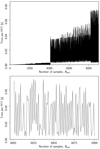 |
Fig. 5. FFT costs computed as a function of window length. Top: cost per FFT as a function of FFT length. Bottom: zoom-in of the top panel, showing more details of the variation within a small sample range. |
Commander3 exploits this effect at read-in time. As each chunk of data is read, its length is compared to a precomputed table of FFT costs for all values up to Nsamp = 106. The data chunk is then truncated to the nearest local minima of the cost function, losing only a small amount of data (0.03%) while providing a large speedup for all FFT operations performed on that chunk. Of course, if the noise stationarity length is unconstrained, and the segment length is fully up to the user to decide, then powers of 2n are particularly desirable.
Another important effect to take into account is that of FFT aliasing and edge effects; the underlying FFT algebra assumes by construction that the data in question are perfectly periodic. If there are notable gradients extending through the segment, the end of the segment may have a significantly different mean than the beginning, and this will be interpreted by the FFT as a large discrete jump. If any filtering or convolution operators (for instance inverse noise weighting, N−1) are applied to the data, this step will result in nonlocalized ringing that can contaminate the data.
Several approaches to mitigate this effect are described in the literature, and zero padding is perhaps one of the best known, in which one adds zeros to both ends of the original data stream. However, this operation also has a nontrivial impact on the outcome, and we chose a more expensive and more conservative approach, namely mirroring: Before every FFT operation, we double the length of the array in question, and add a mirrored version of the original array into the second half. This makes the function periodic by construction, and eliminates any discrete boundary effects. However, this safety does come at a price of doubling the run time, and future implementations should explore alternative approaches. One possibility is to allow for data duplication in overlap regions, such that for instance 5% of a given data segment is filled by data from the neighboring segments at both edges. Then the overlap region is discarded after filtering. This approach was explored by Galloway (2019), and shown to work very well for SPIDER noise modeling.
4.3. Conjugate gradient optimization for component separation
The second most important numerical operation in the BEYONDPLANCK Gibbs sampler after FFTs is the spherical harmonics transform. This forms the numerical basis for the astrophysical component amplitude sampler (Andersen et al. 2023), in which the following equation is solved repeatedly (Seljebotn et al. 2019),
Here S and Nν denote the signal and noise covariance matrices, respectively, Mν is a mixing matrix, mν is an observed frequency map, a is a vector containing all component amplitudes, and Y is a spherical harmonics transform. In this expression, Nν, Mν, and mν are all defined as pixelized map vectors, while S and a are defined in spherical harmonic space, and Y converts between the two spaces.
Equation (10) involves millions of free parameters, and must therefore be solved iteratively with preconditioned CG-type methods (Shewchuk 1994). There are therefore two main approaches to speed up its solution: Either one may reduce the computational cost per CG iteration, or one may reduce the number of iterations required for convergence. As far as the former approach is concerned, by far the most important point is simply to use the most efficient SHT library available at any given time to perform the Y operation; all other operations are linear in the number of pixels or spherical harmonics coefficients, and are largely irrelevant as far as computational costs are concerned. At the time of writing, the fastest publicly avaialble SHT library is libsharp2 (Reinecke & Seljebotn 2013), and we employ its MPI version for the current calculations. (We note that the OpenMP version is even faster, but since the current Commander3 parallelization strategy is agnostic with respect to compute nodes, and all data are parallelized across all available nodes, this mode is not yet supported).
The main issue to optimize is therefore the number of iterations required for convergence. Again, there are two different aspects to consider, namely preconditioning and the stopping criterion. Starting with the former, we recall that a preconditioner is simply some (positive definite) linear operator, P, that is applied to both sides of Eq. (10) in the hope that the equation becomes easier to solve numerically. The ideal case is that P is equal to the inverse of the coefficient matrix on the left-hand side, but this is of course never readily available; if it were, the system would already be solved. In the current work, we adopt the preconditioner introduced by Seljebotn et al. (2019) for Eq. (10), which approximates the inverse of a non-square matrix, A, by its pseudo-inverse A+ ≡ (AtA)−1At. A possible future improvement might be to replace this on large angular scales with the exact brute-force block preconditioner of Eriksen et al. (2004b, 2008) for ℓ ≲ 100.
The final question is then, simply, to determine how many CG iterations are required to achieve acceptable accuracy. To address this issue, we solve Eq. (10) for the basic BEYONDPLANCK configuration (BeyondPlanck Collaboration 2023) with a maximum of 1000 iterations, and plot the rms difference between the CMB solutions obtained at the ith and 1000th iterations. This quantity is plotted in Fig. 6. Here we see that that the residual decreases rapidly up to about 70 iterations, while for more than 100 iterations only very modest differences are seen. For the final BEYONDPLANCK runs, we have chose 100 iterations as the final cutoff.
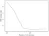 |
Fig. 6. rms of a CMB difference map comparing various iteration numbers to the most converged 1000 iteration case. The rms drops rapidly until about 50 samples, at which point the marginal increase in convergence per sample flattens out. |
We note that this criterion differs from most previous Commander-based analyses (e.g., Planck Collaboration X 2016), which usually have defined the cutoff in terms of a relative reduction of the preconditioned residual, r = ||Ax − b)|2. The reason we prefer to define the convergence criterion in terms of map-level residuals with respect to the converged solution is simply that r may weight the various astrophysical components very differently, for instance according to arbitrarily chosen units. One example is synchrotron emission, which has a reference frequency of 408 MHz in the BEYONDPLANCK analysis, and is measured in units of μKRJ, and therefore has a much higher impact on r than the CMB component. If we were to use the preconditioned residual as a threshold instead (which many analyses also do), then nearly singular modes in A may be given a relatively large weight. In practice, it is our experience that a map-based rms cutoff is less prone to spurious and premature termination than either of the two residual-based criteria.
4.4. File format comparison: HDF versus FITS
The current Commander3 implementation adopts the hierarchical data format (HDF) for TOD disk storage. While the CMB community has largely converged on the standard FITS format for maps, this format has some drawbacks that make them less than ideal for time-domain data sets, both in terms of efficiency and programming convenience. For instance, HDF files support internal directory tree structures, which allows for intuitive storage of multiple layers of information within each file. Additionally, HDF can easily support data sets with different lengths, which is useful when handling compressed data. Finally, the HDF format supports headers and metadata for every data set, which makes it very easy to store quantities such as units, conversion factors, compression information and even human-readable help strings locally.
Most importantly, however, is simply the fact that HDF is faster than FITS. To quantify this, we performed several timing tests, and one example is shown in Fig. 7. In this case, we write a given data subset of varying size (single-detector 27M, single-horn 27M+S and the full 30 GHz channel) to disk repeatedly using standard Python libraries, and we plot the ratio of the time averages required for this task. HDF operations are performed with h5py and FITS operations with astropy.io.fits. For this particular case, we see that HDF output is typically one order of magnitude faster than FITS output on our system.
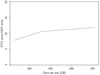 |
Fig. 7. Ratio between FITS and HDF disk write times for subsets of the LFI data of various sizes. |
5. Resource requirements
At the outset of the BEYONDPLANCK project, it was by no means obvious whether full end-to-end Bayesian processing was computationally feasible with currently available computing resources. A main goal of the general project in general, and this paper in particular, was therefore simply to quantify the resource requirements for end-to-end Bayesian CMB analysis in a real-life setting, both in terms of CPU hours and RAM. These are summarized for the main BEYONDPLANCK run, as defined in BeyondPlanck Collaboration (2023), in Table 2. All processing times refer to total CPU hours integrated over computing cores, and since each chain is parallelized over 128 cores, all numbers may be divided by that number to obtain wall hours.
Computational resources required for end-to-end BEYONDPLANCK processing.
Starting with the data volume, we see that the total raw LFI TOD span almost 8 TB as provided by the Planck Data Processing Center (DPC). After compression and removing non-essential information, this is reduced by almost an order of magnitude, as the final RAM requirements for LFI TOD storage is only 861 GB. The total RAM requirement for the full job including component separation (most of which is spent on storing the full set of mixing matrices per astrophysical component and detector) is 1.5 TB.
The second section shows the total initialization time, which accounts for the one-time cost of reading all data into memory. This is mostly dominated by disk read times, so systems with faster disks will see improvements here. However, as this is only executed at the start of the run, it is a very subdominant cost compared to the loop execution time.
The bottom section of Table 2 summarizes the computational costs for a single iteration of the Gibbs sampling loop. Here we see that the total cost per sample is dominated by the TOD sampling loop (as would be naively expected from data volume), which takes about 59% of the full sample time. The remaining 41% is spent on component separation; about one third of this is spent on amplitude sampling (as discussed in Sect. 4.3), and two-thirds is spent on spectral parameter sampling. The former of these is fairly well optimized, as it is dominated by SHTs, while the latter clearly could be better optimized, for a potential maximum saving of 25% of the total runtime.
For the 70 GHz channel, 35% of the total processing time is spent on correlated noise sampling, P(ncorr|d, …). This step is by itself the most computationally complex and expensive operation, as it requires FFTs within a CG solver for correlated noise gap filling (Ihle et al. 2023). This step could be sped up through approximations, but we found that the CG solver was the only way to guarantee high accuracy in regions with large processing masks, most notably scans through the Galactic plane. For the 30 and 44 GHz channels, the most expensive operation is in fact correlated noise PSD sampling, P(ξcorr|d, …), and this is an indication of sub-optimality of the current implementation, rather than a fundamental algorithmic bottleneck: One of the last modifications made to the final BEYONDPLANCK pipeline was the inclusion of a Gaussian peak in the noise PSD around 1 Hz, and this operation was not optimized before the final production run. Future implementations should be able to reduce this time to negligible levels, as only low-volume power spectrum data are involved in noise PSD sampling.
Next, we see that the Huffman decompression costs about 10% of the total runtime, and we consider this to be a fair price to pay for significantly reduced memory requirements. Indeed, without Huffman compression we would require multi-node MPI communication, and in that case many other operations would become significantly more expensive. Thus, it is very likely that Huffman coding in fact leads to both lower memory requirements and reduced total runtime.
We also see that sidelobe evaluation accounts for about 10% of the total runtime, most of which is spent on interpolation. This part can also very likely be significantly optimized, and the ducc13 library appears to be a particularly promising candidate for future integration. Sidelobe evaluation will become even more important for a future WMAP analysis, for which four distinct detector TODs are combined into a single differencing assembly TOD prior to noise estimation and mapmaking, each with its own bandpass (Bennett et al. 2013). Actually, as reported by Watts et al. (2023), sidelobe interpolation currently accounts for about 20% of the total WMAP runtime due to this structure.
Unaccounted for TOD processing steps represent a total of 12% of the total low-level processing time and include both actual computations, such as χ2 evaluations and bandpass sampling, and loss due to poor load balancing. The latter could clearly be reduced in future versions of the code.
Overall, we see from Table 2 that up to 74 h per sample (sidelobe evaluation, correlated noise PSD sampling, spectral index sampling, and other TOD costs) can potentially be gained through more careful optimization within the current coding paradigm, or about half of the total runtime. This optimization will of course happen naturally in the future, as each module gradually matures. Also, the current native Commander3 code does not yet support vectorization (SSE, AVX, etc.) natively, but only partially through the external FFT and SHT libraries, and whatever the Fortran compiler can manage on its own. This will also be done in future work.
Finally, it is important to note that the current analysis framework is inherently a Markov chain, and that means that each sample depends directly on the previous one. The Bayesian analysis approach is therefore intrinsically more challenging to parallelize than the forward simulation frequentist-style approach, for which independent realizations may be run on separate compute cores (e.g., Planck Collaboration XII 2016). As each variable in the Gibbs chain is required to hold the full previous state of the chain constant, it is difficult to find segments of the code that can run independently for long times without synchronizing. One place this could be added is in the TOD sampling step. Each of the different bands could be run independently at the same time (i.e., the 30 GHz map is independent of the 44 and 70 GHz parameters). With many TOD bands, like the configuration proposed for LiteBIRD, this could be a feasible parallelization scheme, but for LFI with only three bands the runtime is dominated by the 70 GHz processing time regardless, and this technique could shave at most 20% off the total runtime for the current run. For future analyses of massive data sets with thousands of detectors, however, data partitioning will become essential to achieve acceptable parallelization speed-up.
6. Summary and outlook
The main goal of this paper is to provide an overview of the BEYONDPLANCK infrastructure used to analyze the Planck LFI data within an end-to-end Bayesian framework, hopefully aiding new users to modify and extend it to their needs. We have discussed the various computational and architectural decisions that have been adopted for the BEYONDPLANCK codebase, as well as some of the current challenges facing the development effort. We highlight in particular the choices made for the analysis of the LFI data, but many of these architectural decisions were selected to be generalizable to future data sets.
One important novel feature introduced here that is likely to be useful for many future CMB experiments is in-memory data compression. We find that the original data volume may be reduced by one order of magnitude through data selection and compression, with negligible loss of precision. For LFI, this allows the entire data set to be stored in memory on modest computing hardware, and it reduces the disk read time to a one-time initialization cost, independent of the number of iterations of the algorithm. In general, in-memory compression permits the analysis to be performed on small clusters that are often available at individual research institutions, as opposed to national high-performance computing centers, and this has significant advantages in both cost and ease of use, for instance shorter debugging cycles and queuing times. We suggest that future experiments such as CMB S4 and Simons Observatory that are planning for data volumes many times larger than Planck’s consider using these lossless techniques to reduce the resource requirements of their overall analysis task.
We also quantify the computational costs for the BEYONDPLANCK LFI analysis, and the resulting numbers may serve as an estimate of the pipeline’s performance for future similarly sized data sets. Specifically, we find that the LFI analysis requires 1.5 TB of RAM, and producing one single sample costs about 170 CPU-hrs. This latter number may be compared with the costs required to produce the official Planck Full Focal Plane simulations. For instance, as discussed by Planck Collaboration XII (2016), producing 81 000 LFI noise simulations on the Finnish Sisu cluster cost 4 million CPU hours, for an average cost of 50 CPU-hrs/map. The current BEYONDPLANCK approach, which includes all steps from low-level calibration to final component separation and allows for the full exploration of parameter degeneracies, is therefore computationally equivalent to producing only three correlated-plus-white noise realizations in a traditional frequentist approach, which allows much more restricted error propagation. We conclude that the Bayesian approach compares favorably with respect to the traditional approach in terms of computational costs.
More generally, we conclude that the analysis pipeline described in this paper is ideally suited for moderately sized CMB data sets, and we believe that it can be extended to many existing and future experiments with relatively minor efforts. One concrete and specific example is the on-going WMAP analysis presented by Watts et al. (2023), which appears quite encouraging both in terms of computational efficiency and data quality.
While the BEYONDPLANCK project itself was a time-limited effort from 2018 to 2021, this work will be continued within the context of the Open Science and community-wide COSMOGLOBE project. We strongly encourage all interested parties to get involved in that project, and together develop an Open Source state-of-the-art model of CMB sky.
Acknowledgments
We thank Prof. Pedro Ferreira and Dr. Charles Lawrence for useful suggestions, comments and discussions. We also thank the entire Planck and WMAP teams for invaluable support and discussions, and for their dedicated efforts through several decades without which this work would not be possible. The current work has received funding from the European Union’s Horizon 2020 research and innovation programme under grant agreement numbers 776282 (COMPET-4; BEYONDPLANCK), 772253 (ERC; BITS2COSMOLOGY), and 819478 (ERC; COSMOGLOBE). In addition, the collaboration acknowledges support from ESA; ASI and INAF (Italy); NASA and DoE (USA); Tekes, Academy of Finland (grant no. 295113), CSC, and Magnus Ehrnrooth foundation (Finland); RCN (Norway; grant nos. 263011, 274990); and PRACE (EU).
References
- Ade, P., Aguirre, J., Ahmed, Z., et al. 2019, JCAP, 2019, 056 [Google Scholar]
- Andersen, K. J., Herman, D., Aurlien, R., et al. 2023, A&A, 675, A13 (BeyondPlanck SI) [NASA ADS] [CrossRef] [EDP Sciences] [Google Scholar]
- Basyrov, A., Suur-Uski, A.-S., Colombo, L. P. L., et al. 2023, A&A, 675, A10 (BeyondPlanck SI) [NASA ADS] [CrossRef] [EDP Sciences] [Google Scholar]
- Bennett, C. L., Banday, A. J., Gorski, K. M., et al. 1996, ApJ, 464, L1 [NASA ADS] [CrossRef] [Google Scholar]
- Bennett, C. L., Hill, R. S., Hinshaw, G., et al. 2003, ApJS, 148, 97 [Google Scholar]
- Bennett, C. L., Larson, D., Weiland, J. L., et al. 2013, ApJS, 208, 20 [Google Scholar]
- BeyondPlanck Collaboration (Andersen, K. J., et al.) 2023, A&A, 675, A1 (BeyondPlanck SI) [Google Scholar]
- Bobin, J., Starck, J., Fadili, J., & Moudden, Y. 2007, IEEE Trans. Image Process., 16, 2662 [NASA ADS] [CrossRef] [Google Scholar]
- Cardoso, J.-F., Le Jeune, M., Delabrouille, J., Betoule, M., & Patanchon, G. 2008, IEEE J. Sel. Top. Signal Process., 2, 735 [CrossRef] [Google Scholar]
- Carlstrom, J., Abazajian, K., Addison, G., et al. 2019, Bull. Am. Astron. Soc., 51, 209 [Google Scholar]
- Cheng, E. 1992, Astron. Data Anal. Softw. Syst., 25, 368 [NASA ADS] [Google Scholar]
- Colombo, L. P. L., Eskilt, J. R., Paradiso, S., et al. 2023, A&A, 675, A11 (BeyondPlanck SI) [NASA ADS] [CrossRef] [EDP Sciences] [Google Scholar]
- Delabrouille, J., Cardoso, J. F., Le Jeune, M., et al. 2009, A&A, 493, 835 [NASA ADS] [CrossRef] [EDP Sciences] [Google Scholar]
- Eriksen, H. K., Banday, A. J., Górski, K. M., & Lilje, P. B. 2004a, ApJ, 612, 633 [Google Scholar]
- Eriksen, H. K., O’Dwyer, I. J., Jewell, J. B., et al. 2004b, ApJS, 155, 227 [Google Scholar]
- Eriksen, H. K., Jewell, J. B., Dickinson, C., et al. 2008, ApJ, 676, 10 [Google Scholar]
- Fendt, W. A., & Wandelt, B. D. 2007, ArXiv e-prints [arXiv:0712.0194] [Google Scholar]
- Fernández-Cobos, R., Vielva, P., Barreiro, R. B., & Martínez-González, E. 2012, MNRAS, 420, 2162 [Google Scholar]
- Frigo, M., & Johnson, S. G. 2005, Proc. IEEE, 93, 216 [Google Scholar]
- Galloway, M. 2019, PhD thesis, University of Toronto, Canada [Google Scholar]
- Galloway, M., Reinecke, M., Andersen, K. J., et al. 2023, A&A, 675, A8 (BeyondPlanck SI) [NASA ADS] [CrossRef] [EDP Sciences] [Google Scholar]
- Gerakakis, S., Brilenkov, M., Ieronymaki, M., et al. 2023, Open J. Astrophys., 6, 10 [NASA ADS] [Google Scholar]
- Gjerløw, E., Ihle, H. T., Galeotta, S., et al. 2023, A&A, 675, A7 (BeyondPlanck SI) [NASA ADS] [CrossRef] [EDP Sciences] [Google Scholar]
- Gorski, K. M., Hivon, E., Banday, A. J., et al. 2005, ApJ, 622, 759 [Google Scholar]
- Gutiérrez, C. M., Davies, R. D., Watson, R. A., et al. 1996, Astron. Astrophys. Trans., 10, 43 [CrossRef] [Google Scholar]
- Haslam, C. G. T., Salter, C. J., Stoffel, H., & Wilson, W. E. 1982, A&AS, 47, 1 [NASA ADS] [Google Scholar]
- Hazumi, M., Ade, P., Akiba, Y., et al. 2019, J. Low Temp. Phys., 194, 443 [NASA ADS] [CrossRef] [Google Scholar]
- Hinshaw, G., Barnes, C., Bennett, C. L., et al. 2003, ApJS, 148, 63 [NASA ADS] [CrossRef] [Google Scholar]
- Huffman, D. A. 1952, Proc. IEEE, 40, 1098 [Google Scholar]
- Ihle, H. T., Bersanelli, M., Franceschet, C., et al. 2023, A&A, 675, A6 (BeyondPlanck SI) [NASA ADS] [CrossRef] [EDP Sciences] [Google Scholar]
- Jones, M. E., Taylor, A. C., Aich, M., et al. 2018, MNRAS, 480, 3224 [NASA ADS] [CrossRef] [Google Scholar]
- Keihänen, E., & Reinecke, M. 2012, A&A, 548, A110 [NASA ADS] [CrossRef] [EDP Sciences] [Google Scholar]
- Keihänen, E., Kurki-Suonio, H., & Poutanen, T. 2005, MNRAS, 360, 390 [NASA ADS] [CrossRef] [Google Scholar]
- Lewis, A., Challinor, A., & Lasenby, A. 2000, ApJ, 538, 473 [Google Scholar]
- Maino, D., Farusi, A., Baccigalupi, C., et al. 2002, MNRAS, 334, 53 [NASA ADS] [CrossRef] [Google Scholar]
- Mitra, S., Rocha, G., Górski, K. M., et al. 2011, ApJS, 193, 5 [NASA ADS] [CrossRef] [Google Scholar]
- Paradiso, S., Colombo, L. P. L., Andersen, K. J., et al. 2023, A&A, 675, A12 (BeyondPlanck SI) [NASA ADS] [CrossRef] [EDP Sciences] [Google Scholar]
- Planck Collaboration I. 2014, A&A, 571, A1 [NASA ADS] [CrossRef] [EDP Sciences] [Google Scholar]
- Planck Collaboration IX. 2014, A&A, 571, A9 [NASA ADS] [CrossRef] [EDP Sciences] [Google Scholar]
- Planck Collaboration I. 2016, A&A, 594, A1 [NASA ADS] [CrossRef] [EDP Sciences] [Google Scholar]
- Planck Collaboration X. 2016, A&A, 594, A10 [NASA ADS] [CrossRef] [EDP Sciences] [Google Scholar]
- Planck Collaboration XII. 2016, A&A, 594, A12 [NASA ADS] [CrossRef] [EDP Sciences] [Google Scholar]
- Planck Collaboration I. 2020, A&A, 641, A1 [NASA ADS] [CrossRef] [EDP Sciences] [Google Scholar]
- Planck Collaboration II. 2020, A&A, 641, A2 [NASA ADS] [CrossRef] [EDP Sciences] [Google Scholar]
- Planck Collaboration IV. 2020, A&A, 641, A4 [NASA ADS] [CrossRef] [EDP Sciences] [Google Scholar]
- Planck Collaboration Int. LVII. 2020, A&A, 641, A2 [NASA ADS] [CrossRef] [EDP Sciences] [Google Scholar]
- Reinecke, M., & Seljebotn, D. S. 2013, A&A, 554, A112 [NASA ADS] [CrossRef] [EDP Sciences] [Google Scholar]
- Reinecke, M., Dolag, K., Hell, R., Bartelmann, M., & Enßlin, T. A. 2006, A&A, 445, 373 [NASA ADS] [CrossRef] [EDP Sciences] [Google Scholar]
- Seljebotn, D. S., Bærland, T., Eriksen, H. K., Mardal, K. A., & Wehus, I. K. 2019, A&A, 627, A98 [NASA ADS] [CrossRef] [EDP Sciences] [Google Scholar]
- Shewchuk, J. R. 1994, An Introduction to the Conjugate Gradient Method Without the Agonizing Pain, http://www.cs.cmu.edu/ quake-papers/painless-conjugate-gradient.pdf [Google Scholar]
- Smoot, G. F., Bennett, C. L., Kogut, A., et al. 1992, ApJ, 396, L1 [Google Scholar]
- SPIDER Collaboration (Ade, P. A. R., et al.) 2021, ArXiv e-prints [arXiv:2103.13334] [Google Scholar]
- Svalheim, T. L., Andersen, K. J., Aurlien, R., et al. 2023a, A&A, 675, A14 (BeyondPlanck SI) [NASA ADS] [CrossRef] [EDP Sciences] [Google Scholar]
- Svalheim, T. L., Zonca, A., Andersen, K. J., et al. 2023b, A&A, 675, A9 (BeyondPlanck SI) [NASA ADS] [CrossRef] [EDP Sciences] [Google Scholar]
- Tegmark, M. 1997, ApJ, 480, L87 [NASA ADS] [CrossRef] [Google Scholar]
- Tegmark, M., de Oliveira-Costa, A., Devlin, M. J., et al. 1997, ApJ, 474, L77 [NASA ADS] [CrossRef] [Google Scholar]
- Wandelt, B. D., & Górski, K. M. 2001, Phys. Rev. D, 63, 123002 [NASA ADS] [CrossRef] [Google Scholar]
- Watts, D. J., Galloway, M., Ihle, H. T., et al. 2023, A&A, 675, A16 (BeyondPlanck SI) [NASA ADS] [CrossRef] [EDP Sciences] [Google Scholar]
- White, M., & Bunn, E. F. 1995, ApJ, 443, L53 [NASA ADS] [CrossRef] [Google Scholar]
- Xu, Y., Tegmark, M., de Oliveira-Costa, A., et al. 2001, Phys. Rev. D, 63, 103002 [NASA ADS] [CrossRef] [Google Scholar]
Appendix A: Huffman Coding
Here, we show a worked example of Huffman coding using a simple data set. For this example, we use the following data, which is stored as a series of 16 unsigned 4-bit integers:

Naively, these data would take 4 * 16 = 64 bits to encode. However, with Huffman compression, we are able to greatly reduce the number of bits per number that is required on average, by encoding common data with small symbols and uncommon data with large ones. To compute this optimal symbolic representation, first we compute the frequency of each of the symbols in our data set and sort them, which produces a table that looks like this:
| Data | Frequency |
| 7 | 1 |
| 13 | 1 |
| 3 | 2 |
| 1 | 3 |
| 4 | 3 |
| 8 | 6 |
Each symbol is now assigned a node in the tree structure, with a weight equal to its frequency. The Huffman tree is then constructed starting from the bottom. We create a new node, which we will call “a”, which combines the two lowest priority symbols, in this case “7” and “13”, and give it a weight equal to their combined weights At this point, the list of nodes looks like this:
| Node | Weight | Left Child | Right Child |
| a | 2 | 7 | 13 |
| 3 | 2 | none | none |
| 1 | 3 | none | none |
| 4 | 3 | none | none |
| 8 | 6 | none | none |
This process is now repeated, combining the two lowest weight nodes again (node “a” and node “3”), to create a new node “b”. The nodes now look like this:
| Node | Weight | Left Child | Right Child |
| 1 | 3 | none | none |
| 4 | 3 | none | none |
| b | 4 | a | 3 |
| 8 | 6 | none | none |
This process repeats three more times until all nodes are assigned, which gives a final tree state that is shown in Fig. A.1.
Not all implementations of Huffman encoding will return identical trees, as the order in which identical nodes are combined is implementation dependant.
Once we have this tree structure, it is trivial to compute the new data stream that encodes the data of Eq. (A.1). For each symbol we start at the appropriate node and simply read up the tree to the top. For our case, this gives:

where the spaces between symbols have been deliberately left for clarity, but in memory would be stored as a continuous binary field. That allows us to losslessly encode all the above information in only 38 bits, which is a compression factor of 0.59. In addition, we have to store the compression table as well, which in this case requires another 42 bits, but in general this overhead is mostly negligible for larger data sets.
To decompress the data, we simply reconstruct the tree structure in memory and then traverse it from top to bottom. The first symbol is “1”, which corresponds to a right branch, then “1” again, and then “1” again, and we have arrived at the number “4”. We then start over from the top of the tree with “0”, which leads left immediately to “8”. We start again at the top and get another “8”, and so on, retraversing the tree each time we successfully match a symbol, and in this way can decompress the entire data set in order. This technique makes it impossible to start in the middle of the data set, as the only place in the data stream we can be guaranteed to start a symbol is right at the beginning, so this approach does not allow for decompression of partial chunks.
All Tables
Huffman compression performance for each Planck LFI data object and frequency channel.
All Figures
|
Fig. 1. Commander3 memory layout for map and TOD objects. The top process box represents a single computing core. |
| In the text | |
|
Fig. 2. Overview of the Commander source code. The main program is called commander.f90 and is indicated by the orange box in the center. All other boxes represents individual modules, except the gray box to the right, which summarizes various utility modules. |
| In the text | |
|
Fig. 3. Truncated Huffman tree for the compression of the LFI 30 GHz channel at Nside = 512 on PID 27 646. The ovals represent the “leafs” of the tree, each of which contains a single number to be compressed. To determine the symbol that represents each number in the Huffman binary array, simply read down the tree from the top, adding a 0 for every left branch and a 1 for every right branch. The number −2, for example, is in this table represented by the binary code 11010. Dotted lines represent branches that were truncated for visual reasons. The full tree contains 670 unique numbers with a total array size of 861 276 entries. |
| In the text | |
|
Fig. 4. 30 GHz T, Q, and U map differences between two pipeline executions using different levels of compression (nψ = 32 768 and nψ = 4096), smoothed by a 1° beam. The differences in temperature look like correlated noise, and in polarization we have some leakage from polarized synchrotron. In both cases, the amplitude of the differences is much lower than the uncertainties from other effects. |
| In the text | |
|
Fig. 5. FFT costs computed as a function of window length. Top: cost per FFT as a function of FFT length. Bottom: zoom-in of the top panel, showing more details of the variation within a small sample range. |
| In the text | |
|
Fig. 6. rms of a CMB difference map comparing various iteration numbers to the most converged 1000 iteration case. The rms drops rapidly until about 50 samples, at which point the marginal increase in convergence per sample flattens out. |
| In the text | |
|
Fig. 7. Ratio between FITS and HDF disk write times for subsets of the LFI data of various sizes. |
| In the text | |
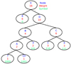 |
Fig. A.1. Full Huffman tree of the example data given in Eq. (A.1). |
| In the text | |
Current usage metrics show cumulative count of Article Views (full-text article views including HTML views, PDF and ePub downloads, according to the available data) and Abstracts Views on Vision4Press platform.
Data correspond to usage on the plateform after 2015. The current usage metrics is available 48-96 hours after online publication and is updated daily on week days.
Initial download of the metrics may take a while.