| Issue |
A&A
Volume 675, July 2023
BeyondPlanck: end-to-end Bayesian analysis of Planck LFI
|
|
|---|---|---|
| Article Number | A12 | |
| Number of page(s) | 12 | |
| Section | Cosmology (including clusters of galaxies) | |
| DOI | https://doi.org/10.1051/0004-6361/202244060 | |
| Published online | 28 June 2023 | |
BEYONDPLANCK
XII. Cosmological parameter constraints with end-to-end error propagation
1
Dipartimento di Fisica, Università degli Studi di Milano, Via Celoria, 16, Milano, Italy
e-mail: This email address is being protected from spambots. You need JavaScript enabled to view it.
2
INFN, Sezione di Milano, Via Celoria 16, Milano, Italy
3
Institute of Theoretical Astrophysics, University of Oslo, Blindern, Oslo, Norway
4
INAF-IASF Milano, Via E. Bassini 15, Milano, Italy
5
INAF – Osservatorio Astronomico di Trieste, Via G.B. Tiepolo 11, Trieste, Italy
6
Planetek Hellas, Leoforos Kifisias 44, Marousi, 151 25
Greece
7
Department of Astrophysical Sciences, Princeton University, Princeton, NJ, 08544
USA
8
Jet Propulsion Laboratory, California Institute of Technology, 4800 Oak Grove Drive, Pasadena, CA, USA
9
Department of Physics, Gustaf Hällströmin katu 2, University of Helsinki, Helsinki, Finland
10
Helsinki Institute of Physics, Gustaf Hällströmin katu 2, University of Helsinki, Helsinki, Finland
11
Computational Cosmology Center, Lawrence Berkeley National Laboratory, Berkeley, CA, USA
12
Haverford College Astronomy Department, 370 Lancaster Avenue, Haverford, Pennsylvania, USA
13
Max-Planck-Institut für Astrophysik, Karl-Schwarzschild-Str. 1, 85741 Garching, Germany
14
Dipartimento di Fisica, Università degli Studi di Trieste, Via A. Valerio 2, Trieste, Italy
Received:
20
May
2022
Accepted:
20
September
2022
Abstract
We present cosmological parameter constraints estimated using the Bayesian BEYONDPLANCK analysis framework. This method supports seamless end-to-end error propagation from raw time-ordered data onto final cosmological parameters. As a first demonstration of the method, we analyzed time-ordered Planck LFI observations, combined with selected external data (WMAP 33–61 GHz, Planck HFI DR4 353 and 857 GHz, and Haslam 408 MHz) in the form of pixelized maps that are used to break critical astrophysical degeneracies. Overall, all the results are generally in good agreement with previously reported values from Planck 2018 and WMAP, with the largest relative difference for any parameter amounting about 1σ when considering only temperature multipoles between 30 ≤ ℓ ≤ 600. In cases where there are differences, we note that the BEYONDPLANCK results are generally slightly closer to the high-ℓ HFI-dominated Planck 2018 results than previous analyses, suggesting slightly less tension between low and high multipoles. Using low-ℓ polarization information from LFI and WMAP, we find a best-fit value of τ = 0.066 ± 0.013, which is higher than the low value of τ = 0.052 ± 0.008 derived from Planck 2018 and slightly lower than the value of 0.069 ± 0.011 derived from the joint analysis of official LFI and WMAP products. Most importantly, however, we find that the uncertainty derived in the BEYONDPLANCK processing is about 30 % greater than when analyzing the official products, after taking into account the different sky coverage. We argue that this uncertainty is due to a marginalization over a more complete model of instrumental and astrophysical parameters, which results in more reliable and more rigorously defined uncertainties. We find that about 2000 Monte Carlo samples are required to achieve a robust convergence for a low-resolution cosmic microwave background (CMB) covariance matrix with 225 independent modes, and producing these samples takes about eight weeks on a modest computing cluster with 256 cores.
Key words: cosmic background radiation / cosmological parameters / cosmology: observations
© The Authors 2023
 Open Access article, published by EDP Sciences, under the terms of the Creative Commons Attribution License (https://creativecommons.org/licenses/by/4.0), which permits unrestricted use, distribution, and reproduction in any medium, provided the original work is properly cited.
This article is published in open access under the Subscribe to Open model. This email address is being protected from spambots. You need JavaScript enabled to view it. to support open access publication.
1. Introduction
The cosmic microwave background (CMB) represents one of the most powerful probes of cosmology available today, as small variations in the intensity and polarization of this radiation impose strong constraints on cosmological structure formation processes in the early Universe. The first discovery of these fluctuations is attributed to Smoot et al. (1992) and over the past three decades, massive efforts have been undertaken to produce detailed maps with steadily increasing sensitivity and precision (e.g., Bennett et al. 2013; de Bernardis et al. 2000; Louis et al. 2017; Sievers et al. 2013; Ogburn et al. 2010; Planck Collaboration I 2020, and references therein). These measurements have led to a spectacularly successful cosmological concordance model called ΛCDM that posits the universe was created during a hot Big Bang event taking place about 13.8 byr ago; along with the postulate that it was seeded by Gaussian random density fluctuations during a brief period of exponential expansion called inflation and that it consists of about 5% baryonic matter, 30% dark matter, and 65% dark energy. This model is able to describe a host of cosmological observables with exquisite precision (see e.g. Planck Collaboration VI 2020), even though it leaves much to be desired in terms of the theoretical understanding. Indeed, some of the biggest questions in modern cosmology revolve around our understanding of the physical nature of inflation, dark matter, and dark energy, with enormous sums of money spent on attempts to answer these questions. In all these studies, CMB observations play a key role.
The current state-of-the-art, in terms of full-sky CMB observations, is defined by ESA’s Planck satellite mission (Planck Collaboration I 2014, 2016, 2020), which observed the microwave sky in nine frequencies, ranging from 30 to 857 GHz, between 2009 and 2013. These measurements have imposed strong constraints on the ΛCDM model, combining information from temperature and polarization CMB maps with novel gravitational lensing reconstructions (Planck Collaboration VI 2020). While the Planck instrument stopped collecting data in 2013, the final official Planck data release took place as recently as 2020 (Planck Collaboration Int. LVII 2020), clearly testifying to the significant analytical challenges associated with these types of data. Large-scale polarization reconstruction represents a particularly difficult problem, and massive efforts have been undertaken in the aim to control all significant systematic uncertainties (e.g., Planck Collaboration Int. LVII 2020; Delouis et al. 2019).
The next major scientific endeavor for the CMB community is the search for primordial gravitational waves created during the inflationary epoch (e.g., Kamionkowski & Kovetz 2016). Current theories predict that such gravitational waves should imprint large-scale B-mode polarization in the CMB anisotropies, with a map-domain amplitude no larger than a few tens of nanokelvin on degree angular scales. Detecting such a faint signal requires at least one or two orders of magnitude higher sensitivity than Planck, as well as correspondingly more stringent systematics suppression and uncertainty assessment.
The main operational goal of the BEYONDPLANCK project (BeyondPlanck Collaboration 2023) is to translate some of the main lessons learned from Planck in terms of systematics mitigation into practical computer code that can be used for next-generation B-mode experiment analysis. And among the most important lessons learned in this respect from Planck regards the tight connection between instrument characterization and astrophysical component separation. Because any CMB satellite experiment must, in practice, be calibrated with in-flight observations of astrophysical sources, the calibration is limited by our knowledge of the astrophysical sources in question – and this must itself be derived from the same data set. Instrument calibration and component separation must therefore be performed jointly, and a non-negligible fraction of the full uncertainty budget arises from degeneracies between the two.
The BEYONDPLANCK project addresses this challenge by constructing a complete end-to-end analysis pipeline for CMB observation into one integrated framework that does not require intermediate human intervention. This is the first complete approach to support seamless end-to-end error propagation for CMB applications, including full marginalization over both instrumental and astrophysical uncertainties and their internal degeneracies. We refer to BeyondPlanck Collaboration (2023), Colombo et al. (2023) for further discussion.
For pragmatic reasons, the current BEYONDPLANCK pipeline has so far only been applied to the Planck LFI observations, which have significantly lower signal-to-noise ratios (S/N) than the Planck HFI observations. The cosmological parameter constraints derived in the following are therefore not in and of themselves competitive in terms of absolute uncertainties, as compared with already published Planck constraints. Rather, the present analysis focuses primarily on general algorithmic aspects, and represents a first real-world demonstration of the end-to-end Bayesian framework that will serve as a platform for further development and data integration of different experiments (Gerakakis et al., in prep.).
Noting the sensitivity of large-scale polarization reconstruction to systematic uncertainties, we adopted the reionization optical depth τ as a particularly important probe of stability and performance of the BEYONDPLANCK framework and we aimed to estimate P(τ ∣ d) from Planck LFI and WMAP observations. We also constrained a basic six-parameter ΛCDM model, combining the BEYONDPLANCK low-ℓ likelihood with a high-ℓ Blackwell-Rao CMB temperature likelihood that, for the first time, covers the two first acoustic peaks, or ℓ ≤ 600. Eventually, we also complement this with the Planck high-ℓ likelihood to extend the multipole range to the full Planck resolution, as well as with selected external non-CMB data sets.
The structure of the rest of the paper is as follows: In Sect. 2, we review the global BEYONDPLANCK data model, posterior distribution, and the CMB likelihood, focusing, in particular, on how cosmological parameters are constrained in this framework. In Sect. 3, we present ΛCDM parameter constraints from BEYONDPLANCK alone and combined with the Planck high-ℓ likelihood. In Sect. 4, we assess the impact of systematic uncertainties, adopting τ as a reference parameter. In Sect. 5, we provide an assessment of the Monte Carlo convergence of CMB samples. Finally, we summarize our main conclusions in Sect. 6.
2. Cosmological parameters and BEYONDPLANCK
We start by introducing the global BEYONDPLANCK data model in order to show how it couples to cosmological parameters through the Gibbs loop; for a detailed discussion, we refer to BeyondPlanck Collaboration (2023) and references therein. Explicitly, the BEYONDPLANCK time-ordered data model is expressed as:
![Mathematical equation: $$ \begin{aligned} \begin{aligned} d_{j,t}&= g_{j,t}\mathsf{P }_{tp,j}\left[ {\mathsf{B }}_{pp^\prime ,j}^{\mathrm{symm} } \sum _c {\mathsf{M }}_{jc}\left(\beta _{p^\prime },\Delta _{bp}^j\right) a_{p^\prime }^c +{\mathsf{B }}_{pp^\prime ,j}^{\mathrm{asymm} } \left(s_{j,t}^{\mathrm{orb} }+s_{j,{ y}}^{\mathrm{fsl} }\right)\right] + \\&\quad + s_{j,t}^{\mathrm{1Hz} } + n_{j,t}^{\mathrm{corr} }+n_{j,t}^{\mathrm{w} }, \end{aligned} \end{aligned} $$](/articles/aa/full_html/2023/07/aa44060-22/aa44060-22-eq1.gif) (1)
(1)
where j indicates radiometer; t and p denotes time sample and pixel on the sky, respectively; and c refers to a given astrophysical signal component. Further, dj, t denotes the measured data value in units of V; gj, t denotes the instrumental gain in units of  ; Ptp, j is the NTOD × 3Npix pointing matrix, where ψ is the polarization angle of the respective detector with respect to the local meridian; Bpp′,j denotes beam convolution;
  denotes element (j, c) of an Ndet × Ncomp mixing matrix, describing the amplitude of the component c, as seen by radiometer j relative to some reference frequency j0;
  is the amplitude of component c in pixel p, measured at the same reference frequency as the mixing matrix M, and expressed in brightness temperature units;
  is the orbital CMB dipole signal in units of Kcmb, including relativistic quadrupole corrections;
  denotes the contribution from far sidelobes, also in units of Kcmb;
  accounts for electronic interference with a 1 Hz period;
  denotes correlated instrumental noise; and
  is uncorrelated (white) noise. The free parameters in this equation are {g, Δbp, ncorr, ac, β}. All the other quantities are either provided as intrinsic parts of the original data sets, or given as a deterministic function of already available parameters.
In addition to the parameters explicitly defined by Eq. (1), we include a set of hyperparameters for each free stochastic random field in the model. For instance, for the CMB component map, aCMB, we define a covariance matrix S, which is taken to be isotropic. Expanding ap = ∑ℓmaℓmYℓ(p) into spherical harmonics, its covariance matrix may be written as:
 (2)
(2)
where Cℓ is called the angular power spectrum. This function is itself a stochastic field to be included in the model and fitted to the data, and, indeed, the angular CMB power spectrum is one of the most important scientific targets in the entire analysis. We note that this spectral-domain covariance matrix approach does not apply solely to astrophysical components, but also to instrumental stochastic fields, such as correlated noise (Ihle et al. 2023) and time-dependent gain fluctuations (Gjerløw et al. 2023).
In many cases, the power spectrum may be further modelled in terms of a smaller set of free parameters, ξ, defined through some deterministic function, Cℓ(ξ). For the CMB case, ξ is nothing but the set of cosmological parameters, and the function Cℓ(ξ) is evaluated using a standard cosmological Boltzmann solver, as implemented, for instance, in the CAMB code (Lewis et al. 2000). If we now define the full set of free parameters in the data model as ω ≡ {g, Δbp, ncorr, ac, β, Cℓ(ξ)}, the goal of the current paper is to derive an estimate of the cosmological parameter posterior distribution P(ξ ∣ d), marginalized over all relevant astrophysical and instrumental parameters. In practice, this marginalization is performed by first mapping the full joint posterior, P(ω ∣ d), as a function of Cℓ through Monte Carlo sampling, then deriving a Cℓ-based CMB power spectrum likelihood from the resulting power spectrum samples, and finally mapping out this likelihood with respect to cosmological parameters using the well-established CosmoMC (Lewis & Bridle 2002) code. We describe in Table 1 the cosmological parameters included in our analysis. The rest of this section details the steps involved in establishing the CMB likelihood for this step.
Overview of cosmological parameters considered in this analysis in terms of mathematical symbol, prior range, and short description (see text for details).
2.1. BEYONDPLANCK posterior distribution and Gibbs sampler
In order to sample from the full global posterior, P(ω ∣ d), we start with Bayes’ theorem:
 (3)
(3)
where P(d ∣ ω)≡ℒ(ω) is called the likelihood, P(ω) is called the prior and P(d) is a normalization factor that is typically referred as the “evidence”. Since the latter is independent of ω, we ignore this factor in the following.
The exact form of the likelihood is defined by the data model in Eq. (1), which is given as a linear sum of various components, all of which are specified in terms of our free parameters, ω. The only term that is not deterministically defined by ω is the white noise, nw, but this is instead assumed to be Gaussian distributed with zero mean and covariance Nw. We can therefore write d = stot(ω)+nw, where stot(ω) is the sum of all model components in Eq. (1), irrespective of their origin, and therefore d − stot(ω)∝N(0, Nw), where N(μ, Σ) denotes a multivariate Gaussian distribution with mean μ and covariance Σ. Thus, the likelihood takes the following form:
 (4)
(4)
The priors are less well defined, and the current BEYONDPLANCK processing uses a mixture of algorithmic regularization priors (e.g., enforcing foreground smoothness on small angular scales; Andersen et al. 2023), instrument priors (e.g., Gaussian or log-normal priors on the correlated noise spectral parameters; Ihle et al. 2023), and informative astrophysical priors (e.g., AME and free-free amplitude priors; Andersen et al. 2023; Colombo et al. 2023). A full summary of all active priors is provided in Sect. 8 of BeyondPlanck Collaboration (2023).
To map out this billion-parameter sized joint posterior distribution, we employed Gibbs sampling; that is, rather than drawing samples directly from the joint posterior distribution, P(ω ∣ d), we drew samples iteratively from all respective conditional distributions, partitioned into suitable parameter sets. This sampling scheme may be formally summarized through the following Gibbs chain,
 (5)
(5)
 (6)
(6)
 (7)
(7)
 (8)
(8)
 (9)
(9)
 (10)
(10)
 (11)
(11)
where ← indicates drawing a sample from the distribution on the right-hand side.
Since the main topic of this paper is cosmological parameter estimation, we summarize here only the CMB amplitude and power spectrum sampling steps, as defined by Eqs. (10) and (11), and we refer to BeyondPlanck Collaboration (2023) and references therein for discussions regarding the other steps.
As shown by Jewell et al. (2004), Wandelt et al. (2004), the amplitude distribution P(a ∣ d, ω \ a), i.e. the probability of a given the data d and the all the model parameters except a, is a multivariate Gaussian with a mean given by the so-called Wiener filter and an inverse covariance matrix given by S(Cℓ)−1 + N−1, where S(Cℓ) and N are, thus, the total effective signal and noise covariance matrices, respectively. Samples from this distribution may be drawn by solving the following system of linear equations, typically using the Conjugate Gradient method (Shewchuk 1994):
 (12)
(12)
In this expression, Mν is called the mixing matrix, and encodes the instrument-convolved spectral energy densities of each astrophysical foreground component, and the ηi results are independent random Gaussian vectors of N(0, 1) variates. For further details on solving this equation, see Eriksen et al. (2008), Seljebotn et al. (2019), BeyondPlanck Collaboration (2023), Colombo et al. (2023).
Sampling from P(Cℓ ∣ d, ω \ Cℓ) is much simpler, as this is an inverse gamma distribution with 2ℓ+1 degrees of freedom for CMB temperature measurements (Wandelt et al. 2004) and a corresponding Wishart distribution for CMB polarization (Larson et al. 2007). The standard sampling algorithm for the former of these is simply to draw 2ℓ−1 random variates from a standard Gaussian distribution, ηi ∼ N(0, 1), and set  , where σℓ = ∑|aℓm|2. The generalization to polarization is straightforward.
The above Gibbs algorithm only represents a formal summary of the algorithm and, in practice, we introduced a few important modifications for computational and robustness reasons. The first modification revolves around Galactic plane masking. As shown by Colombo et al. (2023), the BEYONDPLANCK CMB reconstruction is not perfect along the Galactic plane. To prevent these errors from contaminating the CMB power spectrum and cosmological parameters, we therefore applied a fairly large confidence mask for the actual CMB analysis. At the same time, the Galactic plane does contain invaluable information regarding important global instrumental parameters, for instance, the detector bandpasses (Svalheim et al. 2023a), and excluding these data entirely from the analysis would greatly increase the uncertainties on those parameters. For this reason, we ran the analysis in two main stages; we first ran the above algorithm without a Galactic mask and setting  , primarily to estimate the instrumental and astrophysical parameters; this configuration corresponds to estimating the CMB component independently in each pixel without applying any smoothness prior over the full sky. The cost of setting the power spectrum prior to zero is slightly larger pixel uncertainties than in the optimal case, as the CMB field is now allowed to vary almost independently from pixel to pixel. However, this also ensures that any potential modeling errors remain local, and are not spread across the sky.
Then, once this main sampling process is done, we resampled the original chains with respect to the CMB component by looping through each main sample, fixing all instrumental and (most of the) astrophysical parameters, and sampling the CMB-related parameters again (see Colombo et al. 2023, for full details). For the low-resolution CMB polarization estimation, for which our likelihood relies on a dense pixel-pixel covariance matrix, the main goal of this stage is simply to obtain more samples of the same type as above and to reduce the Monte Carlo uncertainty in the noise covariance matrix (Sellentin & Heavens 2016). In this case, we simply drew n additional samples from Eq. (10), fixing both the instrumental and astrophysical parameters, as well as the CMB aℓm’s for ℓ > 64. We effectively mapped out the local conditional distribution with respect to white noise for each main sample on large angular scales. We conservatively drew n = 50 new samples per main sample in this step, but after the analysis started, we checked that a set of as few as ten subsamples achieves an equivalent effect. On the other hand, since the cost of producing one of these subsamples is almost two orders of magnitude smaller than producing a full sample, this additional cost is negligible.
This approach is not suitable for a high-resolution CMB temperature analysis, since we cannot construct a pixel-pixel covariance matrix with millions of pixels. In this case, we used the Gaussianized Blackwell-Rao estimator instead (Chu et al. 2005; Rudjord et al. 2009), which was also used for CMB temperature analysis up to ℓ ≤ 30 by Planck (e.g., Planck Collaboration V 2020). This estimator relies on proper Cℓ samples and we therefore resampled the main chains once again, but this time we applied the confidence mask and enable the Cℓ sampling step; once again, all instrumental and (most of) the astrophysical parameters are fixed at their main chain sample values. Thus, this step includes solving Eq. (12) with an inverse noise covariance matrix that is zero in the masked pixels and a non-local S covariance matrix, and this translates into a very high condition number for the coefficient matrix on the left-hand side (Seljebotn et al. 2019). In fact, the computational cost of a single CMB temperature power spectrum sample is comparable to the cost of a full main sample, and we therefore only produce 4000 of these. Fortunately, as shown in Sect. 5, this is sufficient to achieve good convergence up to ℓ ≲ 700. However, it does not allow us to explore the low signal-to-noise regime above ℓ ⪆ 800. For this reason, we conservatively limited the current BEYONDPLANCK temperature analysis to ℓ ≤ 600, leaving some buffer, and combined it with Planck 2018 results at higher multipoles when necessary.
2.2. BEYONDPLANCK CMB likelihood
The BEYONDPLANCK CMB power spectrum likelihood is based on two well-established techniques, namely, brute-force low-resolution likelihood evaluation on large angular scales for polarization (e.g., Page et al. 2007; Planck Collaboration V 2020) and a Blackwell-Rao (BR) estimation for intermediate angular scales for temperature (Chu et al. 2005; Rudjord et al. 2009; Planck Collaboration XI 2016). The main variations are that we employed the signal-to-noise eigenmode compression technique described by Tegmark et al. (1997), Gjerløw et al. (2015) for the low-resolution likelihood (to reduce the dimensionality of the covariance matrix and, thus, the number of Gibbs samples required for convergence); in addition, we were thus able to use the BR estimator to ℓ ≤ 600, not only ℓ ≤ 200, as was done in Planck 2018; the main reason for this is that in the current scheme the CMB sky map samples are drawn from foreground-subtracted frequency maps (30, 44, 70 GHz...), each with a well-defined white noise term, while in the Planck analysis they were generated from component-separated CMB maps (Commander, NILC, SEVEM, and SMICA; Planck Collaboration IV 2020) with smoothed white noise terms. In this section, we briefly review the mathematical backgrounds for each of these two likelihood approximations and we refer to the aforementioned papers for further details.
2.2.1. Low-ℓ temperature+polarization likelihood
Starting with the low-resolution case, the appropriate expression for a multivariate Gaussian likelihood is expressed as:
 (13)
(13)
where  represents a CMB-plus-noise map and N is its corresponding effective noise covariance map. This expression has formed the basis of numerous exact CMB likelihood codes, going at least as far back as COBE-DMR (e.g., Gorski 1994).
The key novel aspect of the current analysis is simply how to establish  and N; in previous analyses,
  has typically been estimated by maximum-likelihood techniques, while N has been estimated through analytic evaluations that are only able to take into account a rather limited set of uncertainties, such as white and correlated noise, a very simplified template-based foreground model, and simple instrumental models of modes that have poorly measured gains as a consequence of the scanning strategy. In contrast, in the current paper, both these quantities are estimated simply by averaging over all available Gibbs samples:
 (14)
(14)
 (15)
(15)
where brackets indicate Monte Carlo averages. Thus, in this approach, there is no need to explicitly account for each individual source of systematic effects in the covariance matrix, but they are all naturally and seamlessly accounted for through the Markov chain samples.
The main challenge associated with this approach is related to how many samples are required for N to actually converge. As discussed by Sellentin & Heavens (2016), a general requirement is for nsamp ≫ nmode, where nsamp is the number of Monte Carlo samples and nmode is the number of modes in the covariance matrix. To establish a robust covariance matrix, one may therefore either increase nsamp (at the cost of increased computational costs) or decrease nmode (at the cost of increased final uncertainties). It is therefore of great interest to compress the relevant information in  into a minimal set of modes that capture as much of the relevant information as possible. In our case, the main cosmological target for the low-resolution likelihood is the optical depth of reionization, τ, and the main impact of this parameter on the Cℓ power spectrum for Planck LFI happens in polarization at very low multipoles, ℓ ≲ 6 − 8, due to the limited sensitivity of the instrument (Planck Collaboration V 2020).
In practice, we compressed the information using the methodology discussed by Tegmark et al. (1997), which isolates the useful modes through Karhunen-Loève (i.e., signal-to-noise eigenmode) compression. Adopting the notation introduced by Gjerløw et al. (2015), we transform the data into a convenient basis through a linear operator of the form  , where the projection operator is defined as:
![Mathematical equation: $$ \begin{aligned} \mathsf P = [\mathsf P _h\left( \mathsf S ^{1/2}\mathsf{N }^{-1}\mathsf S ^{1/2} \right)\mathsf P _h^t]_\epsilon \mathsf{M }. \end{aligned} $$](/articles/aa/full_html/2023/07/aa44060-22/aa44060-22-eq31.gif) (16)
(16)
Here, Ph is an harmonic space truncation operator that retains only spherical harmonics up to a truncation multipole ℓt, M is a masking operator, and [A]ϵ is the set of eigenvectors of A with a fractional eigenvalue larger than a threshold value ϵ. Thus, P corresponds to a orthonormal basis on the masked sky that retains primarily multipoles below ℓt1, and with a relative S/N higher than ϵ. It is important to note that this projection operator results in an unbiased likelihood estimator irrespective of the specific values chosen for ℓt and ϵ, and the only cost of choosing restrictive values for either is just larger uncertainties in the final results. This is fully equivalent to masking pixels on the sky; as long as the mask definition does not exploit information in the CMB map itself, no choice of mask can bias the final results, but only modify the final error bars. In this paper, we adopt a multipole threshold of ℓmax = 8 and a signal-to-noise threshold of 10−6; we apply the R1.8 analysis mask defined by Planck Collaboration V (2020; with fsky = 0.68); and we use the best-fit Planck 2018 ΛCDM spectrum to evaluate S. In total, this leaves 225 modes in P. Determining how many Monte Carlo samples are required to robustly map out the likelihood for this number of modes is one of the key results presented in Sect. 4.
2.2.2. High-ℓ temperature likelihood
For the high-ℓ temperature analysis, we exploited the Blackwell-Rao (BR) estimator (Chu et al. 2005), which has been demonstrated to work very well for high S/N data (Eriksen et al. 2004). This is the case for the BEYONDPLANCK temperature power spectrum below ℓ ≲ 700, whereas the S/N for high-ℓ polarization is very low everywhere, even when combining LFI and WMAP data.
In practice, we employed the Gaussianized Blackwell-Rao estimator (GBR), as presented in Rudjord et al. (2009) and used by Planck (Planck Collaboration V 2020), in order to reduce the number of samples required to achieve good convergence at high multipoles. In this approach, the classical Blackwell-Rao estimator is first used to estimate the univariate Cℓ likelihood for each multipole separately:
 (17)
(17)
where  is the observed power spectrum of the i’th Gibbs sample CMB sky map, sCMB. This distribution is used to define a Gaussianizing change-of-variables, xℓ(Cℓ), multipole-by-multipole by matching differential quantiles between the observed likelihood function and a standard Gaussian distribution. The final likelihood expression may then be evaluated as follows:
 (18)
(18)
where x = {xℓ(Cℓ)} is the vector of transformed input power spectrum coefficients; ∂Cℓ/∂xℓ is the Jacobian of the transformation; and the mean μ = {μℓ} and covariance matrix Cℓℓ′ = ⟨(xℓ − μℓ)(xℓ′ − μℓ′)⟩ are estimated from the Monte Carlo samples after Gaussianization with the same change of variables. This expression is by construction exact for the full-sky and uniform noise case, due to the diagonal form of the noise covariance matrix, and consequently the full expression factorizes in ℓ. For real-world analyses that include sky cuts, anisotropic noise, and systematic uncertainties, it is strictly speaking an approximation; however, as shown by Rudjord et al. (2009), it is an excellent approximation even for relatively large sky cuts. Furthermore, any differences induced by additional instrumental systematic error propagation are small compared to the effect of the Galactic mask, which totally dominates the sample variance component of the high-ℓ temperature likelihood. In this paper, we derived ΛCDM cosmological parameters using the Gaussianized GBR estimator using the multipole range 9 ≤ ℓ ≤ 600. Additional details can be found in BeyondPlanck Collaboration (2023) and Colombo et al. (2023).
2.3. CAMB and CosmoMC
The final cosmological parameters were sampled with CosmoMC (Lewis & Bridle 2002), using the above likelihoods as inputs. This code implements a Metropolis-Hastings algorithm to efficiently probe the whole parameter space, using various speed-up and tuning methods (Neal 2005; Lewis 2013). In our analysis, we ran eight chains until they reach convergence, as defined by a Gelman-Rubin statistic of R − 1 < 0.01 (Gelman & Rubin 1992), while discarding the first 30 % of each chain as burn-in. This is due to the way CosmoMC learns an accurate orthogonalization and proposal distribution for the parameters from the sample covariance of the previous samples. In general, quoted error bars correspond to 68 % confidence ranges, except in cases for which a given parameter is consistent with a hard prior boundary (such as the tensor-to-scalar ratio, r), in the case of which we report upper 95 % confidence limits.
3. Six-parameter ΛCDM constraints
At this point, we are ready to present standard ΛCDM cosmological parameter constraints as derived from the BEYONDPLANCK likelihood and we compare them with previous estimates from Planck 2018 (Planck Collaboration VI 2020). The main results are shown in Fig. 1 in terms of one- and two-dimensional marginal posterior distributions of the six ΛCDM base parameters for three different cases. The blue contours show results derived from BEYONDPLANCK alone, using only the temperature information up to ℓ ≤ 600 and polarization information between 2 ≤ ℓ ≤ 8, while red contours show corresponding results when the temperature multipole range is extended with the Planck 2018 TT likelihood2 between 601 ≤ ℓ ≤ 2500. Finally, the green contours show the full Planck 2018 (TT + lowE) posterior distributions. The BEYONDPLANCK results are summarized in terms of posterior means and standard deviations in Table 2, where we also report constraints when including CMB lensing and baryonic acoustic oscillations (BAO). We refer to Planck Collaboration XVI (2014) and Planck Collaboration XIII (2016) for corresponding Planck analyses.
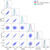 |
Fig. 1. Constraints on the six ΛCDM parameters from the BEYONDPLANCK likelihood (blue contours) using the low-ℓ brute-force temperature-plus-polarization likelihood for ℓ ≤ 8 and the high-ℓ Blackwell-Rao likelihood for 9 ≤ ℓ ≤ 600. The red contours show corresponding constraints when adding the high-ℓ Planck 2018 TT-only likelihood for 601 ≤ ℓ ≤ 2500, while green contours show the same for the Planck 2018 likelihood. |
Constraints on the six ΛCDM base parameters with confidence intervals at 68% from CMB data alone and adding lensing + BAO.
The combined BEYONDPLANCK + Planck 2018 likelihood presented in this paper is the direct sum of the two log-Posteriors. In general, this procedure may be affected by ℓ-to-ℓ correlations arising from masking, noise, systematic effects, and foreground residuals. Assessing the impact of such correlations on the final parameter estimates is not a trivial procedure, as it typically requires joint simulations of Planck LFI and HFI observations (in addition to any necessary external dataset) that are to be analyzed in the same manner as the actual data. However, we can look at the mode coupling within each individual dataset to have an insight on the level of correlation between the two parts of the joint likelihood. Around ℓ = 600, BEYONDPLANCKCℓ values show a correlation level of few percent between the nearest and next-to-nearest multipoles, rapidly falling off for more distant modes. In the same multipole range, the Planck 2018 likelihood shows correlation between nearby bins of order 0.001% for 100 and 143 GHz and 0.1% for 143x217 and 217 GHz. These estimates include contributions from all the possible sources of correlations mentioned above. However, noise and systematics effects are largely uncorrelated between LFI and HFI measurements. In addition, BEYONDPLANCK CMB map is largely dominated by 44 and 70 GHz measurements, while Planck 2018 likelihood is based on HFI measurements at 100, 143, and 217 GHz. We expect residual foreground contamination at these frequency ranges to be dominated by different astrophysical sources and to be be only weakly correlated between the two likelihoods. Finally, BEYONDPLANCK confidence mask is different from Planck mask, corresponding to a different pattern of residual multipole coupling. Therefore, we expect correlations between the two parts of the likelihood to be significantly smaller than those within a single dataset. This same argument has been explored in Gjerløw et al. (2013) by showing the impact of multipole correlation at ℓ = 30, which further motivates our choice of uncorrelated likelihoods at ℓ = 600.
Overall, we observe excellent agreement between the various cases, and the most discrepant parameter is the optical depth of reionization, for which the BEYONDPLANCK result (τ = 0.065 ± 0.012) is higher than the Planck 2018 (TT + lowE) constraint (τ = 0.052 ± 0.008) by roughly 1σ. In turn, this also translates into a higher initial amplitude of scalar perturbations, As, by about 1.5σ. At the same time, it is important to note that the high-ℓ information from the HFI-dominated Planck 2018, likelihood plays a key role in constraining all parameters (except τ), by reducing the width of each marginal distribution by a factor of typically 5–10. As such, the good agreement seen in Fig. 1 is not surprising, but rather expected from the high level of correlations between the input datasets.
It is therefore interesting to assess agreement between the various likelihood using directly comparable datasets, and such a comparison is shown in Fig. 2. In this case, we show constraints derived using only TT information between 30 ≤ ℓ ≤ 600, combined with a Gaussian prior of τ = 0.060 ± 0.015. The solid lines show results for BEYONDPLANCK (black), Planck 2018 (blue), and WMAP (red), respectively, while the dashed-dotted green line for reference shows the same Planck 2018 constraints as in Fig. 1 derived from the full likelihood.
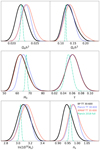 |
Fig. 2. Comparison between ΛCDM parameters derived using TT-only between 30 ≤ ℓ ≤ 600 for BEYONDPLANCK (black), Planck 2018 (blue), and WMAP (red). All these cases include a Gaussian prior of τ = 0.06 ± 0.015. For comparison, the full Planck 2018 estimates are shown as dot-dashed green distributions. |
Taken at face value, the agreement between the three datasets appears reasonable in this directly comparable regime, as the most discrepant parameters are Ωbh2 and H0, which both differ by about 1σ between BEYONDPLANCK and Planck 2018 and WMAP. However, it is important to note that all three of these datasets are nominally cosmic variance limited in the multipole range between 30 ≤ ℓ ≤ 600, and therefore we should, in principle, expect a perfect agreement between these distributions and that is obviously not the case. Some of these discrepancies can be explained in terms of different masking, noting that the effective sky fraction of the BEYONDPLANCK, Planck 2018, and WMAP likelihoods are about 63, 65, and 75%, respectively. However, as shown by Planck Collaboration V (2020), such small variations are not individually large enough to move the main cosmological parameters by as much as 1σ.
It is therefore likely the actual data processing pipelines used to model and propagate astrophysical and instrumental systematic errors play a significant role in explaining these differences. In this respect, we make two interesting observations. First of all, we note that BEYONDPLANCK pipeline fundamentally differs from the two previous pipelines from a statistical point of view, as it is the first pipeline to implement true end-to-end Bayesian modeling that propagate all sources of astrophysical and instrumental systematic uncertainties to the final cosmological parameters; in comparison, the other two pipelines both rely on a mixture of frequentist and Bayesian techniques that are only able to propagate a subset of all uncertainties. Second, we note that the low-ℓ LFI-dominated BEYONDPLANCK results are for several parameters more consistent with the high-ℓ HFI-dominated Planck 2018 results than the two previous pipelines; specifically, this is the case for Ωbh2, Ωch2, and As, while for H0, the Planck 2018 low-ℓ likelihood is slightly closer to its high-ℓ results, while BEYONDPLANCK and WMAP are identical. Finally, for ns all three pipelines result in comparable agreement with the high-ℓ result in terms of absolute discrepancy, but with a different sign; BEYONDPLANCK prefers a stronger tilt than either Planck 2018 or WMAP. All in all, we conclude that there seems to be slightly less internal tension between low and high multipoles when using the BEYONDPLANCK likelihood. Still, the main conclusion from this analysis is that all these differences are indeed small in an absolute sense, and subtle differences at the 1σ level for 30 ≤ ℓ ≤ 600 do not represent a major challenge for the overall cosmological parameters derived from the full Planck 2018 data, as explicitly shown in Fig. 1.
Before concluding this section, we comment on two important cosmological parameters that have been the focus of particularly intense discussion after the Planck 2018 release, namely the Hubble expansion parameter, H0, and the RMS amplitude of scalar density fluctuations, σ8. Figure 3 shows two-dimensional marginal distributions for H0–Ωm and σ8–Ωm, respectively, for various data combinations. Here, we see that BEYONDPLANCK on its own is not able to shed new light on the either of the two controversies, due to its limited angular range. When used in combination with high-ℓ Planck 2018 information, however, we see that BEYONDPLANCK prefers an even slightly lower mean value of H0 than Planck 2018, although also with a slightly larger uncertainty. The net discrepancy with respect to Riess et al. (2018) is, thus, effectively unchanged.
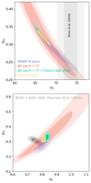 |
Fig. 3. 2D marginal posterior distributions for the parameter pairs H0–Ωm (top) and σ8–Ωm (bottom) as computed with the BEYONDPLANCK-only likelihood (red); the BEYONDPLANCK likelihood extended with the Planck 2018 high-ℓ TT likelihood (green); the full Planck 2018 likelihood (yellow); the WMAP likelihood (blue); and, for the bottom figure, the joint cosmic shear and galaxy clustering likelihood from KiDS-1000 and BOSS (Heymans et al. 2021, gray). |
The same observation holds for σ8, for which BEYONDPLANCK prefers a higher mean value than Planck, increasing the absolute discrepancy with cosmic shear and galaxy clustering measurements from Heymans et al. (2021). In this case, we see that BEYONDPLANCK prefers an even higher value than Planck, by about 1.5σ, further increasing the previously reported tension with late-time measurements. This difference with respect to Planck is driven by the higher value of τ, as already noted in Fig. 1.
4. Large-scale polarization and the optical depth of reionization
As discussed by BeyondPlanck Collaboration (2023), the main purpose of the BEYONDPLANCK project has not been to derive new state-of-the-art ΛCDM parameter constraints, for which (as we explain above) Planck HFI data are essential. Rather, the main motivation behind this work was to develop a novel and statistically consistent Bayesian end-to-end analysis framework for past, current, and future CMB experiments, with a particular focus on next-generation polarization experiments. As such, the single most important scientific target in all of this work is the optical depth of reionization, τ, which serves as an overall probe of the efficiency of the entire framework. At this point, we are finally ready to present the main results regarding this parameter, as given below.
In the left panel of Fig. 4, we show the marginal posterior distribution for τ as derived from the low-ℓ BEYONDPLANCK likelihood alone (black curve) and compare this result with the corresponding estimates from the literature (Hinshaw et al. 2013; Planck Collaboration VI 2020; Natale et al. 2020; Pagano et al. 2020). We note, however, that making head-to-head comparisons between all of these is non-trivial, as the reported parameters depend on different assumptions and data combinations. For example, Pagano et al. (2020) considers a likelihood that includes Commander 2018 temperature likelihood and low-ℓ E modes and marginalizes over As, whereas Natale et al. (2020) considers only low-ℓ polarization and marginalizes over only a small set of strongly correlated parameters, that is, As and/or r. Taking into account the fact that Natale et al. (2020) analyzed the official LFI and WMAP products jointly, we chose to tune our analysis configuration to their findings to facilitate a head-to-head comparison for the most relevant case. The corresponding numerical values are summarized in Table 3.
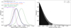 |
Fig. 4. Comparison of marginal posterior distributions of the reionization optical depth from Planck 2018, shown on the left (red, dotted; Planck Collaboration VI 2020), 9-yr WMAP (green, dot-dashed; Hinshaw et al. 2013), Planck DR4 (cyan, dotted; Tristram et al. 2022), Planck HFI (purple, dot-dashed; Pagano et al. 2020), WMAP Ka–V and LFI 70 GHz (fitting τ + As; Natale et al. 2020; blue, dashed); and BEYONDPLANCK using multipoles ℓ = 2–8, marginalized over the scalar amplitude As (black). Corresponding marginal BEYONDPLANCK tensor-to-scalar ratio posteriors derived using BB multipoles between ℓ = 2–8, marginalized over the scalar amplitude As (gray), and by fixing all the ΛCDM parameters to their best-fit values, shown on the right (black). The filled region corresponds to the 95% confidence interval. |
We see that the BEYONDPLANCK polarization-only estimate is in reasonable agreement with the Natale et al. result based on the official LFI and WMAP products, with an overall shift of about 0.2σ. However, there are two important differences to note in this regard. First, the BEYONDPLANCK mean value is slightly lower than the LFI+WMAP value and it is therefore in slightly better agreement with the HFI-dominated results. Second, and more importantly, we see that the BEYONDPLANCK uncertainty is greater for BEYONDPLANCK than LFI+WMAP, despite the fact that its sky fraction is larger (68 versus 54 %). Since the uncertainty on τ scales roughly inversely proportionally with the square root of the sky fraction3, we can make a rough estimate of what our uncertainty should have been for their analysis setup:
 (19)
(19)
 (20)
(20)
For comparison, the actual Natale et al. (2020) uncertainty is 0.011, or about 30% smaller. We interpret our greater uncertainty as being due to marginalizing over a more complete set of statistical uncertainties in the BEYONDPLANCK analysis framework than is possible with the frequentist-style and official LFI and WMAP data products. As such, this comparison directly highlights the importance of the end-to-end approach.
Table 3 also contains several goodness-of-fit and stability tests. Specifically, we first note that the best-fit tensor-to-scalar ratio is consistent with zero and with an upper 95% confidence limit of r < 0.84. While this is by no means competitive with current state-of-the-art constraints from the combination of BICEP2/Keck and Planck of r < 0.032 (Tristram et al. 2022), the absence of strong B-mode power is a confirmation that the BEYONDPLANCK processing seems clean of systematic errors; these results are in good agreement with the power spectrum results presented by Colombo et al. (2023). As done above for τ, we can rescale the upper limit on r to account for the different sky fraction of Natale et al. (2020), leading to a constraint of r < 0.94, which is to be compared with r < 0.79 obtained in that work. This suggests that also for r the marginalization over additional model parameters included in the BEYONDPLANCK framework leads to a ∼20% increase in uncertainty compared to a traditional analysis.
We also note in Table 3 that the impact of ℓ = 2 from the analysis is small, and the only noticeable effect of removing it from the analysis is to increase the uncertainties on τ and r by about 10%. This is important because the BEYONDPLANCK processing is not guaranteed to have a unity transfer function for this single mode (EE, ℓ = 2): As discussed by Gjerløw et al. (2023), there is a strong degeneracy between the CMB polarization quadrupole and the relative gain parameters and the current pipeline breaks this by imposing a ΛCDM prior on the single EE ℓ = 2 mode. Although this effect is explicitly demonstrated through simulations to be small by Brilenkov et al. (2023), it is still comforting to see that this particular mode does not have a significant impact on the final results.
Finally, the sixth column in Table 3 shows the χ2 probability-to-exceed (PTE), where the main quantity is defined as:
 (21)
(21)
For a Gaussian and isotropic random field, this quantity should be distributed according to a  distribution, where ndof = 225 is the number of degrees of freedom, which in our case is equal to the number of basis vectors in
  . The PTE for our likelihood is 0.32, indicating full consistency with the ΛCDM best-fit model4 and sample-based noise covariance matrix.5
Figure 5 shows corresponding results for different sky fractions, adopting the series of analysis masks defined by Planck Collaboration V (2020). The tensor-to-scalar ratio is reported in terms of a nominal detection level in units of σ, as defined by matching the observed likelihood ratio ℒ(rbf)/ℒ(r = 0) with that of a Gaussian standard distribution. Overall, we see that all results are largely insensitive to sky fraction, which suggests that the current processing has managed to remove most statistically significant astrophysical contamination (Andersen et al. 2023; Svalheim et al. 2023b). However, we do note that a small B-mode contribution appears at the most aggressive sky coverage of 83%, and also that the χ2 PTE starts to fall somewhat above 68%. For this reason, we conservatively adopted a sky fraction of 68% for our main results, but we note that 73% would have been equally well justified.
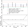 |
Fig. 5. Low-ℓ likelihood stability as a function of sky fraction. All results are evaluated adopting the same series of LFI processing masks as defined by Planck Collaboration V (2020). From top to bottom, the three panels show (1) posterior τ estimate; (2) posterior r estimate, expressed in terms of a detection level with respect to a signal with vanishing B-modes in units of σ; and (3) χ2 PTE evaluated for the best-fit power spectrum in each case. |
Summary of cosmological parameters dominated by large-scale polarization and goodness-of-fit statistics.
Before concluding this section, we return to the importance of end-to-end error propagation, performing a simple analysis in which we estimate the marginal τ posterior under three different regimes of systematic error propagation. In the first regime, we assume that the derived CMB sky map is entirely free of both astrophysical and instrumental uncertainties and the only source of uncertainty is white noise. This case is evaluated by selecting one random CMB sky map sample as the fiducial sky and we do not marginalize over instrumental or astrophysical samples when evaluating the sky map and noise covariance matrix in Eq. (15). In the second regime, we assume that the instrumental model is perfectly known, while the astrophysical model is uncertain. In the third and final regime, we assume that both the instrumental and astrophysical parameters are uncertain and we marginalize over all of them, as in the main BEYONDPLANCK analysis. The results from these calculations are summarized in Fig. 6. As expected, we see that the uncertainties increase when marginalizing over additional parameters. Specifically, the uncertainty of the fully marginalized case is 46% larger than for white noise, and 32% larger than the case marginalizing over the full astrophysical model. This calculation further emphasizes the importance of global end-to-end analysis that takes jointly into account all sources of uncertainty.
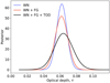 |
Fig. 6. Estimates of τ under different uncertainty assumptions. The blue curve shows marginalization over white noise only; the red curve shows marginalization over white noise and astrophysical uncertainties; and, finally, the black curve shows marginalization over all contributions, including low-level instrumental uncertainties, as in the final BEYONDPLANCK analysis. |
5. Monte Carlo convergence
As noted in Sect. 2, one important goal of the current paper is to assess how many end-to-end Monte Carlo samples are required to robustly derive covariance matrices and cosmological parameters by Gibbs sampling. This permits us to answer this question quantitatively, using the results presented above.
Starting with the low-ℓ polarization likelihood, we once again adopted τ as a proxy for overall stability, which we show in Fig. 7τ as a function of the number of Gibbs samples, nsamp, used to build the low-ℓ likelihood inputs in Eq. (15)6. Here, we see that the estimates are positively biased for small values of nsamp, with a central value around τ = 0.085. However, the estimates then starts to gradually fall while the Markov chains explore the full distribution. This behavior can be qualitatively understood as follows: the actual posterior mean sky map converges quite quickly with number of samples, and stabilizes only with a few hundred samples. However, the τ estimate is derived by comparing the covariance of this sky map with the predicted noise covariance as given by N; any excess fluctuations in  compared to N is interpreted as a positive S contribution. Convergence in N is obviously much more expensive than convergence in
  , which leads to the slow decrease in τ as a function of sample as N becomes better described by a greater number of samples.
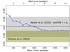 |
Fig. 7. Convergence of constraints of the reionization optical depth as a function of the number of main chain samples used to construct the CMB mean map and covariance matrix and the relative wall time needed to produce such samples in the main Gibbs loop. The solid blue line shows the posterior mean for τ, while the gray and green regions show the corresponding 68% confidence interval for Natale et al. (2020) and Tristram et al. (2022), respectively. |
From Fig. 7, we see that the results stabilize only after nsamp ≈ 2000 main Gibbs samples, which is almost nine times greater than the number of modes in the covariance matrix, nmode = 225. Obviously, this number will depend on the specifics of the data models and datasets in question, and more degenerate models will in general require more samples, but at least this estimate provides a real-world number that may serve as a rule-of-thumb for future analyses.
Finally, to assess convergence for the high-ℓ temperature likelihood, we adopt the Gelman-Rubin (GR) R convergence statistic, which is defined as the ratio of the “between-chain variance” and the “in-chain variance” (Gelman & Rubin 1992). We evaluate this quantity based on the four available σℓ chains, including different numbers of samples in each case, ranging between 250 to 4000. The results from this calculations are summarized in Fig. 8. Here we see that the convergence improves rapidly below ℓ ≲ 600–800, while multipoles above ℓ ≳ 1000 converge very slowly. We adopt a stringent criterion of R − 1 < 0.01 (dashed horizontal line), and conservatively restrict the multipole range used by BEYONDPLANCK to ℓ ≤ 600. With these restrictions, we once again see that about 2000 samples are required to converge.
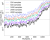 |
Fig. 8. Gelman-Rubin convergence statistic for the BEYONDPLANCK TT angular power spectrum, as evaluated from four independent σℓ chains. A R − 1 value lower than 0.1 typically indicates acceptable convergence. Moreover, we report the R − 1 = 10−2 threshold (dotted black line) representing a safer criterion to assess convergency. |
6. Conclusions
The main motivation behind the BEYONDPLANCK project is to develop a fully Bayesian framework for a global analysis of CMB and related datasets that allows for a joint analysis of both astrophysical and instrumental effects and, thus, a robust end-to-end error propagation. In this paper, we have demonstrated this framework in terms of standard cosmological parameters, which arguably represent the most valuable deliverable for any CMB experiment. We emphasize that this work is primarily algorithmic in nature, and intended to demonstrate the Bayesian framework itself using a well-controlled dataset, namely the Planck LFI measurements; it is not intended to replace the current state-of-the-art Planck 2018 results, which are based on highly sensitive HFI measurements.
With this observation in mind, we find that the cosmological parameters derived from LFI and WMAP in BEYONDPLANCK are overall in good agreement with those published from the previous pipelines. When considering the basic ΛCDM parameters and temperature information between 30 ≤ ℓ ≤ 600, the typical agreement between the various cases is better than 1σ, and we also note that in the cases where there are discrepancies, the BEYONDPLANCK results are typically somewhat closer to the high-ℓ HFI constraints than previous results, indicating less internal tension between low and high multipoles.
Overall, the most noticeable difference is seen for the optical depth of reionization, for which we find a slightly higher value of τ = 0.066 ± 0.013 than Planck 2018 at τ = 0.052 ± 0.008. At the same time, this value is lower than the corresponding LFI-plus-WMAP result derived by Natale et al. (2020) of τ = 0.069 ± 0.011, which suggests that the current processing has cleaned up more systematic errors than in previous LFI processing. Furthermore, and even more critically, we find that the BEYONDPLANCK uncertainty is almost 30% larger than latter when taking into account the different sky fraction. We argue that this is due to BEYONDPLANCK taking into account a much richer systematic error model than previous pipelines. Indeed, this result summarizes the main purpose of the entire BEYONDPLANCK project in terms of one single number. We believe that this type of global end-to-end processing will be critical for future analysis of next-generation B-mode experiments.
A second important goal of the current paper was to quantify how many samples are actually required to converge for a Monte Carlo-based approach. Based on the current analysis, we find that about 2000 end-to-end samples are need to achieve robust results. Clearly, introducing additional sampling steps that more efficiently break down long Markov chain correlation lengths will be important to reduce this number in the future, but already the current results proves that the Bayesian approach is computationally feasible for past and current experiments.
Note that these modes do have some sensitivity to higher multipoles due to non-orthogonality of the spherical harmonics on a masked sky; the quoted truncation limit is therefore only approximate.
We adopt the public Planck 2018 likelihood code (PLC; version 3.0) when extending the BEYONDPLANCK likelihood and including lensing and BAO constraints.
This assumption has been verified by simulating two sets of 1000 CMB plus noise maps, with a different sky coverage, and computing the estimate of τ in order to retrieve the proper uncertainty scaling factor as function of fsky.
In this paper, we denote quantities fixed to a fiducial ΛCDM best-fit value with the superscript bf.
We note that this was not the case in the first preview version of the BEYONDPLANCK results announced in November 2020: In that case the full-sky χ2 PTE was 𝒪(10−4), and this was eventually explained in terms of gain over-smoothing by Gjerløw et al. (2023) and non-1/f correlated noise contributions by Ihle et al. (2023). Both these effects were mitigated in the final BEYONDPLANCK processing, as reported here.
Recall that for each main Gibbs chain sample, we additionally draw n = 50 subsamples to cheaply marginalize over white noise, such that the actual number of individual samples involved in Fig. 7 is actually 50 times higher than what is shown; the important question for this test, however, is the number of main Gibbs samples.
Acknowledgments
We thank Prof. Pedro Ferreira and Dr. Charles Lawrence for useful suggestions, comments and discussions. We also thank the entire Planck and WMAP teams for invaluable support and discussions, and for their dedicated efforts through several decades without which this work would not be possible. The current work has received funding from the European Union’s Horizon 2020 research and innovation program under grant agreement numbers 776282 (COMPET-4; BEYONDPLANCK), 772253 (ERC; BITS2COSMOLOGY), and 819478 (ERC; COSMOGLOBE). In addition, the collaboration acknowledges support from ESA; ASI and INAF (Italy); NASA and DoE (USA); Tekes, Academy of Finland (grant no. 295113), CSC, and Magnus Ehrnrooth foundation (Finland); RCN (Norway; grant nos. 263011, 274990); and PRACE (EU).
References
- Andersen, K. J., Herman, D., Aurlien, R., et al. 2023, A\&A, 675, A13 (BeyondPlanck SI) [Google Scholar]
- Bennett, C. L., Larson, D., Weiland, J. L., et al. 2013, ApJS, 208, 20 [Google Scholar]
- BeyondPlanck Collaboration (Andersen, K. J., et al.) 2023, A&A, 675, A1 (BeyondPlanck SI) [Google Scholar]
- Brilenkov, M., Fornazier, K. S. F., Hergt, L. T., et al. 2023, A&A, 675, A4 (BeyondPlanck SI) [NASA ADS] [CrossRef] [EDP Sciences] [Google Scholar]
- Chu, M., Eriksen, H. K., Knox, L., et al. 2005, Phys. Rev. D, 71, 103002 [CrossRef] [Google Scholar]
- Colombo, L. P. L., Eskilt, J. R., Paradiso, S., et al. 2023, A&A, 675, A11 (BeyondPlanck SI) [NASA ADS] [CrossRef] [EDP Sciences] [Google Scholar]
- de Bernardis, P., Ade, P. A. R., Bock, J. J., et al. 2000, Nature, 404, 955 [Google Scholar]
- Delouis, J. M., Pagano, L., Mottet, S., Puget, J. L., & Vibert, L. 2019, A&A, 629, A38 [NASA ADS] [CrossRef] [EDP Sciences] [Google Scholar]
- Eriksen, H. K., O’Dwyer, I. J., Jewell, J. B., et al. 2004, ApJS, 155, 227 [Google Scholar]
- Eriksen, H. K., Jewell, J. B., Dickinson, C., et al. 2008, ApJ, 676, 10 [Google Scholar]
- Gelman, A., & Rubin, D. B. 1992, Stat. Sci., 7, 457 [Google Scholar]
- Gjerløw, E., Mikkelsen, K., Eriksen, H. K., et al. 2013, ApJ, 777, 150 [CrossRef] [Google Scholar]
- Gjerløw, E., Colombo, L. P. L., Eriksen, H. K., et al. 2015, ApJS, 221, 5 [CrossRef] [Google Scholar]
- Gjerløw, E., Ihle, H. T., Galeotta, S., et al. 2023, A&A, 675, A7 (BeyondPlanck SI) [NASA ADS] [CrossRef] [EDP Sciences] [Google Scholar]
- Gorski, K. M. 1994, ApJ, 430, L85 [NASA ADS] [CrossRef] [Google Scholar]
- Heymans, C., Troster, T., Asgari, M., et al. 2021, A&A, 646, A140 [NASA ADS] [CrossRef] [EDP Sciences] [Google Scholar]
- Hinshaw, G., Larson, D., Komatsu, E., et al. 2013, ApJS, 208, 19 [Google Scholar]
- Ihle, H. T., Bersanelli, M., Franceschet, C., et al. 2023, A&A, 675, A6 (BeyondPlanck SI) [NASA ADS] [CrossRef] [EDP Sciences] [Google Scholar]
- Jewell, J., Levin, S., & Anderson, C. H. 2004, ApJ, 609, 1 [Google Scholar]
- Kamionkowski, M., & Kovetz, E. D. 2016, ARA&A, 54, 227 [NASA ADS] [CrossRef] [Google Scholar]
- Larson, D. L., Eriksen, H. K., Wandelt, B. D., et al. 2007, ApJ, 656, 653 [Google Scholar]
- Lewis, A. 2013, Phys. Rev. D, 87, 103529 [NASA ADS] [CrossRef] [Google Scholar]
- Lewis, A., & Bridle, S. 2002, Phys. Rev. D, 66, 103511 [Google Scholar]
- Lewis, A., Challinor, A., & Lasenby, A. 2000, ApJ, 538, 473 [Google Scholar]
- Louis, T., Grace, E., Hasselfield, M., et al. 2017, J. Cosmol. Astropart. Phys., 2017, 031 [CrossRef] [Google Scholar]
- Natale, U., Pagano, L., Lattanzi, M., et al. 2020, A&A, 644, A32 [NASA ADS] [CrossRef] [EDP Sciences] [Google Scholar]
- Neal, R. M. 2005, ArXiv e-prints [arXiv:math/0502099] [Google Scholar]
- Ogburn, R. W., Ade, P. A. R., Aikin, R. W., et al. 2010, SPIE Conf. Ser., 7741, 77411G [Google Scholar]
- Pagano, L., Delouis, J. M., Mottet, S., Puget, J. L., & Vibert, L. 2020, A&A, 635, A99 [NASA ADS] [CrossRef] [EDP Sciences] [Google Scholar]
- Page, L., Hinshaw, G., Komatsu, E., et al. 2007, ApJS, 170, 335 [Google Scholar]
- Planck Collaboration I. 2014, A&A, 571, A1 [NASA ADS] [CrossRef] [EDP Sciences] [Google Scholar]
- Planck Collaboration XVI. 2014, A&A, 571, A16 [NASA ADS] [CrossRef] [EDP Sciences] [Google Scholar]
- Planck Collaboration I. 2016, A&A, 594, A1 [NASA ADS] [CrossRef] [EDP Sciences] [Google Scholar]
- Planck Collaboration XI. 2016, A&A, 594, A11 [NASA ADS] [CrossRef] [EDP Sciences] [Google Scholar]
- Planck Collaboration XIII. 2016, A&A, 594, A13 [NASA ADS] [CrossRef] [EDP Sciences] [Google Scholar]
- Planck Collaboration I. 2020, A&A, 641, A1 [NASA ADS] [CrossRef] [EDP Sciences] [Google Scholar]
- Planck Collaboration IV. 2020, A&A, 641, A4 [NASA ADS] [CrossRef] [EDP Sciences] [Google Scholar]
- Planck Collaboration V. 2020, A&A, 641, A5 [NASA ADS] [CrossRef] [EDP Sciences] [Google Scholar]
- Planck Collaboration VI. 2020, A&A, 641, A6 [NASA ADS] [CrossRef] [EDP Sciences] [Google Scholar]
- Planck Collaboration Int. LVII., 2020, A&A, 643, A42 [NASA ADS] [CrossRef] [EDP Sciences] [Google Scholar]
- Riess, A. G., Casertano, S., Yuan, W., et al. 2018, ApJ, 855, 136 [Google Scholar]
- Rudjord, Ø., Groeneboom, N. E., Eriksen, H. K., et al. 2009, ApJ, 692, 1669 [NASA ADS] [CrossRef] [Google Scholar]
- Seljebotn, D. S., Bærland, T., Eriksen, H. K., Mardal, K. A., & Wehus, I. K. 2019, A&A, 627, A98 [NASA ADS] [CrossRef] [EDP Sciences] [Google Scholar]
- Sellentin, E., & Heavens, A. F. 2016, MNRAS, 456, L132 [Google Scholar]
- Shewchuk, J. R. 1994, An Introduction to the Conjugate Gradient Method Without the Agonizing Pain, http://www.cs.cmu.edu/~quake-papers/painless-conjugate-gradient.pdf [Google Scholar]
- Sievers, J. L., Hlozek, R. A., Nolta, M. R., et al. 2013, J. Cosmol. Astropart. Phys., 10, 060 [CrossRef] [Google Scholar]
- Smoot, G. F., Bennett, C. L., Kogut, A., et al. 1992, ApJ, 396, L1 [Google Scholar]
- Svalheim, T. L., Zonca, A., Andersen, K. J., et al. 2023a, A&A, 675, A9 (BeyondPlanck SI) [NASA ADS] [CrossRef] [EDP Sciences] [Google Scholar]
- Svalheim, T. L., Andersen, K. J., Aurlien, R., et al. 2023b, A&A, 675, A14 (BeyondPlanck SI) [NASA ADS] [CrossRef] [EDP Sciences] [Google Scholar]
- Tegmark, M., Taylor, A. N., & Heavens, A. F. 1997, ApJ, 480, 22 [NASA ADS] [CrossRef] [Google Scholar]
- Tristram, M., Banday, A. J., Górski, K. M., et al. 2021, A&A, 647, A128 [NASA ADS] [CrossRef] [EDP Sciences] [Google Scholar]
- Tristram, M., Banday, A. J., Górski, K. M., et al. 2022, Phys. Rev. D, 105, 083524 [Google Scholar]
- Wandelt, B. D., Larson, D. L., & Lakshminarayanan, A. 2004, Phys. Rev. D, 70, 083511 [Google Scholar]
All Tables
Overview of cosmological parameters considered in this analysis in terms of mathematical symbol, prior range, and short description (see text for details).
Constraints on the six ΛCDM base parameters with confidence intervals at 68% from CMB data alone and adding lensing + BAO.
Summary of cosmological parameters dominated by large-scale polarization and goodness-of-fit statistics.
All Figures
|
Fig. 1. Constraints on the six ΛCDM parameters from the BEYONDPLANCK likelihood (blue contours) using the low-ℓ brute-force temperature-plus-polarization likelihood for ℓ ≤ 8 and the high-ℓ Blackwell-Rao likelihood for 9 ≤ ℓ ≤ 600. The red contours show corresponding constraints when adding the high-ℓ Planck 2018 TT-only likelihood for 601 ≤ ℓ ≤ 2500, while green contours show the same for the Planck 2018 likelihood. |
| In the text | |
|
Fig. 2. Comparison between ΛCDM parameters derived using TT-only between 30 ≤ ℓ ≤ 600 for BEYONDPLANCK (black), Planck 2018 (blue), and WMAP (red). All these cases include a Gaussian prior of τ = 0.06 ± 0.015. For comparison, the full Planck 2018 estimates are shown as dot-dashed green distributions. |
| In the text | |
|
Fig. 3. 2D marginal posterior distributions for the parameter pairs H0–Ωm (top) and σ8–Ωm (bottom) as computed with the BEYONDPLANCK-only likelihood (red); the BEYONDPLANCK likelihood extended with the Planck 2018 high-ℓ TT likelihood (green); the full Planck 2018 likelihood (yellow); the WMAP likelihood (blue); and, for the bottom figure, the joint cosmic shear and galaxy clustering likelihood from KiDS-1000 and BOSS (Heymans et al. 2021, gray). |
| In the text | |
|
Fig. 4. Comparison of marginal posterior distributions of the reionization optical depth from Planck 2018, shown on the left (red, dotted; Planck Collaboration VI 2020), 9-yr WMAP (green, dot-dashed; Hinshaw et al. 2013), Planck DR4 (cyan, dotted; Tristram et al. 2022), Planck HFI (purple, dot-dashed; Pagano et al. 2020), WMAP Ka–V and LFI 70 GHz (fitting τ + As; Natale et al. 2020; blue, dashed); and BEYONDPLANCK using multipoles ℓ = 2–8, marginalized over the scalar amplitude As (black). Corresponding marginal BEYONDPLANCK tensor-to-scalar ratio posteriors derived using BB multipoles between ℓ = 2–8, marginalized over the scalar amplitude As (gray), and by fixing all the ΛCDM parameters to their best-fit values, shown on the right (black). The filled region corresponds to the 95% confidence interval. |
| In the text | |
|
Fig. 5. Low-ℓ likelihood stability as a function of sky fraction. All results are evaluated adopting the same series of LFI processing masks as defined by Planck Collaboration V (2020). From top to bottom, the three panels show (1) posterior τ estimate; (2) posterior r estimate, expressed in terms of a detection level with respect to a signal with vanishing B-modes in units of σ; and (3) χ2 PTE evaluated for the best-fit power spectrum in each case. |
| In the text | |
|
Fig. 6. Estimates of τ under different uncertainty assumptions. The blue curve shows marginalization over white noise only; the red curve shows marginalization over white noise and astrophysical uncertainties; and, finally, the black curve shows marginalization over all contributions, including low-level instrumental uncertainties, as in the final BEYONDPLANCK analysis. |
| In the text | |
|
Fig. 7. Convergence of constraints of the reionization optical depth as a function of the number of main chain samples used to construct the CMB mean map and covariance matrix and the relative wall time needed to produce such samples in the main Gibbs loop. The solid blue line shows the posterior mean for τ, while the gray and green regions show the corresponding 68% confidence interval for Natale et al. (2020) and Tristram et al. (2022), respectively. |
| In the text | |
|
Fig. 8. Gelman-Rubin convergence statistic for the BEYONDPLANCK TT angular power spectrum, as evaluated from four independent σℓ chains. A R − 1 value lower than 0.1 typically indicates acceptable convergence. Moreover, we report the R − 1 = 10−2 threshold (dotted black line) representing a safer criterion to assess convergency. |
| In the text | |
Current usage metrics show cumulative count of Article Views (full-text article views including HTML views, PDF and ePub downloads, according to the available data) and Abstracts Views on Vision4Press platform.
Data correspond to usage on the plateform after 2015. The current usage metrics is available 48-96 hours after online publication and is updated daily on week days.
Initial download of the metrics may take a while.