| Issue |
A&A
Volume 648, April 2021
|
|
|---|---|---|
| Article Number | A40 | |
| Number of page(s) | 14 | |
| Section | Interstellar and circumstellar matter | |
| DOI | https://doi.org/10.1051/0004-6361/202040217 | |
| Published online | 09 April 2021 | |
Distribution of ionized, atomic, and PDR gas around S 1 in ρ Ophiuchus
1
Tata Institute of Fundamental Research,
Homi Bhabha Road,
Mumbai
400005,
India
e-mail: bhaswati@tifr.res.in
2
Institute for Astronomy, University of Hawaii,
640 N. Aohoku Place,
Hilo,
HI 96720, USA
3
I. Physikalisches Institut, Universität zu Köln,
Zülpicher Str. 77,
50937
Köln, Germany
4
Max Planck Institut für Radioastronomie,
Auf dem Hügel 69,
53121
Bonn, Germany
Received:
23
December
2020
Accepted:
17
February
2021
The early B star S 1 in the ρ Ophiuchus cloud excites an H II region and illuminates a large egg-shaped photon-dominated (PDR) cavity. The PDR is restricted to the west and southwest by the dense molecular ρ Oph A ridge, expanding more freely into the diffuse low-density cloud to the northeast. We analyzed new SOFIA GREAT, GMRT, and APEX data together with archival data from Herschel/PACS and JCMT/HARP to study the properties of the photo-irradiated ionized and neutral gas in this region. The tracers include [C II] at 158 μm, [O I] at 63 and 145 μm, the J = 6–5 transitions of CO and 13CO, HCO+ (4–3), the radio continuum at 610 and 1420 MHz, and H I at 21 cm. The PDR emission is strongly redshifted to the southeast of the nebula, and primarily blueshifted on the northwestern side. The [C II] and [O I]63 spectra are strongly self-absorbed over most of the PDR. By using the optically thin counterparts, [13C II] and [O I]145 respectively, we conclude that the self-absorption is dominated by the warm (>80 K) foreground PDR gas and not by the surrounding cold molecular cloud. We estimate the column densities of C+ and O0 of the PDR to be ~3 × 10¹⁸ and ~2 × 1019 cm−2, respectively. Comparison of stellar far-ultraviolet flux and reprocessed infrared radiation suggest enhanced clumpiness of the gas to the northwest. Analysis of the emission from the PDR gas suggests the presence of at least three density components consisting of high-density (106 cm−3) clumps, medium-density (104 cm−3) and diffuse (103 cm−3) interclump medium. The medium-density component primarily contributes to the thermal pressure of the PDR gas, which is in pressure equilibrium with the molecular cloud to the west. Emission velocities in the region suggest that the PDR is tilted and somewhat warped, with the southeastern side of the cavity being denser at the front and the northwestern side being denser at the rear.
Key words: ISM: clouds / ISM: lines and bands / photon-dominated region / ISM: individual objects: ρ Oph / submillimeter: ISM / HII regions
© ESO 2021
1 Introduction
Photon-dominated regions (PDRs) are regions where far-ultraviolet (FUV; 6 eV < hν13.6 eV) radiation from young massive stars dominate the physics and the chemistry of the interstellar medium (Tielens & Hollenbach 1985). The PDRs play an important role in reprocessing much of the energy from stars and re-emitting this energy in the infrared-millimeter regime. Most of the mass of the gas and dust in the Galaxy resides in PDRs (Hollenbach & Tielens 1999). In the far-infrared (FIR) the most important cooling lines are the fine structure lines of [C II] at 158 μm and [O I] at 63 & 145 μm, and to a lesser extent, high-J CO lines, while polycyclic aromatic hydrocarbon (PAH) emission and H2 lines dominate in the near- and mid-IR. Of these tracers, [C II] is the most abundant and easily excited, and it is the most ubiquitous. Owing to the ionization potential of 11.26 eV for carbon, understanding the phase of gas from which [C II] arises requires comparison with bona fide tracers of ionized, atomic, and molecular gas.
Mookerjea et al. (2018) recently published an observational study of the [C II] emission from a region around the B4V star S 1 located in the ρ Ophiuchus dark cloud (Ortiz-León et al. 2017, at a distance of 137.3 ± 1.2 pc). The S 1 PDR is located at the eastern edge of the westernmost core ρ Oph A (Loren, Wootten & Wilking 1990). The ρ Oph A core has a filamentary structure with at least nine pre- and protostellar cores (Wilson et al. 1999; Di Franceso, André & Myers 2004), including the prototypical Class 0 source VLA 1623. Most of the cores are starless, although two of the cores may have embedded protostars (Friesen et al. 2018; Kawabe et al. 2018). Mookerjea et al. (2018) found that the [C II] emission is dominated by the strong emission from the nebula surrounding S 1 that appears to expand into the dense Oph A molecular cloud to the west and south of S 1. The [C II] emission is distributed similar to the other PDR tracers such as the 8 μm continuum-tracing emission from PAHs and the velocity-integrated emission of [O I] at 145 and 63 μm measured by Larsson & Liseau (2017). A comparison of [C II] with the J = 3–2 emission of CO and 13CO shows very little similarity, although the highly compressed parts of the PDR shell traced by [C II] show up in C18O(3–2) as well as HCO+(4–3). Mookerjea et al. (2018) also detected [C II] to be strongly self-absorbed over an extended region in the S 1 PDR and interpreted it as a cold foreground cloud that is absorbed against the warm background gas. Analyzing velocity-unresolved Herschel/PACS data, Larsson & Liseau (2017) deduced that this cold foreground cloud absorbs most of the 3P1–3P2 [O I] 63 μm radiation, but leaves the higher level 3P0–3P1 [O I] 145 μm line unaffected.
In this paper, we present newly observed maps of the radio continuum, H I at 21 cm, [C II] at 158 μm, [O I] at 63 and 145 μm, and J = 6–5 transitions of CO and 13CO. We use them to study the morphology and physical properties of the PDR around star S 1.
2 Observations and data reduction
2.1 SOFIA
The S 1 PDR was observed on two occasions on June 14, 2018, and June 5, 2019, with upGREAT1 (Risacher et al. 2018) on flights leaving from Christchurch, New Zealand. All observations were made in Consortium time (Project 83_0614). The bright PDR was mapped simultaneously in both oxygen fine-structure lines: the HFA array was tuned to [O I] 63 μm (f = 4744.77749 GHz), while the LFA-H polarization subarray was tuned to [O I] 145 μm (f = 2060.06886 GHz). The mapped field, indicated in Fig. 4, was sampled at 3′′ spacing, with 0.4 s integration time per dump. In order to record the extended lower-level PDR emission, in 2019 a wider field of 294′′ × 294′′ centered on S 1 was added, with the LFA tuned to [C II] 158 μm sampling every 6′′ at a scan rate of 0.4 s per resolution element. All mapping was carried out under dry atmospheric conditions at 42 000–43 000 ft flight altitude in total power on-the-fly mode, with the reference position at −120′′, +300′′ relative to S 1. The off position was clean for [O I], but there was still [C II] emission in the off position. We therefore took a longer single pointed observation toward this off against a far off position (offset at 833′′,−167′′), which allowed us to correct the [C II] map for the contamination in the (near) off position. The spectrometer setting during the [C II] observation also covered the strongest hyperfine transition (2–1; 1900.4661 Hz) of the [13 C II].
The observations were reduced and calibrated by the GREAT team. The GREAT team also provided beam sizes (14.′′ 1 for [C II], 13′′ for [O I]145 and 6.′′3 for [O I]63) and beam efficiencies derived from planet observations. The data were corrected for atmospheric extinction and calibrated in Tmb. In June 2018, the telluric 63 μm [O I] line was at Vlsr = 1.6 km s−1, essentially making the 63 micron data unusable. In June 2019 the S 1 PDR was observed earlier in the month, shifting the telluric 63 μm [O I] to 7.5 km s−1, well away from the emission from the PDR except for some of the redshifted [O I] spectra in the southern part of the PDR cavity. Comparison with the 2018 data, which were clean at these velocities, showed that very few spectra in the 2019 data are affected. Further processing of the data (conversion into main-beam brightness temperature, with beam efficiencies of 0.58, and averaging with 1/σ2 rms weighting) was made with the CLASS2 software. The final maps of [C II] and [O I] 63 and 145 μm presented here are centered at 16:26:34.175 − 24:23:28.3 (J2000), which corresponds to the position of star S 1.
2.2 Radio observations with GMRT
We have mapped the low-frequency radio continuum emission and 21 cm H I emission toward ρ Ophiuchus using the upgraded Giant Metrewave Radio Telescope (uGMRT; Gupta et al. 2017), India. The GMRT interferometer comprises 30 antennas, each with a diameter of 45 m, that are arranged in a Y-shaped configuration (Swarup et al. 1991). Of these, 12 antennas are located randomly within a central region of area 1 × 1 km2, and the remaining 18 antennas are placed along three arms, each with a length of 14 km. The shortest and longest baselines are 105 m and 25 km, respectively. The configuration enables us to map large- and small-scale structures simultaneously. The observations were carried out during July 2018. The radio source 3C286 was used as the primary flux calibrator and bandpass calibrator, and source 1626–298 was used as phase calibrator.
The observed field was centered at ρ Ophiuchus (αJ2000: 16h 26m34.0s, δJ2000: − 24°23′28.0′′). The radio continuum observations were carried out at 610 and 1420 MHz. The angular sizes of the largest structure observable with the GMRT are 17′ and 7′ at 610 and 1420 MHz, respectively. H I observations were carried out along with the 1420 MHz radio continuum observations. The rest frequency of H I line is 1420.4057 MHz. The H I observations were performed with a bandwidth of 12.5 MHz, which was further divided into 8192 channels. The observing frequency was estimated considering an LSR velocity of 3 km s−1 (Pankonin & Walmsley 1978) as well as motions of the Earth and the Sun. The settings correspond to a spectral resolution of 1.526 kHz (velocity resolution of 0.322 km/s).
The data reduction was carried out using the NRAO Astronomical Image Processing System (AIPS). The data sets were carefully checked and corrupted data due to radio frequency interference, non-working antennas, bad baselines, etc. were flagged. After thorough flagging, the data were flux- and phase-calibrated using the calibrators 3C286 and 1626–298. The data sets were cleaned and deconvolved to create continuum maps. Several iterations of self-calibration were applied to minimize the phase errors. The final images were then primary beam corrected.
There are two sets of H I observations: one on July 12, and the other one on July 13, 2018. For the H I observations, each of the final calibrated data sets was cleaned and deconvolved to produce a continuum map. Next, we subtracted the continuum (created from the line-free channels). The two data sets were then combined together to increase the signal-to-noise ratio. We imaged the source with a UV tapering of 10 kλ, and a spectral cube was generated. The primary beam correction was applied and the final image was obtained. The details of the images are given in Table 1.
Details of the radio observations with the GMRT.
2.3 APEX
The S 1 PDR was mapped in CO(6–5) and in 13CO(6–5) using the SEPIA-660 receiver on the 12 m Atacama Pathfinder EXperiment (APEX)3 telescope, located at Llano de Chajnantor in the Atacama high desert of Chile (Güsten et al. 2006). The observations were part of program m-0102.f-9524c-2018. SEPIA-660 is a SIS dual-polarization 2SB receiver with an IF bandwidth of 4–12 GHz (Belitsky et al. 2018). The backends used are advanced fast Fourier transform spectrometers (Klein et al. 2012) with a bandwidth of 2 × 4 GHz and a native spectral resolution of 61 kHz. The rest frequencies for CO(6–5) and 13 CO(6–5) are 691.473076 GHz and 661.0672766 GHz, respectively. The half-power beam widths (HPBWs) at CO(6–5) and 13 CO(6–5) are 9″. 0 and 9″. 4, respectively. The main beam efficiency ηmb = 0.53, as measured from observations of Jupiter (diameter 44.5′′)
The 12CO(6–5) map was observed on April 19, 2019, in on-the-fly total power mode with an off position at 0′′, +300′′ relative to S 1 (RA 16h26m34.17s, Dec − 24°23′28.3′′). The weather conditions were good (PWV 0.66 mm), with a zenith optical depth of ~ 0.75, resulting in SSB system temperatures of ~1000 K. The map size was 235′′ × 200′′, centered at (−17′′5,0). The field was scanned in both RA and Dec with a spacing of 4.′′ 5 (half the beam size) and oversampled to 3′′ in scanning direction, resulting in a uniformly sampled map with high fidelity. Unfortunately, the off position was not clean, and we did a single-point long-integration toward a far off at 0′′, +1080′′, which was used to correct the map in the post-processing stage.
On April 27, 2019, we observed a smaller map in 13 CO(6–5) of the SW part of the PDR, also in OTF TP mode. The map was centered at (−75′′,0) and the map size was 60 × 120′′, with the same sampling strategy as above. The weather conditions were good (PWV 0.53 mm) with a zenith optical depth of 0.67. The SSB system temperature was ~800 K.
The spectra were reduced in CLASS and calibrated in Tmb. We removed a first-order baseline and resampled the spectra to 0.5 km s−1 velocity resolution. The final data cubes (pixel size 9′′) after gridding have an rms main-beam temperature noise per pixel of ~ 0.33 K and 0.24 K for CO(6–5) and 13CO(6–5), respectively.
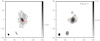 |
Fig. 1 Radio continuum images of the region around S 1 in ρ Oph. Left: at 1420 MHz with contours at 0.36, 0.52, 1.0, 2.0, 4.0, and 6.0 mJy beam−1. Right: at 610MHz with contours at 0.12, 0.3, 0.6, 2.0, 4.0, and 6.0 mJy beam−1. The beam sizes are shown in the bottom left corner of each panel. Asterisk marks the location of the embedded star S 1. The positional offsets (in arcseconds) are relative to the center α = 16h26m34. s175, δ = − 24° 23′ 28.′′3 (J2000). |
2.4 Auxiliary data
For comparison with our observations, we used maps of the J = 3–2 transition of CO, 13CO, and C18 O (White et al. 2015)and the J = 4–3 transition ofHCO+, all observed with the James Clerk Maxwell Telescope (JCMT) using the Heterodyne Array Receiver Program (HARP) receiver with a beam size of 14′′. The CO (and isotopologs) spectra were observed as part of the Gould Belt Survey and the HCO+(4–3) data set, corresponding to the proposal M11AU13, was downloaded directly from the JCMT archive at the Canadian Astronomical Data Centre(CADC). Both these data sets have also been presented and compared with the previous [C II] observations of the S 1 PDR by Mookerjea et al. (2018). The emission maps of the S(2) and S(3) pure rotational transitions of H2 observed with ISOCAM-CVF by Larsson & Liseau (2017) were also used for comparison.
3 Results
3.1 Properties of the ionized gas around S 1
The radio continuum emission from ionized plasma at 610 and 1420 MHz is shown in Fig. 1. The emission at 610 MHz shows a bright core surrounded by low brightness diffuse emission. The emission is extended up to 25′′, which corresponds to 0.02 pc at a distance of 137 pc. The emission at 1420 MHz extends up to 50′′. A central bright peak is observed surrounded by low surface brightness halo emission. The 610 and 1420 MHz images reveal an elongation in the northwest–southeast direction, which is more prominent in the 1420 MHz image. Such elongated structures in radio emission are often indicative of ionized jets from massive young stellar objects (YSOs; e.g., Purser et al. 2016). The total flux densities at these frequencies were obtained using a two-component Gaussian fit to the emission. The flux density of the central unresolved source is 5.6 ± 0.2 mJy, and that of the diffuse halo is 41.6 ± 3.0 mJy at 1420 MHz. The flux density of the central source at 610 MHz is 6.8 ± 2.0 mJy, and that of the diffuse emission is 47.6 ± 2.1 mJy.
Assuming that the diffuse emission at 1420 MHz is optically thin, we estimated the Lyman continuum photon rate and the spectral type of the star that causes the ionized emission. The Lyman continuum photon flux at 1420 MHz toward S 1 was estimated using the equation (Schmiedeke et al. 2016)
![\begin{equation*}\rm{\left[\frac{\textit{N}_{Ly}}{s^{-1}}\right]\,{=}\,4.771\,{\times}\,10^{42}\left[\frac{S_{\nu}}{Jy}\right]\left[\frac{\nu}{GHz}\right]^{0.1}\left[\frac{\textit{T}_e}{K}\right]^{-0.45}\left[\frac{d}{pc}\right]^2} ,\end{equation*}](/articles/aa/full_html/2021/04/aa40217-20/aa40217-20-eq1.png) (1)
(1)
where Sν is the flux density at frequency ν, which is 41.59 mJy at 1420 MHz, Te is the electron temperature, which is found to be 8200 K based on the electron temperature gradient across the Galactocentric distance (Quireza et al. 2006), and d is the distance to the source, which is 137 pc (Mookerjea et al. 2018). With Eq. (1), the Lyman continuum photon rate is found to be 6.7 × 1043 s−1. The estimated uncertainty in the electron temperature derived using the formulation by Quireza et al. (2006) is ≈ 100 K. Thus, no additional uncertainty in the estimated NLyc is introduced by this. If a single main-sequence star causes the ionization, then the spectral type of the Zero Age Main Sequence (ZAMS) star is earlier than B3V (Thompson 1984). For a B3V star with Teff = 18 700 K and R = 4.15R⊙, the Kuruczmodel (Castelli & Kurucz 2003) gives NLyc = 5.3 × 1043 s−1, and for a B2V star with Teff = 22 000 K and R = 5.19R⊙, we obtain NLyc = 8.2 × 1044 s−1. When the uncertainties of the derived NLyc are taken into account, we therefore conclude that star S 1 is most likely B2.5V or B3V, which is consistent with the Spectral Energy Distribution (SED) fitting by Mookerjea et al. (2018). Although the authors concluded a B4V type for the star, they noted that a B3V would fit equally well if a slightly higher extinction of 13.3 mag was adopted instead of 12.7 mag.
From the Very Large Array (VLA) high-frequency mapping of ρ Oph at 5 and 15 GHz, André et al. (1988) showed that the radio emission toward this region comes from a nonthermal unresolved source surrounded by a thermal extended halo. It is now known that S 1 is a close binary (Ortiz-León et al. 2017), the secondary of which causes the nonthermal emission. The flux density of the central source at 1420 MHz within the uncertainties is consistent with the flux measurements of André et al. (1988) and Stine et al. (1988). Using the flux densities of 6.8 and 5.6 mJy at 610 and 1420 MHz respectively, we derive a spectral index of − 0.2 ± 0.3, where the uncertainty in the derived index is contributed primarily by the uncertainty of the 610 MHz flux.
3.2 Morphology of the S 1 PDR cavity
InfraRed Array Camera (IRAC) and Multi-Band Imaging Photometer (MIPS) images (Padgett et al. 2008; Gutermuth et al. 2009) show that S 1 illuminates a large elongated spheroidal or egg-shaped cavity with a major axis at a position angle of 54° and a length of ~ 10.′5, and a minor axis of ~ 5′. The PDR emission toward the southwest (SW) is very strong, where it is blocked from expanding by the surrounding dense molecular cloud. Toward the northeast (NE), where the PDR shell emerges from the cloud, the emission is rather faint and barely visible. S 1 is ~ 80′′ from the SW tip of the PDR shell4. We used a combination of spatial and velocity information in the form of line-integrated emission, velocity–channel maps, and position–velocity diagrams along selected directions in the maps of the observed PDR tracers to understand the basic geometry of the PDR associated with S 1 (Fig. 2). To the west, the PDR borders the Rho Oph A ridge, which curves to the east south of the PDR. To the NW, the molecular cloud becomes very diffuse and is not detected in CO (White et al. 2015). In the past, no spectral line observations of the PDR emission east of S 1 have been reported, and most observations did not even fully capture the PDR emission to the N of S 1, which prompted Larsson & Liseau (2017) to model the PDR shell as a gaseous sphere with a radius of 80′′.
We mapped extended regions around S 1 in several PDR tracers: [C II], [O I] 63 and 145 μm, CO(6–5), and HCO+(4–3). Although HCO+(4–3) is not reallya PDR tracer and is mainly a dense gas tracer, it does show some excess emission from the PDR (Fig. 3). These data were compared with previous observations of the J = 3–2 transitions of CO, 13CO, and C18 O (Mookerjea et al. 2018). The emission seen in these PDR tracers matches the emission from neutral hydrogen (H I) and other PDR tracers such as 8 μm PAH emission and the S(2) pure rotational transition of H2 at 12.3 μm well (Fig. 3; see also Larsson & Liseau 2017). The visual extinction toward S 1 is ~ 13.3 mag and may even be higher over part of the nebula (Mookerjea et al. 2018). Additionally, the emission from all observed PDR tracers with the exception of [O I] 145 μm, which is optically thin, are heavily self-absorbed. The [13C II] F = 2–1 line is also optically thin, but relatively faint and only securely detected where the [C II] emission is strong. The [O I] 63 μm line is so strongly self-absorbed that no emission is seen in the υLSR range 3–4.5 km s−1 (Fig. 4). It therefore cannot be used as a tracer of the morphology of the PDR cavity. There is a strong CO(6–5) emission from the Rho Oph A ridge. However, near the SW tip of the PDR cavity, the emission from the PDR starts to dominate. The CO(6–5) and [O I] 145 μm maps also capturethe dense molecular PDR to the northeast of S 1.
The channel maps of [C II] and [O I] 145 μm (Fig. 4) show that the PDR emission is strongly redshifted on the southeastern side of the nebula, while the emission is primarily blueshifted on the northwestern side. The H I emission is also strongly redshifted on the southeastern side. This implies that gas is moving away from the observer on the southeastern side, while it is streaming toward the observer on the northwestern side, although blueshifted emission is also detected to the SE. At the SW tip of the PDR both blue- and redshifted gas is visible. The blueshifted emission dominates to the NW, and redshifted emission dominates to the SE. The same is true for the rest of the PDR nebula. Thisstreaming gas must be due to photoevaporation, which is commonly seen in PDRs. At the SE side of the cavity and toward the SW, the PDR emission is generally more redshifted than the emission from the surrounding cloud. Figure 5 shows that the CO(6–5) emission traces the NW PDR boundary extremely well at velocities from 1.5–3 km s−1 and the redshifted filament south of S 1. The CO(6–5) emission is strongly self-absorbed in the PDR in the velocity range 3–4 km s−1, similar to [O I] 63 μm, but not as extreme. The emission from the filament detected in CO(6–5) is by no means smooth. It shows two emission clumps in the velocity channels from 4.5 and 5.5 km s−1. The CO(6–5) emission is quite faint east of S 1, where the [O I]145 and [C II] emission is still quite strong. Faint CO(6–5) emission NE of S 1 is also visible, which may be unrelated to the PDR. The emission velocities of the H I 21 cm line agree in general with the velocities and features traced by the PDR gas, but less well with low-J CO emission. The H I emission is strongly affected by self-absorption between 3–6 km s−1 and shows the east–west extended filament, but only at higher velocities of 6.5–9 km s−1 than the PDR gas. This may be due to stronger self-absorption at lower velocities. Figure 6 shows three-color composites of [C II] and [O I]145 emission for different velocity ranges. This clearly shows that the emission at near-cloud velocities (coded green) is close to S 1, while the blueshifted emission arises from the northwest and the redshifted emission is to the southeast. The three-color plot of C+ additionally prominentlyshows a strong redshifted filament just SE of S 1.
In order obtain a more detailed view of the S 1 PDR cavity, we created Position–velocity diagrams (Figs. 7–10) of several PDR tracers along cuts parallel and perpendicular to the major axis of the cavity, as shown in Fig. 6. In the following, we refer to these position-velocity diagrams as pv-cuts. The [C II] map is more extended than the other maps, and [C II] still shows faint PDR emission 120′′ to the NE of S 1 (Fig. 7). There will be [C II] emission even further to the east, although it is likely to be faint. However, because the gas densities and FUV radiation field is low, it is possible that only the rim outlining the PDR shell can be detected. The position–velocity diagrams show that the SW tip of the PDR is somewhat redshifted, suggesting that the PDR is tilted away from us in the SW and approaches us in the NE. The perpendicular pv-cuts across the PDR cavity show that the cavity is less extended to the SE (~ 80′′) than to the NW (~ 100′′), suggesting that the surrounding molecular cloud must be much denser at the SE side than at the NW side, which slows down the expansion of PDR cavity to the SE compared to the NW side. The perpendicular pv-cuts also show strong blueshifted emission to the NW with more red- than blueshifted emission to the SE. The flip from red- to blueshifted emission occurs roughly at the symmetry axis of the PDR cavity. The HCO+ emission, which is dominated by the surrounding cloud, also shows the same velocity gradient across the PDR cavity. These pv-cuts suggest thatat the SE side of the cavity, the surrounding cloud must be very dense at the front side, that is, the side facing us, while at the NW side, the cloud is denser on the back side. This forces the photo-evaporation flow from the PDR to be mostly redshifted in the SE and blueshifted in the NW. We visualize this in the cross-sectional view of the PDR SW of S 1 (Fig. 2), which is a very simplified picture because the PDR layer is by no means smooth. There may be ridges and valleys, and there can also be dense clumps of gas inside the PDR, similar to what appeared to be the case for NGC2023 (Sandell et al. 2015). There is a strong redshifted filament just SE of S 1, which stands out prominently in the [O I] 63 μm channel maps at velocities from 5–6.5 km s−1 (Fig. 4). This filament is also seen in the [O I] 145 μm, [C II], H I, and CO(6–5) channel maps (Fig. 4 and 5).
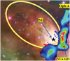 |
Fig. 2 Composite-color image of the S 1 PDR derived using the 3.6, 4.5, and 8 μm Spitzer observations (Padgett et al. 2008). Also shown is a cartoon of the morphology of the PDR that is derived in this paper on the basis of the spatial and velocity dependence of emissions in multiple tracers. The red and blue surfaces show the red- and blueshifted fronts of the PDR. The color map corresponds to N2 H+ emission (Larsson & Liseau 2017) from the molecular cloud to the west. The yellow line demarcates the boundary of the PDR as identified from our [C II] observations and the 8 μm emission. |
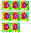 |
Fig. 3 Comparison of the 8 μm continuum image observed with IRAC/Spitzer (color) with contours of integrated intensity images of tracers (marked) overlaid on the 8 μm continuum image observed with IRAC/Spitzer. The color scale is shown in the wedge to the right of the top row, with numbers in units of MJy/sr. For each of the tracers shown as contours, levels are shown at the top of the panel and beams are shown in the top left corner of each panel. The range of velocities over which integrations were made are as follows: [C II] −0.5 to 7.5 km s−1, [O I] 145 μm 1 to 5.5 km s−1, [O I] 63 μm 0.5 to 6.5 km s−1, H I −0.5 to 5 km s−1, CO(6–5) 0 to 10 km s−1, HCO+ (4–3) 0 to 10 km s−1, and [13 C II] F = 2–1 1 to 5 km s−1. The positional offsets are relative to the center α = 16h26m34. s175, δ = − 24° 23′ 28.′′3 (J2000). The asterisk and the triangle mark the positions of S 1 and VLA 1623, respectively. The numbers in the top left panel mark selected positions that are studied in detail. The offsets for the positions in arc seconds are 1(−61,45), 2(−33,6), 3(−31,−31), 4(32,−23), and 5(60,−45). |
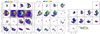 |
Fig. 4 Channel maps of [C II] (left), [O I] 63 μm (middle), and [O I] 145μm (right). The color scale for each map is shown next to the map. Velocities corresponding to the channel are marked in each panel. The red star marks the position of S 1. The positional offsets (in arcseconds) are relative to the center α = 16h26m34. s175, δ = − 24° 23′ 28.′′3 (J2000). The area mapped in CO(6–5) is shown with dashed boundaries in the top left panel of the [C II] channel map. |
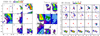 |
Fig. 5 Same as in Fig. 4, but for channel maps of CO(6–5) (left), 13 CO(6–5) (middle), and H I (right) emission. The area mapped in CO(6–5) is smaller than that of the maps in Fig. 4. The area mapped in 13CO(6–5) is marked with dashed boundaries in the top left panel of the CO(6–5) channel map. |
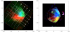 |
Fig. 6 Three-color composite images showing the [C II] and [O I] 145 μm emission in different velocity channels. The orthogonal sets of lines show the cuts along which the position-velocity diagrams are derived. Left: [C II] emission in velocity interval υLSR = −0.5–1, 1.5–3, and 4.5–7 km s−1 shown as blue, green, and red channels, respectively. The contours show the [C II] emission in the velocity interval −0.5–7 km s−1. Right: [O I] 145 μm emission in the velocity intervals υLSR = 1–2.5, 3–4, and 4–5.5 km s−1 as blue, green, and red channels, respectively. The contours show the [O I] 145 μm emission in the velocity interval 1–5.5 km s−1. |
 |
Fig. 7 Position–velocity diagrams of [C II] emission along the parallel (top) and perpendicular (bottom) cuts shown in Fig. 6. The angular resolution is 18′′. The two red vertical lines mark the vlsr = +3.5 km s−1 for [C II] and the [13C II] F = 2–1 hyperfine line, which is offset by +11.2 km s−1 in the rest frame of [C II], or +14.7 km s−1. The contour levels are plotted with a linear step size and enhanced with a gray scale from 1 K to 1.25 times the peak temperature. For the parallel cuts, 10 contours from 1 to 73 K with the peak temperature at 73.1 K are shown. The contour levels for the perpendicular pv-plots are ten linear contours from 1 to 76 K and gray scale from 1 to 96 K. Offsets are relative to S 1, which is at 0′′. The parallelcuts extend from the NE to the SW starting from the south. The perpendicular cuts extend from the NW to the SE and start east of S 1. |
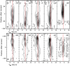 |
Fig. 8 Position–velocity diagrams of [O I] 145 μm emission along the same parallel (top) and perpendicular (bottom) cuts as [C II] in Fig. 7. The angular resolution is the same as for [C II], i.e., 18′′. Eight linear contours extending from 1.25 to 42 K are shown, while the gray scale is between 1.25 and 52.9 K. |
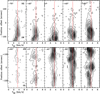 |
Fig. 9 Position–velocity diagrams of HCO+(4–3) emission along parallel (top) and perpendicular (bottom) cuts shown in Fig. 6 and plotted in the same way as Figs. 7 and 8 using the same angular resolution as for [C II]. Ten linear contours from 0.3 to 6.9 K are shown, and the peak intensity is 7.0 K. To the NE, the HCO+ is barely detectable 60′′ from S 1, confirming that the density of the surrounding cloud falls off toward the NE. The southwestern most perpendicular position velocity cut 120′′ west of S 1 does not cross the PDR, but is plotted to illustrate that the emission in the Rho Oph A ridge is more blueshifted than the emission from the S 1 PDR. |
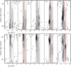 |
Fig. 10 Position–velocity diagrams of CO(6–5) emission along parallel (top) and perpendicular (bottom) cuts shown in Fig. 6 and plotted in the same way as Figs. 7 and 8using thesame angular resolution as for [C II]. Ten linear contours from 0.8 to 68 K are shown, and the gray scale extends from 0.8 to 85 K. In the parallel cuts, red- and blueshifted emission from the VLA 1623 outflow in the SW is observed. The blueshifted outflow lobe in the SE is detected in the perpendicular cut 80′′ from S 1. This bipolar outflow is unrelated to the S 1 PDR. There is no evidence for PDR emission in the perpendicular cut 80′′ NE of S 1. The CO(6–5) emission is faint and most likely comes from the surrounding molecular cloud. |
3.3 Analysis of spectral profiles
The [C II], CO(6–5), and H I spectra throughout the observed map show self-absorption, along with red- and blueshifted line
wings. The [C II] lines are the broadest of the PDR and molecular tracers. The [O I] 145 μm spectra typically show a single peak centered on the absorption in the [C II] spectra, as well as an extended blue wing at a few positions. The [O I] 63 μm, on the other hand, is completely absorbed between 3–4.5 km s−1. The spectra of 13CO(6–5) show absorption dips at positions close to the CO(6–5) peak, but the emission is single-peaked at positions to the southwest of the map as well as in the region immediately to the west of the S 1. This suggests that the foreground material is optically thin in [O I] 145 μm throughout the entire map, while 13CO(6–5) is still moderately optically thick in a few places. Figure 11 shows the spectra at the location of S 1 and five additionally selected positions (shown in Fig. 3) within the mapped region, which sample a variety of [C II] line shapes that are representative of the entire map.
Our observations are deep enough to detect the F = 2–1 transitions of [13C II] at 90 positions in the entire region. Closer inspection of the [C II] spectra at five out of the six selected positions also reveal clear detection of the F = 2–1 transition of [13C II]. Unlike the [C II] profiles, which show a strong absorption dip, the [13 C II] spectra peak exactly at the location of the [C II] dip (Fig. 12). Similar trends are also visible when the [O I] 63 and 145 μm spectra are compared at these five positions (Fig. 13).
We start by trying to understand the role of the foreground material in shaping the [C II] and [O I] 63 μm spectral profiles characterized by deep self-absorption. We modeled the observed [C II] and [O I] 63 μm spectra considering two layers, a background layer (the main PDR) that emits, and a foreground cloud that absorbs. We took an empirical approach and assumed that the [13C II] and [O I] 145 μm spectra, which are optically thin, represent (except for a scaling factor) the [C II] and the [O I] 63 μm spectra, respectively,that the PDR would emit in the absence of the foreground absorbing gas. The scaling factor used for the [13 C II] spectrum is 12C/13C = 70 (after correcting for the detection of only the strongest of the hyperfine structure line of [13 C II], which accounts for 0.625 of the total [13C II] intensity). The ratio of the [O I]63/[O I]145 intensities in the background-emitting gas depends strongly on the physical conditions. We used a scaling factor of 2 for the [O I] 145 μm spectrum, which corresponds to F63 μm/F145 μm of 24, a value that is representative for warm, medium dense PDR conditions (Goldsmith 2019, e.g., Fig. 5). Thus, we consider that at each position the [C II] ([O I] 63 μm) spectrum is given by the scaled [13 C II] ([O I] 145 μm) spectrum and the foreground gas is a pure absorbing screen with a constant velocity, width, and optical depth. In this approach, we assume that the effect of the foreground material on the background emission is to attenuate the latter by the factor ![$\exp\left({-\tau_0\exp[-4\ln 2\,(\upsilon-\upsilon_0)^2/\Delta \upsilon^2]}\right)$](/articles/aa/full_html/2021/04/aa40217-20/aa40217-20-eq2.png) . Here τ0, υ0, and Δυ denote the peak optical depth, the velocity at which the foreground cloud has a value of τ0, and the full width at half maximum (FWHM) of the foreground absorption profile. In order to generate the [13 C II] spectra with higher fidelity, we coadded the [13C II] and all other spectra over 20′′ with centers at the selected offsets. Additionally, to improve the quality of the template spectra generated from [13 C II] and [O I] 145 μm, we did not use the observed spectra to simulate the emission, but instead we used the Gaussian profiles generated from fits to the observed spectra. Figures 12 and 13 also show the results of this two-slab modeling at five selected positions in the observed region.
. Here τ0, υ0, and Δυ denote the peak optical depth, the velocity at which the foreground cloud has a value of τ0, and the full width at half maximum (FWHM) of the foreground absorption profile. In order to generate the [13 C II] spectra with higher fidelity, we coadded the [13C II] and all other spectra over 20′′ with centers at the selected offsets. Additionally, to improve the quality of the template spectra generated from [13 C II] and [O I] 145 μm, we did not use the observed spectra to simulate the emission, but instead we used the Gaussian profiles generated from fits to the observed spectra. Figures 12 and 13 also show the results of this two-slab modeling at five selected positions in the observed region.
Table 2 presents the results of fitting of the two-component model to the [C II] and [O I] 63 μm spectra. The C+ absorbing layer shows peak opacities (τ0) between 3.5–4.8 at velocities (υ0) between ~ 3.5–4.4 km s−1, with a width (Δυ) between 1.4–3.4 km s−1. The O0 absorbing layer gives rise to peak opacities for [O I] 63 μm of 4–8 at velocities between 3.7–4.1 km s−1 with a line width of 1.7–2.2 km s−1.
We point out that in particular the blue part of the [C II] spectrum is not fully reproduced at some of the positions, probably because the [13 C II] lines are fainter and do not trace the line wings where [C II] is optically thin. Similarly, at (32,−23) for the fit to the [O I] 63 μm spectrum, a broader redshifted velocity component is completely missing, and part of the blue wing is not fully reproduced by the fit based on the [O I] 145 μm spectra. For (−31,−31) and (−61,45), the fits are somewhat lacking at lower velocities. The central velocity and line width of the foreground absorbing component derived for fits to the [C II] and [O I] 63 μm spectra are consistent with the two-component LTE-based modeling that was performed by Mookerjea et al. (2018). However, the fit presented here is better constrained because of the availability of [13 C II] and [O I] 145 μm.
Table 2 presents the column densities in the lower energy level of C+ and O0 in the foreground absorbing gas estimated based on the ∫ τ dυ values derived from the fits and using the relation
 (2)
(2)
where gl and gu denote the statistical weights of the lower and upper energy levels, Aul denotes the Einstein A-coefficient for spontaneous emission, and λ denotes the transition wavelength.
We obtain that N(O) of the absorbing gas is between (2.3–3.0) 1018 cm−2. For these column densities, based on non-LTE calculations using RADEX (van der Tak et al. 2007), the [O I] 145 μm line is optically thin over a large range of temperatures (20–300 K) and volume densities (104 –107 cm−3). This is also consistent with our observations. Because the TA ratio for the two [O I] lines depends on the physical conditions, there is significant uncertainty in the derived values of the peak optical depth, although the fitted central velocity and line width are fairly robust against the assumed scale factor. Furthermore, the estimate of N(O0) assumes that all O atoms in the absorbing layer are in the ground 3P2 level, which is reasonable because [O I] 145 μm is not seen inabsorption. We estimate the column density of C+ in the absorbing gas to be between (1–2) × 1018 cm−2. We note that the estimate of N(C+) assumes that more than 95% of the C+ are in the ground state. For excitation temperatures of foreground gas higher than 25 K, the derived N(C+) is a lower limit. Thus the N(O0)/N(C+) ratio in the foreground absorbing layer is between 2–3.
This toy model confirms that both the [C II] and [O I] 63 μm spectra are strongly self-absorbed by the foreground PDR gas. Additionally, based on the derived velocity at which the peak optical depth occurs for both species (>3.2 km s−1), we also find that the absorption occurs due to the temperature gradient in the PDR gas itself and not due to the ambient molecular gas that is traced by the J = 3–2 transitions of CO and its isotopologs.
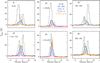 |
Fig. 11 Comparison of spectra of [C II], [O I], C18O(3–2), CO(6–5), and 13CO(6–5) transitions at the selected positions. The positions are shown in Fig. 3. The data set corresponding to the C18 O(3–2) spectra shown here was presented by Mookerjea et al. (2018). All spectra have been coadded across a 20′′ field. |
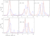 |
Fig. 12 Comparison of [C II] (red) and [13C II] (blue) spectra averaged over 20′′ with centers at offsets shown in the panels. The [13C II] spectra have been scaled by a factor of 20 to make the spectra visible alongside [C II]. The smooth curve (black) shows the fit to [C II] spectrum obtained by attenuating the abundance factor scaled [13 C II] spectrum by the absorption due to the foreground cloud. |
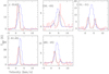 |
Fig. 13 Comparison of [O I] 63 (red) and [O I] 145 μm (blue) spectra coadded over 14′′ with centers at offsets shown in the panels. The smooth curve (black) shows the fit to the [O I] 63 spectrum obtained by attenuating the scaled (by a factor 2 corresponding to the typical ratio between the two [O I] lines in temperature units) [O I] 145 μm spectrum by absorption due to foreground material. |
Peak optical depth, corresponding velocity, and the FWHM of the foreground absorbing gas derived from modeling the [C II] and [O I] 63 μm spectra with a two-slab model.
3.4 Temperature of the [C II] emitting PDR gas
In our analysis of the absorption features in the [C II] profile, we have considered the background [C II] profile to be an optically thin scaled-up version of the [13C II] profile. However, based on the recent [C II] observations of most of the Galactic PDRs it is likely that the background PDR emission probably has an optical depth close to 1. Guevara et al. (2020) performed an elaborate fitting procedure involving multicomponent LTE components to explain optically thick background [C II] spectra that are absorbed by a foreground layer of gas. Here we approximated the background [C II] spectrum by assuming it to be a scaled-up version of the [13 C II] spectrum modulated by an optical depth of 1. The Planck-corrected peak of the optically thick [C II] spectrum so derived provides a lower limit of the temperature of the [C II] emitting PDR gas. Table 2 also presents the temperatures of the [C II] emitting PDR gas at the selected positions estimated using this method.
We used the integrated line intensities of the optically thin [13 C II] spectra at these selected positions to estimate N(C+). We estimated the total integrated intensity of [13C II] by considering that the observed F = 2–1 transition accounts for 62.5% of the total intensity (Table 3). The column density of 13C+ was estimated following Eq. (26) from Goldsmith et al. (2012),
![\begin{equation*}N(^{13}{\textrm{C}^+})\,{=}\, {\frac{8\pi {\textrm{k}}_{\textrm{B}}\nu_{\textrm{ul}}^2}{\textrm{A}_{\textrm{ul}}\textrm{hc}^3} \left[1+0.5{\textrm{e}^{91.25/{T}_{\textrm{kin}}}}\left(1+\frac{\textrm{A}_{\textrm{ul}}}{\textrm{C}_{\textrm{ul}}}\right)\right] \int {\textrm{T}}_{\textrm{mb}}\textrm{d}\upsilon},\end{equation*}](/articles/aa/full_html/2021/04/aa40217-20/aa40217-20-eq4.png) (3)
(3)
where νul = 1900.4661 GHz, Aul = 2.3 × 10⁻⁶ s−1, Tkin is the gas kinetic temperature, the collision rate is Cul = Ruln with Rul being the collision rate coefficient with H2 or H0, which depends on Tkin, and n is the volume density of H. For nH > 104 cm−3, Cul ≫ Aul so that the last term in Eq. (3) can be neglected.
We assumed a 12C/13C ratio of 70 based on the galactocentric distance of the S 1 PDR (Wilson & Rood 1994). Using the observed integrated [13 C II] intensities and the estimated Tkin (Table 2), we estimate that N(C+) at the selected positions is between 1.3–3.8 × 1018 cm−2 (Table 3). Comparing the total C+ column density derived here with N(C+) estimated for the foreground absorbing gas (Table 2), we find that for all positions the column density of the colder foreground gas is approximately one-third of the N(C+) of the background PDR gas.
Results of fitting Gaussian profiles with single velocity components to observed spectra at selected positions.
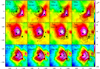 |
Fig. 14 Comparison of distribution of [C II], [O I] 145 μm, CO(6–5), and HCO+ (4–3) emission and the column density, dust temperature, and FUV intensities estimated from PACS continuum data observed as part of Herschel Gould Belt Survey. The color scales are shown at the far right of each row of panels. The contour levels for [C II], [O I] 145 μm, and HCO+ (4–3) are at 20–100% (in steps of 10%) of the peak values of 191, 88, and 14 Kkm s−1 respectively. For CO(6–5)the contours are at 40–100% of the peak of 136 km s−1. Circles correspond to radii of 45′′ and 75′′. |
4 PDR of S 1
Figure 14 shows a comparison of the observed distribution of the PDR and high-density tracers with the molecular hydrogen column density, dust temperature, and FUV intensity, all derived from the dust continuum detected with PACS as part of the Herschel key program in the Gould Belt Survey (André et al. 2010). The column density and dust temperature maps are directly taken from the Gould Belt Survey website, and we estimated the FUV intensity from the observed FIR intensity as described in Mookerjea et al. (2018). The circles drawn in Fig. 14 are centered on S 1 with radii of 45 and 75′′ to guide the eye. The column density peak in the Oph A cloud is close to the position of VLA 1623. The dust temperature peaks at a position slightly offset from S 1 and closer to the [C II] peak and the embedded YSO LFAM 9. The peak in the FIR continuum map is located close to S 1 and also to the southwest (Fig. A.1. in Mookerjea et al. 2018). As indicated earlier, the PDR is bound by the dense ambient cloud to the southwest and is more tenuous to the northeast. The fraction of stellar FUV radiation that is intercepted by the cloud is therefore likely to be larger toward the southwest than at positions toward the east and northeast, which are radially equidistant from S 1. The [C II] traces the entire PDR gas, which is also seen in the FUV map derived from the FIR continuum maps. The [O I] 145 μm, which has a higher critical density, preferentially picks up the denser and warmer edge-on PDR rim to the west.The CO(6–5) traces only the PDR clumps within a very narrow strip, and the HCO+ (4–3) traces the higher density (and column density) molecular clouds in the Oph A ridge, which also harbors the YSO VLA 1623.
Table 3 presents results of fitting Gaussian profiles to the optically thin spectra of [13 C II], [O I] 145 μm, C18 O (3–2), and 13CO(6–5) at the positions already analyzed in Fig. 12. We find that the [13 C II] and [O I]145 lines are significantly broader than the 13CO(6–5) lines, except at the position (−61,45), which corresponds to the peak of [O I] 145 μm as well as 13CO(6–5). Additionally, the central velocities of the PDR tracers are red- and blueshifted relative to the molecular cloud tracer, depending on whether the positions are to the north or south of S 1, respectively. The C18 O(3–2) primarily traces the ambient molecular cloud and hence typically peaks around 3.1 km s−1.
4.1 FUV field
The distribution and emission from the PDR is primarily a function of the FUV (6 eV ≤ hν < 13.6 eV) radiation field and volume density of the PDR gas. Star S 1 is the primary source of FUV radiation for this PDR. Based on the observed radio continuum flux at 1420 MHz, we estimate that S 1 has a spectral type of B2.5–B3V. We thus used the Schmidt–Kaler relation for a B3V star (Teff = 18 700 K and a radius of 4.15 R⊙) and a Kurucz model atmosphere to estimate the FUV radiation field distribution considering only projected distances and geometrical dilution. The FUV field is typically expressed in units of the Habing (1968) value for the average solar neighborhood FUV flux, 1.6 × 10⁻³ ergs cm−2 s−1. We find that at a radial distances of 45′′ and 75′′ from S 1, the unattenuated FUV field from S 1 is 2.70 × 10⁴ and 8500 G0, respectively. An alternative method of estimating the strength of the FUV radiation in the region involves the use of the observed total far-infrared (FIR) intensity, assuming that the entire FUV energy is intercepted and absorbed by the grains and is reradiated in the FIR. We used the far-infrared observations of Herschel/PACS to estimate the values of FUV radiation field around S 1 (Fig. 14). We find that the observed FIR distribution is neither spherically symmetric around S 1, nor does it peak at the position of S 1. The peak in FIR emission (coinciding with the peak Tdust) is primarilyto the north-west, where the derived FUV radiation is around 4000 G0 at a radius of 75′′. To the eastat similar radii from S 1 the estimated FUV emission is ~ 1200 G0. By making a pixel to pixel comparison, we find that only for the ridge-like structure to the north–west the FUV flux predicted from the S 1 FUV radiation and from the FIR continuum agree to within a factor of 2. For regions between 40′′ to 75′′ from S 1 and at the ridge in the west, the two estimates differ by up to a factor of 10. The discrepancy between the FUV radiation field derived theoretically considering only geometric dilution and the field derived indirectly from the observed far-infrared radiation can be due to (a) the emission in the far-infrared continuum that arises from regions thatare at much larger distances than the projected distance used here, (b) FUV radiation escaping the region without being intercepted by material, particularly to the east and northeast, and (c) presence of very high AV clumps, which attenuate the FUV drastically but are too small to be detected in single-beam continuum observations.
As discussed in Sect. 3.1, the region is bound in the west and southwest by the dense Rho Oph A ridge and possibly freely expands to the northeast. The structures visible in the far-infrared continuum images primarily trace the column density of dust (and gas) along the lines of sight, as is shown in the H2 column density maps generated from the same PACS maps (Fig. 14). The lower levels of FIR continuum emission closer to S 1 as well as to the east is therefore a result of lower column densities of dust (and molecular gas) in these regions, while the higher FIR continuum emission to the northwest indicates the presence of higher column density clumps, which is also substantiated by the detection of HCO+ (4–3) with the JCMT and NH3 with the Green Bank Telescope (Friesen et al. 2017).
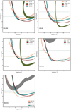 |
Fig. 15 Comparison of observations with the prediction of line intensities as a function of nH and G0 from an updated version of the Kaufman et al. (2006) PDR models (Wolfire, priv. comm.). For all positions except for (32,−23) and (60,−45), the [13 C II] intensities are beyond the values predicted by the models. The horizontal dashed lines correspond to the values of G0 estimated from the FIR intensities (lower) and from the stellar FUV radiation scaled only by geometrical dilution due to the increase in distance from S 1. |
4.2 Comparison of observed intensities with PDR models
We compared the observed intensities of optically thin tracers [13 C II], [O I] 145 μm, and 13CO(6–5) with the predictions of plane–parallel steady-state PDR models, which self-consistently calculate the intensities as a function of the FUV flux and gas density of H nuclei nH. These PDR models are from an updated version of the models by Kaufman et al. (2006) (Wolfire, priv. comm.). We performed the analysis at the five selected positions because they lie at different radial distances from S 1 to the east–west and north–south of S 1, thus tracing the distribution of the spectral lines arising from the PDR reasonably well. The S(2) and S(3) transitions of H2 are produced byFUV pumping, and hence the intensities are proportional to the FUV radiation. At the positions at which the rotational lines of H2 S(2) and S(3) have been detected, we also compared their intensities with the PDR model predictions. Figure 15 shows a comparison of the observed intensities of the tracers (shown as contours) with the values predicted by the models. The lower and upper limits of the FUV intensities (shown by dashed horizontal lines in Fig. 15) are determined by the values derived from the FIR intensities and from the stellar FUV radiation field, respectively (Sect. 4.1). At most positions, the observed [13 C II] exceeds the intensities predicted by the models for the entire parameter space explored, hence the corresponding contours are not visible in Fig. 15.
The critical densities (and Eu) for [13C II], [O I] 145 μm, and CO(6–5) are 3000 cm−3 (91 K), 5.8 × 106 cm−3 (325 K), and 2.9 × 105 cm−3 (116 K), respectively. The S(2) and S(3) transitions of H2 have critical densities (and Eu) of 2.2 × 105 cm−3 (1682 K) and 9.4 × 105 cm−3 (2504 K), respectively. Thus [O I]145, 13CO(6–5) and S(2) H2 transitions could arise from PDR gas of similarly high densities, while [13 C II] traces the low-density PDR. Although the H2 lines have rather high critical densities and high upper energy levels, these are produced by FUV pumping. For values of G0 ∕n < 10−2 the intensities of the S(2) and S(3) lines of H2 depend on the FUV intensities, while for G0∕n > 10−2, the same intensities are indicators of the densities (Kaufman et al. 2006). At the selected positions, the FUV radiation field lies between 103 –104.5, which implies that G0∕n = 10−2 corresponds to n = 105–106.5 cm−3. For most positions, the [O I]145 and H2 line intensities indicate n ~ 104 cm−3, while 13CO(6–5), where detected, suggests n > 105 cm−3. For most positions, the observed [13C II] intensities exceed the intensities predicted by the model, which correspond to the densities indicated by the [O I]145 and the estimated range of FUV radiation fields, by factors of 1.2–3. The largest discrepancy, a factor of 3–6, is seen at the position (−33,6). Additionally, the model predictions for the [O I]145/[13C II] intensity ratios indicate unrealistically high (for [13C II] emission) densities at all positions, which is not corroborated by high-density tracers such as CO(6–5) and HCO+(4–3).
Comparison of the observed emission from the S 1 PDR with models clearly shows the contributions of gas at primarily three different density regimes, 105 –106 cm−3, 103.5–104.5 cm−3, and < 103.5 cm−3, although the [13C II] emission is significantly underproduced by the models, as is seen both from the [13 C II] intensity and the [O I]145/[13C II] intensity ratio. The highest density regions are traced by 13CO(6–5) and to some extent by [O I] 145 μm. Additionally, [O I] 145 μm emission is excited in the medium-density gas as well, which is also traced by the H2 S(2) and S(3) lines. The most diffuse component is primarily traced by the [13 C II], and for positions (−33,6) and (−61,45), the observed intensities, estimated to stem only from the diffuse component, still far exceed the values predicted by the PDR models.
The lower [13C II] intensities and correspondingly high [O I]145/[C II] ratio predicted by the face-on uniform density plane-parallel PDR models cannot be explained either by stacking layers of these PDRs along the line of sight or by changingthe viewing angle of the model. The most plausible explanation for higher observed [13 C II] intensities relative to [O I]145 line is in terms of the higher filling factor of the [13 C II] emission, which typically should have significant contribution from the diffuse gas than from the high-density gas emitting mostly in [O I]145. Such discrepancies are also expected to arise from the shadowing effects of clumps as well as from the penetrability of nonuniform density PDRs consisting of clump and interclump gas (Stutzki et al. 1988). Use of three-dimensional PDR models with inhomogeneity is needed, but these models also involve additional parameters that need to be predetermined using other observational constraints. In the case of the S 1 PDR, the self-absorption of the main PDR tracers and the complex geometry of the region does not allow us to further observationally constrain the parameters for these clumpy PDR models. Qualitatively, we can conclude that the fraction of [13 C II] intensity putatively arising from diffuse PDR gas that is higher toward the west of S 1 is likely to be an indicator of increased clumpiness toward the west.
5 Discussion and conclusion
The multiple emission and absorption components along the line of sight toward the PDR associated with the S 1 star in the ρ Ophiuchus molecular cloud results in complicated spectra that are difficult to interpret. In this region, the emission arising from the PDR and the molecular cloud overlap, most spectra are self-absorbed, and additional foreground filaments criss-cross the region. The S 1 PDR is restricted by the dense Oph A molecular cloud to the west and southwest and appears to be expanding freely to the east. The PDR is tilted and somewhat warped, with the front surface (facing the observer) of the southeastern side of the cavity being very dense, and on the NW side, the cloud is denser at the far side. The gas distribution in the PDR is rather inhomogeneous, with clumps and ridges arising due to the disruption of the dense ambient molecular cloud by the radiation from star S 1 and also by the embedded YSOs. Analysis of the emission from the photon-dominated gas suggests at least three density components consisting of high-density (106 cm−3) clumps and medium-density (104 cm−3) and diffuse (103 cm−3) interclump medium.
Using the velocity information and the optically thin spectra of [13 C II] and [O I] 145 μm, we have shown that the absorption features in [C II] and [O I] 63 μm arise due to the foreground layers of the same PDR. The ratio of column densities of C+ and O0 in the diffuse foreground PDR layers, within the limits of uncertainties introduced particularly by the assumed value of the scaling factor for the [O I] lines is between 2–3, which is comparable to the solar [O]/[C] abundance ratio of 3.5. Spectral analysis of our data allowed us to qualitatively constrain the temperature of the absorbing layers. The presence of heavy foreground absorption in the [O I]63 spectra and the complete absence of self-absorption in the [O I]145 line profiles suggest a low-excitation status of the foreground gas, lower than the energy of the OI 3P1 level, which is 227 K above ground. On the other hand, the prominent self-absorption in the CO(6–5) line indicates a somewhat elevated temperature of the absorbing gas, sufficient to populate the J = 5 level (80 K above ground).
The [C II] spectra show the self-absorption dips even far to the east, and the rarer isotope 13C+ has been detected at a large number of positions, suggesting an N(C+)~ of a few times 1018 cm−2 over an extended region. The estimated N(C+) lies within the typical range of values between 1018 –1019 cm−2 that is found in Galactic PDRs (Ossenkopf et al. 2013; Mookerjea et al. 2019). The H2 column density estimated from dust continuum emission maps ranges between 1–2.5 × 1022 cm−2 at these positions. This suggests values of [C+ /H2] ranging between (1.5–4.8) × 10−4, which leads to C+ /H = (0.8–2.4) × 10−4. The derived value of C+/H is consistent with the value C+ /H = 1.5 × 10⁻⁴ obtained considering solar abundance with the assumption that half of the carbon is in C+. The uncertainties in the value of N(C+) arise due to the assumed values of Tkin used, which were derived from the peak of the Planck-corrected [C II] spectra (Sect. 3.4) and are likely a lower limit to the temperature.
Based on the comparison of the observed intensities with the PDR models (Fig. 15), we have identified the range of densities that might explain the [O I] 145 μm intensities. We find that for the [O I] 145 μm peak, densities between 104 –105 cm−3 can explain the [O I]145 intensities. When non-LTE approximations are used, the observed intensities for these densities can only be explained by Tkin > 100 K (consistent with our derived  of 157 K) and for N(O0) between (1.5–3) × 1019 cm−2. Similar considerations suggest that for positions (−33,6) and (−31,-31), the observed intensities can be explained by a Tkin of 100 K and N(O) of (2–3) × 1019 cm−2 for n = 105 cm−3. For these two positions the lower-density-higher-G0 solution requires Tkin = 120 K and N(O) = 5 × 1019 cm−2. However, we emphasize that it is likely that the high- and low-density gas with possibly different filling factors both contribute to the emission. For positions to the west of S 1, as pointed out earlier, the FUV flux derived from FIR intensities is lower than the value expected from the estimated stellar radiation because part of the radiation is not intercepted by dust. For these positions, the higher FUV radiation values corresponding to the geometrically diluted stellar radiation are likely to be a closer representation of reality. The densities at these positions are thus ~ 104 cm−3, which corresponds to N(O) ~ 1019 cm−2 for Tkin = 100 K. Most of the observed [O I] 145 μm intensities can be explained by N(O) between (1–3) × 1019 cm−2. On the other hand, the column density N(O) of the self-absorbing gas dominating the [O I] 63 μm profile is only one-tenth of the O0 column density, which shows up in emission. The total N(O) estimated for the S 1 PDR is similar to the column densities (> 1019 cm−2) seen in dense molecular gas in sources such as OMC-1 (Herrmann et al. 1997) and L1689N (Caux et al. 1999). Typical values of N(O) estimated from observations lie between 1018 –1019 cm−2 (Vastel et al. 2000, 2002).
We estimate the gas pressure to be in the range of 104 – 108 K cm−3 for densities between 103.5– 106 cm−3 and temperatures, Tkin, of 60–120 Kin the three gas components we identified. The ambient high-density cloud that harbors the ρ Oph A region tothe west with typical temperature of 10–20 K and a density of 106 cm−3 (Liseau et al. 2015) has a thermal pressure of around 107 cm−3. Although we have detected photoevaporation flows, no streaming motions indicative of a large pressure gradient were observed in the PDR and to the west, where it touches the high-density molecular cloud. Interestingly, for an assumed temperature of Tkin of 100 K, the density of the PDR gas that primarily contributes to the thermal pressure and maintains equilibrium at the interface with the molecular gas would be 105 cm−3. This is consistent with the medium-density interclump medium as identified from our analysis of the emission from the PDR gas.
Acknowledgements
The authors would like to thank W. Vacca for his help regarding the stellar type of S 1 and M. Wolfire for allowing the use of the updated PDR models prior to publication. BM acknowledges the support of the Department of Atomic Energy, Government of India, under Project Identification No. RTI 4002. Based on observations made with the NASA/DLR Stratospheric Observatory for Infrared Astronomy (SOFIA). SOFIA is jointly operated by the Universities Space Research Association, Inc. (USRA), under NASA contract NAS2-97 001, and the Deutsches SOFIA Institut (DSI) under DLR contract 50 OK 0901 to the University of Stuttgart. The development of GREAT was financed by the participating institutes, by the Federal Ministry of Economics and Technology via the German Space Agency (DLR) under Grants 50 OK 1102, 50 OK 1103 and 50 OK 1104 and within the Collaborative Research Centre 956, sub-projects D2 and D3, funded by the Deutsche Forschungsgemeinschaft (DFG). This research has made use of the VizieR catalog access tool, CDS, Strasbourg, France. The original description of the VizieR service was published in A&AS 143, 23. This research has made use of data from the Herschel Gould Belt survey (HGBS) project (http://gouldbelt-Herschel.cea.fr). The HGBS is a Herschel Key Programme jointly carried out by SPIRE Specialist Astronomy Group 3 (SAG 3), scientists of several institutes in the PACS Consortium (CEA Saclay, INAF-IFSI Rome and INAF-Arcetri, KU Leuven, MPIA Heidelberg), and scientists of the Herschel Science Center (HSC).
References
- Andre, P., Montmerle, T., Feigelson, E. D., et al. 1988, ApJ, 335, 940 [Google Scholar]
- André, P., Men’shchikov, A., Bontemps, S., et al. 2010, A&A, 518, A102 [Google Scholar]
- Belitsky, V., Lapkin, I., Fredrixon, M., et al. 2018, A&A, 612, A23 [NASA ADS] [CrossRef] [EDP Sciences] [Google Scholar]
- Castelli, F., & Kurucz, R. L. 2003, Model. Stellar Atmos., 210, A20 [Google Scholar]
- Caux, E., Ceccarelli, C., Castets, A., et al. 1999, A&A, 347, L1 [NASA ADS] [Google Scholar]
- Di Francesco, J., André, P., & Myers, P. C. 2004, ApJ, 617, 425 [NASA ADS] [CrossRef] [Google Scholar]
- Friesen, R. K., Pineda, J. E., et al. 2017, ApJ, 843, 63 [NASA ADS] [CrossRef] [Google Scholar]
- Friesen, R. K., Pon, A., Bourke, T. L., et al. 2018, ApJ, 869, 158 [NASA ADS] [CrossRef] [Google Scholar]
- Goldsmith, P. F. 2019, ApJ, 887, 54 [NASA ADS] [CrossRef] [Google Scholar]
- Goldsmith, P. F., Langer, W. D., Pineda, J. L., et al. 2012, ApJS, 203, 13 [Google Scholar]
- Guevara, C., Stutzki, J., Ossenkopf-Okada, V., et al. 2020, A&A, 636, A16 [CrossRef] [EDP Sciences] [Google Scholar]
- Gupta, Y., Ajithkumar, B., Kale, H. S., et al. 2017, Curr. Sci., 113, 70 [Google Scholar]
- Güsten, R., Nyman, L. Å., Schilke, P., et al. 2006, A&A, 454, L13 [NASA ADS] [CrossRef] [EDP Sciences] [Google Scholar]
- Gutermuth, R. A., Megeath, S. T., Myers, P. C., et al. 2009, ApJS, 184, 18 [NASA ADS] [CrossRef] [Google Scholar]
- Habing, H. J. 1968, Bull. Astron. Inst. Netherlands, 19, 421 [Google Scholar]
- Herrmann, F., Madden, S. C., Nikola, T., et al. 1997, ApJ, 481, 343 [NASA ADS] [CrossRef] [Google Scholar]
- Hollenbach, D. A., & Tielens, A. G. G. M. 1999, Rev. Mod. Phys., 71, 173 [Google Scholar]
- Kaufman, M. J., Wolfire, M. G., Hollenbach, D. J., et al. 1999, ApJ, 527, 795 [NASA ADS] [CrossRef] [Google Scholar]
- Kawabe, R., Hara, C., Nakamura, F., et al. 2018, ApJ, 866, 141 [CrossRef] [Google Scholar]
- Klein, B., Hochgürtel, S., Krämer, I., et al. 2012, A&A, 542, A3 [NASA ADS] [CrossRef] [EDP Sciences] [Google Scholar]
- Larsson, B., & Liseau, R. 2017, A&A, 608, A133 [Google Scholar]
- Liseau, R., Larsson, B., Lunttila, T., et al. 2015, A&A, 578, A131 [NASA ADS] [CrossRef] [EDP Sciences] [Google Scholar]
- Loren, R. B., Wootten, A., Wilking, B. A. 1990, ApJ, 365, 269 [Google Scholar]
- Mookerjea, B., Sandell, G., Vacca, W., et al. 2018, A&A, 616, A31 [NASA ADS] [CrossRef] [EDP Sciences] [Google Scholar]
- Mookerjea, B., Sandell, G., Güsten, R., et al. 2019, A&A, 626, A131 [Google Scholar]
- Ortiz-León, G. N., Loinard, L., Kounkel, M. A., et al. 2017, ApJ, 834, 141 [NASA ADS] [CrossRef] [Google Scholar]
- Ossenkopf, V., Röllig, M., Neufeld, D. A., et al. 2013, A&A, 550, A57 [NASA ADS] [CrossRef] [EDP Sciences] [Google Scholar]
- Padgett, D. L., Rebull, L. M., Stapelfeldt, K. R., et al. 2008, ApJ, 672, 1013 [Google Scholar]
- Pankonin, V., & Walmsley, C. M. 1978, A&A, 64, 333 [NASA ADS] [Google Scholar]
- Purser, S. J. D., Lumsden, S. L., Hoare, M. G., et al. 2016, MNRAS, 460, 1039 [Google Scholar]
- Quireza, C., Rood, R. T., Bania, T. M., et al. 2006, ApJ, 653, 1226 [Google Scholar]
- Risacher, C., Güsten, R., Stutzki, J., et al. 2018, J. Astron. Instrum., 7, 1840014 [Google Scholar]
- Sandell, G., Mookerjea, B., Güsten, R., et al. 2015, A&A, 578, A41 [NASA ADS] [CrossRef] [EDP Sciences] [Google Scholar]
- Schmiedeke, A., Schilke, P., Möller, T., et al. 2016, A&A, 588, A143 [NASA ADS] [CrossRef] [EDP Sciences] [Google Scholar]
- Stine, P. C., Feigelson, E. D., André, P., et al. 1988, AJ, 96, 1394 [Google Scholar]
- Stutzki, J., Stacey, G. J., Genzel, R., et al. 1988, ApJ, 332, 379 [Google Scholar]
- Swarup, G., Ananthakrishnan, S., Kapahi, V. K., et al. 1991, Curr. Sci., 60, 95 [Google Scholar]
- Thompson, R. I. 1984, ApJ, 283, 165 [Google Scholar]
- Tielens, A. G. G. M., & Hollenbach, D. 1985, ApJ, 291, 722 [Google Scholar]
- van der Tak, F. F. S., Black, J. H., Schoïer, F. L., Jansen, D. J., & van Dishoeck, E. F. 2007, A&A, 468, 627 [NASA ADS] [CrossRef] [EDP Sciences] [Google Scholar]
- Vastel, C., Caux, E., Ceccarelli, C., et al. 2000, A&A, 357, 994 [NASA ADS] [Google Scholar]
- Vastel, C., Polehampton, E. T., Baluteau, J.-P., et al. 2002, ApJ, 581, 315 [Google Scholar]
- White, G. J., Drabek-Maunder, E., Rosolowsky, E., et al. 2015, MNRAS, 447, 1996 [Google Scholar]
- Wilson, T. L., & Rood, R. 1994, ARA&A, 32, 191 [NASA ADS] [CrossRef] [Google Scholar]
- Wilson, C. D., Avery, L. D., Fich, M., et al. 1999, ApJ, 513, L139 [Google Scholar]
CLASS is part of the GILDAS software package, see http://www.iram.fr/IRAMFR/GILDAS
All Tables
Peak optical depth, corresponding velocity, and the FWHM of the foreground absorbing gas derived from modeling the [C II] and [O I] 63 μm spectra with a two-slab model.
Results of fitting Gaussian profiles with single velocity components to observed spectra at selected positions.
All Figures
|
Fig. 1 Radio continuum images of the region around S 1 in ρ Oph. Left: at 1420 MHz with contours at 0.36, 0.52, 1.0, 2.0, 4.0, and 6.0 mJy beam−1. Right: at 610MHz with contours at 0.12, 0.3, 0.6, 2.0, 4.0, and 6.0 mJy beam−1. The beam sizes are shown in the bottom left corner of each panel. Asterisk marks the location of the embedded star S 1. The positional offsets (in arcseconds) are relative to the center α = 16h26m34. s175, δ = − 24° 23′ 28.′′3 (J2000). |
| In the text | |
|
Fig. 2 Composite-color image of the S 1 PDR derived using the 3.6, 4.5, and 8 μm Spitzer observations (Padgett et al. 2008). Also shown is a cartoon of the morphology of the PDR that is derived in this paper on the basis of the spatial and velocity dependence of emissions in multiple tracers. The red and blue surfaces show the red- and blueshifted fronts of the PDR. The color map corresponds to N2 H+ emission (Larsson & Liseau 2017) from the molecular cloud to the west. The yellow line demarcates the boundary of the PDR as identified from our [C II] observations and the 8 μm emission. |
| In the text | |
|
Fig. 3 Comparison of the 8 μm continuum image observed with IRAC/Spitzer (color) with contours of integrated intensity images of tracers (marked) overlaid on the 8 μm continuum image observed with IRAC/Spitzer. The color scale is shown in the wedge to the right of the top row, with numbers in units of MJy/sr. For each of the tracers shown as contours, levels are shown at the top of the panel and beams are shown in the top left corner of each panel. The range of velocities over which integrations were made are as follows: [C II] −0.5 to 7.5 km s−1, [O I] 145 μm 1 to 5.5 km s−1, [O I] 63 μm 0.5 to 6.5 km s−1, H I −0.5 to 5 km s−1, CO(6–5) 0 to 10 km s−1, HCO+ (4–3) 0 to 10 km s−1, and [13 C II] F = 2–1 1 to 5 km s−1. The positional offsets are relative to the center α = 16h26m34. s175, δ = − 24° 23′ 28.′′3 (J2000). The asterisk and the triangle mark the positions of S 1 and VLA 1623, respectively. The numbers in the top left panel mark selected positions that are studied in detail. The offsets for the positions in arc seconds are 1(−61,45), 2(−33,6), 3(−31,−31), 4(32,−23), and 5(60,−45). |
| In the text | |
|
Fig. 4 Channel maps of [C II] (left), [O I] 63 μm (middle), and [O I] 145μm (right). The color scale for each map is shown next to the map. Velocities corresponding to the channel are marked in each panel. The red star marks the position of S 1. The positional offsets (in arcseconds) are relative to the center α = 16h26m34. s175, δ = − 24° 23′ 28.′′3 (J2000). The area mapped in CO(6–5) is shown with dashed boundaries in the top left panel of the [C II] channel map. |
| In the text | |
|
Fig. 5 Same as in Fig. 4, but for channel maps of CO(6–5) (left), 13 CO(6–5) (middle), and H I (right) emission. The area mapped in CO(6–5) is smaller than that of the maps in Fig. 4. The area mapped in 13CO(6–5) is marked with dashed boundaries in the top left panel of the CO(6–5) channel map. |
| In the text | |
|
Fig. 6 Three-color composite images showing the [C II] and [O I] 145 μm emission in different velocity channels. The orthogonal sets of lines show the cuts along which the position-velocity diagrams are derived. Left: [C II] emission in velocity interval υLSR = −0.5–1, 1.5–3, and 4.5–7 km s−1 shown as blue, green, and red channels, respectively. The contours show the [C II] emission in the velocity interval −0.5–7 km s−1. Right: [O I] 145 μm emission in the velocity intervals υLSR = 1–2.5, 3–4, and 4–5.5 km s−1 as blue, green, and red channels, respectively. The contours show the [O I] 145 μm emission in the velocity interval 1–5.5 km s−1. |
| In the text | |
|
Fig. 7 Position–velocity diagrams of [C II] emission along the parallel (top) and perpendicular (bottom) cuts shown in Fig. 6. The angular resolution is 18′′. The two red vertical lines mark the vlsr = +3.5 km s−1 for [C II] and the [13C II] F = 2–1 hyperfine line, which is offset by +11.2 km s−1 in the rest frame of [C II], or +14.7 km s−1. The contour levels are plotted with a linear step size and enhanced with a gray scale from 1 K to 1.25 times the peak temperature. For the parallel cuts, 10 contours from 1 to 73 K with the peak temperature at 73.1 K are shown. The contour levels for the perpendicular pv-plots are ten linear contours from 1 to 76 K and gray scale from 1 to 96 K. Offsets are relative to S 1, which is at 0′′. The parallelcuts extend from the NE to the SW starting from the south. The perpendicular cuts extend from the NW to the SE and start east of S 1. |
| In the text | |
|
Fig. 8 Position–velocity diagrams of [O I] 145 μm emission along the same parallel (top) and perpendicular (bottom) cuts as [C II] in Fig. 7. The angular resolution is the same as for [C II], i.e., 18′′. Eight linear contours extending from 1.25 to 42 K are shown, while the gray scale is between 1.25 and 52.9 K. |
| In the text | |
|
Fig. 9 Position–velocity diagrams of HCO+(4–3) emission along parallel (top) and perpendicular (bottom) cuts shown in Fig. 6 and plotted in the same way as Figs. 7 and 8 using the same angular resolution as for [C II]. Ten linear contours from 0.3 to 6.9 K are shown, and the peak intensity is 7.0 K. To the NE, the HCO+ is barely detectable 60′′ from S 1, confirming that the density of the surrounding cloud falls off toward the NE. The southwestern most perpendicular position velocity cut 120′′ west of S 1 does not cross the PDR, but is plotted to illustrate that the emission in the Rho Oph A ridge is more blueshifted than the emission from the S 1 PDR. |
| In the text | |
|
Fig. 10 Position–velocity diagrams of CO(6–5) emission along parallel (top) and perpendicular (bottom) cuts shown in Fig. 6 and plotted in the same way as Figs. 7 and 8using thesame angular resolution as for [C II]. Ten linear contours from 0.8 to 68 K are shown, and the gray scale extends from 0.8 to 85 K. In the parallel cuts, red- and blueshifted emission from the VLA 1623 outflow in the SW is observed. The blueshifted outflow lobe in the SE is detected in the perpendicular cut 80′′ from S 1. This bipolar outflow is unrelated to the S 1 PDR. There is no evidence for PDR emission in the perpendicular cut 80′′ NE of S 1. The CO(6–5) emission is faint and most likely comes from the surrounding molecular cloud. |
| In the text | |
|
Fig. 11 Comparison of spectra of [C II], [O I], C18O(3–2), CO(6–5), and 13CO(6–5) transitions at the selected positions. The positions are shown in Fig. 3. The data set corresponding to the C18 O(3–2) spectra shown here was presented by Mookerjea et al. (2018). All spectra have been coadded across a 20′′ field. |
| In the text | |
|
Fig. 12 Comparison of [C II] (red) and [13C II] (blue) spectra averaged over 20′′ with centers at offsets shown in the panels. The [13C II] spectra have been scaled by a factor of 20 to make the spectra visible alongside [C II]. The smooth curve (black) shows the fit to [C II] spectrum obtained by attenuating the abundance factor scaled [13 C II] spectrum by the absorption due to the foreground cloud. |
| In the text | |
|
Fig. 13 Comparison of [O I] 63 (red) and [O I] 145 μm (blue) spectra coadded over 14′′ with centers at offsets shown in the panels. The smooth curve (black) shows the fit to the [O I] 63 spectrum obtained by attenuating the scaled (by a factor 2 corresponding to the typical ratio between the two [O I] lines in temperature units) [O I] 145 μm spectrum by absorption due to foreground material. |
| In the text | |
|
Fig. 14 Comparison of distribution of [C II], [O I] 145 μm, CO(6–5), and HCO+ (4–3) emission and the column density, dust temperature, and FUV intensities estimated from PACS continuum data observed as part of Herschel Gould Belt Survey. The color scales are shown at the far right of each row of panels. The contour levels for [C II], [O I] 145 μm, and HCO+ (4–3) are at 20–100% (in steps of 10%) of the peak values of 191, 88, and 14 Kkm s−1 respectively. For CO(6–5)the contours are at 40–100% of the peak of 136 km s−1. Circles correspond to radii of 45′′ and 75′′. |
| In the text | |
|
Fig. 15 Comparison of observations with the prediction of line intensities as a function of nH and G0 from an updated version of the Kaufman et al. (2006) PDR models (Wolfire, priv. comm.). For all positions except for (32,−23) and (60,−45), the [13 C II] intensities are beyond the values predicted by the models. The horizontal dashed lines correspond to the values of G0 estimated from the FIR intensities (lower) and from the stellar FUV radiation scaled only by geometrical dilution due to the increase in distance from S 1. |
| In the text | |
Current usage metrics show cumulative count of Article Views (full-text article views including HTML views, PDF and ePub downloads, according to the available data) and Abstracts Views on Vision4Press platform.
Data correspond to usage on the plateform after 2015. The current usage metrics is available 48-96 hours after online publication and is updated daily on week days.
Initial download of the metrics may take a while.