| Issue |
A&A
Volume 647, March 2021
|
|
|---|---|---|
| Article Number | A56 | |
| Number of page(s) | 22 | |
| Section | Interstellar and circumstellar matter | |
| DOI | https://doi.org/10.1051/0004-6361/202039400 | |
| Published online | 09 March 2021 | |
The asymmetric inner disk of the Herbig Ae star HD 163296 in the eyes of VLTI/MATISSE: evidence for a vortex?★
1
Leiden Observatory, Leiden University,
Niels Bohrweg 2,
2333 CA
Leiden,
The Netherlands
e-mail: This email address is being protected from spambots. You need JavaScript enabled to view it.
2
Konkoly Observatory, Research Centre for Astronomy and Earth Sciences,
Konkoly Thege Miklós út 15-17,
1121
Budapest,
Hungary
3
Anton Pannekoek Institute for Astronomy, University of Amsterdam,
Science Park 904,
1090 GE
Amsterdam,
The Netherlands
4
Max Planck Institute for Astronomy,
Königstuhl 17,
69117
Heidelberg,
Germany
5
Laboratoire Lagrange, Université Côte d’Azur, Observatoire de la Côte d’Azur, CNRS, Boulevard de l’Observatoire, CS 34229,
06304
Nice Cedex 4,
France
6
Institute for Mathematics, Astrophysics and Particle Physics, Radboud University,
PO Box 9010,
MC 62 6500 GL
Nijmegen,
The Netherlands
7
SRON Netherlands Institute for Space Research,
Sorbonnelaan 2,
3584 CA
Utrecht,
The Netherlands
8
AIM, CEA, CNRS, Université Paris-Saclay, Université Paris Diderot,
Sorbonne Paris Cité,
91191
Gif-sur-Yvette,
France
9
Max-Planck-Institut für Radioastronomie,
Auf dem Hügel 69,
53121
Bonn,
Germany
10
Univ. Grenoble Alpes, CNRS, IPAG,
38000
Grenoble,
France
11
NOVA Optical IR Instrumentation Group at ASTRON,
Dwingeloo,
Netherlands
12
European Southern Observatory,
Karl-Schwarzschild-Straße 2,
85748
Garching,
Germany
13
European Southern Observatory,
Alonso de Cordova 3107,
Vitacura,
Santiago,
Chile
14
Institut für Theoretische Physik und Astrophysik, Christian-Albrechts-Universität zu Kiel,
Leibnizstraße 15,
24118,
Kiel,
Germany
15
Institute of Physics, ELTE Eötvös Loránd University,
Pázmány Péter sétány 1/A,
1117
Budapest,
Hungary
16
NASA Goddard Space Flight Center, Astrophysics Division,
Greenbelt,
MD
20771,
USA
17
Departamento de Astronomía, Universidad de Concepción,
Casilla 160-C,
Concepción,
Chile
18
Nicolaus Copernicus Astronomical Centre, Polish Academy of Sciences,
Bartycka 18,
00-716
Warszawa,
Poland
19
Unidad Mixta Internacional Franco-Chilena de Astronomía (CNRS UMI 3386), Departamento de Astronomía, Universidad de Chile, Camino El Observatorio 1515,
Las Condes,
Santiago,
Chile
20
Department of Astrophysics, University of Vienna,
Türkenschanzstrasse 17,
1180
Vienna,
Austria
21
I. Physikalisches Institut, Universität zu Köln,
Zülpicher Str. 77,
50937
Köln,
Germany
22
Zselic Park of Stars,
064/2 hrsz.,
7477
Zselickisfalud,
Hungary
23
Sydney Institute for Astronomy, School of Physics, A28, The University of Sydney,
NSW
2006,
Australia
Received:
11
September
2020
Accepted:
4
December
2020
Abstract
Context. A complex environment exists in the inner few astronomical units of planet-forming disks. High-angular-resolution observations play a key role in our understanding of the disk structure and the dynamical processes at work.
Aims. In this study we aim to characterize the mid-infrared brightness distribution of the inner disk of the young intermediate-mass star HD 163296 from early VLTI/MATISSE observations taken in the L- and N-bands. We put special emphasis on the detection of potential disk asymmetries.
Methods. We use simple geometric models to fit the interferometric visibilities and closure phases. Our models include a smoothed ring, a flat disk with an inner cavity, and a 2D Gaussian. The models can account for disk inclination and for azimuthal asymmetries as well. We also perform numerical hydrodynamical simulations of the inner edge of the disk.
Results. Our modeling reveals a significant brightness asymmetry in the L-band disk emission. The brightness maximum of the asymmetry is located at the NW part of the disk image, nearly at the position angle of the semimajor axis. The surface brightness ratio in the azimuthal variation is 3.5 ± 0.2. Comparing our result on the location of the asymmetry with other interferometric measurements, we confirm that the morphology of the r < 0.3 au disk region is time-variable. We propose that this asymmetric structure, located in or near the inner rim of the dusty disk, orbits the star. To find the physical origin of the asymmetry, we tested a hypothesis where a vortex is created by Rossby wave instability, and we find that a unique large-scale vortex may be compatible with our data. The half-light radius of the L-band-emitting region is 0.33 ±0.01 au, the inclination is 52°−7°+5°, and the position angle is 143° ± 3°. Our models predict that a non-negligible fraction of the L-band disk emission originates inside the dust sublimation radius for μm-sized grains. Refractory grains or large (≳10 μm-sized) grains could be the origin of this emission. N-band observations may also support a lack of small silicate grains in the innermost disk (r ≲ 0.6 au), in agreement with our findings from L-band data.
Key words: protoplanetary disks / stars: pre-main sequence / techniques: interferometric / circumstellar matter / infrared: stars
Based on observations made with ESO Telescopes at the La Silla Paranal Observatory under program IDs 0103.D-0294 and 0103.D-0153.
© ESO 2021
1 Introduction
In the first few million years of stellar evolution, stars are surrounded by a gas- and dust-rich circumstellar disk. These protoplanetary or planet-forming disks are dynamic and complex environments, with many processes at work: turbulence, gas accretion to the central star, outflows, disk winds, dust grain growth and settling, a myriad of chemical reactions, and so on. Planet-forming disks are also the cradles of planets. In recent years, our knowledge of the structure of planet-forming disks has significantly increased, mostly thanks to high-angular-resolution facilities like ALMA, VLT/SPHERE, and VLTI. Planet-forming disks have been found to have substructures: rings, gaps, spiral arms, and asymmetric features are commonly found in them (van Boekel et al. 2017; Andrews et al. 2018; Avenhaus et al. 2018; Huang et al. 2018). These substructures are on a scale of tens of astronomical units (au). However, much less is known about the disk structure in the regions of the inner few au, where terrestrial planets form. Infrared (IR) interferometric facilities like VLTI are complementary to (sub-)millimeter(mm) instruments, as they can provide valuable constraints on ≲ 1 au spatial scales, although their capability to reveal fine structure is somewhat limited, because of the sparse baseline coverage. Near-infrared interferometry reveals the inner rim of the dusty disk (r ~ 0.1−1 au), while in the mid-IR we can see a larger disk region extending to a few au. Inner holes and gaps are the most common substructures that are observed by IR interferometry, especially in (pre-)transitional disks (e.g., Menu et al. 2014; Matter et al. 2016a). Asymmetric disk features are also detected in a number of cases (Kraus et al. 2009, 2013; Weigelt et al. 2011; Panić et al. 2014; Jamialahmadi et al. 2018; Kluska et al. 2020), even with time-variable morphology (Kluska et al. 2016). A notable result of statistical studies based on near-IR interferometric observations is the establishment of a correlation between the stellar luminosity and the radius of the disk inner rim (Monnier et al. 2005; Eisner et al. 2007b; Renard et al. 2010; Dullemond & Monnier 2010; Lazareff et al. 2017; GRAVITY Collaboration 2019). This relation arises from the fact that there is a dust-free zone near the star where the temperature is above the dust sublimation temperature ( ~ 1500 K). The size of this region is determined by the luminosity of the star. The size–luminosity relation has also been confirmed by mid-IR observations, although the mid-IR-emitting region of the disks shows greater structural diversity than the near-IR-emitting region (van Boekel et al. 2005a; Monnier et al. 2009; Menu et al. 2015; Millan-Gabet et al. 2016; Varga et al. 2018). Also, in active galactic nuclei, the near-IR size–luminosity relation is much stricter than the mid-IR one, showing this is really a universal behavior (Burtscher et al. 2013).
In this study, we focus on HD 163296, a well-studied 7− 10 Myr old (Vioque et al. 2018; Setterholm et al. 2018) Herbig Ae star (A1Vep spectral type) in Sagittarius at a distance of 101.2 ± 1.2 pc (Bailer-Jones et al. 2018). A recent estimation of its stellar parameters gave a stellar luminosity of 16 L⊙ and a stellar mass of 1.9 M⊙ (Setterholm et al. 2018). Its disk has been spatially resolved at many wavelengths from the near-IR to the mm. At mm wavelengths, the ALMA image shows an inclined disk with numerous sharp rings and annular gaps (Huang et al. 2018). These features are located between 10 and 155 au from the star. There are two asymmetric features as well: one is crescent-like asymmetry near the inner edge of the r = 67 au ring towards SE, the other is located inside the r = 10 au gap towardsSW. Infrared interferometric instruments resolved the inner few au region of the disk. The half-light radius of the N-band emitting region is found to be around 1.2 au (Menu et al. 2015; Varga et al. 2018). In the near-IR, the bulk of emission comes from inside r ≈ 0.3 au, partly from inside the dust sublimation radius (e.g., Benisty et al. 2010; Setterholm et al. 2018; GRAVITY Collaboration 2019). Millan-Gabet et al. (2016) fitted Keck near- and mid-IR interferometric data with a two-rim disk model, and found 0.39 and 1.1 au for the inner and outer rim radii respectively (rescaled using the current distance estimate). Several authors reported an asymmetric brightness distribution of the inner disk (Lazareff et al. 2017; Kluska et al. 2020). Lazareff et al. (2017) found that an azimuthally modulated ring with a radius of 0.25 au gives a good fit to PIONIER H-band data. In a recent study, Kluska et al. (2020) performed a direct image reconstruction from PIONIER data. The resulting image is centrally peaked, without an inner cavity. The nondetection of the cavity may be due to limitations in resolution ( ~ 0.2 au). Setterholm et al. (2018) fitted an extensive set of H- and K-band interferometric data, and found that a Gaussian gives a better fit than a narrow ring. Recent GRAVITY observations clearly indicate a variable morphology: new reconstructed images from two observation campaigns (one in 2018, the other in 2019) show an asymmetric arc-like feature which changed its position between the two epochs (GRAVITY Collaboration, in prep.). The nature of this variable feature is not yet clear. HD 163296 has a jet that ejects variable amounts of material on timescales of years, causing near-IR photometric variability (e.g., Ellerbroek et al. 2014). Sitko et al. (2008) discussed the variability of the inner rim and the connection to the outflow and/or jet. These latter authors conclude that the variations in the 1− 5 μm flux indicate structural changes in the disk region near the dust sublimation zone.
As the example of HD 163296 shows, disk substructure and asymmetries in the terrestrial planet-forming zone are still not well characterized. To improve this, more detailed observations with mas-scale resolution are needed. Recently, MATISSE, the new interferometric instrument on the VLTI opened up two new wavelength ranges for interferometry, the L- and M-bands (3− 5 μm), (Lopez et al. 2014; Matter et al. 2016c, Lopez et al., in prep.). MATISSE simultaneously observes the N band, like its predecessor, MIDI. In all three bands, it provides six simultaneous baselines and three independent closure phases. Thanks to this wide wavelength coverage, MATISSE is both sensitive to the dust sublimation zone and to the disk regions in the terrestrial-planet-forming zone.
In this paper, we present the first MATISSE L- and N-band observations of HD 163296, and aim to model the disk with simple geometric models and characterize its asymmetry. The structure of the paper is as follows. In Sects. 2 and 3 we describe the observations and the data reduction, respectively. In Sect. 4 we explain our models to interpret the data and in Sect. 5 we present our results. In Sect. 6 we compare our results to the literature, and try to find the physical origin of the disk asymmetry. Finally, in Sect. 7 we summarize our findings.
2 Observations
MATISSE is the latest four-telescope interferometer on the Very Large Telescope Interferometer (VLTI) at the European Southern Observatory (ESO) Paranal Observatory (Lopez et al. 2014; Matter et al. 2016b,c, Lopez et al., in prep.). The instrument operates in three wavelength domains: the L-band (2.9−4.2 μm), the M-band (4.6−5 μm), and the N-band (8− 13 μm). It measures visibility, differential phase, closure phase, correlated flux, and total flux. MATISSE has two detectors, one for the L- and M-bands and another for the N-band. A typical observation consists of two sky exposures followed by an exposure cycle of four nonchoppedinterferometric exposures, each taking 1 min. During the interferometric exposures, L-, M-, and N-band interferometric data are taken along with L- and M-band total flux data. The nonchopped exposure cycle can be repeated, for example to reach a better signal-to-noise ratio (S/N). The four exposures within a cycle are not identical: there are two beam-commuting devices (BCDs) at the entrance of the instrument which commute the beams coming from the telescopes. A single nonchopped exposure corresponds to one of the four different BCD configurations. Beam commutation helps to reduce instrumental effects, especially for the phase signal (Millour et al. 2008). N-band total flux isoptionally recorded after the interferometric exposures. During these so-called photometric observations, eight chopped exposures are taken. The photometric exposures contain L- and M-band interferometric data along with L-, M-, and N-band total flux data. A MATISSE exposure consists of several hundred (in L- and M-bands) or several thousand (in N-band) frames. A frame is a single integration, with a detector integration time on the order of 0.1 s in L- and M-bands, and 20 ms in N-band. Typical sensitivity limits in low-spectral-resolution mode on the Auxiliary Telescopes (ATs) are 1− 1.5 Jy in L-band and 4− 6 Jy in N-band. For more details on the instrument performance we refer to Lopez et al. (in prep.).
Data on HD 163296 were taken with the ATs between March and June 2019 as part of the MATISSE guaranteed time observing campaign. M-band data were not recorded. We used low spectral resolution both in L-band (λ∕δλ ≈ 34) and in N-band (λ∕δλ ≈ 30). During all observations, except in March, we recorded two nonchopped exposure cycles. The observations in March and June were obtained using the short AT baselines, while those in May were obtained using a large AT configuration. While the atmospheric conditions during the March and May observations were good to excellent, the data in June were obtained in unfavorable weather, with an atmospheric coherence time τ0 ≲ 2.5 ms. Table 1 provides an overview of the observations obtained with MATISSE. The data sets cover the baselines between 10 and 130 m, corresponding to 2.9− 37.1 Mλ spatial frequency range in the L-band. Figure 1 shows the uv-coverage of our observations. The corresponding spatial scales are 2.8−36 mas (0.3−3.6 au) in the L-band, and 8.5− 110 mas (0.9−11 au) in the N-band1. During March and May no N-band photometric observations were taken.
Calibrator stars were observed right after the science observations. For the observations with the small AT array, a single calibrator was selectedfor both bands. However, for the medium and large AT configurations, the stellar diameter of the calibrator should be less than ~ 3 mas in case of the L-band, and ~ 9 mas in case of the N-band. These criteria ensure that calibration errors caused by the uncertainty in the calibrator diameter remain small. As most stars of ≲ 3 mas in diameter are too faint to be suitable N-band calibrators, we chose distinct calibrators for the two MATISSE bands. Further important selection criteria are that the angular separation and airmass differences between the target and calibrator are as small as possible2. We used both the Mid-infrared stellar Diameters and Fluxes compilation Catalogue (MDFC, Cruzalèbes et al. 2019), and the older calibrator catalog for VLTI/MIDI (van Boekel 2004) for selecting the calibrators.
Overview of VLTI/MATISSE observations of HD 163296.
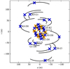 |
Fig. 1 uv-coverage of our observations. Blue crosses represent the data from 2019 March and May, orange crosses represent the data from 2019 June. |
3 Data processing
3.1 Data reduction and calibration
Our data processing consists of the following stages: data reduction, calibration, averaging, and error analysis. In Fig. A.1 we present a flow chart of the general workflow. We reduced the data with the standard MATISSE data reduction pipeline DRS version 1.5.0 (Millour et al. 2016). The pipeline takes the Fourier-transform of the interferograms frame-by-frame, extracts the complex correlated flux for each baseline, and then averages the correlated flux over all frames. The pipeline provides two alternative methods for this averaging, one is the coherent mode, the other is the incoherent mode. The difference is that in coherent mode the average of the correlated fluxes is taken linearly, while in incoherent mode the squared correlated fluxes are averaged. The coherent method needs an estimation for the optical path delay, which is used to correct the phase of the complex correlated flux before averaging. Visibilities are calculated by dividing the averaged correlated flux by the average total flux. For more information we refer to Millour et al. (2016)3. For the L-band data we applied the incoherent method to calculate visibilities. However, in N-band, we used the coherent method to obtain correlated fluxes4. There are several reasons for doing this: (1) L-band correlated flux and total flux data are recorded simultaneously. Therefore, by using visibility, the influence of variable flux levels caused by atmospheric variations is largely eliminated. However, in N-band the photometric exposures are recorded separately from the interferometric ones. This introduces an additional error on the visibility, because of the unknown change in the transfer function between the interferometric and photometric exposures. The size of this uncertainty largely depends on the stability of the atmosphere. (2) The coherent estimator, applied to N-band data, has a significant gain in S/N compared to the incoherent method. In L-band, the coherent and incoherent estimators provide comparable performance. (3) The N-band total flux of our target (Ftot, N ≈ 20 Jy) is below the sensitivity limit of MATISSE with the ATs (Ftot, N = 25−30 Jy), thus N-band visibilities cannot be estimated.
The next step in our data processing is the calibration. For the L-band data we applied the usual visibility calibration as implemented in the DRS. This method can be expressed in the following way:
 (1)
(1)
where V (λ) is the calibrated visibility of the science target, Vraw(λ) is the raw visibility of the science target, and T(λ) is the transfer function derived from the calibrator observation. The transfer function is raw visibility of the calibrator after correcting for its spatial extent. For the N-band data we performed direct flux calibration of the raw correlated fluxes. As this method is not part of the DRS, we developed our own tools to calibrate these data. The direct flux calibration is described by the following equations:

Here Fcorr,ν(λ) is the calibrated correlated flux of the science target,  is the raw correlated flux of the science target, and Tcorr,ν(λ) is the transfer function for flux5. Tcorr, ν(λ) is estimated by dividing the raw correlated flux of the calibrator,
  , by the modeled correlated flux of the calibrator. The latter quantity is calculated as the product of the total spectrum (
 ) and the visibility (Vcal(λ)) of the calibrator. Both
  and Vcal(λ) are usually inferred from fitting stellar atmosphere models to photometric data. We obtained the N-band model spectra of the calibrators (δ Sgr, HD 165135) from the MIDI calibrator database (van Boekel 2004). Vcal (λ) is calculated assuming a uniform disk geometry where the angular diameter of the star is taken from the MDFC. The L- and N-band closure phases were calibrated using the DRS in the frame of the visibility calibration recipe. The calibration results in several calibrated data sets, one for each exposure. To get the final calibrated data we take the average of these data sets.
Proper characterization of the uncertainties in the processed data is highly important for correct interpretation. In Appendix B we perform a detailed quality assessment of the calibrated data. Using the results of this analysis, we exclude the N-band data from May, and all June data from the modeling. This choice is also supported by the evaluation of the L-band transfer function for each of the observing nights shown in Figs. B.1–B.4. Additionally, we set conservative lower limits on the total uncertainties, which are 0.03 for the L-band visibility, 1° for the L-band closure phase, and 8% for the N-band correlated flux6. These values are used in our modeling.
3.2 Final calibrated data
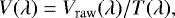
Our final calibrated data sets from 2019 March and May shown in Figs. 2 and 3 consist of the L-band absolute visibilities, the N-band correlated spectra, andthe L- and N-band closure phases7. All these data are spectrally resolved. L-band visibilites ranging from 0.15 (at 132 m baseline) to 0.96 (at 11 m baseline) indicate that the disk is well resolved. The closure phases with the small AT array (Bp < 33 m) are mostly within ± 1°, but on the longer baselines we can see a large signal. These MATISSE closure phases (in the ± 30° range) are significantly larger than the H-band PIONIER ( ± 15°, Kluska et al. 2020) and K-band GRAVITY values ( − 10°... + 4°, GRAVITY Collaboration 2019)8, but smaller thanCHARA K-band closure phases which were found up to 90 degrees (measured at much higher spatial frequencies than the MATISSE data, Setterholm et al. 2018). This closure phase signal indicates that there is a significant departure from centro-symmetry in the L-band brightness distribution at spatial scales <6.4 mas (< 0.7 au) corresponding to the longer baselines (Bp > 56 m). No spectral features (e.g., the 3.3 μm polycyclic aromatic hydrocarbon (PAH) band, arising from C-H stretch resonance) can be seen in the L-band data. Emission from PAHs strongly depends on the ultraviolet radiation field. Unlike the radiative equilibrium attained by (sub-)micron sized dust grains, the absorption and re-emission of radiation by PAHs and very small grains (VSGs) does not correspond to an equilibrium temperature (e.g., Visser et al. 2007). The absence of PAH emission in the spectrum of HD 163296 suggests that the dust grains emitting in the L-band are most likely not PAHs or VSGs, but larger grains in thermal equilibrium. However, the presence of small dehydrogenated grains still cannot be excluded.
The N-band correlated spectra are in the flux range of 10−20 Jy, showing a prominent silicate spectral emission feature. For comparison, we plot a total spectrum measured with the TIMMI2 instrument (van Boekel et al. 2005b) in Fig. 3. The shape of the silicate feature is similar to earlier observations with MIDI (Varga et al. 2018) and Spitzer (Juhász et al. 2012), indicating the presence of large amorphous and various-sized crystalline silicate grains. The shape of most MIDI correlated spectra are similar, suggesting that the crystallinity does not vary significantly with radius. However, the silicate feature is absent from the MIDI correlated spectra on baselines > 74 m (corresponding to a resolution of ϑ < 1.5 au). With the current MATISSE data we cannot probe these spatial scales because the N-band data taken with the large AT-array are unreliable (as described in the previous section). Looking at only the small array MATISSE data, the correlated flux decreases with baseline length, indicating that the object is mildly resolved. We do not see any significant deviation from zero in the N-band closure phases as the signal is quite noisy. We note that the N-band performance of MATISSE is still being assessed, and developments in the data reduction pipeline are expected to increase the N-band data quality.
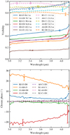 |
Fig. 2 Final L-band calibrated data products from the 2019 March (dashed lines) and May (solid lines) observations: spectrally resolved absolute visibilities (top), and closure phases (bottom). Error bars are indicated at a few random locations. |
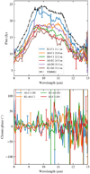 |
Fig. 3 Final N-band calibrated data products from the 2019 March observation (solid lines): correlated spectra (top), and closure phases (bottom). Error bars are indicated at a few random locations. For comparison, we plot the total spectrum on the top panel (dash-dot black line) measured with the TIMMI2 instrument (van Boekel et al. 2005b). |
4 Interferometric modeling
There are two main approaches for the interpretation of IR interferometric data: one is direct image reconstruction and the other is model fitting, either with geometric or radiative transfer models. The first method requires dense uv-sampling, and as we only have uv-points from two telescope configurations, we opt for modeling. Our main goal is to characterize the L- and N-band brightness distributions with simple geometric models by means of deriving some key parameters such as half-light radius, disk orientation, size of the inner cavity, and location of the asymmetry. Simple models are capable of describing the disk emission in a small wavelength range, and therefore we model the L-band and N-band data separately. Additionally, we select different models for the different bands, meaning that each model is best suited to either the L-band or the N-band data set. The models we use in this work are (i) an asymmetric ring model based on Lazareff et al. (2017) (L-band), (ii) an asymmetric flat disk model with inner cavity (L-band), and (iii) a 2D Gaussian model (L- and N-band). All models account for disk inclination and position angle. The ring model and the flat disk model have the same number of free parameters. Stellar flux is also taken into account: the central star is a point at the origin with a fixed flux ratio (f⋆) with respectto the total flux. The model parameters are listed in Table 2 with short explanations.
List of the parameters in our models.
4.1 Asymmetric ring model
As mentioned in Sect. 1, Lazareff et al. (2017) modeled the H-band data of HD 163296 with an asymmetric ring model. In the near-IR, ring models usually work well for Herbig Ae/Be disks, as the bulk of emission comes from the brightly illuminated inner rim of the dust disk. The L-band disk emission could still be dominated by the inner rim. Therefore, the model we adopt in this work, which is based on Lazareff et al. (2017), is an elliptical ring with a first-order azimuthal modulation. The ring is assumed to be centered on the star, and its apparent ellipticity represents its inclination on the sky plane. An azimuthal modulation is introduced to be able to interpret the nonzero closure phases. The model image is convolved with an elliptical pseudo-Lorentzian kernel (Lazareff et al. 2017) to account for the radial thickness of the ring. This model can also represent a centrally peaked brightness distribution if the kernel size is significantly larger than the ring diameter. The fitted parameters are listed in Table 2. A minor difference between our model and that of Lazareff et al. (2017) is the prescription of the azimuthal modulation:
 (4)
(4)
where r is the radius, ϕ is the polar angle, Amod is the amplitude of the modulation, ϕmod is the modulation angle (with respect to the major axis of the ellipse), F0 is the unmodulated image, and Fmod is the modulated image. This is equivalent to the first-order azimuthal modulation (m = 1) in Lazareff et al. (2017). A further difference is that we do not include a spatially extended halo component in our model, as the data do not suggest the presence of such a structure (visibilites at short baselines are very close to 1)9. For more details on the model geometry we refer to Lazareff et al. (2017).
4.2 Flat disk model
As an alternative model to describe the L-band brightness distribution, we apply a physically motivated flat disk geometry based on Menu et al. (2015) and Varga et al. (2018), which has an inner cavity, a sharp inner rim at Rin radius, and a gradually decreasing brightness distribution outside the rim. The brightness distribution is determined by the temperature structure, which has a power-law radial profile. The disk surface emits black-body radiation:
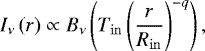 (5)
(5)
where Tin the temperature at the inner radius, and q is the power-law exponent (e.g., Hillenbrand et al. 1992). Following Dullemond et al. (2001), we treat the inner edge of the disk as an optically thick wall, and set Tin to the local black-body equilibrium temperature. In this case, Tin is only dependent on the luminosity of the central star (L⋆):
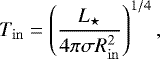 (6)
(6)
where σ is the Stefan–Boltzmann constant. For a discussion on the validity of this formula, we refer to Dullemond & Monnier (2010). We are fitting visibilities, which constrain the shape of the surface brightness distribution but not its absolute level. Therefore, we do not constrain the proportionality factor in Eq. (5). We note that this factor is roughly equivalent to the optical depth of the warm disk surface layer, from which most of the emission we see arises. The model has two parameters describing the structure of the disk, Rin and q. The power-law exponent q accounts for the width of the emitting region. We apply azimuthal modulation in the same way as for the ring model, defined in Eq. (4).
4.3 Two-dimensional Gaussian model
As the object is weakly resolved on the short AT baselines in the N-band, and the corresponding closure phases are consistent with zero signal within the error bars, the previously introduced models cannot be well constrained by the N-band data. Here we require a simple symmetric model with fewer parameters. Thus, we choose a centrally symmetric 2D elongated Gaussian to describe the N-band disk emission. We fit this model to the N-band correlated fluxes. The main fitted parameter is the half width at half maximum of the Gaussian (HWHMGaussian). The total flux of the system (Ftot) is also a fitted parameter. We have three fixed parameters in this model: the flux of the central star (Ftot,⋆), the axis ratio ( cos i), and the position angle of the major axis of the Gaussian (θ), regarded as the disk position angle. The latter two values were taken from ALMA observations (Huang et al. 2018).
We also apply the 2D Gaussian model to the L-band data, with the inclusion of an additional offset point source accounting for asymmetry. This model is described in more detail in the Appendix D.
4.4 Fitting procedure
In order tofind the best-fit parameters, we perform χ2 -minimization. In L-band we calculate the χ2 for the visibilities and for the closure phases separately, and then we sum these two values to get the total χ2 value. We do not apply any weighting to the visibility or the closure phase when calculating the total χ2. By using a simple sum we did not experience any quality difference between the fits to visibilities and the fits to closure phases. In N-band we only calculate the χ2 for the correlated flux.
Our modeling procedure consists of the following steps:
-
First we generate the model image:
-
We create a Cartesian coordinate grid.
-
We then rotate the grid by θ, and scale the coordinates in the x direction by the axis ratio cosi.
-
We generate the brightness distribution on the rotated and scaled grid. Because of the coordinate transform, the isophotes will be ellipses.
-
For the ring and flat disk models, we introduce azimuthal modulation, according to Eq. (4).
-
For the ring model, we convolve the image with an ellipsoidal pseudo-Lorentzian kernel, with a full width at half maximum (FWHM) of the major axis of FWHMkernel. The orientation and axis ratio of the kernel is the same as for the ring.
-
-
We then take the discrete Fourier-transform of the image at the uv-coordinates of the data.
-
We calculate the model visibilities (or correlated fluxes) and closure phases.
-
Finally, we compare the model with the data by estimating χ2.
Optimization of the model parameters is accomplished with a Python implementation of Goodman & Weare’s Markov chain Monte Carlo (MCMC) ensemble sampler, called emcee (Foreman-Mackey et al. 2013a,b). We ran chains of 10 000 steps with 32 walkers. Model parameters are estimated from the MCMC posterior distributions in the following way: in L band, the best-fit values are taken as the mode of the posterior. However, in N-band we use the median for the best fit. In both bands, the uncertainties are taken as the range between the 16th and 84th percentiles. The first 1000 steps in the MCMC chain were discarded when calculating the best-fit values and errors.
List of the best-fit parameters, half-light radii, and χ2-values in our L-band modeling.
5 Results
In the L-band we model the visibilites and closure phases from 2019 March and May. We use the spectral aspect in our data by fitting three wavelengths (3.2, 3.45, 3.7 μm) simultaneously. We average the data in a window of 0.2 μm in width around each fitted wavelength. We fit 36 visibility data points (2 epochs × 3 wavelengths × 6 baselines) and 24 closure phase data points (2 epochs × 3 wavelengths × 4 triangles). The resulting fits are presented in Figs. 4 and 5 for the ring model and flat disk model, respectively.The MCMC posterior distributions are shown in Figs. C.1 (ring model) and C.2 (flat disk model). Table 3 lists the resulting best-fit parameter values. In the modeling, the stellar flux contribution with respect to the total flux is a fixed parameter. For the stellar flux we use the values 0.81, 0.71, and 0.62 Jy at 3.2, 3.45, and 3.7 μm respectively,based on our spectral energy distribution (SED) modeling. The total flux of the star-disk system from MATISSE data is 10.8± 0.8 Jy, with very weak wavelength dependence. Using the stellar and total fluxes we calculate a flux ratio for each of the three wavelengths. The other fixed parameters are the luminosity of the central star L⋆ = 16 L⊙, and the distance of the system d = 101.2 pc, both required only by the flat disk model.
In order to be able to compare the disk sizes resulting from the different modelings, we introduce a half-light radius (Rhl), a single robust measure of the size of the brightness distribution, as follows:
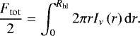 (7)
(7)
This is the usual definition used in the IR interferometry literature (e.g., Leinert et al. 2004; Varga et al. 2018). We note that the stellar flux is not taken into account in the calculation of Rhl. In addition to the ring and flat disk models, we also model the L band emission with a Gaussian plus an additional point source model. The results of this model are presented in Appendix D.
All our models fit the data reasonably well. Comparing the L-band models by the χ2 values, the Gaussian model provides the best fit to the data, although the χ2 values does not differ much between the models. Looking at the best-fit model images, the ring model and the flat disk model give similar brightness distributions. The images show a strongly asymmetric inclined ring with the brightness maximum located at NW. The corresponding position angle (measured from N towards E) is  . In comparison, the additional point source in the Gaussian modeling lies at a similar position angle of 309°. The point source is located at 0.19 au from the center, which is very similar to the value for the inner radius (0.17 au) in the flat disk model. In the ring and flat disk models the ratio of the brightest to faintest surface brightness in the azimuthal variation is 3.5 ± 0.2. In the Gaussian modeling the flux ratio of the additional point source is 0.09± 0.01, which is comparable to the flux contribution of the central star. All three models agree well on the basic geometric parameters: the inclination is
  , the disk position angle is 143° ± 3°, and the half-light radius of theL-band emitting region is 0.33 ± 0.01 au. We note that due to the sparse uv-coverage, which is typical for IR interferometric observations, multiple models with different brightness distributions may also fit the data.
In the N-band, we model the correlated fluxes from 2019 March with the 2D Gaussian model. Five wavelengths between 8.5 and 12.5 μm are fitted independently. Correlated fluxes are averaged in a window of 1 μm in width around each fitted wavelength. There are six fitted data points per wavelength bin. The N-band fit results are shown in Table 4. The half-radii are between 0.89 and 1.34 au, showing an increasing trend with wavelength from 8.5 to 11.5 μm. The N-band emitting region is three to four times larger than the L-band one.
We checked the consistency of our modeling between the two MATISSE bands by extrapolating the best-fit L-band flat disk model to the N-band. The resulting model image calculated at 10.5 μm has a half-light radius of 11.0 mas (1.1 au), which is very close to the value we got from the Gaussian fit to the N-band data (12.3 mas). This result indicates that the flat disk model is capable of broadly representing the disk emission in both MATISSE bands. We also extrapolated the flat disk model to the near-IR in order to make comparisons with PIONIER and GRAVITY observations; this is discussed in the following section.
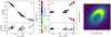 |
Fig. 4 Results of our model fitting for the L-band data with the asymmetric ring model: fits to visibilities against the deprojected baseline length in which the effect of the object inclination is removed (left), fits to closure phases (middle), and the best-fit model image at 3.2 μm (right). Baseline lengths are expressed in spatial frequency units. Data points are indicated by circles, model values by crosses. Left panel: symbols are color coded for the baseline position angle. The blue shaded area on the left panel represents the range of model visibility functions taken at different baseline position angles, at 3.2 μm wavelength. |
List of the fitted and fixed parameters in our N-band modeling with the 2D Gaussian model.
6 Discussion
As mentioned in Sect. 1, discrepancies in the findings of near-IR interferometric studies prevent us from drawing a consistent picture of the inner disk structure of HD 163296. The L-band MATISSE data set is consistent with both ring-like and centrally peaked geometries. The PIONIER model image of Lazareff et al. (2017) and the new GRAVITY reconstructed images (GRAVITY Collaboration, in prep.) show an asymmetric ring. However, the recent directly reconstructed PIONIER image (Kluska et al. 2020) is centrally peaked. Kluska et al. (2020) performed an image-reconstruction simulation on the best-fit ring model of Lazareff et al. (2017) by calculating synthetic interferometric observables from the model image, and found that the reconstructed image on the synthetic data set is in agreement with the reconstructed image on the real data set. This indicates that the presence of a central cavity is plausible, and the ambiguity in the image reconstruction may be caused by the insufficient resolution. In a K-band interferometric study of a sample of Herbig Ae/Be stars, including HD 163296, a ring model based on Lazareff et al. (2017) was fitted (GRAVITY Collaboration 2019). The best-fitting model to HD 163296 is dominated by the centrally peaked component. Similarly, Setterholm et al. (2018) found that a simple Gaussian fits better than a thin ring or uniform disk to H- and K-bands interferometric data. It is important to note that neither GRAVITY Collaboration (2019) nor Setterholm et al. (2018) modeled closure phases, and so their models are symmetric. Further interferometric observations with optimized uv-coverage at the longest possible baselines are needed to properly resolve the disk structure within r = 0.3 au. The VLTI currently provides baseline lengths up to ~130 m, but there are ongoing efforts to open the longest AT baseline (220 m). Having such a long baseline could provide highly valuable constraints on the inner disk structure.
Our results for the disk inclination and position angle are in line with earlier near-IR interferometric observations (i =45°−50°, θ = 126°−134°), with ALMA observations (i = 47°, θ = 133°), and with SPHERE observations (θ = 134°−137.5°) (Lazareff et al. 2017; Kluska et al. 2020; GRAVITY Collaboration 2019; Setterholm et al. 2018; Huang et al. 2018; Isella et al. 2018; Muro-Arena et al. 2018). Therefore, we conclude that the inner disk of HD 163296 is well aligned with the outer disk.
6.1 The nature of the asymmetry
A circumstellar disk seen at an inclined viewing angle can show brightness asymmetries even if the structure of the disk is perfectly circularly symmetric. These asymmetries arise from radiative transfer effects. An example is the anisotropic scattering of the stellar light (e.g., Pinte et al. 2009). In the case of HD 163296, the star contributes less than 7% to the total L-band flux, and therefore scattered light is negligible in the disk emission. A further inclination effect is that the far side of the inner rim appears brighter than the (self-shadowed) near side10 (e.g., Isella & Natta 2005). In both scenarios the brightness maximum should correspond to the position angle of the minor axis of the projected image. Surprisingly, our MATISSE results show that the maximum brightness in the inner disk of HD 163296 is towards the semimajor axis to the NW. This is not compatible with inclination effects, and therefore we argue that the asymmetry is caused by an azimuthal variation in the disk structure, or in the dust properties (like grain size).
In the PIONIER model image of Lazareff et al. (2017), the position angle of the brightness maximum is 273° (measured from N towards E). This is 65° away from the position angle we get from MATISSE data ( ) using the asymmetric ring model which was also used for the PIONIER modeling. Furthermore, GRAVITY Collaboration (in prep.) report that the position angle of the bright arc has changed from ≈ 60° to ≈ 240° between 2018 July and 2019 July. All evidence indicates a time-variable morphology for the r < 0.3 au disk region. Detecting the variable morphology from MATISSE data alone is challenging, because the data sets taken on the short baselines (three out of the four observations) are barely sensitive to the asymmetries as the closure phases are within ± 1°. Nevertheless, we tried to detect the change in the position of the asymmetry between the 2019 March and May MATISSE epochs by fitting the corresponding data sets independently. We used the flat disk model by fixing all parameters to their best-fit values, except for Amod and ϕmod. For 2019 March, we get
  (measured from the major axis), and for 2019 May we get ϕmod = 179.5° ± 2°. The difference is not significant. We estimate that the orbital periods at the observed radius range (0.18−0.33 au) of the ring range from 20 to 50 days. The temporal coverage of the interferometric data (from MATISSE, PIONIER, and GRAVITY) does not allow us to constrain the rotation period.
The physical origin of the time-variable disk structure is unclear. Several kinds of magne to hydrodynamic instabilities (e.g., Flock et al. 2015, 2017), as well as Rossby wave instability (Lovelace et al. 1999; Meheut et al. 2010)and gravitational instability (e.g., Durisen et al. 2007; Kratter & Lodato 2016) can produce such asymmetric disk features. Alternatively, a (sub)stellar companion (e.g., Brunngräber & Wolf 2018; Szulágyi et al. 2019)could also be the direct cause of the asymmetry. Our Gaussian plus additional point source model can provide constraints on the flux of such a putative companion. The offset point source in this model has an L-band flux of 0.9 Jy. We also fitted a physically more realistic model which has two point sources (the central star and the companion), and a circumbinary ring. The ring geometry is the same as the one we used in the smoothed ring model, except that the circumbinary ring is symmetric. This model predicts an even higher flux for the companion (1.5 Jy). These results imply that the companion should be brighter than the central star in the L-band, the latter having a flux of ~0.7 Jy. The separation of the companion from the central star in the circumbinary ring model is ~ 0.15 au. In order to get constraints on the near-IR flux of the putative companion, we fitted the PIONIER data from Lazareff et al. (2017) with the Gaussian plus additional point source model, and also with the circumbinary ring model. The H-band fluxes we get for the companion are in the range of 0.2−0.4 Jy, assuming a total H-band flux for the system of 6.4 Jy, and a H-band stellar flux of 2.5 Jy.
If the object causing the asymmetry is a stellar companion, its near-IR flux is very likely to be higher than its L-band flux. Our interferometric modeling suggests that this is not the case. If we assume that the companion is a planet, its close location to the star in addition to its high flux would classify it as a hot Jupiter. Hot-start planet models (e.g., Spiegel & Burrows 2012) predict that a young planet with a mass of 10 M♃ may have an effective temperatureof around 2500 K and a radiusof 2.3 R♃. The IR flux from such planet itself would be too small (a few mJy in L-band) to explain our observations. We also consider that the IR emission originates from a circumplanetary disk. If we assume optically thick thermal dust emission (with a dust temperature of 1500 K), the required L-band flux could be provided by a disk with a diameter of ~0.1 au. However, the Hill-sphere diameter of a 10 M♃ mass planet located at r = 0.15 au is 0.035 au (assuming a stellar mass of 1.9 M⊙), which is too small to accommodate a circumplanetary disk of the required size. Although a much hotter circumplanetary material filling the Hill-sphere might provide enough L-band flux to match the MATISSE observations, its near-IR flux contribution would be much larger and thus incompatible with the PIONIER data. Therefore, we argue that the observed brightness asymmetry is caused by an asymmetric structure in the disk itself.
Hydrodynamic instabilities may be responsible for the disk asymmetry we see in our data. In order to test the plausibility of the Rossby wave instability hypothesis, we performed hydro-dynamical numerical simulations with AMRVAC11 (Xia et al. 2018) of the inner edge of the disk (see also Robert et al. 2020a for the setup). Only the dynamical evolution of the gas is modeled and the dust is considered to follow the gas. This is valid for small dust grains with a Stokes number of  , where s is the size of the dust grain, ρd its internal density, and Σg the gas surface density. The strong density gradient at the inner edge of the disk creates a minimum in the vortensity (or potential vorticity) profile. This is unstable due to the Rossby wave instability that form vortices (Lovelace et al. 1999). An inverse cascade in this 2D simulation is eventually responsible for the survival of a unique large-scale vortex; a similar evolution would be obtained within a thin 3D disk (Meheut et al. 2012a). This anticyclone is a region of high pressure and density, as can be seen in Fig. 6, which is known to concentrate dust (Barge & Sommeria 1995). Although neither the gas nor the vortex rotate at the local Keplerian frequency, in both cases the difference from Keplerian rotation is small. Thus, Keplerian motion is a good approximation for the variability timescale in the vortex scenario. For further details on the dynamical signatures of vortices we refer to Robert et al. (2020b).
Density enhancement alone is not expected to increase the surface brightness of the vortex region, assuming optically thick emission. What is required to produce increased radiation, is a change in the dust properties. A potential mechanism for that is the production of small grains by grain collisions which also increase the local temperature. The combined effect of more small grains and increased temperature will be a local increase in surface brightness. Such a mechanism could be an explanation for the asymmetric feature in HD 163296. The azimuthal extent of the vortex roughly corresponds to that of the asymmetry in our ring and flat disk model images, although in our modeling we only applied first-order azimuthal modulation. To fully test this hypothesis, a hydrodynamical simulation including the dust dynamics is needed, as the Stokes number of solids of a given size strongly varies at the edge of a disk due to the gas surface density profile. This hydrodynamical simulation should then be coupled to radiative transfer code to provide synthetic images and synthetic interferometric observables.
Rich et al. (2020) report Hubble Space Telescope (HST) coronagraphic imaging of HD 163296, and multiwavelength photometric monitoring from 2016-2018. These latter authors found azimuthally asymmetric surface brightness variations between the HST epochs, and they conclude that the disk illumination varies on timescales of less than 3 months. They suggest that the origin of the brightness variations is shadowing by a structure residing within a radius of 0.5 au. This result fits well in our picture of the variable inner disk morphology, and it may also support our vortex scenario. In previous 3D vortex simulations it was found that the disk is vertically more extended at the location of the vortices (Meheut et al. 2012b). Thus, a vortex can indeed be a source of shadowing.
To shed more light on the origin of the asymmetry, it would be highly important to measure its rotation period. For this, monitoring observations with a cadence of a few days to a week are needed. Coordinated observations using near- and mid-IR interferometric instruments (e.g., GRAVITY and MATISSE) quasi-simultaneously are also desired in order to reveal the chromatic nature of the asymmetry, and to improve the quality of the reconstructed images (Sanchez-Bermudez et al. 2018). The assessment of the chromaticity can help to constrain the physical nature of the asymmetry.
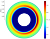 |
Fig. 6 Gas surface density at the inner edge of a disk obtained with numerical simulation. The asymmetry in density is due to a vortex formed by the Rossby wave instability. |
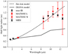 |
Fig. 7 Characteristic size of the emitting region as function of wavelength. The red points are derived from our MATISSE data. The 1.6 and 2.2 μm points come from PIONIER (Lazareff et al. 2017; Kluska et al. 2020) and GRAVITY (GRAVITY Collaboration 2019) observations, respectively. Black crosses represent our new fits to MIDI data published by Varga et al. (2018). The solid line is from the DIANA radiative transfer model of HD 163296 (Woitke et al. 2019). The dashed line corresponds to our flat diskmodel. |
6.2 The size of the IR-emitting region
In Fig. 7 we show the half-light radius of the disk derived from near- and mid-IR interferometric observations as function of wavelength. The new L-band size from our observations is very close tothe K-band size, suggesting that the near-IR and the 3−4 μm emissions originate from the same disk region. There is a general increasing trend of the half-light radius with wavelength. This is because towards longer wavelengths we become sensitive to material at lower temperatures located further from the central star. In the N-band, the characteristic size of the disk emission as traced with our MATISSE data (red crosses) and archival MIDI data (black crosses) is much larger than at shorter wavelengths. Furthermore, the apparent size in the 10 μm silicate feature is somewhat larger than in the adjacent continuum. This behavior is expected based on radiative transfer calculations (van Boekel et al. 2005a): the emissionin the N-band arises in part from the warm surface layer and in part from the cooler (and hence at a given wavelength apparently more compact) disk interior. In the N-band, the warm surface layer is optically thin in the vertical direction. Therefore, the relative contribution of the spatially more extended surface layer emission follows its opacity curve, which explains both why we see an emission feature and why the spatial extent of the emission is highest in the emission band.
In Sect. 5 we demonstrate that our best-fitting flat disk model to the L-band data is capable of reproducing the observedincrease in size between L- and N-band. However, we note that this model does not include the effects of the silicate opacity. As can be seen in Fig. 7, the flat disk model (representedby the dashed line) is also in good agreement with the disk sizes measured by PIONIER and GRAVITY in the near-IR. We note that the H- and K-band sizes found by Setterholm et al. (2018) were the same within errors as the longer CHARA baselines.
To compare our N-band results with older MIDI observations, we fitted the same 2D Gaussian models that we used for MATISSE data to MIDI data taken from Varga et al. (2018). The resulting N-band disk sizes from MIDI are plotted in Fig. 7 (black crosses). The N-band sizes derived from MATISSE and MIDI observations are in good agreement. The error bars on the MATISSE N-band data points are much larger than those on the MIDI points. We attribute this to the following two factors: (1) the MIDI data set has many more data points (27 MIDI vs. 6 MATISSE correlated flux points), and (2) the MIDI data set samples a larger range of spatial scales (1 au < ϑ < 9 au) than MATISSE (3 au < ϑ < 10 au). These two factors enable more precise size measurements for the MIDI data.
For comparison, we overplot a size-wavelength curve from a radiative transfer modeling of HD 163296 in Fig. 7. The disk model is taken from the DIANA project website12 (Woitke et al. 2019). We used the radiative transfer code MCMax (Min et al. 2009) to generate images of the disk at different wavelengths. We calculated the half-light radius including the stellar flux contribution, and used circular apertures. The half-light radii of the DIANA disk model are in agreement with H-, K-, and L-band observations, but the observed N-band sizes are significantly larger than the model values. A possible explanation for this difference is that the dust grain size distribution changes with the distance from the star, that is, the innermost disk lacks small ( < 2−5 μm) silicate grains, whilst slightly further away (at ~ 1 au) small grains are still abundant. Millan-Gabet et al. (2016) found similar results for a number of Herbig Ae/Be stars, by using a two-rim model which provided a better fit to IR interferometric and SED data compared to an inner rim plus flared disk geometry. The model of these latter authors featured an inner rim with large grains, and an outer rim with larger scale height containing smaller grains. The inferred inner rim radius for HD 163296 (0.39 au) seems to be incompatible with our L-band half-light radius, but their outer rim radius (1.1 au) is a close match to our N-band half-light radii.
Further evidence for this scenario might come from interferometric modeling. We fitted the MIDI data from Varga et al. (2018) with the flat disk temperature gradient model at three wavelengths (8, 10.7, and 13 μm). The fits at 8 and 10.7 μm, representingthe continuum emission, are consistent with a continuous disk beginning at the dust sublimation radius, while at 10.7 μm, which is in the middle of the silicate feature, the data are better represented by a disk with an inner hole (with ~ 0.6 au inner radius). Thus, it is likely that the structure of the N-band continuum emission is continuous, while the silicate emission comes from a larger region exhibiting an inner gap. A strong N-band silicate feature is only expected from small (<1 μm) silicate grains. Thus, a radial change in the grain size distribution, probably due to grain growth in the innermost disk, naturally explains our findings. This scenario was found to be the case for the transitional disk T Cha (Olofsson et al. 2013).
An alternative solution for the larger-than-expected N-band sizes could be the presence of dust in a halo-like structure. Ellerbroek et al. (2014) studied optical to near-IR spectra of the jet of HD 163296. These latter authors detected fadings in the optical which coincided with near-IR brightenings, and propose that this can be explained by dust lifted high above the disk plane in a disk wind launched at ≳ 0.5 au radii. Such optically thin dust cloud above the disk might also be consistent with our results. While our analysis with simple geometric models provides valuable insights intothe N-band disk structure, to reach a consistent multiwavelength view on the dust distribution, more detailed modeling is needed.
6.3 The nature of the dust sublimation zone
The dust sublimation zone is not an abrupt boundary between the innermost gaseous disk and the dusty disk regions, but rather a continuous transition region (e.g., Isella & Natta 2005; Kama et al. 2009; Dullemond & Monnier 2010). The location and properties of this region heavily depend on the grain sizes and composition. To estimate a radial range for the dust sublimation zone of HD 163296, we apply Eq. (9) from Dullemond & Monnier (2010). This equation contains the factor ϵ which is expressed by dividing the effectiveness of the emission at the wavelength at which the dust radiates away the heat with that of the absorption at the wavelength of the stellar emission. It represents how efficiently the dust cools. We assume a sublimation temperature of 1500 K, a stellar luminosity of 16 L⊙, and a range for the cooling efficiency factor of 0.1 < ϵ < 1.0. This yields a wide radial range of 0.14−0.43 au for the sublimation zone. Our flat disk model features a sharp inner rim, but this is likely not a physically realistic representation of the sublimation zone. Because of the sparse uv-coverage and insufficient resolution, we cannot recover the radial brightness profile of the dust sublimation zone from the data. Nevertheless, our modeling results may provide some hints as to the location. The radius of the inner rim in our flat disk model is 0.18 au, which is close to the lower limit of the estimated radial range for the sublimation zone. Furthermore, in our ring model the disk surface brightness near the star is still 20% of the value at the brightness maximum. Both models suggest that a non-negligible fraction of the mid-IR light comes from a region where μm-sized grains may not survive. Considering Eq. (9) of Dullemond & Monnier (2010), we consider the following solutions for this issue. The first is the presence of large (≳ 10 μm) dust grains which have a high cooling efficiency factor (ϵ ≈ 1). At 0.18 au radius these large grains would have a temperature of only 1300 K. The second solution is the presence of small grains made of refractory materials which have a higher sublimation temperature. A refractory grain with ϵ ≈ 0.1 at 0.18 au should endure a temperature of 2300 K. Additionally, gas emission within the dust sublimation radius might contribute to the near- and mid-IR radiation.
In the following we discuss these three scenarios in the following order: gas emission, refractory grains, and large grains. Several studies have proposed that gas continuum emission inside the dust sublimation radius can provide a significant contribution to the near-IR radiation of protoplanetary disks (e.g., Muzerolle et al. 2004; Eisner et al. 2007a; Isella et al. 2008; Weigelt et al. 2011). Tannirkulam et al. (2008) successfully modeled K-band interferometric data of HD 163296 using a rim model with an additional uniform disk component in the inner cavity attributed to gas continuum emission. Benisty et al. (2010) performed radiative transfer modeling of HD 163296 using AMBER H- and K-bands observations, and found a good fit to the data with a model where the disk emission originates from a region between 0.1 and 0.45 au. These latterauthors tested an accretion disk model with gas in local thermodynamic equilibrium (LTE), a nonLTE model of thin layers of gas in the disk atmosphere, and a model with hot gas (T = 8000 K). However, they found that these gas models are inconsistent with observational data.
Benisty et al. (2010) propose instead the presence of refractory dust grains in the 0.1−0.45 au region. How dust can survive the high interior temperatures (2100−2300 K) is not well established. From the dust types they discuss, iron seems to be a good candidate. However, thermal equilibrium calculations show that above 1500 K only Al- and Ca-bearing minerals persist, and Fe-containing grains are no longer stable (e.g., Scott 2007). One of the most refractory minerals known is corundum (Al2O3), which is stable up to ~ 1800 K. The existence of refractory dust in the disk of HD 163296 that sublimates at ~ 1850 K was also proposed by Tannirkulam et al. (2008). As an additional scenario, we consider the presence of large dust grains in the inner disk. Large silicate grains have a large cooling efficiency, and so they can survive at a distance from the star similar to small refractory grains. The depletion of small grains in the inner disk is also supported by our findings regarding the structure of the N-band-emitting region discussed in Sect. 6.2. Testing the plausibility of these scenarios requires more detailed modeling, which is not in the scope of this paper.
7 Summary
Here we present the first MATISSE observations of the disk around the Herbig Ae/Be star HD 163296. The object is resolved both in L- and N-bands. The L-band closure phases indicate significant brightness asymmetry. We modeled the disk using various geometric models, including an asymmetric ring, an asymmetric flat disk with inner cavity, and a 2D Gaussian. All three geometries were used to model the L-band disk structure, while only the last was fitted to the N-band data. Our main findings are as follows:
- 1.
Our models can describe the L-band visibilities and closure phases well. The half-light radius of the L-band-emitting region is 0.33 ± 0.01 au, the inclination is
 , and the position angle is 143° ± 3°.
 - 2.
The N-band-emitting region has a half-light radius of 0.9−1.3 au, showing an increasing trend with wavelength from 8.5 to 11.5 μm. The observed N-band sizes are significantly larger than the prediction from a radiative transfer model. A possible explanation for this difference is the lack of small silicate grains in the inner disk regions (r ≲ 0.6 au).
- 3.
The size of the L-band-emitting region is very similar to the near-IR sizes, and three to four times smaller than the N-band size. This suggests that the same emission component dominates the disk emission from the near-IR wavelengths to the L-band.
- 4.
There is no significant misalignment of the L-band-emitting disk region with respect to near-IR and mm (ALMA) measurements.
- 5.
Our modeling reveals a significant brightness asymmetry in the L-band disk emission. The brightness maximum of the asymmetry is located at the NW part of the disk image, nearly at the position angle of the semimajor axis. The position of the brightness asymmetry suggests that it is caused by a variation in the disk structure in or near the inner rim.
- 6.
Comparing our result on the location of the asymmetry to PIONIER (Lazareff et al. 2017) and GRAVITY (GRAVITY Collaboration, in prep.) results, we find that the morphology of the r < 0.3 au disk region is time-variable. We propose that the asymmetric structure orbits the star with a period of ~ 20−50 days.
- 7.
The physical origin of the rotating asymmetry is unclear. We tested a hypothesis where a vortex created by Rossby wave instability causes the asymmetry. We find that a unique large-scale vortex may be compatible with our data. Further hydro-dynamical simulations and radiative transfer modeling are needed to fully evaluate this scenario.
- 8.
Our models predict that a non-negligible fraction of the L-band disk emission originates inside the dust sublimation radius for μm-sized grains. For the origin of this emission, we consider the presence of refractory grains and large (≳10 μm-sized) grains.
Acknowledgements
MATISSE was designed, funded and built in close collaboration with ESO, by a consortium composed of institutes in France (J.-L. Lagrange Laboratory – INSU-CNRS – Côte d’Azur Observatory – University of Côte d’Azur), Germany (MPIA, MPIfR and University of Kiel), the Netherlands (NOVA and University of Leiden), and Austria (University of Vienna). The Konkoly Observatory and Cologne University have also provided some support in the manufacture of the instrument. This research has made use of the services of the ESO Science Archive Facility. The research of J. Varga and M. Hogerheijde is supported by NOVA, the Netherlands Research School for Astronomy. T.H. acknowledges support from the European Research Council under the Horizon 2020 Framework Program via the ERC Advanced Grant Origins 83 24 28. A.G. acknowledges support from the European Research Council (ERC) under the European Union’s Horizon 2020 research and innovation programme under grant agreement No 695099 (project CepBin). P.A. acknowledges support from the Hungarian NKFIH OTKA grant K132406, and from the European Research Council (ERC) under the European Union’s Horizon 2020 research and innovation programme under grant agreement No 716155 (SACCRED). We all would like to thank our colleagues and friends, Olivier Chesneau, Michel Dugué, J. Alonso, A. Glazenborg, H. Hanenburg, J. Idserda, T. Phan Duc, and K. Shabun for their contributions to MATISSE.
Appendix A Data processing flow chart
Figure A.1 shows a flow chart of our data processing workflow.
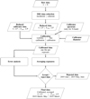 |
Fig. A.1 Flow chart of our data processing workflow. V indicates visibility, CP indicates closure phase, and Fcorr indicates correlated flux. |
Appendix B Error analysis
The aim of this section is to assess the uncertainty of the calibrated data products. The MATISSE pipeline estimates errors by dividing a raw exposure into chunks, and reducing these chunks separately. The error is then taken as the standard deviation of the reduced data in the chunks. This estimation accounts for the instrument-related noise sources. However, a more significant source of error is our incomplete knowledge of the transfer function. During the typically 20− 30 min time-lag between a science and calibrator observation, the atmospheric conditions could change a lot, so the transfer function varies significantly. This error causes an uncertainty in the overall visibility or flux level of the spectrum, and therefore is systematic in nature. In Figs. B.1–B.4 we plot the L-band transfer function over time for each night, for each baseline, and for each BCD configuration. To assess the uncertainties in the calibrated data we employ the following:
-
We estimate the random noise (σr) by subtracting the trend from the data, and taking the standard deviation of the residual signal. This error is the uncorrelated noise between the spectral channels.
-
We estimate short-term systematic uncertainties (σsys,s) by taking the standard deviation of the four or eight exposures taken during the interferometric observation13. The characteristic time scale corresponding to σsys,s is 4−8 min.
-
We estimate long-term systematic uncertainties (σsys,l) by calibrating the science data with alternative calibrators. One calibrator is chosen before, the other after the science observation. Thus we have three calibrated data sets: one with the original calibrator, and two with the alternative calibrators. Then we take the standard deviation of these data sets. The characteristic time scale corresponding to σsys,s is 1−3 h.
The average uncertainties (averaged over baselines and wavelengths) are listed in Table B.1 for each of the four observations. For N-band we show the relative errors on the correlated flux. For the L-band visibility and for the N-band correlated flux systematic uncertainties are larger than the random noise. Comparing the systematic errors, we see that σsys,l > σsys,s, indicating that hour-long variations of the atmosphere are larger than changes over a few minutes. The values for σsys,l in L-band are consistent with the scatter in the transfer function values, shown in the captions of the Figs. B.1–B.4. We note that the May data set has the smallest absolute errors on visibility, but in relative terms the March data set is better. The origin of this difference is that the May data set has significantly lower L-band visibilities (compared to the March data). In relative terms the March data has σsys,l values of ≈ 2%, while the corresponding values for the May data are in the range of 2−6%.
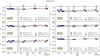 |
Fig. B.1 L-band transfer function during the night from 2019-03-22 to 2019-03-23. Gray shading indicates the observation time of HD 163296.The gray lines, one for each BCD configuration, are cubic polynomial fits to the points. In the captions, σ is the relative standard deviation of the transfer function values. |
Error statistics of our observations.
In the closure phases, the largest uncertainty is the σsys,s, which actually reflects instrumental effects (revealed by the beam commutation), not atmospheric variations. Averaging the exposures suppresses the instrumental noise, and results in greatly reduced systematic uncertainties. Furthermore, σsys,l < σsys,s, indicating that the variable atmosphere has a smaller impact on the closure phase uncertainty, than the instrumental effects. The most significant error source on the closure phase which remains after averaging the exposures is the random noise (σr). It is still within 1° in L-band, but quite large (>20°) in N-band. As a summary for Table B.1, the overall uncertainty in L-band visibility is < 0.02 for the March and May data (taken in very good weather), and >0.06 for the June data which was recorded under unfavorable atmospheric conditions. For the N-band correlated flux the overall uncertainty is <8% for the March data, and ~20% for the Junedata.
The June data sets are generally consistent with the March data, but having significantly larger uncertainties. As the baselines probed in March and June were very similar (on the small AT array), there is little added value of including the lower quality June data in the modeling. Thus, we do not use these data in our analysis at all. Additionally, the N-band data from May suffers from a bias affecting the correlated flux at flux levels close to the instrument sensitivity limit (5− 8 Jy with ATs). The correlated fluxes of HD163296 at ≳50 m baselines probed in May, based on earlier VLTI/MIDI observations, are expected to be less than 8 Jy (Varga et al. 2018). Due to the bias we are unable to provide error estimates for the May N-band correlated fluxes, and we do not use these data in this study.
When calculating our final averaged calibrated data we assign an uncertainty to each data point by combining the error provided by the MATISSE pipeline andour σsys,s estimate. Thus, long-term systematics are not included in the error bars. Additionally, our error analysis does not encompass errors caused by the uncertainty in the calibrator diameter, and errors due to the uncertainty in the calibrator model spectrum. For our modeling we set conservative lower limits on the total uncertainties, which are 0.03 for the L-band visibility, 1° for the L-band closure phase, and 8% for the N-band correlated flux.
Appendix C Posterior distributions
Figures C.1 and C.2 show the posterior distributions of the MCMC chain for the smoothed ring model and flat disk model, respectively.
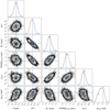 |
Fig. C.1 Posterior distributions for the smoothed ring model in L-band from our MCMC sampling. Blue lines represent the best-fit values. |
Appendix D Additional modeling
In order to explore whether a centrally symmetric model could fit the L-band data, we apply a model featuring a central 2D elliptical Gaussian. The central star, as in the previous L-band models, is represented as a point source, with a fixed flux ratio. To account for asymmetry, we add a component that can be at an offset position. We first experimented with models where we used a Gaussian blob for the additional component. In these models the fitting converged towards a very small size for the Gaussian, without constraining a lower limit for the size. Thus, we choose to represent the additional component as a point source. This model has six fitted parameters, just like our other models for the L-band. The central Gaussian is modeled with the following three parameters: the half width at half maximum size (HWHMGaussian), the axis ratio ( cos i), and the position angle of the majoraxis (θ). The remaining three parameters are the coordinates of the additional point source (xδ, yδ), and its flux ratio with respect to the whole circumstellar emission (fδ).
The fitting procedure was the same as described in Sect. 4.4. The resulting fits are presented in Fig. D.1, and the corresponding posterior distributions are shown in Fig. D.2. The fitted parameters are listed in Table D.1.
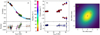 |
Fig. D.1 Same as Fig. 4, but with the Gaussian plus point source model. Panel c: indicate the locations of the central star (star symbol) and of the additional point source (circle). |
List of the best-fit parameters, half-light radii, and χ2-values in the Gaussian L-band modeling.
References
- Andrews, S. M., Huang, J., Pérez, L. M., et al. 2018, ApJ, 869, L41 [Google Scholar]
- Avenhaus, H., Quanz, S. P., Garufi, A., et al. 2018, ApJ, 863, 44 [Google Scholar]
- Bailer-Jones, C. A. L., Rybizki, J., Fouesneau, M., Mantelet, G., & Andrae, R. 2018, AJ, 156, 58 [NASA ADS] [CrossRef] [Google Scholar]
- Barge, P., & Sommeria, J. 1995, A&A, 295, L1 [NASA ADS] [Google Scholar]
- Benisty, M., Natta, A., Isella, A., et al. 2010, A&A, 511, A74 [NASA ADS] [CrossRef] [EDP Sciences] [Google Scholar]
- Brunngräber, R., & Wolf, S. 2018, A&A, 611, A90 [NASA ADS] [CrossRef] [EDP Sciences] [Google Scholar]
- Burtscher, L., Meisenheimer, K., Tristram, K. R. W., et al. 2013, A&A, 558, A149 [NASA ADS] [CrossRef] [EDP Sciences] [Google Scholar]
- Cruzalèbes, P., Petrov, R. G., Robbe-Dubois, S., et al. 2019, MNRAS, 490, 3158 [Google Scholar]
- Devine, D., Grady, C. A., Kimble, R. A., et al. 2000, ApJ, 542, L115 [Google Scholar]
- Dullemond, C. P., Dominik, C., & Natta, A. 2001, ApJ, 560, 957 [Google Scholar]
- Dullemond, C. P., & Monnier, J. D. 2010, ARA&A, 48, 205 [Google Scholar]
- Durisen, R. H., Boss, A. P., Mayer, L., et al. 2007, Protostars and Planets V, eds. B. Reipurth, D. Jewitt, & K. Keil (Tucson, AZ: University of Arizona Press), 607 [Google Scholar]
- Eisner, J. A., Chiang, E. I., Lane, B. F., & Akeson, R. L. 2007a, ApJ, 657, 347 [Google Scholar]
- Eisner, J. A., Hillenbrand, L. A., White, R. J., et al. 2007b, ApJ, 669, 1072 [NASA ADS] [CrossRef] [Google Scholar]
- Ellerbroek, L. E., Podio, L., Dougados, C., et al. 2014, A&A, 563, A87 [NASA ADS] [CrossRef] [EDP Sciences] [Google Scholar]
- Flock, M., Fromang, S., Turner, N. J., & Benisty, M. 2017, ApJ, 835, 230 [Google Scholar]
- Flock, M., Ruge, J. P., Dzyurkevich, N., et al. 2015, A&A, 574, A68 [NASA ADS] [CrossRef] [EDP Sciences] [Google Scholar]
- Foreman-Mackey, D., Conley, A., Meierjurgen Farr, W., et al. 2013a, emcee: The MCMC Hammer [Google Scholar]
- Foreman-Mackey, D., Hogg, D. W., Lang, D., & Goodman, J. 2013b, PASP, 125, 306 [Google Scholar]
- GRAVITY Collaboration (Perraut, K., et al.) 2019, A&A, 632, A53 [NASA ADS] [CrossRef] [EDP Sciences] [Google Scholar]
- Hillenbrand, L. A., Strom, S. E., Vrba, F. J., & Keene, J. 1992, ApJ, 397, 613 [Google Scholar]
- Huang, J., Andrews, S. M., Dullemond, C. P., et al. 2018, ApJ, 869, L42 [Google Scholar]
- Isella, A., Huang, J., Andrews, S. M., et al. 2018, ApJ, 869, L49 [Google Scholar]
- Isella, A., & Natta, A. 2005, A&A, 438, 899 [NASA ADS] [CrossRef] [EDP Sciences] [Google Scholar]
- Isella, A., Tatulli, E., Natta, A., & Testi, L. 2008, A&A, 483, L13 [NASA ADS] [CrossRef] [EDP Sciences] [Google Scholar]
- Jamialahmadi, N., Lopez, B., Berio, P., et al. 2018, MNRAS, 473, 3147 [Google Scholar]
- Juhász, A., Dullemond, C. P., van Boekel, R., et al. 2012, ApJ, 744, 118 [Google Scholar]
- Kama, M., Min, M., & Dominik, C. 2009, A&A, 506, 1199 [NASA ADS] [CrossRef] [EDP Sciences] [Google Scholar]
- Kluska, J., Berger, J. P., Malbet, F., et al. 2020, A&A, 636, A116 [CrossRef] [EDP Sciences] [Google Scholar]
- Kluska, J., García López, R., & Benisty, M. 2016, Proc. SPIE, 9907, 99070V [Google Scholar]
- Kratter, K., & Lodato, G. 2016, ARA&A, 54, 271 [Google Scholar]
- Kraus, S., Hofmann, K. H., Malbet, F., et al. 2009, A&A, 508, 787 [NASA ADS] [CrossRef] [EDP Sciences] [Google Scholar]
- Kraus, S., Ireland, M. J., Sitko, M. L., et al. 2013, ApJ, 768, 80 [Google Scholar]
- Lazareff, B., Berger, J.-P., Kluska, J., et al. 2017, A&A, 599, A85 [NASA ADS] [CrossRef] [EDP Sciences] [Google Scholar]
- Leinert, C., van Boekel, R., Waters, L. B. F. M., et al. 2004, A&A, 423, 537 [NASA ADS] [CrossRef] [EDP Sciences] [Google Scholar]
- Lopez, B., Lagarde, S., Jaffe, W., et al. 2014, The Messenger, 157, 5 [NASA ADS] [Google Scholar]
- Lovelace, R. V. E., Li, H., Colgate, S. A., & Nelson, A. F. 1999, ApJ, 513, 805 [Google Scholar]
- Matter, A., Labadie, L., Augereau, J. C., et al. 2016a, A&A, 586, A11 [NASA ADS] [CrossRef] [EDP Sciences] [Google Scholar]
- Matter,A., Lagarde, S., Petrov, R. G., et al. 2016b, Proc. SPIE, 9907, 990728 [Google Scholar]
- Matter, A., Lopez, B., Antonelli, P., et al. 2016c, Proc. SPIE, 9907, 99070A [Google Scholar]
- Meheut, H., Casse, F., Varniere, P., & Tagger, M. 2010, A&A, 516, A31 [NASA ADS] [CrossRef] [EDP Sciences] [Google Scholar]
- Meheut, H., Keppens, R., Casse, F., & Benz, W. 2012a, A&A, 542, A9 [Google Scholar]
- Meheut, H., Meliani, Z., Varniere, P., & Benz, W. 2012b, A&A, 545, A134 [NASA ADS] [CrossRef] [EDP Sciences] [Google Scholar]
- Menu, J., van Boekel, R., Henning, T., et al. 2014, A&A, 564, A93 [NASA ADS] [CrossRef] [EDP Sciences] [Google Scholar]
- Menu, J., van Boekel, R., Henning, T., et al. 2015, A&A, 581, A107 [NASA ADS] [CrossRef] [EDP Sciences] [Google Scholar]
- Millan-Gabet, R., Che, X., Monnier, J. D., et al. 2016, ApJ, 826, 120 [Google Scholar]
- Millour, F., Berio, P., Heininger, M., et al. 2016, SPIE Conf. Ser., 9907, 990723 [Google Scholar]
- Millour, F., Petrov, R. G., Vannier, M., & Kraus, S. 2008, SPIE Conf. Ser., 7013, 70131G [Google Scholar]
- Min, M., Dullemond, C. P., Dominik, C., de Koter, A., & Hovenier, J. W. 2009, A&A, 497, 155 [NASA ADS] [CrossRef] [EDP Sciences] [Google Scholar]
- Monnier, J. D., Millan-Gabet, R., Billmeier, R., et al. 2005, ApJ, 624, 832 [Google Scholar]
- Monnier, J. D., Tuthill, P. G., Ireland, M., et al. 2009, ApJ, 700, 491 [Google Scholar]
- Muro-Arena, G. A., Dominik, C., Waters, L. B. F. M., et al. 2018, A&A, 614, A24 [NASA ADS] [CrossRef] [EDP Sciences] [Google Scholar]
- Muzerolle, J., D’Alessio, P., Calvet, N., & Hartmann, L. 2004, ApJ, 617, 406 [Google Scholar]
- Olofsson, J., Benisty, M., Le Bouquin, J. B., et al. 2013, A&A, 552, A4 [NASA ADS] [CrossRef] [EDP Sciences] [Google Scholar]
- Panić, O., Ratzka, T., Mulders, G. D., et al. 2014, A&A, 562, A101 [NASA ADS] [CrossRef] [EDP Sciences] [Google Scholar]
- Pinte, C., Harries, T. J., Min, M., et al. 2009, A&A, 498, 967 [NASA ADS] [CrossRef] [EDP Sciences] [Google Scholar]
- Renard, S., Malbet, F., Benisty, M., Thiébaut, E., & Berger, J. P. 2010, A&A, 519, A26 [NASA ADS] [CrossRef] [EDP Sciences] [Google Scholar]
- Rich, E. A., Wisniewski, J. P., Sitko, M. L., et al. 2020, ApJ, 902, 4 [Google Scholar]
- Robert, C. M. T., Méheut, H., & Ménard, F. 2020a, A&A, 641, A12 [CrossRef] [EDP Sciences] [Google Scholar]
- Robert, C. M. T., Méheut, H., & Ménard, F. 2020b, A&A, 641, A128 [Google Scholar]
- Sanchez-Bermudez, J., Millour, F., Baron, F., et al. 2018, Exp. Astron., 46, 457 [Google Scholar]
- Scott, E. R. D. 2007, Ann. Rev. Earth Planet. Sci., 35, 577 [NASA ADS] [CrossRef] [Google Scholar]
- Setterholm, B. R., Monnier, J. D., Davies, C. L., et al. 2018, ApJ, 869, 164 [Google Scholar]
- Sitko, M. L., Carpenter, W. J., Kimes, R. L., et al. 2008, ApJ, 678, 1070 [NASA ADS] [CrossRef] [Google Scholar]
- Spiegel, D. S., & Burrows, A. 2012, ApJ, 745, 174 [Google Scholar]
- Szulágyi, J., Dullemond, C. P., Pohl, A., & Quanz, S. P. 2019, MNRAS, 487, 1248 [NASA ADS] [CrossRef] [Google Scholar]
- Tannirkulam, A., Monnier, J. D., Harries, T. J., et al. 2008, ApJ, 689, 513 [Google Scholar]
- Teague, R., Bae, J., & Bergin, E. A. 2019, Nature, 574, 378 [Google Scholar]
- van Boekel, R., Dullemond, C. P., & Dominik, C. 2005a, A&A, 441, 563 [Google Scholar]
- van Boekel, R., Henning, T., Menu, J., et al. 2017, ApJ, 837, 132 [NASA ADS] [CrossRef] [Google Scholar]
- van Boekel, R., Min, M., Waters, L. B. F. M., et al. 2005b, A&A, 437, 189 [NASA ADS] [CrossRef] [EDP Sciences] [Google Scholar]
- van Boekel, R. J. H. M. 2004, PhD thesis, University of Amsterdam [Google Scholar]
- Varga, J., Ábrahám, P., Chen, L., et al. 2018, A&A, 617, A83 [NASA ADS] [CrossRef] [EDP Sciences] [Google Scholar]
- Vioque, M., Oudmaijer, R. D., Baines, D., Mendigutía, I., & Pérez-Martínez, R. 2018, A&A, 620, A128 [NASA ADS] [CrossRef] [EDP Sciences] [Google Scholar]
- Visser, R., Geers, V. C., Dullemond, C. P., et al. 2007, A&A, 466, 229 [NASA ADS] [CrossRef] [EDP Sciences] [MathSciNet] [Google Scholar]
- Weigelt, G., Grinin, V. P., Groh, J. H., et al. 2011, A&A, 527, A103 [NASA ADS] [CrossRef] [EDP Sciences] [Google Scholar]
- Woitke, P., Kamp, I., Antonellini, S., et al. 2019, PASP, 131, 064301 [Google Scholar]
- Xia, C., Teunissen, J., El Mellah, I., Chané, E., & Keppens, R. 2018, ApJS, 234, 30 [Google Scholar]
We compute the spatial scale (resolution) as 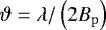 , where λ is the wavelength, and Bp is the projected baseline length. This is the usual convention in optical–IR interferometry.
Thus, we required that the azimuth difference between target and calibrator be <30°, and the airmass difference be <0.2.
The pipeline recipes are explained in detail in the MATISSE pipeline user manual, available at ftp://ftp.eso.org/pub/ dfs/pipelines/instruments/matisse/matisse-pipeline-manual-1.5.1.pdf
The non-default data reduction options were compensate = “pb,rb,nl,if,bp,od” in L-band; and corrFlux=TRUE, useOpdMod= TRUE, spectralBinning=7 in N-band.
The flux density values are expressed in unit frequency (ν), in units of Jy.
We did not determine a global uncertainty limit for the N-band closure phase because we do not use these data in the modeling.
Our data products are available in OIFITS format at the Optical interferometry DataBase (OiDB) at the Jean-Marie Mariotti Center (http://oidb.jmmc.fr).
Older K-band observations by VLTI/AMBER show closure phases in the range of − 60°⋯ + 40°, although with very large (~30°) uncertainties (Setterholm et al. 2018).
The fact that no extended component is needed in our model may suggest that the physical origin of the halo emission seen at shorter wavelengths in many Herbig stars is the scattering of the stellar light.
In the disk of HD 163296, the near side of the rim is located towards NE. This is supported by the velocity measurements of the jet and associated Herbig-Haro objects (Devine et al. 2000), and by the velocity mapping of the molecular gas emission (Teague et al. 2019).
The number of non-chopped exposures is 4N, where N is the number of exposure cycles.
All Tables
List of the best-fit parameters, half-light radii, and χ2-values in our L-band modeling.
List of the fitted and fixed parameters in our N-band modeling with the 2D Gaussian model.
List of the best-fit parameters, half-light radii, and χ2-values in the Gaussian L-band modeling.
All Figures
|
Fig. 1 uv-coverage of our observations. Blue crosses represent the data from 2019 March and May, orange crosses represent the data from 2019 June. |
| In the text | |
|
Fig. 2 Final L-band calibrated data products from the 2019 March (dashed lines) and May (solid lines) observations: spectrally resolved absolute visibilities (top), and closure phases (bottom). Error bars are indicated at a few random locations. |
| In the text | |
|
Fig. 3 Final N-band calibrated data products from the 2019 March observation (solid lines): correlated spectra (top), and closure phases (bottom). Error bars are indicated at a few random locations. For comparison, we plot the total spectrum on the top panel (dash-dot black line) measured with the TIMMI2 instrument (van Boekel et al. 2005b). |
| In the text | |
|
Fig. 4 Results of our model fitting for the L-band data with the asymmetric ring model: fits to visibilities against the deprojected baseline length in which the effect of the object inclination is removed (left), fits to closure phases (middle), and the best-fit model image at 3.2 μm (right). Baseline lengths are expressed in spatial frequency units. Data points are indicated by circles, model values by crosses. Left panel: symbols are color coded for the baseline position angle. The blue shaded area on the left panel represents the range of model visibility functions taken at different baseline position angles, at 3.2 μm wavelength. |
| In the text | |
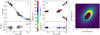 |
Fig. 5 Same as Fig. 4, but with the flat disk model. |
| In the text | |
|
Fig. 6 Gas surface density at the inner edge of a disk obtained with numerical simulation. The asymmetry in density is due to a vortex formed by the Rossby wave instability. |
| In the text | |
|
Fig. 7 Characteristic size of the emitting region as function of wavelength. The red points are derived from our MATISSE data. The 1.6 and 2.2 μm points come from PIONIER (Lazareff et al. 2017; Kluska et al. 2020) and GRAVITY (GRAVITY Collaboration 2019) observations, respectively. Black crosses represent our new fits to MIDI data published by Varga et al. (2018). The solid line is from the DIANA radiative transfer model of HD 163296 (Woitke et al. 2019). The dashed line corresponds to our flat diskmodel. |
| In the text | |
|
Fig. A.1 Flow chart of our data processing workflow. V indicates visibility, CP indicates closure phase, and Fcorr indicates correlated flux. |
| In the text | |
|
Fig. B.1 L-band transfer function during the night from 2019-03-22 to 2019-03-23. Gray shading indicates the observation time of HD 163296.The gray lines, one for each BCD configuration, are cubic polynomial fits to the points. In the captions, σ is the relative standard deviation of the transfer function values. |
| In the text | |
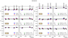 |
Fig. B.2 Same as Fig. B.1, but for the night from 2019-05-05 to 2019-05-06. |
| In the text | |
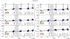 |
Fig. B.3 Same as Fig. B.1, but for the night from 2019-06-25 to 2019-06-26. |
| In the text | |
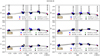 |
Fig. B.4 Same as Fig. B.1, but for the night from 2019-06-28 to 2019-06-29. |
| In the text | |
|
Fig. C.1 Posterior distributions for the smoothed ring model in L-band from our MCMC sampling. Blue lines represent the best-fit values. |
| In the text | |
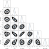 |
Fig. C.2 Same as Fig. C.1, but for the flat disk temperature gradient model. |
| In the text | |
|
Fig. D.1 Same as Fig. 4, but with the Gaussian plus point source model. Panel c: indicate the locations of the central star (star symbol) and of the additional point source (circle). |
| In the text | |
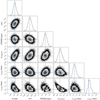 |
Fig. D.2 Same as Fig. C.1, but for the Gaussian plus additional point source model. |
| In the text | |
Current usage metrics show cumulative count of Article Views (full-text article views including HTML views, PDF and ePub downloads, according to the available data) and Abstracts Views on Vision4Press platform.
Data correspond to usage on the plateform after 2015. The current usage metrics is available 48-96 hours after online publication and is updated daily on week days.
Initial download of the metrics may take a while.