| Issue |
A&A
Volume 699, July 2025
|
|
|---|---|---|
| Article Number | A112 | |
| Number of page(s) | 24 | |
| Section | Cosmology (including clusters of galaxies) | |
| DOI | https://doi.org/10.1051/0004-6361/202453299 | |
| Published online | 04 July 2025 | |
Understanding entropy in massive halos: The role of baryon decoupling
1
INAF – IASF Milano, Via A. Corti 12, I-20133 Milano, Italy
2
Dipartimento di Scienza e Alta Tecnologia, Università dell’Insubria, Via Valleggio 11, I-22100 Como, Italy
3
DIFA – Università di Bologna, Via Gobetti 93/2, I-40129 Bologna, Italy
4
INAF – Osservatorio Astronomico di Brera, Via E. Bianchi 46, I-23807 Merate (LC), Italy
5
Department of Physics, Informatics and Mathematics, University of Modena and Reggio Emilia, I-41125 Modena, Italy
6
Dipartimento di Fisica, Università degli Studi di Milano, Via G. Celoria 16, I-20133 Milano, Italy
7
INAF – Osservatorio Astrofisico di Arcetri, Largo E. Fermi, I-50122 Firenze, Italy
⋆ Corresponding author: silvano.molendi@inaf.it
Received:
4
December
2024
Accepted:
13
February
2025
Aims. The goal of the work presented in this paper is to use observed entropy profiles to infer constraints on the accretion process in massive halos.
Methods. We compare entropy profiles from various observational samples with those generated by an updated version of the semi-analytical models developed in the early 2000s, that have been modified to reflect recent advancements in our understanding of large-structure formation.
Results. Our model reproduces the growing departure from self-similarity observed in data when moving inward in individual profiles and down in mass across different profiles. These deviations stem from a phase of extremely low gas content centered around 1013 M⊙. According to our model, halos at this mass scale are missing between 50% and 90% of their baryons, corresponding to a gas fraction ranging between 2% and 8%.
Conclusions. Baryon decoupling, the mechanism at the heart of our model, proves effective in explaining much of the behavior we sought to understand.
Key words: galaxies: abundances / galaxies: clusters: general / galaxies: clusters: intracluster medium / intergalactic medium
© The Authors 2025
 Open Access article, published by EDP Sciences, under the terms of the Creative Commons Attribution License (https://creativecommons.org/licenses/by/4.0), which permits unrestricted use, distribution, and reproduction in any medium, provided the original work is properly cited.
This article is published in open access under the Subscribe to Open model. Subscribe to A&A to support open access publication.
1. Introduction
It has long been understood that the high entropy of gas in massive halos (Mh ≳ 1013 M⊙) is a direct consequence of the virialization process. In simple terms, gas falls onto the halo, and around the virial radius, it converts its kinetic energy into thermal energy by impacting other gas, that is at rest in the potential well of the system. Since the sound speed in the infalling gas is much smaller than the infall velocity, the impact generates a shock that raises the entropy of the gas. In stark contrast, once inside the halo, the processes operating on the gas are largely adiabatic, and both conduction and mixing are highly suppressed (see Molendi et al. 2023, and references therein), leaving the entropy unaltered. Thus, by measuring the entropy of the gas in massive halos, one can acquire valuable information on shock heating at the virial radius and, ultimately, on the accretion process.
The goal of the work presented in this paper is to use observed entropy profiles to infer constraints on the accretion process. In pursuing this objective, we adopted a semi-analytical approach. As discussed by a few authors two decades ago (Tozzi & Norman 2001; Voit et al. 2003; Voit 2005), the process by which entropy is generated is a simple one: the bulk of the entropy is generated at the virial shock. Early semi-analytical work (Tozzi & Norman 2001; Voit et al. 2003; Voit 2005) met with some success, as the predicted slopes broadly aligned with observations of massive clusters. However, with the advent of more precise measurements (see Pratt et al. 2006, 2010), it became clear that even beyond the core region, where processes such as radiative cooling and heating from the active galactic nucleus (AGN) heavily influence gas thermodynamics, these simple models fall short of explaining critical features. Specifically, lower mass systems exhibited entropy profiles that, when rescaled self-similarly, were offset relative to those of more massive systems. This discrepancy indicates that the self-similar scaling inherent in the models fails to capture some essential physical processes. To address these limitations, semi-analytical studies were quickly supplemented (Borgani et al. 2005; Voit et al. 2005) and later largely supplanted by simulation-based approaches (see Altamura et al. 2023, and references therein). While simulations have successfully overcome several obvious shortcomings of earlier models, they introduce their own set of challenges, such as computational complexity, resolution limitations, and uncertainties in modeling sub-grid physics such as feedback and cooling processes. Here, we aim to determine whether and to what extent an updated version of the semi-analytical models from the early 2000s, incorporating significant advancements in the understanding of large-structure formation, can account for the extensive observational evidence gathered over the past two decades.
As mentioned earlier, reproducing observed entropy profiles represents a step toward a broader goal: gaining deeper insights into the accretion process. This focus distinguishes our approach from much of the simulation work in recent years (e.g., Barnes et al. 2017; Altamura et al. 2023; Braspenning et al. 2024). Simulations typically employ detailed descriptions of numerous processes governing the formation and evolution of large-scale structures in the Universe and are aiming at predicting a wide array of baryonic properties across different states and scales, with entropy profiles being just one among many. The two approaches are complementary: findings based on simulations offer a framework for conducting targeted studies of specific aspects of structure formation, while semi-analytical efforts, such as the one presented in this paper, provide insights into particular processes that can subsequently be incorporated into simulations.
The paper is organized as follows. Sect. 2 reviews the process of entropy generation as outlined in the semi-analytical studies of the early 2000s. In Sect. 3 we derive radial entropy profiles by combining the entropy-halo mass relation obtained in Sect. 2 with the radial mass distribution. We also show that these profiles align reasonably well with observations at large radii, though they fall significantly below observed values at smaller radii. In Sect. 4, we illustrate that incorporating pre-heating into the entropy generation process reduces the discrepancy between the model and the observed data, but it does not resolve it. In Sect. 5, we modify the self-similar accretion model by decoupling the accretion of baryons from that of dark matter. We demonstrate that the ensuing break in self-similarity can be recovered in part by rescaling entropy by the gas fraction. In Sect. 6, we compare entropy and density profiles derived assuming baryon decoupling with observed profiles from three different samples of galaxy clusters and one sample of X-ray bright galaxy groups, overall finding good agreement. We also argue that the difference between observed profiles of other, less X-ray bright groups and those predicted from our model can be resolved by invoking heating from the central AGN. In Sect. 7, we compare predictions from our model with those from other theoretical work. In Sects. 8 and 9 we respectively discuss and summarize our findings.
Throughout the paper we assume a Λ cold dark matter cosmology with H0 = 70 km s−1 Mpc−1, ΩM = 0.3 and ΩΛ = 0.7 Furthermore, we define RΔ as the radius inside which the cluster mass density is Δ times the critical density of the Universe, and MΔ is the halo mass within RΔ.
2. Entropy generation
We start by reviewing the spherical accretion model discussed by several authors (e.g., Tozzi & Norman 2001; Voit 2005) two decades ago. In simple terms, the accretion of gas in massive halos can be divided into three phases: a first phase where gas falls onto the halo, a second where it is shock heated and a third where it settles into near hydrostatic equilibrium within the halo. An important point is that the processes occurring in the first and third phase are assumed to be adiabatic and therefore leave the entropy of the gas unaltered. The variation in entropy occurs only in the second phase, this crucial aspect is nicely represented in Fig. 2 of Tozzi & Norman (2001). Furthermore, the whole process is assumed to be radially symmetric and can be described in terms of smooth accretion of spherical shells that are shocked at a single radius, namely the virial radius.
2.1. Baseline model
In the simplest case, the gas starts off cold and acquires all its entropy by going through a shock at the virial radius. Under these conditions the equations describing the shock can be reduced to a set of four, (see Eqs. 67–70 in Voit 2005). We re-propose them here.
The mass flow through the accretion radius is
where  is the gas accretion rate, Rv is the virial radius which coincides with the shock radius, ρg, u is the upstream gas density and vv is the gas velocity at the virial radius.
The velocity of the accreted gas is described with

where Mh is the halo mass. Eq. (2) is derived by equating the kinetic energy at the virial radius to the variation in potential energy between the turn-around radius, where velocity is zero, and the accretion radius, under the assumption the turn around radius is, Rta = 2 Rv.
The equation for energy conservation is
where kb is the Boltzmann constant, μ is the mean molecular mass of the gas and mp is the proton mass. Eq. (3) describes the conversion of the upstream kinetic energy (right hand side) into downstream thermal energy (left hand side).
For gas compression the equation is

where ρg, d and ρg, u are respectively the gas density downstream and upstream of the shock. Eq. (4) relates the upstream to the downstream density of the gas under the assumption of high Mach number, in which case the downstream density is 4 times the upstream one. We note that this set of equations provides an approximate description of the process valid for strong shocks. For instance, it does not account for the compression and adiabatic heating undergone by the infalling gas before being shocked (see Tozzi & Norman 2001, for details). We nonetheless work within the framework provided by Eqs. (1)–(4) and evaluate the impact of the approximations at the appropriate time.
From Eqs. (1), (2) and (4) one can rewrite the downstream density as a function of halo mass, gas accretion rate and accretion radius:
Similarly, from Eqs. (2) and (3), the gas temperature may be expressed as a function of halo mass and accretion radius:
Making use of Eqs. (5) and (6), one can write the entropy1, which following Balogh et al. (1999), we define as
in the form
Assuming that the gas fraction of the shells undergoing accretion is constant and equal to the cosmic baryon value, we may write

where fb is the cosmic baryon fraction and  is the matter accretion rate on the halo. Thus, Eq. (8) can be rewritten in the form
2.2. Entropy versus mass relation
Within the framework we have explored, the relationship between entropy and halo mass is described by Eq. (10). To estimate the halo mass, Mh, and its growth rate,  , we make use of the analytical model described in Salcido et al. (2020) (see their Eq. 12 and Fig. 3). In Fig. 1 we show the case of three halos of 1013 M⊙, 1014 M⊙, and 1015 M⊙, respectively, at z = 0. The entropy has been rescaled by dividing by
  , where Mh, o ≡ Mh(z = 0).
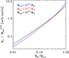 |
Fig. 1. Scaled entropy versus halo mass relation for three halos of 1013 M⊙, 1014 M⊙, and 1015 M⊙ at z = 0, respectively. |
There are two key points to highlight. First, the growth of entropy with halo mass for the three systems is similar. This arises from the weak dependency of the specific accretion rate,  , on Mh, o, as illustrated in Fig. 2. Second, entropy increases more rapidly with decreasing Mh, o. This behavior can again be attributed to the relationship between entropy and the specific accretion rate. As shown in Fig. 2, the specific accretion rate decreases more significantly with decreasing Mh, o.
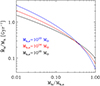 |
Fig. 2. Specific accretion rate versus halo mass relation for three halos of 1013 M⊙, 1014 M⊙, and 1015 M⊙ at z = 0, respectively. |
An interesting way of characterizing the entropy versus halo mass relationship is through the logarithmic slope dlnKv/dlnMh (see Voit et al. 2003). It can be shown, see Appendix A for a derivation, that the following relation holds:
where α ≡ dlnMh/dlnt.
The logarithmic slope dlnKv/dlnMh is reported in Fig. 3 for three halos of 1013 M⊙, 1014 M⊙ and 1015 M⊙ at z = 0 respectively. As pointed out in Voit et al. (2003), the increase in slope at large values of Mh/Mh, o is related to a decrease in accretion rate, see Fig. 2.
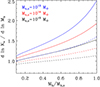 |
Fig. 3. Logarithmic slope, dlnKv/dlnMh, versus halo mass relation for three halos of 1013 M⊙, 1014 M⊙, and 1015 M⊙ at z = 0, respectively, as estimated from Eq. (11). Dashed lines were computed neglecting the dlnα/dlnMh term. |
3. Radial entropy profiles
In this section we derive radial entropy profiles from the model presented in Sect. 2. We do this in three steps. First we make use of Eq. (10) that relates entropy to halo mass, then we assume a radial mass distribution, finally we combine the two to derive the radial entropy profile.
As we shall see later, in the last step we consider two distinct approaches to derive entropy profiles. The first is a straightforward combination of the functional forms: K(R) = Kv(Mh(R))2, the second imposes that gas within the halo follow hydrostatic equilibrium.
3.1. Mass versus radius relation
Several relations have been proposed in the literature to describe the distribution of mass within a halo (e.g., Ettori et al. 2019, and references therein), we assume one of the mostly commonly used, the Navarro, Frank, and White (NFW) profile (Navarro et al. 1997). We write the mass within a radius R as:
![$$ \begin{aligned} M_{\rm h}({ < }R) = 4 \pi \rho _o R_{\rm s}^3 \left[\ln (1+x) - {x \over 1+x}\right], \end{aligned} $$](/articles/aa/full_html/2025/07/aa53299-24/aa53299-24-eq17.gif)
where ρo is a reference density, x = R/Rs, and Rs is the scale radius. Furthermore, we fix the shape of the profile by assuming that c200, defined as: c200 ≡ R200/Rs, assumes the value c200 = 4. We point out that variation of c200 within reasonable limits (e.g., Ettori et al. 2019) do not change results presented later. Furthermore, for a ΛCDM Universe, with ΩM = 0.3 and ΩΛ = 0.7, the virial overdensity at z = 0 is Δv(z = 0)∼100 (see Eq. 44 in Voit 2005) and the virial radius is: Rv ∼ 1.25 R200. Thus, the concentration computed using the virial radius, which is defined as: cv ≡ Rv/Rs, turns out to be: cv ∼ 5.
3.2. Analytical derivation of the slope of the entropy profile
Interestingly, the logarithmic slope of the NFW mass profile can be expressed as
By writing:
and substituting Eqs. (11) and (13) into Eq. (14), we obtained
This expression allows us to perform a direct computation of the logarithmic slope of the radial entropy profile, which we report in Fig. 4, for three halos of 1013 M⊙, 1014 M⊙ and 1015 M⊙ at z = 0 respectively.
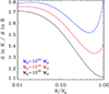 |
Fig. 4. Logarithmic slope of the radial entropy profile for three halos of 1013 M⊙, 1014 M⊙, and 1015 M⊙ at z = 0, respectively, as estimated from Eq. (15). The radial coordinate has been normalized to the virial radius. |
As can be appreciated, the slopes of the three entropy profiles differ considerably. Since the term in Eq. (15) coming from Eq. (13) does not depend on mass (the NFW profile is self-similar) the difference between the three curves is entirely due to the term coming from Eq. (11) and more specifically to α and dlnα/dlnMh.
3.3. Radial entropy profiles
As discussed at the beginning of this section, we compute entropy and other thermodynamic profiles in two different ways. In the first, we perform a straightforward combination of the functional forms: K(R) = Kv(Mh(r)), in the second we impose hydrostatic equilibrium on the shocked gas. We note that, in the first case, the gas fraction averaged within the shock radius remains unchanged with respect to the one we impose on the infalling shells. In the second, gas is allowed to reorganize itself. As in Tozzi & Norman (2001), we solve for hydrostatic equilibrium from the outside. We take the values of thermodynamic values at the shock radius as boundary conditions and numerically solve a set of three equations: the hydrostatic equilibrium equation, the gas mass conservation equation and the entropy conservation equation. This allows us to derive radial profiles for all thermodynamic variables. A detailed description of the procedure is provided in Appendix B.
In Fig. 5 we plot radial entropy profiles for three different halo masses: 1013 M⊙ (left panel), 1014 M⊙ (central panel) and 1015 M⊙ (right panel). We note that the radius has been normalized to the shock (virial) radius and the entropy has been divided by the entropy at the virial radius, Kv. As we may surmise from the figure, the two solutions, shown respectively in blue and black, do not differ much from one another, both become steeper as we move inward as highlighted by a comparison with a reference power-law profile (red line). Numerical computation of the dlnK/dlnr curves, obtained from the solution derived through a straightforward combination of functional forms, shows them to be in excellent agreement with the ones computed analytically (see Eq. 15) and shown in Fig. 4.
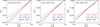 |
Fig. 5. Predicted entropy profile for a halo mass of 1013 M⊙ (left panel), 1014 M⊙ (central panel), and 1015 M⊙ (right panel). The radius has been normalized to the shock (virial) radius. All profiles are normalized at the shock radius. In red we plot a reference powerlaw with slope 1.2, in blue the profile derived from a combination of the functional forms: K(R) = Kv(Mh(R)) and in black the one derived by solving the hydrostatic equilibrium equation. |
It is worth noting that, for the cluster mass range, 1014 M⊙ − 1015 M⊙, these results, are consistent with those derived from non-radiative cosmological simulations performed using both Lagrangian smoothed particle hydrodynamics (SPH: see Borgani et al. 2002; Rasia et al. 2004) and Eulerian adaptive mesh refinement codes (see Voit et al. 2005). This tells us something quite important: a simple one dimensional model, based on mass and energy conversion arguments, provides a description of the entropy generation process which is, at least to first order, comparable to that which can be achieved through a much more detailed and computationally intensive analysis.
3.4. A first comparison with observations
A detailed comparison with observations is presented in Sect. 6. Here, we wish to ascertain if the simple model outlined above provides estimates that are at least broadly consistent with available data. In Fig. 6 we compare the entropy profiles derived imposing hydrostatic equilibrium, and already presented in Fig. 5, with the median profile derived from the REXCESS sample of galaxy clusters (Pratt et al. 2010). To ease comparison with observational data, entropy has been rescaled by K500, which is defined as in Pratt et al. (2010), see their Eq. (3), and radius by R500. At large radii, R ∼ R500, the predicted entropy is broadly consistent with the measured one, however, as we move inwards, the behavior of measured and predicted profiles diverge, the latter featuring a much steeper decline than the former. In more physical terms, the entropy generated purely from gravitational shocks is consistent with the observed one in the outskirts but severely under-predicts it at smaller radii. Both agreement and disagreement are rich in significance. The agreement suggests that, to first order, a description of the virialization process that is as crude as the one we presented, can reproduce observed data. This implies that the entropy generation process is probably not too dissimilar from a total conversion of kinetic energy into thermal energy at a single shock radius3. It is worth pointing out that, although highly desirable, such an outcome is by no means guaranteed. Indeed, in light of the limited understanding of the physics of the accreted gas compounded by the dearth of observational data, the entropy generation process could just as easily have taken very different forms. Just as an example, Vazza et al. (2009) present simulations of the accretion process on massive halos in which thermalization occurs over an extremely broad radial range, with kinetic energy exceeding thermal energy for radii larger than 0.75 Rv and remaining as high as 30% of the thermal energy down to ∼0.3 Rv.
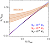 |
Fig. 6. Predicted entropy profiles for a halo mass of 1013 M⊙ (blue), 1014 M⊙ (red) and 1015 M⊙ (black) respectively, compared with the observed mean entropy profile and intrinsic scatter (orange shaded region) from the REXCESS sample of galaxy clusters, (Pratt et al. 2010), which features a median mass of M500 ∼ 2.5 × 10¹⁴ M⊙. To ease comparison with observational data, the predicted entropy has been rescaled by K500 and radius by R500. |
Regarding the disagreement at smaller radii, it has been known since the time scaling relations were first established (Kaiser 1986, 1991), that non-gravitational forms of heating, including AGN feeding/feedback (e.g., Gaspari et al. 2020, for a review), may provide an important contribution. Some two decades ago, several authors (e.g., Tozzi & Norman 2001; McCarthy et al. 2004; Voit 2005) developed models in which the self-similar shape of entropy profiles was at least partially modified by assuming that the infalling gas was pre-heated to a fraction of the virial temperature. In the following section we revisit pre-heating.
4. Pre-heating
Pre-heating is the process by which gas is heated prior to being accreted. As pointed out in Tozzi & Norman (2001), the pre-heated gas contracts in an approximately adiabatic fashion as long as its temperature is larger than the virial temperature of the halo onto which it is falling. Under such conditions no virial shock forms and the entropy of the accreted gas is essentially that of the pre-heated gas. As soon as the virial temperature grows beyond the temperature of the infalling pre-heated gas, an accretion shock forms.
As discussed in a seminal paper (Kaiser 1991), pre-heating is likely associated to the galaxy formation process. Pre-heating introduces a flat region in the radial entropy profile. The gas residing in such an iso-entropic region has been accreted without being shocked and retains the entropy it had prior to its accretion. As shown in Voit et al. (2003), the entropy of the gas including the effects of preheating KWP, can be expressed reasonably well as the sum of the entropy of the gas without pre-heating, Kv, and the entropy of the preheated gas, K* multiplied by a correction factor:

A crucial point is the estimate of the pre-heating entropy. Several authors (e.g., Tozzi & Norman 2001; McCarthy et al. 2002; Ponman et al. 2003; Voit et al. 2003) have proposed values in the range 1 − 5 × 1033 erg cm2 g−5/3. These estimates were arrived at by comparing observed scaling relations or entropy profiles with models including pre-heating. In Sect. 5 we discuss a different approach to estimating K*.
In Fig. 7 we show entropy profiles for a halo mass of 1013 M⊙, 1014 M⊙ and 1015 M⊙ respectively. The entropy of the pre-heated gas is set to the value generated through gravitational processes at the virial radius of a 1013 M⊙ halo: K* = Kv(Mh = 1013 M⊙)∼3.5 × 1033 erg cm2 g−5/3, for all three halo masses (for a justification of this choice see Tozzi & Norman 2001, and Sect. 5.6). As can be observed, the effect of pre-heating strongly depends on the halo mass. For the 1013 M⊙ system, it provides the dominant contribution at all radii. At the opposite mass end, 1015 M⊙, its effects can be appreciated only for R < 0.1 R500. In somewhat different terms, we can say that pre-heating produces a departure from self-similarity that is strongly halo mass dependent.
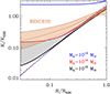 |
Fig. 7. Predicted entropy profiles for a halo mass of 1013 M⊙ (blue), 1014 M⊙ (red), and 1015 M⊙ (black). Dashed lines show entropy from gravitational processes only, solid lines include the effects of pre-heating. The mean entropy profile and intrinsic scatter from the REXCESS sample of galaxy clusters, (Pratt et al. 2010), which features a median mass of M500 ∼ 2.5 × 10¹⁴ M⊙, is reported as an orange shaded region. The region between the 1014 M⊙ and 1015 M⊙ profiles is shown as a gray shaded region. |
As far as the comparison with observations is concerned, pre-heating does significantly reduce the differences between modeled and observed profiles but it does not allow for agreement between the two. With the pre-heating modification to the model, predicted entropy profiles of clusters fall between the thick red (1014 M⊙) and blue (1015 M⊙) curves, observed ones do not. In particular, in observed clusters, the excess with respect to the gravity only model (dashed lines in Fig. 7) is present up to intermediate radii R ∼ 0.5 R500, while in modeled systems, with halo masses Mh ≳ 1014 M⊙, it is found only at smaller radii.
It is worth pointing out that cooling has not been introduced in the gravity only or the pre-heating modified model, this limits the applicability of the models to regions beyond the core, R ≳ 0.1 R500, where the cooling time of the gas is sufficiently long, we return to this point in Sect. 6.2, where we perform a more detailed comparison with observations.
5. Baryon decoupling
The pre-heating model described in Sect. 4 and in the literature (see Voit 2005, and references therein) manifestly fails to reproduce the shape of entropy profiles in clusters.
In this section, we investigate a different description of feedback processes in the hope that it will lead to a better agreement with observations. In doing so, we take stock of the considerable advances that have taken place over the past two decades.
5.1. Advancements
One of the most important things we have learned is that the halo mass range between a few 1012 M⊙ to 1013 M⊙ plays a critical role in the evolution of baryons. This is where star formation shuts down (e.g., Leauthaud et al. 2012; Coupon et al. 2012, 2015; Behroozi et al. 2013, 2019; Moster et al. 2013; Cowley et al. 2018; Legrand et al. 2019; Girelli et al. 2020; Shuntov et al. 2022). Equally important is the fact that the position of the star formation peak is largely insensitive to cosmic time, for z ≲ 4 as shown in (Behroozi et al. 2013, 2019; Legrand et al. 2019). The cold baryon reservoir from which stars form is suddenly and dramatically emptied, quite possibly through feedback from the central AGN that heats up and disperses the cold gas. The same process likely leads to a substantial reduction in the accretion on the central black hole. However, the significantly different scales on which star formation and AGN feeding operate likely lead to a delay between the shutting down of the latter with respect to the former. It is worth pointing out that the observed correlation between stellar mass and Black Hole mass, (see Zhang et al. 2024a, and references therein) as well as the one between hot halo properties and super-massive black hole (SMBH) mass (Gaspari et al. 2019) are consistent with this scenario.
Relatively little is known of the heated gas, it is most likely in a hot phase either within the halo, in which case it is referred to as the hot phase of the circum galactic medium (see Tumlinson et al. 2017, and references therein) or outside it, in which case it takes the name of warm hot intergalactic medium (see Nicastro et al. 2022, and references therein). Another important piece of the puzzle that has emerged over the past decade is that the gas fraction, fg, in massive halos, correlates with halo mass (see Eckert et al. 2021, and references therein), with lower mass systems featuring a significantly smaller baryon fraction than more massive ones. Putting the two pieces together, we may surmise that somewhere around ∼1013 M⊙, the feedback events responsible for shutting down the accretion also lead to a significant evacuation of baryons from the halo. The substantial scatter in gas fraction observed in groups most likely reflects the stochastic nature of the process. Feedback processes operate on a wide range of halo masses, and to avoid confusion, we refer to feedback on ∼1013 M⊙ halos as early-time feedback, while those operating on more massive halos are described as late-time feedback. Within this framework, the increase in gas fraction observed for halo masses larger than ∼1013 M⊙, corresponds to a phase of slow re-accretion of gas previously ejected by less massive halos. It is worthwhile reminding our readers that we do have indirect evidence of the accretion of pre-enriched hot gas in massive halos through metals (see Molendi et al. 2024).
5.2. A simple prescription
Having taken stock of what has been learned over the past two decades, we modify the self-similar accretion model described in Sects. 2 and 3 by decoupling the accretion of baryons from that of dark matter. Baryon decoupling provides a very simple modification, one might argue the simplest possible modification, to satisfy the constraints described in Sect. 5.1. In this section we develop a model based on baryon decoupling and see how far it takes us in interpreting the thermodynamic properties of massive accretors. Before proceeding with the actual modification it is instructive to perform a little bit of deductive reasoning to see how differences between measured and predicted entropy might be explained by baryon decoupling.
Our approach is somewhat analogous to methods used by geologists when studying rock stratification. Similarly, in massive halos, gas stratifies by entropy, with gas accreted earlier positioned closer to the center, while gas accreted later resides in the outer regions. Comparison with observations, see Figs. 6 and 7, shows that the entropy generated when the halo was a fraction of its current mass is higher than expected. From Eq. (7) we see that a higher entropy might result from a lower density. A lower density likely follows from a lower gas accretion rate with respect to the one assumed in Eq. (9), namely:

or in other words, from baryon decoupling.
At least qualitatively, baryon decoupling goes in the direction required to reconcile the self-similar model with observations. A more quantitative assessment requires the definition of a gas fraction versus halo mass relation. To this end, we assume decoupling to take place at a specific halo mass, roughly 1013 M⊙. At much smaller and larger masses we assume baryon accretion to be coupled to dark matter accretion. A simple way to describe this process mathematically is through the formula:
![$$ \begin{aligned} \log (f_{\mathrm{g}}) = \log (f_{\mathrm{b}}) + {l_{\rm n} \, {\exp \left[-{1\over 2}\left({\log M_{\rm h} - l_{\rm m} \over l_{\sigma }}\right)^2\right]}}, \end{aligned} $$](/articles/aa/full_html/2025/07/aa53299-24/aa53299-24-eq23.gif)
where log(fg) is the base ten logarithm of fg, log(fb) is the base ten logarithm of fb, and 10lm M⊙ is the halo mass at which baryon decoupling is strongest (i.e., where the deviation of the gas fraction, fg, from the cosmic baryon fraction reaches its maximum). The second parameter quantifies the decoupling: 10ln is the ratio of the gas fraction over the cosmic baryon fraction at Mh = 10lm M⊙, and finally lσ determines the halo mass range over which the gas fraction is decoupled from the cosmic baryon fraction.
In Fig. 8 we show, as a red solid line, a realization of the gas fraction versus halo mass relation for a representative choice of parameters. Additionally, the figure shows the gas mass versus halo mass relation as a black solid line, highlighting another key relation. We note how, despite the reduction in gas fraction with increasing halo mass for Mh < 10lm M⊙, the gas mass always increases with halo mass.
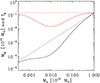 |
Fig. 8. Gas fraction, fg, shown in red and gas mass, Mg, shown in black, as a function of halo mass. The dashed lines show the case where fg = fb and Mg = fbMh at all halo masses. The solid lines show the case modeled by Eq. (18) with parameters chosen as follows: lm = 13, ln = −1, and lσ = 0.6. |
Our implementation of baryon decoupling provides a very simple modification of the gravitational entropy generation process. It identifies a critical mass at which baryon decoupling operates, 10lm M⊙, and allows for variations in the strength and the range over which the modification operates, respectively through the ln and lσ parameters. In the next subsection we develop a model based on baryon decoupling and see how far it takes us in interpreting the thermodynamic properties of massive accretors.
5.3. Entropy versus mass relation with decoupling
In this subsection we investigate the effects of baryon decoupling on the entropy versus halo mass relation. The first thing to note is that, since the gas fraction of the accreted shells is no longer constant, Eq. (10) is not valid and we have to fall back on Eq. (8). Furthermore, the  term, which in the case of fg = fb is simply
  , for a non-constant fg takes the form
Since the logarithmic derivative dlnfg/dlnMh is negative for Mh < 10lm M⊙ and positive for Mh > 10lm M⊙, the term in parenthesis on the right hand side of Eq. (19) reaches a minimum at Mh = 10lm M⊙. Multiplication by the  term shifts the minimum to somewhat lower halo masses. This is clearly seen in Fig. 9, where we plot
  as a function of halo mass for a halo of 1015 M⊙ at z = 0.
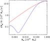 |
Fig. 9. Gas accretion rate versus halo mass relation for a halo of 1015 M⊙ at z = 0. The blue and red lines have been computed assuming fg follows respectively Eq. (18) and fg = fb. |
In more physical terms, baryon decoupling reduces the gas accretion rate with respect to the fg = fb case. Most importantly, it introduces a critical mass ∼1/4 10lm M⊙, below which the gas accretion rate decreases and above which it increases, with increasing halo mass. For halos that grow well beyond the critical mass, the accretion rate slowly converges to  , see Fig. 8. In other words, baryon decoupling does not halt accretion, it delays it.
As shown in Fig. 10, baryon decoupling induced deviations propagate from the gas accretion rate to the entropy. Comparison of the solid curves derived assuming fg follows Eq. (18) with dashed ones for which fg = fb, shows that baryon decoupling has a strong impact on the rescaled entropy versus halo mass relation. The reduction in accretion rate leads to an increase in entropy. As expected, the effect is largest for the least massive halos (3 ⋅ 1013 M⊙, 1014 M⊙ at z = 0), where the reduction in accretion rate is strongest. Another important point that is clearly observed in Fig. 10 is that baryon decoupling leads to a break in self-similarity; once again it is the less massive systems that deviate most. Finally, the change in slope observed for Mh/Mh, o ∼ 0.2, for the cases Mh, o = 3 ⋅ 1013 M⊙ and Mh, o = 1014 M⊙, is related to the minimum in  observed in Fig. 9.
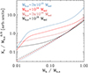 |
Fig. 10. Rescaled entropy versus halo mass relation for four halos of 3 ⋅ 1013 M⊙, 1014 M⊙, 3 ⋅ 1014 M⊙, and 1015 M⊙ at z = 0 respectively. Filled lines have been computed assuming fg follows Eq. (18), dashed ones assuming fg = fb. We note how baryon decoupling produces a break in self-similarity. The change in slope observed at small Mh/Mh, o values for the 3 ⋅ 1013 M⊙ and 1014 M⊙ at z = 0 halos is associated to the minimum in |

5.4. Gas fraction rescaling
With a little algebra Eq. 8 can be rewritten in the following fashion:
![$$ \begin{aligned} K_{\rm v} = {1 \over 3} \, (\pi G^2)^{2/3} \, \left({M_{\rm h} \over f_{\rm g}}\right)^{2/3} \left[{\dot{f}_{\rm g} \over f_{\rm g}} + {\dot{M}_{\rm h} \over M_{\rm h}}\right]^{-2/3}. \end{aligned} $$](/articles/aa/full_html/2025/07/aa53299-24/aa53299-24-eq32.gif)
This form highlights the similarity between the role played by Mh and fg. We recall that the self-similar scaling with respect to mass follows from the fact that  depends only weakly on mass, see Fig. 2. Something similar may happen with fg if
  is independent or at least weakly dependent on fg. Having identified a specific prescription for fg, see Eq. (18), we can verify to what extent fg scaling might work. In Fig. 11 we plot
  ,
,  and
and  as a function of halo mass for four halos of 3 ⋅ 1013 M⊙, 1014 M⊙, 3 ⋅ 1014 M⊙ and 1015 M⊙ at z = 0 respectively. The
  (dashed lines) are very similar to one another, this has already been shown in Fig. 2. It is this behavior that is responsible for self-similarity in the fg = fb case. The
  curves (dotted lines) show somewhat larger variations. However, since
  and
and  curves have opposite dependencies on halo mass, the
  (filled lines) show smaller variations on halo mass, with typical deviations from one another of less than ∼30% for Mh/Mh, o ≳ 0.3, suggesting that self-similarity can be recovered, at least in part, by normalizing on the gas fraction.
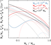 |
Fig. 11.
|


A comparison of Fig. 12 with Fig. 10 shows that rescaling by gas fraction does reduce variability between the different halos in a substantial way. This implies that the break in self-similarity associated to the decoupling between gas and dark matter accretion can be in large part recovered by rescaling the entropy by the gas fraction. However, we note that while all profiles are broadly similar at large fractional masses, as we move to smaller fractional masses, the lower mass systems deviate before the higher mass ones.
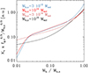 |
Fig. 12. Halo mass and gas fraction scaled entropy as a function of halo mass for four halos of 3 ⋅ 1013 M⊙, 1014 M⊙, 3 ⋅ 1014 M⊙, and 1015 M⊙ at z = 0, respectively. |
5.5. Entropy profiles with baryon decoupling
Following the procedure described in Sect. 3.3 we derive radial entropy profiles with baryon decoupling. As expected, we observe substantial deviations with respect to the self-similar profiles, see Fig. 13. More specifically, baryon decoupling augments entropy for all halo masses but it does so in different radial ranges for different halo masses. In broad terms we may say that, for Mh = 1013 M⊙ (blue line) the increase is concentrated at large radii, for Mh = 1014 M⊙ (red line) at intermediate radii and at small radii for Mh = 1015 M⊙ (black line). Intriguingly, the black solid line, which includes baryon decoupling, coincides with the dashed one which is derived assuming the baryon fraction of the accreting gas is constant, for radii larger than ∼0.4 R500. This is expected, as shown in Fig. 8, matter accreted on massive halos is close to having a cosmological baryon fraction. As pointed out in Sect. 5.3, baryon decoupling delays accretion, it does not stop it. An important consequence is that, in the outer regions of the most massive systems the entropy generation process is dominated by gravity, or in more explicit terms by the conversion of kinetic into thermal energy at the virial shock. We return to this important point in Sect. 6.1. The careful reader may note that also for the inner radii of low mass systems deviations from the gravitational heating model are modest. However, as discussed in Sect. 6.2, for R < 0.1 R500 radiative cooling, which is not included in our model, significantly modifies entropy profiles.
 |
Fig. 13. Radial entropy profiles derived by imposing hydrostatic equilibrium for a halo mass of 1013 M⊙ (blue), 1014 M⊙ (red) and 1015 M⊙ (black) respectively. The radius has been normalized to R500 and the entropy to K500. Filled lines have been computed with baryon decoupling, dashed ones without. |
To help readers keep track of the modifications we make to our model (see Sects. 5.6 and 6.1), in Fig. 14, we provide a model relationship tree.
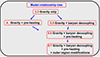 |
Fig. 14. Relationship tree connecting the models explored in this paper. The numbers in red at the left of the model name identify the section where the model is discussed. |
5.6. Entropy profiles with decoupling and preheating
Decoupling and pre-heating are not mutually exclusive, quite the contrary, early-time feedback processes that remove gas from shallow potential wells may also heat it. In this subsection we modify entropy profiles derived in Sect. 5.5 to include the effects of preheating.
As already discussed in Sect. 4, to provide a realistic entropy model, it is critical to estimate K*, the pre-heating contribution. To this end, we make use of what has been learned about feedback mechanisms over the past two decades. We proceed by estimating the temperature and the density of the preheated gas. Expulsion from low mass halos occurs when the temperature of the hotter phase of the gas exceeds the virial temperature. We set the temperature of the expelled gas to be: Texp = ΦTv(Mh = 0.3 − 1 × 10¹³ M⊙), where Φ is some yet to be determined factor. Regarding density, we start by noting that the mass of gas that is accreted onto the halo is much larger than what is involved in the star formation or central black hole feeding process. For halos of ∼0.3 − 1.0 × 10¹³ M⊙ roughly 1/7 of the baryon mass goes into stars (see Behroozi et al. 2019, and references therein). Assuming that roughly 1/3 of the gas that goes into stars is fed back (see discussion on the ro factor in Ghizzardi et al. 2021, and references therein), and that the contribution from the AGN feedback is negligible, as suggested by the fact that the black hole mass is less than ∼0.01 of the stellar mass (e.g., Reines & Volonteri 2015), we have that roughly 1/7 × 1/3 ∼ 5% of the baryons are involved in the feedback process. This implies that while the energy of the outflow will contribute significantly to that of the expelled gas, the mass contribution will be modest and for the present estimate negligible. Since the gas that requires the least energy to be expelled is the one that has just been accreted, we set the density of the expelled gas to that of the gas that has recently sustained a virial shock, ρexp ∼ ρv(Mh = 0.3 − 1 × 10¹³ M⊙). Coupling this with Texp = ΦTv(Mh = 0.3 − 1 × 10¹³ M⊙), which we derived earlier, we get Kexp = ΦKv(Mh = 0.3 − 1 × 10¹³ M⊙). Finally, we estimate that Φ cannot be much larger than a few, if it were ≳102/3 then the thermal energy of the gas would have been sufficient to inhibit accretion on objects that are 10 times more massive (clusters), which would in turn require clusters to have gas fractions comparable to those of less massive systems (groups). On the basis of this discussion, we include a preheating entropy of K* = Kv(Mh = M*)∼3.5 × 1033 erg cm2 g−5/3, where M* = 1013 M⊙. Since preheating only affects gas that is accreted on halos that are larger than the critical mass, M*, we implemented the preheating correction on entropy by multiplying K* by the factor exp(−M*/Mh), which goes respectively to one for Mh ≫ M* and to zero for Mh ≪ M*. This accounts for the fact that gas accreting on halos with mass comparable to M* is likely a mixture of cold and preheated, with cold becoming dominant as we move downwards in halo mass and preheated if we move in the opposite direction.
In Fig. 15 we show entropy profiles for a halo mass of 1013 M⊙ (blue), 1014 M⊙ (red) and 1015 M⊙ (black) respectively with baryon decoupling and pre-heating (filled lines), with baryon decoupling and no preheating (dashed lines), without either (dotted lines). As already shown in Fig. 13, baryon decoupling introduces significant modification to the entropy profiles. Conversely, including pre-heating on top of baryon decoupling introduces negligible modifications. This is fairly easy to understand, for small halo masses, Mh < 10lm M⊙, this is achieved by construction through the exponential cutoff term, exp(−M*/Mh) described above. For large halo masses, the accreted gas is all pre-heated, exp(−M*/Mh)∼1, but its contribution to entropy is negligible as in the preheating only model (see Fig. 6). We point out that changing the value of K* by a factor of a few results in very minor modifications, this justifies, in retrospect, the order of magnitude estimate we have made of this quantity.
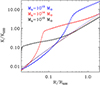 |
Fig. 15. Entropy profiles derived by imposing hydrostatic equilibrium for a halo mass of 1013 M⊙ (blue), 1014 M⊙ (red), and 1015 M⊙ (black), respectively. The radius has been normalized to R500 and the entropy to K500. Filled lines have been computed with baryon decoupling and pre-heating, dashed lines with baryon decoupling and no preheating, dotted lines without either. |
In summary, within massive halos, Mh ∼ 1015 M⊙, almost all the heat conferred to the gas is of gravitational nature. The role of feedback processes, while vital, requires relatively little energy, all that needs to be done is to take gas out of shallow potential wells and let gravity do the rest. The situation is radically different at the low mass end, Mh ∼ 1013 M⊙, here the energy of the expelled gas is sufficient to prevent, at least in part, its re-accretion.
6. Comparison with observations
This section is dedicated to a detailed comparison of the model we have developed with state of the art observations. We begin by focusing on the outer regions of massive clusters.
6.1. The outer regions of massive halos
On the base of the model described in the previous Section, it seems that the only place where entropy profiles depend only upon cosmological accretion is large radii in massive systems. Indeed, this is where both baryon decoupling and pre-heating play a negligible role, see Fig. 15. As shown in Figs. 6 and 7, the entropy predicted by the model is broadly consistent with the measured one, perhaps even a little on the high side: however, if one looks a little more in detail, one sees that the slopes are quite different, with observed profiles typically dlnK/dlnR ∼ 0.8 (Pratt et al. 2006; Ghirardini et al. 2019) and our model dlnK/dlnR ∼ 1.2.
As pointed out in Sect. 2, our modeling of the entropy generation at the accretion shock is relatively simple. Here we take a closer look at the process to gauge how a more realistic description might solve this issue. In very general terms there are two classes of corrections that may be applied. In the first, for some reason, the temperature and therefore the entropy of the shock heated gas does not increase with halo mass as  but at a slightly milder rate. In the second, the kinetic to thermal conversion occurs over a radial range, rather than just at one radius. In this case the entropy, rather than jumping from zero to the value in Eq. (10) at a specific radius, grows over a yet to be determined radial range.
6.1.1. From smooth to mixed accretion
In this subsection we discuss a minor modification to the smooth accretion framework that can have an effect on the entropy profiles in the outer regions of massive halos. Part of the gas undergoing shock heating is unbound, part is bound to infalling sub-halos. For the former part, all the kinetic energy associated to the infall is transformed into thermal energy, for the latter a fraction is required to strip the gas from the sub-halo. Thus, the mean temperature of the shocked gas will be lower than that estimated in the model described in Sect. 2, because part of the kinetic energy has been used up to free gas from sub-halos. As can be seen in Fig. 7 of Eckert et al. (2021), the fraction of gas bound to the halo, goes up with increasing halo mass. This implies that the mean temperature of the shock heated gas is progressively reduced as we go up in mass, with respect to what is predicted on the basis of Eq. (3). Through some relatively straightforward algebra we find that the ratio between the “mixed accretion” temperature, Tma and the temperature computed from Eq. (3), can be expressed as
where dn/dmh is the halo mass function, mh is a renormalized halo mass, Mh, o is the mass over which renormalization is carried out, Mmin is the minimum mass over which integration is extended, for which we adopt a value 5 × 10¹² M⊙. We note that integration is fairly insensitive to the specific value of Mmin as long as it is smaller than ∼1013 M⊙. For the gas fraction we adopt the expression presented in Eq. (18) with parameters used in Fig. 8. We note that the computation is insensitive to small variations on the parameters. A derivation of Eq. (21) is provided in Appendix C. Integration of Eq. (21) leads to variation of Tma(Mh)/T(Mh) of a few percent in the range 1013 M⊙ to 1015 M⊙. More specifically, when going from 1014 M⊙ to 1015 M⊙ we find a fractional temperature reduction of about 4%, see Fig. C.1, this is because more massive halos feature a larger fraction of bound gas. The net effect is a slightly lower growth of temperature and therefore entropy with increasing mass with respect to the case where evacuation of gas from sub-halos is not considered (see Sect. 5.6 and Fig. 14), leading in turn to a flattening of the entropy profile in the outer regions of massive clusters. The modification to the slope of the entropy profile, Δ(dlnK/dlnr)∼0.04, is however very modest and insufficient to reach agreement with observations. It is worth pointing out that ours is not the only approach that can be adopted to estimate a correction for mixed accretion. Furthermore, given the very gradual increase in the fraction of bound (or unbound) gas with increasing halo mass, the correction will likely be a modest one, regardless of the approach used.
6.1.2. From shock radius to shock region
The model described in Sect. 2 is based on the assumption that all the kinetic energy generated by gas motions within the gravitation field of the forming halo is converted into thermal energy through one shock occurring at one specific radius. There are some good reasons to think this cannot be the case.
As discussed in Sect. 5, a sizable fraction of the gas falling onto a massive cluster has been previously accreted and ejected by smaller halos. It will be characterized by a distribution in entropy and other thermodynamic variables. Within the infall region, conversion of kinetic into thermal energy through adiabatic compression will operate more effectively in hotter subregions (see Eqs. 3 and 3.5 respectively in Tozzi & Norman 2001; Pringle & King 2007), this will lead to velocity gradient with cooler subregions falling in more rapidly than hotter ones. As soon as velocity differences become of the order of the sound speed, shocks (i.e. non adiabatic thermalization) will kick in and further amplify velocity gradients, likely leading to a runaway process. Furthermore, the process by which collisionless shocks convert kinetic into thermal energy is far from being well understood (see Goodrich et al. 2023, and references therein). For all of these reasons, the radial extent of the virialization region is not easy to estimate, so we took a heuristic approach. We substituted the step function operating on entropy in the model described in Sect. 2 with a sigmoid that we implement through an hyperbolic tangent of the form
where Rv is the virial radius and s and h are two parameters that control the shape of the sigmoid. We note that 𝒮(R) goes to 1 for R ≪ Rv and 0 for R ≫ Rv. We also note that the modified entropy profile, K′(R), is related to the non-modified one through the relation: K′(R) = 𝒮(R) K(R).
We constrained the parameters characterizing the sigmoid through two measurements: (1) the entropy profiles in massive clusters, which, as pointed out above, have flatter slope than those predicted from our model; (2) the fraction of pressure in non-thermal form. The latter has been measured by several authors using different methods. Eckert et al. (2019), by comparing the hydrostatic mass with the total mass derived from the gas mass under the assumption that the gas fraction of massive clusters is close to the baryon fraction, find a non-thermal pressure support of ∼5% at R500 and ∼10% at R200. Wicker et al. (2023), applying a similar approach, come up with an hydrostatic mass bias factor4b of ∼20%. Dupourqué et al. (2024) analyzing surface brightness fluctuations on the CHEX-MATE sample, estimate a non-thermal pressure support of 9 ± 6% at R500. Lovisari et al. (2024), applying a similar approach to temperature maps from the CHEX-MATE sample, estimate a non-thermal pressure support of  . Finally, Muñoz-Echeverría et al. (2024) derive an hydrostatic to lensing mass bias factor of ∼25 ± 7%. Given the relatively large uncertainty in the non-thermal pressure contribution suggested by these measurements, we consider two scenarios: one assuming a larger contribution and the other a smaller one.
In Fig. 16 we plot the radial entropy profile for a halo of 1015 M⊙ at z = 0. The black filled line shows the profile in the case of a single shock at the virial radius, the blue filled line shows the case of a profile modified with a sigmoid to account for an extended shock region. Comparison with the dashed lines shows that the change introduced by the sigmoid flattens the slope to a value consistent with the one measured in observations.
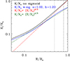 |
Fig. 16. Radial entropy profiles for a halo of 1015 M⊙ at z = 0. The black filled line shows the profile in the case of single shock at the virial radius. The blue filled line shows a profile modified with a sigmoid of the from reported in Eq. (22) and parameters shown in the figure. The vertical dotted and dashed lines mark the position of R500 and R200 respectively. The slope of the profiles can be gauged by comparison with the power laws plotted as dashed lines. |
The relationship between entropy modification and non-thermal pressure support depends on the details of the virialization process which, as pointed out above, are unknown. Assuming a simplified model in which the gas undergoes gradual heating within a given radial range accompanied by full instantaneous compression, n′(R) = n(R), we have that the relationship connecting the modified temperature with the unmodified one is: T′(R) = 𝒮(R) T(R). Similarly the modified pressure can be expressed as: p′(R) = 𝒮(R) p(R) and the fraction of pressure support of non-thermal origin is given by (p(R)−p′(R))/p(R) = 1 − 𝒮(R). Since 𝒮(R500)∼0.8 and 𝒮(R200)∼0.7, the modification shown in Fig. 16 implies a relatively high fractional non-thermal pressure support of 20% at R500 and 30% at R200, comparable to measurements such as Muñoz-Echeverría et al. (2024) and Wicker et al. (2023). We note also that if we relax the condition of full instantaneous compression and write: n′(R) = ℛ(R) n(R), with 0 < ℛ(R) < 1, the relation between modified and unmodified pressure becomes: p′(R) = 𝒮(R) ℛ(R)5/3 p(R) and the fraction of pressure support of non-thermal origin: 1 − 𝒮(R) ℛ(R)5/3, leading to an even larger non-thermal pressure support.
In Fig. 17 we show that by applying modifications that satisfy tighter constraints on the non-thermal pressure, roughly 5% at R500 and 10% at R200, changes in the entropy profile are more modest, with the slope of the modified entropy profile in the outskirts reaching about 1.0.
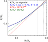 |
Fig. 17. Radial entropy profiles for a halo of 1015 M⊙ at z = 0. The black filled line shows the profile in the case of single shock at the virial radius. The blue filled line shows a profile modified with a sigmoid of the from reported in Eq. (22) and parameters shown in the figure. The vertical dotted and dashed lines mark the position of R500 and R200 respectively. The slope of the profiles can be gauged by comparison with the power laws plotted as dashed lines. |
We note that the flattening in the entropy profile could have a different physical origin from the one we have proposed above. In such a case our heuristic modeling would need to be reinterpreted within a different framework.
By combining modifications discussed in Sect. 6.1.1 with the ones that assume a larger contribution from non-thermal pressure, we come up with an entropy profile that is in good agreement with the observed one. Conversely, if we assume a smaller contribution from non-thermal pressure, we derive an entropy profile that is still steeper than the observed one but only slightly so. The difference is sufficiently small to allow us to question if the remaining deviations might be associated with issues on the observational side. We will return to this point in Sect. 6.2.
6.2. Comparison with clusters
We compare predictions based on the model presented in Sect. 5 with modifications described in Sects. 6.1.1 and 6.1.2 (see also Fig. 14) with 3 different cluster samples: HIGHMz (Riva et al. 2024), XCOP (Ghirardini et al. 2019) and REXCESS (Pratt et al. 2010) with median halo masses roughly scaling by a factor of 2, see Riva et al. (2024)5. Since the choice between larger and smaller non-thermal pressure support discussed in Sect. 6.1.2 has an impact only in the outermost regions we consider only one namely the latter.
Before proceeding with the comparison, we corrected the observed profiles for a hydro-static scaling bias of 15%, b = 0.156. We do not limit our comparison to entropy, we also include another thermo-dynamic variable, we choose density, for reason that will become apparent later. Since the remaining two variables can be derived from the former, the comparison is informative of thermo-dynamic variables in general.
In Fig. 18 we show the comparison between entropy and density profiles predicted from our model and those measured from the HIGHMz sample (Riva et al. 2024), the density profiles are renormalized through the characteristic density ρg, 500 defined by the relation: ρg, 500 = 500fbρc, where fb is the cosmic baryon fraction and ρc is the critical density of the Universe at redshift zero. The model was computed for a mass enclosed within an overdensity of 500 of 1015 M⊙. The agreement between observed data and model has been achieved by operating on the gas fraction parameters (see Eq. 18). This was not done through a formal fitting procedure but by adopting a trial and error approach. At the end of this procedure, two of the three parameters have been fixed to the following values: lm = 13.2 and lσ = 0.75. The shaded blue region is obtained by allowing the third parameter, ln, to vary in the range [−1.1, −0.3], with a central value of −0.7. This is an attempt to explain the scatter within the observed sample as a variation in ln. We note that shading stops at R ∼ 0.1 R500, for smaller radii the cooling time is shorter than the time since the gas was shock heated and entropy is reduced via radiation, something we do not account for in our model. For the radial region where the model can be meaningfully compared to observation, 0.1 R500 ≲ R ≲ R500, the agreement is quite good both for the entropy and the density (and therefore for all thermo-dynamic profiles).
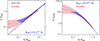 |
Fig. 18. Left panel: Entropy in units of K500 versus radius in units of R500. The three blue lines are derived from the model presented in Sect. 5 with corrections described in Sects. 6.1.1 and 6.1.2. All 3 profiles are computed assuming M500 = 1015 M⊙ and for the gas fraction parameters: lm = 13.2 and ls = −0.75. The ln parameter is set to −1.1, −0.7 and −0.3 respectively for the top, medium and bottom curves. The region between the top and bottom curves is shaded for radii where the cooling time is longer than the time since the gas was shock heated. The red shaded region is the median entropy and intrinsic scatter from the HIGHMz sample presented in Riva et al. (2024). The black dashed line shows the self-similar approximation introduced in Voit et al. (2005). Right panel: Density in units of ρg, 500 versus radius in units of R500. The three blue lines are derived from the model presented in Sect. 5 with corrections described in Sects. 6.1.1 and 6.1.2 using the same parameters for the gas fraction adopted for the entropy profile presented in the left panel. The region between the top and bottom curves is shaded for radii where the cooling time is longer than the time since the gas was shock heated. The red shaded region is the median and intrinsic scatter derived from the HIGHMz sample. |
It is worth pointing out that there is a certain degree of degeneracy between the 3 parameters describing the gas fraction versus halo mass relation. For example, a more gradual increase of the gas fraction can be obtained by increasing the value of lσ or by reducing that of lm. As already alluded to, we have chosen to reproduce the observed scatter by varying just one parameter, ln. This allows us to associate a physical interpretation with the intrinsic scatter measured in the observed sample. More specifically, objects that feature an entropy larger than average are interpreted as those for which deviation from the self-similar prediction is strongest, ln ∼ −1.1, conversely, systems that feature an entropy smaller than average, ln ∼ −0.3, are understood has having the smallest deviations from self-similarity.
Having derived a set of fg parameters that reproduces reasonably well the observed profiles of the HIGHMz sample, we perform a comparison with the lower mass samples XCOP andREXCESS. We note that in performing these comparisons we change the halo mass, which we fix to a value close to that of the median of the sample, while the parameters describing the gas fraction are fixed to the values determined for the HIGHMz sample. In Fig. 19 we show a comparison of the model with density and entropy profiles for the three datasets. For the most part, we find good agreement; we will return in the next paragraphs on minor differences. However, the most important point is that the model reproduces two key features that are found in the data. First: for each entropy profile deviations from the self-similar prediction increase with decreasing radius. Second: when comparing entropy profiles, we see that, as we go down in halo mass, observations and model feature an increasing offset with respect to the self-similar prediction. Within the model that we propose, these two features are closely connected, indeed in both instances, the growing departure from self-similarity as we move down in mass or radius stems from the increasing decoupling of baryon accretion from dark matter accretion. It is this result, much more than the quality of the individual fits, that suggests to us that baryon decoupling captures a key feature of entropy generation.
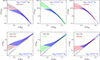 |
Fig. 19. Top panels: Gas density profiles from the model presented in Sect. 5 with corrections described in Sects. 6.1.1 and 6.1.2 for M500 = 2.5 × 10¹⁴ M⊙ (left), M500 = 5.0 × 10¹⁴ M⊙ (center), and M500 = 1015 M⊙ (right) compared with observations from the REXCESS, XCOP, and HIGHMz samples respectively. For further details see the label of Fig. 18. Bottom panels: Same as top panels but for the entropy profiles. |
The discrepancy between the modeled and observed entropy at large radii could be resolved by assuming a greater contribution from non-thermal pressure support (see Sect. 6.1.2). This would suggest a substantial non-thermal pressure fraction, ∼20% at R500. However, we are cautious about adopting this interpretation because the deviation between the model and the data (see Fig. 19, bottom panel) is at the threshold of statistical significance and background related systematics may play a role (see Rossetti et al. 2024). Therefore, we find it more prudent to conclude that, within the scope of our model, current entropy measurements are consistent with a non-thermal pressure fraction within a range of 5% to 20% at R500.
6.3. Comparison with groups
We move on to comparing our model with groups, M500 ≲ 1014 M⊙. Much less is known about these systems. While clusters thermodynamic profiles are reasonably well constrained, the same is not true for groups. More specifically there is no general consensus on the mean, median and scatter of thermodynamic profiles (see Popesso et al. 2024a, and references therein). One point recognized by all workers (see Eckert et al. 2021; Oppenheimer et al. 2021) is that group thermodynamic profiles feature a significantly larger scatter than those of clusters. We start off by making a comparison with the Sun et al. (2009) sample (see also Sun 2012), which was drawn form archival data and, although not X-ray selected in a strict sense, is X-ray bright.
In Fig. 20 we compare our model with observations from the Sun et al. (2009) sample, the only one for which density and entropy profiles are currently available. As for the comparison with the XCOP and REXCESS samples no tuning of the fg parameters is made, they are fixed to the values determined by comparison with the HIGHMz sample. Since the sample comprises mostly objects in the 5.0 × 10¹³ M⊙ to 1014 M⊙ range, we compare it with two different realizations of the model: one for M500 = 5.0 × 10¹³ M⊙ and the other for M500 = 1014 M⊙. The model shows reasonable agreement with the data. As might be expected, since the median mass of the sample is ∼7 × 10¹³ M⊙, the measured density profile is on the high side of the region predicted by the model for M500 = 5.0 × 10¹³ M⊙ and on the low side for a halo mass of M500 = 1014 M⊙. A similar variation, albeit in the opposite direction, is observed for the entropy profiles. All in all, given that the parameters describing the model where tuned by comparison with data of systems that are 10 times more massive than those considered here, the agreement is remarkable. However, before drawing more general conclusions, we must point out that there are groups that feature very different radial profiles.
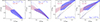 |
Fig. 20. Left panels: Density profiles predicted from our model for halo masses of 5.0 × 10¹³ M⊙ (left) and 1014 M⊙ (right), shown as blue shaded regions, compared with observations from the Sun et al. (2009) sample, shown as a red shaded region (for further details, see the label of Fig. 18). Right panels: Same as left panels but for entropy profiles. |
It has been known for some time that certain systems feature entropy profiles that display a rapid rise in the core followed by a quasi-iso-entropic range extending all the way to the outskirts. Two such systems are reported in Baldi et al. (2009), a few more can be found in Humphrey et al. (2012). More recently, several more have been identified in the XGAP sample (Eckert et al. 2024).
In the left panel of Fig. 21, we can appreciate the difference between modeled and X-ray bright profiles on one side and those reported in Eckert et al. (2024). The latter are all characterized by a rapid rise followed by a flat (quasi-iso-entropic) region. The major difference between the four XGAP profiles is the radius at which the transition occurs and the value of the entropy in the flat region. For radii smaller than 0.1−0.2 R500, the entropy is in excess of both model predictions and observed data from the Sun et al. (2009) sample. The simplest possible explanation is that these systems have recently undergone significant heating events in their cores, the likeliest culprit being the central AGN. Given that our model does not include late-time AGN heating7, radiative cooling or self regulated Chaotic Cold Accretion (e.g., Gaspari et al. 2020), it is not surprising that it fails to reproduce the Eckert et al. (2024) profiles in the central regions. By looking at the right panel of Fig. 21 we see that for radii larger than 0.2−0.3 R500, the gas fraction of these systems is consistent with the one derived from our model, suggesting that the late-time AGN heating rearranges gas only within the inner regions of the halos (see Gaspari et al. 2012).
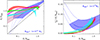 |
Fig. 21. Left panel: Radial entropy profiles. The blue and brown shaded regions respectively show the model for M500 = 1014 M⊙ and the Sun et al. (2009) profiles, already reported in Fig. 20. The red, green, violet, and cyan shaded regions represent profiles reported in Eckert et al. (2024). Right panel: Same as the left panel but for the gas fraction profiles. The gray shaded region shows the cosmic baryon fraction. |
Although our model does not include a central heating source, it is relatively straightforward to estimate the amount of heat required to account for the entropy excess and gas defect characterizing the core of the Eckert et al. (2024) systems when compared to our model or the Sun et al. (2009) sample. To first approximation, the required heat has to be comparable to the thermal energy contained within 0.1−0.3 R500. A larger heat input would lead to an entropy excess extending to larger radii. The total thermal energy is the enthalpy integrated over the region of interest, and it can be expressed as
where p500 is the characteristic pressure (see Arnaud et al. 2010, for a definition), V500 = 4/3πR5003, x = R/R500, and p(x) = p(x)/p500. We also note that within the integral, we used the symbol x rather than x to avoid confusion with the upper integration limit. A derivation of the above formula is provided in Appendix D. By carrying out the calculation we find the thermal energy within 0.1−0.3 R500 to be somewhere between 10% and 30% of the thermal energy within R500. Furthermore, since the energy required to go from a Voit (2005) profile to an XGAP one is of the order of the thermal energy content within R500, we conclude that: if, prior to the heating event, the XGAP systems had thermodynamic profiles similar to Sun et al. (2009) ones, the required energy to make the transition is about 10% to 30% of what would be needed if the starting profiles featured a self-similar behavior down to ∼0.1 R500.
7. Comparison with theoretical work
Over the past two decades, there have been several attempts to reproduce observed entropy profiles, sometimes through models, more often via simulations.
7.1. Analytical modeling
Very recently Sullivan et al. (2024) presented an analytical model for cluster entropy incorporating non-thermal pressure contributions. They find, as we do (see our Fig. 15 and their Fig. 4, left panel) that, at large radii, the predicted entropy profile is steeper than the observed one. As we have done (see Sect. 6.1) they interpret this as evidence for non thermal pressure support. More specifically they show that the predicted entropy profile can be reconciled with the observed one by allowing roughly 20% of the energy content of the gas at R500 to be in a non-thermal form (see their Fig. 4, right panel). This is quite similar to what we achieve, through a somewhat more heuristic approach, see our Fig. 16.
7.2. Simulations
In Barnes et al. (2017), the authors produce thermodynamic profiles from a large suite of simulations. Their “hot” subsample, constituted by massive systems, features a median entropy profile which, beyond the core region, is in good agreement with the self-similar prediction (Voit et al. 2005), our own model for the M500 = 1015 M⊙ case and the observed HIGHMz profile (Riva et al. 2024). Furthermore, the median entropy profile derived from their combined sample, with a median mass M500 ∼ 3 × 10¹⁴ M⊙, is in agreement with our model for the M500 = 2.5 × 10¹⁴ M⊙ case and the observed REXCESS profile (see Fig. 22, left panel). According to the authors, the ability of their simulations to reproduce deviations from self-similarity observed in the data has to do with the inclusion of feedback from AGN. Unfortunately, from their paper it is not possible for us to determine how feedback actually achieves that objective.
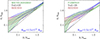 |
Fig. 22. Left panel: Radial entropy profiles for the combined sample extracted from the MACSIS and BAHAMAS simulations (Barnes et al. 2017) compared with the one derived from our model for M500 = 2.5 × 10¹⁴ M⊙ and with the observed REXCESS profile. Right panel: Radial entropy profiles from the FLAMINGO simulation for objects in the M500 = 1014 − 1014.5 M⊙ mass bin compared with the one derived from our model for M500 = 2.5 × 10¹⁴ M⊙ and with the observed REXCESS profile. |
Recently Braspenning et al. (2024) have published thermodynamic profiles from the FLAMINGO suite of simulations (Schaye et al. 2023). Their entropy profile for the M500 = 1014 − 1014.5 M⊙ mass bin is compared to our prediction for M500 = 2.5 × 10¹⁴ M⊙ and the REXCESS observed profile in Fig. 22, right panel. As we can see, the FLAMINGO profile appears to be flatter than our own and, more importantly, of the observed profile. The tendency of simulated entropy profiles to be flatter than observed ones has been noted before (see Altamura et al. 2023). As discussed by these authors, there are several possible explanations. One possibility is that numerical viscosity and conduction, present in SPH simulations but absent from our model, favor mixing and heat transfer in the gas, which in turn lead to a reduction of the entropy gradient (see Fig. 6 of Altamura et al. 2023). As discussed in detail in Molendi et al. (2023) (see also Zhuravleva et al. 2019) there is significant evidence that both conduction and viscosity are heavily suppressed in the ICM.
7.3. Scaling relations
A different kind of connection can be made between our model and a phenomenological approach that has been pursued over the past two decades. Several authors have attempted to reduce the scatter in scaling relations and thermodynamic profiles that is left after applying self-similar scaling, by introducing modifications to the scaling laws (see Lovisari & Maughan 2022, for a review). Pratt et al. (2010) have shown that the scatter on the entropy profile of REXCESS clusters can be substantially reduced by multiplying it by the gas mass fraction. Recently, Ettori et al. (2023), have identified a correction scheme that modifies the self-similar predictions through two quantities: the gas mass fraction and the ratio between the global spectroscopic temperature and the temperature at R500, with the former providing the most significant contribution. Interestingly, the authors derive a gas fraction versus halo mass relation that is broadly consistent with the one we derive by fitting the thermodynamic profiles of massive halos, see Sect. 6.2 and Fig. 23. It would therefore seem that a model based on baryon decoupling can provide a physical basis for the phenomenological findings reported in Pratt et al. (2010) and Ettori et al. (2023).
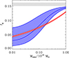 |
Fig. 23. Gas fraction as a function of halo mass. The solid blue lines show the profiles for the three choices of parameters adopted to fit cluster and group thermodynamic profiles. The blue shaded region spans the region between the different profiles. The red shaded region shows the gas fraction derived in Ettori et al. (2023) to minimize scatter in cluster scaling relations. The gray shaded region shows the cosmic baryon fraction. |
Another connection can be made between our model and scaling relations. In Bower et al. (2008), the authors employ a semi-analytical model to investigate the luminosity temperature relation. To bring predictions into agreement with observations, they require the gas fraction in less massive halos to be smaller than in more massive ones. Intriguingly, they point out that the major problem for their model is the high level of heating required from the AGN, which follows from assuming that the heating occurs after the system has collapsed. As discussed in Sect. 6.3, baryon decoupling offers a simple and viable solution to this problem: the low gas fraction in less massive systems is achieved by delaying baryon infall rather than by ejecting the gas.
8. Discussion
We have shown that a simple model based on baryon decoupling is consistent with thermodynamic profiles at cluster scale and provides valuable insight on processes operating at the group scale. In this section we explore the implications of our results. Before doing so we take care of an important preliminary issues.
8.1. Evidence against a scale of massive gas ejection
Inspection of Fig. 23 reveals that the deviations from self-similarity in entropy at the cluster scale (see Figs. 18 and 19) stem from a phase of extremely low gas content centered around 1013 M⊙. According to our model, halos at this mass scale are missing between 50% and 90% of their baryons, corresponding to a gas fraction ranging between 2% and 8%. As discussed in Sect. 5.1, we interpret this severe depletion as the result of a phase of massive baryon evacuation. This finding is quite significant, and before proceeding, we must critically evaluate whether it aligns or conflicts with current observational data.
The gas content of halos around 1013 M⊙ remains largely unknown, primarily because the relevant measurements are extremely challenging to secure (see Tumlinson et al. 2017, and references therein). In a recent and brave attempt, Zhang et al. (2024b), stacking X-ray emission around ∼105 SDD galaxies, found that the gas fraction within R500 of halos of mass ∼1013 M⊙ is in the order of 0.02−0.03, which is well within the range of our estimates. A detailed analysis of the systematics associated to the stacking procedure (Popesso et al. 2024b), while highlighting several criticalities inherent to the technique, confirm the Zhang et al. (2024b) result, albeit with significantly larger uncertainties: fg(R < R500)∼0.00 − 0.07 (Popesso et al. 2024c, see their Fig. 4). It is also worth pointing out that, in the few cases where measurements are available on individual systems, they are likely not representative of the general population (see Popesso et al. 2024a, and references therein). Furthermore, we do have indirect evidence that large amounts of enriched gas are expelled at these scales, (see Molendi et al. 2024). We conclude that, at least for the moment, the little observational evidence that is available does not challenge our inference of substantial gas mass ejection at the 1013 M⊙ scale.
8.2. Understanding entropy in massive halos
The success of our model in reproducing thermodynamic profiles of massive halos allows us make a few inferences about the underlying physics. The rough agreement between observed and modeled entropy and density in the outskirts of massive clusters (see Fig. 6), combined with evidence for moderate non-thermal pressure support in the R500 − R200, see discussion at the end of Sect. 6.2, tells us that, to first order: (1) entropy is generated close to the virial radius, through an accretion shock; (2) the processes operating in such a shock, whatever they may be, must convert the bulk of the kinetic energy into thermal energy in a relatively narrow radial range.
The formation of an accretion shock at the virial radius can be understood in relatively simple terms. We know that within our Universe halos virialize at a specific overdensity (see Voit 2005, and references therein). In a collisionless fluid, such as dark matter, virialization is the process by which matter reorganizes itself by converting its velocity from radial to isotropic. This leads to a sharp increase in matter density around the virial radius. Since baryons are as affected by gravity as dark matter is, they also redistribute themselves in phase space like dark matter. However, unlike dark matter, baryons are collisional, which means that the interaction between low density baryons that are radially infalling and higher density baryons on isotropic orbits results in the formation of a shock front. It is for this reason that, as the halo mass grows by orders of magnitude, the shock tracks the virial radius as it moves outwards. Simulations (e.g., Vazza et al. 2009) suggest the gas undergoes multiple shocks spread out over a large radial range. However, from the point of view of entropy generation, the bulk is likely produced in just one shock, roughly located at the virial radius.
On the second point there is much less we can say. More than 60 years after their discovery, collisionless shocks in space are still very much the mystery they have always been (see Goodrich et al. 2023, and references therein). While we can infer that accretion shocks must be quite efficient in converting kinetic energy into thermal energy, we have little to say about how this is achieved.
The good agreement between observed thermodynamic profiles and predictions from our model, over a broad range of halo masses (see Figs. 18, 19 and 20), tells us that the modifications to the thermodynamics of massive halos, with respect to the self-similar model, can be explained through baryon decoupling. More specifically, for halo masses larger than ∼1013 M⊙, accreted matter contains a baryon fraction that is smaller than the cosmic one, this results in an increase in entropy with respect to the self-similar model. Since the baryon deficiency is larger for accretion on smaller halos: (1) for any given halo, the deviation in the radial profiles with respect to the self-similar prediction is larger at smaller radii and (2) the thermodynamic profiles of less massive halos feature a general offset, with respect to the self-similar model, that is larger than in more massive ones. It is this result, much more than the quality of the individual fits, that suggests to us that baryon decoupling captures a fundamental feature of entropy generation.
8.3. Non-thermal pressure support
As discussed in Sects. 6.1.2, 6.2 and 7.1, within our and similar models (e.g., Sullivan et al. 2024), there is a tight connection between non-thermal pressure support and the slope of the entropy profile in the outer regions of clusters, with steeper profiles requiring a smaller non-thermal pressure fraction. Current estimates place the non-thermal pressure fraction at R500 between 5% and 20%, while the entropy profile slopes in the R500 − R200 range are estimated to be between 0.7 and 0.9. The limitations of current measurements for both parameters hinder our ability to use one to precisely constrain the other, leaving the radial extent of the shock-heated region uncertain.
Progress will require new and improved measurements of the entropy or the non-thermal pressure in cluster outskirts. Entropy profiles could be secured through a combination of high sensitivity surface brightness measurements in X-rays and Sunyaev-Zeldovich (SZ) observation in the sub-millimeter range. The former with missions such as AXIS (Reynolds et al. 2024), recently selected for a phase A study by NASA and through the WFI experiment on board the L-class mission NewAthena currently under study by ESA; the latter with future facilities such as AtLAST (Di Mascolo et al. 2024). The most effective way of estimating non-thermal pressure is through high resolution spectroscopic observations. The currently operational XRISM observatory (Tashiro et al. 2018) might provide some first results, much more will become possible with the XIFU experiment (Peille et al. 2025) on board NewAthena.
8.4. Baryon decoupling versus pre-heating
The baryon decoupling mechanism we propose exhibits substantial differences from the pre-heating models of the early 2000s, see Sect. 4. In our model, in massive halos, Mh ∼ 1014 − 1015 M⊙, almost all the heat conferred to the gas is of gravitational nature. Although feedback processes remain crucial, they require comparatively little energy; the key is to remove gas from shallow potential wells and allow gravity to do the rest. The situation is radically different at the low mass end, Mh ∼ 1013 M⊙, here the energy of the expelled gas is sufficient to prevent, at least in part, its re-accretion.
8.5. Gas fraction parametrization
The broad range of minimum baryon content suggested by our fits, fg/fb = 0.1 − 0.5 for Mh ∼ 1013 M⊙, see Fig. 23, likely follows from the stochastic nature of accretion onto the halo and of AGN feedback processes. As far as the mass range over which this minimum is reached, it cannot be estimated from our fits alone because they are essentially insensitive to accretion on halos less massive than about Mh ∼ 1013 M⊙. As discussed in Sect. 5.4, see also Figs. 9 and 10, the presence of a minimum in the gas fraction versus halo mass relation leads to a marked change in slope in the radial entropy profile. As it happens, for more massive halos (see Fig. 19), this variation occurs in the core of these systems where gas cooling becomes important and, as indicated by the comparison with data, washes it away. For less massive systems (see Fig. 19), although the variation occurs beyond the region where cooling becomes important, it is still within the reach of feedback from the SMBH (Gaspari et al. 2014) operating at late-times, that is, when the halo mass has grown well beyond 1013 M⊙.
The minimum on 10lm can be set at ∼5 ⋅ 1012 M⊙ by recalling that the stellar mass fraction versus halo mass relation reaches a maximum around a few 1012 M⊙, for halos at z ∼ 2 − 3, which are the progenitors of current groups and clusters, suggesting that up to this scale feedback effects do not prevent star formation by heating up the gas and therefore are unlikely to heat it up to virial temperatures. The maximum can be estimated at ∼3 ⋅ 1013 M⊙ by noting that observed entropy profiles at the cluster mass scale show no evidence of the rapid change in slope discussed earlier in this subsection.
8.6. Scatter and bias in group samples
Our analysis indicates that reproducing the scatter in thermodynamic profiles at the cluster scale requires the gas fraction to exhibit an increasing scatter with decreasing halo mass, as illustrated in Fig. 23. We propose that this trend arises from a shift in accretion modes. At the “ejection” scale, around 1013 M⊙, outbursts from the central galaxy’s supermassive black hole (SMBH) expel gas from the halo. Due to the stochastic nature of these outbursts, different systems experience significantly varying levels of baryon loss. Over cosmic time, as the halo mass increases, the source of re-accreted baryons changes. Initially, the re-accreted material originates primarily from the halo’s own ejected baryons. However, as the halo mass continues to grow, re-accreted baryons increasingly come from a large number of smaller halos. Since individual halos expel varying amounts of gas, this process progressively reduces the scatter in the total amount of accreted gas, leading to the trend observed in Fig. 23.
Whatever the origin of the increase in scatter with decreasing halo mass, it implies that for Mh ⪅ 5 ⋅ 1013 M⊙, a substantial portion of the population must have a very low baryon fraction. Consequently, any X-ray selected group sample is likely to be significantly biased. Notably, a similar conclusion has been reached by other studies using entirely independent methods (see Popesso et al. 2024a, and references therein). It is also important to note that this bias may be even more pronounced than our model predicts, as it does not account for late-time AGN heating effects, which are clearly observed (see Eckert et al. 2024).
8.7. Transitions
From an observational point of view, the “ejection” scale around 1013 M⊙ provides a physically meaningful divide between lower mass halos dominated by individual galaxies and higher mass multi galaxy systems. Below this threshold, stellar mass builds up rapidly from the accretion of cold gas, above it, the accreted gas is predominantly hot, leading to a sharp decline in the central galaxy’s star formation rate, often to the point of near cessation. As halo mass increases beyond the ejection scale, the stellar mass associated with sub-halos becomes more prominent, making the system more easily identifiable as a multi-galaxy system (see Fig. 9 of Coupon et al. 2015).
Baryons at the group and cluster scales clearly show significant differences. Groups feature a larger scatter in their properties, their baryon fraction is smaller and late-time heating from the central AGN contributes more significantly to their overall thermodynamic structure. That said, it is important to recognize that there is no clear separation between these two regimes. As far as we can tell, all these properties slowly vary with halo mass. In this sense the group/cluster scale separation appears to be less fundamental than the galaxy/group one, which is characterized by a change of the primary accretion mode from cold to hot.
8.8. Active galactic nucleus heating
In the framework we have sketched, the group and cluster scales (Mh ≳ 1013 M⊙) can be viewed as the mass range over which halos reacquire expelled baryons. One may ask why the AGN feedback that is so effective in ejecting baryons in halos in the few 1012 M⊙ to 1013 M⊙ range seems to be incapable of doing so in more massive halos. The answer likely lies in the combination of two factors. One, as shown by the shut down of the star formation process (see Sect. 5 and references therein), the cold gas reservoir from which stars are formed and the black hole is fed, dries out at these scales never to be replenished. Two, as discussed in Gaspari et al. (2014), the maximum energy that can be extracted from the central AGN is comparable to the binding energy of poor groups. Thus, as halos grow in size, SMBH heating is restricted to progressively smaller self-similar radii. Although AGN feedback is incapable of baryon evacuation at the group and cluster scales, it does play a role in shaping the thermodynamics of these systems. At the group scale, where baryon decoupling is more substantial, it provides enough heat to reshape the thermodynamic profiles out to about a 1/5 of the virial radius (see Sect. 6.1.1). At the cluster scale its effects are contained within the core.
9. Summary
In this paper, we have presented a semi-analytical model that builds on work from the early 2000s. The model assumes that the bulk of the entropy of the hot gas in massive halos is generated near the virial shock. We investigated how differences between entropy profiles predicted under gravitational collapse alone (known as self-similar profiles) and observed profiles can be reconciled by incorporating feedback processes. After demonstrating that adding pre-heating to the entropy generation process reduces, but does not fully resolve, the discrepancy between the model and observed data, we explored an alternative form of feedback. The core idea of our new approach is that by decoupling baryon accretion from dark matter accretion, we can reduce the density and increase the entropy of the accreted gas. We implemented this “baryon decoupling” concept through a parametric model for the gas fraction versus halo mass relation. Our main findings are summarized as follows:
-
Our model provides a simple explanation for the effectiveness of gas fraction rescaling in reducing the scatter observed in entropy profiles of galaxy clusters.
-
The difference in slope between predicted, dlnK/dlnr ∼ 1.2, and observed, dlnK/dlnr ∼ 0.8, entropy profiles of massive clusters at large radii can be reconciled, for the better part, through the adoption of a heuristic model and the assumption that entropy is generated over a radial range rather than just at the virial radius. Improved measurements of the entropy profile and the non-thermal pressure support in cluster outskirts are needed to further constrain the size of this region.
-
Entropy and density profiles generated from a single set of parameters describing the gas fraction versus halo mass relation are in good agreement with observations from three different datasets that fully sample the cluster mass scale.
-
Our model reproduces the growing departure from self-similarity observed in the data when moving inward in individual profiles and down in mass across different profiles. It is this result more than any other that suggests that baryon decoupling captures a key feature of entropy generation.
-
In our model, deviations from self-similarity in entropy at the cluster scale stem from a phase of extremely low gas content centered around 1013 M⊙. We estimate that halos at this mass scale are missing between 50% and 90% of their baryons, corresponding to a gas fraction ranging between 2% and 8%.
-
Our model reproduces entropy profiles of X-ray bright groups but not those of “quasi-isoentropic” groups. The latter clearly require late-time heating from the central AGN, which we do not include. Baryon decoupling does, however, significantly reduce the amount of AGN heating that is required.
-
The increase of scatter in the gas fraction, when moving down in halo mass results from the reduction in the number of halos from which the re-accreted gas has previously been expelled.
-
To reproduce the scatter in entropy profiles at the cluster scale, the gas fraction at the group scale must exhibit large variations. This implies that X-ray selected samples are likely to be significantly biased against gas-poor groups.
-
The “ejection” scale around 1013 M⊙ that we have identified by modeling the gas fraction versus halo mass relation provides a physically meaningful divide between lower mass halos dominated by individual galaxies and higher mass multi-galaxy systems. Below this threshold, stellar mass builds up rapidly from the accretion of cold gas, and above it, the accreted gas is predominantly hot, and the central galaxy star formation rate is reduced to the point of almost being shut off.
-
The AGN feedback that is so effective in ejecting baryons in halos in the few 1012 M⊙ to 1013 M⊙ range is incapable of doing so in more massive halos for two reasons: The cold gas reservoir from which stars are formed and the black hole is fed dries out at these scales, and the maximum energy that can be extracted from the central AGN is comparable to the binding energy of poor groups.
What we have conducted in this paper might be described as a “thought experiment”. We set out to determine whether a single modification, the decoupling of baryon accretion from dark matter accretion, could account for a specific phenomenon, the observed deviation of entropy profiles from the self-similar prediction. Remarkably, baryon decoupling proves effective in explaining much of the behavior we sought to understand. While certain aspects inevitably require more complex modifications, the simplicity of our model offers valuable insights and a clearer understanding of the underlying processes.
It is important to note that in studies of the intra-cluster medium (ICM), the term “entropy” refers to a quantity related to the thermodynamic specific entropy, s: s = 3/2 kblnK + const (see Eqs. 9 and 10 in Donahue & Voit 2022). Additionally, specific entropy is an intensive variable.
The v subscript is present on the right hand side of the equation to highlight that this is the entropy generated at a time when the virial radius was going through the radius R, it is dropped on the left hand side of the equation because what we wish to emphasize in this case is that K(R) is the entropy at a generic radius R.
As the attentive reader will have undoubtedly realized, the slopes of observed and predicted profiles differ significantly. This point is discussed at length in Sect. 6.1.
The factor b is defined through the relationship b = 1 − MHSE/MT, where MHSE is the mass derived from the hydrostatic equilibrium equation and MT is the total mass of the halo; to first approximation, the non-thermal pressure fraction, defined as the ratio of non-thermal pressure to total pressure is equal to the b parameter (Eckert et al. 2019).
All entropy profiles have been extracted from Riva et al. (2024), density profiles are extracted from the papers where they were first presented.
As discussed in Sect. 5, our model assumes that early-time AGN feedback is responsible for expelling large amounts of gas in halos with masses around 1013 M⊙. It does not include a treatment for late-time AGN feedback at the group or cluster scales.
Acknowledgments
We are grateful to the referee, Mark Voit, for helpful comments that improved the quality of our manuscript. S.M. thanks former Master student Giacomo Aprea for his contribution to this project. We acknowledge financial support from INAF mainstream project No.1.05.01.86.13. M.G. acknowledges support from the ERC Consolidator Grant BlackHoleWeather (101086804). L.L. acknowledges support from INAF grant 1.05.12.04.01. PT acknowledges support from the Next Generation European Union PRIN 2022 20225E4SY5 – “From ProtoClusters to Clusters in one Gyr”.
References
- Altamura, E., Kay, S. T., Bower, R. G., et al. 2023, MNRAS, 520, 3164 [CrossRef] [Google Scholar]
- Arnaud, M., Pratt, G. W., Piffaretti, R., et al. 2010, A&A, 517, A92 [CrossRef] [EDP Sciences] [Google Scholar]
- Baldi, A., Forman, W., Jones, C., et al. 2009, ApJ, 694, 479 [Google Scholar]
- Balogh, M. L., Babul, A., & Patton, D. R. 1999, MNRAS, 307, 463 [Google Scholar]
- Barnes, D. J., Kay, S. T., Henson, M. A., et al. 2017, MNRAS, 465, 213 [Google Scholar]
- Behroozi, P. S., Wechsler, R. H., & Conroy, C. 2013, ApJ, 770, 57 [NASA ADS] [CrossRef] [Google Scholar]
- Behroozi, P., Wechsler, R. H., Hearin, A. P., & Conroy, C. 2019, MNRAS, 488, 3143 [NASA ADS] [CrossRef] [Google Scholar]
- Binney, J., & Tremaine, S. 1987, Galactic Dynamics (Princeton: Princeton University Press) [Google Scholar]
- Borgani, S., Governato, F., Wadsley, J., et al. 2002, MNRAS, 336, 409 [NASA ADS] [CrossRef] [Google Scholar]
- Borgani, S., Finoguenov, A., Kay, S. T., et al. 2005, MNRAS, 361, 233 [NASA ADS] [CrossRef] [Google Scholar]
- Bower, R. G., McCarthy, I. G., & Benson, A. J. 2008, MNRAS, 390, 1399 [NASA ADS] [Google Scholar]
- Braspenning, J., Schaye, J., Schaller, M., et al. 2024, MNRAS, 533, 2656 [NASA ADS] [CrossRef] [Google Scholar]
- Coupon, J., Kilbinger, M., McCracken, H. J., et al. 2012, A&A, 542, A5 [NASA ADS] [CrossRef] [EDP Sciences] [Google Scholar]
- Coupon, J., Arnouts, S., van Waerbeke, L., et al. 2015, MNRAS, 449, 1352 [NASA ADS] [CrossRef] [Google Scholar]
- Cowley, W. I., Caputi, K. I., Deshmukh, S., et al. 2018, ApJ, 853, 69 [NASA ADS] [CrossRef] [Google Scholar]
- Di Mascolo, L., Perrott, Y., Mroczkowski, T., et al. 2024, ArXiv e-prints [arXiv:2403.00909] [Google Scholar]
- Donahue, M., & Voit, G. M. 2022, Phys. Rep., 973, 1 [NASA ADS] [CrossRef] [Google Scholar]
- Dupourqué, S., Clerc, N., Pointecouteau, E., et al. 2024, A&A, 687, A58 [NASA ADS] [CrossRef] [EDP Sciences] [Google Scholar]
- Eckert, D., Ghirardini, V., Ettori, S., et al. 2019, A&A, 621, A40 [NASA ADS] [CrossRef] [EDP Sciences] [Google Scholar]
- Eckert, D., Gaspari, M., Gastaldello, F., Le Brun, A. M. C., & O’Sullivan, E. 2021, Universe, 7, 142 [NASA ADS] [CrossRef] [Google Scholar]
- Eckert, D., Gastaldello, F., O’Sullivan, E., et al. 2024, Galaxies, 12, 24 [NASA ADS] [CrossRef] [Google Scholar]
- Ettori, S., Ghirardini, V., Eckert, D., et al. 2019, A&A, 621, A39 [NASA ADS] [CrossRef] [EDP Sciences] [Google Scholar]
- Ettori, S., Lovisari, L., & Eckert, D. 2023, A&A, 669, A133 [NASA ADS] [CrossRef] [EDP Sciences] [Google Scholar]
- Gaspari, M., Brighenti, F., & Temi, P. 2012, MNRAS, 424, 190 [NASA ADS] [CrossRef] [Google Scholar]
- Gaspari, M., Brighenti, F., Temi, P., & Ettori, S. 2014, ApJ, 783, L10 [NASA ADS] [CrossRef] [Google Scholar]
- Gaspari, M., Eckert, D., Ettori, S., et al. 2019, ApJ, 884, 169 [NASA ADS] [CrossRef] [Google Scholar]
- Gaspari, M., Tombesi, F., & Cappi, M. 2020, Nat. Astron., 4, 10 [Google Scholar]
- Ghirardini, V., Ettori, S., Eckert, D., & Molendi, S. 2019, A&A, 627, A19 [NASA ADS] [CrossRef] [EDP Sciences] [Google Scholar]
- Ghizzardi, S., Molendi, S., van der Burg, R., et al. 2021, A&A, 646, A92 [NASA ADS] [CrossRef] [EDP Sciences] [Google Scholar]
- Girelli, G., Pozzetti, L., Bolzonella, M., et al. 2020, A&A, 634, A135 [NASA ADS] [CrossRef] [EDP Sciences] [Google Scholar]
- Goodrich, K., Schwartz, S., Wilson, L., et al. 2023, BAAS, 55, 134 [Google Scholar]
- Humphrey, P. J., Buote, D. A., Brighenti, F., et al. 2012, ApJ, 748, 11 [NASA ADS] [CrossRef] [Google Scholar]
- Kaiser, N. 1986, MNRAS, 222, 323 [Google Scholar]
- Kaiser, N. 1991, ApJ, 383, 104 [NASA ADS] [CrossRef] [Google Scholar]
- Leauthaud, A., Tinker, J., Bundy, K., et al. 2012, ApJ, 744, 159 [Google Scholar]
- Legrand, L., McCracken, H. J., Davidzon, I., et al. 2019, MNRAS, 486, 5468 [NASA ADS] [CrossRef] [Google Scholar]
- Lovisari, L., & Maughan, B. J. 2022, in Handbook of X-ray and Gamma-ray Astrophysics, eds. C. Bambi, & A. Sangangelo, 65 [Google Scholar]
- Lovisari, L., Ettori, S., Rasia, E., et al. 2024, A&A, 682, A45 [NASA ADS] [CrossRef] [EDP Sciences] [Google Scholar]
- McCarthy, I. G., Babul, A., & Balogh, M. L. 2002, ApJ, 573, 515 [Google Scholar]
- McCarthy, I. G., Balogh, M. L., Babul, A., Poole, G. B., & Horner, D. J. 2004, ApJ, 613, 811 [NASA ADS] [CrossRef] [Google Scholar]
- Molendi, S., De Grandi, S., Rossetti, M., et al. 2023, A&A, 670, A104 [NASA ADS] [CrossRef] [EDP Sciences] [Google Scholar]
- Molendi, S., Ghizzardi, S., De Grandi, S., et al. 2024, A&A, 685, A88 [NASA ADS] [CrossRef] [EDP Sciences] [Google Scholar]
- Moster, B. P., Naab, T., & White, S. D. M. 2013, MNRAS, 428, 3121 [Google Scholar]
- Muñoz-Echeverría, M., Macías-Pérez, J. F., Pratt, G. W., et al. 2024, A&A, 682, A147 [NASA ADS] [CrossRef] [EDP Sciences] [Google Scholar]
- Navarro, J. F., Frenk, C. S., & White, S. D. M. 1997, ApJ, 490, 493 [Google Scholar]
- Nicastro, F., Fang, T., & Mathur, S. 2022, ArXiv e-prints [arXiv:2203.15666] [Google Scholar]
- Oppenheimer, B. D., Babul, A., Bahé, Y., Butsky, I. S., & McCarthy, I. G. 2021, Universe, 7, 209 [NASA ADS] [CrossRef] [Google Scholar]
- Peille, P., Barret, D., Cucchetti, E., et al. 2025, ArXiv e-prints [arXiv:2502.10866] [Google Scholar]
- Ponman, T. J., Sanderson, A. J. R., & Finoguenov, A. 2003, MNRAS, 343, 331 [NASA ADS] [CrossRef] [Google Scholar]
- Popesso, P., Biviano, A., Bulbul, E., et al. 2024a, MNRAS, 527, 895 [Google Scholar]
- Popesso, P., Marini, I., Dolag, K., et al. 2024b, A&A, submitted [arXiv:2411.16546] [Google Scholar]
- Popesso, P., Biviano, A., Marini, I., et al. 2024c, A&A, submitted [arXiv:2411.16555] [Google Scholar]
- Pratt, G. W., Arnaud, M., & Pointecouteau, E. 2006, A&A, 446, 429 [NASA ADS] [CrossRef] [EDP Sciences] [Google Scholar]
- Pratt, G. W., Arnaud, M., Piffaretti, R., et al. 2010, A&A, 511, A85 [NASA ADS] [CrossRef] [EDP Sciences] [Google Scholar]
- Pringle, J. E., & King, A. 2007, Astrophysical Flows (Cambridge: Cambridge University Press) [Google Scholar]
- Rasia, E., Tormen, G., & Moscardini, L. 2004, MNRAS, 351, 237 [NASA ADS] [CrossRef] [Google Scholar]
- Reines, A. E., & Volonteri, M. 2015, ApJ, 813, 82 [NASA ADS] [CrossRef] [Google Scholar]
- Reynolds, C. S., Miller, E. D., Hodges-Kluck, E., et al. 2024, SPIE Conf. Ser., 13093, 1309328 [Google Scholar]
- Riva, G., Pratt, G. W., Rossetti, M., et al. 2024, A&A, 691, A340 [NASA ADS] [CrossRef] [EDP Sciences] [Google Scholar]
- Rossetti, M., Eckert, D., Gastaldello, F., et al. 2024, A&A, 686, A68 [NASA ADS] [CrossRef] [EDP Sciences] [Google Scholar]
- Salcido, J., Bower, R. G., & Theuns, T. 2020, MNRAS, 491, 5083 [NASA ADS] [CrossRef] [Google Scholar]
- Schaye, J., Kugel, R., Schaller, M., et al. 2023, MNRAS, 526, 4978 [NASA ADS] [CrossRef] [Google Scholar]
- Shuntov, M., McCracken, H. J., Gavazzi, R., et al. 2022, A&A, 664, A61 [NASA ADS] [CrossRef] [EDP Sciences] [Google Scholar]
- Sullivan, A., Shabala, S., Power, C., Bottrell, C., & Robotham, A. 2024, PASA, 41, e064 [Google Scholar]
- Sun, M. 2012, New J. Phys., 14, 045004 [NASA ADS] [CrossRef] [Google Scholar]
- Sun, M., Voit, G. M., Donahue, M., et al. 2009, ApJ, 693, 1142 [NASA ADS] [CrossRef] [Google Scholar]
- Tashiro, M., Maejima, H., Toda, K., et al. 2018, Proc. SPIE, 10699, 1069922 [Google Scholar]
- Tozzi, P., & Norman, C. 2001, ApJ, 546, 63 [NASA ADS] [CrossRef] [Google Scholar]
- Tumlinson, J., Peeples, M. S., & Werk, J. K. 2017, ARA&A, 55, 389 [Google Scholar]
- Vazza, F., Brunetti, G., Kritsuk, A., et al. 2009, A&A, 504, 33 [NASA ADS] [CrossRef] [EDP Sciences] [Google Scholar]
- Voit, G. M. 2005, Rev. Mod. Phys., 77, 207 [Google Scholar]
- Voit, G. M., Balogh, M. L., Bower, R. G., Lacey, C. G., & Bryan, G. L. 2003, ApJ, 593, 272 [NASA ADS] [CrossRef] [Google Scholar]
- Voit, G. M., Kay, S. T., & Bryan, G. L. 2005, MNRAS, 364, 909 [NASA ADS] [CrossRef] [Google Scholar]
- Wicker, R., Douspis, M., Salvati, L., & Aghanim, N. 2023, A&A, 674, A48 [NASA ADS] [CrossRef] [EDP Sciences] [Google Scholar]
- Zhang, H., Behroozi, P., Volonteri, M., et al. 2024a, ArXiv e-prints [arXiv:2409.16347] [Google Scholar]
- Zhang, Y., Comparat, J., Ponti, G., et al. 2024b, A&A, 690, A267 [NASA ADS] [CrossRef] [EDP Sciences] [Google Scholar]
- Zhuravleva, I., Churazov, E., Schekochihin, A. A., et al. 2019, Nat. Astron., 3, 832 [Google Scholar]
Appendix A: Deriving dlnKv/dlnMh
In this appendix, we derive the relation presented in Eq. 11. We start off with the expression for Kv in Eq. 10. As a first step, we compute the natural logarithm of Kv:
![$$ \begin{aligned} \ln K_{\rm v} = \ln \left[{1 \over 3} \, (\pi G^2)^{2/3} \, f_{\rm b}^{-2/3}\right] \, + \ln \left({M_{\rm h} \over \dot{M}_{\rm h}}\right)^{2/3} + \ln M_{\rm h}^{2/3}. \end{aligned} $$](/articles/aa/full_html/2025/07/aa53299-24/aa53299-24-eq51.gif)
Next, by noting that  can be rewritten as t dlnt/dlnMh and defining α as α ≡ dlnMh/dlnt, we get
![$$ \begin{aligned} \ln K_{\rm v} = \ln \left[{1 \over 3} \, (\pi G^2)^{2/3} \, f_{\rm b}^{-2/3}\right] + {2 \over 3} \left(\ln t - \ln \alpha + \ln M_{\rm h}\right). \end{aligned} $$](/articles/aa/full_html/2025/07/aa53299-24/aa53299-24-eq53.gif)
Next, we compute the derivative of lnKv with respect to lnMh:
which simplifies to

Appendix B: Applying hydrostatic equilibrium
In this appendix we present the numerical method we have adopted to derive thermodynamic profiles under the condition of hydrostatic equilibrium.
B.1. Thermodynamic variables at the virial radius
We start by deriving expressions for thermodynamic variables at the shock radius, which is assumed to coincide with the virial radius, Rv. Assuming a strong shock, the following relation holds:

where ρg, u and ρg, d are respectively the gas density upstream and downstream of the shock. By combining Eq. B.1 with equations describing the mass flow (Eq. 1) and the velocity of the accreted gas (Eq. 2), we derive the following expression:

where Mh is the halo mass and  the gas accretion rate. Combining energy conservation (Eq. 3) with the equation describing the velocity of the accreted gas (Eq. 2) we derive the following expression for the gas temperature at the virial radius:
where kb is the Boltzmann constant, μ the mean molecular weight of the gas and mp the proton mass. Assuming our gas obeys the equation of state for a monoatomic gas,
and making use of Eqs. B.2 and B.3, we derive an expression for the gas pressure at the virial radius:
Similarly, starting from the definition of entropy:
and making use of Eqs. B.2 and B.3 we get the following expression for the entropy at the virial radius:
B.2. Hydrostatic equilibrium equation
The next step is to take the commonly adopted form of the equation of hydrostatic equilibrium equation,
and, in light of the power-law like nature of thermodynamic profiles, rewrite it as
Next, following (Tozzi & Norman 2001), we rewrite Eq. B.9 by dividing each variable by its value at the virial radius:
where
By plugging Eq. B.3 into Eq. B.11, we get

An advantage of Eq. B.10 is that it allows us to assign at a glance a physical interpretation to the numerical term, C = 3. Since, for x = 1, all terms on the right side of the equation are 1, −3 is the slope of the lnp versus lnx relation at the virial radius.
Equations B.1, B.3, B.4, B.6 completely describe physical conditions at the virial radius. By imposing hydrostatic equilibrium, we relate variations in thermodynamic quantities with the quantities themselves and, since these quantities are known at the virial radius, so are the variations which relate them. Furthermore, by rewriting the hydrostatic equilibrium equation in terms of dlnPg/dlnR the two terms on the right hand side of Eq. B.9 become proportional to one another when we evaluate Eq. B.9 at the virial radius (see Eq. B.3). This is what allows us to establish that dlnPg/dlnR computed at Rv is a constant.
Finally, following (Tozzi & Norman 2001), we rewrite the normalized temperature in Eq. B.10 in terms of normalized pressure and entropy:
where k = K/Kv.
B.3. Gas mass equation
The next step is to take the differential relation between gas mass within a given radius and the gas density at that radius,
and subject it to the same sort of massaging we applied to the hydrostatic equilibrium equation. We start by rewriting Eq. B.14 through variables that are one at the virial radius
where
We rewrite Cg in a more convenient form:
Finally, as we have done for the pressure gradient, we rewrite Eq. B.15 in terms of natural logarithms and express density in terms of pressure and entropy:
As for the hydrostatic equilibrium equation, see Eq. B.10, this form allows us to understand that Cg is the slope of the lnMg versus lnR relation at the virial radius:
B.4. Entropy equation
In our model, entropy generation occurs only at the virial (shock) radius, this implies that any further evolution of the gas will be adiabatic. The gas may compress or expand to obey the hydrostatic equation, but it will not change its entropy. This implies that the entropy of a gas element within the halo can be expressed as a function of the halo mass and gas accretion rate at the time the element was shock heated, see Eq. 8. In differential terms, we may say that the infinitesimal increase in entropy is determined by the infinitesimal increase in gas mass. Thus, the variable dlnK/dlnMg will not depend on the radius within the halo where the infinitesimal gas element eventually resides but only on the halo mass at the time the gas was accreted. Furthermore, once a description of how the gas mass, Mg, varies with the halo mass is provided, Mg = Mg(Mh) (see Eq. 9 for the self-similar case and Eq. 19 for the baryon decoupling case), dlnK/dlnMg is completely specified and can be readily computed from Mh, which in mathematical terms is
B.5. Numerical solution
The differential equations, Eqs. B.13, B.18 and B.20, together with the boundary conditions provided in Eqs. B.2, B.5 and B.7, make up a system that can be solved numerically. To this end, we make use of the finite differences method and rewrite Eqs. B.13, B.18 and B.20 as
As previously pointed out, we start from the virial radius where all normalized variables are 1 and Cg (see Eq. B.17) and dlnk/dlnmg (see discussion in Sect. B.4 and Eq. B.20) are known. We move inwards by selecting a value for Δlnx that is sufficiently small to adequately sample gradients and, through Eqs. B.21 and B.22, compute respectively values for lnp and lnmg at lnx = 1 + Δlnx. From Δlnmg, through Eq. B.23, we compute lnk at lnx = 1 + Δlnx. Next we insert the values of p, m(< x), mg and k computed at lnx = 1 + Δlnx in Eqs. B.21, B.22 and B.23 and proceed iteratively.
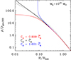 |
Fig. B.1. Gas density profiles derived by solving for hydrostatic equilibrium for 3 different values of Cg as detailed in the label. The dashed gray line shows the distribution of the gas as it is deposited in the gravitational well, without any redistribution. |
As previously pointed out, the system is solved going inwards. Since gas at smaller radii is shock heated before gas at larger radii, in a sense, we solve the system by going back in time. In other words, our scheme allows us to derive numerical solutions, which are not necessarily physical ones. This point is better understood by looking at Fig. B.1, where we show 3 different density profiles derived by solving for 3 distinct values of Cg that differ from one another by ∼0.1%. The gas distribution derived from the  case (black solid line) differs by less than 10% over most of the radial range with respect to the distribution obtained by assuming the gas does not move from the position it is deposited in from the accretion process (gray dashed line). From Eq. B.22 we see that, for
  gas density will increase more rapidly as we go inwards with respect to the
  . This effectively leads to gas being relocated to slightly larger radii, such a process cannot continue indefinitely because, sooner or later, we run out of gas. In the case reported here, where the variation in Cg is modest, the run away occurs at relatively small radii, for larger values of Cg it is located at larger radii. Clearly this is an unphysical solution, and we do not consider it further. The
  is more interesting, here Eq. B.22 leads to a redistribution of the gas from larger to smaller radii. This is a mathematically viable solution, however from a physical point of view things are different.
The broad agreement observed at large radii between entropy predicted under the assumption of full conversion of kinetic into thermal energy and the observed one (see Fig. 6) tells us that the redistribution, that follows the initial deposition of the gas and which is required to reach hydrostatic equilibrium, must be quite modest. This is consistent with findings based on our analysis, in Fig. B.1 we see that, as we move away from the virial/shock radius, Rv ∼ 2.1R500, the density derived by imposing hydrostatic equilibrium remains close to the one derived by simply requiring that the gas remain where it is deposited by the accretion process over a large radial range. In summary we may say that, as the halo grows in size, a redistribution process sweeps outwards in the wake of the expanding accretion shock, leaving behind it a gas distribution which is in hydrostatic equilibrium and close to the one derived by assuming the gas remains where it is deposited by the accretion process. This line of reasoning strongly suggests that the favored solution is the one with  .
.
We implement this solution in our numerical code through a recursive process that solves Eqs. B.21, B.22 and B.23 starting from the value of Cg derived from Eq. B.19. We then compare the density at 0.03 R500 with the one derived assuming gas does not move from where it is deposited by the accretion process and modify Cg to reduce the difference. We iterate until the difference in density at 0.03 R500 is smaller than 10%. The search for  is carried out through a standard bisection method.
Appendix C: A derivation of the temperature correction
In this appendix we derive Eq. 21 presented in Sect. 6.1.1. We start by writing the gas mass falling onto the halo in a time interval Δt,  , as the sum of the masses of the infalling sub-halos:
where dN/dMh is the halo mass function,  is the minimum mass over which the sum is extended and Mh* is the mass of the halo on which the gas is accreting. We note that this description of the process holds as long the timescale over which the halo mass function varies is much longer then Δt, the timescale over which thermalization occurs. The gravitational energy converted into thermal energy through shock heating in the same time interval may be written as
By substituting Eq. C.1 into Eq. C.2, we get
The binding energy of the gas in the potential wells of the sub-halos falling onto the main halo in the time interval Δt, can be expressed as
where Eb(Mh) is the binding energy of the gas within sub-halos of mass Mh. We recall that accreting gas with no energy at infinity, once settled into hydrostatic equilibrium, has a binding energy that equals its thermal energy (Binney & Tremaine 1987).
Thus the binding energy of the gas in a sub-halo of mass Mh can be expressed as the product of the number of gas particles multiplied by the temperature:
Plugging Eq. C.5 into Eq. C.4, we get
The next step is to compute the fraction of the energy made available by gravitational collapse that goes into unbinding the gas from sub-halos. This is
where we have made use of expressions for  and Eth(Mh*) provided respectively in Eqs. C.6 and C.3 and have substituted Mg(Mh) with fg(Mh) Mh. We rewrite T(Mh) as
where Mh, o is a reference halo mass and T(Mh, o) the value temperature takes on at Mh, o. We change the integration variable from Mh to mh = Mh/Mh, o, and with some algebra get
The energy left for the thermalization of the gas is:  . Thus, if we define as mixed accretion temperature, Tma, the gas temperature computed accounting for the energy invested in unbinding gas from infalling sub-halos, we find
where T(Mh*) is the temperature computed assuming all gas is outside infalling sub-halos. In Fig. C.1 we show Tma/T as a function of halo mass.
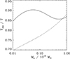 |
Fig. C.1. Mixed accretion temperature, see text for definition, divided by temperature computed assuming all gas is outside infalling sub-halos. The thick line shows the case of a gas fraction that varies with halo mass as in Fig. 8. The dashed line shows the case of a gas fraction that does not depend on halo mass. |
Appendix D: A derivation of the total gas energy
In this appendix we derive the expression for the thermal energy of the gas presented in Eq. 23. In general terms, the thermal energy within a given volume, V, can be written as
where h, is the specific enthalpy (enthalpy per unit mass) and ρg is the gas mass density. Under the standard assumption that gas in the halo can be described as an ideal monoatomic gas:

By assuming spherical symmetry and expressing the product of temperature with density as pressure we rewrite D.1 as
Next, we rescale pressure in units of p500 and radius in units of R500:

where: p500 is the characteristic pressure (see Arnaud et al. 2010, for a definition), V500 = 4/3πR5003, x = R/R500 and p(x) = p(x)/p500. We note also that within the integral we used the symbol x rather than x to avoid confusion with the upper integration limit.
All Figures
|
Fig. 1. Scaled entropy versus halo mass relation for three halos of 1013 M⊙, 1014 M⊙, and 1015 M⊙ at z = 0, respectively. |
| In the text | |
|
Fig. 2. Specific accretion rate versus halo mass relation for three halos of 1013 M⊙, 1014 M⊙, and 1015 M⊙ at z = 0, respectively. |
| In the text | |
|
Fig. 3. Logarithmic slope, dlnKv/dlnMh, versus halo mass relation for three halos of 1013 M⊙, 1014 M⊙, and 1015 M⊙ at z = 0, respectively, as estimated from Eq. (11). Dashed lines were computed neglecting the dlnα/dlnMh term. |
| In the text | |
|
Fig. 4. Logarithmic slope of the radial entropy profile for three halos of 1013 M⊙, 1014 M⊙, and 1015 M⊙ at z = 0, respectively, as estimated from Eq. (15). The radial coordinate has been normalized to the virial radius. |
| In the text | |
|
Fig. 5. Predicted entropy profile for a halo mass of 1013 M⊙ (left panel), 1014 M⊙ (central panel), and 1015 M⊙ (right panel). The radius has been normalized to the shock (virial) radius. All profiles are normalized at the shock radius. In red we plot a reference powerlaw with slope 1.2, in blue the profile derived from a combination of the functional forms: K(R) = Kv(Mh(R)) and in black the one derived by solving the hydrostatic equilibrium equation. |
| In the text | |
|
Fig. 6. Predicted entropy profiles for a halo mass of 1013 M⊙ (blue), 1014 M⊙ (red) and 1015 M⊙ (black) respectively, compared with the observed mean entropy profile and intrinsic scatter (orange shaded region) from the REXCESS sample of galaxy clusters, (Pratt et al. 2010), which features a median mass of M500 ∼ 2.5 × 10¹⁴ M⊙. To ease comparison with observational data, the predicted entropy has been rescaled by K500 and radius by R500. |
| In the text | |
|
Fig. 7. Predicted entropy profiles for a halo mass of 1013 M⊙ (blue), 1014 M⊙ (red), and 1015 M⊙ (black). Dashed lines show entropy from gravitational processes only, solid lines include the effects of pre-heating. The mean entropy profile and intrinsic scatter from the REXCESS sample of galaxy clusters, (Pratt et al. 2010), which features a median mass of M500 ∼ 2.5 × 10¹⁴ M⊙, is reported as an orange shaded region. The region between the 1014 M⊙ and 1015 M⊙ profiles is shown as a gray shaded region. |
| In the text | |
|
Fig. 8. Gas fraction, fg, shown in red and gas mass, Mg, shown in black, as a function of halo mass. The dashed lines show the case where fg = fb and Mg = fbMh at all halo masses. The solid lines show the case modeled by Eq. (18) with parameters chosen as follows: lm = 13, ln = −1, and lσ = 0.6. |
| In the text | |
|
Fig. 9. Gas accretion rate versus halo mass relation for a halo of 1015 M⊙ at z = 0. The blue and red lines have been computed assuming fg follows respectively Eq. (18) and fg = fb. |
| In the text | |
|
Fig. 10. Rescaled entropy versus halo mass relation for four halos of 3 ⋅ 1013 M⊙, 1014 M⊙, 3 ⋅ 1014 M⊙, and 1015 M⊙ at z = 0 respectively. Filled lines have been computed assuming fg follows Eq. (18), dashed ones assuming fg = fb. We note how baryon decoupling produces a break in self-similarity. The change in slope observed at small Mh/Mh, o values for the 3 ⋅ 1013 M⊙ and 1014 M⊙ at z = 0 halos is associated to the minimum in |
| In the text | |
|
Fig. 11.
|
| In the text | |
|
Fig. 12. Halo mass and gas fraction scaled entropy as a function of halo mass for four halos of 3 ⋅ 1013 M⊙, 1014 M⊙, 3 ⋅ 1014 M⊙, and 1015 M⊙ at z = 0, respectively. |
| In the text | |
|
Fig. 13. Radial entropy profiles derived by imposing hydrostatic equilibrium for a halo mass of 1013 M⊙ (blue), 1014 M⊙ (red) and 1015 M⊙ (black) respectively. The radius has been normalized to R500 and the entropy to K500. Filled lines have been computed with baryon decoupling, dashed ones without. |
| In the text | |
|
Fig. 14. Relationship tree connecting the models explored in this paper. The numbers in red at the left of the model name identify the section where the model is discussed. |
| In the text | |
|
Fig. 15. Entropy profiles derived by imposing hydrostatic equilibrium for a halo mass of 1013 M⊙ (blue), 1014 M⊙ (red), and 1015 M⊙ (black), respectively. The radius has been normalized to R500 and the entropy to K500. Filled lines have been computed with baryon decoupling and pre-heating, dashed lines with baryon decoupling and no preheating, dotted lines without either. |
| In the text | |
|
Fig. 16. Radial entropy profiles for a halo of 1015 M⊙ at z = 0. The black filled line shows the profile in the case of single shock at the virial radius. The blue filled line shows a profile modified with a sigmoid of the from reported in Eq. (22) and parameters shown in the figure. The vertical dotted and dashed lines mark the position of R500 and R200 respectively. The slope of the profiles can be gauged by comparison with the power laws plotted as dashed lines. |
| In the text | |
|
Fig. 17. Radial entropy profiles for a halo of 1015 M⊙ at z = 0. The black filled line shows the profile in the case of single shock at the virial radius. The blue filled line shows a profile modified with a sigmoid of the from reported in Eq. (22) and parameters shown in the figure. The vertical dotted and dashed lines mark the position of R500 and R200 respectively. The slope of the profiles can be gauged by comparison with the power laws plotted as dashed lines. |
| In the text | |
|
Fig. 18. Left panel: Entropy in units of K500 versus radius in units of R500. The three blue lines are derived from the model presented in Sect. 5 with corrections described in Sects. 6.1.1 and 6.1.2. All 3 profiles are computed assuming M500 = 1015 M⊙ and for the gas fraction parameters: lm = 13.2 and ls = −0.75. The ln parameter is set to −1.1, −0.7 and −0.3 respectively for the top, medium and bottom curves. The region between the top and bottom curves is shaded for radii where the cooling time is longer than the time since the gas was shock heated. The red shaded region is the median entropy and intrinsic scatter from the HIGHMz sample presented in Riva et al. (2024). The black dashed line shows the self-similar approximation introduced in Voit et al. (2005). Right panel: Density in units of ρg, 500 versus radius in units of R500. The three blue lines are derived from the model presented in Sect. 5 with corrections described in Sects. 6.1.1 and 6.1.2 using the same parameters for the gas fraction adopted for the entropy profile presented in the left panel. The region between the top and bottom curves is shaded for radii where the cooling time is longer than the time since the gas was shock heated. The red shaded region is the median and intrinsic scatter derived from the HIGHMz sample. |
| In the text | |
|
Fig. 19. Top panels: Gas density profiles from the model presented in Sect. 5 with corrections described in Sects. 6.1.1 and 6.1.2 for M500 = 2.5 × 10¹⁴ M⊙ (left), M500 = 5.0 × 10¹⁴ M⊙ (center), and M500 = 1015 M⊙ (right) compared with observations from the REXCESS, XCOP, and HIGHMz samples respectively. For further details see the label of Fig. 18. Bottom panels: Same as top panels but for the entropy profiles. |
| In the text | |
|
Fig. 20. Left panels: Density profiles predicted from our model for halo masses of 5.0 × 10¹³ M⊙ (left) and 1014 M⊙ (right), shown as blue shaded regions, compared with observations from the Sun et al. (2009) sample, shown as a red shaded region (for further details, see the label of Fig. 18). Right panels: Same as left panels but for entropy profiles. |
| In the text | |
|
Fig. 21. Left panel: Radial entropy profiles. The blue and brown shaded regions respectively show the model for M500 = 1014 M⊙ and the Sun et al. (2009) profiles, already reported in Fig. 20. The red, green, violet, and cyan shaded regions represent profiles reported in Eckert et al. (2024). Right panel: Same as the left panel but for the gas fraction profiles. The gray shaded region shows the cosmic baryon fraction. |
| In the text | |
|
Fig. 22. Left panel: Radial entropy profiles for the combined sample extracted from the MACSIS and BAHAMAS simulations (Barnes et al. 2017) compared with the one derived from our model for M500 = 2.5 × 10¹⁴ M⊙ and with the observed REXCESS profile. Right panel: Radial entropy profiles from the FLAMINGO simulation for objects in the M500 = 1014 − 1014.5 M⊙ mass bin compared with the one derived from our model for M500 = 2.5 × 10¹⁴ M⊙ and with the observed REXCESS profile. |
| In the text | |
|
Fig. 23. Gas fraction as a function of halo mass. The solid blue lines show the profiles for the three choices of parameters adopted to fit cluster and group thermodynamic profiles. The blue shaded region spans the region between the different profiles. The red shaded region shows the gas fraction derived in Ettori et al. (2023) to minimize scatter in cluster scaling relations. The gray shaded region shows the cosmic baryon fraction. |
| In the text | |
|
Fig. B.1. Gas density profiles derived by solving for hydrostatic equilibrium for 3 different values of Cg as detailed in the label. The dashed gray line shows the distribution of the gas as it is deposited in the gravitational well, without any redistribution. |
| In the text | |
|
Fig. C.1. Mixed accretion temperature, see text for definition, divided by temperature computed assuming all gas is outside infalling sub-halos. The thick line shows the case of a gas fraction that varies with halo mass as in Fig. 8. The dashed line shows the case of a gas fraction that does not depend on halo mass. |
| In the text | |
Current usage metrics show cumulative count of Article Views (full-text article views including HTML views, PDF and ePub downloads, according to the available data) and Abstracts Views on Vision4Press platform.
Data correspond to usage on the plateform after 2015. The current usage metrics is available 48-96 hours after online publication and is updated daily on week days.
Initial download of the metrics may take a while.