| Issue |
A&A
Volume 689, September 2024
|
|
|---|---|---|
| Article Number | A7 | |
| Number of page(s) | 16 | |
| Section | Extragalactic astronomy | |
| DOI | https://doi.org/10.1051/0004-6361/202450442 | |
| Published online | 28 August 2024 | |
Detecting galaxy groups populating the local Universe in the eROSITA era
1
European Southern Observatory, Karl-Schwarzschildstr. 2, 85748 Garching bei München, Germany
2
Excellence Cluster ORIGINS, Boltzmannstr. 2, 85748 Garching bei München, Germany
3
Leibniz-Institut für Astrophysik Potsdam (AIP), An der Sternwarte 16, 14482 Potsdam, Germany
4
Universitäts-Sternwarte, Fakultät für Physik, Ludwig-Maximilians-Universität München, Scheinerstr.1, 81679 München, Germany
5
Max-Planck-Institut für Astrophysik, Karl-Schwarzschildstr. 1, 85741 Garching bei München, Germany
6
INAF – Osservatorio Astronomico di Trieste, Via Tiepolo 11, 34143 Trieste, Italy
7
IFPU – Institute for Fundamental Physics of the Universe, Via Beirut 2, 34014 Trieste, Italy
8
Max-Planck-Institut für Extraterrestrische Physik (MPE), Giessenbachstr. 1, 85748 Garching bei München, Germany
9
INAF – Osservatorio Astronomico di Brera, Via E. Bianchi 46, 23807 Merate, LC, Italy
10
International Centre for Radio Astronomy Research, University of Western Australia, M468, 35 Stirling Highway, Perth, WA 6009, Australia
11
ARC Centre of Excellence for All Sky Astrophysics in 3 Dimensions (ASTRO 3D), Australia
12
Department of Astronomy, University of Geneva, Ch. d’Ecogia 16, 1290 Versoix, Switzerland
Received:
19
April
2024
Accepted:
4
June
2024
Context. eROSITA will deliver an unprecedented volume of X-ray survey observations, 20 − 30 times more sensitive than ROSAT in the soft band (0.5 − 2.0 keV) and for the first time imaging in the hard band (2 − 10 keV). The final observed catalogue of sources will include galaxy clusters and groups along with obscured and unobscured (active galactic nuclei) AGNs. This calls for a powerful theoretical effort to mitigate potential systematics and biases that may influence the data analysis.
Aims. We investigate the detection technique and selection biases in the galaxy group and AGN populations within a simulated X-ray observation conducted at the depth equivalent to a four-year eROSITA survey (eRASS:4).
Methods. We generate a mock observation spanning 30 × 30 deg2 based on the cosmological hydrodynamical simulation Magneticum Pathfinder from z = 0 up to redshift z = 0.2, mirroring the depth of eRASS:4 (with an average exposure of ∼600 s). We combined a physical background from the real eFEDS background analysis with realistic simulations of X-ray emission for the hot gas, AGNs, and XRB. Using a detection method similar to that utilised for eRASS data, we assessed completeness and contamination levels to reconstruct the luminosity functions for both extended and point sources within the catalogue.
Results. We define the completeness of extended detections as a function of the input X-ray flux S500 and halo mass M500 at the depth of eRASS:4. Notably, we fully recovered the brightest (most massive) galaxy clusters and AGNs. However, a significant fraction of galaxy groups (M200 < 1014 M⊙) remain undetected. Examining gas properties between the detected and undetected galaxy groups at a fixed halo mass, we observe that the detected population typically displays higher X-ray brightness compared to the undetected counterpart. Furthermore, we establish that X-ray luminosity primarily correlates with the hot gas fraction, rather than temperature or metallicity. Our simulation suggests a systematic selection bias in current surveys, leading to X-ray catalogues predominantly composed of the lowest-entropy, gas-richest, and highest surface brightness halos on galaxy group scales.
Key words: methods: data analysis / galaxies: active / galaxies: groups: general / X-rays: galaxies: clusters / X-rays: general
© The Authors 2024
 Open Access article, published by EDP Sciences, under the terms of the Creative Commons Attribution License (https://creativecommons.org/licenses/by/4.0), which permits unrestricted use, distribution, and reproduction in any medium, provided the original work is properly cited.
This article is published in open access under the Subscribe to Open model. Subscribe to A&A to support open access publication.
1. Introduction
Despite their abundance in the Universe (Tinker et al. 2008), the study of galaxy groups (M2001 ∼ 1012.5 − 1014 M⊙) has only recently become feasible through X-rays observations. Their shallow potential wells and faint X-ray emissions pose several challenges in detecting these systems, despite hosting a large fraction of the baryonic mass (Eckert et al. 2021). In contrast to hot galaxy clusters, groups present environments where the baryon physics – cooling, galactic winds, and active galactic nuclei (AGN) feedback – begins to dominate (Eckert et al. 2021). They are not merely scaled-down versions of massive clusters; recent studies have demonstrated the inadequacy of many scaling relations across different mass scales (see discussion in Lovisari et al. 2021; Oppenheimer et al. 2021). The IntraGroup Medium (IGrM) primarily emits through bremsstrahlung interactions, however, cooling through line emission is significant leading to the presence of multi-phase gas in the same environment (e.g. ZuHone et al. 2023). Consequently, X-ray observations serve as a valuable tool for tracing the IGrM and gaining insight into the thermodynamic properties of the hot gas (see Voit et al. 2017; Lovisari et al. 2021, for a review). However, the low surface brightness of these systems can lead to misclassification as pointed emission, necessitating multi-wavelength follow-up observations to resolve such features (Salvato et al. 2022; Bulbul et al. 2022).
In this context, the extended ROentgen Survey with an Imaging Telescope Array (eROSITA) on board the Spectrum-Roentgen-Gamma (SRG) stands as a significant enhancement. eROSITA promises to deliver the first comprehensive census of the entire X-ray sky, boasting high sensitivity in the soft X-ray band and employing a scanning observing strategy (Merloni et al. 2012; Sunyaev et al. 2021). This instrument will overcome previous limitations in statistics, depth, and spatial resolution, allowing us to increase the volume of our X-ray surveys by at least one order of magnitude in the groups and clusters regime and to detect a total of three million AGNs caught at different evolutionary phases and clustering up to z = 2 (Merloni et al. 2012). Its scientific goals range from understanding purely astrophysical phenomena (e.g. characterising the thermal structure and chemical enrichment of halos as a function of redshift) to providing constraints on cosmological parameters (Ghirardini et al. 2024; Artis et al. 2024). These tasks have already shown promising results with the preliminary results from the German sky data releases of the eROSITA Final Equatorial Depth Survey (eFEDS; Brunner et al. 2022) and eROSITA All-Sky Survey-1 (eRASS1; Merloni et al. 2024). eROSITA will deliver the first large statistical determination of cross-correlations between AGNs and clusters or AGNs and groups (Cappelluti et al. 2007), making it key to understanding the interplay between AGN feedback and the hot gas permeating the group environment (e.g. Bahar et al. 2022, 2024).
This challenging endeavour calls for a joint effort on both the theoretical and observational sides to address systematic issues and limitations in our observations. Establishing clear selection functions and understanding potential contamination from background and foreground sources are crucial initial steps. Clerc et al. (2018, 2024), Comparat et al. (2020), Liu et al. (2022a), Seppi et al. (2022) address the issue with a full-sky dark matter (DM) only lightcone on which they paint galaxy properties and X-ray emission based on the most recent observational data. This allowed them to infer the expected X-ray selection function at different exposure times. Nevertheless, these studies lack a self-consistent modelling of the baryon physics in the galaxy population with the environment (Comparat et al. 2020).
From the hydrodynamical simulations side, there have been several efforts to provide predictions for the hydrostatic mass bias (Scheck et al. 2023), projection effects (ZuHone et al. 2023), and gas properties observed in nearby clusters (Biffi et al. 2022; Churazov et al. 2023). However, we still lack a comprehensive study on the halo population and the systematics causing many of these objects to remain undetected (Popesso et al. 2024). Many of these cosmological simulations rely on different feedback prescriptions (Hirschmann et al. 2014; Vogelsberger et al. 2014; Steinborn et al. 2015; Schaye et al. 2015; Davé et al. 2019; Zinger et al. 2020) which are expected to be most effective at these scales (Fabian 2012; Gaspari et al. 2020; Eckert et al. 2021). Comparing the observational data with the simulations will provide the necessary tools to constrain our models. The state-of-the-art simulation Magneticum is a suitable choice to address the task. Unlike other cosmological simulations (e.g. SIMBA, Eagle, and IllustrisTNG Habouzit et al. 2021), Magneticum reproduces the AGN luminosity function well down to z = 2 (Hirschmann et al. 2014; Steinborn et al. 2018; Biffi et al. 2018), which is responsible for most of the X-ray cosmic background, and recovers several scaling relations obtained with eROSITA at the group and galaxy mass scales (Bahar et al. 2022; Zhang et al. 2024). Magneticum achieves this without an explicit calibration on observed scaling relations down to the group-scale halos, in contrast to other state-of-the-art simulations, such as the IllustrisTNG project (Pillepich et al. 2018; Nelson et al. 2018), SIMBA (Davé et al. 2019), and FLAMINGO (Schaye et al. 2023). Thus, we argue that the Magneticum suite is an excellent tool to infer predictions of the hot gas in galaxy groups and investigate the detectability of such objects.
This paper initiates a series of works focussed on testing this framework with a particular focus on the galaxy group regime in the local Universe. We carried out eROSITA mock observations of a patch of the sky (30 × 30 deg2) up to redshift z = 0.2 using the scanning strategy designed for eRASS:4. We reconstructed the selection functions and paved the way for a series of works focussed on the comparison between simulations and observations. Future papers will involve the analysis at higher redshifts for which we create eight lightcones down to z = 1.1 but with a smaller sky area (i.e. 5 × 5 deg2).
The paper is structured as follows. In Sect. 2 we present the set of simulations and the lightcone designed for this experiment. Sect. 3 describes the spectral modelling of the X-ray emission along with the techniques applied to obtain a mock catalogue. Sect. 4 illustrates the matching technique to recover the detected and undetected underlying halo population in the simulations, this will pose the necessary base to reconstruct the selection function. The detected population was used to reconstruct the luminosity function to compare it with the eFEDS luminosity function in Sect. 5. Sect. 6 elaborates more on the selection effects in place which lead to the detection and non-detection of galaxy groups (at a fixed halo mass). Finally, Sect. 7 concludes our study, providing a summary of our findings.
2. Simulations
2.1. The Magneticum simulation
The Magneticum Pathfinder simulation2 is a large set of state-of-art cosmological hydrodynamical simulations carried out with P-GADGET3, an updated version of the public GADGET-2 code (Springel 2005). The most important changes comprehend a higher-order kernel function, time-dependent artificial viscosity, and artificial conduction schemes (Dolag et al. 2005; Beck et al. 2016).
These simulations incorporate several subgrid models to capture the unresolved baryonic physics, including radiative cooling (Wiersma et al. 2009), a uniform time-dependent UV background (Haardt & Madau 2001), star formation and stellar feedback (i.e. galactic winds; Springel & Hernquist 2003), and explicit chemical enrichment (tracing H, He, C, N, O, Ne, Mg, Si, S, Ca, Fe) from stellar evolution (Tornatore et al. 2007). Additionally, they include models for supermassive black hole (SMBH) growth, accretion, and AGN feedback following prescribed methods Springel (2005), Di Matteo et al. (2005), Fabjan et al. (2010), Hirschmann et al. (2014).
Identifying halos and substructures post-simulation involves a two-step process utilising a Friend-of-Friend (FOF) algorithm followed by SubFind (Springel et al. 2001; Dolag et al. 2009).
Many studies have already demonstrated the capabilities and quality of the predictions of Magneticum when compared to the observational data. Without the intent to be comprehensive, we list here the comparison with galaxy properties (Teklu et al. 2015, 2016, 2017; Remus et al. 2017; Schulze et al. 2017, 2018, 2020), galaxy clusters (Biffi et al. 2013; Dolag et al. 2017; Ragagnin et al. 2022), and X-ray emission of galaxies and galaxy clusters (Biffi et al. 2013, 2022; Veronica et al. 2022, 2024; Seppi et al. 2023; Scheck et al. 2023; Vladutescu-Zopp et al. 2023; Bogdan et al. 2023; ZuHone et al. 2023; Churazov et al. 2023; Bahar et al. 2024). Therefore in this work, we use Box2/hr which follows the evolution of a large (352 h−3 cMpc3) cosmological box with 2 × 15843 particles at the following resolutions: mDM = 6.9 × 10⁸ h−1 M⊙ and mgas = 1.4 × 10⁸ h−1 M⊙. The Plummer equivalent length for the DM particles corresponds to ϵ = 3.75 h−1 kpc, whereas gas, stars and black hole (BH) particles retain ϵ = 3.75 h−1 kpc, 2 h−1 kpc and 2 h−1 kpc at z = 0, respectively. The simulation is run with the cosmology from WMAP7 measurements (Komatsu 2010) ΩM = 0.272, Ωb = 0.0168, ns = 0.963, σ8 = 0.809 and H0 = 100 h km s−1 Mpc−1 with h = 0.704.
2.2. Designing the lightcone
The lightcone is designed by extracting random sub-cubes from five different simulation snapshots and arranging them according to our preferred geometrical configuration progressing from the most recent to the furthest. Each sub-cube provides continuity in both angular aperture and depth. This design introduces two primary obstacles to our ability to generate an arbitrary number of lightcones from the same simulation.
Firstly, the choice of depth in redshift z and angular aperture θ of the lightcone are intertwined and limited by the volume of the cosmological box (i.e. a cube of size LBox, thus volume  ). The maximum angular aperture (θmax) permitted is dictated by the geometrical distribution of the sub-cubes and can be expressed as:
Here, w(z, x) denotes the angular distance at redshift z in a universe with cosmological parameters x.
Secondly, the number of independent realisations from a single box is finite and hinges on both the specified geometric configuration (i.e. the maximum sub-cube size Lmax) and the total volume of the box. It can be quantified as,
Given these constraints, we opt to extract a single lightcone measuring 30 deg in both angular dimensions (LC30). In each sub-cube, the particles (and accordingly, the halos and galaxies) are redshifted or blueshifted according to the nominal distance from the observer located at (0, 0, 0). For each halo, we compute the corresponding sky (angular) coordinate in the equatorial system – centred on (RA, Dec) = (0,0) – along with the true and the observed redshifts deduced by the peculiar velocity of the galaxies. This approach facilitates our analysis in redshift-space, where the galaxy distribution is distorted by the finger-of-God effect (Zehavi et al. 2002).
This is not the first time lightcones were generated from the Magneticum output: Dolag et al. (2016) investigated the thermal and kinetic Sunyaev-Zeldovich effect and the mean Compton Y parameter in comparison with the Planck, South Pole Telescope (SPT), and the Atacama Cosmology Telescope (ACT) data.
3. Mock X-ray observation
In this section, we outline the steps for generating the eROSITA mock observation based on Magneticum. These involve the following steps:
-
The lightcones are processed through PHOX (Biffi et al. 2012, 2013, 2018) to produce an ideal event list based on the physical properties of the gas, BH, and stellar particles within the simulation (see Sect. 3.1).
-
The event file is run by SIXTE (Dauser et al. 2019) to extract a mock observation in scanning mode as eFEDS and eRASS:4 (see Sect. 3.2).
-
The resulting mock observation, including all eROSITA instrumental effects and calibrations, are processed with eROSITA Science Analysis Software System (eSASS) to extract extended and point source detections as done in Merloni et al. (2024), Bulbul et al. (2024) (see Sect. 3.3).
A more in-depth description of each stage is given in the following.
3.1. Generating the event file with PHOX
The eROSITA X-ray emission is obtained by modelling the hot gas, AGNs, and X-ray binaries (XRB) in the simulations.
Initially, we generate a photon list using PHOX (Biffi et al. 2012, 2013). The code computes X-ray spectral emission for the aforementioned components based on the physical properties of the gas, BH, and stellar particles in the simulation. A fiducial collecting area Afid and exposure time τfid are initially assumed to sample a discrete and ideally large number of photons from the spectra in a Monte Carlo approach. In the second step, PHOX considers the lightcone’s geometry and projects the emission along the line of sight while photon energies are corrected for the Doppler shift (see Unit2 in Biffi et al. 2018). This second unit follows the prescription derived from the lightcone geometry (e.g. the field of view, and position in the cosmological box) to be consistent throughout. Each component has a different spectral emission modelled with the XSPEC library (v12; Arnaud 1996).
Modelling the hot gas emission. The hot gas emission is assumed to follow vapec (Smith et al. 2001) with a single temperature model and in the presence of heavy elements, for which single abundances are explicitly tracked. Solar abundances are assumed following Anders & Grevesse (1989). The parameters are derived from the chemical and thermal properties of the single gas particles in the simulations. A simple foreground absorber is assumed with the wabs model (Morrison & McCammon 1983) with column density NH = 1020 cm−2. In Fig. 1, we show two scaling relations obtained from the IGrM photons compared to several observational best-fit relations, namely Lovisari et al. (2015), Eckmiller et al. (2011), Arnaud et al. (2010). We calculate these quantities within a spherical aperture with radius R500 centred on the particle at the minimum of the gravitational potential. We refer to Biffi et al. (2012, 2013) for further details on the modelling.
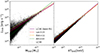 |
Fig. 1. X-ray scaling relations recovered from the halo population in the lightcone: with L500 − M500 in the left panel and L500 − kT500 in the right panel. The luminosity L500 is intended as the IGrM-only emission including Galactic absorption in the 0.1 − 2.4 keV band within R500. For reference, also literature values are reported: Lov+15 (Lovisari et al. 2015), Eck+11 (Eckmiller et al. 2011), Arn+10 (Arnaud et al. 2010). The masses and mass-weighted temperature are calculated in the same radius R500. Considering the small redshift range, we neglect any evolutionary changes in the scaling. |
Modelling the AGN emission. The synthetic X-ray spectrum of AGNs is modelled in PHOX from the properties of BH particles in the simulation with an intrinsically absorbed power-law, having assigned an obscuring torus to every source. The absorber’s column density is randomly drawn from the distribution described in Buchner et al. (2014). More details on the implementation can be found in Biffi et al. (2018). Since then, the absorption model has changed to the tbabs photoionisation cross sections (Wilms et al. 2000), instead of the wabs cross sections (Morrison & McCammon 1983).
Modelling the XRB emission. The emission of XRBs in PHOX, which is stellar in origin, is traced with the star particles in the simulation. The spectral shape is an absorbed (ztbabs) power-law (zpowerlw) with a photon index extracted according to the XRB type. The XRBs can be classified according to the predominant accretion process: wind-fed in the case of high-mass XRBs and Roche-lobe mass transfer in the case of low-mass XRBs. The HMXB has photon index Γ = 2 (Mineo et al. 2012) and the LMXB has Γ = 1.7 (Lehmer et al. 2019). The full description of the XRB emission modelling in PHOX is presented in Vladutescu-Zopp et al. (2023).
3.2. Event files
The synthetic photon lists serve as the input files to the Simulation of X-ray Telescopes (SIXTE) software package (Dauser et al. 2019, v2.7.2), the official eROSITA end-to-end simulator. SIXTE traces the photons through the optics, using the measured point spread function (PSF) and vignetting curves (Predehl et al. 2021) onto the detector. The input ideal photon list is convolved with the redistribution matrix file (RMF) and auxiliary response file (ARF) of the instrument. All seven telescope modules (TMs) use the same RMF and a low-energy threshold of 60 eV. The detection process incorporates a detailed model of the charge cloud and read-out process. The software allows the independent processing of all seven TMs: five of these (TMs 1, 2, 3, 4, and 6) have identical effective area curves, and TMs 5 and 7 have identical effective area curves, due to the absence of the aluminium on-chip optical light filter (Predehl et al. 2021). SIXTE can model the eROSITA’s unvignetted background component due to high energy particles (hitting the camera and generating secondary X-ray emission) and electronic noise (Liu et al. 2022a). We perform mock observations of eRASS:4 (in scanning mode) using the theoretical attitude file for the three components separately and then combine the event files.
We need to include a physical background to LC30, given that the included physics is limited within z < 0.2 and the X-ray cosmic background is dominated by the AGN population (Haardt & Madau 2001; Gilli et al. 2007). A realistic representation can be modelled with the deep background modelling extracted within the eFEDS area (see Liu et al. 2022b). The eROSITA background has been found to be relatively constant in time (Predehl et al. 2021; Brunner et al. 2022; Yeung et al. 2023) and volume (Liu et al. 2022a), we model the physical background as one single extended source with a flat surface brightness. In LC30, the simulated background in all seven TMs is taken from Liu et al. (2022a) and represents the spectral emission from all the unresolved sources in the eFEDS catalogue.
Fig. 2 illustrates the resulting mock X-ray field of view (FOV) with the eSASS detections (see next section). The full emission is included (i.e. IGrM, AGN, XRB, and background). Additionally, we report for comparison the eFEDS’FOV with an orange rectangle in the top-left corner of the image. We zoom in over one of the largest systems at the lowest redshift.
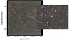 |
Fig. 2. Sky view of LC30 including all the X-ray sources modelled (i.e. IGrM, AGNs, XRBs, and background) with a zoom-in over one of the largest clusters and surrounding environment at the lowest snapshot. We report in red the extended detections and with yellow squares the point-source detections. The circles mark the extension of the source being R200 from the matched input catalogue. The orange rectangle at the top left shows the size of FOV for the eFEDS catalogue (i.e. 140 deg2). |
3.3. eSASS source detection
The reduction of the simulated eROSITA data in this study mirrors the data flow of the eRASS data reduction described in Merloni et al. (2024).
The event files from all emission components and eROSITA TMs are merged and filtered for photon energies within the 0.2 − 2.3 keV band. The filtered events are binned into images with pixel size 4″ and 3240 × 3240 pixels. These images correspond to overlapping sky tiles with size 3.6 × 3.6 deg2 having a unique area of 3.0 × 3.0 deg2. The LC30 is covered by 122 of the standard eRASS sky tiles.
On each sky tile, the eSASS source detection chain detailed in Brunner et al. (2022) is applied. Based on the attitude file used for the SIXTE simulations, we calculate exposure maps and detection masks for each of the tiles using the eSASS tasks expmap and ermask. The task erbox searches for significant excesses in the images and creates an initial source list. After masking out these initial sources, a background map is iteratively refined using an adaptive smoothing algorithm. This refined background map informs further refinement of the source search by erbox. The final erbox lists and background maps are then passed to the PSF fitting task ermldet. This task models the PSF for each photon event based on its energy and detector position. At the input source positions point source and extended source model are fitted to the data. The resulting source catalogue includes fitting parameters for positions, fluxes, and extent for each source. The calculated likelihood values for detection (ℒDET) and extent (ℒEXT) are inversely related to the probabilities 𝒫 for spurious detection by

See Appendix A in Brunner et al. (2022) for further details. Finally, the ermldet source lists from the non-overlapping 3 × 3 deg2 area of each sky tile are merged into the final source catalogue.
4. The eSASS catalogue
In this section, we present the X-ray catalogue created with the eSASS pipeline on LC30 and the matching procedure. We also discuss the types of detections (primary and secondary), the integrated luminosity and the use of luminosity as mass-proxy through scaling relations.
4.1. Extended sources: Matching with the input catalogue
Similar to eFEDS (Liu et al. 2022c) and eRASS1 (Bulbul et al. 2024) catalogues, we focus on the detections within the soft band (0.2 − 2.3 keV). Out of the total 44 459 detections, approximately 94% are composed of point sources. Fig. 3 illustrates the distribution of the resulting 2674 extended detections (ℒEXT > 0) as a function of the extent ℒEXT and detection likelihoods ℒDET. We colour-code the points according to the corresponding angular extension in the catalogue. It is not surprising that at constant ℒDET, the higher ℒEXT corresponds to the detections with the largest angular extension. In Fig. 3 we also draw the minimum values (red dashed lines) for which ℒDET and ℒEXT will be selected as extended sources (i.e. 1675 candidates) in subsequent analyses.
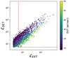 |
Fig. 3. Distribution of the extended ℒEXT and detection likelihoods ℒDET for all the (candidate) extended sources. We colour-coded the points according to their angular scale in arcseconds. The red dashed lines mark the separation between the extent sources above the likelihood we choose to operate (i.e. ℒDET > 5 and ℒEXT > 6). |
The matching procedure goes as follows.
-
For each extended source, we search for a halo counterpart in the Magneticum catalogue which lays within a maximum offset of R500 from the detection’s centre. Being the X-ray emissivity proportional to the electron density square, it is reasonable to direct our matching to the densest regions of the halos.
-
If more than one halo falls within the circular aperture, we check whether there is one whose flux dominates (i.e. at least four times the second brightest source). If this is the case, we match it, otherwise, we define a primary (the brightest detection) and a secondary source not detected due to blending. Even though there might be more than one very bright source in the aperture, we keep track only of the second brightest and flag the primary as blended.
-
At the end, we check whether according to these criteria, any halo in the input catalogue has been matched more than once to an eSASS detection. If so, we define the matched sources as fragmented. Fragmentation occurs in large halos that are split into smaller emissions by eSASS, thus we define the primary detection as the one with the highest flux while the fragments are labelled as secondary.
Thus, according to the likelihood of the matching, we identify two types of detected sources: primary and secondary. Primary detections are either the unique or primary emitting extended source matched. Secondary extended detections are all sources that are impacted by blending or fragmentation. Our reference run is set for ℒDET > 5 and ℒEXT > 6, similarly to the eFEDS catalogue (Brunner et al. 2022). We run the unmatched catalogue through a second matching iteration with the eSASS catalogue of detected point sources (i.e, ℒDET > 5 and ℒEXT = 0) to account for the possibility that a fraction of these halos might be misclassified as point sources due to the sizable PSF of the detector (e.g. Xu et al. 2018; Bulbul et al. 2022). We limit our query to point detections whose flux is dominated (> 50%) by the IGrM photons. Going back to Fig. 2, we illustrate the detections in LC30: the red circles encompass the angular R200 of the source, while the yellow squares correspond to the point-source detections.
4.2. Extended sources: Primary detections
Here, we assess the completeness and contamination of the extended X-ray emissions to understand the detectability of the halo population. Although we perform the matching with the entire halo catalogue, we discuss only the detections corresponding to halos with mass M200 ≥ 1012.5 M⊙ (i.e. due to the simulation’s resolution). Throughout, we use subscripts to denote different categories:
-
“EXT” refers to the extended detection subsample;
-
“HALOS” encompasses all the Magneticum groups and clusters;
-
“SPUR” represents spurious sources (i.e. unmatched detections) in the eSASS catalogue;
-
“eSASS” includes all the detections following the eSASS pipeline.
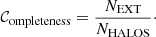
We define completeness as the ratio between the fraction of detected halos to the total number:
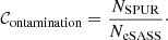
We estimate this quantity (within R500) as a function of the input flux S500 and halo mass M500 in the Magneticum catalogue. Similarly, contamination quantifies the fraction of spurious detections in the eSASS catalogue:
This definition differs from the one provided in Seppi et al. (2022), Liu et al. (2022a) and is equivalent to their spurious fraction. These two quantities are complementary in describing the detection process: completeness defines the accuracy of recovering the input catalogue whereas contamination clarifies to what extent it is susceptible to false detections. Such spurious detections can be due to the (random) background fluctuations that mimic source emission. In Fig. 4 we present the completeness of our X-ray extended catalogue within bins of the input flux within the eROSITA detection band (i.e. 0.2 − 2.3 keV) in the top panel and halo mass in the bottom panel.
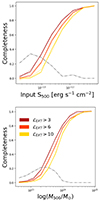 |
Fig. 4. Completeness profiles within the three different extent likelihood cuts (i.e. ℒEXT > 3, 6, 10). The completeness is defined in terms of the input flux S500 in the soft band (0.2 − 2.3 keV) in the top panel and the halo mass M500 in the bottom panel. We present the results for the sample with the extended (primary) detections with the solid lines. The dashed-dotted grey lines show the fraction of misclassified point sources: they are detections from the point source catalogue whose X-ray emission is at least 80% the IGrM in input. The coloured dotted lines are the best-fit curves. |
We perform the matching with the extended catalogue first and, then the point source catalogue (with > 70% emission from IGrM), as outlined in the previous section, however, we vary the cut on the extent likelihood within three values: above 3, 6, and 10. An extent likelihood ℒEXT > 6 is used in constructing the eFEDS catalogue (Liu et al. 2022c), thus it will represent our reference model throughout this analysis. On the other hand, an extent likelihood ℒEXT > 3 is employed for the eRASS1 catalogue (Bulbul et al. 2024) to maximise source discovery. Finally, we include the case for ℒEXT > 10 to check how many of the spurious sources are left out in the process. Not surprisingly, there is a trend of increasing completeness with decreasing ℒEXT threshold: a completeness of 90% is reached at input flux S500 = 1.23 × 10⁻¹² erg s−1 cm−2 (halo mass M500 = 2.1 × 10¹⁴ M⊙) in the ℒEXT > 6 sample. Changing the likelihood threshold allows us to gain only a few per cent on the flux and mass. However, lowering the extent likelihood threshold comes at the expense of the contamination, which increases resulting in 2%, 3%, and 5% for the ℒEXT larger than 10, 6, and 3 respectively. The dotted-dashed grey line represents halos misclassified as point sources due to at least 80% of their X-ray emission coming from the AGNs. Most of these are small halos with a peak at masses around 3 × 10¹³ M⊙. The coloured dotted lines represent the best-fit results for the completeness function and their values are reported in Appendix B. Our baseline model, representing the sample selected with the detection limits adopted for eFEDS (ℒEXT > 6 and ℒDET > 5), will be used throughout the paper.
4.3. Extended sources: Secondary detections
In this section, we discuss secondary sources and their characteristics. Blended and fragmented sources fall in this class. Approximately 5% of the primary detections in the eSASS catalogue (ℒEXT > 6) comprise a second bright source which is not resolved. Liu et al. (2022b) attribute this phenomenon as the primary reason for misclassification in their analysis. Source blending causes a secondary effect on the completeness of the data sample, as the effective observed sources will be reduced. In our case, blended sources impact only mildly the low-mass group regime log(M200/M⊙)∈[12.5, 13.5] an effect that cannot fully account for the drop in the number counts of low-mass systems in Fig. 4.
Very bright and close-up sources may potentially be split into smaller detections by eSASS. We flag as fragmented all sources with more than one counterpart in the eSASS detections. Our analysis reveals fragmentation as the primary source of misclassification, with 12% of matched halos being fragmented into smaller halos by eSASS. Similarly to Seppi et al. (2022), we discover that the fragmentation correlates mostly with the flux of the source, rather than its extension in the sky. In other words, sources with an extended emission will be split into smaller sources preferentially if their input flux is larger than 10−12 erg s−1 cm−2.
In observational analyses, recovering secondary detections poses a significant challenge. Fragmented sources, if discernible into smaller detections, may benefit from optical follow-up and aperture photometry to recalibrate the flux of the extended source. On the other hand, blended sources are confined to be counted as a single source throughout the analysis. Therefore, we decide to further investigate these sources by recalculating the flux within an aperture (see next section) and treating blended sources as a single entity.
4.4. Extended sources: Imaging and luminosity
To mitigate the source fragmentation effect and closely mimic the observational approach, we recompute the rest-frame soft band luminosity of all the extended sources within an aperture equal to R500 of the input halo, rather than relying on the input flux extracted from the Magneticum simulation.
Our imaging analysis is grounded in direct image fitting, involving the deconvolution of the PSF and conversion of the de-projected count rate profile into a surface brightness profile using an energy conversion factor (ECF). The ECF is computed through XSPEC assuming an absorbed apec model with an emission measure of 1. We assume a gas temperature extracted via the M500 − T500 scaling relation in Lovisari et al. (2015) and a fixed metallicity Z = 0.3 Z⊙ (like in PHOX; Anders & Grevesse 1989). We use pyproffit (Eckert et al. 2020) for the task and restrict to the soft energy band (0.5 − 2.0 keV). Images and exposure maps (vignetted and unvignetted) were extracted using the eSASS tools evtool and expmap.
We compare these rest-frame luminosities and their associated errors (16th − 84th percentiles from the MCMC in pyproffit) with the intrinsic luminosity of the sources directly calculated from the mock in Fig. 5. Additionally, we plot in the figure the 1:1 curve in yellow and the running mean in red, to highlight the offset we find between the two estimates. The re-calculated luminosities are mostly consistent with the input luminosities, although slightly underestimated at the high-luminosity end. The scatter in the relation seems to be dependent on the input luminosity, increasing towards fainter halos reaching 20% at maximum in the faintest end. This is not surprising as the recovered luminosities also exhibit larger relative uncertainties. In this regime, the number of events measured in the chosen aperture is largely reduced due to the intrinsic faintness of the IGrM: colder gas, metallicity, and lower gas fractions dramatically impact the X-ray emissivity (Eckert et al. 2021; Oppenheimer et al. 2021).
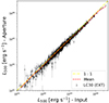 |
Fig. 5. Comparison between the soft band luminosity recovered from the flux aperture in the mock observation and the input luminosity of the halos in the lightcone. The uncertainties are calculated as the 16th and 84th percentile from the MCMC run. We overplot the 1:1 relation in yellow and the best-fit relation in red. |
Additionally, Galactic absorption further damps the emission of such systems. At the high-luminosity end, the impact of assuming a single temperature to estimate to fit the surface brightness profile and constrain the luminosity spans ∼5% (ZuHone et al. 2023), much smaller than the expected statistical uncertainty from the eROSITA observations.
In Fig. 6, we depict the luminosity distribution as a function of the redshift for extended sources. The error bars represent the 16th and 84th percentiles from the Monte Carlo Markov Chain (MCMC) run in pyproffit. We colour-code the points according to their extent likelihood in the eSASS catalogue in arcseconds. Additionally, shaded areas denote the survey flux limit at different completeness rates, ranging from 10% (corresponding to 4.5 × 10⁻¹⁴ erg s−1 cm−2) to 90% (8 × 10⁻¹³ erg s−1 cm−2) in steps of 10%, illustrating the survey’s sensitivity across various luminosity levels and redshifts. Notably, the relation traverses an underdense region between 0.035 ≤ z ≤ 0.05 corresponding to a small void in the lightcone. The red curves represent the flux limits for 40% and 30% completeness for the eFEDS and eRASS1 surveys, respectively.
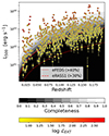 |
Fig. 6. Soft band luminosity distribution of the groups and clusters in the lightcone in function of their redshift. The errors are the 16th and 84th percentile from the MCMC process to extract the luminosity. The data points are colour-coded for their extent likelihood. The shading areas represent the range of survey flux limits given by the completeness from 10% to 90% in steps of 10% difference with decreasing colour. The red curves represent the flux limit in eFEDS (1.5 × 10⁻¹⁴ erg s−1 cm−2; Liu et al. 2022c) and eRASS1 (10−13 erg s−1 cm−2; Seppi et al. 2022) for 40 and 30% completeness respectively. |
4.5. Extended sources: mass recovery
The matching technique allows us to infer the intrinsic properties of the detected and undetected halos and gather information regarding the biases and systematics affecting the detection process (Bulbul et al. 2022; Popesso et al. 2024). Future studies will further elucidate these effects (Toptun et al., in prep.; Dev et al., in prep.). Here, we discuss the consequences of using the estimated intrinsic luminosity to recover the X-ray observables, such as the halo mass M500.
Together with redshift, the halo mass plays a pivotal role in testing models of structure formation and constraining cosmological parameters (Grandis et al. 2019; Pratt et al. 2019). The most common and reliable mass-proxies are calibrated through galaxy kinematics (Pratt et al. 2019), X-ray temperature via hydrostatic equilibrium and weak lensing (Umetsu 2020). When such methods are unavailable, one has to rely on other estimators. Assuming that the hot intracluster medium follows the scale-free gravitational collapse of DM, Kaiser (1986) derive X-ray scaling relations among different thermodynamic properties. The calibration of the X-ray L500 − M500 relation is extensively discussed in the literature highlighting that most findings exhibit slopes from 1.4 to 1.9 steeper due to the presence of non-gravitational processes (Lovisari et al. 2021, for a review).
In our experiment, we calculate the halo masses using the scaling relation derived in Lovisari et al. (2015) which is based on a sample of ∼80 between clusters and groups of galaxies, whose masses have been determined by X-ray data and hydrostatic equilibrium assumption. Our choice stands with the scaling relation used to determine the radius R500 (and thus, the mass M500) in the eFEDS analysis (Liu et al. 2022c) which also results as the closest relation to our best-fit. As a second test, we employ the scaling relation deduced with a subsample from the eFEDS clusters and groups catalogue (Chiu et al. 2022) using weak lensing measurement covered by the Hyper Suprime-Cam (Aihara et al. 2018). Despite no significant difference between the luminosity and temperature of the detected clusters in eRASS1 and eFEDS (Bulbul et al. 2024), some discrepancies have been reported in clusters and groups from eRASS1 between luminosities (eROSITA and Chandra; Bulbul et al. 2024) and temperatures (eROSITA and XMM-Netwon; Migkas et al. 2024) measured with different telescopes. Thus, we expect the scaling relation L500 − M500 derived in Chiu et al. (2022) to differ from others.
Fig. 7 reports our findings. The distribution of points marks the estimated masses for the single halos when applying the scaling relation in Lovisari et al. (2015). This relation is calibrated for an X-ray luminosity in the 0.1 − 2.4 keV energy band, whereas our luminosity is estimated in the band 0.5 − 2.0 keV, therefore we correct the normalisation assuming an ECF of 1.34 (assuming an absorbed apec emission with a mean redshift of 0.1, temperature 1 keV, abundance 0.3 and Galactic absorption with a column density of NH = 1020 cm−2). Furthermore, we check with the input luminosity in this band the accuracy of such prescription and the lack of systematics at this stage. In dash-dotted yellow, we overplot the 1:1 relation to compare the dashed red, namely the best-fit of the points shown – whose masses are calculated with Lovisari et al. (2015) – and the dotted blue corresponding to the best-fit of the points (not shown) whose masses are calibrated with Chiu et al. (2022). Although we do not discover a constant offset in the mass with the former, we note significant differences in the distribution. At the low-mass end, the distribution presents large relative uncertainties and a large scatter from the 1:1 relation: the scatter in the scaling relation is around ∼20% at fixed mass (Lovisari et al. 2015). On the other hand, the mass estimated with the scaling relation from eFEDS (Chiu et al. 2022) provides masses 20% larger in the whole range, as illustrated by the best fit in the figure. We do not attempt to determine the tilt in the eFEDS sample.
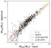 |
Fig. 7. Comparison of the mass distribution in the input catalogue and derived from the scaling relation L500 − M500 in Lovisari et al. (2015). The errors are derived from the 16th and 84th percentile in the luminosity measurement. In dash-dotted yellow, we report the 1:1 relation; in dashed red the best fit from the scatter plot. Additionally, we determine the mass using the scaling relation derived from eFEDS data in Chiu et al. (2022) and plot its best fit as dotted blue. |
Among the many uncertainties on the observational side, we argue that an accurate estimate of the X-ray emission within the halo radius R500 can moderately impact the luminosity, and in turn the scaling relation. In Appendix A, we provide a brief discussion on the impact of the flux estimates when the radius is not properly estimated. In our simulated run, we expect such deviations to happen mostly at the high mass end, where the surface brightness profile is steeper. Furthermore, any deviation from the condition of hydrostatic equilibrium can bias the estimates of cluster masses (Rasia et al. 2006; Nagai et al. 2007; Pratt et al. 2009; Biffi et al. 2016; Gianfagna et al. 2021, 10−20%). Cosmological accretion and turbulent motion (Vazza et al. 2017; Gaspari et al. 2020), viscosity, and thermal conductivity (ZuHone et al. 2015; Gaspari et al. 2015) can all provide such circumstances. Additionally, ZuHone et al. (2023) show that projection effects have a negligible impact.
We argue that the uncertainty in the mass estimation derived from the mass-luminosity scaling relation is unbiased but carries a significant scatter (∼20 − 30%; Lovisari et al. 2015). The possibility of using an alternative mass estimator that exploits the tightness of the mass-temperature relation would considerably decrease the uncertainty (to 8 − 15%; Rasia et al. 2014) even though masses are usually deduced after a single temperature fit to the spectrum which tends to underestimate the masses of 10 − 15% (Rasia et al. 2014).
4.6. Point-sources: Matching and luminosity
Up to this point, we have treated point sources (i.e. ℒEXT = 0) with the sole purpose of re-discovering misclassified halos in the catalogue. In this section, we delve into their presence as pure detections in the eSASS catalogue, since they constitute 86% of all the sources with detection likelihood ℒDET > 10. They are most predominantly composed of bright AGNs (Brandt & Alexander 2015), known to contribute mostly to the cosmic (soft) X-ray background of the Universe (e.g. Schmidt 1968; Gilli et al. 2007).
We select point sources with ℒDET > 10, which should yield a completeness of 94% in an eFEDS-like survey (Liu et al. 2022b). We match these sources to our AGN input catalogue within a distance of 20″ between the detection and the AGN position, similarly to Seppi et al. (2022). We find a completeness of 93% within the flux limit of 1.6 × 10⁻¹⁴ erg s−1 cm−2, in line with the predictions in Merloni et al. (2012). We account for the possibility of blending between point sources, although only 2% of all detections seem to suffer from it.
We extract the rest-frame soft band luminosity directly from the PSF fitting performed by eSASS assuming an ECF between counts and flux in 0.5 − 2.0 keV of 1.604 × 10¹² (erg cm−2)−1 (Brunner et al. 2022). The ECF is calculated assuming an absorbed power-law with Γ = 1.8 and Galactic absorbing column density of NH = 1020 cm−2 which reflects our AGN modelling (Biffi et al. 2018).
5. The X-ray luminosity function
The X-ray luminosity function (XLF) describes the distribution (i.e. number density) of X-ray sources in a survey as a function of their luminosity. A common approach to derive a non-parametric XLF is based on the 1/Vmax technique described in the seminal work by Schmidt (1968) and later generalised by Avni & Bahcall (1980). Hence, the sources are parsed into luminosity bins ΔL such that in the i-th bin the XLF centred on Li is given by:
![$$ \begin{aligned} \frac{\mathrm{d}n}{\mathrm{d}L} (L_i) = \frac{1}{\Delta L_i} \sum _j \frac{1}{V_{\rm max}[L_j, F_{\rm lim}, A(F_j)]}\cdot \end{aligned} $$](/articles/aa/full_html/2024/09/aa50442-24/aa50442-24-eq7.gif)
Here, Vmax is the (shell) comoving volume in which a halo j-th of luminosity Lj in the i-th bin can be detected above the flux limit Flim, considering the sky coverage of the survey A(Fj) (i.e. the FOV of the lightcone: 900 deg2). We estimate Li as the median luminosity of the halos in the bin. This prescription is similar to the one outlined in Liu et al. (2022c) although we omit the selection function term in our calculation.
5.1. Extended detections: Groups and clusters of galaxies
We determine the XLF for the extended (primary) sources in the catalogue and evaluate the differences by including all the X-ray sources in the lightcone. Although eRASS:4 is not a flux-limited survey, we set a flux limit to 1.4 × 10⁻¹³ erg s−1 cm−2 which corresponds to 50% catalogue completeness (see Fig. 6) and determines the upper bound to the redshift integration in the shell volume.
In Fig. 8 we show the lightcone curves in blue: the solid line represents the XLF calculated with input simulation luminosity for all the halos whereas the dotted line is the XLF estimated with the extended (primary) detections corrected for the effective volume. The correction for the effective volume Vmax leads to a mildly steeper XLF than the theoretical one calculated from all the halos. The errors for the XLF given in the figure are the Poisson uncertainties on the number of objects per bin. We plot the XLF estimated using the eFEDS (in orange) and eRASS1 (in green) sample: these curves are normalised for the detection probability as described in Liu et al. (2022c). We remind that both curves are extracted for group and cluster samples up to z = 1.3. We also report findings from the XXL-C1 sample in the [0.01, 0.35] redshift range (Adami et al. 2018) and from the REFLEX II sample (Böhringer et al. 2014) from halos in the local Universe, rescaled to measure luminosities in the 0.5 − 2.0 keV energy range.
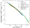 |
Fig. 8. XLF of the intrinsic soft band (0.5 − 2.0 keV) for the extended sources in the lightcone. We plot the results for the full sample (solid blue line) and for only detected ones (dotted blue line). The shaded bands represent the Poisson uncertainty in the luminosity bin. Similarly, we show the XLF for the eFEDS (Liu et al. 2022c) and eRASS1 (Bulbul et al. 2024) data in orange and green respectively. For reference, we also add other results from the literature in black: the XXL-C1 sample (Adami et al. 2018) and the REFLEX II (Böhringer et al. 2014). |
We find relatively good agreement at all luminosities among all sets, except with Adami et al. (2018) at 1043 erg s−1 which also has the largest uncertainties in that range. The lightcone XLFs appear mildly steeper than the observational counterpart, albeit still within 1σ.
5.2. Point source detections: AGNs
We derive the XLF for both detected and undetected AGNs within the lightcone. The validity of the XLF for bolometric luminosity has already been established in the Magneticum boxes across both high (Hirschmann et al. 2014; Steinborn et al. 2015) and low redshifts (Biffi et al. 2018). Here, we assess the XLF in the lightcone regime with Galactic absorption, thus we do not attempt to correct the fluxes to recover the unabsorbed emission.
Fig. 9 illustrates the results in comparison with the XLF extracted from the mock catalogue presented in Marchesi et al. (2020) restricted within a redshift range [0.0, 0.2] and rescaled for our sky area. We report the (intrinsic 0.5 − 2.0 keV) XLF both from our detected population (dotted line) and the total population (solid line) of AGN. We find good agreement in the high luminosity regime (≳5 × 1042 erg s−1), despite an overestimation at intermediate luminosities ∼1043 − 5 × 1043 erg s−1. The set from Marchesi et al. (2020) is complete down to much lower fluxes (5 × 10⁻²⁰ erg s−1 cm−2), which explains the different shapes in the profiles at luminosities < 5 × 1042 erg s−1. Accounting for the effective volume of the survey, allows the XLF for LC30 (PNT) to recover part of the missing population in LC30. Previous works (Hirschmann et al. 2014; Biffi et al. 2018) have already shown the AGN luminosity function in Magneticum in the absence of Galactic absorption.
 |
Fig. 9. XLF of the intrinsic soft band (0.5 − 2.0 keV) for the AGNs in the lightcone. The luminosities are not corrected for Galactic absorption. We report the results for both the detected population (dotted blue line) and the entire population (solid blue line). In orange, we plot the XLF extracted from the mock catalogue in Marchesi et al. (2020) properly rescaled to account for the survey volume difference. The shaded band illustrates the Poisson uncertainty. |
The unresolved faint point sources will constitute part of the physical X-ray background in the mock, predominantly modelled by the real eFEDS background spectrum (see Sect. 3). Another fraction of this background consists of the electronic noise modelled by SIXTE.
6. The hidden bias: Undetected sources
Fig. 4 indicates that for masses below M500 ≤ 1014 M⊙, the eRASS:4 completeness should drop quickly, reaching approximately 50% at 1013.5 M⊙. In this section, we explore with the help of Magneticum which gas properties might be the key driving the observed selection function. This is fundamental to understanding the group population that the eRASS:4 selection function will be capable of detecting, as well as identifying any potential biases. We specifically investigate the role of the electron density, and thus, the hot gas mass fraction, temperature, and metallicity with the halo X-ray emissivity and thus, the detectability through eROSITA.
6.1. Factors influencing X-ray emissivity
Fig. 10 displays the resulting X-ray surface brightness profiles (rest-frame 0.5 − 2.0 keV) from both the extended detections and the undetected population in different halo mass bins (refer to the top of each panel for the corresponding logarithmic M200). Each panel also presents the number of detected and undetected sources within each bin. We only include photons from the IGrM, excluding contributions from background, AGN, and XRB, and omit the inner core of the profiles when the softening length is of similar scales.
 |
Fig. 10. Median X-ray surface brightness of the extended detected (red) and undetected (blue) sources in the 0.5 − 2.0 keV for four different logarithmic halo mass bins (i.e. log(M200/M⊙) reported at the top of each panel). In the lower left of each panel, we report the number of detected and undetected in the mass bin. The shaded bands illustrate the 16th − 84th percentiles from the intrinsic distribution. |
Consistently across all mass bins < 1014 M⊙, we observe a systematic shift in the profiles: the undetected population tends to exhibit lower surface brightness, rendering it more challenging to be detected by eSAS. In the highest-mass bin, the undetected population is composed of halos at the higher redshift (14 out of 21), often close in projection to another (detected) halo (6 out of 21) and with a significant AGN flux (4 out of 21). Hence, the surface brightness profiles of the two populations when stacked almost overlap.
These results are consistent with the studies reported in Popesso et al. (2024), where the authors show the average X-ray surface brightness profiles of the undetected galaxy group population when stacked on the optical peak emission derived from the GAMA survey Driver et al. (2022). Popesso et al. (2024) argue that the undetected population may be the descendant of a post-merger phase, resulting in the observed lower concentration and younger stellar populations. Such events could be associated with the halo’s location in the large-scale structure (e.g. voids, filaments) and/or differences in mass accretion rates.
To investigate the physical reasons behind fainter surface brightness at fixed halo mass, we split the full sample into equally log-spaced bins of halo mass M200 and characterise the X-ray emissivity (i.e. the energy emitted per time and volume), which reads
Here, ne denotes the electron density, and Λν the cooling function at frequency ν both dependent on the gas properties. We investigate the dependence of the scatter of the L500 − M500 relation of Fig. 1 with ne, T, and Z. The scatter is estimated as residuals (ΔL500) with respect to the Lovisari et al. (2015) relation, which best represents the Magneticum data (see Fig. 1). This analysis is conducted within different radii from 0.15 R500 to R500. We restrict to halos with at least 80 particles within the selected sphere to provide a robust statistical measurement and in the halo mass bin 1013 − 1013.5 M⊙. To guide the eye, we also overplot the running median as a function of the scatter with a black line. The most significant dependence is within the system core at 0.15 R500.
Fig. 11 illustrates the residuals ΔL500 versus the three gas properties in a single halo mass bin (i.e. 1013 − 1013.5 M⊙). The same trends are found at all halo masses.
 |
Fig. 11. Properties of the gas as a function of the scatter in the scaling relation L500 − M500 by Lovisari et al. (2015) in one halo mass bin (1013 − 1013.5 M⊙). From the top to bottom panels, we show temperature, metallicity, and gas fraction (all mass-weighted) measured within 0.15 R500 of each halo. The black line denotes the running median for each quantity. We also report the Spearman coefficient in the plot. |
Spearman coefficients for the T, Z, and  are −0.48, 0.15, and 0.60, respectively, indicating that the strongest dependence comes from the electron density. A weak, yet insignificant, anticorrelation is found with the temperature, while there is no discernible dependence from the metallicity. The Spearman coefficient decreases by 35% going from 0.15 R500 to R500, suggesting that the emission from the core region is dominating the emissivity and the system detectability from eROSITA as already suggested in Clerc et al. (2018), Seppi et al. (2022). Lower
  values correspond to lower X-ray luminosities at fixed halo mass, implying a dependence on the hot gas mass fraction, suggesting that halos with low fgas are under-luminous in X-rays at fixed mass.
We generalise this discussion in Fig. 12 which illustrates the effect of the (mass-weighted) hot gas fraction in the X-ray luminosity (0.5 − 2.0 keV) integrated up to R500: lower gas fractions correspond to lower luminosities. Therefore, the faint undetected population likely maintains, on average, lower hot gas fractions than detected halos. These findings, previously discussed in the cluster regime Ragagnin et al. (2022) for the Magneticum simulation, hold in the group regime as well.
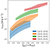 |
Fig. 12. Luminosity of the IGrM as a function of the fraction of hot gas within the same radius (i.e. R500). The halos are binned in logarithmic halo mass M200 (see legend). The shaded bands mark the 68th confidence intervals. |
6.2. The central role of entropy
To further support this argument, we examine the resulting entropy in these systems. The entropy K of the IGrM is defined

where T denotes the temperature of the gas and ne represents the electron density. In Fig. 13, we present the entropy as a function of the scatter ΔL500 revealing that low-entropy systems (i.e. where the gas fraction at the centre is high) have the highest scatter ΔL500. Turning the argument around, we can say that the brightest sources correspond to sources with the lowest entropy intake at the centre. These structural differences highlight a selection effect in our measurements whereby we favour samples at lower entropy (i.e. gas-rich).
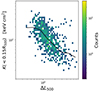 |
Fig. 13. Entropy of the hot IGrM measured within 0.15 R500. We plot it as a function of the scatter in the scaling relation L500 − M500 by Lovisari et al. (2015) in one halo mass bin (1013 − 1013.5 M⊙). |
This intrinsic bias can be highlighted by comparing the recent observational results published in Bahar et al. (2024) with our detected and undetected halos in Fig. 14. Following the approach adopted in Bahar et al. (2024), we calculate the entropy averaged within three different radii (i.e. 0.15 R500, R2500, and R500) to illustrate the impact of the gas phase-space structure at different apertures. We remind Bahar et al. (2024) provides results for the detections from the eRASS1 catalogue, albeit calculating the gas properties with the (deeper) eRASS:4 data. On the other hand, we mock an eRASS:4 lightcone with detections extracted in the eRASS:4 exposure time. This can potentially lead to small differences in the final results. Furthermore, we clarify that although comparable, the profiles we extract for the full sample of halos (represented by the dashed black line) differ from those presented in Bahar et al. (2024). While the authors in that study calculate average electron density and temperature profiles integrated up to the given radius, we compute a single mass-weighted temperature and electron density for each halo. We account for the redshift evolution including the dependence on the self-similar growth parameter E(z) = [ΩM(1 + z)3 + ΩΛ]1/2 in the y-axis. The shaded bands represent the 25th − 75th percentiles from the sample.
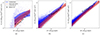 |
Fig. 14. Entropy within different radii as a function of the integrated temperature (within R500). The entropy is calculated for each halo as the ratio between the mass-weighted temperature and the electron density within that same radius. We calculate the running median for the detected (red), undetected (blue), and full sample (black). We plot the 25th − 75th percentiles with the shaded band. The black crosses represent the observational eRASS1 dataset from Bahar et al. (2024). The three images refer to three different radii (i.e. 0.15 R500, R2500, R500). We ensure halos host at least 80 gas particles within the selected aperture. |
Observational data aligns with the predictions from simulations for entropy within R2500 and R500 within the confidence interval. Furthermore, the difference between the detected and undetected population is negligible for most of the temperature range, or at least within the uncertainty, for these radial ranges.
However, a distinct trend emerges for the very inner core (0.15 R500), where the undetected and detected populations seem to diverge with decreasing temperatures (i.e. smaller mass), despite exhibiting significant scatter. Although the detected population remains above the observational data, a much better agreement is observed when considering the potential selection effect due to differences in gas fractions at fixed halo mass.
Considering that the observational data reported in Bahar et al. (2024) refers to detections with exposure time similar to eRASS1, we can expect less bright objects (which we can detect in our configuration) to be undetected in the observational analysis, further lowering the plotted profiles. Moreover, they include a different extent likelihood (i.e. ℒEXT > 3), less conservative than our choice (i.e. ℒEXT > 6). The origins and potential causes for such low gas fractions in the undetected population will be the object of future studies.
7. Summary
eROSITA promises an unparalleled view of the galaxy group mass regime through its X-ray observations, offering insights into the thermodynamic properties of the IGrM and advancing our understanding of baryonic mass in the Universe. To support such observational effort, a direct and meaningful comparison with the state-of-the-art cosmological simulations is necessary to assess and discuss any systematic biases in our investigations.
The results outlined in this study are based on the Magneticum Pathfinder, a publicly available set of cosmological hydrodynamical simulations (Hirschmann et al. 2014), which is used to construct synthetic X-ray observations in a 30 × 30 deg2 lightcone down to redshift z = 0.2. The Magneticum set has proved in previous studies to well-reproduce the observed eROSITA scaling relations at both galaxy and galaxy group’s scales (Bahar et al. 2024; Zhang et al. 2024) and the AGN luminosity function (Biffi et al. 2018), without explicit calibration of the gas properties at these scales.
Our methodology involves extracting X-ray photons using PHOX (Biffi et al. 2012, 2013, 2018; Vladutescu-Zopp et al. 2023) which models the emission from hot gas, AGNs, and XRBs, considering absorption processes and spectral characteristics. Event files are then created with SIXTE (Dauser et al. 2019), a software package simulating the detection process and background components in a mock eROSITA observation with the first four eROSITA all-sky surveys combined (eRASS:4) depth (Predehl et al. 2021). The modelling of foreground and background emissions, including contributions from unresolved sources and Galactic components, is discussed in detail and adapted from the recent observational results (Liu et al. 2022b; Ponti et al. 2023). We run the halo finder eSAS on the event files to reconstruct the extended and point source catalogues in the 0.2 − 2.3 keV band.
Our findings can be summarised as follows:
-
The eSAS detections predominantly comprise point sources (i.e. AGNs, misclassified faint halos, fluctuations in the background) and only 6% of extended sources. Matching according to the spatial distribution and high flux of the extended sources reveals the completeness of the survey as a function of the input flux and mass as shown in Fig. 6. This corresponds to a contamination of 3% in the extended eSAS catalogue. Misclassification of extended-to-point sources is significant at low fluxes (or low mass), as shown in Fig. 4. Blended sources only sum up to 5% (or less including a second match with the point source catalogue) thus it does not represent our largest source of misclassification which is fragmentation (12%) of up-close sources. We find that fragmentation is more prone in high-flux sources (> 10−12 erg s−1 cm−2) rather than extended ones.
-
Luminosities of extended detection are extracted through flux aperture estimation within the input halo R500. We recover unbiased luminosities, despite a mild scatter which increases (reaching ∼20%) towards lower luminosities, as illustrated in Fig. 5. We argue that this regime corresponds to halos with low number counts affecting our spectral reconstruction. Assuming a 50% completeness to determine the selection function returns a survey flux limit of 9.03 × 10⁻¹⁴ erg s−1 cm−2. Fig. 6 shows the outcome of the luminosity versus redshift distribution of the clusters and groups of galaxies.
-
This flux limit is used to derive the non-parametric (and unbiased) XLF in the lightcone comparable to the eFEDS and eRASS1. Fig. 8 presents the final shape of the XLF with some comparisons drawn from the literature in the nearby Universe.
-
We discuss scaling relations to recover the halo mass of the extended detections, providing a 1:1 comparison with the input mass M500 in Fig. 7. We show that deriving halo masses from luminosities can yield large uncertainties due to the large scatter in the scaling relation.
-
In Fig. 9 we present the XLF reconstructed for the detected AGN population compared to the one extracted from the mock catalogue described in Marchesi et al. (2020). Our results show that the bright end of the XLF (> 1043 erg s−1) is fully consistent with these results, whereas for lower luminosities we find some tensions.
-
We discuss the selection effects in an eRASS:4 observation derived from the different gas fractions at fixed halo mass which leaves a significant imprint in the X-ray emissivity (see Figs. 10–14 and discussion there). Such an effect leads to more easily detecting halos with low entropy corresponding to less centrally concentrated and gas-richer systems.
Our study underscores the suitability of eROSITA for detecting galaxy clusters (i.e. M200 > 1014 M⊙) with high completeness and purity, particularly when supplementing the extended detections with matches from the point source catalogue (Bulbul et al. 2022). However, in the group regime, where halo mass decreases, completeness diminishes, necessitating complementary observations across different wavelengths to mitigate Malqumist bias. The detection of galaxy groups is fraught with significant selection effects, biasing samples towards high X-ray luminous halos. Stacking not X-ray selected systems emerges as a viable approach to elucidate the bulk properties of groups, shedding light on the distribution of baryonic mass and its impact on structure formation in a cosmological context (Voit 2005; Eckert et al. 2021). Moreover, understanding the co-evolution of SMBHs with host halos represents a critical aspect of galaxy formation and evolution, influenced by various AGN feedback models implemented in numerical simulations. Moving forward, continued efforts to refine observational techniques and theoretical models will be crucial for unravelling the complex interplay between baryonic processes, structure formation, and the cosmic web, ultimately deepening our insights into the fundamental properties of the Universe.
Acknowledgments
We thank Stefano Marchesi and Roberto Gilli for their help on the AGN cosmic background and Nicola Locatelli for the useful discussion on the Galactic foreground emission. We would also like to show our gratitude to Andrea Biviano for the invaluable comments on the draft. IM and VT acknowledge support from the European Research Council (ERC) under the European Union’s Horizon Europe research and innovation programme ERC CoG (Grant agreement No. 101045437, PI P. Popesso). KD acknowledges support by the COMPLEX project from the ERC under the European Union’s Horizon 2020 research and innovation program grant agreement ERC-2019-AdG 882679. VB and SVZ acknowledge support by the DFG project nr. 415510302. NM acknowledges funding by the European Union through a Marie Skłodowska-Curie Action Postdoctoral Fellowship (Grant Agreement: 101061448, project: MEMORY). YZ and GP acknowledge financial support from the European Research Council (ERC) under the European Union’s Horizon 2020 research and innovation program HotMilk (grant agreement No. 865637). GP acknowledges support from Bando per il Finanziamento della Ricerca Fondamentale 2022 dell’Istituto Nazionale di Astrofisica (INAF): GO Large program and from the Framework per l’Attrazione e il Rafforzamento delle Eccellenze (FARE) per la ricerca in Italia (R20L5S39T9). The calculations for the Magneticum simulations were carried out at the Leibniz Supercomputer Center (LRZ) under project pr83li. E. Bulbul acknowledges financial support from the European Research Council (ERC) Consolidator Grant under the European Union’s Horizon 2020 research and innovation program (grant agreement CoG DarkQuest No 101002585).
References
- Adami, C., Giles, P., Koulouridis, E., et al. 2018, A&A, 620, A5 [NASA ADS] [CrossRef] [EDP Sciences] [Google Scholar]
- Aihara, H., Arimoto, N., Armstrong, R., et al. 2018, PASJ, 70, S4 [NASA ADS] [Google Scholar]
- Anders, E., & Grevesse, N. 1989, Geochim. Cosmochim. Acta, 53, 197 [Google Scholar]
- Arnaud, K. A. 1996, ASP Conf. Ser., 101, 17 [Google Scholar]
- Arnaud, M., Pratt, G. W., Piffaretti, R., et al. 2010, A&A, 517, A92 [CrossRef] [EDP Sciences] [Google Scholar]
- Artis, E., Ghirardini, V., Bulbul, E., et al. 2024, A&A, submitted [arXiv:2402.08459] [Google Scholar]
- Avni, Y., & Bahcall, J. N. 1980, ApJ, 235, 694 [NASA ADS] [CrossRef] [Google Scholar]
- Bahar, Y. E., Bulbul, E., Clerc, N., et al. 2022, A&A, 661, A7 [NASA ADS] [CrossRef] [EDP Sciences] [Google Scholar]
- Bahar, Y. E., Bulbul, E., Ghirardini, V., et al. 2024, A&A, submitted [arXiv:2401.17276] [Google Scholar]
- Beck, A. M., Murante, G., Arth, A., et al. 2016, MNRAS, 455, 2110 [Google Scholar]
- Böhringer, H., Chon, G., & Collins, C. A. 2014, A&A, 570, A31 [NASA ADS] [CrossRef] [EDP Sciences] [Google Scholar]
- Biffi, V., Dolag, K., Böhringer, H., & Lemson, G. 2012, MNRAS, 420, 3545 [NASA ADS] [Google Scholar]
- Biffi, V., Dolag, K., & Böhringer, H. 2013, MNRAS, 428, 1395 [Google Scholar]
- Biffi, V., Borgani, S., Murante, G., et al. 2016, ApJ, 827, 112 [NASA ADS] [CrossRef] [Google Scholar]
- Biffi, V., Dolag, K., & Merloni, A. 2018, MNRAS, 481, 2213 [Google Scholar]
- Biffi, V., Dolag, K., Reiprich, T. H., et al. 2022, A&A, 661, A17 [Google Scholar]
- Bogdan, A., Khabibullin, I., Kovacs, O., et al. 2023, BAAS, 55, 110.17 [Google Scholar]
- Brandt, W. N., & Alexander, D. M. 2015, A&ARv, 23, 1 [Google Scholar]
- Brunner, H., Liu, T., Lamer, G., et al. 2022, A&A, 661, A1 [NASA ADS] [CrossRef] [EDP Sciences] [Google Scholar]
- Buchner, J., Georgakakis, A., Nandra, K., et al. 2014, A&A, 564, A125 [NASA ADS] [CrossRef] [EDP Sciences] [Google Scholar]
- Bulbul, E., Liu, A., Pasini, T., et al. 2022, A&A, 661, A10 [NASA ADS] [CrossRef] [EDP Sciences] [Google Scholar]
- Bulbul, E., Liu, A., Kluge, M., et al. 2024, A&A, 685, A106 [NASA ADS] [CrossRef] [EDP Sciences] [Google Scholar]
- Cappelluti, N., Böhringer, H., Schuecker, P., et al. 2007, A&A, 465, 35 [NASA ADS] [CrossRef] [EDP Sciences] [Google Scholar]
- Chiu, I. N., Ghirardini, V., Liu, A., et al. 2022, A&A, 661, A11 [NASA ADS] [CrossRef] [EDP Sciences] [Google Scholar]
- Churazov, E., Khabibullin, I. I., Dolag, K., Lyskova, N., & Sunyaev, R. A. 2023, MNRAS, 523, 1209 [NASA ADS] [CrossRef] [Google Scholar]
- Clerc, N., Ramos-Ceja, M. E., Ridl, J., et al. 2018, A&A, 617, A92 [NASA ADS] [CrossRef] [EDP Sciences] [Google Scholar]
- Clerc, N., Comparat, J., Seppi, R., et al. 2024, A&A, 687, A238 [NASA ADS] [CrossRef] [EDP Sciences] [Google Scholar]
- Comparat, J., Eckert, D., Finoguenov, A., et al. 2020, Open J. Astrophys., 3, 13 [Google Scholar]
- Dauser, T., Falkner, S., Lorenz, M., et al. 2019, A&A, 630, A66 [NASA ADS] [CrossRef] [EDP Sciences] [Google Scholar]
- Davé, R., Anglés-Alcázar, D., Narayanan, D., et al. 2019, MNRAS, 486, 2827 [Google Scholar]
- Di Matteo, T., Springel, V., & Hernquist, L. 2005, Nature, 433, 604 [NASA ADS] [CrossRef] [Google Scholar]
- Dolag, K., Vazza, F., Brunetti, G., & Tormen, G. 2005, MNRAS, 364, 753 [NASA ADS] [CrossRef] [Google Scholar]
- Dolag, K., Borgani, S., Murante, G., & Springel, V. 2009, MNRAS, 399, 497 [Google Scholar]
- Dolag, K., Komatsu, E., & Sunyaev, R. 2016, MNRAS, 463, 1797 [Google Scholar]
- Dolag, K., Mevius, E., & Remus, R.-S. 2017, Galaxies, 5, 35 [NASA ADS] [CrossRef] [Google Scholar]
- Driver, S. P., Bellstedt, S., Robotham, A. S. G., et al. 2022, MNRAS, 513, 439 [NASA ADS] [CrossRef] [Google Scholar]
- Eckert, D., Finoguenov, A., Ghirardini, V., et al. 2020, Open J. Astrophys., 3, 12 [NASA ADS] [CrossRef] [Google Scholar]
- Eckert, D., Gaspari, M., Gastaldello, F., Le Brun, A. M. C., & O’Sullivan, E. 2021, Universe, 7, 142 [NASA ADS] [CrossRef] [Google Scholar]
- Eckmiller, H. J., Hudson, D. S., & Reiprich, T. H. 2011, A&A, 535, A105 [NASA ADS] [CrossRef] [EDP Sciences] [Google Scholar]
- Fabian, A. 2012, ARA&A, 50, 455 [CrossRef] [Google Scholar]
- Fabjan, D., Borgani, S., Tornatore, L., et al. 2010, MNRAS, 401, 1670 [Google Scholar]
- Gaspari, M., Brighenti, F., & Temi, P. 2015, A&A, 579, A62 [NASA ADS] [CrossRef] [EDP Sciences] [Google Scholar]
- Gaspari, M., Tombesi, F., & Cappi, M. 2020, Nat. Astron., 4, 10 [Google Scholar]
- Ghirardini, V., Bulbul, E., Artis, E., et al. 2024, A&A, accepted [arXiv:2402.08458] [Google Scholar]
- Gianfagna, G., De Petris, M., Yepes, G., et al. 2021, MNRAS, 502, 5115 [NASA ADS] [CrossRef] [Google Scholar]
- Gilli, R., Comastri, A., & Hasinger, G. 2007, A&A, 463, 79 [NASA ADS] [CrossRef] [EDP Sciences] [Google Scholar]
- Grandis, S., Mohr, J. J., Dietrich, J. P., et al. 2019, MNRAS, 488, 2041 [NASA ADS] [Google Scholar]
- Haardt, F., & Madau, P. 2001, ArXiv e-prints [arXiv:astro-ph/0106018] [Google Scholar]
- Habouzit, M., Li, Y., Somerville, R. S., et al. 2021, MNRAS, 503, 1940 [NASA ADS] [CrossRef] [Google Scholar]
- Hirschmann, M., Dolag, K., Saro, A., et al. 2014, MNRAS, 442, 2304 [Google Scholar]
- Kaiser, N. 1986, MNRAS, 222, 323 [Google Scholar]
- Komatsu, E. 2010, Class. Quant. Grav., 27, 124010 [CrossRef] [Google Scholar]
- Lehmer, B. D., Eufrasio, R. T., Tzanavaris, P., et al. 2019, ApJS, 243, 3 [NASA ADS] [CrossRef] [Google Scholar]
- Liu, T., Merloni, A., Comparat, J., et al. 2022a, A&A, 661, A27 [NASA ADS] [CrossRef] [EDP Sciences] [Google Scholar]
- Liu, T., Buchner, J., Nandra, K., et al. 2022b, A&A, 661, A5 [NASA ADS] [CrossRef] [EDP Sciences] [Google Scholar]
- Liu, A., Bulbul, E., Ghirardini, V., et al. 2022c, A&A, 661, A2 [NASA ADS] [CrossRef] [EDP Sciences] [Google Scholar]
- Lovisari, L., Reiprich, T. H., & Schellenberger, G. 2015, A&A, 573, A118 [NASA ADS] [CrossRef] [EDP Sciences] [Google Scholar]
- Lovisari, L., Ettori, S., Gaspari, M., & Giles, P. A. 2021, Universe, 7, 139 [NASA ADS] [CrossRef] [Google Scholar]
- Marchesi, S., Gilli, R., Lanzuisi, G., et al. 2020, A&A, 642, A184 [EDP Sciences] [Google Scholar]
- Merloni, A., Predehl, P., Becker, W., et al. 2012, ArXiv e-prints [arXiv:1209.3114] [Google Scholar]
- Merloni, A., Lamer, G., Liu, T., et al. 2024, A&A, 682, A34 [NASA ADS] [CrossRef] [EDP Sciences] [Google Scholar]
- Migkas, K., Kox, D., Schellenberger, G., et al. 2024, A&A, 688, A107 [NASA ADS] [CrossRef] [EDP Sciences] [Google Scholar]
- Mineo, S., Gilfanov, M., & Sunyaev, R. 2012, MNRAS, 426, 1870 [NASA ADS] [CrossRef] [Google Scholar]
- Morrison, R., & McCammon, D. 1983, ApJ, 270, 119 [Google Scholar]
- Nagai, D., Vikhlinin, A., & Kravtsov, A. V. 2007, ApJ, 655, 98 [Google Scholar]
- Nelson, D., Pillepich, A., Springel, V., et al. 2018, MNRAS, 475, 624 [Google Scholar]
- Oppenheimer, B. D., Babul, A., Bahé, Y., Butsky, I. S., & McCarthy, I. G. 2021, Universe, 7, 209 [NASA ADS] [CrossRef] [Google Scholar]
- Pillepich, A., Springel, V., Nelson, D., et al. 2018, MNRAS, 473, 4077 [Google Scholar]
- Ponti, G., Zheng, X., Locatelli, N., et al. 2023, A&A, 674, A195 [NASA ADS] [CrossRef] [EDP Sciences] [Google Scholar]
- Popesso, P., Biviano, A., Bulbul, E., et al. 2024, MNRAS, 527, 895 [Google Scholar]
- Pratt, G. W., Croston, J. H., Arnaud, M., & Böhringer, H. 2009, A&A, 498, 361 [NASA ADS] [CrossRef] [EDP Sciences] [Google Scholar]
- Pratt, G. W., Arnaud, M., Biviano, A., et al. 2019, Space Sci. Rev., 215, 25 [Google Scholar]
- Predehl, P., Andritschke, R., Arefiev, V., et al. 2021, A&A, 647, A1 [EDP Sciences] [Google Scholar]
- Ragagnin, A., Andreon, S., & Puddu, E. 2022, A&A, 666, A22 [NASA ADS] [CrossRef] [EDP Sciences] [Google Scholar]
- Rasia, E., Ettori, S., Moscardini, L., et al. 2006, MNRAS, 369, 2013 [CrossRef] [Google Scholar]
- Rasia, E., Lau, E. T., Nagai, D., et al. 2014, ApJ, 791, 117 [Google Scholar]
- Remus, R.-S., Dolag, K., & Hoffmann, T. 2017, Galaxies, 5, 49 [NASA ADS] [CrossRef] [Google Scholar]
- Salvato, M., Wolf, J., Dwelly, T., et al. 2022, A&A, 661, A3 [NASA ADS] [CrossRef] [EDP Sciences] [Google Scholar]
- Schaye, J., Crain, R. A., Bower, R. G., et al. 2015, MNRAS, 446, 521 [Google Scholar]
- Schaye, J., Kugel, R., Schaller, M., et al. 2023, MNRAS, 526, 4978 [NASA ADS] [CrossRef] [Google Scholar]
- Scheck, D., Sanders, J. S., Biffi, V., et al. 2023, A&A, 670, A33 [NASA ADS] [CrossRef] [EDP Sciences] [Google Scholar]
- Schmidt, M. 1968, ApJ, 151, 393 [Google Scholar]
- Schulze, F., Remus, R.-S., & Dolag, K. 2017, Galaxies, 5, 41 [Google Scholar]
- Schulze, F., Remus, R.-S., Dolag, K., et al. 2018, MNRAS, 480, 4636 [Google Scholar]
- Schulze, F., Remus, R.-S., Dolag, K., et al. 2020, MNRAS, 493, 3778 [Google Scholar]
- Seppi, R., Comparat, J., Bulbul, E., et al. 2022, A&A, 665, A78 [NASA ADS] [CrossRef] [EDP Sciences] [Google Scholar]
- Seppi, R., Comparat, J., Nandra, K., et al. 2023, A&A, 671, A57 [NASA ADS] [CrossRef] [EDP Sciences] [Google Scholar]
- Smith, R. K., Brickhouse, N. S., Liedahl, D. A., & Raymond, J. C. 2001, ApJ, 556, L91 [Google Scholar]
- Springel, V. 2005, MNRAS, 364, 1105 [Google Scholar]
- Springel, V., & Hernquist, L. 2003, MNRAS, 339, 289 [Google Scholar]
- Springel, V., White, S. D. M., Tormen, G., & Kauffmann, G. 2001, MNRAS, 328, 726 [Google Scholar]
- Steinborn, L. K., Dolag, K., Hirschmann, M., Prieto, M. A., & Remus, R.-S. 2015, MNRAS, 448, 1504 [Google Scholar]
- Steinborn, L. K., Hirschmann, M., Dolag, K., et al. 2018, MNRAS, 481, 341 [NASA ADS] [CrossRef] [Google Scholar]
- Sunyaev, R., Arefiev, V., Babyshkin, V., et al. 2021, A&A, 656, A132 [NASA ADS] [CrossRef] [EDP Sciences] [Google Scholar]
- Teklu, A. F., Remus, R.-S., Dolag, K., et al. 2015, ApJ, 812, 29 [Google Scholar]
- Teklu, A. F., Remus, R. S., & Dolag, K. 2016, Proceeding of the conference the Interplay between Local and Global Processes in Galaxies, Cozumel, Mexico, 41 [Google Scholar]
- Teklu, A. F., Remus, R.-S., Dolag, K., & Burkert, A. 2017, MNRAS, 472, 4769 [NASA ADS] [CrossRef] [Google Scholar]
- Tinker, J., Kravtsov, A. V., Klypin, A., et al. 2008, ApJ, 688, 709 [Google Scholar]
- Tornatore, L., Borgani, S., Dolag, K., & Matteucci, F. 2007, MNRAS, 382, 1050 [Google Scholar]
- Umetsu, K. 2020, A&ARv, 28, 7 [Google Scholar]
- Vazza, F., Jones, T. W., Brüggen, M., et al. 2017, MNRAS, 464, 210 [Google Scholar]
- Veronica, A., Su, Y., Biffi, V., et al. 2022, A&A, 661, A46 [NASA ADS] [CrossRef] [EDP Sciences] [Google Scholar]
- Veronica, A., Reiprich, T. H., Pacaud, F., et al. 2024, A&A, 681, A108 [NASA ADS] [CrossRef] [EDP Sciences] [Google Scholar]
- Vladutescu-Zopp, S., Biffi, V., & Dolag, K. 2023, A&A, 669, A34 [NASA ADS] [CrossRef] [EDP Sciences] [Google Scholar]
- Vogelsberger, M., Genel, S., Springel, V., et al. 2014, MNRAS, 444, 1518 [Google Scholar]
- Voit, G. M. 2005, Rev. Mod. Phys., 77, 207 [Google Scholar]
- Voit, G. M., Meece, G., Li, Y., et al. 2017, ApJ, 845, 80 [Google Scholar]
- Wiersma, R. P. C., Schaye, J., & Smith, B. D. 2009, MNRAS, 393, 99 [NASA ADS] [CrossRef] [Google Scholar]
- Wilms, J., Allen, A., & McCray, R. 2000, ApJ, 542, 914 [Google Scholar]
- Xu, W., Ramos-Ceja, M. E., Pacaud, F., Reiprich, T. H., & Erben, T. 2018, A&A, 619, A162 [NASA ADS] [CrossRef] [EDP Sciences] [Google Scholar]
- Yeung, M. C. H., Freyberg, M. J., Ponti, G., et al. 2023, A&A, 676, A3 [NASA ADS] [CrossRef] [EDP Sciences] [Google Scholar]
- Zehavi, I., Blanton, M. R., Frieman, J. A., et al. 2002, ApJ, 571, 172 [NASA ADS] [CrossRef] [Google Scholar]
- Zhang, Y., Comparat, J., Ponti, G., et al. 2024, A&A, submitted [arXiv:2401.17309] [Google Scholar]
- Zinger, E., Pillepich, A., Nelson, D., et al. 2020, MNRAS, 499, 768 [CrossRef] [Google Scholar]
- ZuHone, J. A., Kunz, M. W., Markevitch, M., Stone, J. M., & Biffi, V. 2015, ApJ, 798, 90 [Google Scholar]
- ZuHone, J., Bahar, Y. E., Biffi, V., et al. 2023, A&A, 675, A150 [NASA ADS] [CrossRef] [EDP Sciences] [Google Scholar]
Appendix A: Fitting the completeness
We provide the best fit parameters for the completeness functions described in Fig. 4. The fitting is performed using a modified sigmoid function:
According to the x-value (namely, the halo mass or the input flux) we get different best-fit parameters. Results are displayed in Table A.1-A.2.
Best-fit parameters for the completeness as a function of logarithmic input flux log S500.
Best-fit parameters for the completeness as a function of halo mass log M500.
Appendix B: On the impact of extension in aperture fluxes
In this section, we briefly discuss the predictions from our cosmological simulation on the flux estimates from aperture photometry when the assumed radius is incorrectly identified. Fig. B.1 shows the fraction of cumulative X-ray aperture flux in two different soft bands (i.e. 0.5 − 2.0 keV and 0.2 − 2.3 keV) normalised for the flux within R500. The lines are the median drawn from four halo mass bins to properly highlight any possible dependence on the halo size. In the low mass bins, we observe a plateau between 0.8 − 1.2 R500 which suggests that the effects in this regime would not be large, especially for the energy band 0.5 − 2.0 keV. At the highest mass bins, recovering the wrong radius can lead up to ±5% difference in the flux estimation within 0.8 − 1.2 R500, a margin that is small but should still be taken into account when propagating the errors. Extending outside of these ranges can lead to far worse underestimation. Although we do not report it in the figure, we test the energy range 0.1 − 2.4 keV which overlaps with the 0.2 − 2.3 keV results. These estimates will depend on the surface brightness profiles of these systems, and thus shallow profiles are expected to be less problematic.
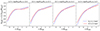 |
Fig. B.1. Fraction of the flux within different apertures over the flux in R500. The estimates are performed for two energy bands: 0.5 − 2.0 keV plotted with a red solid line and 0.2 − 2.3 keV with a dash-dotted blue line. The plots represent the medians obtained within the different halo mass bins. |
All Tables
Best-fit parameters for the completeness as a function of logarithmic input flux log S500.
All Figures
|
Fig. 1. X-ray scaling relations recovered from the halo population in the lightcone: with L500 − M500 in the left panel and L500 − kT500 in the right panel. The luminosity L500 is intended as the IGrM-only emission including Galactic absorption in the 0.1 − 2.4 keV band within R500. For reference, also literature values are reported: Lov+15 (Lovisari et al. 2015), Eck+11 (Eckmiller et al. 2011), Arn+10 (Arnaud et al. 2010). The masses and mass-weighted temperature are calculated in the same radius R500. Considering the small redshift range, we neglect any evolutionary changes in the scaling. |
| In the text | |
|
Fig. 2. Sky view of LC30 including all the X-ray sources modelled (i.e. IGrM, AGNs, XRBs, and background) with a zoom-in over one of the largest clusters and surrounding environment at the lowest snapshot. We report in red the extended detections and with yellow squares the point-source detections. The circles mark the extension of the source being R200 from the matched input catalogue. The orange rectangle at the top left shows the size of FOV for the eFEDS catalogue (i.e. 140 deg2). |
| In the text | |
|
Fig. 3. Distribution of the extended ℒEXT and detection likelihoods ℒDET for all the (candidate) extended sources. We colour-coded the points according to their angular scale in arcseconds. The red dashed lines mark the separation between the extent sources above the likelihood we choose to operate (i.e. ℒDET > 5 and ℒEXT > 6). |
| In the text | |
|
Fig. 4. Completeness profiles within the three different extent likelihood cuts (i.e. ℒEXT > 3, 6, 10). The completeness is defined in terms of the input flux S500 in the soft band (0.2 − 2.3 keV) in the top panel and the halo mass M500 in the bottom panel. We present the results for the sample with the extended (primary) detections with the solid lines. The dashed-dotted grey lines show the fraction of misclassified point sources: they are detections from the point source catalogue whose X-ray emission is at least 80% the IGrM in input. The coloured dotted lines are the best-fit curves. |
| In the text | |
|
Fig. 5. Comparison between the soft band luminosity recovered from the flux aperture in the mock observation and the input luminosity of the halos in the lightcone. The uncertainties are calculated as the 16th and 84th percentile from the MCMC run. We overplot the 1:1 relation in yellow and the best-fit relation in red. |
| In the text | |
|
Fig. 6. Soft band luminosity distribution of the groups and clusters in the lightcone in function of their redshift. The errors are the 16th and 84th percentile from the MCMC process to extract the luminosity. The data points are colour-coded for their extent likelihood. The shading areas represent the range of survey flux limits given by the completeness from 10% to 90% in steps of 10% difference with decreasing colour. The red curves represent the flux limit in eFEDS (1.5 × 10⁻¹⁴ erg s−1 cm−2; Liu et al. 2022c) and eRASS1 (10−13 erg s−1 cm−2; Seppi et al. 2022) for 40 and 30% completeness respectively. |
| In the text | |
|
Fig. 7. Comparison of the mass distribution in the input catalogue and derived from the scaling relation L500 − M500 in Lovisari et al. (2015). The errors are derived from the 16th and 84th percentile in the luminosity measurement. In dash-dotted yellow, we report the 1:1 relation; in dashed red the best fit from the scatter plot. Additionally, we determine the mass using the scaling relation derived from eFEDS data in Chiu et al. (2022) and plot its best fit as dotted blue. |
| In the text | |
|
Fig. 8. XLF of the intrinsic soft band (0.5 − 2.0 keV) for the extended sources in the lightcone. We plot the results for the full sample (solid blue line) and for only detected ones (dotted blue line). The shaded bands represent the Poisson uncertainty in the luminosity bin. Similarly, we show the XLF for the eFEDS (Liu et al. 2022c) and eRASS1 (Bulbul et al. 2024) data in orange and green respectively. For reference, we also add other results from the literature in black: the XXL-C1 sample (Adami et al. 2018) and the REFLEX II (Böhringer et al. 2014). |
| In the text | |
|
Fig. 9. XLF of the intrinsic soft band (0.5 − 2.0 keV) for the AGNs in the lightcone. The luminosities are not corrected for Galactic absorption. We report the results for both the detected population (dotted blue line) and the entire population (solid blue line). In orange, we plot the XLF extracted from the mock catalogue in Marchesi et al. (2020) properly rescaled to account for the survey volume difference. The shaded band illustrates the Poisson uncertainty. |
| In the text | |
|
Fig. 10. Median X-ray surface brightness of the extended detected (red) and undetected (blue) sources in the 0.5 − 2.0 keV for four different logarithmic halo mass bins (i.e. log(M200/M⊙) reported at the top of each panel). In the lower left of each panel, we report the number of detected and undetected in the mass bin. The shaded bands illustrate the 16th − 84th percentiles from the intrinsic distribution. |
| In the text | |
|
Fig. 11. Properties of the gas as a function of the scatter in the scaling relation L500 − M500 by Lovisari et al. (2015) in one halo mass bin (1013 − 1013.5 M⊙). From the top to bottom panels, we show temperature, metallicity, and gas fraction (all mass-weighted) measured within 0.15 R500 of each halo. The black line denotes the running median for each quantity. We also report the Spearman coefficient in the plot. |
| In the text | |
|
Fig. 12. Luminosity of the IGrM as a function of the fraction of hot gas within the same radius (i.e. R500). The halos are binned in logarithmic halo mass M200 (see legend). The shaded bands mark the 68th confidence intervals. |
| In the text | |
|
Fig. 13. Entropy of the hot IGrM measured within 0.15 R500. We plot it as a function of the scatter in the scaling relation L500 − M500 by Lovisari et al. (2015) in one halo mass bin (1013 − 1013.5 M⊙). |
| In the text | |
|
Fig. 14. Entropy within different radii as a function of the integrated temperature (within R500). The entropy is calculated for each halo as the ratio between the mass-weighted temperature and the electron density within that same radius. We calculate the running median for the detected (red), undetected (blue), and full sample (black). We plot the 25th − 75th percentiles with the shaded band. The black crosses represent the observational eRASS1 dataset from Bahar et al. (2024). The three images refer to three different radii (i.e. 0.15 R500, R2500, R500). We ensure halos host at least 80 gas particles within the selected aperture. |
| In the text | |
|
Fig. B.1. Fraction of the flux within different apertures over the flux in R500. The estimates are performed for two energy bands: 0.5 − 2.0 keV plotted with a red solid line and 0.2 − 2.3 keV with a dash-dotted blue line. The plots represent the medians obtained within the different halo mass bins. |
| In the text | |
Current usage metrics show cumulative count of Article Views (full-text article views including HTML views, PDF and ePub downloads, according to the available data) and Abstracts Views on Vision4Press platform.
Data correspond to usage on the plateform after 2015. The current usage metrics is available 48-96 hours after online publication and is updated daily on week days.
Initial download of the metrics may take a while.