| Issue |
A&A
Volume 699, July 2025
|
|
|---|---|---|
| Article Number | A127 | |
| Number of page(s) | 35 | |
| Section | Cosmology (including clusters of galaxies) | |
| DOI | https://doi.org/10.1051/0004-6361/202452466 | |
| Published online | 01 July 2025 | |
6 × 2 pt: Forecasting gains from joint weak lensing and galaxy clustering analyses with spectroscopic-photometric galaxy cross-correlations
1
Institute for Theoretical Physics, Utrecht University, Princetonplein 5, 3584CC Utrecht, The Netherlands
2
Leiden Observatory, Leiden University, Niels Bohrweg 2, NL-2333 CA Leiden, The Netherlands
3
Centro de Investigaciones Energéticas, Medioambientales y Tecnológicas (CIEMAT), Av. Complutense 40, E-28040 Madrid, Spain
4
Institute of Cosmology & Gravitation, Dennis Sciama Building, University of Portsmouth, Portsmouth PO1 3FX, UK
5
Waterloo Centre for Astrophysics, University of Waterloo, 200 University Ave W, Waterloo, ON N2L 3G1, Canada
6
Department of Physics and Astronomy, University of Waterloo, 200 University Ave W, Waterloo, ON N2L 3G1, Canada
7
Ruhr University Bochum, Faculty of Physics and Astronomy, Astronomical Institute (AIRUB), German Centre for Cosmological Lensing, 44780 Bochum, Germany
8
The Oskar Klein Centre, Department of Physics, Stockholm University, AlbaNova University Centre, SE-106 91 Stockholm, Sweden
9
Astrophysics Group and Imperial Centre for Inference and Cosmology (ICIC), Blackett Laboratory, Imperial College London, Prince Consort Road, London SW7 2AZ, UK
10
Donostia International Physics Center, Manuel Lardizabal Ibilbidea, 4, 20018 Donostia, Gipuzkoa, Spain
11
School of Mathematics, Statistics and Physics, Newcastle University, Herschel Building, NE1 7RU Newcastle-upon-Tyne, UK
12
Center for Theoretical Physics, Polish Academy of Sciences, al. Lotników 32/46, 02-668 Warsaw, Poland
13
Argelander-Institut für Astronomie, Auf dem Hügel 71, 53121 Bonn, Germany
14
Institute for Astronomy, University of Edinburgh, Blackford Hill, Edinburgh EH9 3HJ, UK
15
Department of Physics and Astronomy, University College London, Gower Street, London WC1E 6BT, UK
16
Aix-Marseille Université, CNRS, CNES, LAM, Marseille, France
17
Universität Innsbruck, Institut für Astro- und Teilchenphysik, Technikerstr. 25/8, 6020 Innsbruck, Austria
18
Shanghai Astronomical Observatory (SHAO), Nandan Road 80, Shanghai 200030, China
19
Key Laboratory of Radio Astronomy and Technology, Chinese Academy of Sciences, A20 Datun Road, Chaoyang District, Beijing 100101, P. R. China
20
University of Chinese Academy of Sciences, Beijing 100049, China
21
Institute for Particle Physics and Astrophysics, ETH Zürich, Wolfgang-Pauli-Strasse 27, 8093 Zürich, Switzerland
22
Department of Physics, Institute for Computational Cosmology, Durham University, South Road, Durham DH1 3LE, UK
23
Department of Physics, Centre for Extragalactic Astronomy, Durham University, South Road, Durham DH1 3LE, UK
⋆ Corresponding authors: This email address is being protected from spambots. You need JavaScript enabled to view it.
; This email address is being protected from spambots. You need JavaScript enabled to view it.
; This email address is being protected from spambots. You need JavaScript enabled to view it.
Received:
2
October
2024
Accepted:
23
April
2025
Abstract
Accurate knowledge of galaxy redshift distributions is crucial in the inference of cosmological parameters from large-scale structure data. We explore the potential for enhanced self-calibration of photometric galaxy redshift distributions, n(z), through the joint analysis of up to six two-point functions. Our 3 × 2 pt configuration comprises photometric shear, spectroscopic galaxy clustering, and spectroscopic-photometric galaxy-galaxy lensing (GGL). We expand this to include spectroscopic-photometric cross-clustering, photometric GGL, and photometric auto-clustering, using the photometric shear sample as an additional density tracer. We performed simulated likelihood forecasts of the cosmological and nuisance parameter constraints for stage-III- and stage-IV-like surveys. For the stage-III-like survey, we employed realistic redshift distributions with perturbations across the full shape of the n(z), and distinguished between ‘coherent’ shifting of the bulk distribution in one direction, versus more internal scattering and full-shape n(z) errors. For perfectly known n(z), a 6 × 2 pt analysis gains ∼40% in figure of merit (FoM) on the S8 ≡ σ8√Ωm/0.3 and Ωm plane relative to the 3 × 2 pt analysis. If untreated, coherent and incoherent redshift errors lead to inaccurate inferences of S8 and Ωm, respectively, and contaminate inferences of the amplitude of intrinsic galaxy alignments. Employing bin-wise scalar shifts, δzi, in the tomographic mean redshifts reduces cosmological parameter biases, with a 6 × 2 pt analysis constraining the δzi parameters with 2 − 4 times the precision of a photometric 3ph × 2 pt analysis. For the stage-IV-like survey, a 6 × 2 pt analysis doubles the FoM (σ8–Ωm) compared to the 3 × 2 pt or 3ph × 2 pt analyses, and is only 8% less constraining than if the n(z) were perfectly known. A Gaussian mixture model for the n(z) is able to reduce mean-redshift errors whilst preserving the n(z) shape, and thereby yields the most accurate and precise cosmological constraints for any given N × 2 pt configuration in the presence of n(z) biases.
Key words: cosmological parameters / cosmology: observations / dark energy / large-scale structure of Universe
© The Authors 2025
 Open Access article, published by EDP Sciences, under the terms of the Creative Commons Attribution License (https://creativecommons.org/licenses/by/4.0), which permits unrestricted use, distribution, and reproduction in any medium, provided the original work is properly cited.
This article is published in open access under the Subscribe to Open model. This email address is being protected from spambots. You need JavaScript enabled to view it. to support open access publication.
1. Introduction
Modern analyses of the large-scale structure (LSS) of the Universe frequently combine different cosmological probes to maximally leverage the available information, and break degeneracies between key parameters of the concordance model. One of the most powerful probes in use today is the weak gravitational lensing of light from distant galaxies (Bartelmann & Schneider 2001). The coherent ellipticity distortions induced by weak lensing modify galaxy isophotes at the percent level. We therefore require many millions of galaxy shapes in order to measure shear correlations at a sufficient signal-to-noise ratio (S/N) to constrain the underlying cosmology (Joudaki et al. 2017a; Hamana et al. 2020; Asgari et al. 2021; Secco et al. 2022; Amon et al. 2022; Longley et al. 2023). The next stage of experiments will expand on this endeavour by observing billions of galaxies.
Constraints derived from the lensing effect alone are subject to a strong degeneracy (Jain & Seljak 1997) between the amount of matter in the Universe today, Ωm, and its degree of clustering, parameterized by σ8 (the root mean square of the density contrast in spheres of radius 8 h−1 Mpc). Matter inhomogeneities source lensing convergence and shear fields that correlate with the cosmic density field. By sampling these fields at the positions of galaxies, one can probe density fluctuations in the aggregated dark and luminous matter distribution. The ‘3 × 2 pt’ method, which jointly analyses theauto- and cross-correlations of lensing and density fields, aids with the breaking of the σ8 − Ωm degeneracy, and has begun to yield cosmological parameter constraints that are competitive with the ones obtained via analyses of the cosmic microwave background (CMB) temperature and polarization anisotropies (Bernstein 2009; Joachimi & Bridle 2010; Krause & Eifler 2017; Joudaki et al. 2018; van Uitert et al. 2018; Abbott et al. 2018, 2022; Heymans et al. 2021). It has also been suggested that the cross-correlation of lensing and galaxy fields breaks the degeneracy between galaxy bias and the growth rate, which allows for stronger constraints on cosmic expansion scenarios (Bernstein & Cai 2011; Gaztañaga et al. 2012; Cai & Bernstein 2012). However, whether these gains are present for any other fundamental parameters or for calibrating lensing systematics has been unclear so far (Font-Ribera et al. 2014; de Putter et al. 2014). In principle, different tracers are sensitive to different redshift kernels, allowing for some of the degeneracies to be broken.
The increased precision of these constraints has revealed a mild tension between the late- and early-Universe determinations of the matter clustering parameter combination  , for which the CMB predicts a present-day value that is 2 − 3σ larger than the one observed by lensing experiments (Joudaki et al. 2017a,b, 2020; Hildebrandt et al. 2017; Leauthaud et al. 2017; Hikage et al. 2019; Hamana et al. 2020; Asgari et al. 2020; Tröster et al. 2021; Secco et al. 2022; Amon et al. 2022; Li et al. 2023; Dalal et al. 2023; More et al. 2023; Miyatake et al. 2023; Sugiyama et al. 2023). Resolving this tension, whether by better understanding experimental or theoretical limitations and assumptions (Longley et al. 2023; Dark Energy Survey and Kilo-Degree Survey Collaboration 2023), or with new physics (see Di Valentino et al. 2021; Joudaki et al. 2022; Abdalla et al. 2022, and references therein), is a primary goal of LSS cosmology. To this end, upcoming surveys are already making significant efforts towards implementing the 3 × 2 pt methodology within their analysis pipelines (Chisari et al. 2019a; Blanchard et al. 2020; Tutusaus et al. 2020; Sanchez et al. 2021; Prat et al. 2023).
In preparation for the next generation of experiments, the control of systematic errors in weak lensing analyses is more important than ever. The Euclid satellite (Euclid Collaboration: Mellier et al. 2025), the Vera C. Rubin Observatory (Ivezić et al. 2019), the Nancy Grace Roman Space Telescope (Spergel et al. 2015), the Canada-France Imaging Survey (CFIS-UNIONS; Ayçoberry et al. 2023), and the Chinese Space Station Telescope (CSST; Gong et al. 2019) will have to outperform their predecessors with regards to the effects and mitigation of photometric redshift uncertainty, intrinsic alignments of galaxies, baryonic feedback, shear mis-estimation, magnification bias, covariance mis-estimation, and various other sources of error. Of particular concern in recent years is the calibration of lensing source sample redshift distributions, n(z) (Mandelbaum et al. 2018; Joudaki et al. 2020; Schmidt et al. 2020; Euclid Collaboration: Desprez et al. 2020).
External calibration of photometric redshift distributions is an active field of research, and can be broadly categorized as using spectroscopic or high-quality photometric reference samples (e.g. Laigle et al. 2016; Padilla et al. 2019; Weaver et al. 2022; van den Busch et al. 2022) to either infer galaxy colour-redshift space relations (Hildebrandt et al. 2012, 2020, 2021; Leistedt et al. 2016a; Hoyle et al. 2018; Sánchez & Bernstein 2019; Hikage et al. 2019; Wright et al. 2020), or to measure positional cross-correlations (Newman 2008; Ménard et al. 2013; de Putter et al. 2014; Johnson et al. 2017; van den Busch et al. 2020; Gatti et al. 2022), or some combination thereof (Alarcon et al. 2020; Rau et al. 2021; Myles et al. 2021). Newman & Gruen (2022) review the recent literature on photometric redshifts and their challenges. While spectroscopy remains too expensive to provide an accurate redshift for every observed object, the modelling of lensing statistics only requires accurate knowledge of the redshift ‘distributions’ of source galaxy samples (Bernardeau et al. 1997; Huterer et al. 2006), rather than redshift point-estimates. Residual inaccuracies in the inferred redshift distributions are then typically modelled with nuisance parameters that are internally calibrated by the measured statistics, and marginalized over in the cosmological parameter inference.
The now-standard 3 × 2 pt formalism combines cosmic shear, galaxy-galaxy lensing (GGL), and galaxy clustering correlations, wherein positional samples are chosen to be the ones with spectroscopic redshift (or high-accuracy photo-z) information. Upcoming surveys are also considering leveraging the information in the clustering of photometric samples with low-quality photo-z (Nicola et al. 2020; Tutusaus et al. 2020; Sanchez et al. 2021). The prospective gains would be in area coverage, redshift baseline, and the number of objects, where the latter two increase greatly on approach to the survey magnitude limit. The concern lies in having control over spatially correlated, systematic density fluctuations induced by survey inhomogeneities (Leistedt et al. 2013, 2016b; Leistedt & Peiris 2014; Awan et al. 2016). However, new methodologies are now bringing this control within reach (Alonso et al. 2019; Rezaie et al. 2020; Johnston et al. 2021; Everett et al. 2022).
In either of those 3 × 2 pt strategies, redshift calibration remains a primary challenge. Collecting representative spectroscopic samples is currently infeasible at the depth of upcoming surveys (Newman et al. 2015). Clustering-based redshiftcalibration techniques are then expected to be prioritized over calibration with deep spectroscopic data (Baxter et al. 2022). However, this method can also suffer from some limitations coming from systematic errors in spectroscopic clustering measurements, sensitivity to an assumed cosmology, and clustering bias evolution, to name a few examples (Newman 2008). However, the photometric data themselves can also be used to avoid systematic biases or loss of precision. Schaan et al. (2020) demonstrated, for example, that photometric redshift scatter and outliers yield detectable clustering cross-correlations acrossredshift bins in photometric samples. These can improve the constraints on redshift nuisance parameters by an order of magnitude. This work takes a step further by exploring the possibility of enhancing internal redshift re-calibration through the inclusion of spectroscopic-photometric cross-correlations as additional probes within a joint analysis of two-point statistics. We propose extending the 3 × 2 pt formalism to include the cross-clustering of spectroscopic and photometric samples (4 × 2 pt), as well as the GGL and galaxy clustering measured within all-photometric samples, for a maximal 6 × 2 pt analysis.
Our analysis takes the form of a full simulated likelihood forecast for a current (stage III) weak lensing survey, and a complementary, simpler forecast for the upcoming generation of surveys (stage IV). We compute all unique cosmological and systematic contributor (intrinsic alignments, magnification) angular power spectra, C(ℓ), within and between two tomographic galaxy samples: a photometric sample tracing both the shear and density fields, with an uncertain redshift distribution to be modelled; and a spectroscopic sample tracing only the density field, and with a known redshift distribution.
We explore synthetic source distributions, n(z), with variations over the full shape of the function, choosing distributions for analysis that are ‘coherently’ shifted in terms of tomographic mean redshifts (all mean-redshift differences have the same sign), or ‘incoherently’ shifted (signs can be mixed), where calibration errors of the former kind are expected to manifest more strongly in S8 (Joudaki et al. 2020). We attempt to recover these shifted distributions through internal recalibration at and/or before the sampler stage, employing a selection of nuisance models for the task: scalar shifts, δzi, to be applied to the means of tomographic bins (e.g. Joudaki et al. 2017a; Asgari et al. 2021; Amon et al. 2022); flexible recalibration with the Gaussian mixture ‘comb’ model (Kuijken & Merrifield 1993; Stölzner et al. 2021), with and without additional scalar shifts; and a ‘do nothing’ model for characterizing the cosmological parameter biases incurred by different modes of redshiftdistribution calibration failure. A first observational demonstration of the viability of the comb marginalization procedure was provided in Stölzner et al. (2021), applied to stage III cosmic shear data. This work showed that an iterative calibration method of the comb amplitudes results in a good fit to the KV-450 cosmic shear data vector (the χ2 even improves by 1%). To achieve convergence both in the n(z) parametrization and cosmology, one starts from an already well-calibrated n(z) distribution and covariance.
Here, we report on the suitability of these redshift nuisance models for stage III and stage IV weak lensing analyses, and on the gains in accuracy and precision of cosmological inference to be derived from the inclusion of additional two-point correlations in the 6 × 2 pt analysis. In addition, we show how photometric redshift nuisance parameters can couple to other astrophysical systematics; namely, intrinsic galaxy alignments (Wright et al. 2020; Fortuna et al. 2021; Li et al. 2021; Secco et al. 2022; Fischbacher et al. 2023; Leonard et al. 2024).
This paper is structured as follows. Sect. 2 describes our modelling of the harmonic space two-point functions that form our analysis data-vector. Sect. 3 details our synthetic data products, and we present our forecasting methodology in Sect. 4. Sect. 5 displays and discusses the results of our forecasts, and we make concluding remarks in Sect. 6.
2. Theoretical modelling of two-point functions
The two-point functions considered as part of the data-vector in this work include all unique cross- and auto-angular power spectra between the positions of the spectroscopic sample and the positions and shapes of the photometric sample. For the spectroscopic sample, we restrict the analysis to angular power spectra (as opposed to the redshift-space multipole treatments of for example Gil-Marin et al. 2020; Bautista et al. 2021; Beutler & McDonald 2021) due to limitations in the analytical computation of the covariance between multipoles and angular power spectra, which we defer to future work (however, also see Taylor & Markovič 2022).
2.1. Angular power spectra in the general case
The angular power spectrum of the cross-correlation between galaxy positions (n) in two tomographic galaxy samples (α, β) is given by several contributions deriving from gravitational clustering (g) and lensing magnification (m),
 (2.1)
(2.1)
The indices, α, β, each run over the set of unique radial kernels employed in the analysis of Np photometric and Ns spectroscopic redshift samples.
Throughout this analysis, we made use of the Limber approximation (Limber 1953; Kaiser 1992; LoVerde & Afshordi 2008) in the computation of the angular power spectra. Although the Limber approximation is known to be insufficient for the level of accuracy required by future surveys, especially in the context of clustering cross-correlations across tomographic bins (Campagne et al. 2017), the computational cost of performing non-Limber computations of angular power spectra is currently prohibitive. In the near future, we expect our pipeline to be extended in this direction as new, fast, validated methods become suitable for embedding into full-likelihood analyses.
For now, we have limited our analysis to scales ℓ > 100 (Joachimi et al. 2021). We also neglected to include contributions derived from redshift space distortions (RSDs; Kaiser 1987), which should be small for these scales and principally affect the tomographic cross-correlations (Loureiro et al. 2019). Lastly, we restricted the clustering analysis to scales were the bias can be approximated as being linear (see Sect. 2.4 for details of other approximations made in this work).
Under the Limber approximation in Fourier space, the contribution attributed to pure gravitational clustering is
 (2.2)
(2.2)
where χH is the co-moving distance to the horizon,  and
and  are the linear biases of the galaxy samples, nα and nβ are the normalized redshift distributions of each sample, fK(χ) is the co-moving angular diameter distance, and Pδ is the matter power spectrum.
In addition, lensing magnification induces apparent excesses or deficits of galaxies above the flux limit of a survey due to the conservation of surface brightness of the lensed sources. Furthermore, the observed angular separation of galaxies behind the lenses are increased, diluting their number density. As a result, galaxy number counts pick up an additional contribution which is cross-correlated with the physical locations of galaxies that act as lenses. The result is three additional terms in the nn angular power spectra: the magnification count auto-correlation, ‘mm’,
 (2.3)
(2.3)
and the magnification count–number count cross-correlations, ‘mg’ and ‘gm’,
 (2.4)
(2.4)
where the gm term was constructed in exact analogy to the mg term by swapping the indices α and β. Magnification kernels,  , were derived from the respective lensing efficiency kernels, qα(χ), which are given by
 (2.5)
(2.5)
Multiplying  within the integrand of Eq. (2.5),
 (2.6)
(2.6)
yields the magnification kernel  . For tomographic sample, x, sx(χ) is the logarithmic slope of the magnitude distribution (e.g. Chisari et al. 2019a), and αx(χ) is that of the luminosity function (e.g. Joachimi & Bridle 2010) – not to be confused with the tomographic bin index, α. For computations of Fx, m(χ), we made use of the fitting formula for α given by Joachimi & Bridle (2010) (their Appendix C), assuming a distinct limiting r-band depth, rlim, for each of our synthetic samples (defined in Sect. 3).
The shape (γ) auto-spectrum is similarly given by several contributions,
 (2.7)
(2.7)
where ‘GG’ indicates a pure gravitational lensing contribution, given by
 (2.8)
(2.8)
The ‘I’ terms in Eq. (2.7) are well known to arise from intrinsic (local, tidally induced, as opposed to lensing-induced) alignments of the galaxies with the underlying matter field (Catelan et al. 2001; Hirata & Seljak 2004). These terms are known to cause biases in cosmological constraints if unaccounted for (Joachimi & Bridle 2010; Krause et al. 2016; Joudaki et al. 2017a). Moreover, they are expected to absorb residual biases in photometric sample redshift calibration if the nuisance model for alignments is too flexible and/or not specific enough (Wright et al. 2020; Fortuna et al. 2021; Li et al. 2021; Fischbacher et al. 2023).
The ‘GI’ contribution represents the lensing of background galaxy shapes by the same matter field that is responsible for the intrinsic alignments of foreground galaxies. This is given by
 (2.9)
(2.9)
and the case of ‘IG’ was analogously constructed by swapping the indices α and β. FIA(χ) represents an effective amplitude of the alignment of galaxies with respect to the tidal field as a function of co-moving distance. Although this formalism is strictly linear, it is common to use the nonlinear matter power spectrum in the computation of intrinsic alignment correlations (Bridle & King 2007).
The ‘II’ contribution in Eq. (2.7) is given by
 (2.10)
and represents the auto-correlation spectrum of galaxies aligned by the same underlying tidal field; it is thus expected to contribute more weakly to tomographic shear cross-correlations than the GI term, which can operate over wide separations in redshift.
The cross-correlation of lens positions and source shears forms the GGL component of the 3 × 2 pt analysis. This has several components:
 (2.11)
where the ‘gG’ term is the cross-correlation of galaxy positions and the shear field and is given by
 (2.12)
The ‘gI’ term in Eq. (2.11) arises through the cross-correlation of lens positions with source intrinsic alignments, and is expected to be non-zero only when the distributions nα, nβ are overlapping. This is given by
 (2.13)
The lensing magnification-induced number counts contribution in the foreground is also correlated with the background shears, creating the ‘mG’ term which is given by
 (2.14)
Finally, the magnification-induced number counts contribution yields an additional, weak cross-correlation with the intrinsic alignments’ contribution to the shapes, ‘mI’, given by
 (2.15)
2.2. Spectrum modelling choices
For our fiducial true Universe, we adopted the best-fit flat-Λ cold dark matter (ΛCDM) cosmology from Asgari et al. (2021) (their Table A.1, Col. 3; see also our Sect. 4 and Table 3), constrained by cosmic shear band-power observations from the public 1000 deg2 fourth Data Release of the Kilo Degree Survey (‘KiDS-1000’ Kuijken et al. 2019). Following Asgari et al. (2021), we modelled intrinsic alignments via the ‘non-linear linear alignment’ (NLA; Catelan et al. 2001; Hirata & Seljak 2004; Bridle & King 2007; Joachimi et al. 2011) model. This specifies the alignment kernel as
 (2.16)
where C1 is a fixed normalization constant (Bridle & King 2007) and D+(χ) is the linear growth function, normalized to 1 today (Joachimi et al. 2011). A1 was constrained to  by Asgari et al. (2021), though they (and Loureiro et al. 2022, who studied pseudo-Cℓ’s) saw that the best-fit alignment amplitude varied for different cosmic shear statistics.
In dealing with the biased photometric sample redshift distributions described in Sect. 3, we allowed for the distributions1, nα(z), to be recalibrated according to widely used (e.g. Joudaki et al. 2017a; Hikage et al. 2019; Asgari et al. 2021; Amon et al. 2022; Secco et al. 2022) bin-wise displacements of the mean redshifts, δzi. These displacements were applied for tomographic bin i as
 (2.17)
and were constrained by the two-point correlation data, and by Gaussian priors, the derivations of which are described in Sect. 3. We refer to this approach as the ‘shift model’, to be contrasted with a lack of nuisance modelling (the ‘do nothing’ model), and with the Gaussian mixture ‘comb’ models described below.
For the linear, deterministic galaxy biases, bgα, per-tomographic sample, α, we assumed a single functional form for the true bias, setting fiducial values for a magnitude-limited sample according to Mandelbaum et al. (2018):
 (2.18)
which was evaluated at the mean redshift, ⟨z⟩, for each sample redshift distribution, nα(z). This bias model was used up to an ℓmax compatible with  (see Sect. 4). Although we did not expect galaxy bias to remain linear up to this scale (Joachimi et al. 2021), we generated the data vector and analysed it with the same bias model, which still allowed us to draw comparisons across our different probe combinations and redshift error scenarios, and reduces computational expense. While the fiducial redshift-dependent bias model is the same for lenses and sources, in practice the bias parameters are varied per bin within a large prior range of [0.5, 9]. Pandey et al. (2025) investigated the impact of redshift evolution of the bias in the context of stage IV surveys and they showed that shifts induced in the cosmological parameters from ignoring this effect can be mitigated by including cross-correlations between redshift bins. As those are already included in our forecast, we would expect that even if modelled, the redshift evolution would be properly mitigated.
The matter power spectrum was emulated with CosmoPower (Spurio Mancini et al. 2022), relying on the Boltzmann code CAMB (Lewis et al. 2000; Howlett et al. 2012) and a correction for the effects of baryons following HMCode (Mead et al. 2015; Mead 2015). The amplitude of the matter power spectrum was effectively parametrized by As, the primordial power spectrum amplitude, although we sampled over ln(1010As) as it is more convenient for our implementation of CosmoPower (and is a more commonly used sampling variable; e.g. Planck Collaboration VI 2020 – for an assessment of the impact of this choice, see Joudaki et al. 2020). In contrast to Asgari et al. (2021), we assumed a cosmology with massless neutrinos. This was mainly chosen to reduce the computational cost, but we note that it would be valuable to explore the constraining power of (4−6) × 2 pt statistics on neutrino mass (e.g. Mishra-Sharma et al. 2018).
To account for the suppression of the matter power spectrum at small scales due to baryons (van Daalen et al. 2011; Chisari et al. 2019b), we used the HMCode20162 halo mass-concentration relation amplitude parameter, Abary, and followed Joudaki et al. (2018) in setting the halo bloating parameter, ηbary = 0.98 − 0.12Abary. For the true Universe, we assumed Abary = 2.8, differently to the best-fit Abary = 3.13 from Asgari et al. (2021) as the latter corresponds to a dark matter-only Universe, and we prefer to include some baryonic contributions in the fiducial data-vector. We note that Abary will in practice only be weakly constrained by stage-III-like forecasts, for which it is principally a parameter that will allow us to capture uncertainties in the modelling of the non-linear matter power spectrum. For stage-IV-like configurations, it is expected that baryonic feedback models should start to see meaningful constraints from weak lensing and combined probe analyses such as these – though a detailed investigation of hydrodynamic halo model constraints is beyond the scope of this work.
All of the observable two-point functions were calculated using the Core Cosmology Library (CCL)3 (Chisari et al. 2019a) in ‘calculator’ mode. As was previously mentioned, we did not include RSDs in our modelling due to constraints related to non-Limber computations. However, photometric surveys are known to be sensitive to RSDs (Ross et al. 2011; Tanidis & Camera 2019), which should therefore be included in follow-up work.
2.3. Angular power spectra for the Gaussian comb
The Gaussian ‘comb’ model decomposes the redshift distribution of a given tomographic bin of the photometric sample into a sum over NG Gaussian basis functions of fixed-width and uniformly spaced centres. Mathematically,
 (2.19)
for tomographic sample α, where amplitudes, Ai, must sum to unity for each sample, α, and each Gaussian basis function is given by (Stölzner et al. 2021)
 (2.20)
where zi and σcomb are the centre and width of basis function ni(z), and the normalization over the interval z ∈ [0, ∞] is given by
 (2.21)
where σ ≡ σcomb. The concatenated vector of α tomographic redshift distributions is then ncomb(z), which we can fit to an arbitrary redshift distribution, N(z), with associated covariance, Σn(z) (see Sect. 3.1.1), by varying amplitudes, amμ = lnAmμ, to minimize the χn(z)2 given by
 (2.22)
where k, l index the elements of the concatenated redshift distribution vectors and the covariance, Σn(z). We refer to this model distribution as the ‘initial comb’ model, ncomb, ini(z), which can be used directly in theoretical computations of angular power spectra (e.g. Eq. (2.2)).
Taylor & Kitching (2010) and Stölzner et al. (2021) detailed the construction of analytical expressions for the two-point function likelihood, with marginalization over some nuisance parameters (the comb amplitudes) given a prior. They also derived expressions for the displacement in the sub-space of nuisance parameters from the peak of the likelihood, dependent upon derivatives of the log-likelihood with respect to those parameters. Minimizing that displacement by iteratively varying the amplitudes (and cosmological or other parameters, when the fiducial set is unknown); recomputing angular power spectra; and evaluating the likelihood derivatives, one obtains the ‘optimized comb’ model ncomb, opt(z).
During the initial fitting (Eq. (2.22)), comb amplitudes, Amμ, are often seen to be consistent with zero, leading to concerns about the suitability of Gaussian priors for the parameters, amμ. Taylor & Kitching (2010) also give expressions for flat priors, but these too are difficult to motivate; the choice of a lower boundary in the range [ − ∞, 0] is somewhat arbitrary for a 1-d likelihood that asymptotes to a constant as amμ → − ∞, and yet it is highly consequential for the marginalization. We therefore defer a full 6 × 2 pt application of the comb model (with optimization and marginalization as demonstrated by Stölzner et al. 2021) to future work, for which an extension to describe spectroscopic-photometric cross-correlations is currently under development.
Meanwhile, we obtained the optimized comb model, ncomb, opt(z), in this work by varying comb amplitudes, amμ, to minimize the fiducial two-point, χd2, given by
 (2.23)
for data- and theory-vectors, d and μ, respectively, and data-vector covariance Z (Sect. 2.5), each indexed by i, j. The comb optimization procedure is thus:
-
Begin with some data-vector, d, sourced from an unknown redshift distribution, n(z);
-
Fit an initial comb model, ncomb, ini(z), directly to a possibly biased ‘estimate’ of the distribution, N(z), with its associated covariance, Σn(z);
-
Estimate the theory-vector, μ, using ncomb, ini(z);
-
Minimize Eq. (2.23) by adjusting the comb amplitudes, amμ, resulting in an optimized comb model, ncomb, opt(z), which has been flexibly recalibrated against information from the data-vector.
The amplitudes, amμ, of the optimized comb model, ncomb, opt(z), were then fixed during the sampling of cosmological and nuisance model parameters. This iterative procedure allows us to reduce the computational expense of varying comb amplitudes at the same time one samples the likelihood.
We henceforth refer to this method as the ‘comb model’, denoted as 𝒩comb. In practice, however, we still seek to marginalize over some uncertainty in the redshift distribution, and do so through combination with the commonly used shift model (δzi; described in Sect. 2.1), whereby scalar shifts are applied via Eq. (2.17) to the optimized comb model ncomb, opt(z) during likelihood sampling, and later marginalized over. We refer to this hybrid as the ‘comb + shift’ model, denoted as 𝒩comb + δzi. As we shall see in Sect. 4, the comb models reveal the insufficiency of the shift model for application to photometric density statistics, whilst also offering generally superior recoveries of the true lensing efficiency kernel q(χ).
2.4. Approximations
Over the course of this work, we found that extended-analysis inference simulations were particularly slow to converge, with 6 × 2 pt chains potentially taking multiple weeks to reach convergence, even when using fast nested sampling algorithms such as MultiNest (Feroz & Hobson 2008; Feroz et al. 2009, 2019). This is primarily due to rapidly decreasing acceptance fractions that become extremely small, 𝒪(10−2), on the approach to convergence (to be discussed in Sect. 5.5), and the large number of Limber integrations required to fully characterize the enlarged theory-vectors.
This computational demand led us to the approximations already discussed: one-parameter linear galaxy bias and alignments; emulated matter power spectra with a one-parameter baryonic feedback model; Limber-approximate angular power spectra without RSDs; and massless neutrinos. Many of these choices are insufficient to describe the real Universe with the accuracy required by future surveys, but together they greatly increase the speed of the likelihood evaluation. Given that we applied scale cuts to density probes, which lessen the impact of these choices (Sect. 4; Eq. (4.1)), and given our intention to investigate the potential gains from 6 × 2 pt ‘relative’ to (1−3) × 2 pt analyses, we made some further approximations in our application of kernel modifiers for intrinsic alignment and magnification contributions to enhance the computational speed.
To reduce the required number of integrations over χ, we made the following transformations:
 (2.24)
where  was evaluated at the mean of the kernel product n(χ)q(χ), or n(χ)n(χ), and
  took the luminosity function slope, αx(⟨z⟩), at the mean redshift of sample x (see Appendix A in Joachimi & Bridle 2010, where the slope is evaluated at the sample median redshift). Provided that the Limber integration kernels (Sect. 2.1) have relatively compact support – as is the case for narrow spectroscopic bins (Sect. 3), but less so for broad photometric bins – these approximations will not yield unrealistic spectra, at least in the context of linear models for IA and magnification.
An illustration of these, and the linear galaxy bias approximations, is given in Fig. 1, where our mock stage III photometric and spectroscopic redshift distributions (to be described in Sect. 3) are reproduced in each panel and overlaid with the functional forms for  and FIA(z). Circular points atop each curve mark the mean redshifts of photometric (black) or spectroscopic (colours) redshift samples, at which the galaxy bias and magnification kernels are evaluated (FIA(z) is evaluated at the means of kernel products).
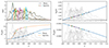 |
Fig. 1. Top left: Photometric (black curves and thin faint curves, corresponding to different realizations of the redshift distribution; described in Sect. 3.1.1) and spectroscopic (coloured curves) tomographic redshift distributions utilized in this work (described in Sect. 3) for a stage III survey. Top right: Galaxy bias function (blue curve; Eq. (2.18)) used to define the true galaxy bias, bg, for each tomographic redshift sample. Bottom left: Magnification bias functions, Fm(z) (Eq. (2.6)), used to calculate lensing contributions to galaxy number count kernels (Sect. 2.1), shown on a log-linear axis with transitions at ±1. The faint-end slope of the luminosity function is estimated via the fitting formulae of Joachimi & Bridle (2010), taking the r-band limiting magnitude rlim = 24.5 for the photometric (blue curve) and rlim = 20.0 for the spectroscopic (dashed orange curve) synthetic galaxy samples. Bottom right: Intrinsic alignment power spectrum prefactor function FIA(z) (blue curve; Eq. (2.16)) used to approximate matter-intrinsic and intrinsic-intrinsic power spectra for the computation of intrinsic alignment contributions to the shear and GGL correlations. The galaxy bias bg(z) and magnification bias Fm(z) functions are evaluated for each tomographic sample i at the mean redshift ⟨z⟩i of the sample, denoted by black (photometric) or coloured (spectroscopic) points atop each curve. The intrinsic alignment prefactor FIA(z) also displays these points but is evaluated at the mean of the relevant kernel product ni(χ)nj(χ), or ni(χ)qj(χ), for a correlation between samples i and j. |
We find that the  approximation results in cosmic shear spectrum (Eq. (2.7)) deficits of ≲0.03σ, for the uncertainty, σ, on each respective shear signal (see Sect. 2.5 for details on signal covariance estimation). Interestingly, the
  approximation is comparatively more consequential; through scale-dependent modifications to mg/gm (mm is largely unaffected) contributions (Eq. (2.4)), the total clustering signals (Eq. (2.2)) are suppressed by 0.05σ − 0.8σ, dependent upon the tomographic bin pairing, and most severely at high-ℓ. Our application of scale-cuts thus reduces the proportion of strongly suppressed points entering the data-vector – only a slim minority of our analysed clustering C(ℓ)’s are suppressed by more than 0.3σ, and the majority of clustering S/N comes from relatively unbiased points. We note that number counts from lensing magnification are commonly modelled according to such averages over αx(χ) (Garcia-Fernandez et al. 2018; von Wietersheim-Kramsta et al. 2021; Mahony et al. 2022a; Liu et al. 2021). It is likely that future analyses will need to explicitly integrate over the magnification kernel in order to accurately model these contributions (see also the recent work of Elvin-Poole et al. 2023, for a more rigorous treatment of magnification bias in samples with complex selection functions). We emphasize that the inaccuracies induced by our approximations apply to all forecasts under consideration, such that we make like-with-like comparisons when analysing the results for different two-point probe combinations.
With linear factors extracted from the Limber integrals, we are able to reduce the number of required Limber integrations by about an order of magnitude by reusing the ‘raw’ angular power spectra for each unique kernel product, nα(χ)nβ(χ),nα(χ)qβ(χ), or qα(χ)qβ(χ). Each is then re-scaled by relevant factors of bg,  , and/or
  correspondingly to produce appropriate spectral contributions for each probe. Thus, we give up some small amount of realism from explicit integrations over various kernels describing the different density, magnification, shear, and alignment contributions, in exchange for large gains in computational speed through the reuse of factorisable Limber integrations. Sampling in parallel with 40–48 cores, the resulting stage III chains take hours (sometimes less than one) to converge for (1−3) × 2 pt, and up to a few days for 6 × 2 pt, which is tractable for our purposes here.
We recommend that future work make use of emulators for Boltzmann computations, and explore the possibility of extending the emulation to the level of Cℓ’s or other observables. We particularly recommend this in the context of extended models with additional parameters, for example, for IA (Blazek et al. 2019; Vlah et al. 2020) and galaxy bias (Modi et al. 2020; Barreira et al. 2021; Mahony et al. 2022b), and of such theoretical developments as non-Limber integration for the utilization of large-angle correlations (e.g. Campagne et al. 2017; Fang et al. 2020), each of which is likely to prove especially costly for joint analyses of multiple probes (Leonard et al. 2023).
2.5. Analytic covariance estimation
We assume a Gaussian covariance throughout this analysis, since Gaussian contributions should dominate the error budget for the scales that we consider (Sect. 4; Eq. (4.1)). We homogenize the analysis choices and approximations across our forecast (Sect. 2.4) and make like-with-like comparisons when quoting results. Whilst future work should consider connected non-Gaussian and super-sample covariance contributions to the signal covariance, especially in the 3–6 × 2 pt case (Barreira et al. 2018a,b), we assume that these would not significantly affect our conclusions, which come from comparing across different probe combinations while always adopting a Gaussian covariance.
The Gaussian covariance matrix, Z ≡ Cov[d, d′], is entirely specified by the power spectra. Given Wick’s theorem, one finds
![Mathematical equation: $$ \begin{aligned} \mathrm{Cov} [C^{ij}(\ell ), C^{mn}(\ell \prime )] = \frac{\delta ^\mathrm{K} _{\ell \ell \prime }}{f_\mathrm{sky} N_\ell }\left(\hat{C}^{im}(\ell )\hat{C}^{jn} (\ell \prime ) + \hat{C}^{in}(\ell )\hat{C}^{jm} (\ell \prime )\right), \end{aligned} $$](/articles/aa/full_html/2025/07/aa52466-24/aa52466-24-eq41.gif) (2.25)
(2.25)
where fsky is the sky fraction of the survey, 4πfsky = Asurvey, i, j, m, n label any tracer in the analysis, and  is the observed angular power spectrum, which includes noise. In other words,
 (2.26)
where  is the Dirac delta function, σϵ2 is the single-component ellipticity dispersion, and
  is the average number density of sources (shear sample objects) or lenses (position sample objects) for each tracer (see Joachimi et al. 2021 for more details). The factor, Nℓ, in Eq. (2.25) counts the number of independent modes at multipole ℓ,
 (2.27)
where Δℓ is the bandwidth of each multipole bin used in the analysis. It should be noted that the covariance was calculated from the same n(z) as the mock-data (see Sect. 3 for the sampling of the mock-data); therefore, it was derived from the true n(z) and did not change during the sampling. Furthermore, if two statistics were measured over a different sky area we take the maximum between the two areas in the sky fraction and similarly for overlapping surveys (e.g. van Uitert et al. 2018).
3. Synthetic data products
We define here several synthetic galaxy samples with which to conduct our angular power spectrum analysis forecasts, summarizing their characteristics in Table 1.
Synthetic stage III and stage IV galaxy samples.
3.1. Mock stage III samples
For our stage III forecasts, we based our synthetic samples on those used for the cosmic shear and combined-probe analyses of KiDS-1000 (Asgari et al. 2021; Giblin et al. 2021; Hildebrandt et al. 2021; Heymans et al. 2021; Joachimi et al. 2021; Tröster et al. 2021). The strategy for generating the data-vector and covariance for our stage III forecast is summarized in Fig. 2.
 |
Fig. 2. Sketch of how the data-vector and covariance are generated for our stage III forecasts. |
3.1.1. KiDS-1000-like photometric sample
With the exception of the redshift distributions, we defined our stage III photometric samples to directly resemble those of the public KiDS-1000 data. We substituted the redshift distributions of KiDS-1000 calibrated via self-organizing maps (SOMs; Hildebrandt et al. 2021; Wright et al. 2020) for the earlier KiDS+VIKING-450 (KV450) direct redshift calibration of Hildebrandt et al. (2020) and Wright et al. (2019), from which a full covariance of the n(z) could be reliably derived owing to the spatial bootstrapping approach utilized. We used this covariance to generate additional redshift distributions which are biased with respect to the starting distribution, as we shall describe below.
Whilst the KV450 and KiDS-1000 redshift distributions are similar, we did not require the distributions to correspond closely to the latest KiDS n(z) calibration because we are conducting a simulated analysis, and we are free to choose the true and biased n(z) accordingly. We did assume that the n(z) covariance is reasonably realistic, and note that any future forecasting analysis conducted along these lines would do well to utilize a covariance derived from the latest calibration, incorporating state-of-the-art methods as far as possible.
To define (un)biased redshift distributions, we applied the following procedure. We began by assuming the KV450 redshift distribution, N(z), evaluated at 41 equally spaced redshifts z ∈ [0, 2], to represent the mean of a multivariate Gaussian distribution, that is, the calibrated covariance, Σn(z). The correlation matrix corresponding to Σn(z) is shown in Fig. 3, where labels ni(z) in the figure denote the tomographic bins i ∈ {1, 2, 3, 4, 5}. We then drew ∼45 000 realizations of the full n(z) (> 200 times the number of calibrated data points in a single n(z), across all five bins) from the multivariate normal distribution 𝒩(0, Σn(z)) and added these to the mean distribution, given by N(z)4, to yield an ensemble of redshift distributions {n(z)}X. Approximately 80% of the realizations in the ensemble had one or more negative n(z) values and were consequently discarded, such that X refers to the ones remaining.
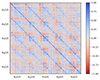 |
Fig. 3. Matrix of correlation coefficients corresponding to the covariance, Σn(z), of the five-bin tomographic redshift distribution (see also Figs. 1 and 4) estimated for the KiDS+VIKING-450 data release (Hildebrandt et al. 2020; Wright et al. 2019) via direct redshift calibration. The covariance is estimated through spatial bootstrapping of spectroscopic calibration samples (see Hildebrandt et al. 2020 for more details), and axis labels illustrate the subsections of the matrix corresponding to each of the five tomographic bins ni(z). The covariance is used to describe a multivariate Gaussian sampling distribution for realizations of photometric redshift distributions (Sect. 3.1.1). |
For each of the remaining realizations, we then computed the 5-vector of mean redshifts, ⟨z⟩i, of each tomographic bin and defined the quantities
 (3.1)
(3.1)
where ⟨z⟩i0 denote the mean redshifts of the starting distribution N(z). Thus, Δincoherent describes the Euclidean distance of a sampled n(z) from the mean of the multivariate normal distribution, N(z), after compressing to the five mean redshifts, and can be large regardless of the signs of the deviations, ⟨z⟩i − ⟨z⟩i0 (≡δzi; Sect. 2.2). Conversely, Δcoherent describes a post-compression distance from N(z) that is large only if the deviations are of the same sign; that is, if the total n(z) realization is coherently shifted to higher or lower redshifts across all five bins.
Sorting the ensemble {n(z)}X according to these Δ quantities, we then selected three realizations of redshift distributions:
-
the unbiased, or in practice least biased, redshift distribution
 , to minimize Δincoherent;
 -
the incoherently biased redshift distribution
 , to maximize Δincoherent;
 -
the coherently biased redshift distribution
 , to maximize Δcoherent.
As a consequence of the fixed covariance, Σn(z), the sorting order of {n(z)}X by (in)coherent bias in tomographic mean redshifts is similar. We therefore chose  first and imposed that
  , and that the deviations in mean redshifts ⟨z⟩i − ⟨z⟩0 should not all have the same sign for
  . Under these conditions, the Δincoherent and Δincoherent statistics for
  are ∼27% and ∼74% larger, respectively, than the ones seen for
  . However, defining a third distance quantity as a simple Euclidean distance over the full n(z) shape,
 (3.2)
(3.2)
where i still indexes tomographic bins and j indexes the redshift axis, we see that Δfull is ∼33% larger for our chosen  than for
  . Despite being less deviant in the mean redshifts, the incoherently biased distribution is in totality more deviant from N(z) than is
  . Since we are interested in the differential impacts upon cosmological constraints of (i) coherent shifting of the bulk redshift distribution, and (ii) more stochastic errors within the distribution, these choices suit our purposes and we proceeded accordingly. We note that a more detailed follow-up analysis could explore several such choices for (in)coherently biased distributions, perhaps using the full shape distance as another metric for the selection, and making use of different Σn(z) that yield more heterogeneous ensembles {n(z)}X.
The resulting distributions are shown in Fig. 4, where the mean distribution N(z) is given by black curves; the unbiased distribution by green curves; the incoherent bias by dash-dotted orange curves; and the coherent bias by dashed purple curves. Alternating panels show the distributions, n(z), and the differences, Δn(z) = n(z)−N(z), for each of the chosen redshift bias scenarios. The n(z) are also shown in faint grey for a random 50 realizations from the initial 45 000 ensemble. Inset panels display the high-z tail for each bin on a logarithmic y axis and reveal excesses relative to the starting N(z), particularly in the case of the coherent bias (purple).
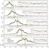 |
Fig. 4. Five-bin stage III photometric redshift distributions employed in our forecasts, with alternating panels showing the distribution ni(z) of bin i and its difference Δni(z) = ni(z)−Ni(z) with respect to the ‘mean’ distribution Ni(z). Black curves in each panel correspond to the mean distribution N(z), taken as the final, public KiDS+VIKING-450 estimate (Hildebrandt et al. 2020; Wright et al. 2019). As described in Sect. 3.1.1, we assume a multivariate Gaussian distribution described by the mean N(z) and covariance Σn(z) (Fig. 3) to generate 45 000 sample redshift distributions, a random 50 of which are shown in n(z) panels as faint grey curves. After discarding the 80% of samples with negative n(z) values, the tomographic mean distance metrics Δincoherent and Δcoherent (Eq. (3.1)) are used to select the most deviant (with respect to the mean N(z)) of the remaining samples: the ‘incoherently’ |


It is expected that a coherent bias in the redshift distribution used to model cosmic shear statistics should manifest more strongly in the final inference of the structure growth parameter, S8, than an incoherent redshift bias (see e.g. Joudaki et al. 2020, and the recent work of Giannini et al. 2024). This is because the same measured weak lensing signal, assumed to originate from a higher redshift, would be consistent with a lower S8 value if all else is held constant. We note too that all distributions, including  , feature full-shape differences with respect to the mean distribution N(z) (e.g. second Δn(z) panel in Fig. 4); such localized features are more likely to manifest in the density statistics, particularly the photometric auto-clustering.
Our central proposal is that nuisance models designed to compensate for any such errors in redshift calibration will enjoy more accurate and precise constraints upon the inclusion of additional two-point correlations in a joint analysis (similarly to the proposal of Joachimi & Bridle 2010, in the context of intrinsic alignment calibration), particularly the spectroscopic-photometric clustering cross-correlations. It is therefore important that the photometric shear and density samples share a redshift distribution (Schaan et al. 2020). This implies that any weighting of the shear sample (e.g. as derived from shape measurements) that is incorporated into the redshift calibration must also be applied to the photometric density sample5.
For each of our forecasts, the true n(z) distribution that enters the computation of our mock data-vector is given by one of the above-defined distributions: unbiased, incoherently biased, or coherently biased (or the exact N(z), for limited use), as described in Sect. 2. Meanwhile, the N(z) that enters the theory-vector computation is an externally calibrated estimate for the photometric sample redshift distribution, which we refer to as the exact N(z), with or without the application of nuisance models (Sect. 2.2)6. We henceforth refer to the redshift bias configurations as: ‘incoherent’, where the tomographic mean redshifts are systematically low at low redshift (i.e. pertaining to the starting distribution relative to the target distribution informing the data-vector), but more accurate as the redshift increases; ‘coherent’, where the mean redshifts are systematically low at all redshifts; and ‘unbiased’, where the mean redshifts are accurate (see Fig. 4). All three configurations feature full-shape errors in the redshift distribution. We also make limited use of the N(z) distribution, without additional modelling, as the source of both data- and theory-vector, referring to this as the ‘exact-true’configuration.
We emphasize here that our different n(z) bias cases yield different data-vectors; the (in)coherently biased cases are sourced from generally higher redshifts than the unbiased/exact-true cases (Table 1). Consequently, the addition of nuisance model parameters can counter-intuitively increase the overall constraining power, if the parameters act via the n(z) to push signals into regimes of higher S/N (aided in our case by the application of nonzero-mean Gaussian priors for δzi parameters; to be discussed more in Sect. 5). Although this also complicates direct comparisons with previous work on real data (e.g. Joudaki et al. 2020), where the theory-vectors are variable through n(z) estimates and nuisance modelling but the galaxy data are fixed, the qualitative results are in agreement.
We note that our methods of defining biased redshift distributions constitute a mixture of pessimistic and optimistic choices. Whilst we drew many thousands of realizations, and chose serious outliers to describe the true distributions, these are all compatible with the calibrated covariance; thus, they do not represent catastrophic failures of redshift calibration, but uncommon realizations. When sampling, we assumed uncorrelated Gaussian priors (Sect. 4; Table 3) for use with the shift model (Sect. 2.2) that are centred on the true shifts, δzi = ⟨z⟩i − ⟨z⟩i0, and have widths corresponding to the true variance of δzi over the ensemble {n(z)}X; thus, the calibration is assumed to yield a perfectly accurate prior for δzi in each case. Lastly, we have selected these n(z) only considering variations in the tomographic mean redshifts, δzi. It may be that an equivalent consideration of the full n(z) shape, for example, via metrics like Δfull, would yield distributions of different profiles, carrying distinct consequences for cosmological parameter inference under probe configurations variably sensitive to the full shape of the n(z) and the tomographic mean redshifts. Each of these choices could be revisited in future analyses of the impacts of redshift distribution mis-estimation.
The shear dispersion and effective number density statistics of the photometric sample are taken to be exactly those estimated for the KiDS-1000 shear sample, given in Table 1 of Asgari et al. (2021). Bin-wise mean redshifts, ⟨z⟩, were computed for  and
and  , while the means of
  are practically the same as for N(z). These are given in Table 1, which also records the assumed r-band depth, rlim = 24.5, and area = 777 deg2 for our stage III photometric survey set-up.
3.1.2. BOSS-2dFLenS-like spectroscopic sample
For synthetic spectroscopic samples, we took the combined redshift distribution of SDSS-III BOSS (Eisenstein et al. 2011) and 2dFLenS (Blake et al. 2016), presented for KiDS-1000 usage by Joachimi et al. (2021). As was mentioned in Sect. 2, an analytical consideration of the covariance between angular power spectra and three-dimensional multipole power spectra is under development. In the meantime, we attempted to retain the three-dimensional density information from the mock spectroscopic sample by finely re-binning the spectroscopic n(z), defining 10 tomographic samples in the range z ∼ 0.2 − 0.75, each having width Δz ∼ 0.05 (see Loureiro et al. 2019 for a similar treatment of BOSS DR12). We recomputed the mean redshifts ⟨z⟩i, re-scale the number density statistics from Joachimi et al. (2021) for each newly defined redshift bin, and record these figures in Table 1 along with the assumed area of 9329 deg2. For spectroscopic-photometric cross-correlations, we assumed an overlapping area of 661 deg2 (the sum of BOSS+2dFLenS versus KiDS-1000 overlapping areas; Joachimi et al. 2021) and retained the number densities and bin-wise redshift distributions of the full spectroscopic sample.
We assumed an r-band depth of rlim = 20.0 for the stage III spectroscopic samples in order to roughly match the luminosity function slopes, αx(z), observed by von Wietersheim-Kramsta et al. (2021) for BOSS data. The αx(z, rlim) that result from this magnitude limit via the fitting formulae of Joachimi & Bridle (2010) are slightly low for the lower-z spectroscopic bins, and high for the higher-z bins, and do not allow for significantly improved agreement through changes to rlim. This is likely due to the complex selection function defining BOSS galaxy samples, resulting in luminosity functions that are not well described by the fitting formula of Joachimi & Bridle (2010), which is calibrated against magnitude-limited galaxy data. A more principled estimation of αx(z), perhaps using luminosity functions directly, or using simulations (Elvin-Poole et al. 2023), would be desirable for more accurate modelling of magnification number count contributions in future work.
3.2. Mock stage IV samples
We defined mock stage IV samples based on information from the Science Requirements Document (SRD) of the Rubin Observatory Legacy Survey of Space and Time (LSST) Dark Energy Science Collaboration (DESC; Mandelbaum et al. 2018). These are supplemented by mock spectroscopic samples, modelled after the survey specifications of the Dark Energy Spectroscopic Instrument (DESI; DESI Collaboration 2016). The strategy for generating the data-vector and covariance for our stage IV forecast is summarized in Fig. 5.
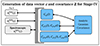 |
Fig. 5. Sketch of how the data-vector and covariance are generated for our stage IV forecasts. |
3.2.1. LSST Y1-like photometric sample
For our stage-IV-like photometric dataset, we assumed the LSST Year 1 redshift distribution from the SRD, given by
 (3.3)
(3.3)
which we evaluated over the range z = 0 − 4. Also following the SRD, we defined the shear sample to have five equi-populated bins over this range and convolved each of these with a Gaussian kernel of evolving width σz = 0.05(1 + z) in order to simulate photometric redshift errors.
We went beyond the SRD for our forecasts, additionally defining a biased redshift distribution. To do so, we simply drew random shifts, δzi, from the normal distributions, 𝒩(0, σshift), where σshift = [0.01, 0.02, 0.03, 0.04, 0.05] for the five bins, respectively, and applied these to the starting distributions ni(z) as  . Without any restriction on the sign of the shifts, these more closely resemble the incoherently biased stage III redshift distributions from Sect. 3.1.1. We assessed the ability of the shift model to correct these redshift errors (given Gaussian priors centred on the true δzi, with widths equal to σshift), noting that redshift biases constructed in this way are unrealistic and overly generous to the shift model; future forecasts should consider more complex, full-shape n(z) biases, as we have done in our stage III set-up (Sect. 3.1.1). We accordingly differentiate between the full-shape, (in)coherently biased stage III redshift distributions, and the ‘shifted’ distributions considered for stage IV.
By construction, each of the tomographic bins has a similar number density, which we computed after assuming the full sample to have 10 galaxies arcmin−2 and re-binning the total n(z). We followed the SRD in assuming an intrinsic shear dispersion of σϵ = 0.26, an r-band depth of rlim = 25.8, and an area of 12 300 deg2 for LSST Year 1 – these statistics, and per-bin mean redshifts ⟨z⟩i, are recorded in Table 1.
We note that photometric data are already intended for usage as density samples in the analysis of LSST (Mandelbaum et al. 2018). However, these lens samples are to be defined with uniform spacing in redshift, and with limits such that z ∈ [0.2, 1.2]. Our forecasts here presume that the shear sample itself can be used for density statistics (similarly to Joudaki & Kaplinghat 2012; Schaan et al. 2020), with redshift distribution recalibration bolstered by cross-correlations with a spectroscopic density sample, given the overlap between LSST and DESI.
3.2.2. DESI-like spectroscopic samples
We considered 4000 deg2 of DESI-like spectroscopic observations, which completely overlap with our LSST Year 1-like samples (Mandelbaum et al. 2018). For simplicity, we assumed this as a conservative area coverage for the DESI Year 1 data, noting that the true coverage is nearly twice as large. We took the forecasted redshift distributions dN/dzdΩ (where Ω denotes a solid angle) for the DESI bright galaxy sample (BGS), emission line galaxy (ELG) sample, and luminous red galaxy (LRG) sample7 from DESI Collaboration (2016), Tables 2.4 and 2.68, and re-binned them to have uniform widths of at least Δz = 0.2, resulting in 11 tomographic bins (BGS:2, ELG:6, LRG:3) that share some internal overlaps in the range z ∼ 0.5 − 1.0. We note that these spectroscopic bins are ∼4× wider (in redshift space) than those implemented in our stage III set-up; this choice was made only to reduce the computational demand of these forecasts, and finer tomography is a primary avenue for improvement in future work. Indeed, the calibration power of cross-correlations estimated here for stage IV analyses could be considered as conservative, though this is offset by the simplicity of the implemented redshift errors (Sect. 3.2.1).
Given the area coverage and newly defined redshift distributions, number densities per bin have simply been calculated and recorded in Table 1 alongside mean redshifts, ⟨z⟩i. Targeting surveys for DESI were estimated to yield an r-band depth of at least rlim = 23.4, which we assumed to be the limiting magnitude for each of the mock DESI galaxy samples for simplicity. The αx(z) so-estimated from the fitting formula (Joachimi & Bridle 2010) are again unlikely to describe well the luminosity functions of these highly selected DESI samples. We are therefore modelling magnification contributions for these (and to a slightly lesser extent the stage III) samples according to rough guesses of reasonable values for the slopes of luminosity functions – since these are minor contributions to clustering correlations, and since we neither vary nuisance parameters to describe magnification contributions (see for example Elvin-Poole et al. 2023), nor fail to model them entirely (see Mahony et al. 2022a, for the impact of faulty modelling), we do not expect these choices to affect our conclusions. Our stage IV sample redshift distributions are depicted in Fig. 6, with LSST year-1-like photometric samples in the top panel, and DESI-like spectroscopic samples in the bottom panel (including the prospective, sparse, high-z quasar – ‘QSO’ and ‘Lyman-α QSO’ – samples that we do not consider in this work due to computational constraints).
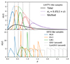 |
Fig. 6. Redshift distributions assumed for our stage IV synthetic galaxy samples, with LSST year-1-like photometric tomography (top; Sect. 3.2.1), supplemented by DESI-like spectroscopic galaxy samples (bottom; Sect. 3.2.2). Vertical dotted lines give the redshift edges where the full photometric redshift distribution (top panel; black curve) is cut into tomographic bins (hard-edged histograms). These distributions are convolved with Gaussian kernels of width σz = 0.05(1 + z) to produce the true redshift distributions (solid coloured curves), and then displaced with randomly drawn shifts, δzi, as |

4. Forecasting methodology
We conducted simulated likelihood forecasts for a number of stage III and stage IV angular power spectrum analysis configurations, as is detailed in Figs. 7 and 8, respectively. Unique configurations were determined by choosing (i) a set of probes, (ii) the bias in the redshift distribution, and (iii) the model chosen for mitigating the uncertainties in the estimation of the redshift distributions. Unless otherwise stated, all modelling and other assumptions were replicated between the stage III and stage IV forecasts. We did not perform forecasts with nuisance models for the cases where N(z) is both the estimate and the truth, such that the bias is exactly zero. Instead, the unbiased case serves to inform us of how nuisance models behave when the expected corrections are minor. Our selection of forecast configurations is summarized in Table 2.
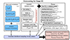 |
Fig. 7. Sketch of the forecasting steps and choices for the stage III configuration. |
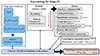 |
Fig. 8. Sketch of the forecasting steps and choices for the stage IV configuration. We explored fewer redshift nuisance models here than for the stage III configurations, since the n(z) biases described in Sect. 3.2.1 are comparatively simple, only featuring shifts in the tomographic mean redshifts that ought to be well compensated for by the δzi model. In addition, results from stage IV forecasts are always considered on the σ8 − Ωm plane given that cosmic shear alone has sufficient constraining power to alleviate the non-linear degeneracy seen for stage III. |
Large-scale structure analysis forecast configurations.
Each forecast was performed as follows. First, the mock data-vector, d, was constructed using the fiducial cosmological and nuisance parameters, given in Table 3, and the true redshift distribution. In our stage III set-up, this true redshift distribution was selected to be one of the mean N(z), unbiased nunb.(z), incoherently biased ni − bias(z), or coherently biased nc − bias(z) distributions described in Sect. 3.1.1. In our stage IV set-up, the true redshift distribution is either the tomographically binned distribution given by Eq. (3.3), or the ‘shifted’ distribution described in Sect. 3.2.1.
Fiducial model parameters.
Given the cosmological model, the distribution of galaxies in redshift, n(z), were converted into a distribution of galaxies in co-moving distance, n(χ) = n(z) dz/dχ, and lensing efficiencies q(χ) via Eq. (2.5). The emulated matter power spectrum, Pδ(k, χ), was integrated over auto-/cross-products of n(χ) and q(χ) (multiplied by fK−2(χ)) to produce the full set of ‘raw’ spectra, Cαβ(ℓ), required by the configuration. These were initially evaluated at eight logarithmically spaced angular wavenumbers, ℓ ∈ [100, 1500], each rounded to the nearest integer. Linear scaling factors,  (Fig. 1; described in Sects. 2.1 and 2.4), were applied to produce the spectral contributions, GG, GI, IG, II, gg, mg, gm, mm, gG, gI, mG, and mI (Sect. 2.1), which were then appropriately summed to produce the ‘observed’ (single) cosmic shear Cγγ(ℓ), (up to two) GGL Cnγ(ℓ), and (up to three) galaxy clustering Cnn(ℓ) angular power spectra.
Next, to mimic real analyses that avoid describing non-linear structure growth with insufficiently complex models, we applied further scale cuts to the clustering and GGL spectra to exclude small physical scales. For each tomographic density sample, nα(z), the maximum angular wavenumber, ℓmax, was calculated as (Mandelbaum et al. 2018)
 (4.1)
(4.1)
where  , and χ(⟨z⟩) is the co-moving distance to the mean of the distribution nα(z). For clustering correlations that have two different density kernels, ℓmax was taken as the minimum of the two. In the case of cosmic shear, we applied no further scale cuts beyond the initial restricted range in ℓ, following KiDS-1000 (Joachimi et al. 2021; Asgari et al. 2021; Heymans et al. 2021). For cosmic shear, this implies ℓmax = 1500.
The final data-vectors are thus formed of ≤6 unique angular power spectra, C(ℓ), defined within and between photometric (shear + density) and spectroscopic (density) samples, including all tomographic auto- and cross-correlations that satisfy the scale cuts described above. Analytic Gaussian covariances are computed for the data-vectors as described in Sect. 2.5, and the data-vector d and inverse data covariance Z are then fixed for the remainder of each forecast.
Some example tomographic power spectra (except the spectroscopic auto-clustering) from a stage III 6 × 2 pt data-vector are given in Fig. 9, which shows the C(ℓ)’s computed for the ‘estimated’ N(z) in black, with error-bars corresponding to the root-diagonal of the Gaussian covariance (for which the corresponding correlation matrix is shown in Fig. 10). Additional curves in Fig. 9 illustrate the thesis of this work: correlations that use the photometric (i.e. the shear) sample as a density tracer (middle top, top right, and bottom left panels) are highly sensitive to changes in the redshift distribution and this information could be used to aid with recalibration of the distribution. This is particularly true of the spectroscopic-photometric cross-clustering, where the spectroscopic n(z) (taken to be exactly known) can act as an anchor for the parameters of any nuisance model – though only if the data are capable of constraining spectroscopic and photometric galaxy biases simultaneously with n(z) model parameters. The cross-clustering is thus only useful in conjunction with both auto-clustering correlations, each quadratically dependent upon its respective galaxy bias (indeed, an all-clustering 3 × 2 pt analysis could be an interesting avenue for exploration). Upon including cosmic shear correlations, both types of GGL correlation then become useful to constrain galaxy intrinsic alignment model contributions (Joachimi et al. 2011), and we arrive at the full 6 × 2 pt analysis.
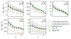 |
Fig. 9. Illustration of tomographic two-point correlations that form a subset of the 6 × 2 pt data/theory-vectors employed in this work. Annotations in the top right of each panel give the spectrum type and tomographic sample pairing, for cosmic shear (γγ), photometric auto-clustering (nPnP), photometric GGL (nPγ), spectroscopic-photometric cross-galaxy-galaxy lensing (nSγ), and spectroscopic-photometric cross-clustering (nSnP) correlations. No spectroscopic auto-clustering correlations are shown, as they are independent of the photometric redshift distribution. Black points and errors give the correlations (Sect. 2.1) and root-diagonal of the Gaussian covariance (Sect. 2.5) computed for the ‘mean’ redshift distribution N(z) (taken as the public estimate from KiDS+VIKING-450; Hildebrandt et al. 2020; Wright et al. 2019 – see Sect. 3.1.1). Coloured curves then show the same correlations, now computed for different redshift distributions: ‘unbiased’ (green, with shading indicating a ±1σ shift in the S8 parameter, holding all else constant); ‘incoherently biased’ (dash-dotted orange); and ‘coherently biased’ (dashed purple). The differences between these curves reflect the sensitivity – to the n(z) and to S8 – of the additional observables that we propose to employ for enhanced internal recalibration of photometric redshift distributions via nuisance models. We note that the positions of coloured curves relative to black points change as a function of redshift pairings across each angular power spectrum, and we are only showing a subset here. |
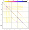 |
Fig. 10. Matrix of correlation coefficients corresponding to an analytical Gaussian covariance, Z (Sect. 2.5), estimated for a (scale-cut; see Sect. 4) stage III 6 × 2 pt data-vector employed in this work. Axis labels denote sections of the covariance corresponding to cosmic shear (γγ), photometric auto-clustering (nPnP), photometric GGL (nPγ), spectroscopic-photometric cross-galaxy-galaxy lensing (nSγ), spectroscopic-photometric cross-clustering (nSnP), and spectroscopic auto-clustering (nSnS) correlations. The sample statistics used for data-vector covariance estimations are those given in Table 1. |
We turn now to the theory-vectors, μ, which were computed in identical fashion to the data-vectors, d, but for different cosmological and nuisance parameters as part of the inference procedure. For each stage III forecast, the initial redshift distribution for computations of μ is the ‘estimated’ N(z) (Sect. 3.1.1), whilst stage IV forecasts start from the distribution given by Eq. (3.3) (and tomographically binned; Sect. 3.2.1).
For stage III forecast configurations making use of the 𝒩comb or 𝒩comb + δzi models (Sect. 2.3)9, we performed an additional set of steps prior to Monte Carlo sampling. First, the comb model was fitted to the initial distribution N(z) by minimization of Eq. (2.22) via the Gaussian-component amplitudes, amμ = ln(Amμ) (see Eqs. (2.19) and (2.20)). The resulting initial ncomb, ini(z) was then used to compute a theory-vector at the fiducial cosmology10 and calculate the goodness of fit, χd2, with respect to the data-vector given the inverse of the signal covariance, Z (Eq. (2.23)). We now varied the comb amplitudes, amμ, again to minimize χd2, leveraging information from the ‘observed’ two-point functions (which correspond to the true redshift distributions) to find the optimized comb model, ncomb, opt(z)11.
The results of this procedure for the forecast configuration  can be seen in Fig. 11. This figure shows the errors in the redshift distributions,
  , and the lensing efficiencies,
  (see Eq. (2.5)), for bins 1 and 3 of the stage III photometric sample after the application of no nuisance model (N(z); dashed purple), of the shift model δzi (dotted red), and of the comb model optimization (solid green). Whilst the correct shift model can provide a reasonably effective correction to the lensing efficiency at higher redshifts, it is clearly seen to add little to the low-redshift bin. It is moreover seen to be generally detrimental to the shape of the n(z), particularly at low redshifts where the z = 0 boundary can cause a large diversion of power towards the tails upon renormalization of the distribution. This is to say that a full-shape bias in the redshift distribution is smoothed out at the level of the lensing efficiency, and perhaps amenable to correction with a scalar shift; however, the same shift is likely to exacerbate the bias at the level of the density distribution. Meanwhile, the optimized comb model is seen to outperform the shift model both in recovering the true lensing efficiency, and in dealing minimal damage to the density distribution, irrespective of the redshift.
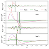 |
Fig. 11. Illustration of the application of redshift nuisance models to the first and third bins of the |


For comb model configurations, the optimized comb ncomb, opt(z) now takes the place of the initial redshift distribution N(z). In the case of the 𝒩comb + δzi model, which applies scalar shifts to ncomb, opt(z) during sampling, we apply Gaussian priors to the shifts with the same widths as inferred from the ensemble {n(z)}X, but now centred on zero. This choice to re-centre the priors is made because the ‘correct’ shift will have changed after optimization of the comb model. Whilst we are able to simply recompute the correct shift here (and we do, for plotting purposes), this information is inaccessible to a real analysis where the true redshift distribution is unknown. Moreover, the 𝒩comb + δzi model uses shifts more to marginalize over n(z) uncertainty than as a corrective measure. Hence, we limited the freedom of shifts during sampling to preserve a fair comparison with the shift model, and we explored the sensitivity of 𝒩comb + δzi constraints to this re-centring by doubling, trebling, and flattening the shift priors, finding some variability in the resultant maxima a posteriori (MAPs) for shift and cosmological parameters (to be discussed in more detail in Sect. 5.3). We note that more complex marginalization schemes (e.g. Stölzner et al. 2021; Cordero et al. 2022) will be explored in future work. In parallel, other promising marginalization techniques for systematics (of and beyond photometric redshifts) are emerging which can significantly speed up the sampling of the likelihood (Ruiz-Zapatero et al. 2023; Hadzhiyska et al. 2023).
We were now ready to sample the posterior probability distribution of cosmological and nuisance parameters under our various probe sets, redshift bias, and redshift nuisance modelconfigurations, as we sought to quantify the advantages of using spectroscopic-photometric cross-correlations to aid with redshift recalibration and reduce cosmological parameter biases. We made use of the nested sampling algorithm, MultiNest (Feroz & Hobson 2008; Feroz et al. 2009, 2019), with the priors given in Table 3, and the following settings:
-
Maximum iterations: 1e5 (S-III), 2e5 (S-IV);
-
N live points: 1e3;
-
efficiency: 0.3;
-
constant efficiency: False;
-
tolerance: 0.01.
For the shift and 𝒩comb + δzi models, the redshift distribution was shifted at each sampling step according to Eq. (2.17), prior to computation of C(ℓ) and evaluation of the log-likelihood, ℒ = −χd2/2 (Eq. (2.23)), whilst it remained fixed for the 𝒩comb and ‘do nothing’ models (Table 2). All other modelling choices were held constant across all forecasts; the differences we explore here are purely due to the interaction of the probes under analysis, and the biases and modelling of redshift distributions.
Assessments of the recovery of point estimates for cosmological parameters are complicated by projection effects (Tröster et al. 2021), and by the variability of estimation by different methods; for example, global MAPs, marginal posterior means, or marginal posterior peaks (Dark Energy Survey and Kilo-Degree Survey Collaboration 2023). Here, we quote posterior means, and compare the results of each forecast with the equivalent results for the respective idealized case; exactly zero redshift bias ( ), and no applied nuisance model (‘do nothing’). We also make estimates of the global MAP parameters for each forecast, starting the Nelder-Mead (Nelder & Mead 1965) algorithm from the fiducial parameter set in order to avoid local minima in the parameter space. We thus verify that the MAP remains at the fiducial parameter set for idealized cases, and observe varying degrees of bias in the best-fit model for all other cases.
We present our findings in the following section, focusing for stage III on the accuracy and precision of recovery of the S8 parameter by cosmic shear alone, and the S8 − Ωm plane for other probe combinations. This is done to reflect the fact that stage III cosmic shear constraints on Ωm are typically prior-dominated (e.g. Joudaki et al. 2017a, 2020). For S8 alone, we quote the mean parameter, and the interval σ68; the difference between the weighted 0.16 and 0.84 quantiles of the posterior distribution. One-dimensional biases on S8 (relative to the idealized case) are then given in ratio to 2σ68. For S8 − Ωm, we quote the figure of merit (FoM), and the two-dimensional parameter bias was calculated according to
 (4.2)
(4.2)
where hats indicate the estimated statistic; unmarked parameters represent the target parameter values (those found by the idealized case); CS8, Ωm denotes the covariance matrix of S8 and Ωm as computed from the weighted chains; and we converted the deviance criterion, χS8 − Ωm2, first into a p value, assuming a χ2 distribution with two degrees of freedom, and then into a significance given in units of σ. The FoM is computed as  .
.
For our stage IV-like forecasts, we found that the typical non-linear ‘banana’ degeneracy on the σ8 − Ωm plane is no longer present, even for cosmic shear alone. We therefore switch to σ8 − Ωm statistics when discussing all stage IV results, which were computed simply by swapping σ8 in for S8 in the above parameter bias (Eq. (4.2)) and FoM formulae.
5. Results
We summarise the results of our stage III forecasts in Table 4, which gives for each {probes : n(z) bias : n(z) model} configuration; the S/N of the data-vector, calculated as a χ2 against a null signal hypothesis; the best-fit χ2 at the global MAP (Eq. (2.23)); and either the S8 parameter bias and the inverse uncertainty 1/σ68 on S8 (for γγ), or the parameter bias (Eq. (4.2)) and the FoM on the S8 − Ωm plane (for all other probe combinations).
Summary statistics for stage III forecasts.
We first consider the stage III scenario in which the n(z) bias is exactly zero, and no redshift nuisance model is marginalized over (bold rows in Table 4). The 1σ confidence contours are shown in Fig. 12 for the primary cosmological parameters constrained by weak lensing: S8, Ωm, σ8, where  and σ8 is derived from the z = 0 linear power spectrum, emulated by CosmoPower using the primordial amplitude ln(1010As) (also shown).
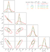 |
Fig. 12. 1σ confidence contours for cosmological structure parameters Ωm, σ8, S8, and ln(1010As), constrained by the forecast configurations having no redshift bias (Table 2; ‘exactly zero’) and applying no nuisance model to the redshift distributions (Table 2; ‘do nothing’). Red contours and curves give the shear-only constraints (γγ); dash-dotted blue the spectroscopic 3 × 2 pt; dashed green the photometric 3ph × 2 pt; and orange the full 6 × 2 pt. Dashed black lines indicate the fiducial parameter centres (Table 3). marginalized posterior probability distributions are seen to extend away from the fiducial centres due to projection effects (discussed in Sect. 5), particularly in the case of ln(1010As). |
While the fiducial centres (Table 3) are recovered by all configurations, the majority of the marginalized posterior volume for ln(1010As) extends away from the MAP towards lower values. Meanwhile, the posterior PDFs of late-time structure growth parameters σ8 and S8 are more centred upon the fiducial values. These are projection effects, where marginalization over the constrained variables results in a preference for low As, which is not constrained by late-time LSS probes (see Tröster et al. 2021, who showed that fixing As during sampling of S8 does not result in significantly different inferences for S8 in the case of KiDS-1000, and also Joudaki et al. 2017a, 2020; Joachimi et al. 2021; Longley et al. 2023 for a discussion of As priors). We moved forwards considering only the constrained cosmological parameters.
The figure legend reports the inverse error on S8 (for γγ only; solid red) or the FoM on the S8 − Ωm plane for all other sets of stage III probe combinations: spectroscopic 3 × 2 pt (dash-dotted blue); photometric 3 × 2 pt (3ph × 2 pt; dashed green); and 6 × 2 pt (solid orange). In this set-up, our shear-only FoM is ∼30% larger than that found by Asgari et al. (2021) because we do not marginalize over redshift nuisance parameters. We have verified that our pipeline is able to reproduce the best-fit parameters and posterior distribution of Asgari et al. (2021) to sub-percent accuracy when analysis choices (including the data-vector and covariance) are homogenized.
In ratio to the idealized 3 × 2 pt configuration, the FoM for the 3ph × 2 pt configuration is ∼5% smaller. While the photometric density tracer is deeper and has fewer galaxy biases to constrain than the spectroscopic sample, it covers only ∼1/12 of the area. For the 6 × 2 pt configuration, the FoM is ∼1.4 times larger (see Table 4).
For the unbiased redshift distribution  without any nuisance model, we begin to see slight biases on the S8 − Ωm plane relative to the idealized cases. These increase in size for the 3ph × 2 pt and 6 × 2 pt configurations – those which use the photometric sample as a density tracer – by up to ∼0.5σ depending on the probes/nuisance model (Table 4). The FoMs are almost unchanged with respect to the idealized scenarios given in Fig. 12. For both the 3ph × 2 pt and 6 × 2 pt configurations, we find weak correlations between the amplitude of intrinsic alignments A1 and the primary cosmological parameters Ωm, S8, σ8.
Not shown are the dimensionless Hubble parameter, h, primordial spectral tilt, ns, and HMCode2016 halo mass-concentration relation amplitude, Abary, as these are only weakly constrained in most configurations. The 6 × 2 pt configuration is the exception, where h approaches a 1σ error of ∼0.02 and ns begins to avoid the boundaries of the prior volume. For next-generation experiments, the 6 × 2 pt configuration could offer more competitive constraints on these variables.
5.1. No nuisance model
We first consider forecasts where we attempt no recalibration of the biased redshift distribution of the photometric sample (the ‘do nothing’ model; Table 2). In Fig. 13, we display 1σ confidence contours for both the incoherently biased case ( , dashed contours) and the coherently biased case (
 , solid contours). Colours denote the same probe sets as in Fig. 12. We recall that our biased redshift distributions (Fig. 4; coloured curves) modify the target data-vector, and that the starting distribution informing the theory-vector is N(z) (black curves in Fig. 4). In Fig. 13 (and subsequent contour figures) we isolate errors in cosmological inference arising from redshift biases, as opposed to projection effects, by quoting parameter biases relative to those observed for the corresponding idealized case; the
  case given in Fig. 12, for which the target distribution
  is identical to the starting distribution N(z).
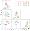 |
Fig. 13. 1σ confidence contours for cosmological structure parameters Ωm, σ8, S8, and the intrinsic alignment amplitude A1, constrained by the γγ, 3 × 2 pt, 3ph × 2 pt, and 6 × 2 pt forecast configurations with ‘incoherently’ (dashed contours and curves) and ‘coherently’ (solid contours and curves) biased redshift distributions, and no nuisance model (‘do nothing’) for redshift recalibration (see Table 2 for a summary of forecast configurations). Colours here denote probe configurations as in Fig. 12 (also given by the legend), whilst line styles denote the type of redshift bias (as described in Sect. 3.1.1). Dashed black cross-hairs display the fiducial, true parameter values. The legend gives for each contour set: the probe combination; the true redshift distribution (i.e. the type of redshift bias); the n(z) nuisance model (given as ‘×’ here, for the ‘do nothing’ model); the FoM on the S8 − Ωm plane (Sect. 4); and the parameter bias in the same plane (comparing posterior means to their equivalents for the |

For several of these forecasts, we see significant biases on the S8 − Ωm plane when failing to recalibrate the biased redshift distributions. The coherent redshift bias manifests more strongly on the S8 − Ωm plane than the incoherent bias – with the exception of 3ph × 2 pt, where the biases are similar. This is due to an increased dependence upon the full shape of the redshift distribution for 3ph × 2 pt and 6 × 2 pt, where the former derives a large proportion of its constraining power from photometric auto-clustering. The incoherently biased distribution  features the largest overall deviation in the full shape (as reckoned by Δfull; Eq. (3.2)), and results in a more significant bias on the S8 − Ωm plane for the 3ph × 2 pt configuration.
The amplitude of intrinsic alignments, A1, is significantly under-estimated by all probe configurations, for each of the two redshift biases. The IA model thus compensates for the redshift errors (van Uitert et al. 2018; Li et al. 2021; Fischbacher et al. 2023). The under-estimation of A1 has the net effect of limiting the GI suppression of the shear signal. The inferred shear signal is therefore asymmetrically boosted, mimicking the shift of lower-z distributions to higher redshifts seen in the upper panels of Fig. 4. For consistency, we have separately verified that in a shear-only case where the redshift distributions are coherently biased towards lower redshifts, the A1 amplitude is correspondingly biased high.
The shear-only (Fig. 13; red contours) and spectroscopic 3 × 2 pt (blue contours) configurations are the most robust to redshift errors, as might be expected given their reliance upon the photometric redshift distribution only at the level of the lensing efficiency q(χ). The shear-only configuration remains biased at just {incoherent: −0.29σ, coherent:0.32σ} in S8. Extending to 3 × 2 pt, the unaffected spectroscopic clustering anchors the σ8 (and thus Ωm) constraints (left panels), yielding biases at {incoherent: 0.07σ, coherent: 0.35σ} on the S8 − Ωm plane.
Both the 3ph × 2 pt (green contours) and 6 × 2 pt (orange contours) configurations show substantial biases on the S8 − Ωm plane. These derive from over-estimations of both S8 and Ωm in the coherent cases (3ph × 2 pt : 2.21σ, 6 × 2 pt : 2.05σ). In the incoherent cases, they derive from (over-) under-estimation of (Ωm) S8 for the 3ph × 2 pt (2.36σ) configuration, and over-estimation of Ωm for the 6 × 2 pt configuration (1.01σ). These results demonstrate the sensitivity of photometric density probes to unmitigated full-shape errors in the redshift distribution.
The inability of the 3ph × 2 pt to constrain Ωm, and hints of bimodality in the posterior (Fig. 13; top left panel, green curves), conspire to degrade the FoM by ∼20 − 30% relative to the 3 × 2 pt configuration, whilst the 6 × 2 pt configurations gain more than 40% in each of the (in)coherent bias cases.
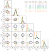 |
Fig. 15. 1σ confidence contours for cosmological and nuisance parameters, as in Fig. 13, now for forecasts employing the shift model for internal redshift recalibration (Sect. 2.1) – we thus include contours for the first, third, and fifth scalar shifts, δzi, and exclude the power spectrum normalization, σ8, in the figure for increased visibility. We show here the difference δp = p − pideal for parameter p relative to the idealized ( |

Fig. 14 displays the one-dimensional posterior means and σ68 intervals for various cosmological and nuisance parameters (rows), relative to the idealized ( ) case for each probe set. Columns give the three redshift bias scenarios (titles), with the four groups of points in each panel corresponding to the applied redshift nuisance models (x axis labels), and colours and line-styles denoting the same probe configurations as in Fig. 12 (also given in legend).
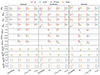 |
Fig. 14. Marginalized one-dimensional constraints for cosmological and (a selection of) nuisance parameters, found by each of our stage III forecast configurations: γγ, 3 × 2 pt, 3ph × 2 pt, and 6 × 2 pt, with colours and line-styles as in Fig. 12 (also given in the legend). The three columns give the unbiased, incoherently biased, and coherently biased forecasts, respectively, and points are grouped on the x axis according to the nuisance model employed by each forecast (see Table 2 for a summary of forecast configurations). Error bars illustrate the σ68 interval, within which the posterior means are given as horizontal markers. y-axes then give the difference δp = p − pideal for parameter p relative to the idealized ( |


Under the ‘do nothing’ model (left-most points in the column), the incoherently biased redshift distribution (middle column), without recalibration, causes the 3ph × 2 pt and 6 × 2 pt configurations to under-estimate σ8 and over-estimate Ωm. This is a consequence of the biased correlations, a subset of which are shown in Fig. 9. For the lower redshift bins, where  is most deviant from N(z) (Fig. 4), photometric clustering statistics typically demand a lower amplitude of correlation to match
  (orange curves in Fig. 9), such that either σ8 or the galaxy bias,
  , must decrease.
Because the shear sample is pushed to higher redshift, this is compensated for in the GGL statistics by an increase in  . σ8 must decrease to satisfy the clustering, whilst
  must increase to satisfy the GGL, and Ωm is forced high (and A1 low) in order to maintain the shear correlation amplitude. This results in a bias on the S8 − Ωm plane, and over-estimations of the galaxy bias, both photometric and spectroscopic, to compensate for the reduced σ8. In the case of the 3ph × 2 pt configuration, the photometric galaxy bias is not anchored by cross-correlations with spectroscopic samples; larger increases in
  force σ8 even lower, and result in an under-estimation of S8. For the 6 × 2 pt configuration, the cross-correlations forbid such large values for the photometric galaxy bias; decreases in σ8 are limited, and S8 remains unbiased.
In the coherent bias scenario, the redshift distributions are similar to those of the incoherent bias for the first two tomographic bins but are then shifted more significantly for the last three bins (Fig. 4). As a result, the coherently biased data-vector requires higher shear correlation amplitudes at intermediate-to-high redshifts, due to the significant offsets in the tomographic means. In this scenario, a severely under-estimated alignment amplitude A1 is unable to provide a sufficient boost to the higher-z correlations (which dominate the cosmic shear S/N). S8 must assume a higher value in order to describe the high-z shear correlations and the S8 − Ωm bias is increased relative to the incoherent case.
These forecasts demonstrate that, when left untreated, different types of errors in redshift calibration can cause the inference of cosmological parameters to be variably biased according to different combinations of weak lensing and density probes. Parameter constraints from configurations using the biased n(z) only for shear statistics (cosmic shear and spectroscopic 3 × 2 pt) are less sensitive to incoherent shifting of redshift distributions, whilst those making use of the same n(z) for density statistics can suffer large errors in the inference of σ8, Ωm, and bg.
In the shear-only, 3 × 2 pt, and 6 × 2 pt incoherently biased cases, we find that S8 remains relatively unbiased, but that this results from the IA model compensating for the redshift uncertainties. While this may be specific to our choice of a biased redshift distribution, Leonard et al. (2024) have found similar results for the 3 × 2 pt in their analysis. If the mean redshift offsets (Fig. 4; vertical orange lines) were not decreasing with redshift (i.e. were not primarily manifested in the first two tomographic bins, in contrast to the coherent bias case, which shifts the mean in every bin), then the resulting errors in shear two-point functions would possibly be less amenable to correction by a modified IA contribution. We now turn to the application of nuisance models that attempt to correct for mis-estimation of galaxy redshift distributions.
5.2. Shift model
We assessed whether or not the shift δzi model – the currently preferred method of redshift distribution recalibration in weak lensing analyses (Hikage et al. 2019; Hamana et al. 2020; Asgari et al. 2021; Amon et al. 2022; Secco et al. 2022) – is sufficient to correct redshift biases in our stage III forecasts (stage IV δzi forecasts are discussed in Sect. 5.4). The parameter contours are displayed in Fig. 15 for both biased redshift scenarios. This includes Ωm, S8, and A1, as previously, along with a subset of the shift parameters δzi.
There is a reduction in bias on the S8 − Ωm plane (and in S8 alone) in all of the δzi forecasts relative to the ‘do nothing’ model. Despite the concerns highlighted in Sect. 4 & Fig. 11, the shift model is unlikely to significantly worsen the accuracy of the S8 and S8 − Ωm inference – though we also note that our applied Gaussian priors for δzi parameters are optimistic (see Sect. 3.1.1).
As in Sect. 5.1, the coherent redshift bias tends to manifest more strongly in the parameter inference than the incoherent bias. Several non-6 × 2 pt configurations are able to gain in FoM with respect to their ‘do nothing’ model counterparts (Fig. 13 and Table 4), despite marginalizing over five additional parameters. This is due to an interplay between (i) degradation of constraints due to the addition of parameters, and (ii) increased S/N in the shear-sensitive parts of the theory-vector, owing to the application of positive shift parameters (aided by Gaussian priors; Sect. 3.1.1) that increase the mean tomographic redshifts of the photometric sample. For some forecasts (notably the coherently biased γγ and 3ph × 2 pt configurations), this results in significantly increased constraining power. This is reflected in the data-vector S/N (Table 4), which reveals the  data-vector to be far more constraining than corresponding
  and
and  data-vectors for γγ and 3ph × 2 pt. Conversely, for
  configurations, the shifts δzi are close to zero; the application of the shift model only results in reduced constraining power relative to the do nothing cases.
In the case of the shift model, with optimistic priors for parameters δzi (Table 3; Sect. 3.1.1), the resulting theory-vectors are translated to higher redshifts where possible. This releases the pressure on A1, and Figs. 14 & 15 consequently reveal much-improved recoveries of the true alignment amplitude by the γγ and 3 × 2 pt shift model configurations.
However, 3ph × 2 pt (green) and 6 × 2 pt (orange) contours in Fig. 15 begin to reveal the deficiencies of the shift model for configurations depending on photometric density tracers. Where shift parameters δzi are able to effectively mitigate the bias in the tomographic mean redshifts for γγ and 3 × 2 pt configurations (red and blue contours, respectively, in the lower right panels), resulting in S8 and S8 − Ωm biases at ≤0.15σ, they are less able to do so for the 3ph × 2 pt and 6 × 2 pt configurations, yielding biases at ∼0.5σ and ∼0.3σ, respectively.
Figs. 14 & 15 show that, whilst the ‘true shifts’ – the actual differences in tomographic mean redshifts between N(z) and  or
or  – are accurately recovered in the γγ and 3 × 2 pt configurations, they are significantly under-estimated in many cases by the 3ph × 2 pt and in all cases by the 6 × 2 pt configurations, where the latter also constrains the shifts to as much as 4× greater precision (Table 5). As highlighted in Sect. 4 and Fig. 11, the correct shifts help the γγ and 3 × 2 pt configurations by reducing the error in the lensing efficiency q(z), but they amplify errors in the full-shape redshift distribution n(z). The shift model therefore has a disproportionately negative impact upon density statistics – principally the photometric clustering – that are sensitive not only to the mean but also to the shape of the redshift distributions.
The 3ph × 2 pt configuration is able to use the shifts to fit higher amplitudes from shear correlations (particularly at at high-z), yielding minor improvements to the recovery of A1 (relative to the ‘do nothing’ case), and a sharp increase in FoM. However, these shifts cause a strong suppression of the density statistics, resulting in an increase in σ8 (coupled to a decrease in bg; Fig. 14), and (to maintain the shear amplitude) a decrease in Ωm. These changes are so large for the  case, that the signs of biases in σ8, Ωm, and bg are flipped relative to the ‘do nothing’ case (Fig. 14).
Meanwhile, the 6 × 2 pt configuration cannot use the shift model to improve the fit to the shear correlations because the spectroscopic-photometric cross-clustering would then be poorly described. It continues to underestimate A1 and remains largely unbiased on the S8 − Ωm plane for both  and
and  – but at the cost of some 11 − 13% of its FoM.
We further elucidate these trends by considering the redshift distribution bias metrics defined in Sect. 3.1.1, Δincoherent and Δfull, now computed for the final redshift distributions with best-fit nuisance models applied (the trends derived for Δincoherent, Δcoherent are quite similar, hence we focus only on Δincoherent here). The left and middle panels in Fig. 16 show for our stage III forecasts the inverse σ68(S8) and FoM on the S8 − Ωm plane vs. the respective parameter biases (relative to the idealized case for each respective probe set) according to Eq. (4.2) (for the 2-d bias). The right-hand panel then shows the corresponding final deviation in tomographic mean redshifts Δincoherent vs. the final full-shape deviation Δfull, each normalized to the relevant untreated (‘do nothing’) case.
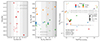 |
Fig. 16. Summary statistics describing the accuracy and precision of the cosmological parameter inference, and corresponding recovery of the true redshift distribution via internal recalibration, for each of our stage III forecast configurations. Colours denote different probe sets, whilst marker-styles give the form of the redshift bias and the applied redshift nuisance model (legends in right panel; star markers denote the |


Marker styles give the nuisance model and redshift bias scenarios as outlined in the middle right and bottom left legends, respectively, whilst colours denote the probe configurations as in previous figures (also given in the top legend). Circular points denote the ‘do nothing’ model, and these are not shown in the right-hand panel, where each would sit at the centre of the cross-hair. Parameter bias thresholds of 0.1σ, 0.2σ, 1σ, 2σ are illustrated in the first two panels with grey shading, such that the unshaded regions indicate higher accuracy of cosmological parameter inference. The precision of parameter inference increases towards the top of these panels. In the right-hand panel, mean redshift ⟨z⟩i errors decrease towards the bottom, whilst full-shape n(z) errors decrease towards the left of the panel.
Each non-circular point in Fig. 16 can be thought of as an attempt to improve upon the corresponding circle (or the cross-hair) via some redshift nuisance model, calibrated by the various two-point data-vectors (denoted by different colours). Whilst the best-fit shift model is able to reduce the cosmological parameter bias in all cases (triangles compared to circles in left and middle panels), it yields a much poorer recovery of the full-shape n(z) (as reckoned by Δfull) when not constrained by the cross-clustering (orange as compared to red, blue, and green triangles; right panel). Under the 6 × 2 pt configurations, which do include the cross-clustering, each shift δzi is constrained to a significantly smaller magnitude at much higher precision. The shift model is thus only able to produce small reductions in Δincoherent and Δfull.
The impact of the best-fit shifts upon the n(z) recoveries can be seen in Fig. 17, where the first two columns show the final redshift distribution error Δn(z) for the stage III (in)coherently biased forecast configurations. In almost every panel, the 6 × 2 pt best-fit shifts yield the closest recovery of the true redshift distribution, followed by the photometric density-probing 3ph × 2 pt, and then the photometric shear-only configurations γγ and 3 × 2 pt. The relative precision of shift parameter constraints is given in Table 5, which quotes σ68 for shifts δzi, for each of the shift model configurations. The 6 × 2 pt probe combination is seen to yield constraints on the shift δzi parameters that are up to ∼4 times more precise (depending on the tomographic bin) than the spectroscopic 3 × 2 pt constraints.
σ68(δzi) for shift parameters δzi.
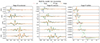 |
Fig. 17. Residual five-bin (rows, 1–5 descending) tomographic redshift distribution errors, Δn(z), found for the best-fit (MAP) shift models (Sect. 2.2) constrained by each of our stage III and stage IV redshift-biased forecasts (see Table 2 for a summary of configurations). Colours and line-styles give the probe configurations as in previous figures (except γγ, indicated here by dotted curves for clarity; see legend). For the stage III configuration, columns show the attempted recoveries of the incoherently (left) and coherently (middle) biased redshift distributions (Sect. 3.1.1), which feature full-shape n(z) deviations. For the stage IV configurations (right), the shifted distribution features pure shifts in the tomographic means (Sect. 3.2.1). The shift model enjoys generally superior recoveries of the true n(z) upon inclusion of spectroscopic-photometric cross-clustering correlations within the 6 × 2 pt configurations. We note that the pure-shift biases examined for the stage IV forecasts are well compensated for (residual errors are at the sub-percent level), and that the shift model offers a comparatively more accurate treatment of these stage IV biases than the full-shape n(z) errors in the stage III forecasts, where the largest residuals exceed 100%. |
The right panel of Fig. 16 demonstrates that, whilst the shift model (triangles) can be effective in mitigating errors in tomographic mean redshifts, it does so at the cost of increased errors in the full shape of the n(z). This is not a problem for probe combinations with weak sensitivity to the n(z) shape, like γγ (red) and 3 × 2 pt (blue), but for configurations probing the photometric density field – 3ph × 2 pt (green) and 6 × 2 pt (orange) – such increases cannot be tolerated. For these configurations, more accurate cosmological inference is achieved through the use of a more flexible nuisance model: the Gaussian ‘comb’ model (squares & diamonds; Sect. 2.3), to which we now turn.
5.3. Comb model
Fig. 18 displays confidence contours for Ωm, S8, A1, δzi, as in Fig. 15, now for the comb + shift (𝒩comb + δzi) model – this model finds an optimized redshift distribution ncomb, opt(z) via Eq. (2.23) before likelihood sampling (see Sects. 2.3 and 4), and then applies the shift model to the optimized n(z) during sampling.
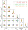 |
Fig. 18. 1σ confidence contours for cosmological nuisance parameters, as in Fig. 15, now for forecasts employing the comb + shift model 𝒩comb + δzi for internal redshift calibration (Sect. 2.3). The comb + shift recalibration reduces biases on the S8 − Ωm plane with respect to the ‘do nothing’ (Fig. 13) and shift (Fig. 15) models, and recovers some of the FoM lost to the shift model even whilst marginalizing over scalar shifts. |
First, considering the S8 − Ωm plane (top left), the (in)coherently biased forecast constraints are almost identical for a given probe configuration, and almost completely unbiased, at ≲0.1σ in most cases. The exception is the 3ph × 2 pt case, where the maximum bias is still relatively small at 0.35σ. This is a significant result, as the data-vectors differ fundamentally between  and
and  , in such ways as to source the various biases found in previous sections, and yet the 𝒩comb + δzi model is able to homogenize the accuracy and precision of the constraints (as is the 𝒩comb model, not shown).
This mitigation of redshift bias is effective regardless of the probe configuration. As seen in the right panel of Fig. 16 for every  and
and  configuration (large squares and diamonds), the comb models are able to reduce the error in Δinc, whilst causing minimal damage to Δfull relative to the corresponding shift models (triangles; some of which are unable to significantly improve Δinc, as discussed in the previous section). We reiterate that the shifts are still in place for the 𝒩comb + δzi model (squares), and yet the n(z) recovery is similar to that seen for the 𝒩comb model (diamonds); the gain, therefore, comes almost exclusively from the flexible optimization of the n(z) against the data-vector, and is not predicated upon the inclusion of cross-clustering correlations (though they help to further improve the recovery). This is also reflected in the final redshift distributions; our analysis of the best-fit 𝒩comb + δzi and pure 𝒩comb models shows smaller Δn(z) performance differentials between the 6 × 2 pt and less complex configurations.
We find some differences in the constraints according to the form of the redshift bias. First, A1 is still slightly under-estimated by the  configuration (at ∼1σ; see the third group of points in the right panel of Fig. 14), though to a lesser extent than for the ‘do nothing’ and δzi models (biased at ≲1.5 − 2σ). This would suggest that the recovery of
  by the optimized comb model is not sufficient to yield large enough shear amplitudes, such that the alignment contribution must continue to compensate.
We further find that the best-fit shifts, δzi, found by the 𝒩comb + δzi configurations are still not equal to the ‘correct’ shifts (recalculated after optimization of the comb to reflect the actual difference in the tomographic mean redshifts), now also for the coherently biased 3 × 2 pt and γγ forecasts. Instead, they are uniformly consistent with zero, for all tomographic bins across all forecasts. This is partially due to the application of zero-mean Gaussian priors for the shifts δzi (with the same widths σi carried over from the ensemble {n(z)}X; Sect. 3.1.1). As discussed in Sect. 4, this was done to preserve a fair comparison between the 𝒩comb + δzi model and the shift model (for which priors limit the freedom of δzi) but also because the original centres for the shifts would be inappropriate after optimization of the comb12.
To investigate the sensitivity of 𝒩comb + δzi maxima a posteriori models to the recentring (to zero-mean) of the δzipriors, we experiment with priors of 2× and 3× the width; flat priors between ±3σi; and with no priors (i.e. a pure maximum-likelihood search). We find that the application of zero-mean priors results in stronger reductions of Δincoherent, and smaller biases on the S8 − Ωm plane, in all cases. When the priors are widened or removed, some configurations start to prefer non-zero shifts δzi, but this always results in a larger S8 − Ωm bias, and 6 × 2 pt configurations always prefer post-comb shifts that are consistent with zero. This suggests that widening the priors for shifts in the 𝒩comb + δzi model does not necessarily yield the correct mean redshifts in the end, and that the primary correction occurs during the comb optimization, as previously indicated.
We tested this interpretation by also considering the comb model without shifts, simply fixing the optimized n(z) for use by the sampler. Under most  and
and  configurations, both the 𝒩comb + δzi and 𝒩comb models (squares and diamonds in Fig. 16) see a reduced parameter bias as well as matched or increased precision in comparison with the corresponding shift model (triangles). In addition, the 𝒩comb makes small gains in precision relative to the 𝒩comb + δzi model (squares), whilst not appreciably losing accuracy. The only exceptions are
  and
and  , where the shift model has higher precision, but at the cost of increased parameter bias. Hence, the strong performance of either of the two comb models relative to the shift model reinforces our expectation that a more flexible recalibration of biased redshift distributions is generally preferred.
That said, we identify shortcomings in our implementation of comb models when applied to the unbiased data-vector (corresponding to  ; Sect. 3.1.1), particularly for the 6 × 2 pt configuration. In this case, the resulting redshift distribution poorly recovers
  compared to the shift or ‘do nothing’ models (top right of right panel in Fig. 16), resulting in best-fit parameters that are biased up to ∼0.5σ on the S8 − Ωm plane. As Fig. 11 shows, the optimized comb (solid green curves) outperforms the shift model (dotted red curves) in recovering both the lensing efficiency q(z) and the redshift distribution n(z), but it cannot avoid slightly amplifying the error in n(z) relative to that seen for the unmodified distribution N(z) (dashed purple curves), as the fine structure is effectively smoothed-over by the Gaussian components. When the true distribution is unbiased relative to the starting distribution, this causes both the initial and optimized comb models to significantly worsen the already-small redshift distribution errors Δn(z) – as seen for the small points in top right corner of the right panel in Fig. 16, where Δfull is effectively a sum over the square of Δn(z). Put differently, the redshift-space width of comb components is not sufficiently narrow to capture the intricate structure of the redshift distribution, and the ‘do nothing’ case consequently offers a closer recovery.
A higher-resolution comb model might be more successful in handling very small redshift distribution errors Δn(z), though we note that there may be associated trade-offs to consider; the optimization procedure would probably be more time-consuming, and a higher density of comb components could increase the space of degenerate n(z) solutions for a given data-vector. But this is not a feature of the comb alone: all small symbols in Fig. 16 are located upwards (and many rightwards) of the cross-hair, signifying that the ‘do nothing’ model, that is, N(z) unmodified, offers the best recovery of  in terms of both the mean redshifts and the full shape (as reckoned by our metrics Δincoherent and Δfull).
The requirement for tuning of a flexible redshift distribution model, and the possibility of introducing biases into pristinely calibrated prior distributions, further motivate the need for more flexible n(z) nuisance modelling, and for marginalization over uncertainty in the n(z). Some tuning of the comb resolution (as in Stölzner et al. 2021) is also likely to be necessary.
As was previously discussed (Sect. 2.3), we do not implement an analytic marginalization over the comb model uncertainty (see Stölzner et al. 2021) in this work, owing to development needed for extended analyses, and questions concerning appropriate priors for comb amplitudes – though analytic marginalization is certainly a primary avenue for improvement. Another possibility is the Hyperrank approach of Cordero et al. (2022) (see similar approaches in Hildebrandt et al. 2017 and Zhang et al. 2023), which consistently and efficiently marginalizes over a space of possible redshift distributions (generated through the external calibration procedure; Myles et al. 2021) by rank-ordering them via hyper-parameters (typically defined as functions of the tomographic mean redshifts ⟨z⟩i) which are then sampled-over in the chain. Inspired by this approach, we suggest a complementary strategy making use of the comb, or other flexible n(z) models. Since the data-vector d and corresponding covariance are typically given ultimate authority to arbitrate between possible recalibrations of the n(z), we propose that the data-vector itself be used to generate the n(z) ensemble. Re-sampling d many times, each sample could be used to constrain a flexible n(z) model – for example, the optimized comb model – assuming the best-fit cosmological and nuisance model for the fiducial data-vector. The resulting ensemble of ncomb, opt(z) realizations would then sample the space of redshift distributions preferred by the observational data, which could be efficiently marginalized over during sampling of the cosmological and nuisance model with the Hyperrankmethod.
5.4. Stage IV forecasts
As a final demonstration of the redshift calibration power of spectroscopic-photometric multi-probe analyses, we turn to our stage IV analysis forecasts, the results of which are summarized in Table 6. Our stage IV synthetic samples (Table 1) take the form of five-bin Rubin LSST Y1-like tomography for the photometric sample (Sect. 3.2.1), and DESI-like bright galaxy, ELG, and LRG spectroscopic samples (Sect. 3.2.2). Besides overall increases to survey depths, areas, and number densities, these mock data also feature greater area and redshift overlaps between spectroscopic and photometric samples, in comparison with our stage-III-like samples. We note that the final results are sensitive to these survey characteristics, which ultimately determine the S/Ns of the different probes explored in this analysis.
Summary statistics for stage IV forecasts.
To simulate redshift biases, we simply drew random scalar shifts from five zero-mean Gaussian distributions, with widths increasing as a function of redshift13, and applied these to the fiducial photometric distributions. This simpler model for redshift bias was adopted owing to a lack of n(z) covariance estimates for our stage-IV-like samples, which would have enabled us to follow a similar procedure to that outlined in Sect. 3.1.1. Given that these are not full-shape n(z) biases, which must be expected for real analyses, we note that these forecasts are more optimistic about the performance of the shift model than those performed for stage III surveys.
We sub-divided the spectroscopic sample into 11 partially overlapping tomographic bins of width Δz ≥ 0.2, as described in Sect. 3.2.2, and conduct forecasts for the subset of configurations given in Table 2. These include the exactly known  and shifted
  redshift distributions; the ‘do nothing’ and scalar shift δzi (with optimistic priors; Sect. 3.1.1) nuisance models; and the four probe configurations: γγ, 3 × 2 pt, 3ph × 2 pt, and 6 × 2 pt. Similarly to the stage III survey set-up, we neglected to run stage IV shift model forecasts where the n(z) was exactly zero (
 ).
).
Fig. 19 displays the collated results of our stage IV forecasts, with red contours corresponding to γγ, blue to 3 × 2 pt, green to 3ph × 2 pt, and orange to 6 × 2 pt. Solid contours display ntrue(z) forecasts without any nuisance model; the idealized scenarios. We note that the blue, green, and orange contours are often overlapping. We find that the non-linear σ8 − Ωm degeneracy seen for stage III analyses is linearized for our stage IV set-up, and quote statistics for the σ8 − Ωm plane accordingly. Relative to γγ, the FoM(σ8 − Ωm) is seen to increase by factors of ∼2.7 (3 × 2 pt), ∼2.6 (3ph × 2 pt), and ∼3.1 (6 × 2 pt).
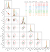 |
Fig. 19. 1σ confidence contours for cosmological and nuisance parameters, as in Fig. 15, now for all forecasts conducted using synthetic stage-IV-like galaxy samples (Sects. 3.2.1 & 3.2.2), including: the true redshift distribution |


Dotted contours give the  forecasts14, also without any nuisance model for the n(z). The induced biases on the σ8 − Ωm plane are seen to be severe. Similar to our stage III forecasts, the alignment amplitude A1 is significantly mis-estimated as a consequence of unmitigated redshift biases. In contrast to the stage III 3ph × 2 pt configurations, A1 is shifted high here due to the different form of redshift bias, with bins 2–4 shifted low, and bins 1 & 5 shifted high. Whilst the net requirement for the γγ and 3 × 2 pt configurations is for increased shear amplitudes, resulting in underestimations of A1 (similarly to stage III), the 3ph × 2 pt must also satisfy a demand for reduction of photometric GGL signals, and thus yields an overestimation of A1.
The dashed contours in Fig. 19 show the  forecasts with the application of the shift model for redshift recalibration. The scalar shifts are found to effectively mitigate the σ8 − Ωm bias for each of the configurations. However, weak δzi constraints and inter-parameter correlations (between δzi, and with A1 and cosmological parameters) cause the γγ, 3 × 2 pt, and 3ph × 2 pt configurations to lose significant proportions of their FoM in exchange for the correction. In contrast, the 6 × 2 pt configuration is able to constrain the shift parameters at up to ∼19×, 6×, and 4× the precision seen for γγ, 3 × 2 pt, and 3ph × 2 pt, respectively (Table 5), thereby retaining > 90% of its idealized FoM. As a result, the FoM(σ8 − Ωm) gain factor, relative to γγ, is ∼7.9 (3 × 2 pt), ∼7.3 (3ph × 2 pt), and ∼14.6 (6 × 2 pt) – the 6 × 2 pt analysis allows for a far-superior retention of constraining power throughout the n(z) recalibration.
We reiterate that the artificial redshift distribution bias implemented for these forecasts is particularly generous to the shift model (see Fig. 17, where the n(z) error is reduced to sub-percent level by each configuration). One should expect the recalibration to suffer in all cases under more realistic redshift calibration errors, such as those implemented in our stage III forecasts (Sect. 3.1.1). However, improved recalibration upon inclusion of cross-clustering correlations should be expected for any form of redshift bias, as demonstrated by the dramatic increases in precision for nuisance parameters constrained by the stage III and stage IV 6 × 2 pt forecasts, independent of the suitability of the model for correction of the bias.
We note here that, as discussed in Sect. 2.2, stage IV forecasts are far more capable of meaningfully constraining the halo model amplitude Abary, when compared with their stage III counterparts – particularly the 6 × 2 pt and 3ph × 2 pt configurations, for which the upper edge of the prior (indicating a zero-feedback universe) sits beyond 4σ in the marginalized 1-d posterior distribution (not shown). Our work therefore indicates that, modulo the approximations made here, the next generation of weak lensing experiments is indeed promising for the future of baryonic feedback modelling.
We acknowledge that stage IV analyses wishing to make use of galaxy clustering and GGL measurements up to our fiducial kmax = 0.3 h Mpc−1 will most likely need to go beyond the linear bias assumption (e.g. Nicola et al. 2024). For this reason, we also considered a scenario where the analysis is restricted to kmax = 0.1 h Mpc−1. We find that this scenario does not remove the biases caused by uncorrected photometric redshifts shifts; they remain comparable to our fiducial scenario. The stricter kmax cut does result in lowered FoM values, as one would expect from including fewer modes in the data vector. However, comparatively, the 6 × 2 pt probe combination is the most robust to the small-scale cuts. This manifests in a factor of ∼3 improvement in the FoM relative to the 3 × 2 pt probe combination, instead of a factor of ∼2 fiducially, which is in line with previous work (Joudaki & Kaplinghat 2012).
5.5. Speed of convergence
We remark here upon the requirements and consequences posed by the inclusion of spectroscopic-photometric cross-clustering correlations within the joint LSS analysis. We emphasize that our conclusions here might be specific to the choice of a nested sampler and the priors adopted in our analyses and they might change if either of these choices are modified.
One of the major lessons learned during this study is that the cross-clustering works to improve nuisance recalibration of redshift distributions by dramatically decreasing acceptance fractions during the sampling of the posterior probability distribution. This reflects the much smaller space of parameters that are able to simultaneously satisfy the cross-clustering – pinned to the spectroscopic n(z) – and the demands from shear correlations for modified redshift distributions.
The time required for convergence of the chains is found to increase accordingly. In order to enable the running of many forecast configurations including the cross-clustering, this motivated us to make the series of approximations described in Sect. 2.4. We illustrate this point in Fig. 20, which shows the likelihood evaluation rates (top), final acceptance fractions (middle), and total run-times15 (bottom) of our stage III forecasts (colours denote probe configurations; see Table 2). Our approximations enabled us to evaluate the likelihoods of extended data-vectors ∼20 times per second, on-average, and yet the low acceptance rate (middle panel; leftward) of the 6 × 2 pt configuration resulted in total run-times ranging from a few days to several days, with the slowest approaching 10 days (40–48 cores). If we are to utilize the redshift calibration power from cross-clustering in future analyses, further advances in the realms of power spectrum emulation and fast computation of other cosmological functions would be a great boon.
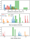 |
Fig. 20. Histograms showing the number of likelihood evaluations per second (top), the final accepted fraction of evaluations (middle), and the total forecast run-time in hours (bottom) of our stage III forecasts, coloured according to the probe configurations (as in previous figures, and also given in the legend; see Table 2). We note that these are indicative estimates for runtimes, excluding some forecasts that were rerun at later stages, and including some variability stemming from the number of parallel threads utilized for each specific forecast. As a result, some forecast timings were unrepresentative (< 10 evaluations s−1), and these are not shown. |
6. Conclusions
We have conducted simulated likelihood forecasts for the fully combined analysis of weak lensing and galaxy clustering from overlapping stage-III- and stage-IV-like photometric and spectroscopic galaxy surveys. In particular, we assessed the potential for positional cross-correlations between the spectroscopic and photometric galaxies to improve the precision and accuracy of the calibration of shear sample redshift distributions, thereby reducing biases in the cosmological parameter inference and increasing the statistical constraining power of the surveys.
Synthetic stage III samples were defined to have similar photometric statistics to the ones reported for the fourth Data Release of the Kilo Degree Survey (Kuijken et al. 2019), supplemented by spectroscopic galaxies from the completed Baryon Oscillation Spectroscopic Survey (Eisenstein et al. 2011) and 2-degree Field Lensing Survey (Blake et al. 2016), assuming 661 deg2 of overlap (Asgari et al. 2021). For our stage IV configuration, we mimicked the expected statistics for the first year of Rubin Observatory: Legacy Survey of Space and Time observations (Mandelbaum et al. 2018), supplemented by spectroscopic observations resembling the Dark Energy Spectroscopic Instrument bright galaxy, ELG, and LRG samples (DESI Collaboration 2016), assuming 4000 deg2 of overlap.
We simulated redshift calibration failures for stage III surveys by sampling many thousands of five-bin redshift distributions with variations over the full n(z) shape and selecting extreme outliers in terms of the differences in tomographic mean redshifts. We distinguished between samples according to the ‘coherence’ of the mean redshift errors; whether the bulk distribution is shifted in one direction, or features more internal scattering and full-shape n(z) errors. Our goal with our choice of n(z) realizations was to find a pessimistic scenario that is still compatible with the structure of the n(z) covariance. Beyond the expected degrees of cosmological parameter bias, we are particularly interested in understanding the capacity of probe combinations to mitigate such extreme n(z) calibration errors. For our stage IV configuration, we simply drew random, uncorrelated shifts to apply to the means of tomographic distributions, making it more closely resemble a stage III ‘incoherent’ bias, but lacking full-shape errors due to the lack of a realistic redshift distribution covariance.
We explored the capabilities of the commonly used tomographic bin-wise shift parameters in recalibrating redshift distributions to accommodate such biases, in contrast to a flexible Gaussian mixture model for the n(z), as well as a ‘do nothing’ case in which the biases were left unaddressed. Our central proposal was that any redshift recalibration model should be more precisely and accurately constrained by analyses that include clustering cross-correlations with spectroscopic samples, thereby ‘pinning’ the nuisance variables to the well-known spectroscopic n(z). To this end, we explored joint analyses of various combinations of up to six cosmological observables, probing the cosmic shear field traced by photometric galaxies and the cosmic density field traced by both photometric and spectroscopic galaxies.
We modelled the matter power spectrum, P(k), with the CosmoPower emulator (Spurio Mancini et al. 2022), trained against a library of power spectra featuring baryonic contributions according to the one-parameter HMCode2016 model (Mead et al. 2015, 2021). We used the CCL library (Chisari et al. 2019a) in ‘calculator’ mode to compute Limber-approximated angular power spectra for the cosmic shear, Cγγ(ℓ), GGL, Cnγ(ℓ), and galaxy clustering, Cnn(ℓ), including all contributions from lensing magnification and intrinsic alignments. We considered the multipole range ℓ ∈ [100, 1500] for a stage III (and ℓ ∈ [100, 3000] for a stage IV) survey set-up, modelling all scales for cosmic shear correlations and limiting positional probes to an ℓmax corresponding to  at a given redshift.
We performed simulations for a flat-ΛCDM cosmological model, sampling the posterior probability distribution for five cosmological parameters, Ωch2, Ωbh2, ln(1010As), h, ns (then deriving σ8 and  ), one amplitude each for intrinsic alignments, A1, and baryonic contributions, Abary, (if applicable) one linear galaxy bias, bg, per tomographic sample, and (if applicable) one scalar shift, δzi, in the mean redshift per photometric tomographic sample. We used an analytical Gaussian covariance in the process. Our primary findings are summarized as follows:
-
Under idealized conditions, without redshift biases or nuisance models, a stage III 6 × 2 pt analysis offers a ∼40% gain in FoM on the S8 − Ωm plane, relative to the spectroscopic 3 × 2 pt analysis, and a ∼45% gain relative to the photometric 3ph × 2 pt analysis (noting these figures may be specific to our sample definitions).
-
The relative coherence of biases in the redshift distribution is important in determining the manifestation of the bias at the level of cosmological parameters. Coherent biases – uni-directional shifts in the bulk distribution – are more likely to affect the determination of S8 by demanding large changes to the shear correlation amplitudes across all redshifts. Conversely, incoherent biases – multi-directional shifts, and full-shape errors – are more harmful to inferences of σ8, Ωm and the photometric galaxy bias,
 , as they manifest more strongly in density correlations that depend differently upon σ8 and Ωm.
 -
If we do nothing to the (either coherently or incoherently) biased redshift distributions, the intrinsic alignment amplitude, A1, is mis-estimated in order to compensate for the redshift errors. Modifications to A1 can suppress or amplify the shear signal (primarily via GI contributions to off-diagonal correlations), and thereby mimic the shifting of lower-z bins. This is less effective at higher redshifts, where intrinsic alignments are weaker, and where most of the S/N for cosmic shear lies. We confirm that the direction of the error in A1 corresponds to the direction of the bias in tomographic mean redshifts; under-estimation of mean redshifts results in an under-estimation of A1, though this picture is complicated when considering multiple probes beyond cosmic shear, or when tomographic mean errors are variable, that is, multi-directional.
-
Even when the IA amplitude is mis-estimated in this way, there remain significant biases on the S8 − Ωm plane, especially for the photometric 3ph × 2 pt (≳2σ) and 6 × 2 pt (≳1σ) configurations. Among all configurations, the spectroscopic 3 × 2 pt is the most robust to redshift biases, owing to its weaker sensitivity to the fine structure of the photometric n(z).
-
The ‘shift model’ is often able to reduce the overall error, Δinc, in the tomographic mean redshifts, but does so whilst typically increasing the full-shape n(z) error, Δfull. Cosmic shear, γγ, and the spectroscopic 3 × 2 pt configuration (with spectroscopic lens galaxies) are sensitive to the photometric redshift distribution only via the lensing efficiency, which is largely determined by the mean redshift; increases to Δfull are relatively unimportant here, and the shift model is effective in mitigating cosmological parameter biases.
-
In contrast, the photometric 3ph × 2 pt and 6 × 2 pt configurations are sensitive to the full shape of the n(z) via photometric density probes. In these cases, significant increases in Δfull cannot be tolerated by the data-vector. The shift model is thus less able to reduce Δinc, such that the n(z) recovery is relatively poor, and small cosmological parameter biases remain, at ∼0.5σ (3ph × 2 pt) and ∼0.3σ (6 × 2 pt).
-
A more flexible model for n(z) recalibration – the ‘comb’, a Gaussian mixture model – is able to effectively mitigate tomographic mean errors, Δinc, without also expanding the full-shape errors, Δfull. With or without the additional application of scalar shifts, this model yields the most accurate recoveries of (in)coherently biased redshift distributions, and lowest cosmological parameter biases, per the configuration of probes. However, more work is needed to ensure that the comb does not yield adverse impacts for near-perfectly calibrated redshift distributions, for which n(z) biases are not significant.
-
For the stage III configuration, the inclusion of spectroscopic-photometric cross-clustering correlations within the full 6 × 2 pt analysis yields up to ∼4× and ∼2× tighter constraints upon shift model parameters δzi, relative to the 3 × 2 pt and 3ph × 2 pt analyses, respectively. For our stage IV set-up, these figures rise to ∼6× and ∼4×, respectively. This gain in nuisance calibration power translates into double the σ8 − Ωm FoM compared to 3 × 2 pt/3ph × 2 pt, and only an ∼8% FoM loss compared to the idealized, zero-bias 6 × 2 pt scenario. Large-scale structure analyses seeking to maximize constraining power whilst effectively mitigating redshift calibration errors should therefore consider making use of cross-clustering correlations for their enhanced recalibration potential.
6.1. Outlook
One of the challenges we expect for the application of this method is the computational cost of the likelihood evaluations. This will be particularly important for stage IV surveys where the modelling will have to be more accurate (and costly) to match the precision of the data. Most of the cost derives from the computation of cross-clustering correlations between spectroscopic and photometric datasets, which enlarge the data-vector but also diminish the fraction of accepted parameter samples that make up the chains. The former could in principle be improved by pre-computation and emulation of the angular power spectra (as opposed to the matter power spectrum), but the latter is likely to pose a consistent challenge. We emphasize that this challenge might be specifically linked to our choice of a nested sampler.
Another aspect to be explored is the configuration of the comb model. In our work, we followed closely the set-up of Stölzner et al. (2021), which applied the methodology to cosmic shear alone. In principle, the addition of clustering and GGL statistics could enable a finer comb to more accurately recover the n(z), which we have found to be desirable for the handling of residual A1 biases or initially unbiased redshift distributions, as is discussed in Sect. 5.3. However, a finer comb incurs additional computational costs in the context of analytic marginalization, where the number of required operations per likelihood evaluation is dramatically increased. For the 𝒩comb + δzi and 𝒩comb approaches explored here, the additional cost would be minimal. The impact of a more motivated marginalization over uncertainty in the comb model remains to be explored for (3−6) × 2 pt analysis configurations. This could be achieved following the methodology in Stölzner et al. (2021) or by incorporating a strategy more similar to Hyperrank (see Cordero et al. 2022, and the discussion at end of Sect. 5.3). Ideally, we would also explore more variably biased redshift distributions; the coherent and incoherent cases could be more dissimilar, with a different net direction of bias, and a distribution maximizing the full-shape error (as opposed to the error in the means) would be of interest.
The need for fast theory-vector evaluations in order to run our full likelihood analyses of the 6 × 2 pt correlations has led us to make some simplified model choices. Although we acknowledge that the accuracy needs of next-generation data require more complex LSS modelling, we emphasize that the choices were homogeneous throughout the different probe combinations, (3−6) × 2 pt. This allowed us to make meaningful comparisons between them. However, in the future, it will be important to enable extensions of our pipeline to include more accurate models of baryons (van Daalen et al. 2011, 2020; Chisari et al. 2019b; Mead et al. 2021; Salcido et al. 2023), intrinsic alignments (Blazek et al. 2019; Vlah et al. 2020; Fortuna et al. 2021; Bakx et al. 2023; Maion et al. 2024), redshift space distortions (Kaiser 1987; Taylor & Hamilton 1996; Ross et al. 2011), non-Limber angular power spectra (Campagne et al. 2017; Fang et al. 2020; Leonard et al. 2023), non-linear bias (Baldauf et al. 2011; Pandey et al. 2020; Mead et al. 2021; Nicola et al. 2024), and fingers-of-God (Jackson 1972), and of their redshift evolution. The increased constraining power of the 6 × 2 pt configuration also makes it interesting to open up the cosmological parameter space, and to determine the constraining power of this probe combination in terms of curvature, neutrino mass, evolving dark energy, and other extensions (Joudaki et al. 2017b; Tröster et al. 2021; Abbott et al. 2023; Adame et al. 2025).
In this work, we have fixed the number of spectroscopic sample redshift bins (for each stage). It would be useful for future work to explore whether or not fewer bins could achieve the same performance in recalibrating the photometric redshifts of the shear sample, whilst reducing the cost of each likelihood evaluation.
As the main motivation of this work has been to understand the gains from including spectroscopic-photometric cross-correlations, we decided to work with projected angular power spectra of the clustering of these galaxies instead of their three-dimensional power spectra. In the future, this alternative could also be explored. This would increase the cosmological constraining power in the spectroscopic sample alone (e.g. Joudaki et al. 2018; Heymans et al. 2021), specifically by breaking degeneracies with Ωm and the spectroscopic bias parameters (through the redshift space distortions; Kaiser 1987). The challenge lies in computing and validating the covariance matrix when the estimators used for the different tracers are not the same, which has thus far been achieved by creating a large suite of numerical simulations (Harnois-Déraps & van Waerbeke 2015; Joachimi et al. 2021; Joudaki et al. 2018; Heymans et al. 2021). Recent work moreover suggests a possible avenue for its analytic computation (Taylor & Markovič 2022).
We have considered the same, linear galaxy bias function for the spectroscopic and photometric samples. It is likely that the galaxy bias will differ in the real data due to the differences in the redshift coverage and depth of each sample. This can have advantages in terms of cosmological constraints, as differently biased tracers that sample the same underlying field can mitigate the impact of cosmic variance on the cosmological constraints (McDonald & Seljak 2009).
The increased constraining power from the 6 × 2 pt probe combination results in a higher sensitivity to modelling choices. Each element of the model should be tested in the future, such as whether the 6 × 2 pt analysis is sensitive to models of intrinsic alignments with higher complexity than NLA, or to fundamental parameters such as neutrino mass (Font-Ribera et al. 2014). In this work, except for the case of photometric redshift distributions, we have always matched the model in the synthetic data vector with that in the theoretical prediction, but these can be deliberately mismatched to assess potential biases in the cosmological parameters due to assuming overly simplistic models given the precision of the data. The same applies to models of galaxy bias, baryonic feedback, and other astrophysical or instrumental effects. This should further be coupled to an exploration of the range of scales being used in the analysis; for example, ℓmax (e.g. Krause et al. 2016).
Notice that we work here in redshift space, while n(χ) = n(z) dz/dχ, which requires a model for the expansion of the Universe.
We do not make use of the latest version, HMCode2020 (Mead et al. 2021), as it was comparatively less well tested within CosmoPower at the start of our analysis.
CCL version: 2.3.1.dev7+ge9317b4f.
We note here for clarity that the KV450 redshift distribution, denoted N(z), is equal to: (i) the mean of the distribution from which samples n(z) are drawn to simulate photometric redshift biases; (ii) the ‘estimated’, or ‘starting’ distribution for simulated likelihood analyses, to which nuisance models will be applied; and (iii) in limited forecast cases of zero redshift bias, the actual target distribution, denoted  . Meanwhile, n(z) refers to a sample redshift distribution drawn from the covariance, and in later sections to any arbitrary redshift distribution.
This could lead to complications that must be considered if, for example, per-galaxy weights are intended for the mitigation of systematic density fluctuations in measured positional statistics (Rezaie et al. 2020; Wagoner et al. 2021).
Notice that we differentiate between the estimated N(z), the initial guess for the redshift distribution, and n(z), the true distribution informing the data-vector, that is the target distribution.
We neglect quasar (QSO/LyαQSO) samples such as those observed by DESI, so as to lessen the computational demands of these forecasts. Future work could consider these additional, sparser but higher-redshift samples, as well as other spectroscopic observations planned to overlap with stage IV surveys. Note also that observational results now present in data.desi.lbl.gov were not available when this work was in progress.
In comparison to recent DESI Collaboration results (Yu et al. 2025; Krolewski et al. 2025), the redshift success rates we have adopted are either lower or equal. Therefore, the number density of targets we have used for this work is conservative.
We note that whilst the comb model is considered for the stage III forecasts, its use would be excessive for our simple stage IV redshift bias implementation; hence we do not apply it to the stage IV forecasts in this work.
Real analyses will not have access to the fiducial cosmological/nuisance parameter set. As described by Stölzner et al. (2021), this point must be found via an iterative maximum likelihood search, alternating between the spaces of cosmological and nuisance parameters.
We note that the results of optimization of the comb model are sensitive to the choice of minimization algorithm and its hyper-parameters. We homogenize these choices across all forecasts, using the Nelder-Mead (Nelder & Mead 1965) algorithm with a maximum of 30 000 function evaluations, and suggest a more detailed exploration regarding flexible n(z) model parametrization in future work.
One could compute new non-zero centres for the shift priors after comb optimization, but this would involve returning to the hypothetical external redshift calibration. Instead, we assume that the mean correction has been applied by the comb optimization, and proceed with zero-mean priors for the shifts.
The resulting shifts were [0.016, −0.012, −0.016, −0.043, 0.043], respectively.
In this case, we refrain from showing the 6 × 2 pt configuration due to difficulty in finding convergence.
We note that minor timing overheads are incurred by the optimization process for each of our stage III comb model configurations. The magnitude of the overhead is dependent upon the choice of algorithm, its hyperparameters (e.g. tolerance, maximum function evaluations, etc.), and the probes–redshift bias combination. Regardless, the time to optimize is subdominant to that required by likelihood sampling, and the optimization timing is not included in Fig. 20.
Acknowledgments
This paper went through a KiDS internal review process. We are grateful to Markus Michael Rau and Elena Sellentin for helpful discussions, and we also thank Alessio Spurio Mancini for his development of and continued improvements to the CosmoPower emulator, without which this work would not have been possible. We thank members of the KiDS consortium for stimulating discussions and support throughout this work, and the anonymous referee for their helpful comments. HJ, NEC acknowledge support from the Delta ITP consortium, a program of the Netherlands Organisation for Scientific Research (NWO) that is funded by the Dutch Ministry of Education, Culture and Science (OCW), project number 24.001.027. This publication is also part of the project ‘A rising tide: Galaxy intrinsic alignments as a new probe of cosmology and galaxy evolution’ (with project number VI.Vidi.203.011) of the Talent programme Vidi which is (partly) financed by the Dutch Research Council (NWO). SJ acknowledges the Dennis Sciama Fellowship at the University of Portsmouth and the Ramón y Cajal Fellowship from the Spanish Ministry of Science. AL acknowledges support from the research project grant ‘Understanding the Dynamic Universe’ funded by the Knut and Alice Wallenberg Foundation under Dnr KAW 2018.0067. BJ acknowledges support by the ERC-selected UKRI Frontier Research Grant EP/Y03015X/1 and by STFC Consolidated Grant ST/V000780/1. RR, JLvdB and AD are supported by an ERC Consolidator Grant (No. 770935). KK acknowledges support from the Royal Society and Imperial College. BS, ZY and SU acknowledge support from the Max Planck Society and the Alexander von Humboldt Foundation in the framework of the Max Planck-Humboldt Research Award endowed by the Federal Ministry of Education and Research (Germany). TT acknowledges funding from the Swiss National Science Foundation under the Ambizione project PZ00P2_193352. AHW is supported by the Deutsches Zentrum für Luft- und Raumfahrt (DLR), made possible by the Bundesministerium für Wirtschaft und Klimaschutz, and acknowledges funding from the German Science Foundation DFG, via the Collaborative Research Center SFB1491 ‘Cosmic Interacting Matters – From Source to Signal’. HH is supported by a DFG Heisenberg grant (Hi 1495/5-1), the DFG Collaborative Research Center SFB1491, an ERC Consolidator Grant (No. 770935), and the DLR project 50QE2305. MA acknowledges support from the UK Science and Technology Facilities Council (STFC) under grant number ST/Y002652/1 and the Royal Society under grant numbers RGSR2222268 and ICAR1231094. MB is supported by the Polish National Science Center through grants no. 2020/38/E/ST9/00395, 2018/30/E/ST9/00698, 2018/31/G/ST9/03388 and 2020/39/B/ST9/03494. BG acknowledges support from a UK STFC Consolidated Grant and from the Royal Society of Edinburgh through the Saltire Early Career Fellowship (ref. number 1914). CH acknowledges support from the European Research Council under grant number 647112, from the Max Planck Society and the Alexander von Humboldt Foundation in the framework of the Max Planck-Humboldt Research Award endowed by the Federal Ministry of Education and Research, and the UK Science and Technology Facilities Council (STFC) under grant ST/V000594/1. LL is supported by the Austrian Science Fund (FWF) [ESP 357-N]. HYS acknowledges the support from CMS-CSST-2021-A01 and CMS-CSST-2021-A04, NSFC of China under grant 11973070, and Key Research Program of Frontier Sciences, CAS, Grant No. ZDBS-LY-7013 and Program of Shanghai Academic/Technology Research Leader. MWK acknowledges support from the Science and Technology Facilities Council. CM acknowledges support under the grant number PID2021-128338NB-I00 from the Spanish Ministry of Science, and from the European Research Council under grant agreement No. 770935. Part of this work is based upon public data products produced by the KiDS consortium, derived from observations made with ESO Telescopes at the La Silla Paranal Observatory under programme IDs 100.A-0613, 102.A-0047, 179.A-2004, 177.A-3016, 177.A-3017, 177.A-3018, 298.A-5015. Figures in this work were produced using matplotlib (Hunter 2007) and ChainConsumer (Hinton 2016). Author contributions: all authors contributed to the development and writing of this paper. The author list is given in three groups: the lead authors (HJ, NEC, SJ, RR, BS), followed by two alphabetical groups. The first alphabetical group includes those who are key contributors to both the scientific analysis and the data products. The second group covers those who have either made a significant contribution to the data products or the scientific analysis.
References
- Abbott, T. M. C., Abdalla, F. B., Alarcon, A., et al. 2018, Phys. Rev. D, 98, 043526 [NASA ADS] [CrossRef] [Google Scholar]
- Abbott, T. M. C., Aguena, M., Alarcon, A., et al. 2022, Phys. Rev. D, 105, 023520 [CrossRef] [Google Scholar]
- Abbott, T. M. C., Aguena, M., Alarcon, A., et al. 2023, Phys. Rev. D, 107, 083504 [NASA ADS] [CrossRef] [Google Scholar]
- Abdalla, E., Abellán, G. F., Aboubrahim, A., et al. 2022, J. High Energy Astrophys., 34, 49 [NASA ADS] [CrossRef] [Google Scholar]
- Adame, A. G., Aguilar, J., Ahlen, S., et al. 2025, JCAP, 2025, 021 [CrossRef] [Google Scholar]
- Alarcon, A., Sánchez, C., Bernstein, G. M., & Gaztañaga, E. 2020, MNRAS, 498, 2614 [NASA ADS] [CrossRef] [Google Scholar]
- Alonso, D., Sanchez, J., Slosar, A., & LSST Dark Energy Science Collaboration 2019, MNRAS, 484, 4127 [NASA ADS] [CrossRef] [Google Scholar]
- Amon, A., Gruen, D., Troxel, M. A., et al. 2022, Phys. Rev. D, 105, 1 [Google Scholar]
- Asgari, M., Tröster, T., Heymans, C., et al. 2020, A&A, 634, A127 [NASA ADS] [CrossRef] [EDP Sciences] [Google Scholar]
- Asgari, M., Lin, C.-A., Joachimi, B., et al. 2021, A&A, 645, A104 [NASA ADS] [CrossRef] [EDP Sciences] [Google Scholar]
- Awan, H., Gawiser, E., Kurczynski, P., et al. 2016, ApJ, 829, 50 [Google Scholar]
- Ayçoberry, E., Ajani, V., Guinot, A., et al. 2023, A&A, 671, A17 [NASA ADS] [CrossRef] [EDP Sciences] [Google Scholar]
- Bakx, T., Kurita, T., Elisa Chisari, N., Vlah, Z., & Schmidt, F. 2023, JCAP, 2023, 005 [Google Scholar]
- Baldauf, T., Seljak, U., Senatore, L., & Zaldarriaga, M. 2011, JCAP, 2011, 031 [CrossRef] [Google Scholar]
- Barreira, A., Krause, E., & Schmidt, F. 2018a, JCAP, 2018, 015 [Google Scholar]
- Barreira, A., Krause, E., & Schmidt, F. 2018b, JCAP, 2018, 053 [Google Scholar]
- Barreira, A., Lazeyras, T., & Schmidt, F. 2021, JCAP, 2021, 029 [CrossRef] [Google Scholar]
- Bartelmann, M., & Schneider, P. 2001, Phys. Rep., 340, 291 [Google Scholar]
- Bautista, J. E., Paviot, R., Vargas Magaña, M., et al. 2021, MNRAS, 500, 736 [Google Scholar]
- Baxter, E. J., Chang, C., Hearin, A., et al. 2022, ArXiv e-prints [arXiv:2203.06795] [Google Scholar]
- Bernardeau, F., van Waerbeke, L., & Mellier, Y. 1997, A&A, 322, 1 [NASA ADS] [Google Scholar]
- Bernstein, G. M. 2009, ApJ, 695, 652 [NASA ADS] [CrossRef] [Google Scholar]
- Bernstein, G. M., & Cai, Y.-C. 2011, MNRAS, 416, 3009 [Google Scholar]
- Beutler, F., & McDonald, P. 2021, JCAP, 11, 031 [Google Scholar]
- Blake, C., Amon, A., Childress, M., et al. 2016, MNRAS, 462, 4240 [NASA ADS] [CrossRef] [Google Scholar]
- Blanchard, A., Camera, S., Carbone, C., et al. 2020, A&A, 642, A191 [NASA ADS] [CrossRef] [EDP Sciences] [Google Scholar]
- Blazek, J. A., MacCrann, N., Troxel, M. A., & Fang, X. 2019, Phys. Rev. D, 100, 103506 [NASA ADS] [CrossRef] [Google Scholar]
- Bridle, S., & King, L. 2007, New J. Phys., 9, 444 [Google Scholar]
- Cai, Y.-C., & Bernstein, G. 2012, MNRAS, 422, 1045 [Google Scholar]
- Campagne, J. E., Neveu, J., & Plaszczynski, S. 2017, A&A, 602, A72 [NASA ADS] [CrossRef] [EDP Sciences] [Google Scholar]
- Catelan, P., Kamionkowski, M., & Blandford, R. D. 2001, MNRAS, 320, L7 [NASA ADS] [CrossRef] [Google Scholar]
- Chisari, N. E., Alonso, D., Krause, E., et al. 2019a, ApJS, 242, 2 [Google Scholar]
- Chisari, N. E., Mead, A. J., Joudaki, S., et al. 2019b, Open J. Astrophys., 2, 4 [NASA ADS] [CrossRef] [Google Scholar]
- Cordero, J. P., Harrison, I., Rollins, R. P., et al. 2022, MNRAS, 511, 2170 [NASA ADS] [CrossRef] [Google Scholar]
- Dalal, R., Li, X., Nicola, A., et al. 2023, Phys. Rev. D, 108, 123519 [CrossRef] [Google Scholar]
- Dark Energy Survey and Kilo-Degree Survey Collaboration (Abbott, T. M. C., et al.) 2023, Open J. Astrophys., 6, 36 [NASA ADS] [Google Scholar]
- de Putter, R., Doré, O., & Das, S. 2014, ApJ, 780, 185 [Google Scholar]
- DESI Collaboration (Aghamousa, A., et al.) 2016, ArXiv e-prints [arXiv:1611.00036] [Google Scholar]
- Di Valentino, E., Anchordoqui, L. A., Akarsu, Ö., et al. 2021, Astropart. Phys., 131, 102604 [NASA ADS] [CrossRef] [Google Scholar]
- Eisenstein, D. J., Weinberg, D. H., Agol, E., et al. 2011, AJ, 142, 72 [Google Scholar]
- Elvin-Poole, J., MacCrann, N., Everett, S., et al. 2023, MNRAS, 523, 3649 [NASA ADS] [CrossRef] [Google Scholar]
- Euclid Collaboration (Desprez, G., et al.) 2020, A&A, 644, A31 [EDP Sciences] [Google Scholar]
- Euclid Collaboration (Mellier, Y., et al.) 2025, A&A, 697, A1 [Google Scholar]
- Everett, S., Yanny, B., Kuropatkin, N., et al. 2022, ApJS, 258, 15 [NASA ADS] [CrossRef] [Google Scholar]
- Fang, X., Krause, E., Eifler, T., & MacCrann, N. 2020, JCAP, 2020, 010 [CrossRef] [Google Scholar]
- Feroz, F., & Hobson, M. P. 2008, MNRAS, 384, 449 [NASA ADS] [CrossRef] [Google Scholar]
- Feroz, F., Hobson, M. P., & Bridges, M. 2009, MNRAS, 398, 1601 [NASA ADS] [CrossRef] [Google Scholar]
- Feroz, F., Hobson, M. P., Cameron, E., & Pettitt, A. N. 2019, Open J. Astrophys., 2, 1 [Google Scholar]
- Fischbacher, S., Kacprzak, T., Blazek, J., & Refregier, A. 2023, JCAP, 2023, 033 [CrossRef] [Google Scholar]
- Font-Ribera, A., McDonald, P., Mostek, N., et al. 2014, JCAP, 2014, 023 [CrossRef] [Google Scholar]
- Fortuna, M. C., Hoekstra, H., Joachimi, B., et al. 2021, MNRAS, 501, 2983 [NASA ADS] [CrossRef] [Google Scholar]
- Garcia-Fernandez, M., Sanchez, E., Sevilla-Noarbe, I., et al. 2018, MNRAS, 476, 1071 [Google Scholar]
- Gatti, M., Giannini, G., Bernstein, G. M., et al. 2022, MNRAS, 510, 1223 [Google Scholar]
- Gaztañaga, E., Eriksen, M., Crocce, M., et al. 2012, MNRAS, 422, 2904 [Google Scholar]
- Giannini, G., Alarcon, A., Gatti, M., et al. 2024, MNRAS, 527, 2010 [Google Scholar]
- Giblin, B., Heymans, C., Asgari, M., et al. 2021, A&A, 645, A105 [NASA ADS] [CrossRef] [EDP Sciences] [Google Scholar]
- Gil-Marin, H., Bautista, J. E., Paviot, R., et al. 2020, MNRAS, 498, 2492 [NASA ADS] [CrossRef] [Google Scholar]
- Gong, Y., Liu, X., Cao, Y., et al. 2019, ApJ, 883, 203 [NASA ADS] [CrossRef] [Google Scholar]
- Hadzhiyska, B., Wolz, K., Azzoni, S., et al. 2023, Open J. Astrophys., 6, 23 [NASA ADS] [Google Scholar]
- Hamana, T., Shirasaki, M., Miyazaki, S., et al. 2020, PASJ, 72, 16 [Google Scholar]
- Harnois-Déraps, J., & van Waerbeke, L. 2015, MNRAS, 450, 2857 [Google Scholar]
- Heymans, C., Tröster, T., Asgari, M., et al. 2021, A&A, 646, A140 [NASA ADS] [CrossRef] [EDP Sciences] [Google Scholar]
- Hikage, C., Oguri, M., Hamana, T., et al. 2019, PASJ, 71, 43 [Google Scholar]
- Hildebrandt, H., Erben, T., Kuijken, K., et al. 2012, MNRAS, 421, 2355 [Google Scholar]
- Hildebrandt, H., Viola, M., Heymans, C., et al. 2017, MNRAS, 465, 1454 [Google Scholar]
- Hildebrandt, H., Köhlinger, F., van den Busch, J. L., et al. 2020, A&A, 633, A69 [NASA ADS] [CrossRef] [EDP Sciences] [Google Scholar]
- Hildebrandt, H., van den Busch, J. L., Wright, A. H., et al. 2021, A&A, 647, A124 [EDP Sciences] [Google Scholar]
- Hinton, S. R. 2016, J. Open Source Softw., 1, 00045 [NASA ADS] [CrossRef] [Google Scholar]
- Hirata, C. M., & Seljak, U. 2004, Phys. Rev. D, 70, 063526 [Google Scholar]
- Howlett, C., Lewis, A., Hall, A., & Challinor, A. 2012, JCAP, 2012, 1 [Google Scholar]
- Hoyle, B., Gruen, D., Bernstein, G. M., et al. 2018, MNRAS, 478, 592 [Google Scholar]
- Hunter, J. D. 2007, Comput. Sci. Eng., 9, 90 [NASA ADS] [CrossRef] [Google Scholar]
- Huterer, D., Takada, M., Bernstein, G., & Jain, B. 2006, MNRAS, 366, 101 [Google Scholar]
- Ivezić, Ž., Kahn, S. M., Tyson, J. A., et al. 2019, ApJ, 873, 111 [Google Scholar]
- Jackson, J. C. 1972, MNRAS, 156, 1P [CrossRef] [Google Scholar]
- Jain, B., & Seljak, U. 1997, ApJ, 484, 560 [Google Scholar]
- Joachimi, B., & Bridle, S. L. 2010, A&A, 523, A1 [NASA ADS] [CrossRef] [EDP Sciences] [Google Scholar]
- Joachimi, B., Mandelbaum, R., Abdalla, F. B., & Bridle, S. L. 2011, A&A, 527, A26 [NASA ADS] [CrossRef] [EDP Sciences] [Google Scholar]
- Joachimi, B., Lin, C. A., Asgari, M., et al. 2021, A&A, 646, A129 [NASA ADS] [CrossRef] [EDP Sciences] [Google Scholar]
- Johnson, A., Blake, C., Amon, A., et al. 2017, MNRAS, 465, 4118 [Google Scholar]
- Johnston, H., Wright, A. H., Joachimi, B., et al. 2021, A&A, 648, A98 [NASA ADS] [CrossRef] [EDP Sciences] [Google Scholar]
- Joudaki, S., & Kaplinghat, M. 2012, Phys. Rev. D, 86, 023526 [Google Scholar]
- Joudaki, S., Blake, C., Heymans, C., et al. 2017a, MNRAS, 465, 2033 [Google Scholar]
- Joudaki, S., Mead, A., Blake, C., et al. 2017b, MNRAS, 471, 1259 [NASA ADS] [CrossRef] [Google Scholar]
- Joudaki, S., Blake, C., Johnson, A., et al. 2018, MNRAS, 474, 4894 [NASA ADS] [CrossRef] [Google Scholar]
- Joudaki, S., Hildebrandt, H., Traykova, D., et al. 2020, A&A, 638, L1 [NASA ADS] [CrossRef] [EDP Sciences] [Google Scholar]
- Joudaki, S., Ferreira, P. G., Lima, N. A., & Winther, H. A. 2022, Phys. Rev. D, 105, 043522 [NASA ADS] [CrossRef] [Google Scholar]
- Kaiser, N. 1987, MNRAS, 227, 1 [Google Scholar]
- Kaiser, N. 1992, ApJ, 388, 272 [Google Scholar]
- Krause, E., & Eifler, T. 2017, MNRAS, 470, 2100 [NASA ADS] [CrossRef] [Google Scholar]
- Krause, E., Eifler, T., & Blazek, J. 2016, MNRAS, 456, 207 [NASA ADS] [CrossRef] [Google Scholar]
- Krolewski, A., Yu, J., Ross, A. J., et al. 2025, JCAP, 2025, 147 [Google Scholar]
- Kuijken, K., & Merrifield, M. R. 1993, MNRAS, 264, 712 [NASA ADS] [Google Scholar]
- Kuijken, K., Heymans, C., Dvornik, A., et al. 2019, A&A, 625, A2 [NASA ADS] [CrossRef] [EDP Sciences] [Google Scholar]
- Laigle, C., McCracken, H. J., Ilbert, O., et al. 2016, ApJS, 224, 24 [Google Scholar]
- Leauthaud, A., Saito, S., Hilbert, S., et al. 2017, MNRAS, 467, 3024 [Google Scholar]
- Leistedt, B., & Peiris, H. V. 2014, MNRAS, 444, 2 [Google Scholar]
- Leistedt, B., Peiris, H. V., Mortlock, D. J., Benoit-Lévy, A., & Pontzen, A. 2013, MNRAS, 435, 1857 [Google Scholar]
- Leistedt, B., Mortlock, D. J., & Peiris, H. V. 2016a, MNRAS, 460, 4258 [Google Scholar]
- Leistedt, B., Peiris, H. V., Elsner, F., et al. 2016b, ApJS, 226, 24 [NASA ADS] [CrossRef] [Google Scholar]
- Leonard, C. D., Ferreira, T., Fang, X., et al. 2023, Open J. Astrophys., 6, 8 [CrossRef] [Google Scholar]
- Leonard, C. D., Rau, M. M., & Mandelbaum, R. 2024, Phys. Rev. D, 109, 083528 [NASA ADS] [CrossRef] [Google Scholar]
- Lewis, A., Challinor, A., & Lasenby, A. 2000, ApJ, 538, 473 [Google Scholar]
- Li, S.-S., Kuijken, K., Hoekstra, H., et al. 2021, A&A, 646, A175 [NASA ADS] [CrossRef] [EDP Sciences] [Google Scholar]
- Li, X., Zhang, T., Sugiyama, S., et al. 2023, Phys. Rev. D, 108, 123518 [CrossRef] [Google Scholar]
- Limber, D. N. 1953, ApJ, 117, 134 [NASA ADS] [CrossRef] [Google Scholar]
- Liu, X., Liu, D., Gao, Z., et al. 2021, Phys. Rev. D, 103, 1 [Google Scholar]
- Longley, E. P., Chang, C., Walter, C. W., et al. 2023, MNRAS, 520, 5016 [NASA ADS] [CrossRef] [Google Scholar]
- Loureiro, A., Moraes, B., Abdalla, F. B., et al. 2019, MNRAS, 485, 326 [NASA ADS] [CrossRef] [Google Scholar]
- Loureiro, A., Whittaker, L., Spurio Mancini, A., et al. 2022, A&A, 665, A56 [NASA ADS] [CrossRef] [EDP Sciences] [Google Scholar]
- LoVerde, M., & Afshordi, N. 2008, Phys. Rev. D, 78, 123506 [NASA ADS] [CrossRef] [Google Scholar]
- Mahony, C., Fortuna, M. C., Joachimi, B., et al. 2022a, MNRAS, 513, 1210 [NASA ADS] [CrossRef] [Google Scholar]
- Mahony, C., Dvornik, A., Mead, A., et al. 2022b, MNRAS, 515, 2612 [NASA ADS] [CrossRef] [Google Scholar]
- Maion, F., Angulo, R. E., Bakx, T., et al. 2024, MNRAS, 531, 2684 [NASA ADS] [CrossRef] [Google Scholar]
- Mandelbaum, R., Eifler, T., Hložek, R., et al. 2018, ArXiv e-prints [arXiv:1809.01669] [Google Scholar]
- McDonald, P., & Seljak, U. 2009, JCAP, 2009, 007 [Google Scholar]
- Mead, A. 2015, Astrophysics Source Code Library [record ascl:1508.001] [Google Scholar]
- Mead, A. J., Peacock, J. A., Heymans, C., Joudaki, S., & Heavens, A. F. 2015, MNRAS, 454, 1958 [NASA ADS] [CrossRef] [Google Scholar]
- Mead, A. J., Brieden, S., Tröster, T., & Heymans, C. 2021, MNRAS, 502, 1401 [Google Scholar]
- Ménard, B., Scranton, R., Schmidt, S., et al. 2013, ArXiv e-prints [arXiv:1303.4722] [Google Scholar]
- Mishra-Sharma, S., Alonso, D., & Dunkley, J. 2018, Phys. Rev. D, 97, 123544 [Google Scholar]
- Miyatake, H., Sugiyama, S., Takada, M., et al. 2023, Phys. Rev. D, 108, 123517 [NASA ADS] [CrossRef] [Google Scholar]
- Modi, C., Chen, S.-F., & White, M. 2020, MNRAS, 492, 5754 [NASA ADS] [CrossRef] [Google Scholar]
- More, S., Sugiyama, S., Miyatake, H., et al. 2023, Phys. Rev. D, 108, 123520 [NASA ADS] [CrossRef] [Google Scholar]
- Myles, J., Alarcon, A., Amon, A., et al. 2021, MNRAS, 505, 4249 [NASA ADS] [CrossRef] [Google Scholar]
- Nelder, J. A., & Mead, R. 1965, Comput. J., 7, 308 [Google Scholar]
- Newman, J. A. 2008, ApJ, 684, 88 [Google Scholar]
- Newman, J. A., & Gruen, D. 2022, ARA&A, 60, 363 [NASA ADS] [CrossRef] [Google Scholar]
- Newman, J. A., Abate, A., Abdalla, F. B., et al. 2015, Astropart. Phys., 63, 81 [Google Scholar]
- Nicola, A., Alonso, D., Sánchez, J., et al. 2020, JCAP, 2020, 044 [Google Scholar]
- Nicola, A., Hadzhiyska, B., Findlay, N., et al. 2024, JCAP, 2024, 015 [CrossRef] [Google Scholar]
- Padilla, C., Castander, F. J., Alarcón, A., et al. 2019, AJ, 157, 246 [NASA ADS] [CrossRef] [Google Scholar]
- Pandey, S., Krause, E., Jain, B., et al. 2020, Phys. Rev. D, 102, 123522 [CrossRef] [Google Scholar]
- Pandey, S., Sánchez, C., Jain, B., & LSST Dark Energy Science Collaboration. 2025, Phys. Rev. D, 111, 023527 [Google Scholar]
- Planck Collaboration VI. 2020, A&A, 641, A6 [Erratum: A&A. 652, C4 (2021)] [NASA ADS] [CrossRef] [EDP Sciences] [Google Scholar]
- Prat, J., Zuntz, J., Chang, C., et al. 2023, Open J. Astrophys., 6, 13 [Google Scholar]
- Rau, M. M., Morrison, C. B., Schmidt, S. J., et al. 2021, MNRAS, 509, 4886 [CrossRef] [Google Scholar]
- Rezaie, M., Seo, H.-J., Ross, A. J., & Bunescu, R. C. 2020, MNRAS, 495, 1613 [Google Scholar]
- Ross, A. J., Percival, W. J., Crocce, M., Cabré, A., & Gaztañaga, E. 2011, MNRAS, 415, 2193 [NASA ADS] [CrossRef] [Google Scholar]
- Ruiz-Zapatero, J., Hadzhiyska, B., Alonso, D., et al. 2023, MNRAS, 522, 5037 [CrossRef] [Google Scholar]
- Salcido, J., McCarthy, I. G., Kwan, J., Upadhye, A., & Font, A. S. 2023, MNRAS, 523, 2247 [NASA ADS] [CrossRef] [Google Scholar]
- Sánchez, C., & Bernstein, G. M. 2019, MNRAS, 483, 2801 [Google Scholar]
- Sanchez, J., Nicola, A., Alonso, D., Chang, C., & LSST DESC. 2021, Am. Astron. Soc. Meet. Abstr., 53, 443.04 [Google Scholar]
- Schaan, E., Ferraro, S., & Seljak, U. 2020, JCAP, 2020, 001 [CrossRef] [Google Scholar]
- Schmidt, S. J., Malz, A. I., Soo, J. Y. H., et al. 2020, MNRAS, 499, 1587 [Google Scholar]
- Secco, L. F., Samuroff, S., Krause, E., et al. 2022, Phys. Rev. D, 105, 1 [Google Scholar]
- Spergel, D., Gehrels, N., Baltay, C., et al. 2015, ArXiv e-prints [arXiv:1503.03757] [Google Scholar]
- Spurio Mancini, A., Piras, D., Alsing, J., Joachimi, B., & Hobson, M. P. 2022, MNRAS, 511, 1771 [NASA ADS] [CrossRef] [Google Scholar]
- Stölzner, B., Joachimi, B., Korn, A., Hildebrandt, H., & Wright, A. H. 2021, A&A, 650, A148 [NASA ADS] [CrossRef] [EDP Sciences] [Google Scholar]
- Sugiyama, S., Miyatake, H., More, S., et al. 2023, Phys. Rev. D, 108, 123521 [NASA ADS] [CrossRef] [Google Scholar]
- Tanidis, K., & Camera, S. 2019, MNRAS, 489, 3385 [NASA ADS] [CrossRef] [Google Scholar]
- Taylor, A. N., & Hamilton, A. J. S. 1996, MNRAS, 282, 767 [NASA ADS] [Google Scholar]
- Taylor, A. N., & Kitching, T. D. 2010, MNRAS, 408, 865 [NASA ADS] [CrossRef] [Google Scholar]
- Taylor, P. L., & Markovič, K. 2022, Phys. Rev. D, 106, 063536 [NASA ADS] [CrossRef] [Google Scholar]
- Tröster, T., Asgari, M., Blake, C., et al. 2021, A&A, 649, A88 [NASA ADS] [CrossRef] [EDP Sciences] [Google Scholar]
- Tutusaus, I., Martinelli, M., Cardone, V. F., et al. 2020, A&A, 643, A70 [EDP Sciences] [Google Scholar]
- van Daalen, M. P., Schaye, J., Booth, C. M., & Dalla Vecchia, C. 2011, MNRAS, 415, 3649 [Google Scholar]
- van Daalen, M. P., McCarthy, I. G., & Schaye, J. 2020, MNRAS, 491, 2424 [Google Scholar]
- van den Busch, J. L., Hildebrandt, H., Wright, A. H., et al. 2020, A&A, 642, A200 [NASA ADS] [CrossRef] [EDP Sciences] [Google Scholar]
- van den Busch, J. L., Wright, A. H., Hildebrandt, H., et al. 2022, A&A, 664, A170 [NASA ADS] [CrossRef] [EDP Sciences] [Google Scholar]
- van Uitert, E., Joachimi, B., Joudaki, S., et al. 2018, MNRAS, 476, 4662 [NASA ADS] [CrossRef] [Google Scholar]
- Vlah, Z., Chisari, N. E., & Schmidt, F. 2020, JCAP, 2020, 025 [Google Scholar]
- von Wietersheim-Kramsta, M., Joachimi, B., van den Busch, J. L., et al. 2021, MNRAS, 504, 1452 [NASA ADS] [CrossRef] [Google Scholar]
- Wagoner, E. L., Rozo, E., Fang, X., et al. 2021, MNRAS, 503, 4349 [Google Scholar]
- Weaver, J. R., Kauffmann, O. B., Ilbert, O., et al. 2022, Astrophys. J. Supp., 258, 11 [Google Scholar]
- Wright, A. H., Hildebrandt, H., Kuijken, K., et al. 2019, A&A, 632, A34 [NASA ADS] [CrossRef] [EDP Sciences] [Google Scholar]
- Wright, A. H., Hildebrandt, H., van den Busch, J. L., & Heymans, C. 2020, A&A, 637, A100 [NASA ADS] [CrossRef] [EDP Sciences] [Google Scholar]
- Yu, J., Ross, A. J., Rocher, A., et al. 2025, JCAP, 2025, 126 [Google Scholar]
- Zhang, T., Rau, M. M., Mandelbaum, R., Li, X., & Moews, B. 2023, MNRAS, 518, 709 [Google Scholar]
All Tables
All Figures
|
Fig. 1. Top left: Photometric (black curves and thin faint curves, corresponding to different realizations of the redshift distribution; described in Sect. 3.1.1) and spectroscopic (coloured curves) tomographic redshift distributions utilized in this work (described in Sect. 3) for a stage III survey. Top right: Galaxy bias function (blue curve; Eq. (2.18)) used to define the true galaxy bias, bg, for each tomographic redshift sample. Bottom left: Magnification bias functions, Fm(z) (Eq. (2.6)), used to calculate lensing contributions to galaxy number count kernels (Sect. 2.1), shown on a log-linear axis with transitions at ±1. The faint-end slope of the luminosity function is estimated via the fitting formulae of Joachimi & Bridle (2010), taking the r-band limiting magnitude rlim = 24.5 for the photometric (blue curve) and rlim = 20.0 for the spectroscopic (dashed orange curve) synthetic galaxy samples. Bottom right: Intrinsic alignment power spectrum prefactor function FIA(z) (blue curve; Eq. (2.16)) used to approximate matter-intrinsic and intrinsic-intrinsic power spectra for the computation of intrinsic alignment contributions to the shear and GGL correlations. The galaxy bias bg(z) and magnification bias Fm(z) functions are evaluated for each tomographic sample i at the mean redshift ⟨z⟩i of the sample, denoted by black (photometric) or coloured (spectroscopic) points atop each curve. The intrinsic alignment prefactor FIA(z) also displays these points but is evaluated at the mean of the relevant kernel product ni(χ)nj(χ), or ni(χ)qj(χ), for a correlation between samples i and j. |
| In the text | |
|
Fig. 2. Sketch of how the data-vector and covariance are generated for our stage III forecasts. |
| In the text | |
|
Fig. 3. Matrix of correlation coefficients corresponding to the covariance, Σn(z), of the five-bin tomographic redshift distribution (see also Figs. 1 and 4) estimated for the KiDS+VIKING-450 data release (Hildebrandt et al. 2020; Wright et al. 2019) via direct redshift calibration. The covariance is estimated through spatial bootstrapping of spectroscopic calibration samples (see Hildebrandt et al. 2020 for more details), and axis labels illustrate the subsections of the matrix corresponding to each of the five tomographic bins ni(z). The covariance is used to describe a multivariate Gaussian sampling distribution for realizations of photometric redshift distributions (Sect. 3.1.1). |
| In the text | |
|
Fig. 4. Five-bin stage III photometric redshift distributions employed in our forecasts, with alternating panels showing the distribution ni(z) of bin i and its difference Δni(z) = ni(z)−Ni(z) with respect to the ‘mean’ distribution Ni(z). Black curves in each panel correspond to the mean distribution N(z), taken as the final, public KiDS+VIKING-450 estimate (Hildebrandt et al. 2020; Wright et al. 2019). As described in Sect. 3.1.1, we assume a multivariate Gaussian distribution described by the mean N(z) and covariance Σn(z) (Fig. 3) to generate 45 000 sample redshift distributions, a random 50 of which are shown in n(z) panels as faint grey curves. After discarding the 80% of samples with negative n(z) values, the tomographic mean distance metrics Δincoherent and Δcoherent (Eq. (3.1)) are used to select the most deviant (with respect to the mean N(z)) of the remaining samples: the ‘incoherently’ |
| In the text | |
|
Fig. 5. Sketch of how the data-vector and covariance are generated for our stage IV forecasts. |
| In the text | |
|
Fig. 6. Redshift distributions assumed for our stage IV synthetic galaxy samples, with LSST year-1-like photometric tomography (top; Sect. 3.2.1), supplemented by DESI-like spectroscopic galaxy samples (bottom; Sect. 3.2.2). Vertical dotted lines give the redshift edges where the full photometric redshift distribution (top panel; black curve) is cut into tomographic bins (hard-edged histograms). These distributions are convolved with Gaussian kernels of width σz = 0.05(1 + z) to produce the true redshift distributions (solid coloured curves), and then displaced with randomly drawn shifts, δzi, as |
| In the text | |
|
Fig. 7. Sketch of the forecasting steps and choices for the stage III configuration. |
| In the text | |
|
Fig. 8. Sketch of the forecasting steps and choices for the stage IV configuration. We explored fewer redshift nuisance models here than for the stage III configurations, since the n(z) biases described in Sect. 3.2.1 are comparatively simple, only featuring shifts in the tomographic mean redshifts that ought to be well compensated for by the δzi model. In addition, results from stage IV forecasts are always considered on the σ8 − Ωm plane given that cosmic shear alone has sufficient constraining power to alleviate the non-linear degeneracy seen for stage III. |
| In the text | |
|
Fig. 9. Illustration of tomographic two-point correlations that form a subset of the 6 × 2 pt data/theory-vectors employed in this work. Annotations in the top right of each panel give the spectrum type and tomographic sample pairing, for cosmic shear (γγ), photometric auto-clustering (nPnP), photometric GGL (nPγ), spectroscopic-photometric cross-galaxy-galaxy lensing (nSγ), and spectroscopic-photometric cross-clustering (nSnP) correlations. No spectroscopic auto-clustering correlations are shown, as they are independent of the photometric redshift distribution. Black points and errors give the correlations (Sect. 2.1) and root-diagonal of the Gaussian covariance (Sect. 2.5) computed for the ‘mean’ redshift distribution N(z) (taken as the public estimate from KiDS+VIKING-450; Hildebrandt et al. 2020; Wright et al. 2019 – see Sect. 3.1.1). Coloured curves then show the same correlations, now computed for different redshift distributions: ‘unbiased’ (green, with shading indicating a ±1σ shift in the S8 parameter, holding all else constant); ‘incoherently biased’ (dash-dotted orange); and ‘coherently biased’ (dashed purple). The differences between these curves reflect the sensitivity – to the n(z) and to S8 – of the additional observables that we propose to employ for enhanced internal recalibration of photometric redshift distributions via nuisance models. We note that the positions of coloured curves relative to black points change as a function of redshift pairings across each angular power spectrum, and we are only showing a subset here. |
| In the text | |
|
Fig. 10. Matrix of correlation coefficients corresponding to an analytical Gaussian covariance, Z (Sect. 2.5), estimated for a (scale-cut; see Sect. 4) stage III 6 × 2 pt data-vector employed in this work. Axis labels denote sections of the covariance corresponding to cosmic shear (γγ), photometric auto-clustering (nPnP), photometric GGL (nPγ), spectroscopic-photometric cross-galaxy-galaxy lensing (nSγ), spectroscopic-photometric cross-clustering (nSnP), and spectroscopic auto-clustering (nSnS) correlations. The sample statistics used for data-vector covariance estimations are those given in Table 1. |
| In the text | |
|
Fig. 11. Illustration of the application of redshift nuisance models to the first and third bins of the |
| In the text | |
|
Fig. 12. 1σ confidence contours for cosmological structure parameters Ωm, σ8, S8, and ln(1010As), constrained by the forecast configurations having no redshift bias (Table 2; ‘exactly zero’) and applying no nuisance model to the redshift distributions (Table 2; ‘do nothing’). Red contours and curves give the shear-only constraints (γγ); dash-dotted blue the spectroscopic 3 × 2 pt; dashed green the photometric 3ph × 2 pt; and orange the full 6 × 2 pt. Dashed black lines indicate the fiducial parameter centres (Table 3). marginalized posterior probability distributions are seen to extend away from the fiducial centres due to projection effects (discussed in Sect. 5), particularly in the case of ln(1010As). |
| In the text | |
|
Fig. 13. 1σ confidence contours for cosmological structure parameters Ωm, σ8, S8, and the intrinsic alignment amplitude A1, constrained by the γγ, 3 × 2 pt, 3ph × 2 pt, and 6 × 2 pt forecast configurations with ‘incoherently’ (dashed contours and curves) and ‘coherently’ (solid contours and curves) biased redshift distributions, and no nuisance model (‘do nothing’) for redshift recalibration (see Table 2 for a summary of forecast configurations). Colours here denote probe configurations as in Fig. 12 (also given by the legend), whilst line styles denote the type of redshift bias (as described in Sect. 3.1.1). Dashed black cross-hairs display the fiducial, true parameter values. The legend gives for each contour set: the probe combination; the true redshift distribution (i.e. the type of redshift bias); the n(z) nuisance model (given as ‘×’ here, for the ‘do nothing’ model); the FoM on the S8 − Ωm plane (Sect. 4); and the parameter bias in the same plane (comparing posterior means to their equivalents for the |
| In the text | |
|
Fig. 15. 1σ confidence contours for cosmological and nuisance parameters, as in Fig. 13, now for forecasts employing the shift model for internal redshift recalibration (Sect. 2.1) – we thus include contours for the first, third, and fifth scalar shifts, δzi, and exclude the power spectrum normalization, σ8, in the figure for increased visibility. We show here the difference δp = p − pideal for parameter p relative to the idealized ( |
| In the text | |
|
Fig. 14. Marginalized one-dimensional constraints for cosmological and (a selection of) nuisance parameters, found by each of our stage III forecast configurations: γγ, 3 × 2 pt, 3ph × 2 pt, and 6 × 2 pt, with colours and line-styles as in Fig. 12 (also given in the legend). The three columns give the unbiased, incoherently biased, and coherently biased forecasts, respectively, and points are grouped on the x axis according to the nuisance model employed by each forecast (see Table 2 for a summary of forecast configurations). Error bars illustrate the σ68 interval, within which the posterior means are given as horizontal markers. y-axes then give the difference δp = p − pideal for parameter p relative to the idealized ( |
| In the text | |
|
Fig. 16. Summary statistics describing the accuracy and precision of the cosmological parameter inference, and corresponding recovery of the true redshift distribution via internal recalibration, for each of our stage III forecast configurations. Colours denote different probe sets, whilst marker-styles give the form of the redshift bias and the applied redshift nuisance model (legends in right panel; star markers denote the |
| In the text | |
|
Fig. 17. Residual five-bin (rows, 1–5 descending) tomographic redshift distribution errors, Δn(z), found for the best-fit (MAP) shift models (Sect. 2.2) constrained by each of our stage III and stage IV redshift-biased forecasts (see Table 2 for a summary of configurations). Colours and line-styles give the probe configurations as in previous figures (except γγ, indicated here by dotted curves for clarity; see legend). For the stage III configuration, columns show the attempted recoveries of the incoherently (left) and coherently (middle) biased redshift distributions (Sect. 3.1.1), which feature full-shape n(z) deviations. For the stage IV configurations (right), the shifted distribution features pure shifts in the tomographic means (Sect. 3.2.1). The shift model enjoys generally superior recoveries of the true n(z) upon inclusion of spectroscopic-photometric cross-clustering correlations within the 6 × 2 pt configurations. We note that the pure-shift biases examined for the stage IV forecasts are well compensated for (residual errors are at the sub-percent level), and that the shift model offers a comparatively more accurate treatment of these stage IV biases than the full-shape n(z) errors in the stage III forecasts, where the largest residuals exceed 100%. |
| In the text | |
|
Fig. 18. 1σ confidence contours for cosmological nuisance parameters, as in Fig. 15, now for forecasts employing the comb + shift model 𝒩comb + δzi for internal redshift calibration (Sect. 2.3). The comb + shift recalibration reduces biases on the S8 − Ωm plane with respect to the ‘do nothing’ (Fig. 13) and shift (Fig. 15) models, and recovers some of the FoM lost to the shift model even whilst marginalizing over scalar shifts. |
| In the text | |
|
Fig. 19. 1σ confidence contours for cosmological and nuisance parameters, as in Fig. 15, now for all forecasts conducted using synthetic stage-IV-like galaxy samples (Sects. 3.2.1 & 3.2.2), including: the true redshift distribution |
| In the text | |
|
Fig. 20. Histograms showing the number of likelihood evaluations per second (top), the final accepted fraction of evaluations (middle), and the total forecast run-time in hours (bottom) of our stage III forecasts, coloured according to the probe configurations (as in previous figures, and also given in the legend; see Table 2). We note that these are indicative estimates for runtimes, excluding some forecasts that were rerun at later stages, and including some variability stemming from the number of parallel threads utilized for each specific forecast. As a result, some forecast timings were unrepresentative (< 10 evaluations s−1), and these are not shown. |
| In the text | |
Current usage metrics show cumulative count of Article Views (full-text article views including HTML views, PDF and ePub downloads, according to the available data) and Abstracts Views on Vision4Press platform.
Data correspond to usage on the plateform after 2015. The current usage metrics is available 48-96 hours after online publication and is updated daily on week days.
Initial download of the metrics may take a while.