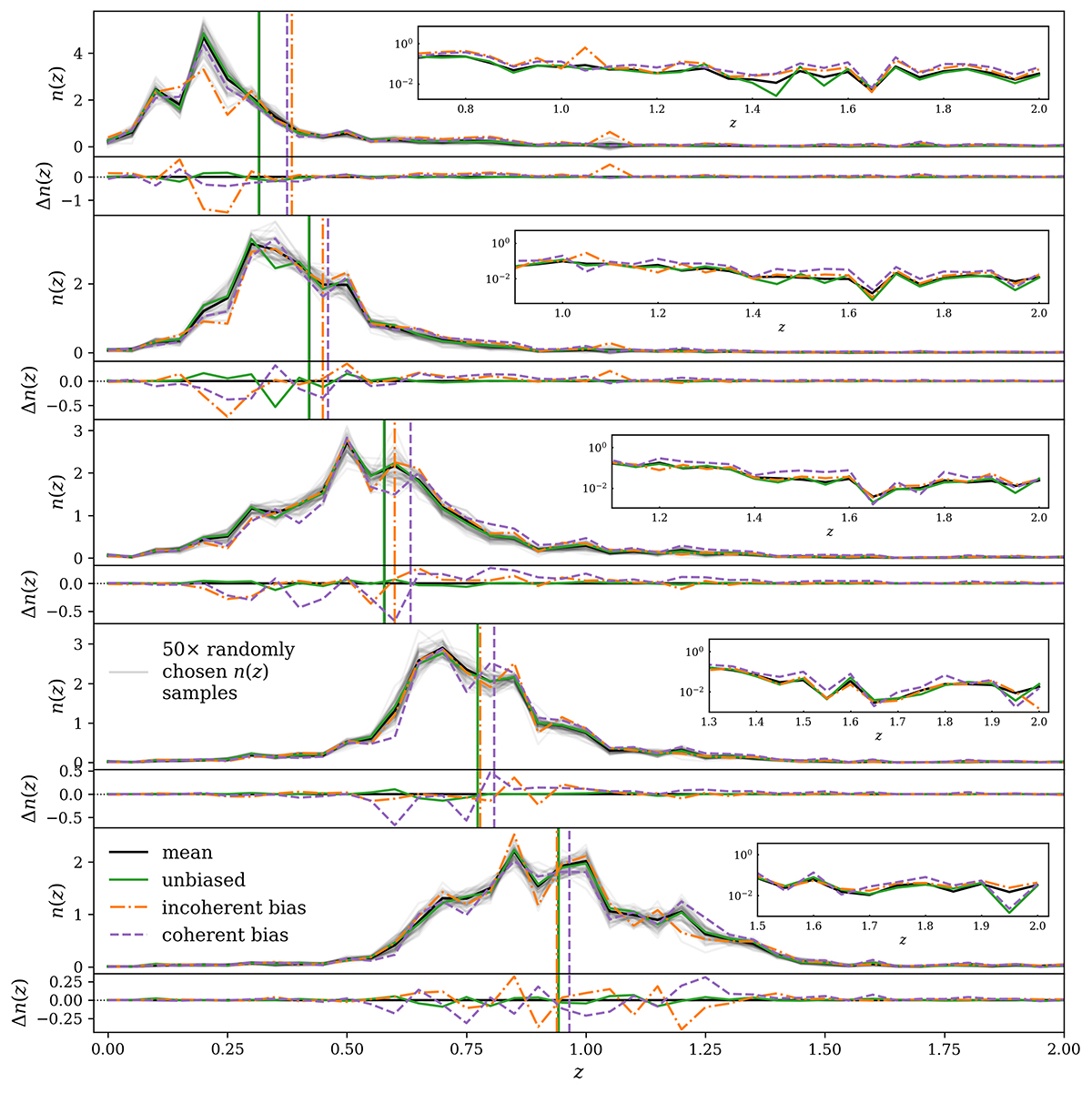
Five-bin stage III photometric redshift distributions employed in our forecasts, with alternating panels showing the distribution n_i(z) of bin i and its difference Δn_i(z) = n_i(z)−N_i(z) with respect to the ‘mean’ distribution N_i(z). Black curves in each panel correspond to the mean distribution N(z), taken as the final, public KiDS+VIKING-450 estimate (Hildebrandt et al. 2020; Wright et al. 2019). As described in Sect. 3.1.1, we assume a multivariate Gaussian distribution described by the mean N(z) and covariance Σ_n(z) (Fig. 3) to generate 45 000 sample redshift distributions, a random 50 of which are shown in n(z) panels as faint grey curves. After discarding the 80% of samples with negative n(z) values, the tomographic mean distance metrics Δ_incoherent and Δ_coherent (Eq. (3.1)) are used to select the most deviant (with respect to the mean N(z)) of the remaining samples: the ‘incoherently’ $n_z^{\mathrm{inc}}$ and ‘coherently’ $n_z^{\mathrm{coh}}$ shifted distributions, shown in each panel as dash-dotted orange and dashed purple curves, respectively. The least deviant (in terms of Δ_incoherent) sample is also selected as the ‘unbiased’ distribution, given by green curves. Inset panels zoom in on the high-z tails of each tomographic distribution, revealing small deviations there with logarithmic y-axes.