| Issue |
A&A
Volume 698, June 2025
|
|
|---|---|---|
| Article Number | A85 | |
| Number of page(s) | 17 | |
| Section | Astrophysical processes | |
| DOI | https://doi.org/10.1051/0004-6361/202553941 | |
| Published online | 03 June 2025 | |
No evidence that the binary black hole mass distribution evolves with redshift
1
Universiteit Antwerpen, Prinsstraat 13, 2000 Antwerpen, Belgium
2
Theoretische Natuurkunde, Vrije Universiteit Brussel, Pleinlaan 2, B-1050 Brussels, Belgium
3
Kavli Institute for Cosmological Physics, The University of Chicago, 5640 S. Ellis Ave., Chicago, IL 60615, USA
⋆ Corresponding author: This email address is being protected from spambots. You need JavaScript enabled to view it.
Received:
28
January
2025
Accepted:
15
April
2025
Abstract
Context. The mass distribution of merging binary black holes is generically predicted to evolve with redshift and to reflect systematic changes in their astrophysical environment, stellar progenitors, and/or dominant formation channels over cosmic time. Whether this effect is observed in gravitational-wave data remains an open question, however, and some contradictory results have been reported.
Aims. We study the ensemble of binary black holes within the latest GWTC-3 catalog released by the LIGO-Virgo-KAGRA Collaboration. We systematically searched for a possible evolution of their mass distribution with redshift.
Methods. We specifically focused on two key features in the primary mass distribution of a binary black hole: (1) an excess of 35 M⊙ black holes, and (2) a broad power-law continuum ranging from 10 to ≳80 M⊙. We determined whether one or both of these features were observed to vary with redshift.
Results. We found no evidence that either the Gaussian peak or power-law continuum components of the mass distribution change with redshift. In some cases, we placed somewhat stringent bounds on the degree of the allowed redshift evolution. Most notably, we found that the mean location of the 35 M⊙ peak and the slope of the power-law continuum are constrained to remain approximately constant below redshift z≈1. The data remain more agnostic about other forms of a dependence on redshift, such as the evolution in the height of the 35 M⊙ excess or the minimum and maximum black hole masses. We conclude that a redshift-dependent mass spectrum remains possible for all cases, but it is not required by the current data.
Key words: gravitational waves / methods: data analysis / stars: black holes
© The Authors 2025
 Open Access article, published by EDP Sciences, under the terms of the Creative Commons Attribution License (https://creativecommons.org/licenses/by/4.0), which permits unrestricted use, distribution, and reproduction in any medium, provided the original work is properly cited.
This article is published in open access under the Subscribe to Open model. This email address is being protected from spambots. You need JavaScript enabled to view it. to support open access publication.
1. Introduction
The LIGO-Virgo-KAGRA Collaboration (LVK, Aasi et al. 2015; Acernese et al. 2015; Akutsu et al. 2021) has published the detection of 90 gravitational-wave signals from merging compact binaries (Abbott et al. 2023a) to date. This growing body of gravitational-wave observations provides ever more detailed information about the properties of compact binary mergers (Abbott et al. 2023b; Callister 2024) by offering a census of their masses, spins, and the merger rate in the local Universe.
The majority of the observed gravitational waves originates from the mergers of stellar-mass binary black holes in the relatively local Universe. Gravitational-wave observations are not limited to the local Universe, however; the detection horizon of the Advanced LIGO and Virgo network now extends to or beyond redshift z≈1 (Abbott et al. 2023a; Capote et al. 2025). In addition to studying the demographics of local compact binary mergers, we therefore have an opportunity to study how these demographics systematically evolve over cosmic time. The merger rate of binary black holes, for example, is observed to increase with redshift (Abbott et al. 2023b; Callister & Farr 2024; Edelman et al. 2023), and binary black holes that merged at earlier cosmic times may have had different spin distributions than those that merge today (Biscoveanu et al. 2022; Heinzel et al. 2024).
Within this context, a commonly asked question is whether the mass distribution of merging black holes evolves with redshift. A redshift-dependent mass distribution is a generic and robust astrophysical prediction that arises from a variety of effects in a variety of different astrophysical scenarios. We describe the scenarios below.
Isolated binaries: The efficiency of massive black hole formation and merger is expected to depend sensitively on the metallicities of the progenitor stars (Belczynski et al. 2010, 2016; Chruslinska et al. 2018; Mapelli et al. 2019; Santoliquido et al. 2020; van Son et al. 2025). The overall evolving chemical enrichment of the Universe may therefore produce systematic shifts in the masses of merging black holes, with more massive black holes preferentially arising from low-metallicity stars that are prevalent at larger redshifts. In the extreme limit, Population III stars that formed at high redshifts from pristine primordial gas may even avoid pair-instability (Woosley & Heger 2021) and collapse to yield massive black holes that fall in or above the pair instability “mass gap” (Liu & Bromm 2020; Tanikawa et al. 2021) (although see Costa et al. 2023). The correlations between the masses and evolutionary delay times of the binaries formed in isolation may also impart a redshift dependence to the black hole mass spectrum. Low-mass binaries, for example, may be more prone to unstable mass transfer that leads to a common envelope, and they might merge more rapidly than high-mass binaries that evolve via stable mass transfer and cause an observed shift towards lighter black holes with higher redshift (van Son et al. 2022).
Mergers in dense clusters: Black holes that merge in globular clusters, young star clusters, and/or nuclear clusters (e.g., Portegies Zwart & McMillan 2000; Downing et al. 2010, 2011; Rodriguez et al. 2015) are also affected by metallicity-dependent stellar evolution, although they are dynamically influenced by many-body encounters. They may therefore exhibit a redshift-dependent mass distribution (Mapelli et al. 2021, 2022; Torniamenti et al. 2024). Dense clusters can also foster the assembly of massive black holes via repeated hierarchical mergers (Antonini & Rasio 2016; Fishbach et al. 2017; Antonini et al. 2019; Gerosa & Fishbach 2021; Zevin & Holz 2022; Mahapatra et al. 2025). These hierarchical mergers preferentially occur early in the lifetime of clusters, such that the masses of merging black holes are again systematically higher at high redshifts (Antonini & Rasio 2016; Ye & Fishbach 2024; Torniamenti et al. 2024).
Active galactic nuclei: Black hole mergers may instead be produced in the accretion disks of active galactic nuclei (AGN; McKernan et al. 2012; Bellovary et al. 2016; Stone et al. 2017; Ford & McKernan 2022). Merger products may themselves become trapped in the accretion disk, which leads to possibly large numbers of hierarchical mergers that build up ever more massive black holes. Massive hierarchical mergers become increasingly prevalent late in the lifetime of an AGN (Delfavero et al. 2024), possibly yielding a redshift-dependent mass distribution.
Multiple formation channels: Finally, the evolution of the black hole mass function with redshift may arise simply from the presence of multiple binary formation channels. Different formation channels generically predict distinct black hole mass distributions and naturally vary in prevalence as a function of redshift. As mixture fractions between formation channels evolve, so does the overall mass distribution (e.g., Antonini & Rasio 2016; Zevin et al. 2021; Wong et al. 2021; Mapelli et al. 2022; Torniamenti et al. 2024; Fishbach 2025).
Some authors (Farr et al. 2019; Mastrogiovanni et al. 2021) have also discussed the possibility of measuring the Hubble expansion H0 using gravitational-wave sirens, assuming a certain mass-redshift dependence of the binary black hole mass distribution, regardless of its dependence on redshift. The precise shape and redshift dependence of the mass distribution is important because it helps us to break the degeneracy between the source mass and redshift and influences the inference of cosmological parameters.
Motivated by these predictions, several studies have searched for a redshift evolution in the observed black hole mass spectrum. The results differed sometimes. Fishbach et al. (2021) searched for a redshift dependence in the maximum observed black hole mass using binary black holes from the second Gravitational-Wave Transient Catalog, GWTC-2 (Abbott et al. 2021a). On the other hand, van Son et al. (2022) investigated the relative prevalence of stable mass transfer versus common envelope evolution among isolated binaries by searching GWTC-2 data for a resulting redshift-dependent mass distribution among binary black holes (Abbott et al. 2021a). Both studies yielded null results. The study performed by Fishbach et al. (2021) was later repeated by the LVK Collaboration using additional data from GWTC-3 (Abbott et al. 2023b). No redshift dependence was reported. Ray et al. (2023) and Heinzel et al. (2025) instead employed flexible non-parametric methods that were based on the discretization of the population into a large number of piecewise constant bins, to measure the black hole mass distribution across a range of redshifts. Although this increased model flexibility translated into large uncertainties in the high-redshift mass distribution, neither study found a correlation between the black hole masses and redshifts.
On the other hand, Karathanasis et al. (2023) instead argued that current gravitational-wave data favor a large systematic shift toward higher masses between z = 0 and z = 1. They interpreted this result as a metallicity dependence in the pair-instability supernova limit for black hole masses (Heger & Woosley 2002; Farmer et al. 2019). More recently, Rinaldi et al. (2024) obtained similar conclusions by identifying an even more dramatic evolution of the black hole mass distribution with redshift, such that the most common black hole masses shifted from ∼10 solar masses in the local Universe to ∼50 M⊙ at z = 1.
Because of the difference that exists in the literature, our goal in this paper is to revisit the question of whether current gravitational-wave data indicate a redshift-dependent black hole mass distribution. Previous analyses with nonparametric models (Ray et al. 2023; Heinzel et al. 2025; Rinaldi et al. 2024) nominally minimized the systematic biases, but were in turn subject to elevated statistical uncertainties. Conversely, previous analyses performed with stronger modeling assumptions (Fishbach et al. 2021; van Son et al. 2022; Abbott et al. 2023b) greatly restricted the possible ways in which a redshift-dependence mass distribution might show itself. Rinaldi et al. (2024) hypothesized that their result was not previously observed precisely because previous analyses adopted models that were incapable of fitting their particular manner of redshift evolution.
Our goal is to bridge the gap between these approaches by measuring the redshift evolution of the black hole mass function using parametric models (to minimize the statistical uncertainty) that are nevertheless significantly more flexible than those adopted in previous work (that minimized systematic uncertainties). Gravitational-wave data confidently support the existence of two features in the black hole mass spectrum: an excess of mergers with primary masses m1≈35 M⊙, and a broad power-law continuum ranging between 10 to 80 M⊙ (Abbott et al. 2021b, 2023b; Tiwari 2022; Edelman et al. 2023; Farah et al. 2023; Callister & Farr 2024). We focus on each of the features in turn and determine whether either or both exhibit any redshift dependence in their parameters. We adopt an approach that is expected to be able to recover the redshift evolution identified by Rinaldi et al. (2024) and Karathanasis et al. (2023), if it exists. We find that current data show no evidence for a redshift-dependent binary black hole mass distribution and in some cases place informative limits on the degree of the allowed evolution. However, although no evidence for a redshift evolution is found, we note that current results do not exclude a redshift dependence either: Future analyses with expanded gravitational-wave catalogs could reveal (or further limit) evidence for a cosmically varying black hole mass distribution.
The remainder of this paper is organized as follows. In Section 2 we describe our analysis and include the precise models we used to search for and constrain a redshift-dependent mass spectrum. In Section 3 we present and discuss our resulting constraints for the redshift dependence of the mass distribution, and in Section 4, we discuss the mass-dependence of the merger rate. Finally, we conclude and discuss the astrophysical implications of this work in Section 5.
2. Methods and data
The primary mass distribution of merging binary black holes is well characterized by the superposition of a Gaussian peak near m1≈35 M⊙ and a broad power-law distribution  , with α≈−3.5. We therefore adopted the following parameterization as a baseline model for the primary mass distribution of the black hole (Talbot & Thrane 2018; Abbott et al. 2021b):
 (1)
(1)
Here, α is the slope of the power-law component and μm and σm are the mean and standard deviation, respectively, of the Gaussian component. The hyperparameter fp governs the relative height of each component, and  and ℬ are normalization constants. The goal of this work is to investigate a possible redshift dependence in Eq. (1). Concretely, we mainly focus on two questions:
-
Whether the inferred hyperparameters of the Gaussian excess (its mean, variance, and height) vary with redshift, and
-
whether the inferred hyperparameters of the power-law continuum (its boundaries, its slope, and/or the fraction of events in the continuum) vary with redshift.
These two scenarios are illustrated schematically in Figure 1, which shows a varying Gaussian peak (left) and a varying power-law continuum (right).
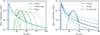 |
Fig. 1. Cartoon illustrating the possible manners, as considered in this work, in which the primary mass distribution of a binary black hole might evolve with redshift. As illustrated in the left panel, we consider the possibilities that the location, width, and/or height of the 35 M⊙ excess evolve with redshift (see Sect. 3.1). As illustrated on the right, we allowed for the evolution of the height, slope, and endpoints of the power-law continuum (see Sect. 3.2). |
2.1. Modeling a redshift-dependent mass distribution
In order to answer the above questions, we promoted the hyperparameters in Eq. (1) to functions of redshift. In particular, we allowed the hyperparameters of interest to vary as sigmoids. This enabled a flexible and smooth transition between low- and high-redshift values. In particular, when Λ signifies an arbitrary hyperparameter (e.g. α and μm), then we assumed that Λ evolves as
![Mathematical equation: $$ \Lambda (z) = \frac {\Lambda _{\mathrm {high}} - \Lambda _{\mathrm {low}}}{1 + \exp \left [-\frac {1}{\Delta z_\Lambda }\left (z - \bar z_\Lambda \right ) \right ]} + \Lambda _{\textrm {low}}. $$](/articles/aa/full_html/2025/06/aa53941-25/aa53941-25-eq4.gif) (2)
(2)
where Λlow is the hyperparameter value at redshift  and Λhigh is the value that is asymptotically approached at
  . The transition occurs across a redshift interval with a width ΔzΛ centered at
  .
.
2.2. Defining the differential merger rate
Together with the (redshift-dependent) primary mass distribution, we simultaneously measured the secondary mass distribution of the binary black hole, the spin distribution, and the overall evolution of the merger rate with redshift. Our full model for the source-frame merger rate of binary black holes took the form
 (3)
(3)
The above quantity denotes the number of mergers per unit of comoving volume dVc, per unit source frame time dts, and per unit source parameters. The function ϕ(m1|z) encodes the primary mass distribution at a given redshift. This is given by Eq. (1), with additional smoothing factors that truncate the mass distribution at sufficiently low and high values Mmin and Mmax,
 (4)
(4)
Here, p(m1|z) is as given Eq. (1), but the hyperparameters are promoted to functions of redshift, as described in Section 2.1. Similarly, the hyperparameters that control the truncation of the mass distribution, such as Mmin and Mmax and the widths of the smoothing exponentials δmmin and δmmax, were also regarded as functions of redshift using the aforementioned sigmoid formalism.
Within Eq. (3), the function f(z) captures the overall (mass-independent) evolution of the merger rate with redshift. If merging black holes are of stellar origin, then the merger rate is likely to qualitatively trace cosmic star formation, which initially rises as a function of redshift before it peaks and decreases at higher redshift (Madau & Dickinson 2014; Madau & Fragos 2017). Accordingly, we adopted a model (Fishbach et al. 2018; Callister et al. 2020),
 (5)
(5)
which grows as f(z)∝(1+z)αz at z≪zp and decreases as f(z)∝(1+z)−βz at z≫zp.
We also assumed a power-law distribution for the secondary mass of the binary, such that (Fishbach & Holz 2020)
 (6)
(6)
In principle, we might additionally have included the power-law slope βq among the parameters we allowed to vary with redshift, when doing so, however, only uninformative constraints, and so for simplicity exclude variation in βq in the analyses discussed in Section 3. Our models for the probability distributions of the component spins χ1 and χ2 are described in Appendix A. The overall normalization of the merger rate is captured in Eq. (3) by Rref, which is the differential merger rate evaluated at z = 0.2 and m1 = 20 M⊙. These reference points correspond to locations at which the differential merger rate is reasonably well measured, which improves the sampling efficiency when the model hyperparameters are inferred. Beyond algorithmic efficiency, however, the choice of the reference point does not affect our results. Different reference points would simply alter the posterior on Rref by a multiplicative constant.
2.3. Data and likelihood
We considered all binary black hole events in the LIGO-Virgo-KAGRA Collaboration GWTC-3 catalog (Abbott et al. 2023a) with false alarm rates below one per year. When a binary black hole population is described by hyperparameters Λ, the likelihood of an observed gravitational-wave catalog is (Loredo 2004; Taylor & Gerosa 2018; Mandel et al. 2019; Vitale et al. 2020)
 (7)
(7)
Here, Nobs is the total number of gravitational-wave observations, with the data represented by  , and Nexp(Λ) is the total number of expected mergers (observed or unobserved) that are predicted to occur over the given observation period. In the above likelihood, λ signifies the individual parameters (component masses, spins, redshift, etc.) of each binary; the likelihood of the i’th gravitational-wave event given parameters λ is denoted p(di|λ). The quantity dN/dλ(Λ) is the detector-frame rate of gravitational-wave events, which is related to the source-frame rate in Eq. (3) by
 (8)
(8)
where the factor (1+z)−1 transforms from detector-frame into source-frame time, Tobs is the observing time, and dVc/dz gives the comoving volume per unit redshift.
In practice, we evaluated Eq. (7) not as an integral over the event likelihoods, but instead via Monte Carlo averages over discrete posterior samples for each event. For the sets of samples {λ}∼p(λ|di) drawn from each event posterior, Eq. (7) may be approximated via
 (9)
(9)
where ppe(λi) is the prior used during parameter estimation and 〈·〉samples indicates an average taken over posterior samples of a given event.
The search selection effects are captured by the expected number of detections, Nexp(Λ), given by
 (10)
(10)
where Pdet(λ) is the probability of detecting an event with event parameters λ. This integral, can also be approximated as a Monte Carlo average over simulated signals injected into and recovered from gravitational-wave data. Given a total number Ninj of such injections, each drawn from a parent distribution pinj(λ),
 (11)
(11)
where the summation runs over the subset of successfully recovered injections. More information about the exact data we used in our analysis can be found in Appendix B.
3. Evolution of the black hole mass spectrum with redshift
As discussed previously, the primary mass distribution of the binary black hole can be phenomenologically modeled as two pieces: (i) a Gaussian excess situated on top of (ii) a broad power-law continuum. We searched for the redshift evolution within each of these features in turn. In Section 3.1 we first explore the degree to which the Gaussian peak evolves with redshift. In Section 3.2 we then examine a possible redshift evolution in the power-law continuum1. In Section 4 we reverse our perspective and instead analyze GWTC-3 data in search of a mass dependence in the redshift distribution of binary black holes.
3.1. Variation in the Gaussian excess with redshift
The Gaussian excess observed in the primary mass distribution of a binary black hole is governed by three parameters: the mean of the peak μm, its standard deviation σm, and the mixing fraction fp that controls its relative height. We varied each of these hyperparameters as a function of redshift, as in Eq. (2), using the priors described in Appendix A.
Figure 2 shows our resulting constraints on the redshift-dependent mass distribution when the Gaussian peak was allowed to evolve. In particular, we show the probability distribution of primary masses taken at two different redshifts: z = 0.2 (upper panel) and z = 0.75 (lower panel).
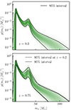 |
Fig. 2. Inferred primary mass distribution of a binary black hole, when the Gaussian excess at ∼35 M⊙ evolves with redshift. Upper panel: Inferred primary mass distribution at z = 0.2. Green traces illustrate individual draws from our hyperposterior, and the solid black lines mark the 95% credible bounds. Lower panel: Primary mass distribution inferred at z = 0.75. For comparison, the dashed black lines illustrate the 95% credible bounds from the upper panel at z = 0.2. |
Fig. 2 shows that the location of the peak is constrained to remain reasonably stationary across the full range of redshifts we considered. Specifically, μm can shift by no more than 17% between z = 0 and z = 1, at a credibility of 90%. At the same time, the height of the peak is less well constrained; a more pronounced and growing 35 M⊙ peak at higher redshift is not excluded by the current observations. This growth is not required, but it indicates that current gravitational-wave catalogs contain no affirmative evidence for a redshift-dependent peak.
An alternative view of our results is given in Fig. 3, which shows our posteriors on the relevant hyperparameters themselves as a function of redshift. Specifically, the top, middle, and lower panels show our posteriors on the location μm(z), width σm(z), and logarithmic height of the peak log fp(z).
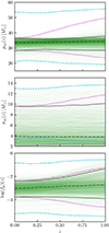 |
Fig. 3. Inferred values of the hyperparameters characterizing the mean (top), standard deviation (middle), and height (bottom) of the Gaussian peak in the black hole mass spectrum as a function of redshift. In each panel, the green traces mark individual hyperposterior samples, and the solid and dot-dashed black curves indicate 95% credible posterior bounds and medians, respectively. The dashed cyan lines analogously illustrate 95% credible prior bounds. Finally, the dotted magenta curves indicate 95% credible prior bounds on each parameter when it is first conditioned on the measured posteriors at z = 0. |
In all three cases (and for μm(z) and log fp(z) in particular), our posteriors are constrained away from our priors in a broad range of redshifts. At face value, however, the interpretation of these measurements is ambiguous: It is unclear whether we meaningfully measured these parameters across a range of redshifts or if we only succeeded in measuring them at z≈0, with the high-redshift posteriors constituting simply a prior-dependent extrapolation of these low-redshift bounds.
To answer this question, we show the conditional priors on each parameter as dotted magenta curves, given our posteriors at z = 0. These curves illustrate the remaining redshift dependence allowed by our prior, when it is informed by data at z = 0 alone, and the curves accordingly demonstrate the degree to which low-redshift information is or is not being extrapolated to high redshifts.
By comparing our posterior on μm(z) to this conditional prior, we see that the posterior is constrained well away from the conditional prior at high redshifts. The conclusion that μm(z) must remain relatively constant therefore is a feature of the data and not an artifact of our prior. Our posterior on σm(z), on the other hand, is marginally constrained away from the conditional prior, but it is apparent that additional data are required before we can obtain informative constraints on the width of the 35 M⊙ peak with redshift. Our lower bound on log fp(z) is in turn strongly constrained away from the conditional prior, such that we can confidently conclude that the 35 M⊙ peak does not shrink with redshift. In contrast, the upper bound on log fp(z) coincides with the conditional prior, such that any apparent growth in the 35 M⊙ peak (e.g. the lower panel of Fig. 2) purely is a prior effect. As shown by the conditional priors, the results at z≥0.5 are not just extrapolations from z = 0, but the results at z≈1 are probably extrapolations from an intermediate redshift. A corner plot showing the full posterior on the hyperparameters governing μm(z) is given in Appendix C.
3.2. Evolution of the power-law continuum with redshift
Next, we instead studied whether the observed binary black holes exhibited evidence for a redshift-dependent power-law continuum. This continuum is defined by a set of six parameters: a power-law index α, the truncation points Mmin and Mmax, the mass scales δmmin and δmmax over which the truncation occurs, and the relative height of the continuum given by 1−fp.
Figure 4 shows the resulting constraints on the black hole primary mass distribution at z = 0.2 (upper panel) and z = 0.75 (lower panel). As in Fig. 2, the figure shows no systematic evidence that the black hole mass distribution evolves with redshift. The only noticeable difference in p(m1) between the high and low redshifts is the possible change in the height of the power-law continuum (which is compensated for by an equal and opposite change in the height of the Gaussian peak). We cannot rule out a redshift variation on scales finer than we can currently probe with the existing data.
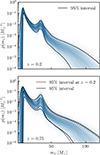 |
Fig. 4. As in Fig. 2, but the power-law continuum of the binary black hole primary mass spectrum evolves with redshift. |
In Fig. 5 we plot posteriors on relevant hyperparameters as a function of redshift. We specifically show redshift-dependent constraints on the continuum power-law index α(z), the log mixing fraction, log fp(z), and the minimum mass Mmin(z) below which the primary mass distribution is truncated. Our posteriors on other parameters, such as the maximum black hole mass Mmax and truncation scale lengths, do not deviate from their corresponding conditional priors and are therefore not shown.
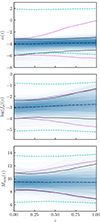 |
Fig. 5. As in Fig. 3, but showing posteriors on the redshift-dependent hyperparameters that characterize the power-law continuum. Specifically, we show posteriors on the power-law slope (top), mixing fraction (middle), and the location below which the mass distribution is truncated (bottom). The posteriors on other parameters (e.g. the maximum black hole mass and high- or low-mass truncation scales) are uninformative and are not shown here. |
The power-law index α(z) is well measured across a range of redshifts that is bounded confidently away (both above and below) from the conditional prior. At the same time, there is no evidence for a systematic shift in this slope. Interestingly, the power-law index appears to be marginally better constrained at higher redshifts than at low redshift. We attribute this to the fact that the power-law slope is strongly informed by high-mass mergers. Because these are rare, they are primarily seen at higher redshifts. The fact that these events are observed sets a lower bound on α(z) at high z, as a sufficiently negative α(z) would predict too few observable events. In contrast, very few high-mass mergers have been identified at low redshift. This can be explained simply by their overall rarity combined with a nonevolving mass distribution, but it can also be explained by a more negative α(z) acting in the local Universe. Altogether, we find that α is permitted to vary by up to 31% between redshifts z = 0 and 1 at 90% credibility.
The posterior on the mixing fraction fp(z) is quite similar in behavior to that shown in Fig. 3. It is bounded above the conditional prior given by the measured continuum and peak heights at z = 0. It therefore remains possible that the height of the power-law continuum decreases with redshift (offset by an increase in the height of the Gaussian peak), but the data show no affirmative evidence of this behavior. Finally, there is very little information regarding the evolution of Mmin with redshift. Its posterior shifts very little relative to the conditional prior on Mmin(z), but it remains possible for Mmin to both rise or fall with redshift. Corner plots showing the full posterior hyperparameters that control log fp(z) and α(z) are given in Appendix C.
4. Variation in the black hole redshift distribution with mass
In Section 3 we explored the constraints on the systematic evolution of the primary mass distribution of the binary black hole with redshift, but we found no evidence for any evolution. This is not the only way to frame this observational question, however. The merger rate of binary black holes is known to rise as a function of redshift. Therefore, instead of asking whether the black hole mass distribution depends on redshift, this question can be inverted to ask whether the increase rate in the merger rate depends on the mass.
These two questions are not independent of each other. However, different astrophysical scenarios may be better modeled by one approach than by the other (a redshift-dependent mass distribution versus a mass-dependent redshift distribution). Different binary formation channels (e.g. stellar clusters, a common envelope, or stable mass transfer) are generically expected to trace different redshift-dependent merger histories. If the observed binary black hole population is itself composed of systems from several such channels, each of which dominates in a different mass regime, then the resulting redshift-dependent merger rate may naturally be well modeled by Eq. (5) but with hyperparameters that vary as a function of mass.
To explore this possibility, we followed the same method as in Section 2 but inverted the roles of mass and redshift. Specifically, we elevated the parameters αz, βz, and zp that characterize the redshift-dependent merger rate (see Eq. (5)) to be functions of primary mass: αz(m1), βz(m1), and zp(m1). Each of these were modeled as sigmoids,
![Mathematical equation: $$ \Lambda (m_1) = \frac {\Lambda _{\mathrm {high}} - \Lambda _{\mathrm {low}}}{1 + \exp \left [-\frac {1}{\Delta m_\Lambda }\left (m_1 - \bar m_\Lambda \right ) \right ]} + \Lambda _{\textrm {low}}. $$](/articles/aa/full_html/2025/06/aa53941-25/aa53941-25-eq18.gif) (12)
(12)
Analogous to Eq. (2), Λ stands for one of the hyperparameters {αz, βz, zp}, with Λ(m1) transitioning from Λlow at masses  to Λhigh at
  across an interval of scale width ΔmΛ. Our full model for the redshift-dependent merger rate becomes
 (13)
(13)
(compare to Eq. (3)).
In Fig. 6 we show the resulting posteriors on the low-redshift power-law slope αz(m1) and the peak redshift zp(m1) as a function of m1. The data are entirely uninformative regarding the high-redshift slope βz(m1) and we therefore do not show a posterior on this parameter. Our posterior on αz(m1) in the upper panel shows very marked behavior. At low primary masses αz(m1) is broadly constrained to lie between −4.1≤αz≤4.3 at 95% credibility. The posterior then undergoes a rapid transition around 35 M⊙, such that αz(m1 = 35 M⊙) is bounded between 0.7 and 5.1 at 95% credibility. The posterior subsequently slightly broadens again at higher masses. This behavior is expected. By virtue of search-selection functions, a large number of binaries with m1≈35 M⊙ are observed out to large distances, which provides a reasonably precise measurement of αz in this mass range. In contrast, only a few low-mass binaries are observed, and those that are detected lie at low redshifts. We therefore currently have little information about αz for low-mass events. The nonzero number of detected massive binaries at large redshifts also yields a lower limit on αz for high-mass events, although with somewhat broader uncertainties that are set by the relatively small number of these events.
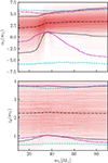 |
Fig. 6. Constraints on the power-law slope αz that governs the evolution of the volumetric binary black hole merger rate with redshift (top) and the peak redshift zp beyond which the merger rate turns over (bottom), each as as function of primary mass. As in Figs. 3 and 5, the black lines show the 95% credible posterior bounds, the dashed cyan lines mark prior bounds, and the dotted magenta curves illustrate prior bounds after they were conditioned on the best-measured posteriors at m1 = 35 M⊙. |
Analogously to Figs. 3 and 5, the dotted magenta curves show conditional priors on αz(m1). In these previous figures, we showed priors conditioned on measurements at z = 0, at which redshift we obtained the most precise measurement of the black hole mass distribution. In this context, it is clear that the black hole redshift distribution is most precisely measured at m1≈35 M⊙. We accordingly conditioned priors at this location, which resulted in the waist that appears in the upper panel of Fig. 6. The deviation between our αz(m1) posterior and the conditional prior indicates additional information in the data. At high masses, the data disfavor low or negative values of αz. At low masses, although the posterior and conditioned prior largely coincide, the posterior is nevertheless pushed to slightly smaller values of αz. This might indicate a distinct redshift evolution of low- and high-mass binary black holes.
The lower panel of Fig. 6 similarly shows our prior, posterior, and conditional prior on zp(m1). The peak redshift is bounded away from zero in the 30–50 M⊙ range because very many events are observed in this mass range. Otherwise, the posterior is largely uninformative and closely followes the conditional prior at lower and higher masses.
Despite the nontrivial constraints on αz(m1), we found no requirement on the whole that the black hole redshift distribution varies as a function of mass. The current data remain consistent with a population whose merger rate evolves synchronously across the full mass range, with single, universal values of αz and zp. Additional results are discussed in Appendix C, including corner plots that illustrate full posteriors on the hyperparameters governing αz(m1) and zp(m1).
5. Conclusion
We have systematically surveyed current gravitational-wave data for a redshift-dependence in the mass spectrum of binary black holes. We found no evidence for a correlation between the black hole masses and redshifts, and the present-day data are consistent with a primary mass spectrum that remains stationary with redshift.
In some cases, we identified nontrivial constraints on the degree of the redshift evolution allowed by current data. We found in Sect. 3.1 that the location of the 35 M⊙ peak in the black hole primary mass spectrum remains relatively fixed across a broad range of redshifts; its mean can shift by only 17% or less between z = 0 to z = 1. Similarly, we found in Sect. 3.2 that the slope of the power-law continuum is approximately constant out to redshift z≈1. It varies by less than 31% from z = 0 to z≈1. These constraints may already be sufficient to rule out theoretical models that predict a large-scale evolution of black hole masses with redshift. At the same time, systematic variation in the black hole masses with redshift is not excluded. For example, the current data are still consistent with scenarios in which the height of the 35 M⊙ peak rises or falls somewhat considerably with redshift (see Sect. 3). We emphasize, however, that this evolution is not a requirement of the data.
These results differ from the conclusions drawn by Karathanasis et al. (2023) and Rinaldi et al. (2024), but are consistent with results of other analyses (Fishbach et al. 2021; van Son et al. 2022; Abbott et al. 2021a; Ray et al. 2023; Heinzel et al. 2025). The ultimate source of this disagreement is unclear to us. In preparing our results, we found that spurious redshift evolution might be introduced if we did not check for and control the poor convergence in the Monte Carlo integrals [e.g. Eqs. (9) and (11)] that appear in the population likelihood (Farr 2019; Essick & Farr 2022; Talbot & Golomb 2023). It is possible that similar issues might have been responsible for previous claims of mass-redshift correlations. While our work reached its final stages of preparation, we were additionally made aware of a complementary study that applied the method of Sadiq et al. (2024) to explore the redshift variation in the black hole masses (Sadiq et al. 2025). This study reported no statistically significant evidence for an evolving mass distribution with GWTC-3. This is consistent with our results.
We note that, although we adopted a more flexible model than previous parametric analyses, we nevertheless assumed that the black hole mass distribution is well described by the mixture of a power law and a Gaussian. This necessarily introduces some degree of systematic uncertainty. Although this model matches the most confident features in the black hole mass distribution, there are also signs that the mass distribution is somewhat more complex, with a narrower global maximum near 10 M⊙ and a possible steepening at very high masses. It is possible that the redshift dependence in these additional features might be missed in our current analysis. Future work might correspondingly adopt a more complex model to target these features.
Although the current data do not yet indicate a correlation between black hole redshifts and mass (subject to the above caveat), it would be surprising if no correlation were fundamentally present because these correlations may arise in very many different ways (see Sect. 1). Instrumental upgrades and continued commissioning leading up to and during the current LIGO-Virgo-KAGRA O4 observing run increase the distance to which binary black holes can be detected and the precision with which they can be characterized (Capote et al. 2025), and we anticipate that future catalogs may yet reveal a black hole mass spectrum that changes over cosmic time. If a mass-redshift correlation remains unobserved, however, the astrophysical implications of a null result become increasingly important. A mass distribution that is known to remain constant over a wide range of redshifts may indicate that binary black holes experience very long time delays between their formation and eventual merger. This would wash out the time varying conditions present at their birth. This might indicate that the formation of massive black holes is much less dependent on stellar metallicity than typically expected (e.g., van Son et al. 2025), and/or that metal-poor environments remain prevalent even at late cosmic times. Finally, it would likely indicate that no more than one formation channel contributes non-negligibly to the observed population of black hole mergers.
Data availability
Code used to perform this study is made available on GitHub at [https://github.com/maxlalleman/bbh_mass_distribution_redshift_variation_inference], and datasets comprising our results are available on Zenodo at https://zenodo.org/records/14671139.
Acknowledgments
K. T. was supported by FWO-Vlaanderen through grant number 1179524N. T. C. is supported by the Eric and Wendy Schmidt AI in Science Postdoctoral Fellowship, a Schmidt Sciences program. This research has made use of data, software and/or web tools obtained from the Gravitational Wave Open Science Center (https://www.gw-openscience.org), a service of LIGO Laboratory, the LIGO Scientific Collaboration and the Virgo Collaboration. Virgo is funded by the French Centre National de Recherche Scientifique (CNRS), the Italian Istituto Nazionale della Fisica Nucleare (INFN) and the Dutch Nikhef, with contributions by Polish and Hungarian institutes. This material is based upon work supported by NSF's LIGO Laboratory which is a major facility fully funded by the National Science Foundation. The authors are grateful for computational resources provided by the LIGO Laboratory and supported by NSF Grants PHY-0757058 and PHY-0823459. Software: arviz (Kumar et al. 2019), astropy (Astropy Collaboration 2013, 2018), jax (Bradbury et al. 2018), matplotlib (Hunter 2007), numpy (Harris et al. 2020), numpyro (Phan et al. 2019; Bingham et al. 2019), scipy (Virtanen et al. 2020).
References
- Aasi, J., Abbott, B. P., Abbott, R., et al. 2015, Class. Quantum Grav., 32, 074001 [CrossRef] [Google Scholar]
- Abbott, B. P., Abbott, R., Abbott, T. D., et al. 2019, Phys. Rev. X, 9, 031040 [Google Scholar]
- Abbott, R., Abbott, T. D., Abraham, S., et al. 2020, ApJ, 896, L44 [Google Scholar]
- Abbott, R., Abbott, T. D., Abraham, S., et al. 2021a, Phys. Rev. X, 11, 021053 [Google Scholar]
- Abbott, R., Abbott, T. D., Abraham, S., et al. 2021b, ApJ, 913, L7 [NASA ADS] [CrossRef] [Google Scholar]
- Abbott, R., Abbott, T. D., Abraham, S., et al. 2021c, SoftwareX, 13, 100658 [NASA ADS] [CrossRef] [Google Scholar]
- Abbott, R., Abbott, T. D., Acernese, F., et al. 2023a, Phys. Rev. X, 13, 041039 [Google Scholar]
- Abbott, R., Abbott, T. D., Acernese, F., et al. 2023b, Phys. Rev. X, 13, 011048 [NASA ADS] [Google Scholar]
- Abbott, R., Abe, H., Acernese, F., et al. 2023c, ApJS, 267, 29 [CrossRef] [Google Scholar]
- Acernese, F., Agathos, M., Agatsuma, K., et al. 2015, Class. Quantum Grav., 32, 024001 [CrossRef] [Google Scholar]
- Akutsu, T., Ando, M., Arai, K., et al. 2021, PTEP, 2021, 05A101 [Google Scholar]
- Antonini, F., & Rasio, F. A. 2016, ApJ, 831, 187 [Google Scholar]
- Antonini, F., Gieles, M., & Gualandris, A. 2019, MNRAS, 486, 5008 [NASA ADS] [CrossRef] [Google Scholar]
- Astropy Collaboration (Robitaille, T. P., et al.) 2013, A&A, 558, A33 [NASA ADS] [CrossRef] [EDP Sciences] [Google Scholar]
- Astropy Collaboration (Price-Whelan, A. M., et al.) 2018, AJ, 156, 123 [Google Scholar]
- Belczynski, K., Dominik, M., Bulik, T., et al. 2010, ApJ, 715, L138 [Google Scholar]
- Belczynski, K., Holz, D. E., Bulik, T., & O’Shaughnessy, R. 2016, Nature, 534, 512 [NASA ADS] [CrossRef] [Google Scholar]
- Bellovary, J. M., Mac Low, M. -M., McKernan, B., & Ford, K. E. S. 2016, ApJ, 819, L17 [NASA ADS] [CrossRef] [Google Scholar]
- Bingham, E., Chen, J. P., Jankowiak, M., et al. 2019, J. Mach. Learn. Res., 20, 28:1 [Google Scholar]
- Biscoveanu, S., Callister, T. A., Haster, C. -J., et al. 2022, ApJ, 932, L19 [NASA ADS] [CrossRef] [Google Scholar]
- Bradbury, J., Frostig, R., Hawkins, P., et al. 2018, JAX: Composable Transformations of Python+NumPy Programs, http://github.com/google/jax [Google Scholar]
- Callister, T. A. 2024, arXiv e-prints [arXiv:2410.19145] [Google Scholar]
- Callister, T. A., & Farr, W. M. 2024, Phys. Rev. X, 14, 021005 [NASA ADS] [Google Scholar]
- Callister, T., Fishbach, M., Holz, D. E., & Farr, W. M. 2020, ApJ, 896, L32 [NASA ADS] [CrossRef] [Google Scholar]
- Capote, E., Jia, W., Aritomi, N., et al. 2025, Phys. Rev. D, 111, 062002 [Google Scholar]
- Chruslinska, M., Nelemans, G., & Belczynski, K. 2018, MNRAS, 482, 5012 [Google Scholar]
- Costa, G., Mapelli, M., Iorio, G., et al. 2023, MNRAS, 525, 2891 [NASA ADS] [CrossRef] [Google Scholar]
- Delfavero, V., Ford, K. E. S., McKernan, B., et al. 2024, ApJ, submitting [arXiv:2410.18815] [Google Scholar]
- Downing, J. M. B., Benacquista, M. J., Giersz, M., & Spurzem, R. 2010, MNRAS, 407, 1946 [NASA ADS] [CrossRef] [Google Scholar]
- Downing, J. M. B., Benacquista, M. J., Giersz, M., & Spurzem, R. 2011, MNRAS, 416, 133 [Google Scholar]
- Edelman, B., Farr, B., & Doctor, Z. 2023, ApJ, 946, 16 [NASA ADS] [CrossRef] [Google Scholar]
- Essick, R., & Farr, W. 2022, arXiv e-prints [arXiv:2204.00461] [Google Scholar]
- Farah, A. M., Edelman, B., Zevin, M., et al. 2023, ApJ, 955, 107 [NASA ADS] [CrossRef] [Google Scholar]
- Farmer, R., Renzo, M., De Mink, S. E., Marchant, P., & Justham, S. 2019, ApJ, 887, 53 [Google Scholar]
- Farr, W. M. 2019, RNAAS, 3, 66 [Google Scholar]
- Farr, W. M., Fishbach, M., Ye, J., & Holz, D. E. 2019, ApJ, 883, L42 [NASA ADS] [CrossRef] [Google Scholar]
- Fishbach, M. 2025, Class. Quantum Grav., 42, 055009 [Google Scholar]
- Fishbach, M., & Holz, D. E. 2020, ApJ, 891, L27 [NASA ADS] [CrossRef] [Google Scholar]
- Fishbach, M., Holz, D. E., & Farr, B. 2017, ApJ, 840, L24 [NASA ADS] [CrossRef] [Google Scholar]
- Fishbach, M., Holz, D. E., & Farr, W. M. 2018, ApJ, 863, L41 [NASA ADS] [CrossRef] [Google Scholar]
- Fishbach, M., Doctor, Z., Callister, T., et al. 2021, ApJ, 912, 98 [NASA ADS] [CrossRef] [Google Scholar]
- Ford, K. E. S., & McKernan, B. 2022, MNRAS, 517, 5827 [NASA ADS] [CrossRef] [Google Scholar]
- Gerosa, D., & Fishbach, M. 2021, Nat. Astron., 5, 749 [NASA ADS] [CrossRef] [Google Scholar]
- Harris, C. R., Millman, K. J., van der Walt, S. J., et al. 2020, Nature, 585, 357 [NASA ADS] [CrossRef] [Google Scholar]
- Heger, A., & Woosley, S. E. 2002, ApJ, 567, 532 [Google Scholar]
- Heinzel, J., Biscoveanu, S., & Vitale, S. 2024, Phys. Rev. D, 109, 103006 [Google Scholar]
- Heinzel, J., Mould, M., & Vitale, S. 2025, Phys. Rev. D, 111, L061305 [Google Scholar]
- Hunter, J. D. 2007, CiSE, 9, 90 [Google Scholar]
- Karathanasis, C., Mukherjee, S., & Mastrogiovanni, S. 2023, MNRAS, 523, 4539 [NASA ADS] [Google Scholar]
- Kumar, R., Carroll, C., Hartikainen, A., & Martin, O. 2019, JOSS, 4, 1143 [Google Scholar]
- Liu, B., & Bromm, V. 2020, MNRAS, 495, 2475 [NASA ADS] [CrossRef] [Google Scholar]
- Loredo, T. J. 2004, AIP Conf. Proc., 735, 195 [CrossRef] [Google Scholar]
- Madau, P., & Dickinson, M. 2014, ARAA, 52, 415 [Google Scholar]
- Madau, P., & Fragos, T. 2017, ApJ, 840, 39 [Google Scholar]
- Mahapatra, P., Chattopadhyay, D., Gupta, A., et al. 2025, Phys. Rev. D, 111, 023013 [Google Scholar]
- Mandel, I., Farr, W. M., & Gair, J. R. 2019, MNRAS, 486, 1086 [Google Scholar]
- Mapelli, M., Giacobbo, N., Santoliquido, F., & Artale, M. C. 2019, MNRAS, 487, 2 [NASA ADS] [CrossRef] [Google Scholar]
- Mapelli, M., Dall’Amico, M., Bouffanais, Y., et al. 2021, MNRAS, 505, 339 [CrossRef] [Google Scholar]
- Mapelli, M., Bouffanais, Y., Santoliquido, F., Arca Sedda, M., & Artale, M. C. 2022, MNRAS, 511, 5797 [NASA ADS] [CrossRef] [Google Scholar]
- Mastrogiovanni, S., Leyde, K., Karathanasis, C., et al. 2021, Phys. Rev. D, 104, 062009 [NASA ADS] [CrossRef] [Google Scholar]
- McKernan, B., Ford, K. E. S., Lyra, W., & Perets, H. B. 2012, MNRAS, 425, 460 [NASA ADS] [CrossRef] [Google Scholar]
- Phan, D., Pradhan, N., & Jankowiak, M. 2019, arXiv e-prints [arXiv:1912.11554] [Google Scholar]
- Portegies Zwart, S. F., & McMillan, S. L. W. 2000, ApJ, 528, L17 [Google Scholar]
- Ray, A., Hernandez, I. M., Mohite, S., Creighton, J., & Kapadia, S. 2023, ApJ, 957, 37 [NASA ADS] [CrossRef] [Google Scholar]
- Rinaldi, S., Del Pozzo, W., Mapelli, M., Lorenzo-Medina, A., & Dent, T. 2024, A&A, 684, A204 [NASA ADS] [CrossRef] [EDP Sciences] [Google Scholar]
- Rodriguez, C. L., Morscher, M., Pattabiraman, B., et al. 2015, Phys. Rev. Lett., 115, 051101 [Google Scholar]
- Sadiq, J., Dent, T., & Gieles, M. 2024, ApJ, 960, 65 [NASA ADS] [CrossRef] [Google Scholar]
- Sadiq, J., Dent, T., & Medina, A. L. 2025, arXiv e-prints [arXiv:2502.06451] [Google Scholar]
- Santoliquido, F., Mapelli, M., Bouffanais, Y., et al. 2020, ApJ, 898, 152 [Google Scholar]
- Stone, N. C., Metzger, B. D., & Haiman, Z. 2017, MNRAS, 464, 946 [Google Scholar]
- Talbot, C., & Golomb, J. 2023, MNRAS, 526, 3495 [NASA ADS] [CrossRef] [Google Scholar]
- Talbot, C., & Thrane, E. 2018, ApJ, 856, 173 [NASA ADS] [CrossRef] [Google Scholar]
- Tanikawa, A., Susa, H., Yoshida, T., Trani, A. A., & Kinugawa, T. 2021, ApJ, 910, 30 [NASA ADS] [CrossRef] [Google Scholar]
- Taylor, S. R., & Gerosa, D. 2018, Phys. Rev. D, 98, 083017 [NASA ADS] [CrossRef] [Google Scholar]
- Tiwari, V. 2022, ApJ, 928, 155 [NASA ADS] [CrossRef] [Google Scholar]
- Torniamenti, S., Mapelli, M., Périgois, C., et al. 2024, A&A, 688, A148 [NASA ADS] [CrossRef] [EDP Sciences] [Google Scholar]
- Vallisneri, M., Kanner, J., Williams, R., Weinstein, A., & Stephens, B. 2015, J. Phys. Conf. Ser., 610, 012021 [Google Scholar]
- van Son, L. A. C., de Mink, S. E., Callister, T., et al. 2022, ApJ, 931, 17 [NASA ADS] [CrossRef] [Google Scholar]
- van Son, L. A. C., Roy, S. K., Mandel, I., et al. 2025, ApJ, 979, 209 [Google Scholar]
- Virtanen, P., Gommers, R., Oliphant, T. E., et al. 2020, Nat. Methods, 17, 261 [Google Scholar]
- Vitale, S., Gerosa, D., Farr, W. M., & Taylor, S. R. 2020, Handbook of Gravitational Wave Astronomy (Singapore: Springer) [Google Scholar]
- Wong, K. W. K., Breivik, K., Kremer, K., & Callister, T. 2021, Phys. Rev. D, 103, 083021 [Google Scholar]
- Woosley, S. E., & Heger, A. 2021, ApJ, 912, L31 [NASA ADS] [CrossRef] [Google Scholar]
- Ye, C. S., & Fishbach, M. 2024, ApJ, 967, 62 [Google Scholar]
- Zevin, M., & Holz, D. E. 2022, ApJ, 935, L20 [CrossRef] [Google Scholar]
- Zevin, M., Bavera, S. S., Berry, C. P. L., et al. 2021, ApJ, 910, 152 [Google Scholar]
Appendix A: Spin Models and Prior Information
In this appendix we provide more details regarding our spin models (not discussed in the main text) and the priors adopted on our hyperparameters during our population inference.
We assume that dimensionless component spin magnitudes are independently and identically modeled as truncated Gaussians:
 (A.1)
(A.1)
with mean μχ and variance  . Similarly, we assume that cosine spin-orbit misalignment angles are distributed as truncated Gaussians centered at cosθ = 1:
 (A.2)
(A.2)
with variance  to be inferred from the data.
Table A.1 lists the priors used in our analysis. When exploring redshift variation in a given mass hyperparameter Λ, identical priors p(Λhigh) and p(Λlow) are placed on the asymptotic high- and low-redshift values. The same is true when conversely exploring mass variation in hyperparameters governing the black hole redshift distribution. We note that, when transition redshifts  were allowed to extend beyond
  , we encountered extreme sampling difficulties related to poorly-converged Monte Carlo averages. We therefore impose a prior that limits
  .
.
Priors adopted on the hyperparameters used in our analyses.
Appendix B: Data
This appendix details the exact datasets used in our analysis. We take as inputs the binary black holes contained in the GWTC-3 catalog (Abbott et al. 2023b) released by the LIGO-Virgo-KAGRA Collaboration. In particular, we select all binaries detected with false alarm rates below one per year, except for two events (GW190814 and GW190917) that are known to be population outliers (Abbott et al. 2020, 2023b); these are excluded from our analysis. Parameter estimation samples for each binary black hole are accessed through the Gravitational-Wave Open Science Center2 (Vallisneri et al. 2015; Abbott et al. 2021c, 2023c) or via Zenodo3. For events first published in GWTC-1 (Abbott et al. 2019), we use the “Overall posterior” samples. For events first published in GWTC-2 (Abbott et al. 2021a), we adopt the “PrecessingSpinIMRHM” samples, while we use the “C01:Mixed” samples4 for events first published in GWTC-3 (Abbott et al. 2023b).
As described in the main text, selection effects are calculated using Monte Carlo averages over sets of mock signals injected into and recovered from gravitational-wave data. We adopt the injection sets described in Abbott et al. (2023b). For injections performed in the O3 observing run, we consider them detected if they are recovered with a false-alarm rate below one per year in at least one search pipeline, matching our event selection criteria above. Injections performed in O1 and O2 only have network signal-to-noise ratios, not false alarm rates; for these events we demand that detected events have signal-to-noise ratios above 10.
Appendix C: Additional inference results
In this appendix we present and discuss additional inference results from our analyses in Secs. 3 and 4, including corner plots showing more detailed posteriors on our population parameters.
Figure C.1 shows our posterior on the hyperparameters governing redshift evolution of the Gaussian peak in the binary black hole primary mass spectrum: the asymptotic low-redshift value μm, low, the high-redshift value μm, high, the transition redshift  , and the scale
  over which the transition occurs. For convenience, we also present the derived posterior on the difference Δμm=μm, high−μm, low between the asymptotic peak locations. We see that, although redshift variation in the peak location is not excluded, a nonzero value of Δμ=μhigh−μm is not required, consistent with a nonevolving peak. Note that |Δμ| is permitted to be large only when the scale length
  of the transition is also large, such that the peak location is still forced to remain relatively constant over the range of observable redshifts. This same behavior also manifests as a strong anticorrelation between μm, low and μm, high, which together must conspire to preserve μm≈35 M⊙ across the range of observable redshifts (see Fig. 3).
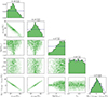 |
Fig. C.1. Posteriors on the hyperparameters controlling the variation in μm with redshift. Specifically, we show the asymptotic low-redshift peak location μm, low, the asymptotic high-redshift value μm, high, the logarithmic scale |


Similarly, Fig. C.2 shows our posterior on hyperparameters connected to redshift variation in the height fp of the Gaussian peak. We specifically show the posterior derived in Sec. 3.2, although these results are extremely similar to the analogous constraints on fp(z) derived in Sec. 3.1, as well as in Appendix D when varying all features in the black hole mass spectrum simultaneously. As discussed in the main text, the net change Δlog(fp) = fp, high−fp, low in the peak height with redshift is consistent with zero, although with a preference for positive values (a rising peak) over negative values (a shrinking peak). As was the case with μm(z) in Fig. C.1, any large changes in the peak height are generally required to occur over long scale lengths  We also include in Fig. C.2 the posterior on the slope αz with which the overall merger rate increases with redshift. This parameter is somewhat anti-correlated with Δlog(fp) = fp, high−fp, low. This is expected: in order to correctly predict the observed number of 35 M⊙ events at high redshifts without overpredicting the number of such events at low redshifts, the model can either posit that the overall merger rate grows with redshift (large αz and small Δfp), or adopt a constant merger rate but invoke a growing peak (small α and large Δfp).
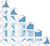 |
Fig. C.2. Various one-dimensional and two-dimensional posteriors of the hyperparameters in our analysis relating to the variation in fp in the power-law continuum are shown. The dark blue dashed lines in the one-dimensional distributions represent the priors. The hyperparameters shown here are the (ascending) power-law index αz of the modeled merger rate, and hyperparameters connected to varying fp from Eq. (2). This includes log(fp, low), log(fp, high), the width of the sigmoid |


The same broad features are present in Fig. C.3, which presents the posterior controlling the power-law slope of the primary mass spectrum. We again see a slight negative correlation between αlow and the ascending power-law index αz controlling growth of the overall merger rate. Large αz will generally overpredict the number of massive events at high redshift, unless compensated for by small Δα. Conversely, large Δα must in turn be compensated by small αz to guarantee less frequent massive mergers. We see a preference for higher values of the sigmoid width log(Δzα) and higher values of the difference Δα.
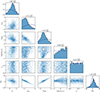 |
Fig. C.3. Posteriors of the hyperparameters related to the variation in α in redshift are shown. The dark blue dashed lines in the one-dimensional distributions represent the priors. The hyperparameters shown here are the (ascending) power-law index αz of the modeled merger rate, and then hyperparameters connected to varying α from Eq. (2). This includes αlow, αhigh, the width of the sigmoid log(Δzα) and the middle of the sigmoid |

In Sec. 4 we reversed our approach and instead investigated mass-dependence in the binary black hole redshift distribution. Figures C.4 and C.5 show posteriors on parameters governing mass evolution of the low-redshift slope αz of the merger rate and the peak redshift zp, respectively. Figure C.4 exhibits a significant amount of structure. Exactly as discussed above, we see an anticorrelation between the slope α of the black hole primary mass spectrum and any shifts Δαz in the growth of the merger rate as a function of mass. As illustrated in Fig. 6, the data also marginally favor positive Δαz, although Δαz = 0 remains quite consistent with observation. The posterior on the transition point  exhibits a somewhat striking peak near 33 M⊙ (this behavior too can be seen in Fig. 6); if there exists a transition in αz, it is likely to be centered at this location. This behavior, however, could simply be a consequence of the fact that a large number of observations occur near this mass, making this the point where αz(m1) is best constrained. Whether this posterior feature is real or just due to the relative underabundance of higher- and lower-mass events will require more data to determine. Figure C.5, in contrast, is relatively featureless, other than a preference against very low values of zp, low and zp, high.
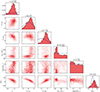 |
Fig. C.4. Posterior plots for varying the hyperparameters connected to αz. In this figure the power-law index of the primary mass distribution α, the four hyperparameters connected to the variation in αz via Eq. (2), and the posterior difference Δαz, are considered. |
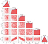 |
Fig. C.5. Posterior plots for all hyperparameters connected to the variation in zp in m1 are shown. The dashed lines denote the one-dimensional priors in the one-dimensional plots on top. The two-dimensional posteriors are shown in the corresponding row and column for the hyperparameters. Hyperparameters in this figure include the ascending power-law index αz, the four hyperparameters connected to varying zp via Eq. (2), and the difference between the high- and low-redshift value of zp. |
An alternative view of our results from Sec. 3.2 is given in Fig. C.6. In this figure, we show our posterior on the redshift-dependent merger rate (Eq. (13)) evaluated at three different primary mass values. The absolute merger rates in each panel reflect the overall shape of the mass distribution, which favors low-mass mergers, and uncertainties increase toward both higher masses and higher redshifts. At the same time, the merger rates in at each of the three masses are seen to rise in unison with one another, with no mass-dependent deviations.
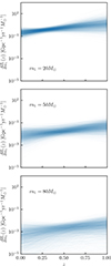 |
Fig. C.6. Three slices of the differential merger rate consisting out of the power-law analysis samples but viewed at a different m1 are shown. Above, we show m1 = 20 M⊙, in the middle m1 = 50 M⊙ and below m1 = 80 M⊙. |
Appendix D: Simultaneously varying the Gaussian peak and power-law continuum
In Secs. 3.1 and 3.2, we independently allowed the Gaussian peak and power-law components of the black hole primary mass spectrum to vary with redshift. For completeness, we have also repeated our analysis but simultaneously allowing all hyperparameters governing the black hole mass distribution to evolve with redshift.
When simultaneously varying both the Gaussian peak and the power-law continuum in this manner, results are unchanged relative to those presented in Sec. 3. In Fig. D.1, we show posteriors on the three most-informed parameters, the power-law slope and the Gaussian's mean and height, as a function of redshift. These posteriors exhibit the same trends identified in the main text above (compare with Figs. 3 and 5), with no requirement that any systematically vary with redshift. We also show in Fig. D.2 the corresponding posteriors on the primary mass distribution, as measured at redshifts z = 0.2 and z = 1; compare with Figs. 2 and 4, in which the Gaussian peak and power-law continuum are varied separately.
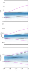 |
Fig. D.1. The traces of three hyperparameters from the all-varying analysis, where the blue lines are the sample traces, the dot-dashed black line is the median value of the traces, the solid black lines are the 95% confidence intervals and the magenta dotted lines are the conditional priors. The top panel shows the power-law continuum index α, the middle panel the location of the Gaussian excess μm and the bottom panel shows the fraction of events in the peak log fp. |
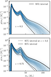 |
Fig. D.2. The primary mass distribution is shown for two different redshifts: z = 0.2 and z = 0.75, where the solid black lines show the 95% confidence intervals for the traces at that redshift, while the dashed black lines in the lower panel show the same lines but for z = 0.2 for visual comparison. |
All Tables
All Figures
|
Fig. 1. Cartoon illustrating the possible manners, as considered in this work, in which the primary mass distribution of a binary black hole might evolve with redshift. As illustrated in the left panel, we consider the possibilities that the location, width, and/or height of the 35 M⊙ excess evolve with redshift (see Sect. 3.1). As illustrated on the right, we allowed for the evolution of the height, slope, and endpoints of the power-law continuum (see Sect. 3.2). |
| In the text | |
|
Fig. 2. Inferred primary mass distribution of a binary black hole, when the Gaussian excess at ∼35 M⊙ evolves with redshift. Upper panel: Inferred primary mass distribution at z = 0.2. Green traces illustrate individual draws from our hyperposterior, and the solid black lines mark the 95% credible bounds. Lower panel: Primary mass distribution inferred at z = 0.75. For comparison, the dashed black lines illustrate the 95% credible bounds from the upper panel at z = 0.2. |
| In the text | |
|
Fig. 3. Inferred values of the hyperparameters characterizing the mean (top), standard deviation (middle), and height (bottom) of the Gaussian peak in the black hole mass spectrum as a function of redshift. In each panel, the green traces mark individual hyperposterior samples, and the solid and dot-dashed black curves indicate 95% credible posterior bounds and medians, respectively. The dashed cyan lines analogously illustrate 95% credible prior bounds. Finally, the dotted magenta curves indicate 95% credible prior bounds on each parameter when it is first conditioned on the measured posteriors at z = 0. |
| In the text | |
|
Fig. 4. As in Fig. 2, but the power-law continuum of the binary black hole primary mass spectrum evolves with redshift. |
| In the text | |
|
Fig. 5. As in Fig. 3, but showing posteriors on the redshift-dependent hyperparameters that characterize the power-law continuum. Specifically, we show posteriors on the power-law slope (top), mixing fraction (middle), and the location below which the mass distribution is truncated (bottom). The posteriors on other parameters (e.g. the maximum black hole mass and high- or low-mass truncation scales) are uninformative and are not shown here. |
| In the text | |
|
Fig. 6. Constraints on the power-law slope αz that governs the evolution of the volumetric binary black hole merger rate with redshift (top) and the peak redshift zp beyond which the merger rate turns over (bottom), each as as function of primary mass. As in Figs. 3 and 5, the black lines show the 95% credible posterior bounds, the dashed cyan lines mark prior bounds, and the dotted magenta curves illustrate prior bounds after they were conditioned on the best-measured posteriors at m1 = 35 M⊙. |
| In the text | |
|
Fig. C.1. Posteriors on the hyperparameters controlling the variation in μm with redshift. Specifically, we show the asymptotic low-redshift peak location μm, low, the asymptotic high-redshift value μm, high, the logarithmic scale |
| In the text | |
|
Fig. C.2. Various one-dimensional and two-dimensional posteriors of the hyperparameters in our analysis relating to the variation in fp in the power-law continuum are shown. The dark blue dashed lines in the one-dimensional distributions represent the priors. The hyperparameters shown here are the (ascending) power-law index αz of the modeled merger rate, and hyperparameters connected to varying fp from Eq. (2). This includes log(fp, low), log(fp, high), the width of the sigmoid |
| In the text | |
|
Fig. C.3. Posteriors of the hyperparameters related to the variation in α in redshift are shown. The dark blue dashed lines in the one-dimensional distributions represent the priors. The hyperparameters shown here are the (ascending) power-law index αz of the modeled merger rate, and then hyperparameters connected to varying α from Eq. (2). This includes αlow, αhigh, the width of the sigmoid log(Δzα) and the middle of the sigmoid |
| In the text | |
|
Fig. C.4. Posterior plots for varying the hyperparameters connected to αz. In this figure the power-law index of the primary mass distribution α, the four hyperparameters connected to the variation in αz via Eq. (2), and the posterior difference Δαz, are considered. |
| In the text | |
|
Fig. C.5. Posterior plots for all hyperparameters connected to the variation in zp in m1 are shown. The dashed lines denote the one-dimensional priors in the one-dimensional plots on top. The two-dimensional posteriors are shown in the corresponding row and column for the hyperparameters. Hyperparameters in this figure include the ascending power-law index αz, the four hyperparameters connected to varying zp via Eq. (2), and the difference between the high- and low-redshift value of zp. |
| In the text | |
|
Fig. C.6. Three slices of the differential merger rate consisting out of the power-law analysis samples but viewed at a different m1 are shown. Above, we show m1 = 20 M⊙, in the middle m1 = 50 M⊙ and below m1 = 80 M⊙. |
| In the text | |
|
Fig. D.1. The traces of three hyperparameters from the all-varying analysis, where the blue lines are the sample traces, the dot-dashed black line is the median value of the traces, the solid black lines are the 95% confidence intervals and the magenta dotted lines are the conditional priors. The top panel shows the power-law continuum index α, the middle panel the location of the Gaussian excess μm and the bottom panel shows the fraction of events in the peak log fp. |
| In the text | |
|
Fig. D.2. The primary mass distribution is shown for two different redshifts: z = 0.2 and z = 0.75, where the solid black lines show the 95% confidence intervals for the traces at that redshift, while the dashed black lines in the lower panel show the same lines but for z = 0.2 for visual comparison. |
| In the text | |
Current usage metrics show cumulative count of Article Views (full-text article views including HTML views, PDF and ePub downloads, according to the available data) and Abstracts Views on Vision4Press platform.
Data correspond to usage on the plateform after 2015. The current usage metrics is available 48-96 hours after online publication and is updated daily on week days.
Initial download of the metrics may take a while.