| Issue |
A&A
Volume 663, July 2022
|
|
|---|---|---|
| Article Number | A156 | |
| Number of page(s) | 8 | |
| Section | Stellar structure and evolution | |
| DOI | https://doi.org/10.1051/0004-6361/202243127 | |
| Published online | 26 July 2022 | |
The Gravitational Wave Universe Toolbox
II. Constraining the binary black hole population with second and third generation detectors
1
Department of Astrophysics/IMAPP, Radboud University, PO Box 9010 6500 GL Nijmegen, The Netherlands
e-mail: This email address is being protected from spambots. You need JavaScript enabled to view it.
2
Department of Mathematics/IMAPP, Radboud University, PO Box 9010 6500 GL Nijmegen, The Netherlands
3
SRON, Netherlands Institute for Space Research, Sorbonnelaan 2, 3584 CA Utrecht, The Netherlands
4
Institute of Astronomy, KU Leuven, Celestijnenlaan 200D, 3001 Leuven, Belgium
5
Key Laboratory of Particle Astrophysics, Institute of High Energy Physics, Chinese Academy of Sciences, 19B Yuquan Road, Beijing, 100049
PR China
Received:
17
January
2022
Accepted:
20
April
2022
Abstract
Context: The GW-Universe Toolbox is a software package that simulates observations of the gravitational wave (GW) Universe with different types of GW detectors, including Earth-based and space-borne laser interferometers and pulsar timing arrays. It is accessible as a website, and can also be imported and run locally as a Python package.
Methods: We employ the method used by the GW-Universe Toolbox to generate a synthetic catalogue of detection of stellar-mass binary black hole (BBH) mergers. As an example of its scientific application, we study how GW observations of BBHs can be used to constrain the merger rate as a function of redshift and masses. We study advanced LIGO (aLIGO) and the Einstein Telescope (ET) as two representatives of the second and third generation GW observatories, respectively. We also simulate the observations from a detector that is half as sensitive as the ET at its nominal designed sensitivity, which represents an early phase of the ET. We used two methods to obtain the constraints on the source population properties from the catalogues: the first uses a parameteric differential merger rate model and applies a Bayesian inference on the parameters; the other is non-parameteric and uses weighted Kernel density estimators.
Results: Our results show the overwhelming advantages of the third generation detector over those of the second generation for the study of BBH population properties, especially at redshifts higher than ∼2, where the merger rate is believed to peak. With the simulated aLIGO catalogue, the parameteric Bayesian method can still give some constraints on the merger rate density and mass function beyond its detecting horizon, while the non-parametric method loses the constraining ability completely there. The difference is due to the extra information placed by assuming a specific parameterisation of the population model in the Bayesian method. In the non-parameteric method, no assumption of the general shape of the merger rate density and mass function are placed, not even the assumption of its smoothness. These two methods represent the two extreme situations of general population reconstruction. We also find that, despite the numbers of detected events of the half ET can easily be compatible with full ET after a longer observation duration, and the catalogue from the full ET can still give much better constraints on the population properties due to its smaller uncertainties on the physical parameters of the GW events.
Key words: gravitational waves / methods: statistical / stars: black holes
© S.-X. Yi et al. 2022
 Open Access article, published by EDP Sciences, under the terms of the Creative Commons Attribution License (https://creativecommons.org/licenses/by/4.0), which permits unrestricted use, distribution, and reproduction in any medium, provided the original work is properly cited.
This article is published in open access under the Subscribe-to-Open model. This email address is being protected from spambots. You need JavaScript enabled to view it. to support open access publication.
1. Introduction
The era of gravitational wave (GW) astronomy began with the first detection of a binary black hole (BBH) merger in 2015 (Abbott et al. 2016). There have been ∼90 BBH systems discovered with ∼3 years of observations in the LIGO/Virgo O1/O2/O3 runs (GWTC-1 and -2 catalogues: Abbott et al. 2019b, 2021a). The number is catching up on that of discovered Galactic black holes (BHs) in X-ray binaries during the last half century (Corral-Santana et al. 2016). LIGO and Virgo are being upgraded towards their designed sensitivity, and new GW observatories such as The Kamioka Gravitational Wave Detector (KAGRA, Kagra Collaboration 2019) and LIGO-India (Iyer 2011) will join the network in the near future. Furthermore, there are plans for the next generation of GW observatories such as the Einstein Telescope (ET, Punturo et al. 2010) and the Cosmic Explorer (CE, Reitze et al. 2019), which will push forward the detecting horizon significantly. With the expected explosion in the size of the BBH population, the community has been actively studying what science can be extracted from GW observations of BBHs. Applications include for example the cosmic merger rate density of BBHs (e.g., Vitale et al. 2019), the mass distribution of stellar mass black holes (SMBHs; e.g., Kovetz 2017; Kovetz et al. 2017; Abbott et al. 2019a, 2021b), the rate of stellar nucleosynthesis (e.g., Farmer et al. 2020), and constraints on the expansion history of the Universe (Farr et al. 2019). Simulating a catalogue of observations was the crucial step in this latter work. In all literature mentioned above, the simulation is performed for specific detectors and observation duration and their catalogues are difficult to extend to other uses. Therefore, we are building a set of simulation tools that has the flexibility to be used with different detectors, observation durations, source populations, and cosmological models. The GW-Universe Toolbox is such a tool set; it simulates observations of the GW Universe (including populations of stellar-mass compact binary mergers, supermassive black hole binary inspirals and mergers, extreme-mass-ratio inspirals, etc.) with different types of GW detectors, including Earth-based and space-borne laser interferometers and pulsar timing arrays. It is accessible as a website1, or can be run locally as a Python package. For a detailed overview of the functionalities and methods of the GW-Universe Toolbox, please see Yi et al. (2021), which is referred to as Paper-I hereafter.
Here, we present one application of the GW-Universe Toolbox, showing how the cosmic merger rate and mass function of BHs can be constrained by GW observations using advanced LIGO (aLIGO, at design sensitivity) and ET. The current GW-Universe Toolbox can only simulate observations with single detectors. A network of detectors is expected to be more efficient in the following aspects: 1. the total S/N of a joint-observed GW source would be higher than (but of the same order of magnitude as) that from a single detector; 2. the uncertainties of source parameters would be smaller. In the current GW-Universe Toolbox, the duty cycle of detectors is assumed to be 100%. In a more realised simulation, where the duty cycles of single detectors are not 100%, a detector network also benefits from a longer time coverage. The cosmic merger rate density, or the volumetric merger rate as a function of redshift ℛ(z), provides valuable information on the history of the star formation rate (SFR), which is crucial for understanding the evolution of the Universe, for example in terms of chemical enrichment history, and the formation and evolution of galaxies (Madau & Dickinson 2014). The SFR as a function of redshift has been studied for decades mainly with UV, optical, and infrared observations of galaxies at different redshifts (Serjeant et al. 2002; Doherty et al. 2006; Thompson et al. 2006; Carilli et al. 2008; Magdis et al. 2010; Rujopakarn et al. 2010; Ly et al. 2011; Sedgwick et al. 2011; Kennicutt & Evans 2012; Curtis-Lake et al. 2013; Madau & Dickinson 2014). Such electromagnetic (EM) wave probes are limited by dust extinction, and the completeness of samples at high redshifts is difficult to estimate (e.g., Maiolino & Mannucci 2019). Moreover, the connection between the direct observable and the SFR history is model dependent on multiple layers (see e.g., Chruślińska et al. 2021). GWs provide a unique new probe that suffers less from the above-mentioned limitations.
Moreover, ℛ(z) depends also on the distribution of delay times τ, that is, the time lag between the formation of the binary massive stars and the merger of the two compact objects (e.g., Belczynski et al. 2010; Kruckow et al. 2018). Therefore, a combination of the SFR from EM observations and ℛ(z) from GW can improve our knowledge of the delay-time distribution. P(τ) together with the primary mass function p(m1) (where m1 is the mass of the primary BH) of BBHs helps us to better understand the physics in massive binary evolution, for example in the common envelope scenario (e.g., Belczynski et al. 2016; Kruckow et al. 2018).
There are several previous works that studied the prospect of using simulated GW observations to study ℛ(z) and p(m1) of BBH. Vitale et al. (2019) shows that with three months observation with a third-generation detector network, ℛ(z) can be constrained to high precision up to z ∼ 10. In their work, the authors did not take into account the signal-to-noise ratio (S/N) limits of detectors and instead made the assumption that all BBH mergers in the Universe are in the detected catalogue. Kovetz et al. (2017) studied how the observation with aLIGO can be used to give a constraint on p(m1). These authors assumed a certain parameterization of p(m1), and used an approximated method to obtain the covariance of the parameters based on a simulated catalogue of aLIGO observations. Recently, Singh et al. (2021) simulated observations with ET of compact object binary mergers, taking into account the effect of the rotation of the Earth. They found that ℛ(z) and mass distribution can be so well constrained from ET observations that mergers from different populations can be distinguished.
In this work, we simulate the observed catalogues of BBH mergers in ten years of aLIGO observations with its design sensitivity and one month of ET observations using the GW-Universe Toolbox. We also simulate the observation from a detector that is half as sensitive as the ET in design which represents the early phase of ET. The paper is organised as follows: In Sect. 2, we summarise the method used by the GW-Universe Toolbox to simulate the catalogue of BBH mergers; In Sect. 3, we use the synthetic catalogues to set constraints on the cosmic merger rate and mass function of the population. We employ two ways to constrain ℛ(z) along with the mass function of the primary BH. The first assumes parameteric forms of ℛ(z) and the mass function and uses Bayesian inference on their parameters. The other method does not assume a parameteric formula and uses weighted Kernel density estimators. The results are presented and compared. We conclude and discuss in Sect. 4.
2. Generating synthetic catalogues
2.1. Method
We use the GW-Universe Toolbox to simulate observations of a BBH with three different detectors, namely, aLIGO (designed sensitivity), ET, and ‘half-ET’2. The noise power spectrum Sn for aLIGO and ET are obtained from the LIGO website3. The ‘half-ET’ represents our expectation of the performance of the ET in its early phase. In Fig. 1, we plot the  as a function of frequency for aLIGO, ET at its designed sensitivity, and half-ET. For its Sn, we multiply Sn of the ET by a factor of 10.89 to obtain a noise curve that is half way between those of the designed aLIGO and ET. Here we give a brief summary of the method. For details, we refer to Yi et al. (2021). We first calculate a function 𝒟(z, m1, m2), which represents the detectability of a BBH with redshift z, and primary and secondary masses m1, m2. Here, 𝒟(z, m1, m2) depends on the antenna pattern and Sn of the detector, and the user designated S/N threshold. The other ingredient is the merger rate density distribution of BBH in the Universe, ṅ(z,m1,m2). In the GW-Universe Toolbox, we integrate two parameterized function forms for ṅ(z,m1,m2), namely pop-A and pop-B (see Yi et al. 2021 for the description on the population models). For a more sophisticated ṅ(z,m1,m2) from population synthesis simulations, see Belczynski et al. (2002), Mapelli et al. (2017, 2022), Mapelli & Giacobbo (2018), Arca Sedda et al. (2021), Banerjee (2022), van Son et al. (2022), Singh et al. (2021).
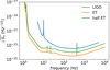 |
Fig. 1. Square-root of the noise power spectrum density of the aLIGO (blue) and ET (orange) at their designed sensitivity. The data used to make the plots were obtained from https://dcc.ligo.org/LIGO-T1800044/public and http://www.et-gw.eu/index.php/etsensitivities. |
The distribution of detectable sources, which we denote N(z, m1, m2), can be calculated with:
 (1)
(1)
where T is the observation duration, and Θ = (z, m1, m2). An integration of ND(Θ) gives the expectation of total detection number:
 (2)
(2)
The actual total number in a realization of the simulated catalogue is a Poisson random around this expectation. The synthetic catalogue of GW events is drawn from ND(Θ) with a Markov-chain Monte-Carlo (MCMC) algorithm.
We can also provide a rough estimation of the uncertainties on the intrinsic parameters of each event in the synthetic catalogue using the Fisher information matrix (FIM). Previous studies (e.g., Rodriguez et al. 2013) found that the FIM will sometimes severely overestimate the uncertainties, especially when the S/N is close to the threshold. We implement a correction whereby, if the relative uncertainty of masses calculated with FIM is larger than 20%, δm1, 2 = 0.2m1, 2 is applied instead.
The uncertainty of the redshift is in correlation with those of other external parameters, such as the localisation error. The actual localisation uncertainties are largely determined by the triangulation error of the detector network, which cannot yet be estimated with the current version of GW-Universe Toolbox. As a result, we do not have a reliable way to accurately estimate the errors on redshift. As an ad hoc method, we assign δz = 0.5z as a typical representative for the uncertainties of aLIGO, and δz = 0.017z + 0.012 as a typical representative for the uncertainties of ET (Vitale & Evans 2017). For half-ET, we assign δz = 0.1z + 0.01.
2.2. Catalogues
Using the above-mentioned method, we generate synthetic catalogues corresponding to 10 years of aLIGO observations, 1 month of ET observations, and 1 month of observations with half-ET. Figures 2–4 show events in those catalogues, along with the corresponding marginalised ND(Θ). The numbers in the catalogues are 2072, 1830, and 889, respectively. The catalogues agree with the theoretical number density, which proves the validity of the MCMC sampling process.
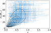 |
Fig. 2. aLIGO ten-year catalogue: black dashed lines are contours of ND(Θ) and blue points with error bars are 2072 events in the simulated catalogues. |
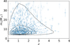 |
Fig. 3. ET one-month catalogue: black dashed lines are contours of ND(Θ) and blue points with error bars are 1830 events in the simulated catalogues. |
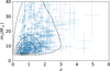 |
Fig. 4. Half-ET one-month catalogue: black dashed lines are contours of ND(Θ) and blue points with error bars are 889 events in the simulated catalogues. |
The underlying population model for ṅ(z,m1,m2) is pop-A, with parameters: Rn = 13 Gpc−3 yr−1, τ = 3 Gyr, μ = 3, c = 6, γ = 2.5, mcut = 95 M⊙, qcut = 0.4, σ = 0.1. Those parameters are chosen because they result in simulated catalogues which are compatible with the real observations (see Yi et al. 2021).
3. Constraints on ℛ(z) and p(m1) from BBH catalogues
In this section, we study how well ℛ and p(m1) can be constrained with BBH catalogues from observations with second and third generation GW detectors. Two distinct methods are used.
3.1. Bayesian method
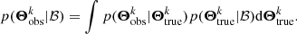
In the first method, we use a parameterised form of ṅ(Θ|ℬ). Here, ℬ are the parameters describing the population rate density, which are ℬ = (R0, τ, μ, c, γ, qcut, σ) in our case. Θk are the physical parameters of the k-th source in the catalogue, and we use {Θ} to denote the whole catalogue.
The posterior probability of ℬ given an observed catalogue {Θ}obs:
 (3)
(3)
where p({Θ}obs|ℬ) is the likelihood and p(ℬ) is the prior. The subscript ‘obs’ is to distinguish the observed parameters from the true parameters of the sources. Known as in an inhomogeneous Poisson Process, the likelihood of obtaining a catalogue {Θ}obs is the following (Foreman-Mackey et al. 2014):
 (4)
(4)
where p(N|λ(ℬ)) is the probability of detecting N sources if the expected total number is λ, which is a Poisson function. The probability of detecting a source k with parameters Θk is:
 (5)
(5)
We further assume that observational errors are Gaussian, and therefore we have p(Θobsk|Θtruek)=p(Θtruek|Θobsk). Taking this symmetric relation into Eq. (5), we have:
 (6)
(6)
The above integration is equivalent to the average of p(Θtruek|ℬ) over all possible Θk. Therefore,
 (7)
(7)
where the ⟨⋯⟩ denotes an average among a sample of Θk which is drawn from a multivariate Gaussian characterised by the observation uncertainties. Inserting Eq. (7) into Eq. (4), and noting that p(Θk|ℬ)≡ND(Θk|ℬ)/λ(ℬ), and p(N|λ(ℬ)) is the Poisson distribution,
 (8)
(8)
For the prior distribution p(ℬ), we use the log normal distributions for τ, R0, c, γ, and μ, which centre at the true values and the standard deviations are wide enough so that the posteriors are not influenced. The posterior probability distributions of the parameters are obtained with MCMC sampling from the posterior in Eq. (3). We keep the nuisance parameters qcut and σ fixed to the true value, in order to reduce the necessary length of the chains. The posterior of the interesting parameters would not be influenced significantly by leaving these free.
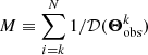
In Fig. 5, we plot the MCMC chains sampled from the posterior distribution of the population parameters, where we can see the chains are well mixed, and thus can serve as a good representation of the underlying posterior distribution. In Fig. 6, we plot the correlation between the parameters of the redshift dependence (Rn, τ) and those between the parameters of the mass function (μ, c, γ). We find strong correlations between the ℛ(z) parameters τ and Rn, and also among the p(m1) parameters γ, c, and μ. The correlation between parameters of the redshift dependence and those of the mass function are small and therefore not plotted.
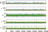 |
Fig. 5. MCMC chains sampled from the posterior distribution of the population parameters. The blue line is for the 10 yr of aLIGO observations, the green line is for the month of observations with half-ET, and the orange line is for the month of observations with full ET. The black dashed lines mark the true values of the corresponding parameters, which were used to generate the observed catalogue. |
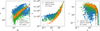 |
Fig. 6. Correlation between the parameters of redshift dependence (Rn, τ, left panel) and among the parameters of mass function (μ, c, γ, middle and right panel). Blue markers correspond to 10 yr of observations with aLIGO; green markers correspond to 1 month of observations with half-ET, and orange markers correspond to 1 month of observations with ET. The red cross in each panel marks the location of the true values that were used to generate the observed catalogue. |
In Fig. 7, we plot the inferred differential merger rate as a function of redshift and mass of the primary BH. The bands correspond to the 95% confidence level of the posterior distribution of the population parameters. We can see from the panels of Fig. 7 that, although 10 yr of aLIGO observations and 1 month of ET observations result in a similar number of detections, ET can still obtain much better constraints on both ℛ(z) and p(M1). This is due to (1): the much smaller uncertainties on parameters with ET observations compared to those with aLIGO, and (2) the fact that the catalogue produced from observations with ET covers larger ranges in redshift and mass than that of aLIGO. For half-ET and ET, at low redshift and high mass, the two detectors result in a similar number of detections, and therefore they give comparable constraints on ℛ(z) at low redshift and p(m1) at large mass. On the other hand, at high redshift and low mass, the full ET observed more events and with lower uncertainties, and therefore gives better constraints than that of half-ET.
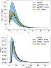 |
Fig. 7. ℛ(z) (upper panel) and p(m1) (lower panel) reconstructed with the Bayesian method from the synthetic aLIGO (blue), ET (orange), and half-ET (green) catalogues. The black dashed curves show the models used to generate the catalogues. |
We see from Fig. 2 that the maximum redshift in the aLIGO catalogue is z ∼ 1.5, while ℛ(z) can still be constrained for z > 1.5, and can even be more stringent towards larger redshift. This constraint on ℛ(z) at large redshift is not from the observed catalogue, but is intrinsically imposed by the assumed model in the Bayesian method: we fixed our star formation rate as a function of redshift so that ψ(zf) peaks at z ∼ 2. The peak of the BBH merger rate can therefore only appear later.
3.2. Non-parametric method
From Eq. (1), we know that
 (9)
(9)
and ND(Θ) can be inferred from the observed catalogue.
Marginalising over m1 and m2 in Eq. (9) on both sides, we have
 (10)
(10)
where I(z) is the 1D intensity function (number density) over z calculated from the observed catalogue, with weights wi equal to the corresponding 1/𝒟(Θi). The intensity can be calculated with an empirical density estimator of the (synthetic) catalogue or with the (non-normalised) weighted kernel density estimator (KDE; see Appendix A). By simulating a number of different realisations of the Universe population inferred from I(z), the confidence intervals of the estimated I(z) are obtained.
Here, in order to include the observational uncertainties and give at the same time an estimate of the confidence intervals of the KDE, a specific bootstrap is employed, as follows:
The GW-Universe Toolbox returns a catalogue {Θ}true, where Θtruek denotes the true parameters of the kth events in the catalogue, including its m1, m2, and z, and their uncertainties δm1, δm2, and δz. Here, k goes from 1 to N, where N is the total number of events.
Shift the true values Θtruek according to a multivariate Gaussian centred on the true values and with covariance matrix given by the corresponding uncertainties. Therefore, a new catalogue {Θk}obs is obtained.
Estimate the detection probabilities 𝒟(Θobsk).
Calculate the (non-normalized) weighted KDE of {Θobsk}, with weights 1/𝒟(Θobsk). The intensity is estimated on the log and then transformed back to the original support; this ensures that there is no leakage of the intensity on negative support.
Take
 as an estimate of the total number of mergers in the Universe in the parameter space.
Generate a realisation
 according to a Poisson with expected value M.
Draw a sample of size
 from the KDE calculated in step 4. This is the equivalent of generating a new Universe sample based on the estimate of the distribution in the Universe from the observations.
For each of the events in the above sample, calculate its detection probability. Draw
 uniform random values, U, in between 0 and 1, and drop the observations for whose detectability is less than U. A smaller sample is left, which represents a new realisation of the detected catalogue.
Estimate the covariance for each observation of the generated data set ΣΘk using interpolation of the original catalogue, and shift them according to a multivariate Gaussian centred on each observation and with covariance matrix ΣΘk.
Estimate their detection probability.
Calculate the (non-normalized) weighted KDE of the above mentioned sample.
Repeat steps from 6 to 11 for a large number of times B (we find B = 200 is large enough). Calculate the confidence intervals according to the assigned quantiles.
Based on the results above, we can correct for the bias introduced by the measurement uncertainties. We estimate the bias between the bootstrap intensities and the intensity estimated on the observed sample, and use it to rescale the estimated intensity of the observed sample.
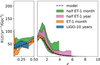 |
Fig. 8. Merger rate as function of the redshift, reconstructed with Eq. (11) from the synthetic aLIGO, ET, and half-ET catalogues. |
Similarly, the merger rate in the Universe as a function of the mass of the primary BH is
 (11)
(11)
where p(m1) is the normalised mass function of the primary BH, ṅtot is the total number of BBH mergers in the Universe in a unit local time, and I(m1) is the 1D intensity function of m1, calculated from the observed catalogue. The procedure for obtaining I(m1) is the same as that used to calculate I(z).
Figures 8 and 9 show the ℛ(z) and ℛ(m1) reconstructed with Eqs. (10) and (11) from the synthetic aLIGO, ET, and half-ET catalogues. The shaded areas are the 95% confidence intervals.
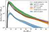 |
Fig. 9. Merger rate as a function of the primary BH mass, reconstructed with Eq. (11) from the synthetic aLIGO, ET, and half-ET catalogues. |
We note in Fig. 8 that, for aLIGO observations, the obtained ℛ(z) in z > 0.3 is an underestimate of the underlying model. This is because the aLIGO detectable range of BBH masses is increasingly incomplete towards higher redshift. An intuitive illustration is shown in Fig. 10. There, we plot the 2D merger rate density as a function of m1 and z. The underlying black region marks the parameter space region where the detectability is essentially zero, which is the region beyond aLIGO’s horizon. When plotting Fig. 10, we set the cut to 𝒟(z, m1, m2 = m1)< 10−2. We can see the fraction of the black region in the mass spectrum is increasing towards high redshift. This corresponds to the fact that BBH with small masses cannot be detected with aLIGO at higher redshift.
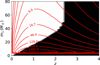 |
Fig. 10. Two-dimensional theoretical merger rate as a function of redshift and primary masses. The black region marks the region in the parameter space that is not reachable by aLIGO (single aLIGO detector at its nominal sensitivity). |
Similarly, in Fig. 9, we see ℛ(m1) is deviating the theory towards low m1. To compare the estimation with the model, we limit both the aLIGO catalogue and the theory in the range z < 0.6. Therefore, the meaning of ℛ(m1) is no longer the merger rate density of the complete Universe, but that of a local Universe up to 0.6, which is calculated with:
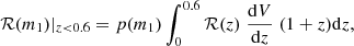 (12)
(12)
where p(m1) is the normalised mass function.
The result is unlike the results with the Bayesian inference method, where constraints can still be placed in regimes with no detection. The constraints on ℛ(z) and the mass function are also less tight from the non-parametric method compared with those calculated using the parametric one. The difference is rooted in the degree of prior knowledge we assume with the population model in both methods: In the parametric method, we assume the function forms which are exactly the same as the underlying population model that was used to generate the simulated catalogue. This represents an overly optimistic extreme, because in reality, we would never be able to guess a perfect function representation of the underlying population. On the other hand, in the non-parametric method, we do not impose any assumption on the properties of the population model. This represents a conservative extreme, because in reality, we have a good idea of the general shape or trends of the population.
4. Conclusion and discussion
In this paper, we describe the details of how the GW-Universe Toolbox simulates observations of BBH mergers with different ground-based GW detectors. As a demonstration of its scientific application, we use synthetic catalogues produced using this software to reconstruct and constrain the cosmic merger rate and mass function of the BBH population. The comparison amongst the results from 1 month of (half) ET observations and 10 yr of aLIGO observations reveals the overwhelming advantages of the third generation detectors over those of the second generation, especially at redshifts higher than ∼2, which is approximately where the cosmic merger rate is believed to peak.
The reconstruction and constraint of ℛ(z) and p(m1) are performed with two methods, namely (1) a Bayesian method, assuming a parameteric formula of ℛ(z) and p(m1), and (2) a KDE method with non-parameteric ℛ(z) and p(m1). For the catalogue of ET observations, the results from both methods are qualitatively the same. However, for aLIGO, the Bayesian method can put constraints on ℛ(z) beyond the detecting limit, where the non-parameteric method loses its ability completely. The m1 dependence is also much more accurately reconstructed by the Bayesian method than the non-parameteric method for the aLIGO catalogue. The difference is due to the extra information placed by assuming a specific parameterisation of the population model in the Bayesian method. In our example, the underlying ℛ(z) and p(m1) used to generate the catalogues are the same as those assumed in the Bayesian method; while in the KDE method, no assumptions are made of the general shape of ℛ(z) and f(m1), not even of its smoothness. These represent the two extreme situations in the differential merger rate reconstruction.
In reality, the underlying shapes of ℛ(z) and f(m1) are unknown and they could be very different from those used here. The parameterised Bayesian method may give biased inference and underestimated uncertainties. Furthermore, any unexpected structures in ℛ(z) and f(m1) cannot be recovered with the parameterised Bayesian method. For instance, there can be additional peaks in the BH spectrum corresponding to pulsational pair-instability supernovae and primordial BHs. On the other hand, although the function form of the merger rate is unknown, the general trends should be more or less known. A better reconstruction method should lie in between these two extreme methods.
An alternative method is to parameterise ℛ(z) and p(m1) as piecewise constant functions and use the Bayesian inference to obtain the posterior of the values in each bin, as in Vitale et al. (2019). This confers the advantage that no assumptions on the shapes of ℛ(z) and p(m1) are needed, as in the Kernel density estimator method. The disadvantage of this method is that MCMC sampling in high dimensions needs to be performed. If one assumes that p(m1) is independent of z, there are more than N + M free parameters, where N and M are the number of bins in z and m1 respectively. If we want the resolutions to be 0.5 in z and 1 M⊙ in m1, then the dimension of the parameter space is > 80 for the ET catalogue. In the more general case, when one includes the dependence of p(m1) on z, the number of parameters becomes N × M, and therefore the dimension of the parameter space goes to > 1200.
Another conclusion we draw about the early-phase ET (half-ET) is that it can also give a good constraint on ℛ(z) for high-redshift Universe. However, both ℛ(z) and the primary mass function are less accurately constrained than they are when using the full ET, even using a larger number of detected events from a longer observation duration. This is because the full ET determines smaller uncertainties on the physical parameters of the GW events.
In this paper, we compare the results from a single aLIGO detector with that of ET. In reality, there will always be multiple detectors working as a network (e.g., LIGO-Virgo-KAGRA), which is expected to lead to better results than those provided by a single aLIGO. However, we do not expect a qualitatively different conclusion from what we find here, namely that the ET (as a representative of the third generation GW detectors) has an overwhelming greater ability to constrain the BBH population properties than the second generation detectors, even when these latter are used in the form of a network. We anticipate that the same conclusion applies to other third generation GW detectors, for example the Cosmic Explorer.
Here we are referring to the ET-D design. For the key parameters of this ET configuration; see Hild et al. (2011).
Acknowledgments
We thank the reviewer for his/her useful suggestions to improve the manuscript. G. Nelemans thanks the support from the Dutch National Science Agenda, NWA Startimpuls – 400.17.608 on the GW-Universe Toolbox project.
References
- Abbott, B. P., Abbott, R., Abbott, T. D., et al. 2016, Phys. Rev. Lett., 116, 061102 [Google Scholar]
- Abbott, B. P., Abbott, R., Abbott, T. D., et al. 2019a, Phys. Rev. X, 9, 031040 [Google Scholar]
- Abbott, B. P., Abbott, R., Abbott, T. D., et al. 2019b, ApJ, 882, L24 [Google Scholar]
- Abbott, R., Abbott, T. D., Abraham, S., et al. 2021a, Phys. Rev. X, 11, 021053 [Google Scholar]
- Abbott, R., Abbott, T. D., Abraham, S., et al. 2021b, ApJ, 913, L7 [NASA ADS] [CrossRef] [Google Scholar]
- Arca Sedda, M., Mapelli, M., Benacquista, M., et al. 2021, MNRAS, submitted, [arXiv:2109.12119] [Google Scholar]
- Banerjee, S. 2022, Phys. Rev. D, 105, 023004 [NASA ADS] [CrossRef] [Google Scholar]
- Belczynski, K., Kalogera, V., & Bulik, T. 2002, ApJ, 572, 407 [NASA ADS] [CrossRef] [Google Scholar]
- Belczynski, K., Dominik, M., Bulik, T., et al. 2010, ApJ, 715, L138 [Google Scholar]
- Belczynski, K., Holz, D. E., Bulik, T., et al. 2016, Nature, 534, 512 [NASA ADS] [CrossRef] [Google Scholar]
- Carilli, C. L., Lee, N., Capak, P., et al. 2008, ApJ, 689, 883 [NASA ADS] [CrossRef] [Google Scholar]
- Chruślińska, M., Nelemans, G., Boco, L., et al. 2021, MNRAS, 508, 4994 [CrossRef] [Google Scholar]
- Corral-Santana, J. M., Casares, J., Muñoz-Darias, T., et al. 2016, A&A, 587, A61 [NASA ADS] [CrossRef] [EDP Sciences] [Google Scholar]
- Curtis-Lake, E., McLure, R. J., Dunlop, J. S., et al. 2013, MNRAS, 429, 302 [NASA ADS] [CrossRef] [Google Scholar]
- DiNardo, J., Fortin, N., & Lemieux, T. 1996, Econometrica, 64, 1001 [CrossRef] [Google Scholar]
- Doherty, M., Bunker, A., Sharp, R., et al. 2006, MNRAS, 370, 331 [NASA ADS] [CrossRef] [Google Scholar]
- Farr, W. M., Fishbach, M., Ye, J., et al. 2019, ApJ, 883, L42 [NASA ADS] [CrossRef] [Google Scholar]
- Farmer, R., Renzo, M., de Mink, S. E., et al. 2020, ApJ, 902, L36 [CrossRef] [Google Scholar]
- Foreman-Mackey, D., Hogg, D. W., & Morton, T. D. 2014, ApJ, 795, 64 [Google Scholar]
- Hild, S., Abernathy, M., Acernese, F., et al. 2011, CQG, 28, 094013 [NASA ADS] [CrossRef] [Google Scholar]
- Iyer, B., et al. 2011, https://dcc.ligo.org/LIGO-M1100296/public [Google Scholar]
- Kagra Collaboration (Akutsu, T., et al.) 2019, Nat. Astron., 3, 35 [NASA ADS] [CrossRef] [Google Scholar]
- Kennicutt, R. C., & Evans, N. J. 2012, ARA&A, 50, 531 [NASA ADS] [CrossRef] [Google Scholar]
- Kovetz, E. D. 2017, Phys. Rev. Lett., 119, 131301 [NASA ADS] [CrossRef] [Google Scholar]
- Kovetz, E. D., Cholis, I., Breysse, P. C., et al. 2017, Phys. Rev. D, 95, 103010 [NASA ADS] [CrossRef] [Google Scholar]
- Kruckow, M. U., Tauris, T. M., Langer, N., et al. 2018, MNRAS, 481, 1908 [CrossRef] [Google Scholar]
- Ly, C., Lee, J. C., Dale, D. A., et al. 2011, ApJ, 726, 109 [Google Scholar]
- Madau, P., & Dickinson, M. 2014, ARA&A, 52, 415 [Google Scholar]
- Maiolino, R., & Mannucci, F. 2019, A&ARv, 27, 3 [Google Scholar]
- Magdis, G. E., Elbaz, D., Daddi, E., et al. 2010, ApJ, 714, 1740 [NASA ADS] [CrossRef] [Google Scholar]
- Mapelli, M., & Giacobbo, N. 2018, MNRAS, 479, 4391 [NASA ADS] [CrossRef] [Google Scholar]
- Mapelli, M., Giacobbo, N., Ripamonti, E., et al. 2017, MNRAS, 472, 2422 [NASA ADS] [CrossRef] [Google Scholar]
- Mapelli, M., Bouffanais, Y., Santoliquido, F., et al. 2022, MNRAS, 511, 5797 [NASA ADS] [CrossRef] [Google Scholar]
- Punturo, M., Abernathy, M., Acernese, F., et al. 2010, CQG, 27, 194002 [NASA ADS] [CrossRef] [Google Scholar]
- Reitze, D., Adhikari, R. X., Ballmer, S., et al. 2019, Bull. Am. Astron. Soc., 51, 35 [Google Scholar]
- Rujopakarn, W., Eisenstein, D. J., Rieke, G. H., et al. 2010, ApJ, 718, 1171 [NASA ADS] [CrossRef] [Google Scholar]
- Rodriguez, C. L., Farr, B., Farr, W. M., et al. 2013, Phys. Rev. D, 88, 084013 [NASA ADS] [CrossRef] [Google Scholar]
- Singh, N., Bulik, T., Belczynski, K., et al. 2021, ArXiv e-prints [arXiv:2112.04058] [Google Scholar]
- Scott, D. W. 1992, Multivariate Density Estimation: Theory, Practice and Visualization (New York: John Wiley& Sons Inc) [CrossRef] [Google Scholar]
- Scott, D. W., & Terrell, G. R. 1987, J. Am. Stat. Assoc., 82, 1131 [CrossRef] [Google Scholar]
- Sedgwick, C., Serjeant, S., Pearson, C., et al. 2011, MNRAS, 416, 1862 [NASA ADS] [CrossRef] [Google Scholar]
- Serjeant, S., Gruppioni, C., & Oliver, S. 2002, MNRAS, 330, 621 [NASA ADS] [CrossRef] [Google Scholar]
- Silverman, B. W. 1986, Chapman and Hall/CRC [Google Scholar]
- Thompson, R. I., Eisenstein, D., Fan, X., et al. 2006, ApJ, 647, 787 [NASA ADS] [CrossRef] [Google Scholar]
- van Son, L. A. C., de Mink, S. E., Callister, T., et al. 2022, ApJ, 931, 17 [NASA ADS] [CrossRef] [Google Scholar]
- Vitale, S., & Evans, M. 2017, Phys. Rev. D, 95, 064052 [NASA ADS] [CrossRef] [Google Scholar]
- Vitale, S., Farr, W. M., Ng, K. K. Y., et al. 2019, ApJ, 886, L1 [NASA ADS] [CrossRef] [Google Scholar]
- Yi, S. X., Nelemans, G., Brinkerink, C., et al. 2021, https://doi.org/10.1051/0004-6361/202141634 (Paper I) [Google Scholar]
Appendix A: Kernel density estimation
Kernel density estimation (KDE) is one of the most famous methods for density estimation. For the univariate case, KDE is defined as:
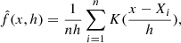 (A.1)
(A.1)
where K is the chosen kernel and h is the so-called bandwidth parameter. In the case of a Gaussian kernel, h can be thought of as the standard deviation of the normal density centred on each data point. The choice of the kernel does not significantly affect the density estimate if the number of observations is high enough; however, the choice of the bandwidth parameter h does affect the estimate, and has to be estimated with one of the available methods. The most common methods are rule-of-thumb, as in Scott’s rule (Scott 1992): H = n−2/(m + 4)Σ, and Silverman’s rule (Silverman 1986): 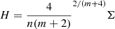 , where m is the number of the variables, n is the sample size, and Σ is the empirical covariance matrix. A more accurate but computationally expensive method is cross-validation bandwidth selection described in Scott & Terrell (1987).
As introduced in DiNardo et al. (1996), KDE can be adapted to the case where each observation is attached to a weight that reflects its contribution to the sample. The weighted kernel density estimator can be written as
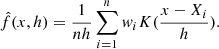 (A.2)
(A.2)
To ensure that the result of the density estimation still has the properties of a density, it is necessary to normalise the weights so that  .
.
KDE is easily extendable to the multivariate case, and used to estimate densities f in Rp based on the same principle: perform an average of densities centred at the data points. For the multivariate case, KDE is defined as:
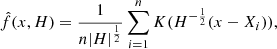 (A.3)
(A.3)
where K is the multivariate kernel, a p-variate density that depends on the bandwidth matrix H, a p × p symmetric and positive definite matrix.
All Figures
|
Fig. 1. Square-root of the noise power spectrum density of the aLIGO (blue) and ET (orange) at their designed sensitivity. The data used to make the plots were obtained from https://dcc.ligo.org/LIGO-T1800044/public and http://www.et-gw.eu/index.php/etsensitivities. |
| In the text | |
|
Fig. 2. aLIGO ten-year catalogue: black dashed lines are contours of ND(Θ) and blue points with error bars are 2072 events in the simulated catalogues. |
| In the text | |
|
Fig. 3. ET one-month catalogue: black dashed lines are contours of ND(Θ) and blue points with error bars are 1830 events in the simulated catalogues. |
| In the text | |
|
Fig. 4. Half-ET one-month catalogue: black dashed lines are contours of ND(Θ) and blue points with error bars are 889 events in the simulated catalogues. |
| In the text | |
|
Fig. 5. MCMC chains sampled from the posterior distribution of the population parameters. The blue line is for the 10 yr of aLIGO observations, the green line is for the month of observations with half-ET, and the orange line is for the month of observations with full ET. The black dashed lines mark the true values of the corresponding parameters, which were used to generate the observed catalogue. |
| In the text | |
|
Fig. 6. Correlation between the parameters of redshift dependence (Rn, τ, left panel) and among the parameters of mass function (μ, c, γ, middle and right panel). Blue markers correspond to 10 yr of observations with aLIGO; green markers correspond to 1 month of observations with half-ET, and orange markers correspond to 1 month of observations with ET. The red cross in each panel marks the location of the true values that were used to generate the observed catalogue. |
| In the text | |
|
Fig. 7. ℛ(z) (upper panel) and p(m1) (lower panel) reconstructed with the Bayesian method from the synthetic aLIGO (blue), ET (orange), and half-ET (green) catalogues. The black dashed curves show the models used to generate the catalogues. |
| In the text | |
|
Fig. 8. Merger rate as function of the redshift, reconstructed with Eq. (11) from the synthetic aLIGO, ET, and half-ET catalogues. |
| In the text | |
|
Fig. 9. Merger rate as a function of the primary BH mass, reconstructed with Eq. (11) from the synthetic aLIGO, ET, and half-ET catalogues. |
| In the text | |
|
Fig. 10. Two-dimensional theoretical merger rate as a function of redshift and primary masses. The black region marks the region in the parameter space that is not reachable by aLIGO (single aLIGO detector at its nominal sensitivity). |
| In the text | |
Current usage metrics show cumulative count of Article Views (full-text article views including HTML views, PDF and ePub downloads, according to the available data) and Abstracts Views on Vision4Press platform.
Data correspond to usage on the plateform after 2015. The current usage metrics is available 48-96 hours after online publication and is updated daily on week days.
Initial download of the metrics may take a while.