| Issue |
A&A
Volume 691, November 2024
|
|
|---|---|---|
| Article Number | A238 | |
| Number of page(s) | 12 | |
| Section | Extragalactic astronomy | |
| DOI | https://doi.org/10.1051/0004-6361/202451374 | |
| Published online | 18 November 2024 | |
Projections of the uncertainty on the compact binary population background using popstock
1
Dipartimento di Fisica G. Occhialini, Universitá degli Studi di Milano-Bicocca, Piazza della Scienza 3, 20126 Milano, Italy
2
INFN, Sezione di Milano-Bicocca, Piazza della Scienza 3, 20126 Milano, Italy
3
Department of Physics, California Institute of Technology, Pasadena, California 91125, USA
⋆ Corresponding author; This email address is being protected from spambots. You need JavaScript enabled to view it.
Received:
4
July
2024
Accepted:
18
September
2024
Abstract
The LIGO-Virgo-KAGRA collaboration has announced the detection to date of almost 100 binary black holes that have been used in several studies to infer the features of the underlying binary black hole population. From these objects it is possible to predict the overall gravitational-wave (GW) fractional energy density contributed by black holes throughout the Universe, and thus estimate the gravitational-wave background (GWB) spectrum emitted in the current GW detector band. These predictions are fundamental in our forecasts for background detection and characterisation, with both present and future instruments. The uncertainties in the inferred population strongly impact the predicted energy spectrum, and in this paper we present a new flexible method to quickly calculate the energy spectrum for varying black hole population features, such as the mass spectrum and redshift distribution. We have implemented this method in an open-access package, popstock, and extensively tested its capabilities. Using popstock, we investigated how uncertainties in these distributions impact our detection capabilities, and present several caveats for background estimation. In particular, we find that the standard assumption that the background signal follows a two-thirds power law at low frequencies is both waveform and mass-model dependent, and that the power-law signal is likely shallower than previously modelled, given the current waveform and population knowledge.
Key words: black hole physics / gravitational waves / cosmology: miscellaneous
© The Authors 2024
 Open Access article, published by EDP Sciences, under the terms of the Creative Commons Attribution License (https://creativecommons.org/licenses/by/4.0), which permits unrestricted use, distribution, and reproduction in any medium, provided the original work is properly cited.
This article is published in open access under the Subscribe to Open model. This email address is being protected from spambots. You need JavaScript enabled to view it. to support open access publication.
1. Introduction
The Laser Interferometer Gravitational-wave Observatory (LIGO) (Aasi et al. 2015), Virgo (Acernese et al. 2015), and KAGRA (Akutsu et al. 2019) detectors are progressively uncovering the features of the population of merging stellar-mass binary black holes in our Universe (Abbott et al. 2021a, 2023a). As observing runs become more and more sensitive, the detection horizon increases and a higher number of gravitational-wave (GW) events are positively identified as binary mergers. The events observed so far lie at distances z ≲ 1 (Abbott et al. 2023b), while the vast majority of binary mergers are expected to lie well beyond this horizon, as suggested by both theoretical expectations for the merger rate redshift evolution (Dominik et al. 2015; Belczynski et al. 2016; Rodriguez et al. 2018) and its inferred trend from GW data through the Third Gravitational-Wave Transient Catalogue (GWTC-3) Abbott et al. (2023a). This knowledge has motivated studies and the inference of the sub-threshold unresolved collection of binaries, treated as an overall gravitational-wave background (GWB) signal.
Works forecasting the GWB from compact binaries populate the literature. Before the first GW detections, these were based on theoretical models of the binary population (Phinney 2001; Regimbau 2007, 2011), while more recently GW data-informed projections (Abbott et al. 2021c) have become a benchmark for the GW community. An important distinction to make is between estimates of a specific realisation of the background, for example used in mock-data challenges (Meacher et al. 2014), and estimates of the ensemble average of the background, which corresponds to the expectation value of the background amplitude targeted by GWB searches (Zhu et al. 2011; Wu et al. 2012). In both cases, the calculation involves the (expected) distributions for the individual binary parameters, such as mass, distance, and event rate distributions. These population models are often taken to be simple parametric functions with a well-defined set of hyperparameters, which are fixed to fiducial (or assumed) values for the background calculation. Recalculating the background signal for varying population hyperparameters can become computationally intensive when employing large sample sets.
Several applications in the literature require marginalising the background signal over possible population configurations, including forecasting studies, such as those presented by the LIGO-Virgo-KAGRA (LVK) collaboration in Abbott et al. (2021c) and Abbott et al. (2023a), and inference analyses in Callister et al. (2020), Abbott et al. (2021c), and Turbang et al. (2024), among others. As the interest in this type of work grows, there is a need for efficient and flexible background estimation procedures. In this paper we present a method to efficiently carry out these calculations, called popstock, that we have made available to the community as an open-access code base. The novelty of our approach is in the design of a reweighting technique that allows us to sample the binary parameter probability distributions and evaluate a corresponding set of waveform approximants only once, enabling an extremely efficient re-estimation of the GWB when varying population hyperparameters. An analogous reweighting approach was previously implemented in Turbang et al. (2024). Furthermore, we implement the use of waveform templates imported from the LIGO Scientific Collaboration Algorithm Library (LAL) LIGO Scientific Collaboration (2020). To improve efficiency, previous codes have employed analytic waveform approximations directly embedded in the codebase; with our CPU-optimised spectral calculations and our GPU-optimised reweighting technique, we are able to support a much broader range of waveforms through the commonly used Python library for GW analysis, Bilby (Ashton et al. 2019).
We used popstock to investigate the impact of the uncertainty on the binary population on the detection prospects of the GWB with ground-based interferometers. In particular, we made a comparison with and extended the work done in Abbott et al. (2023a) to include more uncertainties on the redshift distribution of sources. We also employed the package to probe the effect of waveform choice on the estimation, and whether this is entirely degenerate with the population uncertainty. We find that the expected background amplitude can be significantly boosted when admitting higher mass mergers and higher rates of mergers at low redshift, within current population uncertainties. We further find that the choice of waveform can have noteworthy effects on background signal estimates; however, these do not dominate the current population uncertainties.
This paper is organised as follows. In Sect. 2 we introduce the theoretical aspects behind compact binary GWB calculations. In Sect. 3 we define the analytic models used here to describe the distributions of black hole masses and distances. In Sect. 4 we introduce popstock, our new package for GWB calculations, outlining its key functionalities. In Sect. 5 we present our background calculations and investigations, and finally we summarise our conclusions in Sect. 6.
2. The compact binary GW background
The amplitude of the GWB signal is parametrised by the fractional energy density spectrum emitted by GWs throughout the Universe, ΩGW(f) (Phinney 2001),
 (1)
(1)
which is normalised by the critical energy density of the Universe ρc = 3c2H02/8πG. This is in general the total energy density contributed by GWs throughout the Universe, and is not restricted to sub-threshold signals. Calculating a residual background requires the definition of a detection cutoff, which is detector-dependent1, while here and elsewhere ΩGW is considered to be an astrophysical property of the Universe.
While the GWB spectrum is detector-independent, it is useful to employ the detector frame to perform calculations. This allows us to immediately relate the intrinsic signal amplitude with the measured signal in GW detectors. As shown for example in Meacher et al. (2015), and Regimbau (2022), the energy density spectrum ΩGW(f) may be estimated as the average fractional GW energy density present in a detector during an observation time Tobs,
 (2)
(2)
assuming a finite number of GWs received at the detector, Ni. Here 𝒫d(Θi, f) is the Fourier domain unpolarised power in the detector frame (hence the subscript d) associated with a GW with parameters Θi, defined as
 (3)
(3)
where  is the Fourier transform of the GW waveform evaluated at Θi
2. So defined, 𝒫d has units s−2.
is the Fourier transform of the GW waveform evaluated at Θi
2. So defined, 𝒫d has units s−2.
In the limit of infinite observation time and infinite events, the ΩGW spectrum approaches its ensemble average,  . While the ΩGW measured by an experiment depends on the specific realisation observed throughout the experiment observation time,
  only depends on the distributions that describe the GW parameters Θ, which are in turn parametrised via population hyperparameters Λ (Phinney 2001). The
  spectrum is thus a unique population signature, and is targeted in observations in practice by measuring ΩGW for large Tobs. The equivalence is easily seen in the limit of large GW numbers as
 (4)
(4)
where pd(Θ|Λ) are the (normalised) detector frame probability distributions for the GW parameters Θ, such that
 (5)
(5)
Here  is the total rate of events per unit detector-frame time. It can be convenient to isolate the redshift integral in Eq. (5), assuming redshift is independent from other parameters, and to incorporate the rate in the redshift evolution probability p(z), defining the event rate per unit detector-frame time per redshift shell:
 (6)
(6)
The  spectrum can then be interpreted as an integral over redshift shells of the average GW power present in each shell, analogously to Eqs. (4) and (5) in Callister et al. (2020),
 (7)
(7)
where the ⟨.⟩ brackets imply the GW spectral power samples 𝒫d are averaged over the ensemble described by the parameter probability distributions, in each redshift shell. To see how the GW spectral power is related to the energy spectrum, for each binary (see Appendix A for a pedagogical derivation).
3. BBH population models
We illustrate the effect of the population model on ΩGW by adopting two phenomenological mass distribution models used in Abbott et al. (2021a, 2023a). The POWERLAW+PEAK model (PLPP), first introduced in Talbot & Thrane (2018), has been widely adopted in the literature as an astrophysically motivated mass distribution model. The PLPP model consists simply of a truncated power law, motivated by the shape of the stellar initial mass function, and a Gaussian bump (or peak), originally intended to account for a possible overdensity of black holes around a certain mass, as motivated for example by pulsational pair instability effects (Talbot & Thrane 2018; Abbott et al. 2021a, 2023a)3. We list the parameters of the PLPP model in Table 1. In addition to PLPP, we also consider a simpler mass distribution, consisting of a truncated power law with a break at a particular mass. While Abbott et al. (2023a) finds that this broken power-law (BPL) model is disfavoured with respect to the PLPP model, we include it for illustration purposes. The parameters used for the BPL model are described in Table 2.
Power-law-plus-peak (PLPP) model parameters.
Broken-power-law (BPL) model parameters.
We also adopt the redshift distribution models commonly used in the literature. For example, Fishbach et al. (2018) introduced a broken power-law model to describe the merger rate as a function of redshift. This model is motivated by the observed star formation rate (SFR) across redshift: a rate rising to and peaking at some redshift (zpeak; Mandel & de Mink 2016; Fishbach et al. 2018) then decaying down to high redshift, where the SFR was much lower. A SFR model commonly adopted in the literature is the broken power-law fit from Madau & Dickinson (2014), which is parametrised in terms of a low-redshift power-law index γ, high-redshift (negative) index κ, and a peak or turnover redshift parameter zpeak:
 (8)
(8)
In the following, as in Abbott et al. (2023a) and Abbott et al. (2021c), we use ℛMD to describe the number of mergers per unit comoving volume Vc per unit source-frame time ts. For brevity, we refer to this model as MD. The parameters employed throughout for the MD model and their default values are shown in Table 3. In reality, the merger rate of BBHs from stellar collapse is a function of the SFR and the delay time between star formation and merger of the remnant Fishbach & Kalogera (2021), Callister et al. (2020), Turbang et al. (2024); this may make the number of mergers per unit comoving volume and source-frame time R(z) deviate from a SFR-like broken power law.
Broken-power-law Redshift model parameters.
For illustration, we also adopt a less realistic model in which the merger rate is constant across cosmic time, ℛ(z)=R0. This uniform-in-comoving-volume (UICV) model assumes that the merger rate as measured in the source frame of the emitter, is constant across redshift.
The redshift of individual compact binary merger events in the detector frame is drawn from a probability distribution p(z), which takes into account the comoving volume per unit redshift gradient dVc/dz, and the redshifting of the rate from source-frame to detector-frame,
 (9)
(9)
The p(z) functions for the MD and UICM rate evolution are illustrated in the left panel of Fig. 3.
In this paper, unless otherwise specified, we draw uncertainties from the LVK collaboration GWTC-3 population posteriors, published in the data release LIGO Scientific Collaboration, Virgo Collaboration, KAGRA Collaboration (2021) which accompanied the collaboration results Abbott et al. (2023a). The release includes samples from the posterior of population hyperparameters inferred through GWTC-3 (i.e. the population parameters governing the shapes of the mass, spin, and redshift distributions). We use these hyperparameter samples for the corresponding redshift and mass models described above in the analysis that follows. We use the PLPP mass model and MD redshift model as fiducial models for our studies. The PLPP model is considered a good parametric description of the mass spectrum of GWTC-3 Abbott et al. (2023a), also confirmed by non-parametric approaches Callister & Farr (2024), and has been widely used since in the context of GWB estimation (e.g. Zhou et al. 2023; Bellie et al. 2024; Sah & Mukherjee 2023), while the MD model is a well-motivated astrophysical model (Fishbach et al. 2018) and has been already employed in stochastic inference analyses (Abbott et al. 2021c).
4. popstock
We present popstock4, a Python-based open-source package for the rapid computation of background spectra such as ΩGW, for a given realisation of events, and  , for a given set of hyperparameters Λ. Other than the standard Python scientific libraries numpy (Harris et al. 2020) and scipy (Virtanen et al. 2020), the main dependencies of the popstock package are astropy (Astropy Collaboration 2022), a core Python library used by astronomers; bilby (Ashton et al. 2019), a very popular Bayesian inference library for GW astronomy; and gwpopulation (Talbot et al. 2019), a hierarchical Bayesian inference package containing a collection of parametric binary black hole mass, redshift, and spin population models.
The popstock package relies on multiprocessing (included in most Python distributions) to parallelise the computation of ΩGW for large Ni. The GW waveforms required to compute 𝒫d(Θi; f) in Eq. (3) are evaluated at each Θi using the Bilby library, which in turn imports LAL LIGO Scientific Collaboration (2020). This allows us to employ a vast array of modern waveforms in our computations.
To compute  for a given set of population hyperparameters Λ and a given collection of population models, we directly sample the probability distributions pd(Θ|Λ) and evaluate Eq. (5) via a Monte Carlo simulation. The accuracy of this evaluation depends on the number of samples employed, as discussed below. This approach is limited by the long sampling and evaluation times of the GW waveforms, and is not an optimal tool for performing in-depth studies of the impact of population uncertainties on the
  spectrum. Hence, popstock includes a reweighting technique to compute
  for a new set of Λ parameters without re-evaluating Eq. (5). In the rest of this section, we describe the popstock reweighting technique and probe its efficiency and accuracy.
The popstock repository includes tutorials with usage instructions and simple examples. The package’s performance strongly depends on the computing setup employed (e.g. CPU and GPU availability). We refer to the popstock documentation5 for further details.
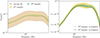 |
Fig. 1. Impact of sample variance and reweighting on the ΩGW spectrum. Left: 95% confidence on the spectrum calculated using 105 (106) samples in yellow (green) drawn from a fixed hyperparameter distribution, compared to the 95% confidence on the spectrum including uncertainty on the local merger rate parameter in brown. Unsurprisingly, the sample variance varies significantly with number of samples and when using large sample numbers is subdominant compared to population parameter uncertainty. Right: sample variance from the left panel compared to reweighted estimates of the ΩGW spectrum. The reweighted spectra lie neatly within the sample variance uncertainty bounds, implying that the reweighted spectrum is indistinguishable from a regularly sampled spectrum, with these sample numbers. |
4.1. Reweighting methodology
We lay out a simple method to efficiently calculate  for different sets of hyperparameters Λi describing the (detector frame) target population distributions, pd(Θ|Λi). The integral of (5) above allows the implementation of an importance sampling approach or reweighting,6 whereby
 (10)
(10)
where pd(Θ|Λ0) is chosen as the fiducial distribution, and w0 → 1 is the weight required to ‘transform’ between the fiducial distribution and the target distribution, relative to Λ1:
 (11)
(11)
In practice, this reweighting approach is more efficient than direct Monte Carlo integration when pd(Θ|Λ1) is hard to sample from but easy to evaluate. Therefore, we first draw a large set of samples θ from the fiducial population Λ0 and compute the probability of drawing those samples pd(Θ|Λ0). This is stored as the denominator in the weights w. Each time the integral of Eq. (10) is evaluated for some different population Λ1, it is only necessary to evaluate the probability of those fiducial samples under the target population pd(Θ|Λ1), as w is the only term that depends on Λ1. See also Appendix D of Turbang et al. (2024) for an analogous reweighting approach for the background spectrum calculation. The authors’ approach is technically equivalent; however, they choose to reweight the approximated event energy spectra calculated using Ajith et al. (2011), as opposed to the frequency domain 𝒫d quantity calculated from the event waveform.
The reweighting operation is directly implemented in the Monte Carlo evaluation described above, which is valid as long as a sufficient number of samples Θj are used:
 (12)
(12)
This allows us to evaluate the (costly) 𝒫d spectra only once, and reweight the contribution of each wave according to a desired target distribution.
In practice, we rely on the source-frame population distributions to sample the GW parameters. To convert these to detector frame, we evaluate the relevant Jacobian matrix assuming a fixed cosmology,
 (13)
(13)
4.2. Effective sample size and sample variance
As a check of the performance of our reweighting approach, we estimate the effective sample size Neff for different number of samples Ns and different ΩGW spectra, and ensure Neff ≫ 1. The effective sample size is calculated from the weights as Neff = Σw2/(Σw)2. We find, for a fixed reweighting set of Λ hyperparameters, that Neff ≈ 2 × 10⁴ for Ns = 5 × 10⁴, Neff ≈ 4 × 10⁴ for Ns = 105, and Neff ≈ 3 × 10⁵ for Ns = 106. In practice, these numbers depend on the size of the parameter space probed by the reweighting. In all implementations shown in this paper we use Ns = 1 × 10⁶ unless otherwise stated, and we have checked that the order of magnitude of Neff reported here remains reliable for all results shown.
The ΩGW spectrum is by definition a stochastic observable, and thus presents an intrinsic sample variance7. In particular,  is dominated by a Poisson process given the low merger rate of black hole binaries. We estimate the intrinsic variance of
  associated with different number of samples (which can be directly converted to different observation times, assuming a total merger rate) by calculating the spectrum using different sample draws from a fixed set of population priors. These are shown in Fig. 1 (left panel) using 105 and 106 samples, where the shading indicates the 95% interval over 1000 sets. In this case, increasing the number of samples by a factor of 10 decreases the width of the 95% interval by 52% on average, for frequencies between 20 and 500 Hz. This specific example corresponds to the following set of hyperparameters for the PLPP mass model: α = 3.5, β = 1, δm = 4.5, λ = 0.04, mmax = 100, mmin = 4, mpp = 34, σpp = 4. The redshift model is fixed to the default MD model defined above with a local merger rate of R0 = 15 Gpc−3 yr−1. In Fig. 1 we further compare these sample variance uncertainty bands to the 95% confidence on the spectrum including uncertainty on the local merger rate R0, drawn from Abbott et al. (2023a). Unsurprisingly, when using these large sample numbers, the sample variance is subdominant compared to population parameter uncertainty.
We compare this intrinsic uncertainty to reweighting. As can be seen in Fig. 1 (right panel), reweighted curves for  for the given set of Λ hyperparameters lie within the 95% sample uncertainty on the spectrum, for different values of Ns. This implies the reweighted
  spectrum for a given population model is within the intrinsic error on that spectrum, and is thus a fair approximation to make.
As we focus on BBHs in this paper, we drop the BBH subscript from  in what follows. We refer to the BBH spectrum unless otherwise specified.
5. Background projections using popstock
We studied the dependence of the amplitude, spectral shape, and uncertainty of ΩGW on various models and data products. These studies will fundamentally inform compact binary population parameter estimation campaigns with upcoming GW datasets, for example in the style of Callister et al. (2020) and Abbott et al. (2021c), which use constraints on (or, in the future, measurements of) the ΩGW spectrum.
We considered here a frequency range of 10 − 2000 Hz as this corresponds to the sensitivity of second-generation ground-based GW detectors, such as the current configurations of the LIGO, Virgo, and KAGRA instruments as well as their near-future improvements.
5.1. Mass and redshift models
With popstock we were able to rapidly assess the impact of different mass and redshift models on the projected ΩGW. Here we compared the PLPP and BPL mass models, and the UICV and MD redshift models, all introduced in Sect. 3. When comparing mass models, we fixed the mass model hyperparameters, while including the uncertainty on the local merger rate R0 from Abbott et al. (2023a) 8 assuming the MD redshift evolution with all other parameters fixed to the values discussed above. When comparing redshift models, we instead fixed the redshift model hyperparameters, while including the uncertainty from Abbott et al. (2023a) on the PLPP mass model. We deliberately chose values for certain Λ hyperparameters that are unrealistic and not favoured by the current data to showcase the effect different mass and redshift models may have on the ΩGW spectral shape.
A comparison between the PLPP and BPL mass models is shown in Fig. 2. The PLPP parameters are fixed to the same set used in Sect. 4.2, and BPL to α1 = −2, α2 = −1.4, β = 1, b = 0.4 (see Sect. 3 for details on the parameters). As PLPP is commonly used as a mass model when generating ΩGW forecasts (as in Abbott et al. 2021c, 2023a), we took this as the fiducial model to produce ΩGW spectra and compared those obtained with the BPL mass model against these. We note that in particular the choice of α2 > α1 for BPL here implies a larger amount of high-mass binaries in the distribution, as seen in the left panel of Fig. 2, where the primary mass probability distributions are shown. These more massive binaries merge at lower frequencies and their emission is further redshifted into the lower end of the frequency range considered here. We recall that, for example, we detect an equal-mass binary with true component masses of 70 M⊙ merging around ∼60 Hz at z = 0 and ∼30 Hz at z = 1 (see e.g. Renzini et al. 2024 for more considerations along this line). As seen in the right panel of Fig. 2, this both boosts the amplitude of ΩGW at all frequencies below a few hundred Hz, and changes the spectral shape at these frequencies, when compared to the PLPP mass spectrum. Specifically, the typical turnover in the spectrum corresponding to the frequency at which most binaries have merged is broken into two turnovers: one for the higher mass binaries (below 100 Hz) and one for the lower mass ones (around 300 Hz). This effect is certainly fuelled by the unrealistic parameter choice made for BPL (α2 > α1). Comparatively, the PLPP model gives rise to a single turnover with a plateau between ∼100 and 400 Hz, which presents small features (‘wiggles’), which are related to the redshifting of the peak at 33 M⊙. Futhermore, the spectral index at lower frequencies is more peaked than that of the PLPP model. A simple broken-power-law fit to the two sets of curves shown in the right panel of Fig. 2 yields α = 0.61 and α = 0.76 for the lower frequency region of the ΩGW spectrum corresponding to the PLPP and BPL mass models, respectively. A broader discussion on data-informed spectral indices is postponed to Sect. 5.3.
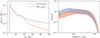 |
Fig. 2. Impact of the primary mass distribution on the ΩGW spectrum. The left panel shows the two primary mass model probability densities used throughout. The right panel shows the 95% confidence intervals for ΩGW using the two mass models, including uncertainty on the local merger rate from Abbott et al. (2023a). |
The uncertainty on the local rate R0 implies that there is significant overlap between the 95% credible envelope of the spectrum from these two mass models, suggesting it would be challenging to distinguish mass spectrum features from redshift ones from a measurement of ΩGW alone. The overlap would be even greater when including the full uncertainty on the redshift model parameters. However, if a large amplitude and large spectral index (i.e. α > 2/3) ΩGW is observed at low frequencies, we expect a mass model that admits high mass binaries (such as the BPL one showed here) to be favoured.
In Fig. 3 we compare the effect of the UICV and MD redshift models on ΩGW. We fix the local merger rate to R0 = 15 Gpc−3 yr−1, and compare a UICV rate evolution to the default MD evolution (see Sect. 3), while we include the uncertainty on the PLPP mass model from Abbott et al. (2023a). Most notably, the UICV model impacts the overall amplitude of the ΩGW spectrum across all frequencies. In this test case, the decrease in amplitude when assuming UICV is approximately constant (and equal to a factor of ∼4) between 10 and 100 Hz, and is due to the lower merger rate between 1 < z < 4. This effect is much greater than the impact of the uncertainty on the mass model, confirming that a measurement of ΩGW provides significant information on the merger rate redshift evolution (as also seen in Callister et al. 2016, 2020; Renzini et al. 2024). The turnover in the spectrum appears shifted to slightly higher frequencies in UICV, possibly due to the slightly higher rate fraction at low redshift compared to MD, which instead increases as a power law9. Otherwise, the different redshift models do not appear to cause large variations in the overall shape of the spectrum, suggesting that the mass spectrum dominates these features.
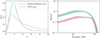 |
Fig. 3. Impact of the merger rate redshift distribution model on the ΩGW spectrum. The left panel shows the two redshift evolution model probability densities used throughout. The right panel shows the 95% confidence intervals for ΩGW using the two merger rate models, including uncertainty on the PLPP mass model from Abbott et al. (2023a), as described in Sect. 3. |
A natural extension of this study is to consider BBH mass spectra that evolve with redshift. This will mix the effects seen here when considering independent contributions, and in principle will need to be appropriately included in parameter estimation studies to avoid biases.
5.2. Waveform approximants
The choice of waveform approximant, while central in certain studies of individual compact binary merger events, has been explored very little in the context of the compact binary background signal. In previous work (see e.g. the approximations made in Meacher et al. 2015; Callister et al. 2016; Mukherjee & Silk 2021), it was deemed sufficient to capture solely the evolution of the GW amplitude as a function of frequency as the background ΩGW contains no phase information. This evolution can be tracked analytically up to arbitrary post-Newtonian (PN) order, considerably speeding up the calculation of ΩGW compared to calculating full waveforms for large sets of events. Specifically, most works employ the amplitude component of frequency-domain inspiral-merger-ringdown (IMR) waveforms (Ajith et al. 2008, 2011) defined analytically by parts, where the transition of the GW from one phase to the next is set by the specific intrinsic parameters of the binary (mass and spin). As the background has remained a weak signal in the current LVK data, a precise quantification of the systematic differences between background estimates with different waveform approximants has not been necessary. However, as detector sensitivities improve and detection becomes a real possibility, all modelling systematics are important to quantify (see also Zhou et al. 2023; Song et al. 2024). Here, we investigated the effect of the waveform approximant using popstock and confirmed whether it is subdominant to the impact of population uncertainties.
We focus here on the IMRPhenom family of waveforms commonly used in the literature to compute ΩGW, as well as an effective-one-body (EOB) numerical-relativity (NR) waveform model. In all cases, we omitted spin effects, setting both black hole spins to 0. The following specific waveforms were used:
-
IMRPhenomA (Ajith et al. 2008): The first IMR waveform, developed for GW data analysis in the frequency domain for non-spinning binaries. Here the amplitude is expanded to leading post-Newtonian (0-PN) order, implying that the inspiral phase presents the characteristic f2/3 trend (in ΩGW units).
-
IMRPhenomB (Ajith et al. 2011): A direct successor to IMRPhenomA, this waveform includes higher order corrections in the amplitude term up to 1.5-PN and includes non-zero aligned spin. These correct the spectral shape of the waveform amplitude, as a function of both mass and spin.
-
IMRPhenomD (Khan et al. 2016): A recent waveform including corrections up to 3-PN order in the amplitude and a more sophisticated fit to numerical relativity compared to IMRPhenomA and B.
-
SEOBNRv2 (Pürrer 2016): An EOB NR waveform for spin-aligned BBHs, calculated numerically in the frequency domain.
A comparison between the ΩGW spectra calculated for the same BBH population using the waveforms above is presented in Fig. 4. We show the 95% confidence contours on the population ΩGW including the uncertainty on the mass model (PLPP) and the local merger rate R0 assuming a fixed MD redshift evolution (as defined above).
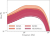 |
Fig. 4. Impact of the waveform model on the ΩGW spectrum. The shading indicates the 95% confidence on the spectrum including the uncertainty on the PLPP mass model and the local merger rate, assuming a fixed MD redshift evolution. |
We find that when employing the 0-PN IMRPhenomA waveform, the background signal is overestimated at all frequencies by up to 50% in the range 10 < f < 1000 Hz compared to IMRPhenomB; this is due to the missing amplitude corrections to the inspiral phase (see e.g. the differences in Eq. (4.13) of Ajith et al. 2008 and Eq. (1) of Ajith et al. 2011). While the amplitude estimates for IMRPhenomA and B agree at f ≡ 0, they diverge for f > 0 as the amplitude evolution with frequency is ΩA ∝ f2/3 for IMRPhenomA and ΩB ∝ fα < 2/3 for IMRPhenomB. The trend of α depends on the specific mass, redshift, and spin realisation, as discussed in Sect. 5.1. This result shows that the somewhat basic assumption that the compact binary background at frequencies under ∼100 Hz is well-approximated by a two-thirds power law can be upgraded and informed by likely population models to optimise background searches.
Differences due to the use of IMRphenomB/D and SEOBNRv2 approximants are comparable to each other and would be hard to distinguish from population uncertainties. Nevertheless, we comment that the different NR calibration used in IMRphenomD compared to B is evident in the impact due to the inspiral phase on the GWB signal, as the frequency evolution at low frequency is slightly modified, and SEOBNRv2 estimates an overall lower background than the IMRPhenom waveforms.
The impact of including higher-order modes in the waveform calculation on the background spectrum was found to be negligible; a comparison between spectra calculated with the IMRPhenomD and IMRPhenomXPHM waveforms is included for completeness in Appendix B.
5.3. O3 population samples
We conclude our analyses by combining the uncertainties on the mass and redshift distributions drawn directly from the LVK GWTC-3 population analysis (Abbott et al. 2023a). We limit our focus to the MD redshift model for BBHs as this is the only model we have viable posterior samples for. In the case of the low-redshift merger rate parameters (R0, γ), we used the samples from the power-law redshift inference results released in LIGO Scientific Collaboration, Virgo Collaboration, KAGRA Collaboration (2021) for the power-law redshift model, while when including high-redshift features (zmax, κ) we used the results obtained performing inference on the entire MD model, as done in Abbott et al. (2021c).
The results obtained progressively varying the redshift hyperparameters are shown in Fig. 5 (left panel). We included uncertainty over the entire PLPP mass hyperparameter space, while varying the following:
 |
Fig. 5. Uncertainty on the expected ΩGW spectrum from BBHs due to uncertainty on the merger rate evolution parameters. Left: 95% confidence levels on the projected ΩGW spectrum including uncertainty on the PLPP mass model and assuming a MD merger rate model with different levels of uncertainty. The hatched outline reports previous results published in Abbott et al. (2023a). Right: zoomed-in comparison at low frequencies of the uncertainty on the ΩGW spectrum when varying R0 vs. R0 and γ, reporting average spectral indices referred to these two contours. |
-
(i)
just the local merger rate R0, assuming a fixed broken-power-law merger rate evolution with parameters fixed to those discussed in Sect. 3;
-
(ii)
both R0 and the local power-law index γ, keeping the high-redshift parameters fixed;
-
(iii)
all parameters for the merger rate, including the turnover redshift zpeak and high-redshift power-law index κ.
In cases (i) and (ii) the samples were drawn from the power-law redshift model posteriors of Abbott et al. (2023a). In case (iii), the samples were instead drawn from a full GWTC-3, O1–O2–O3 joint stochastic-population analysis (similar to Abbott et al. 2021c; for details on how this analysis was carried out, see Callister et al. 2020) as these also include posteriors on the higher redshift evolution of R(z) (Callister 2024).
We compared the 95% confidence levels on ΩGW in case (i) with published results (shown in Fig. 5 in hatched outline10) and find them to be consistent. We note that the corresponding LVK contours draw from the same PLPP mass posterior and local merger rate posterior, but assume a different redshift evolution (see the original paper discussion Abbott et al. 2023a), which explains the small differences between the curves at low frequency and the different turnover trend at high frequency, which is dominated by low-redshift effects. Specifically, the redshift model used sampled a time-delay distribution between binary formation and merger, where the binary formation rate was fixed to follow the star formation rate of Vangioni et al. (2015), and the time-delay distribution was in the shape of  . This model cannot be well approximated with a simple broken power law. The LVK contour was calculated assuming the IMRPhenomB analytic waveform model. Case (ii) and case (iii) give almost identical contours, which implies that the population analysis Abbott et al. (2023a) and the stochastic constraints Abbott et al. (2021c) carry little information about the high-redshift evolution of the merger rate. Furthermore, they show that the uncertainty on the local merger rate evolution alone could account for an increase of up to a factor of ∼5 in the ΩGW spectrum. This could have considerable consequences on the detectability of the signal. In the right panel of Fig. 5 we show a zoomed-in image of the [20, 200] Hz portion of the spectra in cases (i) and (ii), and provide results of single power-law fits to the envelope of ΩGW curves. The average α spectral indices found are consistent with each other: α(i) = 0.59 ± 0.02 for (i), and α(ii) = 0.60 ± 0.03 for (ii). This confirms that γ has no impact on the low-frequency spectral shape of ΩGW, but only on its amplitude.
We repeated the ΩGW calculation varying R0 and γ using the BPL mass model, sampling over the joint mass and redshift posteriors obtained by performing population inference on the GWTC-3 catalogue (samples are publicly available as a part of the example sample sets in the popstock package repository). We compared these results with the PLPP results described above in Fig. 6, overlaying the 2σ LVK power-law-integrated sensitivity curves (Thrane & Romano 2013) already shown in Abbott et al. (2023a). These track the present and future upgrades to the LIGO and Virgo facilities, where ‘O3 sensitivity’ is given by the O3 measured spectra, ‘Design HLV’ is produced assuming projections shown in Abbott et al. (2018) and is expected to approximate the sensitivity at the end of the O4 observing run (currently ongoing), and ‘Design A+’ refers to the sensitivity projected for the next observing run O5 assuming one year of continuous data and all planned improvements to the detectors are implemented and successful.
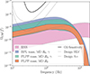 |
Fig. 6. Projections of the background ΩGW spectrum, given our knowledge of the compact binary population. The shaded regions outline 90% credible bands for the GWB from BBHs and BNS (in pink), including the uncertainty on the mass and redshift models for these sources using the samples released in Abbott et al. (2023a), LIGO Scientific Collaboration, Virgo Collaboration, KAGRA Collaboration (2021). For BBHs we report the uncertainty due to two mass models: the PLPP mass model, assuming a MD redshift model with uncertain local merger rate R0 (orange), and also uncertain low-redshift power-law index γ (green); and the BPL mass model, assuming a MD redshift model with uncertain R0 and γ. Current and projected sensitivity curves are included for reference. |
The BPL mass model predicts a systematically larger background, by a factor of 1.4 on average, which hints at the possibility of a louder signal than previously projected, and thus the prospect of a detection of the stochastic signal before reaching the Design A+ LIGO-Virgo sensitivity. For completeness, we also include the expected background signal arising from binary neutron stars (BNS) in Fig. 6. This signal is strongly dominated by uncertainties given the very few detections of BNS mergers (Abbott et al. 2017, 2020). The projection is calculated employing the NRTidalv2 model discussed in Dietrich et al. (2019). We assume a uniform mass model between 1 and 2.5 M⊙, as in Abbott et al. (2023a), and a merger rate model corresponding to a time-delayed SFR as used for projections presented in Abbott et al. (2021c)
11. We draw the local merger rate R0 from the corresponding posterior samples presented in Abbott et al. (2023a), LIGO Scientific Collaboration, Virgo Collaboration, KAGRA Collaboration (2021); for reference, we refer to the samples that set the  Gpc−3 yr−1 upper limit.
6. Conclusions
We present a novel method and code-base for rapid calculations of the background spectrum of inspiralling and coalescing compact binaries, starting from a given population model and hyperparameter sets.
We quantified the joint uncertainty on the ΩGW spectrum from both the mass and redshift distributions of the BBH population, given the most recent results from the LVK collaboration. Predictably, the uncertainty on the local merger rate and its evolution (together with the uncertainty on the mass model) dominated the expected amplitude of the spectrum, and can have significant implications on detectability.
Furthermore, we find that for the preferred mass model (power-law-plus-peak), the low-frequency spectral index of the stochastic background signal is α = 0.6. Previous detection approaches assumed α = 2/3 (for example Abbott et al. 2021b,c; Renzini & Contaldi 2019); this result was based on the waveform used to calculate the expected GWB and its PN order expansion, as first seen in Phinney (2001) and then Sesana et al. (2008). We find that, when employing 0-PN order waveforms, there is a tension between projections for ΩGW from the presently observed population which competes with population uncertainty itself. The mismatch between the treatment of the late inspiral phase in IMR waveforms is particularly significant as it is present throughout the entire ΩGW spectrum and in particular at lower frequencies, where current detector sensitivities peak.
Differences between the specific background realisations and the number of samples also produce different projections that may give rise to small tensions in the higher frequency range, where the spectra present a turnover that is highly dependent on the binary mass distribution and local features of the merger rate. Current-generation detectors are not sensitive to this region of the spectrum; however, this will have significant implications for next-generation interferometers.
In conclusion, the specific population properties of the coalescing compact binary population as well as the specific realisation during our observations will play a role in detection capabilities. In particular, within current binary black hole population uncertainties, a low-redshift amplification of the merger rate and a larger population of higher-mass binaries contribute to a significant boost in the background amplitude, in the LVK sensitivity band, which could lead to early detection. On the other hand, more astrophysically motivated BBH rate evolution models relate the merger rate to binary progenitor features, and reparametrise the merger rate density in terms of, for example, the time-to-merger delay distribution and the host galaxy metallicity (Fishbach & Kalogera 2021; Chruślińska 2024). These models have recently been employed in joint analyses of the GWTC-3 catalogue and LVK stochastic upper limits (Turbang et al. 2024), and may provide alternative forecasts of the uncertainty on the ΩGW spectrum, as we gather more GW data. These models will progressively be included and updated in popstock. With popstock, we provide the GW community engaged in GW source modelling, data analysis, and astrophysical interpretation with a user-friendly tool for rapid background spectrum evaluation and easy integration of new models as our understanding of the GW universe expands.
For discussions on residual backgrounds, in particular in the context of next-generation ground-based interferometers, we refer to Sachdev et al. (2020), Zhou et al. (2023), and Bellie et al. (2024), among others.
In the case of a stochastic signal described as a superposition of plane waves, as is often the case for cosmological signals, the signal can be thought of as a wave where the Fourier amplitudes are stochastic fields, the parameters Θ describe the field, and the power is the second-order moment of the field (Renzini et al. 2022).
This feature is found in the data, but recent works have cast doubt on whether it can be attributed to the pulsational pair instability mechanism (Golomb et al. 2023; Hendriks et al. 2023).
Reweighting has become a popular tool for efficient Monte Carlo computations in GW astronomy; see e.g. Talbot et al. (2019), Payne et al. (2019), Hourihane et al. (2023), Talbot & Golomb (2023) for a review of some applictions of this method in the GW field.
See Lamb & Taylor (2024) for an analytic study of the massive black hole background spectral variance, in the case of a signal in the pulsar timing array detection band.
Specifically, we employed samples from the posterior fit of the power-law redshift model; as in Abbott et al. (2023a), no broken-power-law redshift model was used.
This is evident in the area in the left panel of Fig. 3, where the UICV model p(z) lies above the MD p(z) at z < 1.
The hatched outline is exactly the green region highlighted in Fig. 23 of Abbott et al. (2023a), which is publicly available in LIGO Scientific Collaboration, Virgo Collaboration, KAGRA Collaboration (2021).
This model assumes that the BNS progenitor formation rate is proportional to the SFR, and that the distribution of time delays between binary formation and merger is inversely proportional to the time delays distributed between 20 Myr and 13.5 Gyr.
Acknowledgments
We thank Patrick Meyers and Alan Weinstein for invaluable discussions and insight. We thank Thomas Callister for providing the population samples in Callister (2024), and for carefully reading our work. We thank Nicholas Loutrel for consulting on waveform models and their features. AIR is supported by the European Union’s Horizon 2020 research and innovation programme under the Marie Sklodowska-Curie grant agreement No 101064542, and acknowledges support from the NSF award PHY-1912594. JG is supported by NSF award No. 2207758. The authors are grateful for computational resources provided by the LIGO Laboratory and supported by National Science Foundation Grants PHY-0757058 and PHY-0823459. This material is based upon work supported by NSF’s LIGO Laboratory which is a major facility fully funded by the National Science Foundation.
References
- Aasi, J., Abbott, B. P., Abbott, R., et al. 2015, Class. Quant. Grav., 32, 074001 [Google Scholar]
- Abbott, B. P., Abbott, R., Abbott, T. D., et al. 2017, Phys. Rev. Lett., 119, 161101 [Google Scholar]
- Abbott, B. P., Abbott, R., Abbott, T. D., et al. 2018, Liv. Rev. Rel., 21, 3 [Google Scholar]
- Abbott, B. P., Abbott, R., Abbott, T. D., et al. 2020, ApJ, 892, L3 [NASA ADS] [CrossRef] [Google Scholar]
- Abbott, R., Abbott, T. D., Abraham, S., et al. 2021a, ApJ, 913, L7 [NASA ADS] [CrossRef] [Google Scholar]
- Abbott, R., Abbott, T. D., Abraham, S., et al. 2021b, Phys. Rev. D, 104, 022005 [NASA ADS] [CrossRef] [Google Scholar]
- Abbott, R., Abbott, T. D., Abraham, S., et al. 2021c, Phys. Rev. D, 104, 022004 [NASA ADS] [CrossRef] [Google Scholar]
- Abbott, R., Abbott, T. D., Acernese, F., et al. 2023a, Phys. Rev. X, 13, 011048 [NASA ADS] [Google Scholar]
- Abbott, R., Abbott, T. D., Acernese, F., et al. 2023b, Phys. Rev. X, 13, 041039 [Google Scholar]
- Acernese, F., Agathos, M., Agatsuma, K., et al. 2015, Class. Quant. Grav., 32, 024001 [Google Scholar]
- Ajith, P., Babak, S., Chen, Y., et al. 2008, Phys. Rev. D, 77, 104017, Erratum: 2009, Phys. Rev. D, 79, 129901 [NASA ADS] [CrossRef] [Google Scholar]
- Ajith, P., Hannam, M., Husa, S., et al. 2011, Phys. Rev. Lett., 106, 241101 [NASA ADS] [CrossRef] [Google Scholar]
- Akutsu, T., Ando, M., Arai, K., et al. 2019, Nat. Astron., 3, 35 [NASA ADS] [CrossRef] [Google Scholar]
- Ashton, G., Húbner, M., Lasky, P. D., et al. 2019, ApJS, 241, 27 [NASA ADS] [CrossRef] [Google Scholar]
- Price-Whelan, A. M. 2022, ApJ, 935, 167 [NASA ADS] [CrossRef] [Google Scholar]
- Belczynski, K., Holz, D. E., Bulik, T., & O’Shaughnessy, R. 2016, Nature, 534, 512 [NASA ADS] [CrossRef] [Google Scholar]
- Bellie, D. S., Banagiri, S., Doctor, Z., & Kalogera, V. 2024, Phys. Rev. D, 110, 023006 [NASA ADS] [CrossRef] [Google Scholar]
- Callister, T. 2024, Binary Black Hole Merger Rate Constraints Using GWTC-3 and Full-O3 Stochastic Background Constraints [Google Scholar]
- Callister, T. A., & Farr, W. M. 2024, Phys. Rev. X, 14, 021005 [NASA ADS] [Google Scholar]
- Callister, T., Sammut, L., Qiu, S., Mandel, I., & Thrane, E. 2016, Phys. Rev. X, 6, 031018 [NASA ADS] [Google Scholar]
- Callister, T., Fishbach, M., Holz, D., & Farr, W. 2020, ApJ, 896, L32 [NASA ADS] [CrossRef] [Google Scholar]
- Carroll, S. M. 2004, Spacetime and Geometry. An Introduction to General Relativity (Cambridge: Cambridge University Press) [Google Scholar]
- Chruślińska, M. 2024, Ann. Phys., 536, 2200170 [CrossRef] [Google Scholar]
- Dietrich, T., Samajdar, A., Khan, S., et al. 2019, Phys. Rev. D, 100, 044003 [NASA ADS] [CrossRef] [Google Scholar]
- Dominik, M., Berti, E., O’Shaughnessy, R., et al. 2015, ApJ, 806, 263 [Google Scholar]
- Fishbach, M., & Kalogera, V. 2021, ApJ, 914, L30 [CrossRef] [Google Scholar]
- Fishbach, M., Holz, D. E., & Farr, W. M. 2018, ApJ, 863, L41 [NASA ADS] [CrossRef] [Google Scholar]
- Golomb, J., Isi, M., & Farr, W. 2023, ArXiv e-prints [arXiv:2312.03973] [Google Scholar]
- Harris, C. R., Millman, K. J., van der Walt, S. J., et al. 2020, Nature, 585, 357 [NASA ADS] [CrossRef] [Google Scholar]
- Hendriks, D. D., van Son, L. A. C., Renzo, M., Izzard, R. G., & Farmer, R. 2023, MNRAS, 526, 4130 [NASA ADS] [CrossRef] [Google Scholar]
- Hourihane, S., Meyers, P., Johnson, A., Chatziioannou, K., & Vallisneri, M. 2023, Phys. Rev. D, 107, 084045 [NASA ADS] [CrossRef] [Google Scholar]
- Isaacson, R. A. 1968, Phys. Rev., 166, 1272 [NASA ADS] [CrossRef] [Google Scholar]
- Khan, S., Husa, S., Hannam, M., et al. 2016, Phys. Rev. D, 93, 044007 [Google Scholar]
- Lamb, W. G., & Taylor, S. R. 2024, ApJ, 971, L10 [NASA ADS] [CrossRef] [Google Scholar]
- LIGO Scientific Collaboration 2020, Astrophysics Source Code Library [record ascl:2012.021] [Google Scholar]
- LIGO Scientific Collaboration, Virgo Collaboration, KAGRA Collaboration (Abbott, R., et al.) 2021, GWTC-3: Compact Binary Coalescences Observed by LIGO and Virgo During the Second Part of the Third Observing Run - Parameter estimation data release [Google Scholar]
- London, L., Khan, S., Fauchon-Jones, E., et al. 2018, Phys. Rev. Lett., 120, 161102 [NASA ADS] [CrossRef] [Google Scholar]
- Madau, P., & Dickinson, M. 2014, ARA&A, 52, 415 [Google Scholar]
- Maggiore, M. 2007, Gravitational Waves. Vol. 1: Theory andExperiments (Oxford: Oxford University Press) [CrossRef] [Google Scholar]
- Mandel, I., & de Mink, S. E. 2016, MNRAS, 458, 2634 [NASA ADS] [CrossRef] [Google Scholar]
- Meacher, D., Thrane, E., & Regimbau, T. 2014, Phys. Rev. D, 89, 084063 [NASA ADS] [CrossRef] [Google Scholar]
- Meacher, D., Coughlin, M., Morris, S., et al. 2015, Phys. Rev. D, 92, 063002 [NASA ADS] [CrossRef] [Google Scholar]
- Mukherjee, S., & Silk, J. 2021, MNRAS, 506, 3977 [NASA ADS] [CrossRef] [Google Scholar]
- Payne, E., Talbot, C., & Thrane, E. 2019, Phys. Rev. D, 100, 123017 [NASA ADS] [CrossRef] [Google Scholar]
- Phinney, E. S. 2001, ArXiv e-prints [arXiv:astroph/0108028] [Google Scholar]
- Pratten, G., García-Quirós, C., Marta Colleoni, M., et al. 2021, Phys. Rev. D, 103, 104056 [NASA ADS] [CrossRef] [Google Scholar]
- Pürrer, M. 2016, Phys. Rev. D, 93, 064041 [CrossRef] [Google Scholar]
- Regimbau, T. 2007, Phys. Rev. D, 75, 043002 [NASA ADS] [CrossRef] [Google Scholar]
- Regimbau, T. 2011, Res. Astron. Astrophys., 11, 369 [CrossRef] [Google Scholar]
- Regimbau, T. 2022, Symmetry, 14 [Google Scholar]
- Renzini, A., & Contaldi, C. 2019, Phys. Rev. D, 100, 063527 [NASA ADS] [CrossRef] [Google Scholar]
- Renzini, A. I., Goncharov, B., Jenkins, A. C., & Meyers, P. M. 2022, Galaxies, 10, 34 [NASA ADS] [CrossRef] [Google Scholar]
- Renzini, A. I., Callister, T. A., Chatziioannou, K., & Farr, W. M. 2024, Phys. Rev., 110, 023014 [NASA ADS] [Google Scholar]
- Rodriguez, C. L., Amaro-Seoane, P., Chatterjee, S., & Rasio, F. A. 2018, Phys. Rev. Lett., 120, 151101 [NASA ADS] [CrossRef] [Google Scholar]
- Sachdev, S., Regimbau, T., & Sathyaprakash, B. S. 2020, Phys. Rev. D, 102, 024051 [NASA ADS] [CrossRef] [Google Scholar]
- Saffer, A., Yunes, N., & Yagi, K. 2018, Class. Quant. Grav., 35, 055011 [NASA ADS] [CrossRef] [Google Scholar]
- Sah, M. R., & Mukherjee, S. 2023, MNRAS, 527, 4100 [CrossRef] [Google Scholar]
- Sesana, A., Vecchio, A., & Colacino, C. N. 2008, MNRAS, 390, 192 [NASA ADS] [CrossRef] [Google Scholar]
- Song, H., Liang, D., Wang, Z., & Shao, L. 2024, Phys. Rev. D, 109, 123014 [NASA ADS] [CrossRef] [Google Scholar]
- Talbot, C., & Golomb, J. 2023, MNRAS, 526, 3495 [NASA ADS] [CrossRef] [Google Scholar]
- Talbot, C., & Thrane, E. 2018, ApJ, 856, 173 [NASA ADS] [CrossRef] [Google Scholar]
- Talbot, C., Smith, R., Thrane, E., & Poole, G. B. 2019, Phys. Rev. D, 100, 043030 [NASA ADS] [CrossRef] [Google Scholar]
- Thrane, E., & Romano, J. D. 2013, Phys. Rev. D, 88, 124032 [NASA ADS] [CrossRef] [Google Scholar]
- Turbang, K., Lalleman, M., Callister, T. A., & van Remortel, N. 2024, ApJ, 967, 142 [NASA ADS] [CrossRef] [Google Scholar]
- Vangioni, E., Olive, K. A., Prestegard, T., et al. 2015, MNRAS, 447, 2575 [Google Scholar]
- Virtanen, P., Gommers, R., Oliphant, T. E., et al. 2020, Nat. Methods, 17, 261 [Google Scholar]
- Wu, C., Mandic, V., & Regimbau, T. 2012, Phys. Rev. D, 85, 104024 [NASA ADS] [CrossRef] [Google Scholar]
- Zhou, B., Reali, L., Berti, E., et al. 2023, Phys. Rev. D, 108, 064040 [NASA ADS] [CrossRef] [Google Scholar]
- Zhu, X.-J., Howell, E., Regimbau, T., Blair, D., & Zhu, Z.-H. 2011, ApJ, 739, 86 [NASA ADS] [CrossRef] [Google Scholar]
Appendix A: Deriving the energy in GWs
We derive here the energy spectrum dE/df carried by gravitational waves, in vacuum (see e.g. Maggiore 2007; Saffer et al. 2018; Carroll 2004). We start by expanding the perturbed metric gμν to second order,
 (A.1)
(A.1)
where ημν is the Minkowski flat metric and it is assumed that the perturbation  is ith order in some small parameter controlling the scale of hμν. Substituting the above into the Einstein field equation gives
![Mathematical equation: $$ \begin{aligned} G_{\mu \nu }\left[h^{(1)}\right] + G_{\mu \nu }\left[\left(h^{(1)}\right)^2\right] + G_{\mu \nu }\left[h^{(2)}\right]= 8 \pi G \tau _{\mu \nu }\,, \end{aligned} $$](/articles/aa/full_html/2024/11/aa51374-24/aa51374-24-eq34.gif) (A.2)
(A.2)
Where the first term is the Einstein tensor linear in the first order perturbation, the second is the Einstein tensor terms quadratic in the first order perturbation, and the third term is linear in the second-order perturbation. In vacuum, τμν = 0, and the solution for h(1) (i.e. the plane wave solution) reduces the first term to ![Mathematical equation: $ G_{\mu \nu}\left[h^{(1)}\right] = \Box h^{(1)}_{\mu \nu} = 0 $](/articles/aa/full_html/2024/11/aa51374-24/aa51374-24-eq35.gif) , in the Lorenz gauge. We can therefore rearrange the above into a form that resembles the Einstein field equation,
, in the Lorenz gauge. We can therefore rearrange the above into a form that resembles the Einstein field equation,
![Mathematical equation: $$ \begin{aligned} G_{\mu \nu }\left[h^{(2)}\right] = -G_{\mu \nu }\left[\left(h^{(1)}\right)^2\right], \end{aligned} $$](/articles/aa/full_html/2024/11/aa51374-24/aa51374-24-eq36.gif) (A.3)
(A.3)
where the first-order term  squared effectively forms a stress-energy (RHS) that sources the second order curvature (LHS). In this analogy to the RHS of the Einstein equation, we can define the effective stress energy (pseudo)-tensor of GWs Isaacson (1968):
![Mathematical equation: $$ \begin{aligned} \tau _{\mu \nu } \equiv -\frac{1}{8\pi G} G_{\mu \nu }\left[\left(h^{(1)}\right)^2\right]. \end{aligned} $$](/articles/aa/full_html/2024/11/aa51374-24/aa51374-24-eq38.gif) (A.4)
(A.4)
A nice feature here is that the LHS of Eq. A.3 satisfies the contracted Bianchi identities and therefore the RHS is divergence-free and can be interpreted as conserving energy according to some observer. Expanding out (A.4) gives
 (A.5)
(A.5)
The conservation law ∂μtμν = 0 implies
 (A.6)
(A.6)
where τ00 can be interpreted as a volumetric energy density, such that the energy E is defined as E = ∫d3xτ00 and therefore the associated power is
 (A.7)
(A.7)
Substituting into Eq. A.6 yields
 (A.8)
(A.8)
which simplifies to
 (A.9)
(A.9)
for a wave moving along direction  . We employ the divergence theorem to convert the volume integral into a surface integral,
 (A.10)
which gives an expression for the energy flux (energy per unit time per unit area):
 (A.11)
as ∂0hij = −∂zhij = −∂0hij holds for a wave solution. Considering our gauge, the only surviving terms are those for μ, ν = 1 or 2,
 (A.12)
and substituting in the polarisation components of the wave hμν in the TT gauge yields
 (A.13)
Solving for the energy flux of gravitational waves of Eq. (A.10) gives
 (A.14)
where we have switched to the absolute value of this quantity with the understanding that GWs are removing energy from the system. The surface area energy density is then defined as
 (A.15)
To expand the above we recall that, for a plane wave,
 (A.16)
where in the final equivalence we have directly employed the definitaion of a Fourier transform. Recalling Parseval’s theorem, we can write the surface area energy density in terms of the Fourier transform  ,
,
 (A.17)
where the integral is taken over the sphere surrounding the source. Note that h+ and h× terms include dependence on inclination ι and reference phase ϕ0 (or, equivalently, the observer’s position along the azimuth) and therefore must be included in the integral over the area.
Appendix B: Impact of higher order modes on the GWB spectrum
For the sake of completeness, we append here findings on the impact on the ΩGW spectrum due to the inclusion of higher order modes in the waveform model. Higher order modes are subdominant harmonics excited during GW emission, where the dominant harmonic is the ℓ = 2, m = 2 mode London et al. (2018). We compare the 95% confidence bands shown in 5.2 for the IMRPhenomD waveform model with bands obtained using the IMRPhenomXPHM approximant Pratten et al. (2021), which includes the (ℓ, |m|) = (2, 2), (2, 1), (3, 3), (3, 2), (4, 4) modes. As may be seen in Fig. A.1, for the population of binaries considered in 5.2 which in particular is non-spinning and non-precessing, there are negligible differences between the use of IMRPhenomD and IMRPhenomXPHM. This is particularly evident when comparing the ΩGW spectrum calculated using the same event samples employing the two waveforms, shown as dashed and dotted curves in the left panel of Fig. A.1. The percent difference between these two curves is reported in the right panel of Fig. A.1, which remains consistently below 10% across the spectrum and is under 3% for frequencies below 100 Hz.
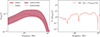 |
Fig. A.1. Impact of the inclusion of higher order modes in the waveform model employed to evaluate the ΩGW spectrum. On the left: 95% confidence on the spectrum including the uncertainty on the PLPP mass model and the local merger rate, assuming a fixed MD redshift evolution. On the right: percent difference %ΔΩGW(f) between ΩGW spectra calculated using the same event samples, shown as dashed and dotted curves on the left panel. |
All Tables
All Figures
|
Fig. 1. Impact of sample variance and reweighting on the ΩGW spectrum. Left: 95% confidence on the spectrum calculated using 105 (106) samples in yellow (green) drawn from a fixed hyperparameter distribution, compared to the 95% confidence on the spectrum including uncertainty on the local merger rate parameter in brown. Unsurprisingly, the sample variance varies significantly with number of samples and when using large sample numbers is subdominant compared to population parameter uncertainty. Right: sample variance from the left panel compared to reweighted estimates of the ΩGW spectrum. The reweighted spectra lie neatly within the sample variance uncertainty bounds, implying that the reweighted spectrum is indistinguishable from a regularly sampled spectrum, with these sample numbers. |
| In the text | |
|
Fig. 2. Impact of the primary mass distribution on the ΩGW spectrum. The left panel shows the two primary mass model probability densities used throughout. The right panel shows the 95% confidence intervals for ΩGW using the two mass models, including uncertainty on the local merger rate from Abbott et al. (2023a). |
| In the text | |
|
Fig. 3. Impact of the merger rate redshift distribution model on the ΩGW spectrum. The left panel shows the two redshift evolution model probability densities used throughout. The right panel shows the 95% confidence intervals for ΩGW using the two merger rate models, including uncertainty on the PLPP mass model from Abbott et al. (2023a), as described in Sect. 3. |
| In the text | |
|
Fig. 4. Impact of the waveform model on the ΩGW spectrum. The shading indicates the 95% confidence on the spectrum including the uncertainty on the PLPP mass model and the local merger rate, assuming a fixed MD redshift evolution. |
| In the text | |
|
Fig. 5. Uncertainty on the expected ΩGW spectrum from BBHs due to uncertainty on the merger rate evolution parameters. Left: 95% confidence levels on the projected ΩGW spectrum including uncertainty on the PLPP mass model and assuming a MD merger rate model with different levels of uncertainty. The hatched outline reports previous results published in Abbott et al. (2023a). Right: zoomed-in comparison at low frequencies of the uncertainty on the ΩGW spectrum when varying R0 vs. R0 and γ, reporting average spectral indices referred to these two contours. |
| In the text | |
|
Fig. 6. Projections of the background ΩGW spectrum, given our knowledge of the compact binary population. The shaded regions outline 90% credible bands for the GWB from BBHs and BNS (in pink), including the uncertainty on the mass and redshift models for these sources using the samples released in Abbott et al. (2023a), LIGO Scientific Collaboration, Virgo Collaboration, KAGRA Collaboration (2021). For BBHs we report the uncertainty due to two mass models: the PLPP mass model, assuming a MD redshift model with uncertain local merger rate R0 (orange), and also uncertain low-redshift power-law index γ (green); and the BPL mass model, assuming a MD redshift model with uncertain R0 and γ. Current and projected sensitivity curves are included for reference. |
| In the text | |
|
Fig. A.1. Impact of the inclusion of higher order modes in the waveform model employed to evaluate the ΩGW spectrum. On the left: 95% confidence on the spectrum including the uncertainty on the PLPP mass model and the local merger rate, assuming a fixed MD redshift evolution. On the right: percent difference %ΔΩGW(f) between ΩGW spectra calculated using the same event samples, shown as dashed and dotted curves on the left panel. |
| In the text | |
Current usage metrics show cumulative count of Article Views (full-text article views including HTML views, PDF and ePub downloads, according to the available data) and Abstracts Views on Vision4Press platform.
Data correspond to usage on the plateform after 2015. The current usage metrics is available 48-96 hours after online publication and is updated daily on week days.
Initial download of the metrics may take a while.