| Issue |
A&A
Volume 688, August 2024
|
|
|---|---|---|
| Article Number | A148 | |
| Number of page(s) | 18 | |
| Section | Galactic structure, stellar clusters and populations | |
| DOI | https://doi.org/10.1051/0004-6361/202449272 | |
| Published online | 14 August 2024 | |
Hierarchical binary black hole mergers in globular clusters: Mass function and evolution with redshift⋆
1
Institut für Theoretische Astrophysik, ZAH, Universität Heidelberg, Albert-Ueberle-Straße 2, 69120 Heidelberg, Germany
e-mail: This email address is being protected from spambots. You need JavaScript enabled to view it.
, This email address is being protected from spambots. You need JavaScript enabled to view it.
2
Physics and Astronomy Department Galileo Galilei, University of Padova, Vicolo dell’Osservatorio 3, 35122 Padova, Italy
3
INFN – Padova, Via Marzolo 8, 35131 Padova, Italy
4
INAF – Osservatorio Astronomico di Padova, Vicolo dell’Osservatorio 5, 35122 Padova, Italy
5
Gran Sasso Science Institute (GSSI), 67100 L’Aquila, Italy
6
INFN, Laboratori Nazionali del Gran Sasso, 67100 Assergi, Italy
7
INAF – Osservatorio Astronomico d’Abruzzo, Teramo, Italy
8
Instituto de Astrofisica, Facultad de Ciencias Exactas, Universidad Andres Bello, Fernandez Concha 700, Santiago, Chile
Received:
18
January
2024
Accepted:
22
April
2024
Abstract
Hierarchical black hole (BH) mergers are one of the most straightforward mechanisms producing BHs inside and above the pair-instability mass gap. We investigated the impact of globular cluster (GC) evolution on hierarchical mergers, accounting for the uncertainties related to BH mass pairing functions on the predicted primary BH mass, mass ratio, and spin distribution. We find that the evolution of the host GC quenches the hierarchical BH assembly at the third generation, mainly due to cluster expansion powered by a central BH subsystem. Hierarchical mergers match the primary BH mass distribution from GW events for m1 > 50 M⊙ regardless of the assumed BH pairing function. At lower masses, however, different pairing functions lead to dramatically different predictions on the primary BH mass merger-rate density. We find that the primary BH mass distribution evolves with redshift, with a larger contribution from mergers with m1 ≥ 30 M⊙ for z ≥ 2. Finally, we calculate the mixing fraction of binary black holes (BBHs) from GCs and isolated binary systems. Our predictions are very sensitive to the spins, which favor a large fraction (> 0.6) of BBHs born in GCs in order to reproduce misaligned spin observations.
Key words: black hole physics / gravitational waves / stars: black holes / stars: kinematics and dynamics / galaxies: star clusters: general
The data underlying this article are available on Zenodo at https://doi.org/10.5281/zenodo.11367590 (Torniamenti et al. 2024).
© The Authors 2024
 Open Access article, published by EDP Sciences, under the terms of the Creative Commons Attribution License (https://creativecommons.org/licenses/by/4.0), which permits unrestricted use, distribution, and reproduction in any medium, provided the original work is properly cited.
This article is published in open access under the Subscribe to Open model. This email address is being protected from spambots. You need JavaScript enabled to view it. to support open access publication.
1. Introduction
The first three observing runs of the Advanced LIGO (Aasi et al. 2015) and Virgo (Acernese et al. 2015) inteferometers have delivered a gravitational-wave (GW) transient catalog (GWTC-3) of approximately 90 merger candidates (Abbott et al. 2019, 2021a, 2023a, 2024). Most of these events are associated with the merger of binary black holes (BBHs), with masses spanning from the so-called lower mass-gap (e.g., the secondary component of GW190814; Abbott et al. 2020a) to the intermediate-mass range (e.g., GW190521; Abbott et al. 2020b,c). The number of detected black holes (BHs) has now become sufficiently large to allow exploration of the underlying BH mass distribution (Abbott et al. 2021b, 2023b), which encodes information about the astrophysical processes governing their formation and merger (Fishbach et al. 2017, 2021; Vitale et al. 2017; Callister et al. 2021a; Callister & Farr 2024; Farah et al. 2023).
One of the most puzzling features of the primary BH mass distribution from GWTC-3 is the absence of a high-mass cutoff above ∼60 M⊙ (Callister & Farr 2024), as we would expect from (pulsational) pair instability (Belczynski et al. 2017; Woosley 2017; Spera & Mapelli 2017; Marchant et al. 2019; Stevenson et al. 2019). The formation of BHs in this mass range is still a matter of debate, because of the large uncertainties that affect both the lower and upper boundary of the claimed pair-instability mass gap (Farmer et al. 2019, 2020; Mapelli et al. 2020; Belczynski et al. 2020; van Son et al. 2020; Marchant & Moriya 2020; Farrell et al. 2021; Vink et al. 2021; Woosley & Heger 2021; Costa et al. 2021; Briel et al. 2023; Hendriks et al. 2023).
In principle, dynamical interactions in star clusters can lead to the formation of BHs in the pair-instability mass gap through direct star–star collisions (Di Carlo et al. 2019; Renzo et al. 2020; Kremer et al. 2020; Costa et al. 2022; Ballone et al. 2023) or hierarchical (i.e., repeated) BH mergers (Quinlan & Shapiro 1990; Miller & Hamilton 2002; O’Leary et al. 2006; Antonini & Rasio 2016; Fishbach et al. 2017; Gerosa & Berti 2017; Gerosa & Fishbach 2021). Direct N-body simulations show that star–star collisions are not rare in young and open clusters (Di Carlo et al. 2020; Torniamenti et al. 2022), where the short relaxation timescales (Portegies Zwart et al. 2010) lead to mass segregation within less than 1 Myr, enhancing the possibility of direct star collisions. In more massive globular clusters (GCs) and nuclear star clusters, BHs born from the merger of other BHs can efficiently be retained and pair up again to produce second- and higher-generation mergers. Such hierarchical assembly can repeat several times and lead to significant BH mass growth (Antonini & Rasio 2016; Mapelli et al. 2021, 2022; Chattopadhyay et al. 2023), thus populating the pair-instability mass gap and intermediate-mass regime.
One of the main challenges in studying hierarchical BH mergers in such massive and long-lived clusters is the computational cost. Accurate but computationally expensive Monte Carlo and/or N-body simulations permit the exploration of only a limited portion of the parameter space for both the BBH population (e.g., first-generation masses, spins) and the host star cluster (total mass, central density, initial binary fraction). For this reason, fast and flexible semi-analytic models are usually adopted to probe hierarchical BH assembly (Antonini & Rasio 2016; Antonini et al. 2019, 2023; Mapelli et al. 2021, 2022; Kritos et al. 2022, 2023; Arca Sedda et al. 2023a; Fragione & Rasio 2023). In particular, our semi-analytic code FASTCLUSTER1 (Mapelli et al. 2021, 2022; Vaccaro et al. 2024) integrates the evolution of the BBH orbital properties (semi-major axis and eccentricity) driven by GW emission and dynamical encounters while also providing the possibility to explore different assumptions for the BBH masses, spins, orbital eccentricities, and for different star cluster masses, densities, and initial binary fractions.
In the present work, we account for the temporal evolution of the globular cluster, including stellar mass loss, two-body relaxation, and tidal stripping by the host galaxy. Our main goal is to explore the impact of GC evolution and the BBH pairing function on the population of hierarchical BBH mergers. We investigated how the internal GC evolution and tidal stripping from the host galaxy quench the BH assembly. Also, we accounted for uncertainties related to first-generation mass distribution by relying on different BBH pairing functions, that is, the criterion to pair up the primary and secondary BHs in GCs. We investigated the peculiar imprint that hierarchical mergers have on the mass, mass ratio, and spin distributions, and we find it can affect the detected parameters from GWs. Finally, we compared the mass, mass ratio, and spin distributions of BBH mergers in GCs to those found in isolation in order to obtain insights into their relative contributions to GW detections.
This work is organized as follows. In Sect. 2 we introduce the details of the code implementation. Section 3 describes our main results, which we discuss in Sect. 4. Finally, Sect. 5 summarizes our conclusions.
2. Methods
Here, we summarize how we model the evolution of the cluster. We assume the formalism presented by Antonini & Gieles (2020). In particular, we adopt a two-component formalism (Breen & Heggie 2013) in which the cluster consists of two populations: stars, with mass m⋆ and total mass M⋆, and BHs, with mass mBH and total mass MBH. The resulting total star cluster mass is Mtot = M⋆ + MBH.
The total mass of the stellar population decreases because of stellar evolution (stellar winds, supernova explosions), and tidal stripping from the host galaxy. We model the stellar mass loss as in Antonini & Gieles (2020), assuming that M⋆ evolves as a power of time. As a consequence, we assume that the cluster undergoes an adiabatic expansion. Also, we implement tidal stripping from the host galaxy following the formalism by Gieles et al. (2011), who describe the evolution of GCs in circular orbits and in different tidally filling states.
We model GC expansion due to a central BH subsystem, and relate it to BH ejection from the cluster core (Antonini & Gieles 2020). As the GC evolves toward a state of energy equipartition (Bianchini et al. 2016; Spera et al. 2016), BHs segregate to the cluster core, giving birth to a central BH subsystem (Spitzer 1987). The temperature difference between BHs and the bulk of the cluster (Spitzer 1969) generates a heat transfer from the core toward the outer parts (Breen & Heggie 2013). The energy flux is produced by BBH hardening, until dynamical recoils eject most BBHs (Heggie 1975; Goodman 1984). The GC eventually achieves a state of balanced evolution, where the energy flux from the core is regulated by the energy demand of the cluster as a whole (Hénon 1961).
We model the BH mass loss during the phase of balanced evolution, when it can be related to the GC energy transfer (Breen & Heggie 2013). We consider the onset of balanced evolution as the time of core collapse of the host GC. Then, we implement the decrease in the total BH mass and the resulting expansion rate following Antonini & Gieles (2020). More details can be found in Appendix A.
2.1. Global properties of GCs
Following Mapelli et al. (2022), we drew the initial cluster total mass from a log-normal distribution with a mean of ⟨log10Mtot/M⊙⟩ = 5.6 (Harris 1996), and assumed a fiducial standard deviation of σM = 0.4. We drew the GC density at the half-mass radius from a log-normal distribution with a mean of ⟨log10ρ/(M⊙ pc−3)⟩ = 3.7, and assumed a fiducial standard deviation of σρ = 0.4. In Appendix B, we discuss how different initial GC masses and densities affect our results.
We set the core density to ρc = 20 ρ (Mapelli et al. 2021). This choice yields a good approximation of the ratio of the core to the half-mass density in GCs with the considered BH mass fraction, as shown in Breen & Heggie (2013). We calculate the cluster escape velocity as (Georgiev et al. 2009):
 (1)
(1)
2.2. Hierarchical BBH mergers
In the following, we present our model for evolving dynamically formed BBHs in GCs. As the details of the implementation have already been presented by Mapelli et al. (2021), here we mainly focus on the upgrades we introduced.
2.2.1. Pairing function and other properties of first-generation (1g) BHs
We generate the masses of first generation (1g) BHs with the population synthesis code MOBSE2 (Mapelli et al. 2017; Giacobbo et al. 2018). In this particular case, we adopted the rapid model by Fryer et al. (2012) for core-collapse supernovae. For (pulsational) pair-instability supernovae, we used the equations reported in the appendix of Mapelli et al. (2020). This yields a minimum BH mass of ≈5 M⊙ and a maximum BH mass that depends on metallicity, and can be as high as ≈70 M⊙ for metal-poor stars at Z = 0.0002, which approximately corresponds to 0.01 Z⊙.
We assume that our 1g BHs pair up with other BHs via three-body encounters at the time of core collapse (tcc, Eq. (A.3)), that is when dynamical interactions are expected to become effective within the BH subsystem core (Heggie & Hut 2003).
We paired the BH masses following the mass sampling criterion from Antonini et al. (2023). This pairing function is conceived to describe the dynamical BBH formation in clusters from three-body encounters, and favors the pairing of the most massive objects. The BH sampling is based on the formation rate of hard binaries per unit of volume and energy (Heggie 1975), under the assumption that energy equipartition holds in the BH subsystem:
 (2)
(2)
where ni = n(mi) is the number density of BHs with mass mi (with i = 1, 2, and 3), while β is the inverse of their mean internal energy assuming that they are in energy equipartition.
As Eq. (2) is symmetric with respect to m1 and m2, the probability density function of sampling one of the two is:
 (3)
(3)
where mlow and mup are the lower and upper limit of the mass distribution. We randomly sampled two BH masses per time from the MOBSE catalog following the probability distribution function in Eq. (3). We assigned the primary (secondary) mass m1 (m2) to the larger (smaller) sampled mass. Hereafter, we refer to this mass sampling criterion as model A.
To encompass the uncertainties, we also considered the pairing function introduced by Mapelli et al. (2021), who uniformly sample the primary BH mass from the BH mass function (as in the MOBSE catalog), and drew the secondary BH mass with the probability distribution function defined by O’Leary et al. (2016):
 (4)
(4)
in the interval [mmin, m1), where mmin = 5 M⊙. Hereafter, we refer to this mass sampling criterion as sampling B. In Sect. 2.2.2 and Fig. 1, we compare the BBH masses generated by the aforementioned pairing functions with those obtained from direct N-body models.
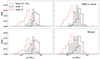 |
Fig. 1. Distribution of first-generation primary (left) and secondary (right) masses of dynamical BBHs that are retained within the cluster (upper panels) and merge (lower panels). We show the distributions from the Dragon-II direct N-body simulations (Arca Sedda et al. 2024a, gray shaded area) and in FASTCLUSTER, produced by sampling A (blue dashed line) and B (red dot-dashed line). |
For both sampling criteria, we applied a further correction to the BH masses based on the supernova kick, calculated as (Mapelli et al. 2021):
 (5)
(5)
where mBH is the BH mass, ⟨mNS⟩ = 1.33 M⊙ is the average neutron star mass (Özel & Freire 2016), and vH05 is randomly drawn from a Maxwellian distribution with a root-mean square of 265 km s−1. If one member of the BBH received a kick of larger than vesc (Eq. (1)), we assumed that was ejected from the cluster, and did not integrate its dynamics any further.
We sampled the dimensionless spin magnitudes (χ1 and χ2) of the BHs from a Maxwellian distribution with root-mean square σχ = 0.1. We chose this distribution as a toy model, because there is no consensus on the spin distribution from first principles (see, e.g., Fuller & Ma 2019; Belczynski et al. 2020; Bavera et al. 2020; Périgois et al. 2023). Our choice qualitatively matches the spin distribution inferred by the LIGO–Virgo–KAGRA (LVK) Collaboration (Abbott et al. 2023b). We drew spin directions isotropic over the sphere, because dynamical interactions reset any spin alignments with the orbital angular momentum of the binary system.
Finally, we sampled the initial orbital eccentricity from a thermal probability distribution (Heggie 1975):
 (6)
(6)
and the semi-major axis from:
![Mathematical equation: $$ \begin{aligned} p(a) \propto a^{-1} \quad a \in {[1,10^{3}]} \, {R_{\odot }}. \end{aligned} $$](/articles/aa/full_html/2024/08/aa49272-24/aa49272-24-eq7.gif) (7)
(7)
As soft binaries tend to be disrupted by dynamical interactions (Heggie 1975), we first checked whether the newly generated binary was hard. If it was not, we did not integrate it any further, assuming it was disrupted by further interactions (Mapelli et al. 2021).
2.2.2. Testing the BH pairing functions with N-body models
In the following, we compare the distributions of BBHs given by the BBH pairing functions introduced in Sect. 2.2.1 with those from the N-body models by Arca Sedda et al. (2023b, 2024a,b), whose stellar and binary evolution prescriptions are also based on the formulae of (Hurley et al. 2000, 2002; see Kamlah et al. 2022 for more details). Specifically, we ran 106 models at the same metallicity as the N-body simulations (Z = 0.0005), and compared the distributions of first-generation BBHs that are retained within the cluster and that merge.
As shown in Fig. 1, the BBH distributions from N-body simulations lie somewhere in between the two considered pairing functions. The sampling A captures the expected dynamical trend, which favors the coupling of the most massive BHs. The position of the dynamical peak, however, is very sensitive to the underlying stellar evolutionary models. For this reason, different prescriptions can result in discrepancies at the high-mass end of the distribution. The N-body models also display a long high-mass tail due to gas accretion from companion stars. The sampling B displays a milder increase at higher masses, without the presence of a clear peak, as in the N-body models. However, this case can reproduce the trend at low masses, despite the different BH mass distribution at first generation.
Our comparison suggests that there are many uncertainties related to the BH pairing function that are due to the impact of primordial binaries (which are not included in our formalism), deviations with respect to energy equipartition (Spera et al. 2016), stellar and binary evolution models, BH–star interactions, and possibly stochastic fluctuations. For example, Arca Sedda et al. (2024a) assume that BHs can accrete up to 50% of the stellar mass during BH–star collisions. This results in the high-mass tail above the lower limit of the pair-instability mass gap, which is not present in our models. At the same time, the prescriptions of these latter authors for (pulsational) pair-instability supernovae produce a peak that is ∼30% lower than in our models at Z = 0.0005. These differences affect the resulting primary mass distribution, which is expected to peak toward the 1g BH mass upper limit. At lower masses, that is, at ≲30 M⊙, different schemes for core collapse supernovae affect the BH mass distribution. In this case, the delayed model used by Arca Sedda et al. (2024a) does not predict any mass gap below 5 M⊙, in contrast to the rapid model used for our runs. These differences mainly affect the secondary masses, which can extend to the lower limit of the 1g BH mass distribution.
A detailed exploration of all these factors goes beyond the scope of this work and merits a dedicated study. In the following, we show the results of sampling both A and B to bracket these uncertainties.
2.2.3. BBH evolution
We evolve the semi-major axis a and orbital eccentricity e of hard BBHs through the formalism described in Eq. (16) of Mapelli et al. (2021), that is, by integrating a system of ordinary differential equations for a and e that takes into account dynamical hardening and GW decay or circularization. When a BBH merges within a Hubble time (13.6 Gyr), we estimate the mass and spin of the merger remnant from the fitting formulas provided by Jiménez-Forteza et al. (2017). Also, we calculate the relativistic kick magnitude vK (Lousto et al. 2012). The merger remnant is retained inside its parent cluster if the relativistic kick magnitude vK < vesc, with vesc given by Eq. (1). In this case, we model the dynamical formation of an Nth generation BBH and its evolution, as described in Mapelli et al. (2022).
We iterate the hierarchical merger process until we reach one of the following conditions: the merger remnant is ejected from the cluster, the cluster evaporates, no BHs remain within the cluster, or we reach the Hubble time.
2.2.4. Nth-generation secondary mass sampling
We sampled the Nth-generation (ng) secondary BHs following the criteria introduced in Sect. 2.2.1 for the 1g BBHs. For the sampling A, we drew m2 from Eq. (3) by setting m1 to the mass of the ng primary. As this model relies on the definition of a probability density function, which cannot be constrained in a direct way for ng BHs; we only consider ng1g BBHs.
For the sampling B, we drew the secondary mass from Eq. (4). We considered two different cases, hereafter ngng and ng1g. In the ngng case, we assumed that the secondary BH mass m2 ranges within [mmin, m1, ng], where mmin is the minimum BH mass and m1, ng is the mass of the primary BH belonging to the Nth generation. This yields the possibility that the secondary BH comes from previous mergers, as done by Mapelli et al. (2021).
In the ng1g case, we assumed that the secondary is always a 1g BH, and m2 ∈ [mmin, max(m1, 1g)), where max(m1, 1g) is the maximum mass of a primary first-generation BH. This assumption leads to smaller mass ratios at ng > 1, because our secondary sampling criterion (Eq. (4)) favors larger masses but BBHs with q = 1 can no longer form due to the increasing primary mass. In turn, this can result in larger relativistic recoil during a merger, the magnitude of which decreases in more symmetric configurations (González et al. 2007; Schnittman & Buonanno 2007; Herrmann et al. 2007).
2.3. Merger rate
We evaluated the merger rate density of dynamical BBHs in GCs (Mapelli et al. 2022) as:
![Mathematical equation: $$ \begin{aligned} \mathcal{R} (z) = \int _{z_{\rm max}}^{z} \,\psi (z^\prime )\, \frac{\mathrm{d}t(z^\prime )}{\mathrm{d}z^\prime } \left[\int _{Z_{\rm min}}^{Z_{\rm max}} \eta (Z)\,\mathcal{F} (z^\prime ,z,Z) \,\mathrm{d}Z\right]\,\mathrm{d}z^\prime , \end{aligned} $$](/articles/aa/full_html/2024/08/aa49272-24/aa49272-24-eq8.gif) (8)
(8)
where t(z) is the look-back time at redshift z, ψ(z′) is the GC formation rate density at redshift z′, and Zmin(z′) (Zmax(z′)) is the minimum (maximum) metallicity of stars formed at redshift z′. The merger efficiency η is defined as the total number of BBHs of a given population that merge within a Hubble time divided by the total initial stellar mass of that population (Giacobbo et al. 2018; Klencki et al. 2018). Finally, ℱ(z′,z, Z) is the merger rate of BBHs that form at redshift z′ from stars with metallicity Z and merge at redshift z, normalized to all BBHs that form from stars with metallicity Z. We calculated the cosmological parameters (H0, ΩM and ΩΛ) from Planck Collaboration XIII (2016).
We assumed a Gaussian distribution to model the GC formation rate as a function of redshift:
![Mathematical equation: $$ \begin{aligned} \psi (z)=\mathcal{B} _{\rm GC}\,\exp {\left[-\frac{(z-z_{\rm GC})^2}{(2\,\sigma _{\rm GC}^2)}\right]}, \end{aligned} $$](/articles/aa/full_html/2024/08/aa49272-24/aa49272-24-eq9.gif) (9)
(9)
with its maximum at zGC = 3.2 and a spread of σGC = 1.5 (Mapelli et al. 2022). The fiducial normalization constant is ℬGC = 2 × 10⁻⁴ M⊙ Mpc−3 yr−1, consistently with El-Badry et al. (2019) and Reina-Campos et al. (2019).
We calculated the merger efficiency η(Z) as:
 (10)
(10)
where, for a given Z, 𝒩merg, sim(Z) is the number of simulated merging BHs, 𝒩sim(Z) is the number of simulated BHs, 𝒩BH is the total number of BHs associated with a given metallicity, and M⋆(Z) is the total initial stellar mass for a given metallicity Z. We estimated M⋆(Z) as the sum of the initial total mass of all simulated star clusters with a given Z, and 𝒩BH(Z) as the number of BHs that we expect from a stellar population following a Kroupa mass function between 0.1 and 150 M⊙ (Kroupa 2001), assuming that all stars with a zero-age main sequence mass of ≥20 M⊙ are BH progenitors (Heger et al. 2003).
We calculated
 (11)
(11)
where d𝒩(z′,z, Z)/dt is the total number of BBHs that form at redshift z′ with metallicity Z and merge at redshift z per unit time, and 𝒩TOT(Z) is the total number of BBH mergers with progenitor’s metallicity Z. We evaluated the dispersion around the mass-weighted metallicity by assuming a log-normal distribution for the metallicity:
![Mathematical equation: $$ \begin{aligned} p(z^\prime , Z) = \frac{1}{\sqrt{2 \pi \, \sigma _{Z}^2}}\, \exp \left\{ {-\frac{\left[\log {(Z(z^\prime )/Z_\odot )} - {\langle \log {Z(z^\prime )/Z_\odot }\rangle }\right]^2}{2\,\sigma _{\rm Z}^2}}\right\} , \end{aligned} $$](/articles/aa/full_html/2024/08/aa49272-24/aa49272-24-eq12.gif) (12)
(12)
where
 (13)
(13)
We took the average metallicity ⟨Z(z)/Z⊙⟩ from Madau & Fragos (2017) and assumed a standard deviation of σZ = 0.3 (Mapelli et al. 2022). We refer the interested reader to Mapelli et al. (2022) for all the details of the calculation and the underlying assumptions.
2.4. Description of the runs
For our GC models, we considered seven metallicities: Z = 0.0002, 0.0008, 0.002, 0.004, 0.006, 0.012, and 0.02. We performed a denser sampling between 0.002 and 0.02, where the metallicity variation has a stronger impact on the 1g BH distribution.
For each metallicity, we ran three sets of N = 5 × 10⁶ BBHs, corresponding to the mass sampling criteria introduced in Sects. 2.2.1 and 2.2.4. In the following, we refer to these three models as follows:
-
Model A: we draw the primary and secondary mass of 1g BBHs according to sampling A (Sect. 2.2.1), and we sample the secondary mass of hierarchical BBHs according to the ng1g criterion (Sect. 2.2.4);
-
Model B: we draw the primary and secondary mass of 1g BBHs according to sampling B (Sect. 2.2.1), and we sample the secondary mass of hierarchical BBHs according to the ngng criterion (Sect. 2.2.4); that is, we assume that the secondary can be a ng BH;
-
Model C: we draw the primary and secondary mass of 1g BBHs according to sampling B (Sect. 2.2.1), and we sample the secondary mass of hierarchical BBHs according to the ng1g criterion (Sect. 2.2.4); that is, we assume that the secondary is always a 1g BH.
We considered three evolutionary cases for the host GCs:
-
NoEv: the absence of star cluster evolution.
-
Evol: star cluster evolution in isolation.
-
Tidal: star cluster evolution in the presence of a tidal field.
To highlight the impact of GC evolution, for each evolutionary case we set the same initial seed of our random generations. In total, we ran 189 different models, corresponding to 9.45 × 10⁸ 1g BBHs. Table 1 reports the details of our models.
Summary of the runs.
3. Results
3.1. Impact of GC evolution
Figure 2 shows the impact of GC evolution on the primary BH mass distribution for different BBH generations. Independently of the selected mass sampling, GC evolution quenches hierarchical mergers at the third generation. This is at least one generation earlier than what is predicted by nonevolving GC models. Only in model B can GCs still produce 4g mergers, but their efficiency is reduced by a factor of ∼50 with respect to models where GC evolution is not taken into account. The maximum primary BH mass is ∼150 M⊙ if only ng1g mergers are considered, while for model B it can be as high as ∼300 M⊙.
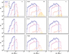 |
Fig. 2. Primary BH mass distribution of BBH mergers for models A (left), B (center), and C (right) for the three evolutionary cases considered: NoEv (upper panels), Evol (middel panels), and Tidal (lower panels). Different colors correspond to different BH generations: 1g (blue), 2g (purple), 3g (salmon), and > 3g (yellow) BHs. Here, we show our models with Z = 0.0002 because they are representative of metal-poor GCs in the Galactic halo (Muratov & Gnedin 2010). |
The process that mainly quenches the hierarchical chain is the internal GC relaxation. Cluster expansion, powered by the central BH subsystem, reduces the GC central density and, in turn, the dynamical hardening rate. GC expansion and mass loss also lower the cluster escape velocity, favoring the ejection by relativistic recoil upon merger. For 1g BBH mergers, the percentage of ejected BH remnants increases from 83% to 92% when GC evolution is implemented. Only in GCs with an initial vesc ≳ 80 km s−1 does this percentage fall below 80%.
As shown in Fig. 2, the external tidal field does not affect the hierarchical assembly significantly. However, we point out that our implementation is relatively conservative: it does not account for disk and bulge shocking, and for possible encounters with molecular clouds, which can significantly enhance star cluster dissolution (Gieles et al. 2006). Furthermore, here we only consider GCs at a galactocentric distance of 8 kpc from the center of a Milky-Way like galaxy.
3.2. Impact of the pairing function
The BBH mass pairing criterion deeply affects the mass distribution of BBH mergers (Fig. 2). In our model A, m1 is skewed towards the maximum 1g BH mass, and there are almost no mergers with m1 ≲ 15 M⊙. In contrast, models B and C display a smoother primary mass distribution, extending down to the minimum BH mass in our models (5 M⊙).
Figure 3 compares the mass ratio distributions at different generations. At 1g, all the mass samplings result in similar distributions, with a monotonic trend and a strong preference for q = 1. For higher generations, the mass ratio distribution displays significant differences. In model A, the ng secondary mass is likely to be m2 ∼ max(m1, 1g), because this sampling favors the most massive BHs. As m1, 2g ∼ 2max(m1, 1g), the 2g mass ratio distribution peaks at ∼0.5, and the 3g distribution spreads around 1/3. In model B, the mass ratios display similar distributions at all generations, because m2 is determined from Eq. (4). In model C, the distribution shows a flatter trend after the second generation, as m1, 3g ≳ max(m1, 1g) and mass ratios close to 1 are no longer possible.
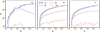 |
Fig. 3. Mass ratio distributions of BBH mergers for models A (left), B (center), and C (right) in the Tidal evolutionary case. Different colors correspond to different BH generations: 1g (blue), 2g (purple), 3g (salmon), and > 3g (yellow) BHs. Here, we show models with Z = 0.0002. |
We evaluate the impact of ng1g mergers on BH retention by comparing the fraction of ejected BH remnants for models B and C, where the BBH masses only differ for the secondary BH mass sampling at ng > 1. For model C, the fraction of BHs ejected by the GW relativistic recoil increases by 1% at 2g and by 4% at 3g, indicating that the ng1g assumption plays only a minor role in their retention.
3.3. Primary BH mass merger rate density in the Local Volume
Figure 4 shows the primary mass-differential-merger-rate density in the Local Volume. To obtain this quantity, we integrated the merger-rate density as described in Sect. 2.3, taking into account different progenitor metallicities. Overall, despite the large differences for low primary BH masses (m1 ≤ 20 M⊙), all of our models (A, B, C) reproduce both the peak at m1 ≈ 30 − 40 M⊙ and the high-mass tail (> 50 M⊙) reported by the LVK Collaboration (Abbott et al. 2016).
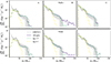 |
Fig. 4. Primary BH mass differential merger rate density in the Local Volume for models A (left), B (center), and C (right) for the NoEv (upper panels) and Tidal (lower panels) cases. We show the mass distribution resulting from 1g mergers (yellow dash-dotted line), 1g and 2g mergers (green dashed line), and from all BBH generations together (purple solid line). The black dashed line is the median value of the POWER LAW + PEAK model, as inferred from GWTC-3 (Abbott et al. 2023b). The gray shaded areas are the corresponding 90% credible intervals. In this and the following figures, the black line and shaded gray areas are shown only for a qualitative comparison, because our simulations do not assume the parametric models adopted by the LVK. |
In all of our models, the high-mass tail of the primary BH mass distribution (m1 > 40 M⊙) is almost uniquely populated by hierarchical mergers. The host GC evolution quenches the contribution of hierarchical mergers to the merger-rate density, because it results in a less efficient hardening rate at late times.
The BH sampling criterion plays a key role in determining the primary mass distribution. All the models are able to account for the high-mass tail inferred by the LVK Collaboration (Abbott et al. 2023a,b), independently of the sampling criteria. At lower masses, instead, the considered sampling criteria differ dramatically: models B and C predict a larger BBH population at lower masses, with a main peak at ≈10 M⊙ and a monotonically decreasing trend. Also, they approximately match the second peak at ≈35 M⊙.
In contrast, model A does not produce any peak at ≈10 M⊙. This model results in a main peak extending from ≈25 M⊙ to ≈50 M⊙, which roughly encloses the 35 M⊙ peak inferred from GW observations. Here, the peak is mostly due to 1g BBH mergers. A secondary peak due to 2g BBH mergers is present at ≈70 − 80 M⊙. These results are consistent with those from Antonini et al. (2023), who considered the same mass sampling criterion, but a power-law BH mass function.
This demonstrates the importance of quantifying the uncertainties related to the BH pairing function: according to models B and C, BBH mergers from GCs can account for a larger fraction of the LVK population, whereas model A suggests that GCs can produce only a subpopulation with a primary BH mass of ≳30 M⊙.
3.4. Evolution of the primary BH mass with redshift
Figure 5 shows the dependence of the primary BH mass distribution on redshift. In all our models, the primary mass distribution evolves with redshift: BH mergers with m1 < 20 M⊙ (m1 > 30 M⊙) are progressively quenched (become more common) as redshift increases. The reason for this trend is the relative contribution of different progenitor-star metallicities at different redshifts (see Appendix C).
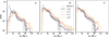 |
Fig. 5. Probability distribution function of primary BH masses at redshift z = 0 (black solid line), z = 1 (purple dotted line), z = 2 (salmon dashed line), and z = 3 (yellow dash-dotted line) for models A (left), B (center), and C (right) in the Tidal evolutionary case. In model B, the distribution extends to higher masses, but the plot is truncated at 150 M⊙ to improve the readability of the figure. The black dashed line is the median value of the POWER LAW + PEAK model, as inferred from GWTC-3 (Abbott et al. 2023b). The gray shaded areas are the corresponding 90% credible intervals. |
In model A, the main peak of the distribution shifts from ∼35 M⊙ at z = 0 to ∼50 M⊙ at z = 3. As this mass sampling is skewed toward the maximum mass of the 1g BH spectrum, the larger contribution of subsolar metallicities for z > 0 produces different peaks, depending on the dominant metallicity at the considered redshift. In models B and C, the primary BH mass distribution for z > 0 is no longer monotonically decreasing, but shows a depletion at 10 M⊙, and a main peak at 20 M⊙.
Previous works suggest the existence of a weak trend (Fishbach et al. 2021), or even a strong correlation (Rinaldi et al. 2024) between primary BH mass and redshift. Our result indicates that dynamically assembled BBH mergers in GCs may account for such a trend. Finding a more top-heavy BH mass function at higher redshift (z ≳ 1) would therefore strongly suggest a dynamical origin of these BBH mergers. Next-generation ground-based GW detectors will be able to address this point (Reitze et al. 2019; Maggiore et al. 2020; Evans et al. 2021; Branchesi et al. 2023).
4. Discussion
4.1. Comparison with isolated mergers
Here, we compare the primary mass, mass ratio, and spin distribution of BBHs in GCs to those predicted from isolated BBH mergers evolved with the same stellar evolution prescriptions as those used in our dynamical runs.
We take the isolated BBH mergers from a simulation run with MOBSE (Mapelli et al. 2017; Giacobbo et al. 2018). This simulation consists of 1.8 × 10⁸ binary systems comprising nine metallicities (Z = 0.0002, 0.0008, 0.002, 0.004, 0.006, 0.008, 0.012, 0.016, 0.02). We drew the zero-age main sequence mass of the primary stars from a Kroupa (Kroupa 2001) initial mass function between 5 and 150 M⊙. We sampled the initial mass ratios, orbital eccentricity, and semi-major axis from the distribution by Sana et al. (2012), which are fits to observations of massive binary stars. We included core-collapse and pair-instability supernovae as described in Sect. 2.2.1 and we integrated each binary system accounting for wind mass transfer, Roche-lobe overflow, common envelope (assuming efficiency α = 3), tides, and GW decay as described in Giacobbo et al. (2018). In order to calculate the merger rate density of isolated BBHs, we used Eq. (8), assuming the cosmic star formation rate density ψ(z) and metallicity evolution from Madau & Fragos (2017). We refer to Santoliquido et al. (2020, 2021) for details.
4.1.1. Primary mass and mass ratios
Figure 6 shows the primary mass and mass-ratio distribution of BBH mergers from GCs and isolated binaries. As expected, primary BH masses from isolated binaries peak at 10 M⊙, matching the main peak of the LVK population (Abbott et al. 2023b). Below ≈40 M⊙, the main difference between isolated BBHs and models B and C is the relative importance of the 10 M⊙ peak, which is a factor of about 3 higher in isolated binaries. In contrast, model A is dramatically different from isolated BBHs even at low primary BH masses.
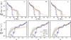 |
Fig. 6. Primary BH mass (upper panels) and mass ratio (lower panels) differential merger rate density in the Local Volume for models A (left), B (center), and C (right) in the Tidal evolutionary case. We show the mass distribution resulting from isolated BBH mergers (blue solid line), 1g BBH mergers in GCs (yellow dash-dotted line), and all BBH mergers in GCs (including hierarchical mergers, salmon dashed line). The black dashed line is the median value of the POWER LAW + PEAK model inferred from GWTC-3 (Abbott et al. 2023b). The gray shaded areas are the corresponding 90% credible intervals: these are shown only for a qualitative comparison, because our simulations do not assume the parametric models adopted by the LVK. We refer to Appendix D for a quantitative analysis. |
For large primary masses (≳40 M⊙), all of our GC models differ from the isolated BBH model, as the latter cannot account for the high-mass tail, while the former produce high-mass BHs via hierarchical mergers. The distribution of mass ratios (lower panel of Fig. 6) shows that unequal-mass BBHs are more common in our dynamical BBHs with respect to isolated BBHs. The mass ratios from dynamical BBHs are qualitatively consistent with the lower end of the distribution inferred from the parametric model adopted by the LVK Collaboration (Abbott et al. 2023b). Dynamical mergers dominate the distribution at low q values. In contrast, the distribution from the isolated channel cannot explain the LVK rate for q < 0.5. In this case, the steep decrease in the mass ratio distribution at low q stems from common-envelope evolution, which is responsible for BBH hardening in our models and favors the formation of equal-mass binaries.
At high values of q, model A shows a flatter trend than both models B and C, and, for q ≳ 0.8, is about one order of magnitude below the median value inferred by the LVK Collaboration for the adopted parametric model (Abbott et al. 2023b). In contrast, models B and C display an increasing trend throughout the entire range in q and are always within the 90% credible interval of the LVK parametric model shown in the figure (Abbott et al. 2023b).
4.1.2. Spins
For each BBH merger, we estimated the effective spin (χeff) and the precessing spin (χp):
 (14)
(14)
where L is the orbital angular momentum of the BBH, B1 ≡ 2 + 3 q/2, and B2 ≡ 2 + 3/(2 q). S1⊥ and S2⊥ are the components of the spin vectors (S1 and S2) perpendicular to the orbital angular momentum. χeff characterizes a mass-averaged spin angular momentum in the direction parallel to the binaries orbital angular momentum, while χp approximately corresponds to the degree of in-plane spin, and traces the rate of relativistic precession of the orbital plane.
Figure 7 shows the distributions of χeff and χp from our models in the Tidal evolutionary case compared to the inferred distributions through the Gaussian spin model presented by Abbott et al. (2023b). The isolated channel mainly leads to the formation of low χp and positive χeff, because of angular momentum alignment driven by mass transfer and tidal effects. First-generation BBHs in GCs show a distribution of χeff that is symmetric around zero due to the assumption of isotropic spins, and a peak at χp ≈ 0.15. The spread of the distributions of χeff and χp depend on the initial value of the parameter σχ of the initial Maxwellian distribution, which, in our models is set to 0.1 (Sect. 2.2.1).
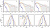 |
Fig. 7. Precessing (upper panels) and effective (lower panels) spin distribution of BBH mergers at redshift z = 0 for models A (left), B (center), and C (right) in the Tidal evolutionary case. We show the mass distribution resulting from isolated BBH mergers (blue solid line), 1g BBH mergers in GCs (yellow dash-dotted line), and BBH mergers in GCs, including hierarchical mergers (salmon dashed line). The black dashed line is the median value of the Gaussian spin model inferred from GWTC-3 (Abbott et al. 2023b). The gray shaded areas are the corresponding 90% credible intervals. |
Black holes from previous mergers typically display larger spins, resulting from the sum of their parent BBH orbital angular momentum and BH spins. This produces a spin distribution peaked at χ ∼ 0.7 (Gerosa & Berti 2017; Fishbach et al. 2017), and, in turn, a peak at χp = 0.7. In model B, where the contribution of 3g mergers is not negligible, a tail at χp ≈ 0.8 is present, which is due to the further spin increase in successive generations. Also, the high spins produced by hierarchical mergers can extend the distribution of χeff to much lower and higher values.
The population inferred from GWs is mostly consistent with slowly rotating BHs (Callister et al. 2022), but the decrease at high spins is milder than what is expected from 1g mergers only, according to our models. At the same time, high absolute values of χeff from hierarchical mergers are not ruled out by current GW detections. Given the current uncertainties on spin parameters, additional GW detections will be crucial to constrain a possible secondary peak in the distribution of χp due to hierarchical mergers.
4.2. Mixing fractions
As a simple but instructive exercise, we calculated the mixing fraction between two channels: BBHs born in GCs and BBHs formed in isolated binary systems. For the latter, we used the models described in Sect. 4.1. Here, we neglected the other dynamical channels for simplicity, because a two-channel analysis allows a more straightforward interpretation of the impact of the main model features. We refer to Mapelli et al. (2022) for a more sophisticated but somewhat less transparent four-channel analysis.
We calculated the probability of recovering the parameters θ = {ℳchirp, q, z, χeff, χp} of the observed LVK events3 (Abbott et al. 2023b) given the mixing fraction fGC and the other hyperparameters of our models λ:
 (15)
(15)
According to this formalism, a mixing fraction fGC = 0 (fGC = 1) means that all BBHs are born from isolated binary systems (GCs). In our analysis, we considered 58 BBH events from Abbott et al. (2023a) with a probability of having an astrophysical origin of pastro > 0.9 and a false-alarm rate (FAR) of < 0.25 yr−1. We describe our hierarchical Bayesian framework in Appendix D. With this approach, we also take into account observational biases, associating a detection probability to our simulated catalogs. This allows us to make a fair comparison between our models and LVK data.
Figure 8 shows the probability distribution function (PDF) of the GC mixing fraction fGC we obtain if we marginalize (upper panel) or do not marginalize over χeff and χp (lower panel). This figure shows a clear predominance of the GC channel if we include the spin parameters in the calculation of the mixing fraction, almost regardless of the GC model we assume. The main reason for this is that our isolated binary model tends to produce spins that are overly aligned with the orbital angular momentum in order to account for the majority of the LVK data (see Fig. 7 and Appendix D for details). This result confirms that the evolution of spin orientation during binary evolution is a key process (e.g., Stegmann & Antonini 2021; Callister et al. 2021b). As shown by Mapelli et al. (2022), this result is degenerate with the initial assumption on spin magnitudes. In particular, the choice of lower 1g spin magnitudes (e.g., σχ = 0.01) can lead to a higher contribution of the isolated BBHs to the mixing fraction.
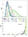 |
Fig. 8. Mixing fraction (fGC) probability distribution function. A mixing fraction fGC = 0 (fGC = 1) means that all BBHs are born from isolated binary systems (GCs). In the upper and lower panels, we and do not marginalize over the spin parameters χeff and χp in our analysis, respectively. All the models presented in this paper are shown with different colors, as described in the legend. |
If we do not include χeff and χp in our analysis, that is if we marginalize over them, the GC mixing fraction fGC decreases significantly, implying an important contribution of the isolated BBH channel. The contribution of the isolated BBHs when we neglect the spins mostly stems from the impact of m1. In fact, our isolated binary models have a preference for m1 ∼ 8 − 10 M⊙, which corresponds to the main peak in the LVK population (Fig. 6). In contrast, this peak is suppressed in all of our dynamical models, especially model A.
Model C – NoEv results in the largest GC mixing fraction among dynamical models if we neglect the spins (median value of fGC ≈ 0.4 for model C – NoEv), whereas models A and B cluster at lower values of fGC. This difference is more prone to stochastic fluctuations in our simulations. However, we note that model C – NoEv better reproduces the events with both a large value of chirp mass ℳchirp and a low value of q in the LVK data (Appendix D). Overall, the differences between models Evol, NoEv, and Tidal are negligible in the analysis of the mixing fractions.
5. Summary
We investigated the process of hierarchical mergers in GCs, accounting for the main physical processes that drive GC evolution, namely mass loss by stellar evolution, expansion powered by a central BH subsystem, and tidal stripping. We also bracket the uncertainties related to BH pairing functions on the predicted primary BH mass, mass ratio, and spin distribution.
We summarize our main results as follows.
-
Globular cluster expansion quenches the hierarchical BH assembly at the third generation. Our models predict a maximum BH mass of ∼140 M⊙ if the mergers only involve first-generation secondary BHs, and ∼300 M⊙ if we include the possibility of ng secondary BHs.
-
In all of our models, the hierarchical mergers dominate the primary BH mass distribution for m1 > 50 M⊙, and can reproduce the high-mass tail inferred from GW events.
-
The adopted mass pairing function deeply affects the low-mass end of the primary BH mass distribution. Model A suppresses the formation of low-mass BBHs, resulting in a main peak around m1 = 35 M⊙. In contrast, models B and C produce a peak in the primary BH mass function at m1 ∼ 10 M⊙ and then a monotonic decrease for larger masses.
-
The primary BH mass distribution evolves with redshift in all of our GC models, with a larger contribution from mergers with m1 ≥ 30 M⊙ at z ≥ 2, while low-mass BBH mergers are quenched at high redshift. This effect stems from the interplay between GC dynamics and stellar metallicity evolution.
-
Overall, despite the large differences for low primary BH masses (m1 ≤ 20 M⊙), all of our models (A, B, and C) match both the peak at m1 ≈ 30 − 40 M⊙ and the high-mass tail (> 50 M⊙) reported by the LVK Collaboration (Abbott et al. 2023b). This confirms the importance of star-cluster dynamics and hierarchical mergers in producing the most massive BBH mergers observed with LVK.
-
We compared the primary mass, mass ratio, and spin distribution of dynamical BBHs in GCs to those derived from isolated BBH mergers. Isolated binaries result in a three times greater contribution than models B and C at 10 M⊙, matching the main peak from LVK data. In contrast, dynamical mergers in GCs are necessary to reproduce the events with m1 > 50 M⊙ and q < 0.5. Also, hierarchical mergers imprint a secondary peak in the χp distribution and contribute to the positive and negative wings of the χeff distribution.
-
We calculated the mixing fraction between dynamical BBHs in GCs and isolated BBHs. Our predictions are very sensitive to the spin parameters, which favor a large fraction of dynamical BBH mergers in GCs (fGC > 0.6).
Our analysis confirms the importance of hierarchical mergers in matching the high-value tails of the primary BH mass (m1 ≥ 50 M⊙) and precession spin distributions (χp ∼ 0.7). We predict that the mass of BBH mergers in GCs increases with redshift, regardless of the uncertainties related to the BBH pairing function. The ongoing fourth observing run of the LVK and next-generation GW detectors will be an important test-bed for our key predictions.
FASTCLUSTER is an open-source code available at https://gitlab.com/micmap/fastcluster_open
MOBSE (Mapelli et al. 2017; Giacobbo et al. 2018) is a custom and upgraded version of BSE (Hurley et al. 2002), and is publicly available at https://gitlab.com/micmap/mobse_open
In our formalism, ℳchirp = (m1 m2)3/5 (m1 + m2)−1/5 is the BBH chirp mass.
CLUSTERBH is available at https://github.com/mgieles/clusterbh
 , where
  is the waveform and Sn the power spectral noise density.
Acknowledgments
We thank the anonymous referee for their comments, which helped us to improve this manuscript. We thank Mark Gieles and Fabio Antonini for sharing CLUSTERBH and for productive discussions. M.M., S.T., C.P., M.D. and M.P.V. acknowledge financial support from the European Research Council for the ERC Consolidator grant DEMOBLACK, under contract no. 770017. S.T., M.M. and M.P.V. also acknowledge financial support from the German Excellence Strategy via the Heidelberg Cluster of Excellence (EXC 2181 – 390900948) STRUCTURES. M.D. also acknowledges financial support from Cariparo foundation under grant 55440. M.A.S. acknowledges funding from the European Union’s Horizon 2020 research and innovation programme under the Marie Skłodowska-Curie grant agreement No. 101025436 (project GRACE-BH). M.C.A. acknowledges financial support from the Seal of Excellence @UNIPD 2020 program under the ACROGAL project.
References
- Aasi, J., Abbott, B. P., Abbott, R., et al. 2015, Class. Quant. Grav., 32, 074001 [Google Scholar]
- Abbott, B. P., Abbott, R., Abbott, T. D., et al. 2016, ApJ, 818, L22 [Google Scholar]
- Abbott, B. P., Abbott, R., Abbott, T. D., et al. 2019, Phys. Rev. X, 9, 031040 [Google Scholar]
- Abbott, R., Abbott, T. D., Abraham, S., et al. 2020a, ApJ, 896, L44 [Google Scholar]
- Abbott, R., Abbott, T. D., Abraham, S., et al. 2020b, Phys. Rev. Lett., 125, 101102 [Google Scholar]
- Abbott, R., Abbott, T. D., Abraham, S., et al. 2020c, ApJ, 900, L13 [NASA ADS] [CrossRef] [Google Scholar]
- Abbott, R., Abbott, T. D., Abraham, S., et al. 2021a, Phys. Rev. X, 11, 021053 [Google Scholar]
- Abbott, R., Abbott, T. D., Abraham, S., et al. 2021b, ApJ, 913, L7 [NASA ADS] [CrossRef] [Google Scholar]
- Abbott, R., Abbott, T. D., Acernese, F., et al. 2023a, Phys. Rev. X, 13, 041039 [Google Scholar]
- Abbott, R., Abbott, T. D., Acernese, F., et al. 2023b, Phys. Rev. X, 13, 011048 [NASA ADS] [Google Scholar]
- Abbott, R., Abbott, T. D., Acernese, F., et al. 2024, Phys. Rev. D, 109, 022001 [NASA ADS] [CrossRef] [Google Scholar]
- Acernese, F., Agathos, M., Agatsuma, K., et al. 2015, Class. Quant. Grav., 32, 024001 [Google Scholar]
- Antonini, F., & Gieles, M. 2020, MNRAS, 492, 2936 [CrossRef] [Google Scholar]
- Antonini, F., & Rasio, F. A. 2016, ApJ, 831, 187 [Google Scholar]
- Antonini, F., Gieles, M., & Gualandris, A. 2019, MNRAS, 486, 5008 [NASA ADS] [CrossRef] [Google Scholar]
- Antonini, F., Gieles, M., Dosopoulou, F., & Chattopadhyay, D. 2023, MNRAS, 522, 466 [NASA ADS] [CrossRef] [Google Scholar]
- Arca Sedda, M., Mapelli, M., Benacquista, M., & Spera, M. 2023a, MNRAS, 520, 5259 [NASA ADS] [CrossRef] [Google Scholar]
- Arca Sedda, M., Kamlah, A. W. H., Spurzem, R., et al. 2023b, MNRAS, 526, 429 [NASA ADS] [CrossRef] [Google Scholar]
- Arca Sedda, M., Kamlah, A. W. H., Spurzem, R., et al. 2024a, MNRAS, 528, 5119 [NASA ADS] [CrossRef] [Google Scholar]
- Arca Sedda, M., Kamlah, A. W. H., Spurzem, R., et al. 2024b, MNRAS, 528, 5140 [CrossRef] [Google Scholar]
- Ballone, A., Costa, G., Mapelli, M., et al. 2023, MNRAS, 519, 5191 [NASA ADS] [CrossRef] [Google Scholar]
- Bavera, S. S., Fragos, T., Qin, Y., et al. 2020, A&A, 635, A97 [NASA ADS] [CrossRef] [EDP Sciences] [Google Scholar]
- Belczynski, K., Ryu, T., Perna, R., et al. 2017, MNRAS, 471, 4702 [Google Scholar]
- Belczynski, K., Klencki, J., Fields, C. E., et al. 2020, A&A, 636, A104 [NASA ADS] [CrossRef] [EDP Sciences] [Google Scholar]
- Bianchini, P., van de Ven, G., Norris, M. A., Schinnerer, E., & Varri, A. L. 2016, MNRAS, 458, 3644 [NASA ADS] [CrossRef] [Google Scholar]
- Bouffanais, Y., Mapelli, M., Gerosa, D., et al. 2019, ApJ, 886, 25 [NASA ADS] [CrossRef] [Google Scholar]
- Bouffanais, Y., Mapelli, M., Santoliquido, F., et al. 2021, MNRAS, 507, 5224 [NASA ADS] [CrossRef] [Google Scholar]
- Branchesi, M., Maggiore, M., Alonso, D., et al. 2023, JCAP, 2023, 068 [CrossRef] [Google Scholar]
- Breen, P. G., & Heggie, D. C. 2013, MNRAS, 432, 2779 [NASA ADS] [CrossRef] [Google Scholar]
- Briel, M. M., Stevance, H. F., & Eldridge, J. J. 2023, MNRAS, 520, 5724 [Google Scholar]
- Callister, T. A., & Farr, W. M. 2024, Phys. Rev. X, 14, 021005 [NASA ADS] [Google Scholar]
- Callister, T. A., Haster, C.-J., Ng, K. K. Y., Vitale, S., & Farr, W. M. 2021a, ApJ, 922, L5 [NASA ADS] [CrossRef] [Google Scholar]
- Callister, T. A., Farr, W. M., & Renzo, M. 2021b, ApJ, 920, 157 [NASA ADS] [CrossRef] [Google Scholar]
- Callister, T. A., Miller, S. J., Chatziioannou, K., & Farr, W. M. 2022, ApJ, 937, L13 [NASA ADS] [CrossRef] [Google Scholar]
- Chattopadhyay, D., Stegmann, J., Antonini, F., Barber, J., & Romero-Shaw, I. M. 2023, MNRAS, 526, 4908 [NASA ADS] [CrossRef] [Google Scholar]
- Costa, G., Bressan, A., Mapelli, M., et al. 2021, MNRAS, 501, 4514 [NASA ADS] [CrossRef] [Google Scholar]
- Costa, G., Ballone, A., Mapelli, M., & Bressan, A. 2022, MNRAS, 516, 1072 [NASA ADS] [CrossRef] [Google Scholar]
- Dehnen, W. 1993, MNRAS, 265, 250 [NASA ADS] [CrossRef] [Google Scholar]
- Di Carlo, U. N., Giacobbo, N., Mapelli, M., et al. 2019, MNRAS, 487, 2947 [NASA ADS] [CrossRef] [Google Scholar]
- Di Carlo, U. N., Mapelli, M., Bouffanais, Y., et al. 2020, MNRAS, 497, 1043 [NASA ADS] [CrossRef] [Google Scholar]
- El-Badry, K., Quataert, E., Weisz, D. R., Choksi, N., & Boylan-Kolchin, M. 2019, MNRAS, 482, 4528 [Google Scholar]
- Evans, M., Adhikari, R. X., Afle, C., et al. 2021, arXiv e-prints [arXiv:2109.09882] [Google Scholar]
- Farah, A. M., Edelman, B., Zevin, M., et al. 2023, ApJ, 955, 107 [NASA ADS] [CrossRef] [Google Scholar]
- Farmer, R., Renzo, M., de Mink, S. E., Marchant, P., & Justham, S. 2019, ApJ, 887, 53 [Google Scholar]
- Farmer, R., Renzo, M., de Mink, S. E., Fishbach, M., & Justham, S. 2020, ApJ, 902, L36 [CrossRef] [Google Scholar]
- Farrell, E., Groh, J. H., Hirschi, R., et al. 2021, MNRAS, 502, L40 [NASA ADS] [CrossRef] [Google Scholar]
- Fishbach, M., Holz, D. E., & Farr, B. 2017, ApJ, 840, L24 [NASA ADS] [CrossRef] [Google Scholar]
- Fishbach, M., Holz, D. E., & Farr, W. M. 2018, ApJ, 863, L41 [NASA ADS] [CrossRef] [Google Scholar]
- Fishbach, M., Doctor, Z., Callister, T., et al. 2021, ApJ, 912, 98 [NASA ADS] [CrossRef] [Google Scholar]
- Fragione, G., & Rasio, F. A. 2023, ApJ, 951, 129 [NASA ADS] [CrossRef] [Google Scholar]
- Fryer, C. L., Belczynski, K., Wiktorowicz, G., et al. 2012, ApJ, 749, 91 [Google Scholar]
- Fuller, J., & Ma, L. 2019, ApJ, 881, L1 [Google Scholar]
- Georgiev, I. Y., Puzia, T. H., Hilker, M., & Goudfrooij, P. 2009, MNRAS, 392, 879 [NASA ADS] [CrossRef] [Google Scholar]
- Gerosa, D., & Berti, E. 2017, Phys. Rev. D, 95, 124046 [NASA ADS] [CrossRef] [Google Scholar]
- Gerosa, D., & Fishbach, M. 2021, Nat. Astron., 5, 749 [NASA ADS] [CrossRef] [Google Scholar]
- Giacobbo, N., Mapelli, M., & Spera, M. 2018, MNRAS, 474, 2959 [Google Scholar]
- Gieles, M., & Baumgardt, H. 2008, MNRAS, 389, L28 [NASA ADS] [Google Scholar]
- Gieles, M., Portegies Zwart, S. F., Baumgardt, H., et al. 2006, MNRAS, 371, 793 [Google Scholar]
- Gieles, M., Heggie, D. C., & Zhao, H. 2011, MNRAS, 413, 2509 [Google Scholar]
- González, J. A., Sperhake, U., Brügmann, B., Hannam, M., & Husa, S. 2007, Phys. Rev. Lett., 98, 091101 [NASA ADS] [CrossRef] [Google Scholar]
- Goodman, J. 1984, ApJ, 280, 298 [NASA ADS] [CrossRef] [Google Scholar]
- Harris, W. E. 1996, AJ, 112, 1487 [Google Scholar]
- Harris, W. E., Harris, G. L. H., & Alessi, M. 2013, ApJ, 772, 82 [Google Scholar]
- Heger, A., Fryer, C. L., Woosley, S. E., Langer, N., & Hartmann, D. H. 2003, ApJ, 591, 288 [CrossRef] [Google Scholar]
- Heggie, D. C. 1975, MNRAS, 173, 729 [NASA ADS] [CrossRef] [Google Scholar]
- Heggie, D., & Hut, P. 2003, The Gravitational Million-Body Problem: A Multidisciplinary Approach to Star Cluster Dynamics (Cambridge: Cambridge University Press) [Google Scholar]
- Hendriks, D. D., van Son, L. A. C., Renzo, M., Izzard, R. G., & Farmer, R. 2023, MNRAS, 526, 4130 [NASA ADS] [CrossRef] [Google Scholar]
- Hénon, M. 1961, Ann. Astrophys., 24, 369 [Google Scholar]
- Herrmann, F., Hinder, I., Shoemaker, D., & Laguna, P. 2007, Class. Quant. Grav., 24, S33 [NASA ADS] [CrossRef] [Google Scholar]
- Hurley, J. R., Pols, O. R., & Tout, C. A. 2000, MNRAS, 315, 543 [Google Scholar]
- Hurley, J. R., Tout, C. A., & Pols, O. R. 2002, MNRAS, 329, 897 [Google Scholar]
- Jiménez-Forteza, X., Keitel, D., Husa, S., et al. 2017, Phys. Rev. D, 95, 064024 [CrossRef] [Google Scholar]
- Kamlah, A. W. H., Leveque, A., Spurzem, R., et al. 2022, MNRAS, 511, 4060 [NASA ADS] [CrossRef] [Google Scholar]
- Klencki, J., Moe, M., Gladysz, W., et al. 2018, A&A, 619, A77 [NASA ADS] [CrossRef] [EDP Sciences] [Google Scholar]
- Kremer, K., Spera, M., Becker, D., et al. 2020, ApJ, 903, 45 [NASA ADS] [CrossRef] [Google Scholar]
- Kritos, K., Strokov, V., Baibhav, V., & Berti, E. 2022, arXiv e-prints [arXiv:2210.10055] [Google Scholar]
- Kritos, K., Berti, E., & Silk, J. 2023, Phys. Rev. D, 108, 083012 [NASA ADS] [CrossRef] [Google Scholar]
- Kroupa, P. 2001, MNRAS, 322, 231 [NASA ADS] [CrossRef] [Google Scholar]
- Loredo, T. J. 2004, AIP Conf. Proc., 735, 195 [CrossRef] [Google Scholar]
- Lousto, C. O., Zlochower, Y., Dotti, M., & Volonteri, M. 2012, Phys. Rev. D, 85, 084015 [NASA ADS] [CrossRef] [Google Scholar]
- Madau, P., & Fragos, T. 2017, ApJ, 840, 39 [Google Scholar]
- Maggiore, M., Van Den Broeck, C., Bartolo, N., et al. 2020, JCAP, 2020, 050 [CrossRef] [Google Scholar]
- Mandel, I., Farr, W. M., & Gair, J. R. 2019, MNRAS, 486, 1086 [Google Scholar]
- Mapelli, M., Giacobbo, N., Ripamonti, E., & Spera, M. 2017, MNRAS, 472, 2422 [NASA ADS] [CrossRef] [Google Scholar]
- Mapelli, M., Spera, M., Montanari, E., et al. 2020, ApJ, 888, 76 [NASA ADS] [CrossRef] [Google Scholar]
- Mapelli, M., Dall’Amico, M., Bouffanais, Y., et al. 2021, MNRAS, 505, 339 [CrossRef] [Google Scholar]
- Mapelli, M., Bouffanais, Y., Santoliquido, F., Arca Sedda, M., & Artale, M. C. 2022, MNRAS, 511, 5797 [NASA ADS] [CrossRef] [Google Scholar]
- Marchant, P., & Moriya, T. J. 2020, A&A, 640, L18 [EDP Sciences] [Google Scholar]
- Marchant, P., Renzo, M., Farmer, R., et al. 2019, ApJ, 882, 36 [Google Scholar]
- Miller, M. C., & Hamilton, D. P. 2002, MNRAS, 330, 232 [Google Scholar]
- Muratov, A. L., & Gnedin, O. Y. 2010, ApJ, 718, 1266 [Google Scholar]
- O’Leary, R. M., Rasio, F. A., Fregeau, J. M., Ivanova, N., & O’Shaughnessy, R. 2006, ApJ, 637, 937 [CrossRef] [Google Scholar]
- O’Leary, R. M., Meiron, Y., & Kocsis, B. 2016, ApJ, 824, L12 [CrossRef] [Google Scholar]
- Özel, F., & Freire, P. 2016, ARA&A, 54, 401 [Google Scholar]
- Périgois, C., Mapelli, M., Santoliquido, F., Bouffanais, Y., & Rufolo, R. 2023, Universe, 9, 507 [CrossRef] [Google Scholar]
- Planck Collaboration XIII. 2016, A&A, 594, A13 [NASA ADS] [CrossRef] [EDP Sciences] [Google Scholar]
- Portegies Zwart, S. F., McMillan, S. L. W., & Gieles, M. 2010, ARA&A, 48, 431 [NASA ADS] [CrossRef] [Google Scholar]
- Quinlan, G. D., & Shapiro, S. L. 1990, ApJ, 356, 483 [NASA ADS] [CrossRef] [Google Scholar]
- Reina-Campos, M., Kruijssen, J. M. D., Pfeffer, J. L., Bastian, N., & Crain, R. A. 2019, MNRAS, 486, 5838 [NASA ADS] [CrossRef] [Google Scholar]
- Reitze, D., Adhikari, R. X., Ballmer, S., et al. 2019, BAAS, 51, 35 [NASA ADS] [Google Scholar]
- Renzo, M., Cantiello, M., Metzger, B. D., & Jiang, Y. F. 2020, ApJ, 904, L13 [NASA ADS] [CrossRef] [Google Scholar]
- Rinaldi, S., Del Pozzo, W., Mapelli, M., Lorenzo-Medina, A., & Dent, T. 2024, A&A, 684, A204 [NASA ADS] [CrossRef] [EDP Sciences] [Google Scholar]
- Sana, H., de Mink, S. E., de Koter, A., et al. 2012, Science, 337, 444 [Google Scholar]
- Santoliquido, F., Mapelli, M., Bouffanais, Y., et al. 2020, ApJ, 898, 152 [Google Scholar]
- Santoliquido, F., Mapelli, M., Giacobbo, N., Bouffanais, Y., & Artale, M. C. 2021, MNRAS, 502, 4877 [NASA ADS] [CrossRef] [Google Scholar]
- Schnittman, J. D., & Buonanno, A. 2007, ApJ, 662, L63 [Google Scholar]
- Spera, M., & Mapelli, M. 2017, MNRAS, 470, 4739 [Google Scholar]
- Spera, M., Mapelli, M., & Jeffries, R. D. 2016, MNRAS, 460, 317 [NASA ADS] [CrossRef] [Google Scholar]
- Spitzer, L. 1969, ApJ, 158, L139 [NASA ADS] [CrossRef] [Google Scholar]
- Spitzer, L. 1987, Dynamical Evolution of Globular Clusters (Princeton: Princeton University Press) [Google Scholar]
- Spitzer, L., & Hart, M. H. 1971, ApJ, 164, 399 [NASA ADS] [CrossRef] [Google Scholar]
- Stegmann, J., & Antonini, F. 2021, Phys. Rev. D, 103, 063007 [NASA ADS] [CrossRef] [Google Scholar]
- Stevenson, S., Sampson, M., Powell, J., et al. 2019, ApJ, 882, 121 [Google Scholar]
- Torniamenti, S., Rastello, S., Mapelli, M., et al. 2022, MNRAS, 517, 2953 [NASA ADS] [CrossRef] [Google Scholar]
- Torniamenti, S., Mapelli, M., Périgois, C., et al. 2024, https://doi.org/10.5281/zenodo.11367590 [Google Scholar]
- Vaccaro, M. P., Mapelli, M., Périgois, C., et al. 2024, A&A, 685, A51 [NASA ADS] [CrossRef] [EDP Sciences] [Google Scholar]
- VandenBerg, D. A., Brogaard, K., Leaman, R., & Casagrande, L. 2013, ApJ, 775, 134 [Google Scholar]
- van Son, L. A. C., De Mink, S. E., Broekgaarden, F. S., et al. 2020, ApJ, 897, 100 [Google Scholar]
- Vesperini, E. 1998, MNRAS, 299, 1019 [CrossRef] [Google Scholar]
- Vink, J. S., Higgins, E. R., Sander, A. A. C., & Sabhahit, G. N. 2021, MNRAS, 504, 146 [NASA ADS] [CrossRef] [Google Scholar]
- Vitale, S., Lynch, R., Raymond, V., et al. 2017, Phys. Rev. D, 95, 064053 [NASA ADS] [CrossRef] [Google Scholar]
- Woosley, S. E. 2017, ApJ, 836, 244 [Google Scholar]
- Woosley, S. E., & Heger, A. 2021, ApJ, 912, L31 [NASA ADS] [CrossRef] [Google Scholar]
Appendix A: Star cluster evolution
In the following, we summarize the description of GC evolution we included in our treatment. We use the model presented by Antonini & Gieles (2020) and the code CLUSTERBH4.
A.1. Stellar mass loss
Stellar mass loss by stellar winds and supernova explosions, and the subsequent GC expansion are modeled as
 (A.1)
(A.1)
 (A.2)
(A.2)
where M* is the total stellar mass, tsev is the timescale for stellar evolution, rh is the half-mass radius, and ν = 0.07 (Antonini & Gieles 2020). We calibrate tsev to match the trend from direct N-body simulations, as described in Sect. A.4.
A.2. Two-body relaxation
We consider the onset of balanced evolution as the moment of the GC core collapse (Antonini & Gieles 2020):
 (A.3)
(A.3)
where trh, ψ is the half-mass relaxation timescale (Spitzer & Hart 1971):
 (A.4)
(A.4)
Here, G is the gravitational constant, Mtot is the total cluster mass (both stars and black holes), ⟨m⟩ is the mean mass within the cluster (including both stars and black holes), and lnΛ = 10 is the Coulomb logarithm. The parameter ψ is the heat conduction efficiency due to the mass function.
Following Spitzer & Hart (1971), for a two-component model (the two components being black holes and stars):
 (A.5)
(A.5)
where Ntot is the total number of stars within the cluster. In our runs, the mean stellar mass m⋆ = 0.6 M⊙, following a Kroupa (2001) initial mass function, while mBH is the mean mass of first-generation BHs (see Sect. 2.2) and thus depends on the metallicity. We set the total BH mass, MBH, based on the BH mass fraction from direct N-body models, as described in Sect. A.4.
When the GC reaches a state of balanced evolution, the expansion rate is given by (Antonini & Gieles 2020):
 (A.6)
(A.6)
Here, Ṁtot = Ṁ⋆ + ṀBH, and ṀBH is the BH mass-loss rate due to dynamical ejections within the core (Breen & Heggie 2013):
 (A.7)
(A.7)
where β = 3 × 10⁻³ (Antonini & Gieles 2020).
A.3. Tidal mass loss
Tidal stripping from the host galaxy brings about additional stellar-mass loss to the cluster. Following Gieles et al. (2011), we model the tidal mass-loss rate from a point-mass galaxy under the assumption of circular orbits as:
 (A.8)
(A.8)
Here, we set the tidal mass loss timescale to the relaxation time for ψ = 1 (Gieles et al. 2011), because this process takes place at the tidal boundary, where almost no BHs are present. The parameter ξJ embodies the impact of different tidally filling regimes on the cluster mass loss:
![Mathematical equation: $$ \begin{aligned} \xi _{\mathrm{J}} = \frac{3}{5} \zeta \left(\frac{r_{\mathrm{h}}/r_{\mathrm{J}}}{\left[r_{\mathrm{h}}/r_{\mathrm{J}}\right]_1}\right)^{3/2}. \end{aligned} $$](/articles/aa/full_html/2024/08/aa49272-24/aa49272-24-eq26.gif) (A.9)
(A.9)
Here, [rh/rJ]1 is defined as in Gieles et al. (2011) and rJ is the Jacobi (tidal) radius (Gieles & Baumgardt 2008):
 (A.10)
where  depends on the cluster galactocentric distance RG and its circular velocity VC (Gieles & Baumgardt 2008). For our runs, we consider RG = 8 kpc and VC = 220 km s−1, which correspond to a solar-neighborhood-like static tidal field.
The combined stellar mass loss, including stellar evolution and tidal stripping, is:
 (A.11)
We also introduced the possibility to model the galactic rotational curve at different galactocentric distances, based on a Dehnen (1993) profile:
 (A.12)
where Mg is the galaxy total mass and rs is the galaxy length scale. Although this feature was not considered for this work, it will be a useful tool for investigating the evolution of GC populations in galaxies.
A.4. Calibration of tsev and MBH
The stellar evolution timescale, tsev, and the BH mass within the cluster, MBH, depend on the details of stellar evolution and BH ejection by supernova kicks, respectively. Here, we tuned these parameters to reproduce the evolution of the stellar and BH mass of the direct N-body simulations by Arca Sedda et al. (2024a,b, 2023b), following a similar approach to Antonini & Gieles (2020).
As shown in Figure A.1, our semi-analytic implementation can trace the trend of stellar mass loss. By setting tsev = 3 Myr, we capture the early change in the stellar mass slope due to the onset of supernova explosions. For this reason, in the following we consider tsev = 3 Myr.
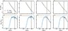 |
Fig. A.1. Evolution of M⋆ (top) and MBH (bottom) in the N-body simulations (blue, solid line) presented in Arca Sedda et al. (2024a) and in this work (orange dashed line). Different columns show the evolution of some representative N-body simulations. The two left-hand panels show the evolution of a GC with N = 3 × 10⁵ stars, while the two right-hand panels show the evolution of GCs with N = 1.2 × 10⁵ stars. The black vertical dashed line is the time of the GC core collapse. |
In the N-body models, the total BH mass within the half-mass radius initially increases because the most massive stars progressively give birth to BHs, and peaks at tcc. Subsequently, the total BH mass decreases because of dynamical ejections within the BH subsystem. For this comparison, we set the initial MBH to the value given by the N-body simulations at tcc, which ranges from 0.042 to 0.05. In our runs, we assume an initial BH mass fraction of 0.045.
A.5. Coupling between CLUSTERBH and FASTCLUSTER
In this section, we describe how we interface the two semi-analytic codes CLUSTERBH (Antonini & Gieles 2020) and FASTCLUSTER (Mapelli et al. 2021). First, we generate the GC masses and densities and calculate the time of core collapse (eq. A.3). We draw the 1g BBH masses, spins and orbital properties as described in Sect. 2.2.1. For each metallicity, we set in both FASTCLUSTER and CLUSTERBH the value of mBH to the mean BH mass in the MOBSE catalog.
We evolve the host GC until the time of core collapse, if BHs are not ejected by their natal kick. To ensure efficiency along with accuracy, we implemented a Runge-Kutta fourth order integrator and an adaptive time-step in CLUSTERBH. Specifically, we increase (reduce) the time-step by a factor of 2 (10) if the percentage change of the integrated quantities (M⋆, MBH or rhm) between two time-steps falls below 0.1% (exceeds 1%). After BBH formation, we integrate the GC mass, radius, density and velocity dispersion, along with the BBH eccentricity and semi-major axis (see eq. 16 in Mapelli et al. 2021). Since the evolution timescales of the BBH and the host GC generally differ by several orders of magnitude, we implement two separate adaptive time-step schemes for integrating the BBH hardening and the GC evolution, respectively.
We stop GC evolution if the BH is ejected from the cluster (e.g. as a consequence of three-body interactions or relativistic recoil) or when the integration reaches the Hubble time. If the GC evaporates, or no BHs are retained within the cluster, we continue the BBH evolution as an isolated binary, as described in Mapelli et al. (2021). Our implementation delivers an efficient integration of both the GC and the BBH properties, and enables us to evolve ∼3 × 10⁵ BBHs in GCs per day with a single core.
Appendix B: Impact of the initial GC mass and density on our results
The initial GC mass and density distributions we assumed in the main text (Sect. 2.1) match the observed properties of current Milky Way GCs (Harris et al. 2013; VandenBerg et al. 2013). However, GCs might have been more massive and denser at their formation time (e.g., Vesperini 1998). In the following, we estimate the impact of GC initial conditions on the BBH merger rate density by considering larger initial GC masses and densities. In particular, we assume that the initial median value of the GC mass (density) distribution is two (ten) times as large as the values considered in Sect. 2.1.
Figure B.1 shows that larger GC masses and densities have a mild impact on the primary BH mass. As expected, denser, and more massive clusters produce a higher BBH merger rate density, because of a higher BH retention fraction. In models B and C, the merger rate of low-mass BHs is enhanced, because supernova kicks are less efficient in ejecting them from more massive GCs. In contrast, the mass sampling presented in model A is only marginally affected by this effect, because only massive BHs tend to pair-up efficiently with this mass sampling.
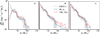 |
Fig. B.1. Primary BH mass merger rate density for models A (left), B (center), and C (right) in the Tidal evolutionary case. The GC masses and densities are initialized as described in Sect. 2.1, (M0, ρ0, blue solid line), and with mass (density) distributions that are shifted to larger values by a factor 2 (10, red dashed line). The black dashed line is the median value of the POWER LAW + PEAK model inferred from GWTC-3 (Abbott et al. 2023b). The gray shaded areas are the corresponding 90% credible intervals. |
The longer cluster lifetime and the shorter evolution timescales also enhance the production of hierarchical mergers. However, also in this case we find a minor contribution from ng ≥ 3 mergers at redshift z = 0, especially for the ng1g cases (models A and C).
Appendix C: Hierarchical BH mass function as a function of metallicity
Figure C.1 shows the primary BH mass distribution produced by BBH mergers at different metallicities. In model A, the main peak shifts with the maximum mass of first-generation BHs. Also, for each metallicity, this pairing function predicts a secondary peak due to hierarchical mergers at ∼2max(m1, 1g).
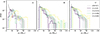 |
Fig. C.1. Probability distribution function of primary BH masses in GCs, for models A (left), B (center), and C (right) in the Tidal evolutionary case. We consider different progenitor metallicities: Z = 0.02 (purple solid line), Z = 0.016 (blue dotted line), Z = 0.006 (green dashed line), and Z = 0.002 (yellow dash-dotted line). The black dashed line is the median value of the POWER LAW + PEAK model inferred from GWTC-3 (Abbott et al. 2023b). The gray shaded areas are the corresponding 90% credible intervals. |
In models B and C, the main peak at 10 M⊙ is mainly due to BBH mergers at solar (Z = 0.02) and slightly subsolar metallicity (Z = 0.016), while lower metallicities extend the mass distribution toward larger masses. As discussed in Sect. 3.4, the relative contribution of different metallicities results in a variation of the BH primary mass distribution with redshift. In models B and C, primary BH masses m1 < 20 M⊙ become less and less common at z ≥ 2, because metal-rich progenitors (Z = 0.02, 0.016) also become less frequent at high redshift. In model A, the main peak of the primary BH mass shifts from ∼35 M⊙ to ∼50 M⊙ as a function of redshift, because metal-poor stars become more and more common at high redshift.
Appendix D: Bayesian hierarchical analysis
To compare our models against GW events in the third-GW transient catalog, we use a hierarchical Bayesian approach, as we already described in previous work (Bouffanais et al. 2019, 2021; Mapelli et al. 2022). Given a number Nobs of GW observations,  , described by an ensemble of parameters θ, the posterior distribution of the hyper-parameters λ associated with the models is described as an inhomogeneous Poisson distribution (Loredo 2004; Mandel et al. 2019):
 (D.1)
(D.1)
where θ are the GW parameters, Nλ is the number of events predicted by the astrophysical model, μλ is the predicted number of detections associated with the model and the GW detector, π(λ, Nλ) is the prior distribution on λ and Nλ, and ℒk({h}k|θ) is the likelihood of the kth detection. The predicted number of detections is given by μ(λ) = Nλ β(λ), where
 (D.2)
(D.2)
is the detection efficiency of the model. In eq. D.2, pdet(θ) is the probability of detecting a source with parameters θ and can be inferred by computing the optimal signal-to-noise ratio and comparing it to a detection threshold, as described, e.g., in Bouffanais et al. (2021).
The values for the event’s log-likelihood are derived from the posterior and prior samples released by the LVC, such that the integral in eq. D.1 is approximated with a Monte Carlo approach as
 (D.3)
(D.3)
where  is the ith posterior sample for the kth detection and
  is the total number of posterior samples for the kth detection. Both the model and prior distributions are estimated with Gaussian kernel density estimation. We further marginalise eq. D.1 over Nλ using a prior π(Nλ)∼1/Nλ (Fishbach et al. 2018), which yields the following expression:
 (D.4)
(D.4)
Based on the above calculations, we can estimate the mixing fraction as described in eq. 15. Figures D.1, D.2, D.3, and D.4 show the behavior of four selected models (isolated binaries, and models A, B, and C in the NoEv case, respectively) in the planes defined by the four parameters q, χeff, m1, and ℳchirp. In the histograms, we do not show all possible simulated BBHs, but rather only the detectable ones (i.e., with a S/N5 of above 8 assuming O3b sensitivity). From these figures, we see that BBHs from isolated binary systems tend to be associated with nearly aligned spins, while our dynamical models have a broader distribution of χeff, which is favored by the LVK data. This explains the large values of the mixing fraction fGC we obtain when we include the impact of χeff into our hierarchical Bayesian analysis. From these figures, we also see that isolated BBHs favor a strong peak at m1 ∼ 8 − 10 M⊙, similar to the main peak reported by the LVK Collaboration.
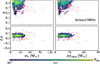 |
Fig. D.1. Two dimensional histograms of the detectable simulated BBHs in the isolated binary evolution model. The four panels show, from left to right and from top to bottom, q − m1, q − ℳchirp, χeff − m1, and χeff − ℳchirp. The red points are the data from Abbott et al. (2023b). We do not add error bars in order to avoid overcrowding the plot. |
All Tables
All Figures
|
Fig. 1. Distribution of first-generation primary (left) and secondary (right) masses of dynamical BBHs that are retained within the cluster (upper panels) and merge (lower panels). We show the distributions from the Dragon-II direct N-body simulations (Arca Sedda et al. 2024a, gray shaded area) and in FASTCLUSTER, produced by sampling A (blue dashed line) and B (red dot-dashed line). |
| In the text | |
|
Fig. 2. Primary BH mass distribution of BBH mergers for models A (left), B (center), and C (right) for the three evolutionary cases considered: NoEv (upper panels), Evol (middel panels), and Tidal (lower panels). Different colors correspond to different BH generations: 1g (blue), 2g (purple), 3g (salmon), and > 3g (yellow) BHs. Here, we show our models with Z = 0.0002 because they are representative of metal-poor GCs in the Galactic halo (Muratov & Gnedin 2010). |
| In the text | |
|
Fig. 3. Mass ratio distributions of BBH mergers for models A (left), B (center), and C (right) in the Tidal evolutionary case. Different colors correspond to different BH generations: 1g (blue), 2g (purple), 3g (salmon), and > 3g (yellow) BHs. Here, we show models with Z = 0.0002. |
| In the text | |
|
Fig. 4. Primary BH mass differential merger rate density in the Local Volume for models A (left), B (center), and C (right) for the NoEv (upper panels) and Tidal (lower panels) cases. We show the mass distribution resulting from 1g mergers (yellow dash-dotted line), 1g and 2g mergers (green dashed line), and from all BBH generations together (purple solid line). The black dashed line is the median value of the POWER LAW + PEAK model, as inferred from GWTC-3 (Abbott et al. 2023b). The gray shaded areas are the corresponding 90% credible intervals. In this and the following figures, the black line and shaded gray areas are shown only for a qualitative comparison, because our simulations do not assume the parametric models adopted by the LVK. |
| In the text | |
|
Fig. 5. Probability distribution function of primary BH masses at redshift z = 0 (black solid line), z = 1 (purple dotted line), z = 2 (salmon dashed line), and z = 3 (yellow dash-dotted line) for models A (left), B (center), and C (right) in the Tidal evolutionary case. In model B, the distribution extends to higher masses, but the plot is truncated at 150 M⊙ to improve the readability of the figure. The black dashed line is the median value of the POWER LAW + PEAK model, as inferred from GWTC-3 (Abbott et al. 2023b). The gray shaded areas are the corresponding 90% credible intervals. |
| In the text | |
|
Fig. 6. Primary BH mass (upper panels) and mass ratio (lower panels) differential merger rate density in the Local Volume for models A (left), B (center), and C (right) in the Tidal evolutionary case. We show the mass distribution resulting from isolated BBH mergers (blue solid line), 1g BBH mergers in GCs (yellow dash-dotted line), and all BBH mergers in GCs (including hierarchical mergers, salmon dashed line). The black dashed line is the median value of the POWER LAW + PEAK model inferred from GWTC-3 (Abbott et al. 2023b). The gray shaded areas are the corresponding 90% credible intervals: these are shown only for a qualitative comparison, because our simulations do not assume the parametric models adopted by the LVK. We refer to Appendix D for a quantitative analysis. |
| In the text | |
|
Fig. 7. Precessing (upper panels) and effective (lower panels) spin distribution of BBH mergers at redshift z = 0 for models A (left), B (center), and C (right) in the Tidal evolutionary case. We show the mass distribution resulting from isolated BBH mergers (blue solid line), 1g BBH mergers in GCs (yellow dash-dotted line), and BBH mergers in GCs, including hierarchical mergers (salmon dashed line). The black dashed line is the median value of the Gaussian spin model inferred from GWTC-3 (Abbott et al. 2023b). The gray shaded areas are the corresponding 90% credible intervals. |
| In the text | |
|
Fig. 8. Mixing fraction (fGC) probability distribution function. A mixing fraction fGC = 0 (fGC = 1) means that all BBHs are born from isolated binary systems (GCs). In the upper and lower panels, we and do not marginalize over the spin parameters χeff and χp in our analysis, respectively. All the models presented in this paper are shown with different colors, as described in the legend. |
| In the text | |
|
Fig. A.1. Evolution of M⋆ (top) and MBH (bottom) in the N-body simulations (blue, solid line) presented in Arca Sedda et al. (2024a) and in this work (orange dashed line). Different columns show the evolution of some representative N-body simulations. The two left-hand panels show the evolution of a GC with N = 3 × 10⁵ stars, while the two right-hand panels show the evolution of GCs with N = 1.2 × 10⁵ stars. The black vertical dashed line is the time of the GC core collapse. |
| In the text | |
|
Fig. B.1. Primary BH mass merger rate density for models A (left), B (center), and C (right) in the Tidal evolutionary case. The GC masses and densities are initialized as described in Sect. 2.1, (M0, ρ0, blue solid line), and with mass (density) distributions that are shifted to larger values by a factor 2 (10, red dashed line). The black dashed line is the median value of the POWER LAW + PEAK model inferred from GWTC-3 (Abbott et al. 2023b). The gray shaded areas are the corresponding 90% credible intervals. |
| In the text | |
|
Fig. C.1. Probability distribution function of primary BH masses in GCs, for models A (left), B (center), and C (right) in the Tidal evolutionary case. We consider different progenitor metallicities: Z = 0.02 (purple solid line), Z = 0.016 (blue dotted line), Z = 0.006 (green dashed line), and Z = 0.002 (yellow dash-dotted line). The black dashed line is the median value of the POWER LAW + PEAK model inferred from GWTC-3 (Abbott et al. 2023b). The gray shaded areas are the corresponding 90% credible intervals. |
| In the text | |
|
Fig. D.1. Two dimensional histograms of the detectable simulated BBHs in the isolated binary evolution model. The four panels show, from left to right and from top to bottom, q − m1, q − ℳchirp, χeff − m1, and χeff − ℳchirp. The red points are the data from Abbott et al. (2023b). We do not add error bars in order to avoid overcrowding the plot. |
| In the text | |
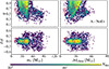 |
Fig. D.2. Same as Figure D.1 but for model A NoEv. |
| In the text | |
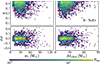 |
Fig. D.3. Same as Figure D.1 but for model B NoEv. |
| In the text | |
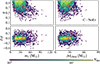 |
Fig. D.4. Same as Figure D.1 but for model C NoEv. |
| In the text | |
Current usage metrics show cumulative count of Article Views (full-text article views including HTML views, PDF and ePub downloads, according to the available data) and Abstracts Views on Vision4Press platform.
Data correspond to usage on the plateform after 2015. The current usage metrics is available 48-96 hours after online publication and is updated daily on week days.
Initial download of the metrics may take a while.