| Issue |
A&A
Volume 685, May 2024
|
|
|---|---|---|
| Article Number | A51 | |
| Number of page(s) | 20 | |
| Section | Galactic structure, stellar clusters and populations | |
| DOI | https://doi.org/10.1051/0004-6361/202348509 | |
| Published online | 03 May 2024 | |
Impact of gas hardening on the population properties of hierarchical black hole mergers in active galactic nucleus disks⋆
1
Institut für Theoretische Astrophysik, ZAH, Universität Heidelberg, Albert-Ueberle-Straße 2, 69120 Heidelberg, Germany
e-mail: mariapaolavaccaro@gmail.com; mapelli@uni-heidelberg.de
2
Physics and Astronomy Department Galileo Galilei, University of Padova, Vicolo dell’ Osservatorio 3, 35122 Padova, Italy
3
INFN – Padova, Via Marzolo 8, 35131 Padova, Italy
4
INAF – Osservatorio Astronomico di Padova, Vicolo dell’Osservatorio 5, 35122 Padova, Italy
5
Departamento de Ciencias Fisicas, Universidad Andres Bello, Fernandez Concha 700, Las Condes, Santiago, Chile
Received:
6
November
2023
Accepted:
31
January
2024
Hierarchical black hole (BH) mergers in active galactic nuclei (AGNs) are unique among formation channels of binary black holes (BBHs) because they are likely associated with electromagnetic counterparts and can efficiently lead to the mass growth of BHs. Here, we explore the impact of gas accretion and migration traps on the evolution of BBHs in AGNs. We have developed a new fast semi-analytic model, that allows us to explore the parameter space while capturing the main physical processes involved. We find that an effective exchange of energy and angular momentum between the BBH and the surrounding gas (i.e., gas hardening) during inspiral greatly enhances the efficiency of hierarchical mergers, leading to the formation of intermediate-mass BHs (up to 104 M⊙) and triggering spin alignment. Moreover, our models with efficient gas hardening show both an anticorrelation between the BBH mass ratio and the effective spin and a correlation between the primary BH mass and the effective spin. In contrast, if gas hardening is inefficient, the hierarchical merger chain is already truncated after the first two or three generations. We compare the BBH population in AGNs with other dynamical channels as well as isolated binary evolution.
Key words: black hole physics / gravitation / gravitational waves / stars: black holes / stars: kinematics and dynamics / galaxies: active / galaxies: nuclei
© The Authors 2024
 Open Access article, published by EDP Sciences, under the terms of the Creative Commons Attribution License (https://creativecommons.org/licenses/by/4.0), which permits unrestricted use, distribution, and reproduction in any medium, provided the original work is properly cited.
This article is published in open access under the Subscribe to Open model. Subscribe to A&A to support open access publication.
1. Introduction
The first direct detection of gravitational waves (GWs) in 2015 (Abbott et al. 2016) paved the ground for the study of binary black holes (BBHs). More than 90 GW event candidates have been detected to date, most of them associated with BBHs (Abbott et al. 2023a,b). A few BBH candidates, such as GW190521 (Abbott et al. 2020) and possibly GW190403_051519 and GW190426_190642 (Abbott et al. 2021, 2023a,b), stand out because they involve black holes (BHs) in the pair-instability mass gap, challenging traditional models of stellar evolution (Woosley et al. 2002; Woosley & Heger 2014, 2021; Belczynski et al. 2016; Spera & Mapelli 2017; Stevenson et al. 2019; O’Brien 2021; Siegel et al. 2022; Sabhahit et al. 2023; Umeda & Nagele 2024) and raising questions about their formation (Farmer et al. 2019, 2020; Mapelli et al. 2020; Belczynski 2020; Marchant & Moriya 2020; Costa et al. 2021; Farrell et al. 2021; Vink et al. 2021; Tanikawa et al. 2021, 2022; Dall’Amico et al. 2021; Banerjee 2022; Méndez et al. 2023).
Stellar dynamics provides some of the most straightforward channels to explain the birth of such oversized BHs, via star–star collisions (Di Carlo et al. 2019, 2020; Kremer et al. 2020; Renzo et al. 2020; Torniamenti et al. 2022; Costa et al. 2022; Ballone et al. 2023) or repeated mergers of stellar-origin BHs (Miller & Hamilton 2002; Fishbach et al. 2017; Gerosa & Berti 2017; Rodriguez et al. 2019; Doctor et al. 2020; Kimball et al. 2020; Flitter et al. 2021; see, e.g., Mapelli 2021 for a review). The latter process, often called hierarchical mergers, takes place only in dense star clusters, where merger remnants can be retained inside the system (e.g., Antonini et al. 2019; Fragione & Silk 2020) and pair up again with other single BHs via dynamical encounters (e.g., Heggie 1975; Portegies Zwart & McMillan 2000). In order to constrain the origin of the observed BBH mergers, it is important to characterize the hierarchical merger process in different environments, such as young star clusters (YSCs, e.g., Ziosi et al. 2014; Mapelli 2016; Banerjee 2017a,b, 2020; Di Carlo et al. 2020; Kumamoto et al. 2019, 2020), globular clusters (GCs, e.g., Downing et al. 2010; Rodriguez et al. 2015, 2016, 2018; Askar et al. 2017; Fragione & Kocsis 2018; Zevin et al. 2019; Antonini & Gieles 2020; Antonini et al. 2023), nuclear star clusters (NSCs, e.g., O’Leary et al. 2009; Miller & Lauburg 2009; Antonini & Rasio 2016; Petrovich & Antonini 2017; Leigh et al. 2017; Arca Sedda & Gualandris 2018; Arca Sedda 2020; Atallah et al. 2023; Chattopadhyay et al. 2023), and active galactic nuclei (AGNs, e.g., McKernan et al. 2012, 2020, 2022; Bartos et al. 2017; Stone et al. 2017; Yang et al. 2019a; Secunda et al. 2020; Tagawa et al. 2020b,a, 2022, 2023; Ford & McKernan 2022).
In AGNs, a central supermassive black hole (SMBH) is surrounded by a dense gaseous accretion disk. AGNs can appear as extremely luminous objects called quasars, but also as Seyfert galaxies, radio galaxies, or blazars, depending on their luminosity and our viewing angle (see Netzer 2015 for a review of the unification scheme and its controversy). Stars and stellar-sized BHs orbiting the SMBH are subject to gas torques, which can bend their orbits, aligning them with the disk. This is expected to lead to a large overdensity of BHs with similar orbits in small areas of the disk called migration traps (McKernan et al. 2012; Bellovary et al. 2016), where BHs can pair up efficiently via gas capture (DeLaurentiis et al. 2023; Li et al. 2023; Rowan et al. 2023, 2024; Whitehead et al. 2023). Therefore, AGNs are potential factories of BBH mergers with masses in the pair-instability mass gap and above (Yang et al. 2019a; Tagawa et al. 2020a,b).
This channel has attracted great interest because GW signals from mergers could be accompanied by some electromagnetic emission (Bartos et al. 2017; Tagawa et al. 2023), possibly anticipated by a neutrino detection (Zhu 2024; Zhou & Wang 2023). To explore this possibility, electromagnetic follow-up observations have been carried out for several GW events, but so far all associations with BBH mergers remain controversial (Greiner et al. 2016; Coughlin et al. 2020; Calderón Bustillo et al. 2021).
Several studies have investigated the possibility that the high-mass BBH merger event GW190521 is associated with an AGN disk (Tagawa et al. 2021; Samsing et al. 2022) because of its large mass, high spin (Abbott et al. 2020), and claimed electromagnetic counterpart (Graham et al. 2020; Calderón Bustillo et al. 2021; Morton et al. 2023). Yang et al. (2019a) explored the AGN scenario for another high-mass BBH, GW170729, for which there is evidence of nonzero effective and precessing spins. Some authors, such as Gayathri et al. (2021) and Ford & McKernan (2022), have predicted that a sizeable fraction of the observed BBH mergers (∼20% up to 80%) may originate in AGNs. However, according to an analysis based on the sky localization of GW signals, the fraction of detected BBH mergers that originated in bright AGNs (L ≥ 1046 erg s−1) cannot be higher than 17% (Veronesi et al. 2023).
Binary BH pair-up in AGNs can happen either in the migration traps or at other locations in the disk (Wang et al. 2021) collectively referred to as ‘the bulk’. McKernan et al. (2020) find that, although more than 50% of mergers happen in the bulk, hierarchical mergers are only efficient in migration traps. Moreover, Tagawa et al. (2020b) find that BBHs assembled in the bulk via gas capture migrate toward the migration trap while hardening.
The complex physics of BBHs in AGN disks has been extensively explored in the literature, with studies accounting for the effects of binary–single interactions (Stone et al. 2017; Leigh et al. 2017) and gas torques (using models borrowed from protoplanetary physics; e.g., McKernan et al. 2012; Bartos et al. 2017; Yang et al. 2019a,b; Secunda et al. 2020; or hydrodynamical simulations; e.g., Li et al. 2023; Kaaz et al. 2023; Rowan et al. 2023, 2024; Whitehead et al. 2023). For example, Ishibashi & Gröbner (2020) explore the effects of energy and angular momentum exchange between the BBH and the surrounding gas. In particular, they assume that the BBH evolves surrounded by a circumbinary disk, which induces orbital decay and increases its orbital eccentricity (i.e., gas hardening).
We studied hierarchical BBH mergers in the migration traps of AGN disks and compared our results to mergers in YSCs, GCs, and NSCs (Mapelli et al. 2021, 2022). Specifically, we tested the impact of gas hardening (GH) on the BBH merger population in AGNs (Ishibashi & Gröbner 2020). We find that the hierarchical merger process is pronouncedly more efficient when accounting for gas hardening.
We have developed a new semi-analytic code for the simulation of hierarchical mergers in AGNs. It is effective at exploring the parameter space, and it models the relevant physical processes much faster than an N-body or hydrodynamical code. The new code is publicly available within the FASTCLUSTER software environment1 (Mapelli et al. 2021, 2022).
2. Methods
2.1. AGN disk model
We assumed the AGN disk to be as described by Sirko & Goodman (2003, hereafter, SG). These authors introduce a hydro-dynamical model for a geometrically thin and optically thick disk with steady-state accretion of 0.1 ṀEdd onto the central SMBH. Gas turbulence is assumed to be the cause of disk viscosity, characterized by the viscosity coefficient α ∈ [0, 1]. This model neglects any effects due to magnetic fields and general relativity. The physical parameters of the disk are functions of the mass of the SMBH MSMBH, the distance R from the SMBH, and the viscosity parameter α. We slightly simplified the radial dependence of the SG model for numerical ease and re-scaled their functions to allow for different MSMBH and α parameters, as shown in Fig. 1. The resulting expressions for the gas surface density, Σgas, the disk aspect ratio, h = H/R (defined as the ratio between the height of the disk, H(R), and its radius, R), and the sound speed, cs, are the following:
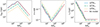 |
Fig. 1. Surface density, Σgas, aspect ratio, h and sound speed, cs, profiles as a function of the scale distance, R/Rg. Dashed maroon lines represent the SG model for a disk with viscosity α = 0.01 around a 108 M⊙ SMBH. Solid blue lines show our broken power-law best fit to the SG model for α = 0.01 and MSMBH = 108 M⊙. The dash-dotted green and dotted orange lines show our fits for a 107 M⊙ and a 106 M⊙ SMBH, respectively (both with α = 0.01). |
In the above equations, we define the gravitational radius as Rg = GMSMBH/c2, where G is the gravity constant and c the speed of light.
The viscosity coefficient α is a free parameter. We assumed it to be constant over the whole extension of the disk and to have a constant value independent of the other physical properties of the disk. The assumed value is α = 0.1 which is consistent with observations (King et al. 2007).
Migration traps are locations in the disk where migration stalls and BHs pile up. Bellovary et al. (2016) find that migration traps are located where the slope of the gas surface density profile changes sign from positive to negative (i.e. at local maxima). In a SG disk there are two local maxima in the gas surface density and therefore two migration traps: an inner trap at ≈100 Rg and an outer one at ≈1300 Rg.
We see in Fig. 1 that the inner migration trap coincides with a local maximum in the density profile of the original SG model, while the outer migration trap corresponds to a global maximum. For simplicity, we ignored the local overdensity in the disk at 102 Rg and we only assumed the existence of the outer migration trap. We thus defined the trap radius as Rtrap = 103.1 Rg, although its location and existence may be affected by other effects (e.g. Grishin et al. 2024; Pan & Yang 2021 more details in Sect. 4.4).
The disk is assumed to have radial extension between the innermost stable circular orbit (ISCO) radius for a nonrotating BH, which we call Rmin = 6 Rg in this context, and an outer radius Rmax = 0.1 pc(MSMBH/106 M⊙)1/2, beyond which the disk’s self-gravity becomes important (Goodman 2003; Yang et al. 2019b). For R > Rmax, the disk is expected to fragment and experience star formation. Energetic feedback from the newly formed stars may keep the disk vertically supported (Sirko & Goodman 2003), but the outcome of viscous interactions with the BHs in this region of the disk is highly uncertain, so we conservatively neglected it. Moreover, we neglected the contribution of stars formed in AGN disks, which are expected to be massive and whose compact remnants might also become GW sources (Cantiello et al. 2021; Wang et al. 2023).
We assumed a non-spinning SMBH. We randomly generated the SMBH mass from the observational distribution derived by Greene & Ho (2007) in the Local Universe, which is a Gaussian distribution with mean ⟨log MSMBH/M⊙⟩ = 6.576 ± 0.591.
A mass-accretion episode onto a SMBH lasts for a finite amount of time, which we refer to as the AGN disk lifetime. The lifetime of AGN disks is subject to large uncertainty: different estimates span several orders of magnitude in the range of 10−2 − 103 Myr (Khrykin et al. 2021). Also, it is not clear whether accretion onto SMBHs happens continuously over a given time span, or episodically through many cycles of efficient accretion. Here, we used the estimate by Khrykin et al. (2021), based on observations of quasars’ proximity effect. They find that the quasar lifetime τ is distributed according to a Gaussian distribution with mean ⟨log τ/Myr ⟩ = 0.22 ± 0.80. We randomly extracted the lifetime for AGN disks in our model from this distribution.
There are other models for stable AGN accretion disks, with notably different features compared to the one we adopt here. For example, the model by Thompson et al. (2005) differs from the SG model in both density and aspect ratio (McKernan et al. 2022). We will explore the impact of different disk models in a follow-up study.
2.2. Nuclear star cluster (NSC)
Supermassive black holes and NSCs commonly inhabit galactic spheroids with stellar masses ranging from 108 M⊙ to 1011 M⊙ (Graham & Spitler 2009). For MSMBH ≤ 5 × 10⁷ M⊙, the mass of the SMBH and that of the NSC scale as
For MSMBH > 5 × 10⁷ M⊙, the SMBH generally does not coexist with a NSC and we set MNSC = 0.
The effective radius of a NSC mildly correlates to its mass (Neumayer et al. 2020). The best-fit relation between the mass of the NSC and its effective radius is
To account for the spread in the data, we sampled log(rh/pc) from a Gaussian distribution with the mean centered on the corresponding value determined by Eq. (5) and width σ = 0.1 (0.2) for MNSC < 106 M⊙ (≥106 M⊙) so that most of the data fell under the ±2σ dispersion.
We approximated the spatial distribution of stars in the NSC with a Plummer (1911) model, with mass
where R is the distance from the SMBH, and aPL = rh/(1.3 pc) is the scale parameter for the Plummer model.
The mass fraction of stellar-origin BHs in the AGN disk fBH is sampled from a Gaussian with mean 0.04 and standard deviation 0.01 to account for mass segregation in the NSC (Bartos et al. 2017). The number of BHs in the AGN disk and their cumulative mass are thus given by the following equations:
where MNSC(Rmax) is defined in Eq. (6), the mean stellar-origin BH mass ⟨mBH⟩ is computed from data obtained from the population synthesis simulation code SEVN2 (Iorio et al. 2023) at solar metallicity (Appendix A), the distance Rmax is the outer radius of the disk (Sect. 2.1), the factor 1/2 accounts for prograde orbiters3 only, and the mean stellar mass ⟨m*⟩ ≃ 1 M⊙ is computed using a Kroupa (2001) initial mass function.
The parameter ftrap is the ratio between the number of BHs that are able to reach the migration trap on a timescale shorter than the disk lifetime τ and the total number of BHs that interact with the disk: this study focuses on BBH pair-ups in the migration trap, and therefore we are not interested in any BHs situated outside of that location. An operational definition of ftrap is given in Sect. 2.3.3.
We assumed the velocity dispersion of stars to scale with the SMBH mass as (Merritt & Ferrarese 2001)
However, it has been shown (e.g. Scott & Graham 2013; Sahu et al. 2019; Graham 2022) that this result depends on the morphology of galaxies included in the sample. For example, Sahu et al. (2019) find an exponent of ∼1/6 and show that it is caused by the combined contribution of Sérsic (i.e., following the Sérsic 1963 brightness profile) and core-Sérsic (i.e., centrally depleted) galaxies following two different MSMBH − σ relations with exponents (5.75±0.34)−1 and (8.64±1.10)−1, respectively.
2.3. First-generation (1g) BHs
We randomly drew first-generation (1g, i.e., stellar-origin) BH masses mBH from a catalog obtained with the population synthesis code SEVN (Spera & Mapelli 2017; Spera et al. 2019; Mapelli et al. 2020; Iorio et al. 2023). SEVN relies on up-to-date stellar tracks (Bressan et al. 2012; Costa et al. 2019; Nguyen et al. 2022) and models the formation of compact objects by taking into account electron-capture (Giacobbo & Mapelli 2019), core-collapse (Iorio et al. 2023) and pair-instability supernovae (Mapelli et al. 2020). In particular, here we used the rapid core-collapse supernova model from Fryer et al. (2012), which enforces the existence of a mass gap between the maximum neutron star mass and the minimum BH mass (Özel et al. 2010). We used the fiducial model from Iorio et al. (2023) and considered single stellar evolution only, as described in Appendix A. We assumed metallicity Z = 0.02 (i.e., approximately solar), which matches the typical metallicity at the center of massive galaxies in the Local Universe (Gallazzi et al. 2008).
We randomly drew an initial radial position for each BH. The radial extension of the accretion disk is small compared to the typical dimension of a NSC, so we neglected mass segregation on this scale and considered the numerical density of objects at radii R < Rmax to be uniform in radius: R ∼ 𝒰(Rmin,Rmax).
We drew the dimensionless spin magnitude, χ, from a Maxwellian distribution with one-dimensional root-mean-square σχ = 0.1, truncated at χ = 1. We chose σχ = 0.1 because it is reminiscent of the spins inferred from the third GW transient catalog (GWTC-3, Abbott et al. 2023b). This assumption does not take into account that the BBH population in GWTC-3 likely comes from multiple formation channels, including the AGN disk scenario. Current data are not sufficiently informative to differentiate between formation channels. We set the primary spin tilt as in Appendix B.
2.3.1. Gas capture
After setting up the properties of 1g BHs, we followed their evolution in the disk. When NSC objects orbit around the central SMBH, their orbits can cross the disk and gather some of the disk gas, subjecting them to strong gas drag. This is expected to dampen both the inclination i and the eccentricity e of their orbit (Cresswell et al. 2007). Therefore, after a sufficient number of laps, these objects will have circular orbits embedded in the disk. This process is called gas capture or orbital damping.
The gas accretion and subsequent gas drag are significant only for prograde orbiters. Hence, we neglected any variation in the orbits of retrograde orbiters.
We defined the inclination damping timescale, tdamp, for a BH of mass, mBH, on an initial orbit of semimajor axis4, A, around a SMBH of mass, MSMBH, as (Wang et al. 2024)
where Σgas(A) is the surface density of the gas. In this model, we neglect the mass increase due to gas accretion. Hence, during the orbital evolution, mBH is a constant quantity.
2.3.2. Migration
Once a BH is embedded in the disk, it exchanges angular momentum with the surrounding gas and is subject to gas torques. Torques can be both positive or negative, leading to outward or inward migration, respectively. Similar to what happens to planet seeds in protoplanetary disks, migration can happen in two different ways called Type I and Type II.
Small to medium-mass objects are subject to Type I migration, meaning that they change their radial position in the disk without significantly perturbing the density distribution of the disk itself. For a BH of mass mBH on a circular orbit with radius R, this happens on the timescale (Lyra et al. 2010; McKernan et al. 2012; Baruteau et al. 2014)
where h is the aspect ratio of the disk and Ω is the Keplerian angular velocity around the SMBH. Differently from Eq. (9), here we are considering a radius, R, rather than a semimajor axis, A, because gas capture happens necessarily before migration5, so the orbits have already been circularized when migration sets in.
In our disk model (Fig. 1), torques are positive in the inner region of the disk, where the slope of the surface density is positive, and they are negative in the outer region, where the slope of the surface density is negative (Bellovary et al. 2016). Therefore, Type I migration is directed outward in the inner disk and inward in the outer disk. At the location where the torques change sign, called a migration trap, migration will stall leading to a large accumulation of objects. Hence, after a timescale tmigr, I (Eq. (10)), the migrating object will be in the migration trap.
Larger objects, on the other hand, can open gaps in the disk. This happens because the motion of a massive object exerts an intense tidal perturbation on the disk, which effectively pushes material away from the orbit’s trail (Bryden et al. 1999). This is called Type II migration. An object of mass mBH can open a gap in the disk if (McKernan et al. 2014)
where q = mBH/MSMBH is the mass ratio with respect to the central SMBH, α is the viscosity parameter, and h = h(R) is the aspect ratio of the disk at radius R.
If an object opens a gap in the disk, assuming that no gas can cross the gap, its migration follows the viscous evolution of the disk’s gas. Hence, the timescale for Type II migration is the timescale for the viscous evolution of the disk (McKernan et al. 2012):
However, pressure forces in the disk push to close the gap. So, even if an object is massive enough to open a gap, such a gap can stay open against pressure forces only if (Bryden et al. 1999; McKernan et al. 2014)

Type II migrators typically have high mass: taking as fiducial values α = 0.1 and h = 0.02, Eqs. (11) and (13) entail mBH ≳ 0.1 MSMBH. They are bound to their radial location in the disk and can only move with the disk on its viscous timescale. Hence, they will never reach the migration trap. Moreover, the gaps they create will prevent some Type I migrators from reaching the trap: they will intercept inward-moving migrators if they are located at a radius greater than the trap’s, or they will intercept outward moving migrators if the opposite is true. These intercepted BHs can potentially pair up and merge with the Type II migrator, although their merger would not be assisted by GH. However, we expect such a massive BH in an AGN disk only in two cases: a high-generation hierarchical BH or the central BH of a dwarf galaxy dragged into the AGN disk after a galaxy–galaxy merger (e.g., Di Matteo et al. 2008). Describing galaxy mergers is out of the scope of this paper, while a high-generation hierarchical BH can form only in the late stages of the disk’s lifetime. We can assume that by that point most of the BHs have already migrated in the migration trap, and we can neglect any further pair-up event with a Type II migrator.
Therefore, in our model we consider the onset of Type II migration to be one of the processes that can halt hierarchical mergers. Moreover, the presence of gaps has noteworthy consequences on disk structure. Nevertheless, we bluntly neglect any evolution of the disk density profile.
2.3.3. Pair-up
Depending on the physical properties of the AGN (such as viscosity, gas density, aspect ratio, and SMBH mass), gas capture and migration can happen on short timescales. When these processes are efficient, they can lead to a large abundance of BHs in the narrow region of the migration trap. Also, all BHs in the migration traps are on similar orbits (prograde and quasi-Keplerian), so their relative velocities of encounter are small. Under such conditions, it is easy for two BHs to become gravitationally bound in a binary. Therefore, efficient damping and migration lead to efficient binary pair-up.
In this work, we assume that the pair-up of a primary and secondary BH is immediate as soon as the primary reaches the migration trap. This assumption is fully justified by the efficiency of dynamical friction in the migration trap (see Qian et al. 2024 and Sect. 4). The pairing timescale of a BBH is therefore

where tin is the formation time of the primary BH since the time of formation of the disk.
We considered each BBH to be in a circular orbit in the migration trap at a radius Rtrap (Sect. 2.1). We computed the fraction, ftrap, of BHs that reach the migration trap by counting the number of 1g BHs for which tpair < τ, where τ is the disk lifetime, and dividing it by the total number, N, of simulated first-generation BHs. We used this parameter for the computation of the maximum mass that can be accreted by a single BH, as in Eq. (7).
2.3.4. BBH properties
We determined the secondary BH mass as in Appendix C, and we set the secondary BH spin in the same way as for the primary BH. We set the secondary BH spin tilt as in Appendix B. We assigned the initial semimajor axis, a, of the binary sampling from a distribution p(a) ∝ a9/2 (Binney & Tremaine 2008; Tagawa et al. 2020b) for a ∈ [amin,amax], where amin = 1 R⊙ and amax is equal to the Hill radius, computed as
where m1 and m2 are the primary and secondary BH mass, respectively. We set the initial eccentricity e following a thermal distribution p(e)∝2e for e between 0 and 1 (Jeans 1919).
According to the Heggie (1975) law, a binary can survive in a star cluster only if it is hard, meaning that its binding energy is greater than the average kinetic energy of a field star
where a is the semimajor axis of the binary, ⟨m*⟩ is the average mass of a star in the NSC, and σ is the three-dimensional velocity dispersion. Hence, we dynamically evolveed hard binaries only.
2.4. Orbital evolution and merger
Once the binary is in the migration trap, we set R = Rtrap and update the quantities in Eqs. (1)–(3) accordingly. The semimajor axis, a, and eccentricity, e, of a binary with component masses m1 and m2, embedded in the disk, evolve due to GH, irrespective of whether the binary is prograde or retrograde, as (Ishibashi & Gröbner 2020)
![$$ \begin{aligned} \ \dot{e}_\mathrm{gas}&= \frac{12\pi \,\alpha \,c_\mathrm{s} ^2 \,\Sigma _\mathrm{gas} \,(1-e^2)^{1/2}\,(1+e)^2\,[ 1-(1-e^2)^{1/2}]}{\mu \, \Omega _{\rm b}\,e}, \end{aligned} $$](/articles/aa/full_html/2024/05/aa48509-23/aa48509-23-eq18.gif)
where μ = m1m2/(m1 + m2) is the reduced mass and  is the Keplerian orbital frequency.
The binary also hardens due to the effect of GW emission, which will govern the evolution at small semimajor axes. The evolution of the semimajor axis, ȧGW, and eccentricity, ėGW, due to GW hardening proceeds as in Peters (1964).
The interaction with other objects also contributes to the hardening of hard binaries according to Heggie (1975). We neglected the hardening effect due to three-body interactions because they typically occur on a timescale longer than that of GH (Leigh et al. 2017, see discussion in Sect. 4.3). The overall evolution of the binary is thus described by

The equations for GH (Eqs. (17) and (18)) are valid under the assumption that gravitational torques from the binary act axisymmetrically upon the disk so that they clear a cavity in the surrounding gas distribution, which remains circular throughout its inspiral. This is an idealized model since cavities in AGN disks can become eccentric (MacFadyen & Milosavljević 2008; Cimerman & Rafikov 2024) and can lead the orbital separation to grow in time (Miranda et al. 2016). Hence, we considered an “optimistic” model in which the evolution is given by Eq. (19) (hereafter, the GH model), and a “pessimistic” model in which we neglect GH and only consider the effect of GW emission (hereafter, the no-GH model). In both the optimistic and pessimistic cases, we integrated the hardening equations using the Euler method and an adaptive timestep (Mapelli et al. 2021).
We refer to the delay time between the pair-up and the merger as tdel. If tpair + tdel is longer than the lifetime of the disk, the disk has evaporated before the binary could merge. In this case, the BBH keeps hardening due to GW emission only.
We assumed that the BBH merges when its members cross the ISCO radius of a non-spinning BH with mass equal to the total mass of the binary system, rISCO = 6 G (m1 + m2)/c2, with a tolerance of 0.1 rISCO. This happens on a merger timescale

We modeled the mass and spin of the merger remnant using fitting formulas from numerical relativity, as described by Jiménez-Forteza et al. (2017). At birth, merger remnants receive a relativistic kick vkick because of the transfer of linear momentum caused by asymmetries in GW emission. We used the model of Maggiore (2018, Eq. (14.202)) for the magnitude and direction of the kick velocity, vkick.
The relativistic kick vkick pushes the merger remnant out of the migration trap. We computed the new velocity as vfin = vKepl(Rtrap)+vkick, where the Keplerian velocity in the migration trap is computed accounting for the mass of the SMBH MSMBH and the inner part of the NSC MNSC, while neglecting the mass of the gas disk:
The final semimajor axis Afin of the remnant orbit, computed by means of simple orbital transfer calculations (Hohmann 1960), is
![$$ \begin{aligned} A_\mathrm{fin} =\frac{G M_\mathrm{TOT} (R_\mathrm{trap} )}{v_\mathrm{fin} ^2} \; \left[\frac{R_\mathrm{trap} \,v_\mathrm{fin} ^2 / G M_\mathrm{TOT} (R_\mathrm{trap} )}{2 - R_\mathrm{trap} \,v_\mathrm{fin} ^2 / G M_\mathrm{TOT} (R_\mathrm{trap} )} \right]. \end{aligned} $$](/articles/aa/full_html/2024/05/aa48509-23/aa48509-23-eq23.gif)
The quantities in Eqs. (1)–(3) were updated accordingly.
As a safety check, we ensured that the new orbital semimajor axis, Afin, is smaller than the maximum radius of the disk, Rmax, meaning that the remnant can experience damping and become embedded in the disk. Otherwise, we did not consider the remnant for future generations.
2.5. Nth-generation (Ng) BHs
A seed BH can only go through a finite number of hierarchical mergers before it comes across one of the following scenarios:
-
The disk has evaporated. Therefore, damping, migration, and any other effects due to gas torques stop. We evaluated this by checking if, at generation N, the merger timescale,
 , is shorter than the disk lifetime, τ. In our formalism, we defined the merger timescale of a Ng BH as
 ![$ t_\mathrm{merg}^{(N)} = t_\mathrm{in}^{(N)} + [{ t_\mathrm{damp} + t_\mathrm{migr,\,I} +t_\mathrm{del}}]^{(N)} $](/articles/aa/full_html/2024/05/aa48509-23/aa48509-23-eq25.gif) , where
, where  is the evolutionary time of the previous generations.
 -
The relativistic kick received at merger is so strong that the remnant is ejected from the AGN. We computed the escape velocity considering only the gravitational potential of the SMBH and the inner NSC, while neglecting the mass of the gaseous disk, as
Then we computed the final velocity after kick vfin = vin + vkick and ensured that it is smaller than the escape velocity, vesc. We also ensured that the merger remnant is on a disk-crossing orbit by comparing its semimajor axis, Afin, with the outermost disk radius, Rmax.
-
The number of BHs in the NSC is finite. Therefore, the mass that can be accreted is limited and the BH may not find any more companions to pair up with. We kept track of the mass accreted by a single BH, which is the sum of its initial mass, m1, and of the masses of all the secondaries,
 , it pairs up and merges with
where the index N represents the generation number. We ensure that the BH does not accrete more mass than what is available in the inner NSC in the form of other BHs, namely
 , where
  is obtained as in Eq. (7).
 -
The BH is so massive that it opens a gap in the disk and can only move from its radial location due to Type II migration. We checked whether both conditions in Eqs. (11) and (13) are respected. For typical values of viscosity and aspect ratio, these conditions entail mBH ≳ 10−1MSMBH.
If any of conditions (1)–(4) was met, we did not consider the merger remnant for future generations. We followed the evolution of Nth generation BHs with a procedure similar to the one outlined for first-generation BHs. In hierarchical mergers, the remnant of an (N − 1)th-generation merger acts as the primary BH for the Nth-generation. So, the primary mass and spin are simply set as the remnant mass and spin of the previous generation, computed according to Jiménez-Forteza et al. (2017). Similarly, the initial position of the primary component of the Nth-generation BBH is set as the position of the merger remnant of the previous generation, set in Eq. (22). This value is used to compute the pairing time tpair = tdamp + tmigr, I + tin, where for Nth generations  . The migration and pair-up physics are the same as described for the first generation.
We modeled the secondary component of each Nth-generation BBH as described in Appendix C. We define an Nth-generation (Ng) BH to be the result of the repeated merger of N stellar-origin BHs. For instance, an Ng BH can be the result of either an Mg − 1g merger (where M + 1 = N) or an Mg − Lg merger (where M + L = N, L > 1). We kept iterating the same procedure until the considered BH met at least one of requirements (1)–(4).
2.6. Cosmic evolution
We modeled the cosmic evolution of AGNs using data from the ILLUSTRISTNG100, a magneto-hydrodynamical cosmological simulation adopting a cubic box of size (110.7 Mpc)3 with a resolution of roughly (6 Kpc)3 (see Pillepich et al. 2018 and Springel et al. 2018 for further details).
We calibrated the AGN density distribution nAGN(z) in the ILLUSTRISTNG data by choosing a threshold in the mass accretion rate such that the value at redshift zero, nAGN(0), is compatible with the observational value of ∼6 × 10⁻⁶ Mpc−3 obtained from a sample of X-ray-selected AGNs (Buchner et al. 2015). As displayed in Fig. 2, we find that setting this threshold to a fifth of the Eddington mass accretion rate, namely ṀSMBH ≥ 0.2 ṀEdd, provides an appropriate normalization. We employed nAGN(z) to compute the BBH merger rate properties in various redshift bins as explained in Appendix D.
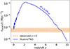 |
Fig. 2. Number density of active SMBHs per unit comoving volume, nAGN(z), in the ILLUSTRISTNG100 simulation (solid blue lines) vs. the observational values at redshift zero for unobscured (hydrogen column density NH ≲ 1023 cm−2) high-luminosity (L ≥ 1043.2 erg s−1) AGNs. |
The SMBH mass distribution is expected to evolve as a function of redshift (Weinberger et al. 2018). Nevertheless, since the mass evolution cannot be constrained by current data, we used the observational distribution from Greene & Ho (2007) at every redshift for simplicity.
2.7. Description of runs
We considered two different models for the AGN channel: with and without GH (hereafter, GH and no-GH). We ran N = 105 realizations of our two models, each with different SMBH mass and AGN lifetime randomly extracted as described at the end of Sect. 2.1. In each run, we simulated all the BHs that reach the migration trap within the AGN disk lifetime.
Furthermore, we simulated four other channels (isolated, YSC, GC, and NSC) with the same code (FASTCLUSTER; Mapelli et al. 2021, 2022) and using the same underlying initial conditions, such as the stellar evolution model determining the 1g BHs mass distribution (Appendix A). This allowed us to filter out any bias that might arise by using different numerical codes for different environments: the differences we see are not due to the numerical approach adopted but to intrinsic differences among channels. We performed a Bayesian analysis to determine the AGN mixing fraction as described in Appendix E.
3. Results
3.1. Impact of gas hardening
We find that the efficiency of the hierarchical merger process is significantly higher in the presence of GH: in our GH model, seed BHs can go through up to roughly 500 merger episodes, whereas in the no-GH case the hierarchical chain usually stops after a few generations (Fig. 3). In the GH (no-GH) model, the hierarchical merger chain stops because of the condition on timescales, maximum mass, Type II migration, or ejection in the 58.7% (81.6%), 27.1% (18.0%), 13.6% (0%), and 0.6% (0.4%) of simulations, respectively.
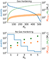 |
Fig. 3. Number of mergers and characteristic masses at each merger generation. The blue histogram and the left-hand y-axis show the number of BBH merger events for each hierarchical merger generation, Ng. The orange (green) shaded area and the upper right-hand y-axis show the 25%–75% percentile of the chirp mass (primary mass) for merging BBHs of each generation. The orange (green) dots and lower right-hand y-axis show the average chirp mass (primary mass) for merging BBHs of each generation. |
Figure 4 shows the main properties of dynamically assembled BBHs in our AGN simulations. We display only BBHs that merge within a Hubble time. In both models, hierarchical mergers in the migration trap are successful in producing BBHs with primary mass in the pair-instability mass gap and above, but there is a major difference between the GH and no-GH scenarios: the primary BH mass extends only up to 300 M⊙ in the no-GH scenario, while it reaches ≈5 × 10³ M⊙ in the GH scenario, because GH dramatically increases the efficiency of hierarchical mergers. Hence, the GH mechanism produces a recognizable feature in the high-mass end (m1 ≳ 100 M⊙) of the mass spectrum. This is caused by the stark difference in delay timescales (Fig. 4f) due to the different GH prescriptions: in the GH scenario, the relative distribution has a pronounced peak between 1 yr and 1 Myr, which in the no-GH case is absent. Information on other relevant timescales is illustrated in Sect. 3.4. Secondary BHs can also have masses in the pair-instability mass gap but only up to a few times 102 M⊙ in the GH scenario, as the AGN channel tends to favor mergers with low mass ratio (Fig. 4b).
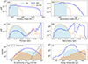 |
Fig. 4. Main properties of dynamical BBH mergers in our GH and no-GH AGN models. The unfilled solid blue (dashed orange) histogram shows BBHs in the GH (no-GH) AGN scenario. The filled blue (orange) histogram shows the 1g BBHs in the GH (no-GH) AGN scenario. If 1g BHs in the no-GH scenario are identical to the GH scenario, they are not shown. Panels (a) and (b): probability density function (pdf) of the primary and secondary BH mass (m1 and m2). Panels (c) and (d): primary and secondary spin magnitudes (χ1 and χ2). Panel (e): orbital BBH eccentricity e(10 Hz) when the GW frequency is fGW = 10 Hz. In gray we show the thermal distribution p(e) = 2e for comparison. Panel (f): timescales of delay time, tdel, between the BBH pair-up and the merger. |
The GH model has a sharp peak in the distribution of the primary spin magnitude at χ1 = 1 as well as a peak in the distribution of the secondary spin magnitude at χ2 ≃ 0.9 associated with high-generation mergers (Fig. 4c,d). Both models GH and no-GH also have a peak at χ1 ≈ 0.75 (also χ2 ≈ 0.75 for the GH case), corresponding to the second generation.
The distribution of spin-tilt angles is influenced by GH, as shown in Fig. 5 and explained in Appendix B. In the no-GH scenario, the spin tilts θ1, 2 are isotropically distributed with respect to the orbital angular momentum L. Instead, in the presence of GH, χ1, χ2, and L are all preferentially aligned with each other. The distribution of the secondary spin tilt θ2 is slightly wider than the primary’s spin tilt, because of a cumulative effect: the misalignment between χ2 and L is set keeping into account the misalignment between χ1 and L (see Appendix B).
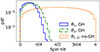 |
Fig. 5. Probability density function (pdf) of spin tilt angles θ1 and θ2. The blue (green) histogram shows the primary (secondary) spin tilt in the GH scenario. The unfilled orange histogram shows the primary and secondary tilts in the no-GH scenario. The first generation is not shown separately in this plot because the distributions are identical at each generation. |
Both scenarios preferentially produce BBHs with low eccentricity when6 the GW frequency is 10Hz. Nevertheless, they can produce BBHs with eccentricity e ≥ 10−2 (Fig. 4e), which is potentially detectable by the LIGO-Virgo-KAGRA (LVK) interferometers (Romero-Shaw et al. 2021). In our GH model, there are two processes at play: GH pumps the eccentricity (Eq. (18)), whereas GW emission damps it (Peters 1964). Hence, the GH scenario is more likely to produce BBHs with eccentricity in the range e ∈ [10−5, 10−2] for fGW = 10 Hz than the no-GH one. In a more accurate model, we should also include the effect of three-body scatterings (Samsing et al. 2022) and tidal forces exerted by the SMBH (Rom et al. 2024), both of which pump BBH eccentricity.
Figure 6 shows the relation between the BBH mass m1 + m2 and mass ratio m2/m1 in our models, compared to GW data (Abbott et al. 2023a,b). The AGN channel tends to favor mergers with low mass ratio (Appendix C). This effect is particularly important for high primary BH masses m1 ≳ 102 M⊙ when accounting for GH.
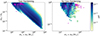 |
Fig. 6. Probability density function (pdf) of the binary mass and mass ratio for all BBH mergers in our simulations (blue color palette). We do not apply any selection effects to our simulations. Left-hand (right-hand) panels: GH (non-GH) scenario. The magenta dots show the median values of the parameters for LVK BBH merger event candidates with pastro > 0.9 from GWTC-3 (Abbott et al. 2023a,b). We do not include error bars for readability purposes. |
The effective spin distribution in the GH model (Fig. 7) peaks at χeff ∼ 1, corresponding to maximum alignment, and shows lower peaks at χeff ≃ 0.2 and χeff ≃ 0.5. From Fig. 8, we see that 1g mergers populate the peak at χeff ≃ 0.2, 2g mergers create a peak at χeff ≃ 0.5, while third- and higher-generation BBHs contribute the main peak at χeff ≃ 1. The precession spin distribution, instead, has no sharp features in this scenario.
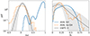 |
Fig. 7. Effective (left) and precession spin (right) probability density functions (pdf) GH (solid blue lines) and no-GH (dashed orange lines) model. We do not apply any selection effects to our simulations. Solid black lines show the posterior distribution inferred from LVK data, after applying a parametric-model description of the intrinsic BBH population with hierarchical Bayesian inference (Abbott et al. 2023b). |
In the no-GH scenario, the orbital angular momentum is isotropically oriented with respect to the AGN disk (Appendix B). This produces a bell-shaped effective spin distribution centered on χeff = 0 with half-width at half-maximum HWHM ≃ 0.3 and a precession spin distribution that peaks at χp ≃ 0.2 and χp ≃ 0.75 (Fig. 7). As the BBH generation increases, so does the magnitude of its BH spins, making the corresponding effective spin distribution progressively wider as shown in Fig. 8. The peaks at χp ≃ 0.2 and 0.7 are populated mostly by 1g and 2g mergers, respectively, whereas the tail at χp > 0.8 results from higher-generation mergers.
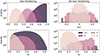 |
Fig. 8. Effective and precession spin distributions for the GH (left-hand panels) and no-GH (right-hand panels) models, where the shade represents different hierarchical merger generations. The lightest hue refers to the first generation (stellar-origin BHs), while the darkest hue refers to generations higher than the third. |
3.2. Anticorrelation between q and χeff
Figure 9 shows the relationship of the effective spin with primary mass and mass ratio of BBH mergers in our simulations. In the GH scenario, there is a clear correlation between effective spin and BBH mass, as well as a clear anticorrelation between effective spin χeff and mass ratio q. This is a possible explanation for the anticorrelation between χeff and q found in the LVK data (Callister et al. 2021; Santini et al. 2023). If this anticorrelation stems from hierarchical mergers in the GH regime, our simulations suggest that it should extend to lower mass ratios and higher effective spins than currently observed by LIGO and Virgo.
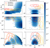 |
Fig. 9. Effective spin correlations with relevant BBH parameters. The top row shows the probability density distribution for the primary BH mass, m1, and the effective spin, χeff, compared with posterior contour plots at credibility levels 50% and 90% of LVK BBH merger events GW190521 (dash-dotted red line, Abbott et al. 2020) and GW170729 (solid orange line, Abbott et al. 2023b), and LVK transient event GW190403_051519 (dashed yellow line, Abbott et al. 2021). The central (bottom) row has the same legend as the first row, but shows the mass ratio, q = m2/m1, (precession spin, χp) and the effective spin, χeff. |
The anticorrelation is particularly noticeable for χeff ≳ 0.4 because all higher-generation mergers display the following features: high mass, small mass ratio, and high effective spin. In the no-GH model, both the spin alignment and the hierarchical merger process are suppressed; so there is no clear correlation between the aforementioned quantities.
3.3. Comparison with other channels
Figure 10 compares the main properties of BBH mergers in five different formation channels, namely AGN disks, NSCs, GCs, YSCs, and isolated binary evolution (iso). The simulations for NSCs, GCs, YSCs, and iso adopt the same setup as model B of Mapelli et al. (2022), and use as initial conditions catalogs of BH masses derived with SEVN (Iorio et al. 2023), for consistency with the catalogs of the AGN channel. We provide more details about NSC, GC, YSC, and iso simulations in Appendix A.
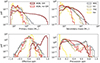 |
Fig. 10. Probability density distribution (pdf) of the primary and secondary BH masses, m1, 2, the effective spin, χeff, and the precession spin, χp, in the five channels modeled with FASTCLUSTER: active galactic nuclei (AGNs) with GH (solid dark red line) or with no-GH (dashed bright red line), NSCs (dark gray line), GCs (light gray line), YSCs (dark gold line), and isolated binary evolution (light gold line). |
All dynamical formation channels can produce BBH mergers with masses and spin magnitudes higher than the isolated channel. The no-GH AGN disk scenario resembles most closely the results of the other dynamical channels, whereas the GH AGN disk channel is completely different from the others.
The population of dynamical channels appears as follows: the mass distributions show one or two peaks at a few tens of solar masses and a tail that extends up to a few hundred solar masses; the effective spin distribution is symmetric, peaks at χeff = 0, and has a half width at half maximum of ∼0.5 (∼0.3 for the YSC channel); and the precession spin distribution has two peaks, at χp ≃ 0.2 and χp ≃ 0.7. This contrasts with the isolated channel population, which features a primary (secondary) BH mass distribution that does not extend any higher than 50 M⊙ (40 M⊙).
The primary BH mass distribution for the GH AGN channel, instead, extends up to ∼5 × 10³ M⊙. The effective spin distribution has two sharp peaks at χeff ≃ 0.2 and χeff ≃ 1, as well as a minor peak at χeff ≃ 0.5, whereas the precession spin distribution has no evident peaks.
We computed the mixing fractions, fmix, for our five channels, as described in Appendix E. To derive fmix, we marginalized over the merger rate density, to avoid this extremely uncertain quantity affecting our results. As shown in Fig. 11, the NSC and YSC channels are associated with larger median mixing fractions than the other channels. This happens because, in our models, the NSC channel can account for the peak at low BH mass (m1 ≈ 10 M⊙) found in the LVK data, while the YSC channel contributes mostly to the high-mass peak at ∼35 M⊙ (Abbott et al. 2023b). In fact, in our model, the YSC scenario produces larger median BBH masses than the NSC scenario, because the escape velocity from YSCs is much lower, preventing the low-mass BHs from merging in YSCs (they are ejected by supernova kicks, see the discussion in Mapelli et al. 2021). The isolated channel also produces BBH mergers with a peak of the primary BH mass at ∼10 M⊙, but has too little support for zero and negative values of χeff with respect to the observed ones. The mass and spin properties of the GC scenario are intermediate between YSCs and NSCs.
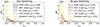 |
Fig. 11. Mixing fractions obtained with our five-channel analysis (see Appendix E). The left-hand (right-hand) plot shows the GH (no-GH) AGN channel model. |
There is a small difference between the mixing-fraction distribution of the GH and no-GH scenarios because this analysis only considers detectable events: the most massive BHs of the GH population (which are the main difference with respect to the no-GH model) have no impact on fmix. Overall, our results confirm that the current LVK sample of BBH mergers is too small and the uncertainties on theoretical models are too large to draw an informative mixing-fraction analysis with five channels (see Sect. 3.4 of Mapelli et al. 2022).
3.4. Timescales
Figure 12 shows the distribution of all relevant timescales with and without GH. Both the damping time tdamp and the migration time tmigr, I span a large range, which is representative of the large range in SMBH mass and initial position R. The damping timescale for the first hierarchical merger generation has a flat distribution in the range 10−4 − 102 Myr, while the migration timescale ranges between 10−2 and 103 Myr. In the GH scenario, tdamp and tmigr, I display additional peaks for subsequent generations at 10−5 Myr and 10−2 Myr, respectively. The delay timescale tdel spans a large range of values, because of the large range encompassed in BH masses and initial BBH semimajor axes. In the GH scenario, it has a pronounced peak at ∼1 yr, whereas in the no-GH case it is typically as large as the Hubble timescale (∼14 Gyr). Indeed, the longest timescale in the no-GH scenario is the delay timescale. In the GH scenario, instead, the evolution is overall governed by the migration timescale.
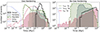 |
Fig. 12. Relevant timescales in our model. The black line shows the overall merger timescale, tmerg. The dash-dotted green line shows the gas capture timescale, tdamp, (the shaded green histogram shows tdamp for 1g BBHs only). The dotted navy line shoiws the Type I migration timescale, tmigr, I, (the shaded navy histogram shows tmigr, I for 1g BBHs only). The dashed pink line shows the delay timescale, tdel, between the pair-up and the merger (the shaded pink histogram shows tdel for 1g BBHs only). The light blue line shows the gas dynamical friction timescale, τ0, related to BBH pairing (Qian et al. 2024). |
We also display the timescale for gas dynamical friction τ0, responsible for BBH pair-up, which we discuss in Sect. 4.2. It is typically on the order of 10−13 Myr and can be as short as 10−20 Myr for the disk parameters in our model; hence, it is negligible compared to other timescales at play.
4. Discussion
4.1. Outlook for ET and LISA
We studied the evolution of hierarchical mergers in the migration traps of AGN disks and explored the role of GH. Our models, especially the GH scenario, predict the formation of merger events with higher mass than is detectable by current ground-based detectors. Indeed, the frequency emitted by a BBH depends on its mass and steadily increases during its inspiral. The frequency of the ISCO is equal to (Maggiore 2008)
Figure 13 shows the probability distribution function of the maximum emitted frequency by AGN BBHs. The LVK interferometers are only sensitive in the frequency range from a few tens of hertz up to ∼1 KHz (Abbott et al. 2023a). Hence, only a fraction of our predicted merger events in the GH scenario are observable with existing detectors.
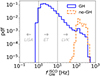 |
Fig. 13. Predictions for the Einstein Telescope (ET) and the Laser Interferometer Space Antenna (LISA). The solid blue (dashed orange) histogram shows the probability density functions (pdf) for ISCO emitted GW frequencies in the GH (no-GH) scenario. The gray lines show the approximate detectable frequencies of LVK detectors, ET, and LISA. |
The next generation ground-based interferometers, the Einstein Telescope (ET) and Cosmic Explorer (Punturo et al. 2010; Maggiore et al. 2020; Evans et al. 2021; Branchesi et al. 2023), and space-borne interferometers Laser Interferometer Space Antenna (LISA), Deci-hertz Interferometer GW Observatory (DECIGO) and TianQin (Amaro Seoane et al. 2013, 2017; Luo et al. 2016; Kawamura et al. 2019) will be able to detect GW signals with lower frequency than currently possible. For example, the frequency range of the ET and Cosmic Explorer (≈1 − 104 Hz) has substantial overlap with the GW frequency of BBH mergers from the GH AGN channel, with the exception of the very high-mass tail. LISA will instead be sensitive to frequencies lower than ∼1 Hz (Robson et al. 2019), so it would be able to detect the highest-mass end of the synthetic mergers predicted by our GH AGN model. We will explore detectability by ET and LISA in detail in a follow-up work.
4.2. BBH pair-up
In our model, we assume that the pairing of a primary and a secondary BH is immediate as soon as the primary reaches the migration trap. A realistic model for BBH pair-up in AGN disks should keep into account GW two-body capture, three-body encounters, and gas dissipation. Whitehead et al. (2023) run hydro-dynamical simulations of close encounters between pairs of BHs embedded in the gaseous disk and find that dissipation by gas gravitation is not always efficient for the formation of bound BBHs. Specifically, they find that it is usually an effective mechanism for BBH formation for gas densities ρg in the range ![$ -4.5 \lesssim \log[{\rho_\mathrm{g}R_\mathrm{H}^{3}/({m_1+m_2})}] \lesssim -2.5 $](/articles/aa/full_html/2024/05/aa48509-23/aa48509-23-eq34.gif) , where RH is the Hill radius of the BBH. In our simulations, we typically have
, where RH is the Hill radius of the BBH. In our simulations, we typically have ![$ \log[{\rho_\mathrm{g}R_\mathrm{H}^{3}]/({m_1+m_2}}) \simeq -6 $](/articles/aa/full_html/2024/05/aa48509-23/aa48509-23-eq35.gif) for our BBHs because the high gas density in the migration trap is compensated for by small Hill radii due to the proximity to the SMBH. Hence, gas dissipation is expected to be inefficient.
for our BBHs because the high gas density in the migration trap is compensated for by small Hill radii due to the proximity to the SMBH. Hence, gas dissipation is expected to be inefficient.
On the other hand, in their recent N-body simulations, Qian et al. (2024) find that BBH formation from two BHs on similar orbits embedded in the disk is efficient for Ω τ0 ≲ 10, where Ω is the Keplerian angular velocity of the BHs and

is the dynamical friction timescale (Ostriker 1999), which, as shown in Qian et al. (2024), is linearly related to the timescale of BBH pair-up. In our model typically Ω τ0 ∼ 10−4 − 10−3 due to the high gas density ρg in the migration trap, which justifies our assumption.
Moreover, we expect a high number density nBH of BHs in the migration trap due to efficient migration. This may further aid BBH pair-up because the timescales for two-body and three-body captures scale respectively as  (Quinlan & Shapiro 1990) and
  (Fragione & Silk 2020). In future work, we will further explore the process that leads to BBH pair-up, accounting for these additional effects.
In this work we neglect BBH formation in the bulk (i.e., outside of the migration trap), which is expected to be efficient due to the high number of Type I migrators embedded in the disk (e.g. Tagawa et al. 2020a,b). Interestingly, gas-assisted bulk-assembled BBHs migrate toward the migration trap while hardening (Tagawa et al. 2020b, Fig. 8). Hence, some binaries may merge in the migration trap even if they were assembled in the bulk.
4.3. Three-body encounters
We neglect three-body interactions and their effects on BH scattering and BBH hardening. We make this approximation because of the dearth of semi-analytical models for these interactions: in the literature, there are some works (e.g., Coleman Miller & Lauburg 2009; Fragione & Silk 2020) that assume an isotropic distribution of velocities and are appropriate for spherical star clusters. In a Keplerian disk geometry, the distribution of velocities is much different and these models are not appropriate (McKernan et al. 2022). Nevertheless, a hard binary hardens via binary–single encounters (Heggie 1975), and this has a twofold effect: the inspiral of BBHs is accelerated via three-body effects, and the third intruding body receives a recoil kick that may prevent it from reaching the migration trap. Also, binary-single interactions are expected to increase the eccentricity of all BBHs to e(10 Hz) ≥ 10−4 and potentially flip the orientation of the BBH orbital angular momentum, leaving key signatures in the effective spin distribution (Samsing et al. 2022). Additionally, Rowan et al. (2023) show that the initial eccentricity of BBHs formed in AGN disks is high, which is not well modeled by our assumption of a thermal distribution (Jeans 1919).
Tagawa et al. (2020b) simulated the evolution of the compact object population in AGN disks using a one-dimensional N-body simulation combined with a semi-analytical model for the formation, disruption, and evolution of binaries. They include the effects of three-body interactions and employ a Thompson et al. (2005) disk model rather than the SG model that we use. Nevertheless, comparing our Fig. 6 with Tagawa et al. (2020b, Fig. 12a), we can point out that the output from our fiducial model is compatible with the output from theirs. This suggests that three-body effects have a relatively minor impact on the population of merging BBHs.
Leigh et al. (2017) find that the approximate encounter timescale between a BH in the migration trap and an intruder is a fraction of the Type I migration timescale (Eq. (10)) of an object of mass m* starting its migration from the outer skirts of the disk, namely
![$$ \begin{aligned} t_\mathrm{enc} \simeq \frac{t_\mathrm {migr,\,I} \left(R_\mathrm{max} \right)}{N_*} = \frac{1}{N_*} \left[ \frac{M_{\rm SMBH}^2\, h^2\left(R_\mathrm{max} \right)}{m_*\, \Sigma _\mathrm{gas} \left(R_\mathrm{max} \right) \,R_\mathrm{max} ^2\, \Omega _*}\right] , \end{aligned} $$](/articles/aa/full_html/2024/05/aa48509-23/aa48509-23-eq39.gif)
where N* is the number of Type I migrators in the disk.
Assuming m* = 1 M⊙ and N* = 100, we find that the encounter timescale is typically larger than the delay timescale in the GH scenario (Fig. 14). This justifies our disregarding of three-body effects in this scenario. Nevertheless, they should be included in the no-GH model.
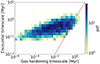 |
Fig. 14. Delay timescale, tdel, in the GH model compared against the three-body encounter timescale, tenc, estimated as in Leigh et al. (2017). The red line is tdel = tenc. |
This implies that Heggie’s law (employed in Eq. (16)) may not be valid in the GH case, as even soft binaries may be hardened considerably on a timescale shorter than the one on three-body interactions. We find that forming soft BBHs in our model is an extremely rare event (fewer than 1 in 10 000 BBHs), so including them in our computation would not have affected the results significantly.
Furthermore, efficient damping, migration, and BBH pair-up in AGN disks are expected to give rise to a high concentration of BBHs in migration traps. Hence, we should take into account the effect of binary-binary interactions. Such encounters are expected to efficiently ionize one of the binaries involved and lead to the formation of a stable triple (Marín Pina & Gieles 2024).
4.4. Position of migration traps
The position of migration traps is highly uncertain: it strongly depends on the disk model and the migration prescription used. For instance, Pan & Yang (2021) compute Type I migration torques in the locally isothermal approximation as well as torques due to winds and to the gravitational interaction with the SMBH for three different disk models. In their approximation, no disk model develops migration traps. Moreover, they find that in the inner part of the disk (R ≲ 102Rg) Type I migration torques are always overpowered by the other effects, which prompt embedded BHs to eventually merge with the SMBH. This justifies our assumption that we can neglect the inner migration trap for the SG model (Sect. 2.1), but it implies that we somewhat overestimate the number of Type I migrators.
In their recent work, Grishin et al. (2024) account for both Type I migration, caused by the gravitational perturbation of embedded BHs in the disk, and thermal migration, caused by the thermal response of the disk to the small and overdense accretion disks surrounding embedded BHs. They find that the resulting migration trap position is at much larger distances than previously identified by considering Type I migration only.
In our fiducial model, we followed the prescription by Bellovary et al. (2016) and identified the position of the migration trap as Rtrap = 1324 Rg, whereas Grishin et al. (2024) find that the updated position of the migration trap is typically larger Rtrap = 103 − 106 Rg, and has a steep dependence on the SMBH mass as

for MSMBH ≲ 108 M⊙. Hence, for a typical SMBH of mass 106 M⊙, the migration trap is at ∼105 Rg.
Migration is also affected by the additional thermal torque, which reduces the migration timescale by a factor of
where tmigr, I is defined as in Eq. (10).
Figure 15 shows a comparison between the results of our fiducial model and the results we obtain assuming the position of migration traps and the migration timescales predicted by Grishin et al. (2024). We find that the hierarchical merger process is suppressed when including a treatment for thermal torques, as only a handful of seed BHs reach the second generation in our simulations. This happens because the gaseous disk is significantly thicker and more diluted in the outer area of the disk where the new migration trap is located (see Sect. 2.1). Therefore, as the migration timescale is proportional to h3 and  , the migration process is much slower in this scenario. Moreover, even when BHs successfully reach the migration trap, the delay timescale ends up being too long because of the low gas surface density.
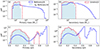 |
Fig. 15. Main properties of dynamical BBH mergers with two different models for the migration timescale and the location of migration traps. The solid blue line shows the fiducial GH model. The dashed red line shows the results of runs where we used the model by Grishin et al. (2024) for both the migration timescale and the location of the migration trap. Filled light blue histograms refer to 1g mergers in the fiducial model. Panels (a) and (b): primary and secondary BH masses. Panels (c) and (d): primary and secondary BH spin magnitudes. |
4.5. General caveats
In our model, we disregard dynamical interactions with the SMBH and gravitational perturbations caused by intermediate-mass BHs. For example, Deme et al. (2020) show that the presence of intermediate-mass BHs in the disk may enhance the ionization of BBHs and consequently decrease the merger rate.
Moreover, in Sect. 2.3.1 we assumed that eccentricity and inclination of a BH orbit are damped on similar timescales due to gas torques. Wang et al. (2024, Fig. 4) show that this is not always accurate: if the initial orbit is highly eccentric (e ≳ 0.9), the eccentricity-damping timescale can be up to five times longer than the inclination-damping one. A BH on a gas-embedded eccentric orbit (i ∼ 0, e ≳ h) would be subject to spin-down (McKernan & Ford 2023), which would leave an imprint on the expected spin distribution.
Finally, we ignored the evolution of AGN disks in time. This can happen slowly over the AGN lifetime as BHs are embedded in the disk (Tagawa et al. 2022) and gas is accreted by the SMBH. The efficiency of all dynamical processes strongly depends on disk density and aspect ratio. If these quantities evolve over time, the resulting BBH population will be affected as well.
4.6. GW190521 and other transient events
It has previously been suggested that the transient events GW170729 and GW190521 could have originated in AGN disks (Yang et al. 2019a; Tagawa et al. 2021; Samsing et al. 2022; Graham et al. 2020; Morton et al. 2023). In particular, Yang et al. (2019a) found that it is five times more likely for GW170729 to arise from hierarchical mergers in AGNs than assuming that all events in the GWTC-1 catalog (Abbott et al. 2019) arise from the same channel, whereas Morton et al. (2023) show that the association between GW190521 and the AGN flare ZTF19abanrhr (Graham et al. 2020) is highly preferred over the lack of association, suggesting that the GW transient event was generated in an AGN.
We compare the posterior contours for the primary mass and effective spins of such events with the output of our AGN simulations, as shown in Fig. 9. We also include the posterior contour of the transient event GW190403_051519, although it has a low S/N of  and a low probability of having an astrophysical origin, pastro = 0.61 (Abbott et al. 2021).
We find that the contours of GW170729 have some overlap with both the GH and the no-GH AGN models, and thus might be compatible with an origin in an AGN environment. In contrast, GW190521 has no significant overlap with our models in the χeff − m1 space, and negligible overlap with our no-GH model in the χeff − χp space. Indeed, the posterior probability distribution of GW190521 shows moderate support for high precession spin and low effective spin, suggesting that its BH spin vectors are large but misaligned. In contrast, in our GH model, we predict that they should be aligned for a BBH of primary mass ∼100 M⊙. This does not rule out the hypothesis of an AGN origin for GW190521, as we might speculate that the BBH may have been perturbed by three-body encounters, which we do not account for in our GH model (Appendix B). This would alter the orientation of the orbital angular momentum and decrease the effective spin, as well as increase the BBH eccentricity (Samsing et al. 2022).
Finally, the posterior contours of GW190403_051519 significantly overlap with our GH AGN model. However, this event candidate has a high false alarm rate and may not have astrophysical origin (Abbott et al. 2021).
5. Summary
We explored the formation of BBH mergers in AGNs employing a new semi-analytical model. our key findings are as follows:
-
The presence of GH significantly increases the efficiency of hierarchical mergers in AGN disks, allowing seed BHs to go through up to 500 merger episodes. This leads to the formation of BBHs with high masses (up to a few thousand solar masses) and low mass ratios (q ≃ 10−2).
-
In contrast, if GH is not efficient, the hierarchical merger chain is truncated after a few generations, leaving a BBH population with no components more massive than ∼102 M⊙.
-
The distribution of spin tilt angles is influenced by GH. There is a preferential alignment of spins in the GH scenario and isotropic distribution in the no-GH scenario. Hence, GH leads to distinct features in the effective spin distributions: a main peak on χeff ≃ 1 corresponding to maximum alignment and smaller peaks at χeff ≃ 0.2 and χeff ≃ 0.5.
-
In the GH scenario, we find an anticorrelation between q and χeff that might even extend to lower values of q and higher values of χeff than currently observed by LVK.
-
Comparison with other formation channels shows that AGN-driven mergers in the GH scenario result in higher primary BH masses and higher effective spins.
In summary, we find that efficient GH in AGN disks enhances the formation of BBH mergers with high primary masses and low mass ratios, and leads to a strong preference for χeff ≈ 1. Given the high masses of BHs, next-generation ground-based detectors such as the ET are an ideal test bed for such unique features.
FASTCLUSTER is an open-source code available at https://gitlab.com/micmap/fastcluster_open
The latest public version of SEVN can be downloaded from this repository: https://gitlab.com/sevncodes/sevn
Here we only refer to BBH mergers with ISCO frequency in the LVK detectability range,  . See Sect. 4.1 for more details.
Acknowledgments
We thank the anonymous referee for their constructive and insightful comments that improved this manuscript. MM, MPV, CP, and ST acknowledge financial support from the European Research Council for the ERC Consolidator grant DEMOBLACK, under contract no. 770017. MPV and MM acknowledge financial support from the German Excellence Strategy via the Heidelberg Cluster of Excellence (EXC 2181 – 390900948) STRUCTURES. MD acknowledges financial support from the Cariparo Foundation under grant 55440. We thank Tamara Bogdanović, Barry McKernan, Dominika Wylezalek, Jenny Greene, Carolin “Lina” Kimmig, Ralf Klessen, Gastón Javier Escobar, Stefano Rinaldi, Giorgio Mentasti, Jacopo Tissino, Imre Bartos, Bence Kocsis, K.E. Saavik Ford, and Hiromichi Tagawa for their useful input. We thank Dylan Nelson for granting us access to the ILLUSTRISTNG JupyterLab workspace.
References
- Abbott, B. P., Abbott, R., Abbott, T. D., et al. 2016, Phys. Rev. Lett., 116, 061102 [Google Scholar]
- Abbott, B. P., et al. (LIGO Scientific Collaboration and Virgo Collaboration) 2019, Phys. Rev. X, 9, 031040 [Google Scholar]
- Abbott, R., Abbott, T. D., Abraham, S., et al. 2020, Phys. Rev. Lett., 125, 101102 [Google Scholar]
- Abbott, R., Abbott, T. D., Acernese, F., et al. 2021, ArXiv e-prints [arXiv:2108.01045] [Google Scholar]
- Abbott, R., Abbott, T. D., Acernese, F., et al. 2023a, Phys. Rev. X, 13, 041039 [Google Scholar]
- Abbott, R., Abbott, T. D., Acernese, F., et al. 2023b, Phys. Rev. X, 13, 011048 [NASA ADS] [Google Scholar]
- Amaro Seoane, P., Aoudia, S., Audley, H., et al. 2013, ArXiv e-prints [arXiv:1305.5720] [Google Scholar]
- Amaro Seoane, P., Audley, H., Babak, S., et al. 2017, ArXiv e-prints [arXiv:1702.00786] [Google Scholar]
- Antonini, F., & Gieles, M. 2020, MNRAS, 492, 2936 [CrossRef] [Google Scholar]
- Antonini, F., & Rasio, F. A. 2016, ApJ, 831, 187 [Google Scholar]
- Antonini, F., Gieles, M., & Gualandris, A. 2019, MNRAS, 486, 5008 [NASA ADS] [CrossRef] [Google Scholar]
- Antonini, F., Gieles, M., Dosopoulou, F., & Chattopadhyay, D. 2023, MNRAS, 522, 466 [NASA ADS] [CrossRef] [Google Scholar]
- Arca Sedda, M. 2020, ApJ, 891, 47 [Google Scholar]
- Arca Sedda, M., & Gualandris, A. 2018, MNRAS, 477, 4423 [NASA ADS] [CrossRef] [Google Scholar]
- Askar, A., Szkudlarek, M., Gondek-Rosińska, D., Giersz, M., & Bulik, T. 2017, MNRAS, 464, L36 [CrossRef] [Google Scholar]
- Atallah, D., Trani, A. A., Kremer, K., et al. 2023, MNRAS, 523, 4227 [NASA ADS] [CrossRef] [Google Scholar]
- Ballone, A., Costa, G., Mapelli, M., et al. 2023, MNRAS, 519, 5191 [NASA ADS] [CrossRef] [Google Scholar]
- Banerjee, S. 2017a, MNRAS, 467, 524 [NASA ADS] [Google Scholar]
- Banerjee, S. 2017b, MNRAS, 473, 909 [Google Scholar]
- Banerjee, S. 2020, MNRAS, 500, 3002 [CrossRef] [Google Scholar]
- Banerjee, S. 2022, A&A, 665, A20 [NASA ADS] [CrossRef] [EDP Sciences] [Google Scholar]
- Bartos, I., Kocsis, B., Haiman, Z., & Márka, S. 2017, ApJ, 835, 165 [Google Scholar]
- Baruteau, C., Crida, A., Paardekooper, S. J., et al. 2014, Protostars and Planets VI, 667 [Google Scholar]
- Belczynski, K. 2020, ApJ, 905, L15 [Google Scholar]
- Belczynski, K., Heger, A., Gladysz, W., et al. 2016, A&A, 594, A97 [NASA ADS] [CrossRef] [EDP Sciences] [Google Scholar]
- Bellovary, J. M., Low, M. M., McKernan, B., & Saavik Ford, K. E. 2016, ApJ, 819, L17 [NASA ADS] [CrossRef] [Google Scholar]
- Binney, J., & Tremaine, S. 2008, Galactic Dynamics: Second Edition (Priceton University Press) [Google Scholar]
- Bogdanović, T., Reynolds, C. S., & Coleman Miller, M. 2007, ApJ, 661, L147 [CrossRef] [Google Scholar]
- Bouffanais, Y., Mapelli, M., Santoliquido, F., et al. 2021, MNRAS, 507, 5224 [NASA ADS] [CrossRef] [Google Scholar]
- Branchesi, M., Maggiore, M., Alonso, D., et al. 2023, JCAP, 2023, 068 [CrossRef] [Google Scholar]
- Bressan, A., Marigo, P., Girardi, L., et al. 2012, MNRAS, 427, 127 [NASA ADS] [CrossRef] [Google Scholar]
- Bryden, G., Chen, X., Lin, D. N. C., Nelson, R. P., & Papaloizou, J. C. B. 1999, ApJ, 514, 344 [CrossRef] [Google Scholar]
- Buchner, J., Georgakakis, A., Nandra, K., et al. 2015, ApJ, 802, 89 [Google Scholar]
- Calderón Bustillo, J., Leong, S. H. W., Chandra, K., McKernan, B., & Ford, K. E. S. 2021, ArXiv e-prints [arXiv:2112.12481] [Google Scholar]
- Callister, T. A., Haster, C.-J., Ng, K. K. Y., Vitale, S., & Farr, W. M. 2021, ApJ, 922, L5 [NASA ADS] [CrossRef] [Google Scholar]
- Cantiello, M., Jermyn, A. S., & Lin, D. N. C. 2021, ApJ, 910, 94 [NASA ADS] [CrossRef] [Google Scholar]
- Chattopadhyay, D., Stegmann, J., Antonini, F., Barber, J., & Romero-Shaw, I. M. 2023, MNRAS, 526, 4908 [NASA ADS] [CrossRef] [Google Scholar]
- Chen, Y.-X., & Lin, D. N. C. 2023, MNRAS, 522, 319 [NASA ADS] [CrossRef] [Google Scholar]
- Cimerman, N. P., & Rafikov, R. R. 2024, MNRAS, 528, 2358 [NASA ADS] [CrossRef] [Google Scholar]
- Coleman Miller, M., & Lauburg, V. M. 2009, ApJ, 692, 917 [NASA ADS] [CrossRef] [Google Scholar]
- Costa, G., Girardi, L., Bressan, A., et al. 2019, MNRAS, 485, 4641 [NASA ADS] [CrossRef] [Google Scholar]
- Costa, G., Bressan, A., Mapelli, M., et al. 2021, MNRAS, 501, 4514 [NASA ADS] [CrossRef] [Google Scholar]
- Costa, G., Ballone, A., Mapelli, M., & Bressan, A. 2022, MNRAS, 516, 1072 [NASA ADS] [CrossRef] [Google Scholar]
- Coughlin, M. W., Dietrich, T., Antier, S., et al. 2020, MNRAS, 497, 1181 [NASA ADS] [CrossRef] [Google Scholar]
- Cresswell, P., Dirksen, G., Kley, W., & Nelson, R. P. 2007, A&A, 473, 329 [NASA ADS] [CrossRef] [EDP Sciences] [Google Scholar]
- Dall’Amico, M., Mapelli, M., Di Carlo, U. N., et al. 2021, MNRAS, 508, 3045 [CrossRef] [Google Scholar]
- DeLaurentiis, S., Epstein-Martin, M., & Haiman, Z. 2023, MNRAS, 523, 1126 [NASA ADS] [CrossRef] [Google Scholar]
- Deme, B., Meiron, Y., & Kocsis, B. 2020, ApJ, 892, 130 [NASA ADS] [CrossRef] [Google Scholar]
- Di Carlo, U. N., Giacobbo, N., Mapelli, M., et al. 2019, MNRAS, 487, 2947 [NASA ADS] [CrossRef] [Google Scholar]
- Di Carlo, U. N., Mapelli, M., Giacobbo, N., et al. 2020, MNRAS, 498, 495 [NASA ADS] [CrossRef] [Google Scholar]
- Di Matteo, T., Colberg, J., Springel, V., Hernquist, L., & Sijacki, D. 2008, ApJ, 676, 33 [NASA ADS] [CrossRef] [Google Scholar]
- Doctor, Z., Wysocki, D., O’Shaughnessy, R., Holz, D. E., & Farr, B. 2020, ApJ, 893, 35 [NASA ADS] [CrossRef] [Google Scholar]
- Downing, J. M. B., Benacquista, M. J., Giersz, M., & Spurzem, R. 2010, MNRAS, 407, 1946 [NASA ADS] [CrossRef] [Google Scholar]
- Evans, M., Adhikari, R. X., Afle, C., et al. 2021, ArXiv e-prints [arXiv:2109.09882] [Google Scholar]
- Farmer, R., Renzo, M., de Mink, S. E., Marchant, P., & Justham, S. 2019, ApJ, 887, 53 [Google Scholar]
- Farmer, R., Renzo, M., de Mink, S. E., Fishbach, M., & Justham, S. 2020, ApJ, 902, L36 [CrossRef] [Google Scholar]
- Farrell, E., Groh, J. H., Hirschi, R., et al. 2021, MNRAS, 502, L40 [NASA ADS] [CrossRef] [Google Scholar]
- Fishbach, M., Holz, D. E., & Farr, B. 2017, ApJ, 840, L24 [NASA ADS] [CrossRef] [Google Scholar]
- Fishbach, M., Holz, D. E., & Farr, W. M. 2018, ApJ, 863, L41 [NASA ADS] [CrossRef] [Google Scholar]
- Flitter, J., Muñoz, J. B., & Kovetz, E. D. 2021, MNRAS, 507, 743 [NASA ADS] [CrossRef] [Google Scholar]
- Ford, K. E. S., & McKernan, B. 2022, MNRAS, 517, 5827 [NASA ADS] [CrossRef] [Google Scholar]
- Fragione, G., & Kocsis, B. 2018, Phys. Rev. Lett., 121, 161103a [NASA ADS] [CrossRef] [Google Scholar]
- Fragione, G., & Silk, J. 2020, MNRAS, 498, 4591 [NASA ADS] [CrossRef] [Google Scholar]
- Fryer, C. L., Belczynski, K., Wiktorowicz, G., et al. 2012, ApJ, 749, 91 [Google Scholar]
- Gallazzi, A., Brinchmann, J., Charlot, S., & White, S. D. M. 2008, MNRAS, 383, 1439 [Google Scholar]
- Gayathri, V., Yang, Y., Tagawa, H., Haiman, Z., & Bartos, I. 2021, ApJ, 920, L42 [NASA ADS] [CrossRef] [Google Scholar]
- Gerosa, D., & Berti, E. 2017, Phys. Rev. D, 95, 124046 [NASA ADS] [CrossRef] [Google Scholar]
- Giacobbo, N., & Mapelli, M. 2019, MNRAS, 482, 2234 [Google Scholar]
- Goodman, J. 2003, MNRAS, 339, 937 [NASA ADS] [CrossRef] [Google Scholar]
- Graham, A. W. 2022, MNRAS, 518, 6293 [NASA ADS] [CrossRef] [Google Scholar]
- Graham, A. W., & Spitler, L. R. 2009, MNRAS, 397, 2148 [NASA ADS] [CrossRef] [Google Scholar]
- Graham, M. J., Ford, K. E. S., McKernan, B., et al. 2020, Phys. Rev. Lett., 124, 251102a [NASA ADS] [CrossRef] [Google Scholar]
- Greene, J. E., & Ho, L. C. 2007, ApJ, 667, 131 [NASA ADS] [CrossRef] [Google Scholar]
- Greiner, J., Burgess, J. M., Savchenko, V., & Yu, H. F. 2016, ApJ, 827, L38 [NASA ADS] [CrossRef] [Google Scholar]
- Grishin, E., Gilbaum, S., & Stone, N. C. 2024, MNRAS, 530, 2114 [NASA ADS] [CrossRef] [Google Scholar]
- Heggie, D. C. 1975, MNRAS, 173, 729 [NASA ADS] [CrossRef] [Google Scholar]
- Hohmann, W. 1960, The Attainability of Heavenly Bodies, NASA Technical Translation (National Aeronautics and Space Administration) [Google Scholar]
- Iorio, G., Mapelli, M., Costa, G., et al. 2023, MNRAS, 524, 426 [NASA ADS] [CrossRef] [Google Scholar]
- Ishibashi, W., & Gröbner, M. 2020, A&A, 639, A108 [NASA ADS] [CrossRef] [EDP Sciences] [Google Scholar]
- Jeans, J. H. 1919, MNRAS, 79, 408 [NASA ADS] [CrossRef] [Google Scholar]
- Jiménez-Forteza, X., Keitel, D., Husa, S., et al. 2017, Phys. Rev. D, 95, 064024 [CrossRef] [Google Scholar]
- Kaaz, N., Schrøder, S. L., Andrews, J. J., Antoni, A., & Ramirez-Ruiz, E. 2023, ApJ, 944, 44 [NASA ADS] [CrossRef] [Google Scholar]
- Kawamura, S., Nakamura, T., Ando, M., et al. 2019, Int. J. Mod. Phys. D, 28, 1845001 [NASA ADS] [CrossRef] [Google Scholar]
- Khrykin, I. S., Hennawi, J. F., Worseck, G., & Davies, F. B. 2021, MNRAS, 505, 649 [CrossRef] [Google Scholar]
- Kimball, C., Talbot, C., Berry, C. P. L., et al. 2020, ApJ, 900, 177 [NASA ADS] [CrossRef] [Google Scholar]
- King, A. R., Lubow, S. H., Ogilvie, G. I., & Pringle, J. E. 2005, MNRAS, 363, 49 [NASA ADS] [CrossRef] [Google Scholar]
- King, A. R., Pringle, J. E., & Livio, M. 2007, MNRAS, 376, 1740 [NASA ADS] [CrossRef] [Google Scholar]
- Kremer, K., Spera, M., Becker, D., et al. 2020, ApJ, 903, 45 [NASA ADS] [CrossRef] [Google Scholar]
- Kroupa, P. 2001, MNRAS, 322, 231 [NASA ADS] [CrossRef] [Google Scholar]
- Kumamoto, J., Fujii, M. S., & Tanikawa, A. 2019, MNRAS, 486, 3942 [CrossRef] [Google Scholar]
- Kumamoto, J., Fujii, M. S., & Tanikawa, A. 2020, MNRAS, 495, 4268 [Google Scholar]
- Leigh, N. W. C., Geller, A. M., McKernan, B., et al. 2017, MNRAS, 474, 5672 [Google Scholar]
- Li, J., Dempsey, A. M., Li, H., Lai, D., & Li, S. 2023, ApJ, 944, L42 [NASA ADS] [CrossRef] [Google Scholar]
- Lubow, S. H., Martin, R. G., & Nixon, C. 2015, ApJ, 800, 96 [Google Scholar]
- Luo, J., Chen, L.-S., Duan, H.-Z., et al. 2016, CQG, 33, 035010 [NASA ADS] [CrossRef] [Google Scholar]
- Lyra, W., Paardekooper, S.-J., & Low, M.-M. M. 2010, ApJ, 715, L68 [NASA ADS] [CrossRef] [Google Scholar]
- MacFadyen, A. I., & Milosavljević, M. 2008, ApJ, 672, 83 [Google Scholar]
- Maggiore, M. 2008, GravitationalWaves: Volume 1: Theory and Experiments, Gravitational Waves (Oxford University Press) [Google Scholar]
- Maggiore, M. 2018, Gravitational Waves: Volume 2: Astrophysics and Cosmology, Gravitational Waves (Oxford University Press) [Google Scholar]
- Maggiore, M., Broeck, C. V. D., Bartolo, N., et al. 2020, JCAP, 2020, 050 [Google Scholar]
- Mapelli, M. 2016, MNRAS, 459, 3432 [NASA ADS] [CrossRef] [Google Scholar]
- Mapelli, M. 2021, Handbook of Gravitational Wave Astronomy (Springer), 16 [Google Scholar]
- Mapelli, M., Spera, M., Montanari, E., et al. 2020, ApJ, 888, 76 [NASA ADS] [CrossRef] [Google Scholar]
- Mapelli, M., Dall’Amico, M., Bouffanais, Y., et al. 2021, MNRAS, 505, 339 [CrossRef] [Google Scholar]
- Mapelli, M., Bouffanais, Y., Santoliquido, F., Arca Sedda, M., & Artale, M. C. 2022, MNRAS, 511, 5797 [NASA ADS] [CrossRef] [Google Scholar]
- Marchant, P., & Moriya, T. J. 2020, A&A, 640, L18 [EDP Sciences] [Google Scholar]
- Marín Pina, D., & Gieles, M. 2024, MNRAS, 527, 8369 [Google Scholar]
- McKernan, B., & Ford, K. E. S. 2023, MNRAS, submitted [arXiv:2309.15213] [Google Scholar]
- McKernan, B., Ford, K. E. S., Lyra, W., & Perets, H. B. 2012, MNRAS, 425, 460 [NASA ADS] [CrossRef] [Google Scholar]
- McKernan, B., Ford, K. E. S., Kocsis, B., Lyra, W., & Winter, L. M. 2014, MNRAS, 441, 900 [NASA ADS] [CrossRef] [Google Scholar]
- McKernan, B., Ford, K. E. S., O’Shaugnessy, R., & Wysocki, D. 2020, MNRAS, 494, 1203 [NASA ADS] [CrossRef] [Google Scholar]
- McKernan, B., Ford, K. E. S., Callister, T., et al. 2022, MNRAS, 514, 3886 [NASA ADS] [CrossRef] [Google Scholar]
- Méndez, E. M., Colle, F. D., López-Cámara, D., & Vigna-Gómez, A. 2023, MNRAS, 522, 1686 [CrossRef] [Google Scholar]
- Merritt, D., & Ferrarese, L. 2001, ApJ, 547, 140 [NASA ADS] [CrossRef] [Google Scholar]
- Miller, M. C., & Hamilton, D. P. 2002, MNRAS, 330, 232 [Google Scholar]
- Miller, M. C., & Lauburg, V. M. 2009, ApJ, 692, 917 [Google Scholar]
- Miranda, R., Muñoz, D. J., & Lai, D. 2016, MNRAS, 466, 1170 [Google Scholar]
- Morton, S. L., Rinaldi, S., Torres-Orjuela, A., et al. 2023, Phys. Rev. D, 108, 123039 [NASA ADS] [CrossRef] [Google Scholar]
- Netzer, H. 2015, ARA&A, 53, 365 [Google Scholar]
- Neumayer, N., Seth, A., & Böker, T. 2020, A&A Rev., 28, 4 [NASA ADS] [CrossRef] [Google Scholar]
- Nguyen, C. T., Costa, G., Girardi, L., et al. 2022, A&A, 665, A126 [NASA ADS] [CrossRef] [EDP Sciences] [Google Scholar]
- O’Brien, B., Szczepańczyk, M., Gayathri, V., et al. 2021, Phys. Rev., D, 104 [Google Scholar]
- O’Leary, R. M., Kocsis, B., & Loeb, A. 2009, MNRAS, 395, 2127 [CrossRef] [Google Scholar]
- O’Leary, R. M., Meiron, Y., & Kocsis, B. 2016, ApJ, 824, L12 [CrossRef] [Google Scholar]
- Ostriker, E. C. 1999, ApJ, 513, 252 [Google Scholar]
- Özel, F., Psaltis, D., Narayan, R., & McClintock, J. E. 2010, ApJ, 725, 1918 [CrossRef] [Google Scholar]
- Pan, Z., & Yang, H. 2021, Phys. Rev. D, 103, 103018 [CrossRef] [Google Scholar]
- Peters, P. C. 1964, Phys. Rev., 136, B1224 [NASA ADS] [CrossRef] [Google Scholar]
- Petrovich, C., & Antonini, F. 2017, ApJ, 846, 146 [NASA ADS] [CrossRef] [Google Scholar]
- Pillepich, A., Nelson, D., Hernquist, L., et al. 2018, MNRAS, 475, 648 [Google Scholar]
- Plummer, H. C. 1911, MNRAS, 71, 460 [Google Scholar]
- Portegies Zwart, S. F., & McMillan, S. L. W. 2000, ApJ, 528, L17 [Google Scholar]
- Punturo, M., Abernathy, M., Acernese, F., et al. 2010, CQG, 27, 194002 [NASA ADS] [CrossRef] [Google Scholar]
- Qian, K., Li, J., & Lai, D. 2024, ApJ, 962, 143 [NASA ADS] [CrossRef] [Google Scholar]
- Quinlan, G. D., & Shapiro, S. L. 1990, ApJ, 356, 483 [NASA ADS] [CrossRef] [Google Scholar]
- Renzo, M., Cantiello, M., Metzger, B. D., & Jiang, Y. F. 2020, ApJ, 904, L13 [NASA ADS] [CrossRef] [Google Scholar]
- Robson, T., Cornish, N. J., & Liu, C. 2019, CQG, 36, 105011 [NASA ADS] [CrossRef] [Google Scholar]
- Rodriguez, C. L., Morscher, M., Pattabiraman, B., et al. 2015, Phys. Rev. Lett., 115, 051101 [Google Scholar]
- Rodriguez, C. L., Chatterjee, S., & Rasio, F. A. 2016, Phys. Rev. D, 93, 084029 [NASA ADS] [CrossRef] [Google Scholar]
- Rodriguez, C. L., Amaro-Seoane, P., Chatterjee, S., et al. 2018, Phys. Rev. D, 98, 123005 [NASA ADS] [CrossRef] [Google Scholar]
- Rodriguez, C. L., Zevin, M., Amaro-Seoane, P., et al. 2019, Phys. Rev. D, 100, 043027 [Google Scholar]
- Rom, B., Sari, R., & Lai, D. 2024, ApJ, 964, 43 [NASA ADS] [CrossRef] [Google Scholar]
- Romero-Shaw, I., Lasky, P. D., & Thrane, E. 2021, ApJ, 921, L31 [NASA ADS] [CrossRef] [Google Scholar]
- Rowan, C., Boekholt, T., Kocsis, B., & Haiman, Z. 2023, MNRAS, 524, 2770 [NASA ADS] [CrossRef] [Google Scholar]
- Rowan, C., Whitehead, H., Boekholt, T., Kocsis, B., & Haiman, Z. 2024, MNRAS, 527, 10448 [Google Scholar]
- Sabhahit, G. N., Vink, J. S., Sander, A. A. C., & Higgins, E. R. 2023, MNRAS, 524, 1529 [NASA ADS] [CrossRef] [Google Scholar]
- Sahu, N., Graham, A. W., & Davis, B. L. 2019, ApJ, 887, 10 [CrossRef] [Google Scholar]
- Samsing, J., Bartos, I., D’Orazio, D. J., et al. 2022, Nature, 603, 237 [NASA ADS] [CrossRef] [Google Scholar]
- Santini, A., Gerosa, D., Cotesta, R., & Berti, E. 2023, Phys. Rev. D, 108, 083033 [CrossRef] [Google Scholar]
- Santoliquido, F., Mapelli, M., Bouffanais, Y., et al. 2020, ApJ, 898, 152 [Google Scholar]
- Santoliquido, F., Mapelli, M., Giacobbo, N., Bouffanais, Y., & Artale, M. C. 2021, MNRAS, 502, 4877 [NASA ADS] [CrossRef] [Google Scholar]
- Scott, N., & Graham, A. W. 2013, ApJ, 763, 76 [NASA ADS] [CrossRef] [Google Scholar]
- Secunda, A., Bellovary, J., Mac Low, M.-M., et al. 2020, ApJ, 903, 133 [NASA ADS] [CrossRef] [Google Scholar]
- Sérsic, J. L. 1963, Boletin de la Asociacion Argentina de Astronomia La Plata Argentina, 6, 41 [Google Scholar]
- Siegel, D. M., Agarwal, A., Barnes, J., et al. 2022, ApJ, 941, 100 [NASA ADS] [CrossRef] [Google Scholar]
- Sirko, E., & Goodman, J. 2003, MNRAS, 341, 501 [NASA ADS] [CrossRef] [Google Scholar]
- Spera, M., & Mapelli, M. 2017, MNRAS, 470, 4739 [Google Scholar]
- Spera, M., Mapelli, M., Giacobbo, N., et al. 2019, MNRAS, 485, 889 [Google Scholar]
- Springel, V., Pakmor, R., Pillepich, A., et al. 2018, MNRAS, 475, 676 [Google Scholar]
- Stevenson, S., Sampson, M., Powell, J., et al. 2019, ApJ, 882, 121 [Google Scholar]
- Stone, N. C., Metzger, B. D., & Haiman, Z. 2017, MNRAS, 464, 946 [Google Scholar]
- Tagawa, H., Haiman, Z., Bartos, I., & Kocsis, B. 2020a, ApJ, 899, 26 [Google Scholar]
- Tagawa, H., Haiman, Z., & Kocsis, B. 2020b, ApJ, 898, 25 [NASA ADS] [CrossRef] [Google Scholar]
- Tagawa, H., Kocsis, B., Haiman, Z., et al. 2021, ApJ, 908, 194 [NASA ADS] [CrossRef] [Google Scholar]
- Tagawa, H., Kimura, S. S., Haiman, Z., et al. 2022, ApJ, 927, 41 [NASA ADS] [CrossRef] [Google Scholar]
- Tagawa, H., Kimura, S. S., Haiman, Z., Perna, R., & Bartos, I. 2023, ApJ, 950, 13 [NASA ADS] [CrossRef] [Google Scholar]
- Tanikawa, A., Kinugawa, T., Yoshida, T., Hijikawa, K., & Umeda, H. 2021, MNRAS, 505, 2170 [CrossRef] [Google Scholar]
- Tanikawa, A., Moriya, T. J., Tominaga, N., & Yoshida, N. 2022, MNRAS, 519, L32 [NASA ADS] [CrossRef] [Google Scholar]
- Thompson, T. A., Quataert, E., & Murray, N. 2005, ApJ, 630, 167 [Google Scholar]
- Torniamenti, S., Rastello, S., Mapelli, M., et al. 2022, MNRAS, 517, 2953 [NASA ADS] [CrossRef] [Google Scholar]
- Umeda, H., & Nagele, C. 2024, ApJ, 961, 146 [NASA ADS] [CrossRef] [Google Scholar]
- Vajpeyi, A., Thrane, E., Smith, R., McKernan, B., & Saavik Ford, K. E. 2022, ApJ, 931, 82 [NASA ADS] [CrossRef] [Google Scholar]
- Veronesi, N., Rossi, E. M., & van Velzen, S. 2023, MNRAS, 526, 6031 [NASA ADS] [CrossRef] [Google Scholar]
- Vink, J. S., Higgins, E. R., Sander, A. A. C., & Sabhahit, G. N. 2021, MNRAS, 504, 146 [NASA ADS] [CrossRef] [Google Scholar]
- Wang, Y.-H., McKernan, B., Ford, S., et al. 2021, ApJ, 923, L23 [NASA ADS] [CrossRef] [Google Scholar]
- Wang, J.-M., Zhai, S., Li, Y.-R., et al. 2023, ApJ, 954, 84 [NASA ADS] [CrossRef] [Google Scholar]
- Wang, Y., Zhu, Z., & Lin, D. N. C. 2024, MNRAS, 528, 4958 [NASA ADS] [CrossRef] [Google Scholar]
- Weinberger, R., Springel, V., Pakmor, R., et al. 2018, MNRAS, 479, 4056 [Google Scholar]
- Whitehead, H., Rowan, C., Boekholt, T., & Kocsis, B. 2023, MNRAS, submitted [arXiv:2309.11561] [Google Scholar]
- Woosley, S. E., & Heger, A. 2014, Very Massive Stars in theLocal Universe (Springer International Publishing), 199 [Google Scholar]
- Woosley, S. E., & Heger, A. 2021, ApJ, 912, L31 [NASA ADS] [CrossRef] [Google Scholar]
- Woosley, S. E., Heger, A., & Weaver, T. A. 2002, Rev. Mod. Phys., 74, 1015 [NASA ADS] [CrossRef] [Google Scholar]
- Yang, Y., Bartos, I., Gayathri, V., et al. 2019a, Phys. Rev. Lett., 123, 181101 [CrossRef] [Google Scholar]
- Yang, Y., Bartos, I., Haiman, Z., et al. 2019b, ApJ, 876, 122 [NASA ADS] [CrossRef] [Google Scholar]
- Zevin, M., & Holz, D. E. 2022, ApJ, 935, L20 [CrossRef] [Google Scholar]
- Zevin, M., Samsing, J., Rodriguez, C., Haster, C.-J., & Ramirez-Ruiz, E. 2019, ApJ, 871, 91 [NASA ADS] [CrossRef] [Google Scholar]
- Zhou, Z.-H., & Wang, K. 2023, ApJ, 958, L12 [NASA ADS] [CrossRef] [Google Scholar]
- Zhu, J.-P. 2024, MNRAS, 528, L88 [Google Scholar]
- Ziosi, B. M., Mapelli, M., Branchesi, M., & Tormen, G. 2014, MNRAS, 441, 3703 [Google Scholar]
Appendix A: Catalogs for AGN disks, NSCs, GCs, YSCs, and isolated binaries
We generated catalogs of BH masses for AGNs, NSCs, GCs, YSCs, and isolated binaries with the SEVN binary population synthesis code (Iorio et al. 2023). For the isolated binary systems, we integrated the evolution of 7.5 × 10⁷ binary systems divided into 15 metallicity bins ranging from Z = 10−4 to 3 × 10⁻². The initial properties of such binary systems and the treatment of binary evolution processes (stable mass transfer, common envelope, tides, natal kicks, GW decay, etc.) are the same as in the fiducial model by Iorio et al. (2023). Also, we consider the rapid model for core-collapse supernovae (Fryer et al. 2012) and include a treatment for pair instability as described by Mapelli et al. (2020).
The masses of BHs in AGNs, NSCs, GCs, and YSCs are obtained from a single star population run with SEVN. In particular, for NSCs, GCs, and YSCs we simulated the same set of 15 different metallicities ranging from Z = 10−4 to 3 × 10⁻² as in the isolated binary case but we turn off binary evolution. These catalogs are the same ones we adopted for AGN BHs, but for the latter we only used the solar metallicity Z = 0.02, because the metallicity at the center of a massive galaxy tends to be solar or super-solar. In future work, we will also model the metallicity evolution in AGN disks.
The spin magnitudes of BHs in both isolated binaries and star clusters are drawn from a Maxwellian distribution with σχ = 0.1, the same as for BHs in AGN disks. In the dynamical channel, spin orientations are assumed to be isotropic, because dynamical encounters randomize them with respect to the orbital plane; whereas for isolated binary systems we derive the final spin orientation accounting for the effect of natal kicks on the orbital plane (e.g., Mapelli 2021).
BHs in NSCs, GCs, and YSCs pair up dynamically, via three-body and binary-single encounters, as described by Mapelli et al. (2021). Here, we do not consider the contribution of primordial binaries to BBH mergers in NSCs, GCs, and YSCs (see, e.g., Mapelli et al. 2021, for a treatment of primordial binaries). Subsequently, dynamically formed BBHs evolve via three-body hardening and GW decay in their parent star clusters. When two BHs merge, we calculate the properties of the compact remnant (mass and spins) and its gravitational recoil. If the BH remnant remains in the star cluster, it can form a second-generation BBH and undergo further mergers (see Mapelli et al. 2021 for more details). We estimate the evolution of BBH mergers in isolated binaries, NSCs, GCs, and YSCs as described by Mapelli et al. (2022) and summarized in Appendix D.
Appendix B: Spin tilt
B.1. Gas-hardening scenario
Embedded objects can weakly perturb the surface-density profile of the AGN gaseous disk, resulting in gas torques that tend to align both the BH spin vectors, χ1,2, and the binaries’ orbital angular momentum vector, L, with the angular momentum, J, of the AGN disk (Lubow et al. 2015; Vajpeyi et al. 2022). According to Bogdanović et al. (2007), this process is particularly efficient if fully embedded BHs can accrete more than 1% of their mass due to gas accretion, so that ΔmBH ≥ 0.01 mBH. Since we only consider BHs that are able to reach the migration trap and form a BBH, we estimate the mass variation of the binary as

where m1, 2 are the primary and secondary BH masses, a is the BBH semimajor axis, and the superscript "trap" indicates that the quantities are computed at the radial location Rtrap. Then, we checked that

This condition is always verified in our model since the migration trap is the location with the highest surface density Σgas in the disk. Hence, we modeled the spin tilt in our fiducial model as in the high-alignment scenario of Vajpeyi et al. (2022).
We sample cos(θ1) (θ1 being the angle between χ1 and L) from a truncated Gaussian centered in 1 with standard deviation σ1 = 0.1, so that the primary spin is aligned with the orbital angular momentum. We sample cos(θ2) (θ2 being the angle between χ2 and L) from a truncated Gaussian centered in cos θ1 with standard deviation σ2 = 0.1, so that the spin of the secondary is aligned with that of the primary. This also implies χ2‖L. For the azimuthal direction, we draw cos ϕ1, 2 from a uniform distribution.
We point out that alignment (and not anti-alignment) is efficient in AGNs because, as shown by King et al. (2005), counter-alignment is only possible if J < 2 χ, but in AGN disks J is typically very large because the gas is in Keplerian motion close to a massive SMBH, so we can safely assume that the counter-alignment condition is never met. Moreover, retrograde binaries (i.e. with L · J < 0) are preferentially ionized or softened by tertiary encounters compared to prograde BBHs (Wang et al. 2021).
B.2. No-gas-hardening scenario
Gas torques are not the only physical phenomenon influencing BHs spin tilt: gas turbulence (Chen & Lin 2023) and three-body encounters of BBHs with other objects (Tagawa et al. 2020a) tend to randomize the alignment of χ1,2 relative to L. The competing effects of the gaseous disk and dynamical encounters on BBHs determine the distribution of BBH spin orientations. We neglect three-body encounters in our fiducial model because GH significantly speeds up BBH inspiral, so that the timescale tdel between the BBH pair-up and merger (Section 2.4) is typically shorter than the typical timescale for three-body encounters t3bb (which we estimate as in Leigh et al.(2017, eq. 19) ). Instead, when we neglect GH, the two timescales become comparable to each other. We assume three-body encounters to be the dominant effect in this scenario, similarly to what has been shown by Tagawa et al. (2020a) who also neglect GH. In this model, we set the spin tilts θ1, 2 from a Gaussian distribution (as stated earlier), but with standard deviation σ1 = σ2 = 10, as in the isotropic scenario of Vajpeyi et al. (2022). Indeed, setting σi = 10 is equivalent to sampling cos θi from a uniform distribution in the interval [0 ,1] and coincides with the isotropic case. Once again, we draw cos ϕ1, 2 from uniform distributions.
Appendix C: Secondary BH mass
In our model, we allow for Ng − Mg mergers, where N and M are the generation of the primary and secondary BH mass, respectively. Following Zevin & Holz (2022), we assume that the probability that a given generation M is chosen for the secondary is proportional to the number of 1g BHs required to produce it:
for M ≤ N, so that a 1g primary BH (N = 1) will necessarily pair up with a 1g secondary (M = 1). For M = 1, the secondary BH mass m2 is randomly drawn with probability distribution (O’Leary et al. 2016)
between  and
and  .
.
For M > 1, we determined the secondary mass as follows. First, we generated a 1g BH determining its mass and spin as in Eq. C.2. Then, we let it go through a certain number of Ng − 1g mergers7 until it created an Mg remnant.
At each step, the primary will be the remnant of a previous merger event and its mass, m1, and spin, χ1, are computed according to Jiménez-Forteza et al. (2017). The secondary BH mass is sampled from
between  and
and  .
.
Here,  is determined based on the value of m1. In particular, if m1 is smaller than the maximum mass
  of a 1g BH in the input sample coming from the population synthesis code SEVN, the secondary mass cannot exceed the mass of the primary:
  . Otherwise, we set
  . This is a modification of Eq. (C.2).
With this choice, if the primary has mass compatible with a 1g BH ( ), we sample the secondary in Eq. (C.2) (model from O’Leary et al. 2016).
Otherwise, if the primary is a higher-generation BH ( ), we keep the same analytical description as in eq. C.2 but we force the secondary to have mass compatible with a 1g BH (
 ). This calculation is quite fast because we only compute the remnant mass and spin at each step, neglecting the merger times.
Appendix D: COSMOℛATE
We interface the catalogs produced in our computation with the code COSMOℛATE (Santoliquido et al. 2020, 2021), which calculates the BBH merger rate evolution ℛ(z) by using catalogs of BBH mergers simulated with FASTCLUSTER and by coupling them with the cosmic star formation rate ψ(z) and metallicity evolution as
![$$ \begin{aligned} \mathcal{R} \left(z\right) = \int _{z_\mathrm{max} }^z \psi \left(z^{\prime }\right)\frac{\mathrm{d} t\left(z^{\prime }\right)}{\mathrm{d} z^{\prime }} \left[\int _{Z_\mathrm{min} }^{Z_\mathrm{max} } \eta \left(Z\right) \mathcal{F} \left(z^{\prime },z,Z\right) \mathrm{d} Z\right] \mathrm{d} z^{\prime } , \end{aligned} $$](/articles/aa/full_html/2024/05/aa48509-23/aa48509-23-eq61.gif)
where t(z′) is the lookback-time at redshift z′ and dt(z′)/dz′=[(1+z′)H(z′)]−1, with H(z′) = H0[(1+z′)3ΩM+ΩΛ]1/2.
For the AGN channel, we assume solar metallicity Z = 0.02. We compute the fraction ℱ(z′,z,Z) of BBH that form at redshift z′ and merge at redshift z by interpolating the density nAGN(z′) of active SMBHs with Ṁ ≥ 0.2 ṀEdd, shown in Fig. 2, and keeping into account the merger timescale tmerg. We compute the merger efficiency η(Z) as the ratio between the total number of BBH mergers with merger timescale lower than the Hubble timescale (tmerg ≤ 13.4 Gyr) and the total simulated stellar mass (Eq. 6). We repeat the computation for other FASTCLUSTER channels as illustrated in Mapelli et al. (2022). We assume metallicity spread σZ = 0.3.
The COSMOℛATE algorithm can produce catalogs of BBH mergers at different redshifts. In Section 3.3 we compare the outputs of five channels at low redshift z ≤ 0.1. The full five-channel catalog up to redshift z = 15 is used for the computation of mixing fractions illustrated in Appendix E.
Appendix E: Mixing fractions
We compare our models against the 56 high-purity GW events analyzed by Abbott et al. (2023b) using a hierarchical Bayesian approach as in Mapelli et al. (2022). We shortly describe the process here for the reader’s comfort.
Given a number Nobs of GW observations  described by an ensemble of parameters θ, the posterior distribution of the hyper-parameters λ associated with the models is
where θ = {Mchirp,m1+m2,χeff,χp,z} are the GW parameters, Nλ is the number of events predicted by the astrophysical model, μλ is the predicted number of detections associated with the model and the GW detector, π(λ, Nλ) is the prior distribution on λ and Nλ, and ℒk(hk | θ) is the likelihood of the k-th detection. The predicted number of detections is given by
where pdet is the probability of detecting a source with parameters θ and can be inferred by computing the optimal signal-to-noise ratio and comparing it to a detection threshold, as described in Bouffanais et al. (2021). Also, we marginalize over Nλ using a prior π(Nλ)∼1/Nλ (Fishbach et al. 2018). This implies that our mixing fractions do not depend on the merger rate of each channel.
We computed the mixing fractions {fiso, fAGN, fGC, fYSC, fNSC} which weight the contributions of our five channels to the overall distribution (i = isolated, AGN, NSC, GC, YSC):
The mixing fractions are defined such that

Based on this definition, the mixing fraction for each channel is approximately the fraction of merger events associated with that specific channel. This definition of the mixing fraction assumes that all GWTC-3 events originate from the five channels we considered here, so we are neglecting the possibilities of BBH mergers from primordial BHs, triples, and multiples as well as any other possible evolution channel.
All Figures
|
Fig. 1. Surface density, Σgas, aspect ratio, h and sound speed, cs, profiles as a function of the scale distance, R/Rg. Dashed maroon lines represent the SG model for a disk with viscosity α = 0.01 around a 108 M⊙ SMBH. Solid blue lines show our broken power-law best fit to the SG model for α = 0.01 and MSMBH = 108 M⊙. The dash-dotted green and dotted orange lines show our fits for a 107 M⊙ and a 106 M⊙ SMBH, respectively (both with α = 0.01). |
| In the text | |
|
Fig. 2. Number density of active SMBHs per unit comoving volume, nAGN(z), in the ILLUSTRISTNG100 simulation (solid blue lines) vs. the observational values at redshift zero for unobscured (hydrogen column density NH ≲ 1023 cm−2) high-luminosity (L ≥ 1043.2 erg s−1) AGNs. |
| In the text | |
|
Fig. 3. Number of mergers and characteristic masses at each merger generation. The blue histogram and the left-hand y-axis show the number of BBH merger events for each hierarchical merger generation, Ng. The orange (green) shaded area and the upper right-hand y-axis show the 25%–75% percentile of the chirp mass (primary mass) for merging BBHs of each generation. The orange (green) dots and lower right-hand y-axis show the average chirp mass (primary mass) for merging BBHs of each generation. |
| In the text | |
|
Fig. 4. Main properties of dynamical BBH mergers in our GH and no-GH AGN models. The unfilled solid blue (dashed orange) histogram shows BBHs in the GH (no-GH) AGN scenario. The filled blue (orange) histogram shows the 1g BBHs in the GH (no-GH) AGN scenario. If 1g BHs in the no-GH scenario are identical to the GH scenario, they are not shown. Panels (a) and (b): probability density function (pdf) of the primary and secondary BH mass (m1 and m2). Panels (c) and (d): primary and secondary spin magnitudes (χ1 and χ2). Panel (e): orbital BBH eccentricity e(10 Hz) when the GW frequency is fGW = 10 Hz. In gray we show the thermal distribution p(e) = 2e for comparison. Panel (f): timescales of delay time, tdel, between the BBH pair-up and the merger. |
| In the text | |
|
Fig. 5. Probability density function (pdf) of spin tilt angles θ1 and θ2. The blue (green) histogram shows the primary (secondary) spin tilt in the GH scenario. The unfilled orange histogram shows the primary and secondary tilts in the no-GH scenario. The first generation is not shown separately in this plot because the distributions are identical at each generation. |
| In the text | |
|
Fig. 6. Probability density function (pdf) of the binary mass and mass ratio for all BBH mergers in our simulations (blue color palette). We do not apply any selection effects to our simulations. Left-hand (right-hand) panels: GH (non-GH) scenario. The magenta dots show the median values of the parameters for LVK BBH merger event candidates with pastro > 0.9 from GWTC-3 (Abbott et al. 2023a,b). We do not include error bars for readability purposes. |
| In the text | |
|
Fig. 7. Effective (left) and precession spin (right) probability density functions (pdf) GH (solid blue lines) and no-GH (dashed orange lines) model. We do not apply any selection effects to our simulations. Solid black lines show the posterior distribution inferred from LVK data, after applying a parametric-model description of the intrinsic BBH population with hierarchical Bayesian inference (Abbott et al. 2023b). |
| In the text | |
|
Fig. 8. Effective and precession spin distributions for the GH (left-hand panels) and no-GH (right-hand panels) models, where the shade represents different hierarchical merger generations. The lightest hue refers to the first generation (stellar-origin BHs), while the darkest hue refers to generations higher than the third. |
| In the text | |
|
Fig. 9. Effective spin correlations with relevant BBH parameters. The top row shows the probability density distribution for the primary BH mass, m1, and the effective spin, χeff, compared with posterior contour plots at credibility levels 50% and 90% of LVK BBH merger events GW190521 (dash-dotted red line, Abbott et al. 2020) and GW170729 (solid orange line, Abbott et al. 2023b), and LVK transient event GW190403_051519 (dashed yellow line, Abbott et al. 2021). The central (bottom) row has the same legend as the first row, but shows the mass ratio, q = m2/m1, (precession spin, χp) and the effective spin, χeff. |
| In the text | |
|
Fig. 10. Probability density distribution (pdf) of the primary and secondary BH masses, m1, 2, the effective spin, χeff, and the precession spin, χp, in the five channels modeled with FASTCLUSTER: active galactic nuclei (AGNs) with GH (solid dark red line) or with no-GH (dashed bright red line), NSCs (dark gray line), GCs (light gray line), YSCs (dark gold line), and isolated binary evolution (light gold line). |
| In the text | |
|
Fig. 11. Mixing fractions obtained with our five-channel analysis (see Appendix E). The left-hand (right-hand) plot shows the GH (no-GH) AGN channel model. |
| In the text | |
|
Fig. 12. Relevant timescales in our model. The black line shows the overall merger timescale, tmerg. The dash-dotted green line shows the gas capture timescale, tdamp, (the shaded green histogram shows tdamp for 1g BBHs only). The dotted navy line shoiws the Type I migration timescale, tmigr, I, (the shaded navy histogram shows tmigr, I for 1g BBHs only). The dashed pink line shows the delay timescale, tdel, between the pair-up and the merger (the shaded pink histogram shows tdel for 1g BBHs only). The light blue line shows the gas dynamical friction timescale, τ0, related to BBH pairing (Qian et al. 2024). |
| In the text | |
|
Fig. 13. Predictions for the Einstein Telescope (ET) and the Laser Interferometer Space Antenna (LISA). The solid blue (dashed orange) histogram shows the probability density functions (pdf) for ISCO emitted GW frequencies in the GH (no-GH) scenario. The gray lines show the approximate detectable frequencies of LVK detectors, ET, and LISA. |
| In the text | |
|
Fig. 14. Delay timescale, tdel, in the GH model compared against the three-body encounter timescale, tenc, estimated as in Leigh et al. (2017). The red line is tdel = tenc. |
| In the text | |
|
Fig. 15. Main properties of dynamical BBH mergers with two different models for the migration timescale and the location of migration traps. The solid blue line shows the fiducial GH model. The dashed red line shows the results of runs where we used the model by Grishin et al. (2024) for both the migration timescale and the location of the migration trap. Filled light blue histograms refer to 1g mergers in the fiducial model. Panels (a) and (b): primary and secondary BH masses. Panels (c) and (d): primary and secondary BH spin magnitudes. |
| In the text | |
Current usage metrics show cumulative count of Article Views (full-text article views including HTML views, PDF and ePub downloads, according to the available data) and Abstracts Views on Vision4Press platform.
Data correspond to usage on the plateform after 2015. The current usage metrics is available 48-96 hours after online publication and is updated daily on week days.
Initial download of the metrics may take a while.