© The Authors 2024

1. Introduction

The mechanisms governing the formation of stellar-mass binary black holes (BBHs) are still under debate. Binary black holes are believed to originate from three main formation channels: isolated evolution of stellar binaries, dynamical assembly, or hierarchical mergers (Mapelli 2020, 2021; Mandel & Farmer 2022). These channels significantly influence the various properties of BBHs such as their masses, spins, or eccentricity. For instance, the possible correlation between the BBH spin magnitudes and masses has been proposed as a smoking gun for the presence of diverse formation channels such as BBHs formed by isolated stellar binaries, dynamically assembled in dense stellar environments, and from hierarchical mergers (Wen 2003; Marchant et al. 2016; Bartos et al. 2017; Mapelli 2020, 2021; Bouffanais et al. 2021). According to these models, first-generation BHs formed from isolated stellar binaries are expected to have masses ≲50 M_⊙, to be subject to the pair instability supernova (PISN) gap (Farmer et al. 2019), and to have relatively small spins aligned with the orbital angular momentum. Instead, n^th-generation BHs born by previous mergers and in binaries formed in dense stellar environments are expected to have higher spins¹ and to be misaligned with respect to the orbital angular momentum.

Gravitational waves (GWs) have emerged as an invaluable means of directly examining and understanding the astrophysical characteristics of BBH populations and the intricate influence of their environments on formation processes. The release of the largest catalog of GW events to date, GWTC-3, in 2021 by the LIGO-Virgo-KAGRA (LVK) Collaboration has further advanced our understanding of BBH populations (Abbott et al. 2018, 2023a). The latest catalog includes 90 detected events, with the majority originating from BBH mergers. Subsequent population inference studies have looked into the population properties of BBHs using parametric and nonparametric approaches (Vitale et al. 2020; Ashton et al. 2019; Thrane & Talbot 2019; Abbott et al. 2023b; Rinaldi & Del Pozzo 2021; Cheng et al. 2023; Farah et al. 2024). The latest population results from GWTC-3 Abbott et al. (2023b) find that: (i) the distribution of the spin magnitudes of BBHs prefers lower values, χ ≲ 0.4, and no compelling evidence for the presence of a subpopulation of BBHs with zero spins (Kimball et al. 2020; Callister et al. 2022; Tong et al. 2022; Mould et al. 2022; Adamcewicz et al. 2024), (ii) the BBH spin component aligned with the orbital angular momentum does not significantly correlate with the mass of the objects, and (iii) higher spins correlate with asymmetric mass binaries (Callister et al. 2021; Adamcewicz & Thrane 2022; Adamcewicz et al. 2023).

In this work, we focus on the correlations between the BBH spin magnitudes and their masses. We study the GWTC-3 catalog using new parametric population models to explore this interplay. Our analysis framework is validated on both simulated and real GW data, providing robust insights into the complex relationship between BBHs masses and spins.

2. Method

2.1. Hierarchical inference approach

We estimated the parameters governing the population properties of BBHs, including their masses, CBC merger rates, and spins, based on a set of detected GW events. This analysis was conducted using hierarchical Bayesian inference (see Appendix A). Specifically, we employed ICAROGW, a code developed to infer population properties from noisy and heterogeneous GW data while accounting for selection effects (Mastrogiovanni et al. 2023, 2024).

To estimate selection effects within the hierarchical Bayesian framework, we utilized the public LIGO-Virgo-KAGRA set of detected injections, covering the entire parameter space of interest (Abbott et al. 2023b,c). We ensured numerical stability by utilizing a sufficient number of injections (see Appendix A). Additionally, given the focus of this work on the interplay between mass and spin, we fixed the cosmological parameters ($H_0,{\mathrm{\Omega }}_{\mathrm{m}}^0$) to the Planck 2015 measurements (Planck Collaboration XIII 2016).

2.2. Binary black hole population models

To characterize the interplay between mass and spin, we employed three new classes of parametric models. For each population model, the analytical forms, as well as the priors for the population parameters, are reported in Appendices B and E.

The first family, named EVOLVING GAUSSIAN, describes the spin magnitude as a Gaussian distribution with mean and variance evolving linearly with the source mass. The distribution of tilt angles follows the DEFAULT spin model in Wysocki et al. (2019), Talbot et al. (2019) and Abbott et al. (2021), where a fraction of the population has nearly aligned spins with the orbital angular momentum and the other isotropic. The spin’s tilt distributions do not evolve with the mass of the model. For the primary mass of the system, we adopted a POWER LAW + PEAK (PLP) model, while the secondary mass of the binary system is described by a power law (PL; Abbott et al. 2023b). We describe the binary merger rate based on the Madau & Dickinson (MD) star formation rate (Madau & Dickinson 2014).

The second family introduces a mass transition between two populations with separate spin magnitude distributions. In one case, the two populations are described using Beta and Gaussian distributions (BETA TO GAUSSIAN), while in the other they are described by two Beta distributions (BETA TO BETA). The mass transition between the spin distributions is described by a logistic function, whose midpoint and steepness are also free parameters.

Models in the third family are referred to as MIXTURE models. These models parameterize the overall population as the sum of two independent subpopulations (Zevin et al. 2017, 2021). The two subpopulations are combined using a mixing parameter. Each subpopulation has uncorrelated mass, redshift, and spin distributions. For all the MIXTURE models, the CBC merger rate is modeled using a MD parameterization and the spins with the DEFAULT spin model (Wysocki et al. 2019; Talbot et al. 2019; Abbott et al. 2021). We constructed three MIXTURE models. The MIXTURE VANILLA adopts a PLP and a PL distribution for the primary masses of the first and second subpopulations, respectively. The MIXTURE PAIRED model uses the PLP and PL distributions to describe both the primary and secondary masses of the binaries (Fishbach & Holz 2020). The MIXTURE PEAK describes the primary masses of the first population as a PL and the primary masses of the second population as a Gaussian distribution. This last model is inspired by Ray et al. (2024), which argues in favor of the presence of a subpopulation of BBHs with different spin distributions in the excess of BBHs observed around 35 M_⊙.

3. Results

We selected a subset of 59 confident GW events with an inverse false alarm rate of IFAR ≥ 1 yr, taken from the GWTC-3 catalog and corresponding to the third observing run of the LVK Collaboration. The estimated values of the spin magnitudes and source mass of these GW events are depicted in Fig. 1, with their respective errors from the parameter estimation samples provided by Abbott et al. (2023a). Although visually the data suggest a positive correlation between the spin magnitudes (χ) and the source frame masses (m^s) of BBHs, we employed the new population models presented in Sect. 2 to confirm this correlation, while also deconvoluting the effect of selection biases.

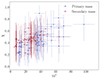Fig. 1. Mass-spin dataset: Scatter plot of the 59 GW events used in the analysis. They correspond to the BBH GW events from GWTC-3 catalog, selected with an IFAR ≥ 1 yr. The x axis shows the source frame masses ms and the y axis displays the spin magnitudes, χ. The errors bars are the 1σ uncertainties of the official LVK parameter estimation samples for each GW event.

3.1. Model selection

In Table 1, we report the log-Bayes factors and the maximum of log-likelihood ratios, between a baseline population model for which the spins are not correlated with the masses and the models we introduced in the previous section. The baseline model employed for this work is a single population described by one PLP distribution for the primary mass and the DEFAULT model for the spin parameters, following Abbott et al. (2023b).

The Bayes factors reveal that all the models that parameterize the spin-mass interplay as a transition between two subpopulations are strongly preferred against a model without any mass-spin correlation (despite the increased dimensionality of the fit). The EVOLVING GAUSSIAN model that parameterizes the spin-mass relation as a continuous evolution is neither preferred nor excluded by the data. To further validate the Bayes factor interpretation, we performed several tests reported in Appendix D. We verified that the preference of the Bayes factor is due to the inclusion of the spin-mass relation, as analyses with only mass information are not able to discriminate between the models. We have verified that our spin-mass models can also be confidently excluded when simulating a population of BBHs with no spin-mass correlation. Finally, we further verified that Bayes factors are inconclusive when blinding real data to possible spin-mass correlation, which was done by shuffling spin and mass estimations of real GW events.

3.2. Mass transition between two subpopulations

Figure 2 shows the reconstructed spin distributions for the EVOLVING GAUSSIAN, BETA TO GAUSSIAN, and BETA TO BETA models. All models find a transition from a population described by a low spin magnitude distribution to a population described by a higher and wider spin magnitude distribution. All three models infer that low spin magnitudes (around χ ∼ 0.2) are prevalent among compact objects with low masses, with a transition around 40−50 M_⊙. Beyond this threshold, the spin magnitude distribution shifts to include greater support for higher spin values. This evolution is particularly noticeable in the BETA TO BETA model, which excludes low spin magnitude values at high masses, while the other two models accommodate a wider range of spin magnitudes.

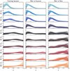Fig. 2. Evolving spin magnitude: Probability density functions of the spin magnitudes, χ, reconstructed from the population inference on 59 BBHs with an IFAR ≥ 1 yr from the GWTC-3 catalog, obtained with the EVOLVING GAUSSIAN (left column), BETA TO GAUSSIAN (middle column), and BETA TO BETA (right column) spin models. Each row represents a bin in source frame mass, from 10 M⊙ up to 100 M⊙, to highlight the spin-mass interplay.

The result of the EVOLVING GAUSSIAN model describes the spin-mass evolution in two possible ways (see Appendix C.1). Either the mean of the Gaussian does not evolve with the mass, but the width of the distribution increases, or the mean of the Gaussian evolves with the mass and the width is nearly fixed. Both scenarios produce an evolving spin magnitude distribution, but they cannot be disentangled yet from the current data.

The results from the (BETA TO BETA and BETA TO GAUSSIAN) models that parameterized a transition between two subpopulations (see Fig. 2), indicate a transition between two spin distributions between 40 and 55 M_⊙. From the current data, there is a preference for a steeper transition (∼10 M_⊙) around 40 M_⊙, rather than a slightly wider one (∼20 M_⊙) at 55 M_⊙ (see Appendix C.1). This indicates that the spin magnitude distribution of BHs at high masses is definitely higher than the one at low masses.

To understand if the spin-mass interplay is introduced by a wrong inference of the BBH mass spectrum, we compared the reconstructed mass distributions of our models with the ones of Abbott et al. (2023b). We find that the mass spectrum reconstructed by our models is in excellent agreement with the ones inferred in Abbott et al. (2023b) using an uncorrelated spin-mass model (see Appendix C.1).

3.3. Mixing of two independent subpopulations

The results from the previous section support a spin-mass interplay induced by a transition happening around 40−55 M_⊙ between two populations with different spin distributions. With the MIXTURE models, we studied if this relation could be consistent with the overlap of two independent BBH subpopulations, with separate and uncorrelated mass, spins, and redshift distributions, originating from distinct formation channels.

Figure 3 presents the reconstructed spin magnitudes and inclination angles inferred with each MIXTURE model flavor. For the MIXTURE VANILLA and MIXTURE PAIRED models, we set the primary population to describe the BBHs with masses ≲40 − 60 M_⊙. For the MIXTURE PEAK, the secondary population is described by a Gaussian peak in the 20 − 50 M_⊙ mass region (https://zenodo.org/records/14050137).

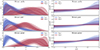Fig. 3. Mixture spin distributions: Probability density functions of the reconstructed spin magnitudes, χ, and the cosine of the tilt angles for each of the three mixture inferences, obtained on the 59 BBHs with an IFAR ≥ 1 yr from the GWTC-3 catalog. The red curves (Pop1) are the spin magnitudes and tilt angles found for the first population and the blue curves (Pop2) for the second population. The light blue curves (Total) are the combined distributions. The contours are the 90% and 95% confidence intervals.

The common result among the MIXTURE models is that the primary population of BBHs, which describes the large fraction of objects at small masses, supports low spin magnitudes peaking around χ ∼ 0.2, while the secondary population at higher masses supports a spin distribution of χ around 0.7. In all scenarios, the data indicates that the first population accounts for almost 98% of the overall population. The posteriors of the mixing fractions and their interplay with other population parameters are shown in Appendix C.2.

With the MIXTURE models, we also reconstructed the spin’s tilt angle distributions. Interestingly, the inferred distributions for the primary (low-mass) population weakly prefer spins aligned with the orbital angular momentum, while the secondary (high-mass) population weakly prefers a more isotropic distribution. We note, however, that the reconstructions of the spins’ tilt angle are still too uncertain to draw any robust conclusion (Vitale et al. 2022). Finally, we verified that the reconstructed mass and redshift distributions are consistent with the estimations obtained with non-evolving spin models and a single mass population (Abbott et al. 2023b) (see Appendix C.2).

4. Discussion

The spin-mass interplay can either be described as a mass-dependent transition between two spin populations, or as the overlap of two independent subpopulations with uncorrelated spin, mass, and redshift distributions. All the models infer a slowly spinning population of BBHs at low masses and another population of BBHs at higher masses with a spin population that can only be loosely constrained. We find a steep transition between the two BBH populations occurring around 40 − 55 M_⊙.

Previous studies have already tried to inspect a possible mass-spin relation at the population level of BBHs (Callister et al. 2021; Biscoveanu et al. 2022; Fishbach et al. 2022; Godfrey et al. 2023; Li et al. 2023). In Abbott et al. (2023b) and Tiwari (2022), it is argued that the absolute value of the “spin projection” over the orbital angular momentum does not significantly evolve with the chirp mass. This result is not in contrast with our findings (see Appendix C.1), as the spin tilt angles are poorly constrained. Therefore, the spin projection over the orbital angular momentum shows no particular correlation with the mass. The MIXTURE PEAK model is also consistent with the findings of Ray et al. (2024) that, using a binned nonparametric model, argues for the presence of a subpopulation of BBHs with a different spin distribution in the mass range of 30 − 40 M_⊙. Unlike our work, Ray et al. (2024) focuses on the effective and precession spin parameters, which are a combination of spin magnitudes, tilt angles, and masses. The results presented in Kimball et al. (2021) argue that the BBHs in GWTC-2 support a population composed of first-first generation, first-second generation, and second-second generation BHs. In Kimball et al. (2021), the mass and spin distributions of BBHs for first-first generation binaries were fit using phenomenological models, like the ones employed in this paper, while the first-second and second-second mass and spin distributions were obtained with transfer functions defined in Kimball et al. (2020) from the first-first generation binaries. In our study, we go beyond the use of a transfer function calibrated on hierarchical formation channels only and, using general phenomenological models, we demonstrate that there is a spin-mass relation that is probably introduced by the transition in mass between subpopulations described by different spin distributions.

In Li (2022) and Li et al. (2023), the investigation focuses on subpopulations of BBHs via a semi-parametric approach. They observe hints of a transition in mass between two spin distributions, while keeping the CBC merger rate constant and employing a single model for the tilt angle across both populations. Furthermore, our approach extends beyond theirs by exploring a wider range of scenarios and allowing for greater flexibility, and thus provides a more comprehensive and robust analysis of BBH subpopulations. We now speculate about the possible astrophysical implications of our results regarding the BBH formation channels. One of the most accepted theories for compact objects’ formation is that BHs from isolated stellar binaries cannot be formed beyond [45 − 60] M_⊙. This mass scale is identified as the lower edge of the PISN (Farmer et al. 2019, 2020; Renzo et al. 2020; Karathanasis et al. 2023). In this picture, the PISN mass scale would mark a transition between a population of first-generation BHs formed by their stellar progenitors to a population of n^th-generation BHs dynamically assembled into binaries (Mapelli 2021; Kimball et al. 2021) in dense stellar environments. The population of first-generation BBHs is predicted to have relatively small spins aligned with the orbital angular momentum (Mapelli 2021), due to the transfer of stellar material during the binary evolution. The population of n^th-generation BHs’ is expected to display spin magnitudes that are around 0.7 (from the pre-merger binary) and nearly isotropically distributed (Berti & Volonteri 2008; Gerosa & Berti 2017; Fishbach et al. 2017; Galvez Ghersi & Stein 2021). According to the latest BBH synthesis simulations, first-generation BBHs are expected to form 97.5–98% of the population, and n^th-generation the rest, all formation channels combined (Li 2022; Mapelli et al. 2021).

5. Conclusions

We observe a transition between two BBH subpopulations around 40 − 55 M_⊙. The lower-mass population exhibits a clear preference for low spin magnitudes (χ ∼ 0.1), as was expected from stellar-mass BHs. While the spin distribution for the higher-mass population is not as strongly constrained, but still certainly different from that of the low-mass population. Our findings, supported by MIXTURE models, indicate that the spin distribution for this higher-mass group tends toward values of around 0.7. We speculate that these results align with the hypothesis of a BBH population composed of BHs formed from isolated stellar binaries, as well as through dynamical assembly and hierarchical mergers. In this context, the MIXTURE models suggest that the high-mass (n^th-generation) population constitutes only 2% of the total astrophysical BBHs. Another significant finding obtained with the MIXTURE models is that the BBH merger rate, as a function of redshift, increases similarly for both low- and high-mass subpopulations. If we interpret the former as first-generation BHs and the latter as n^th-generation BHs, this result could suggest that the timescales for hierarchical mergers are cosmologically short. We speculate that our findings regarding the interplay between spin and mass support the existence of dynamically formed BBHs with masses exceeding 40 − 50 M_⊙. However, definitive evidence for this hypothesis would require a more accurate reconstruction of the spin-tilt distribution, which could be achieved through future GW observations.

Data availability

The additional supplementary material that support the findings of this study, and in particular the sanity checks and the prior ranges used to infer the population parameters, are openly available at https://zenodo.org/records/14050137

Acknowledgments

The authors are grateful for computational resources provided by the LIGO Laboratory and supported by the National Science Foundation Grants PHY-0757058 and PHY-0823459.

References

Appendix A: Inference framework

A.1. Hierarchical Bayesian inference

The detection of gravitational wave sources by current ground-based detectors can be described as an inhomogeneous Poisson process in the presence of selection biases. The central quantity of inference is the BBH merger rate

$$\begin{array}{c}\hfill \frac{\mathrm{d}{N}_{\mathrm{CBC}}}{\mathrm{d}\theta \mathrm{d}z\mathrm{d}{t}_s}(\mathrm{\Lambda }),\end{array}$$(A.1)

that we describe in terms of binary parameters θ (in this work, these are the source masses, spin magnitudes, tilt angles and CBC rate), redshift and source frame time. The BBH rate in Eq. A.1 is a function of the population parameters Λ, the rate models we employ in this work are described in Appendix B. We write the hyperlikelihood following Vitale et al. (2020) and Mandel & Farmer (2022)

$$\begin{array}{cc}\hfill \mathcal{L}(\{x\}|\mathrm{\Lambda })\propto & e^{-N_{\exp }(\mathrm{\Lambda })}{\displaystyle \prod _i^{N_{\mathrm{GW}}}{T}_{\mathrm{obs}}\int \mathrm{d}\theta \mathrm{d}z{\mathcal{L}}_{\mathrm{GW}}(x_i|\theta ,z)}\hfill \\ \hfill & \times \frac{1}{1+z}\frac{\mathrm{d}{N}_{\mathrm{CBC}}}{\mathrm{d}\theta \mathrm{d}z\mathrm{d}{t}_s}(\mathrm{\Lambda }).\hfill \end{array}$$(A.2)

In the above Eq. A.2, ℒ_GW(x_i|θ, z) is the GW likelihood, which quantifies the errors on the estimation of the θ and z parameters from the data. The term N_exp takes into account the selection effects, introduced due to the finite sensitivity of the detectors,

$$\begin{array}{c}\hfill N_{\exp }(\mathrm{\Lambda })=T_{\mathrm{obs}}{\displaystyle \int }\mathrm{d}\theta \mathrm{d}z{P}_{\det }(\theta ,z)\frac{1}{1+z}\frac{\mathrm{d}{N}_{\mathrm{CBC}}}{\mathrm{d}z\mathrm{d}\theta \mathrm{d}{t}_s}(\mathrm{\Lambda }),\end{array}$$(A.3)

where the detection probability P_det(z, θ) represents the probability that an event characterized by its true binary parameters θ at redshift z is detected; that is, it overpasses some chosen detection threshold adopted by the search algorithm (e.g., the signal to noise ratio, SNR, or the inverse false alarm rate, IFAR).

The hierarchical likelihood is evaluated numerically for each population model using a set of parameter estimation samples from N_GW GW events and a set of detectable injections that are used to evaluate selection biases. Each injection and parameter estimation sample consists in a value for the parameters θ and z, that is used to evaluate the BBH merger rate in Eq. A.1 (Mastrogiovanni et al. 2024) and to deconvolve the priors π_PE and π_inj that are used to generate the parameter estimation samples and the injections. The overall likelihood is numerically approximated via Monte-Carlo sampling as

$$\begin{array}{c}\hfill ln[\mathcal{L}(\{x\}|\mathrm{\Lambda })]\approx -\frac{T_{\mathrm{obs}}}{N_{\mathrm{gen}}}{\displaystyle \sum _{j=1}^{N_{\det }}{s}_j+\sum _i^{N_{\mathrm{obs}}}ln\left[\frac{T_{\mathrm{obs}}}{N_{\mathrm{s},i}}\sum _{j=1}^{N_{\mathrm{s},i}}{w}_{i,j}\right],}\end{array}$$(A.4)

where s_j and w_i, j are the weights associated to the injections and parameter estimation samples, the i index refers to the i-th event, while j to the Monte-Carlo sampling:

$$\begin{array}{cc}\hfill s_j& =\frac{1}{{\pi }_{\mathrm{inj}}({\theta }_j,z_j)}\frac{1}{1+z_j}\frac{\mathit{dN}}{d{t}_{s}dzd\theta }(\mathrm{\Lambda }){|}_j\hfill \end{array}$$(A.5)

$$\begin{array}{cc}\hfill w_{i,j}& =\frac{1}{{\pi }_{\mathrm{PE}}({\theta }_{i,j},z_{i,j}|\mathrm{\Lambda })}\frac{1}{1+z_{i,j}}\frac{\mathit{dN}}{\mathrm{d}{t}_s\mathrm{d}\theta \mathrm{d}z}(\mathrm{\Lambda }){|}_{i,j}\hfill \end{array}$$(A.6)

In our analyses, we apply a set of criteria to check the numerical stability of Eq. A.4. In particular, we require that at least ten parameter estimation samples per GW event contribute to the numerical evaluation of the likelihood and at least 200 injections for the calculation of the selection biases (Farr 2019).

A.2. Numerical stability tests

To test the numerical stability of our results, we conducted two supplementary analyses, without applying any cuts to our stability estimators: the effective number of samples for the GW events (${\mathrm{N}}_{\mathrm{eff}}^{\mathrm{PE}}$) and the effective number of injections (${\mathrm{N}}_{\mathrm{eff}}^{\mathrm{inj}}$). In the main analysis, these parameters were set to ${\mathrm{N}}_{\mathrm{eff}}^{\mathrm{PE}}=10$ and ${\mathrm{N}}_{\mathrm{eff}}^{\mathrm{inj}}=4{\mathrm{N}}_{\mathrm{GW}}$. Figures A.1 and A.2 show the estimated distributions of key population parameters alongside the two stability estimators. We compared the estimated posteriors using the same 59 GW events with the BETA TO BETA and MIXTURE VANILLA models, respectively. We do not observe any significant correlation between the population parameters and the stability estimators, indicating that the spin evolution part of the parameter space is not influenced by ${\mathrm{N}}_{\mathrm{eff}}^{\mathrm{inj}}$ or ${\mathrm{N}}_{\mathrm{eff}}^{\mathrm{PE}}$. Furthermore, removing these cuts did not cause the hierarchical likelihood to shift to a different part of the parameter space, as the posterior distributions remained very similar with and without the stability cuts. We conclude that the results obtained are stable with respect to the numerical stability of the hierarchical Bayesian inference.

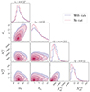Fig. A.1. Corner plot EVOLVING MODEL: Corner plot of the population parameters (mt,δmt) and the stability estimator ($N_{\mathrm{eff}}^{\mathrm{inj}}$,$N_{\mathrm{eff}}^{\mathrm{PE}}$), obtained with the BETA TO BETA evolving model on the 59 GW events with IFAR ≥ 1 yr. The purple contours and histograms were estimated while putting the minimum value of $N_{\mathrm{eff}}^{\mathrm{inj}}=200$ and $N_{\mathrm{eff}}^{\mathrm{PE}}=10$. The pink contours and histograms were estimated while placing not cuts on these estimators.

Fig. A.2. Corner plot MIXTURE MODEL: Corner plot of the population parameters (mt,δmt) and the stability estimator ($N_{\mathrm{eff}}^{\mathrm{inj}}$,$N_{\mathrm{eff}}^{\mathrm{PE}}$), obtained with the MIXTURE VANILLA evolving model on the 59 GW events with IFAR ≥ 1 yr. The purple contours and histograms were estimated while putting the minimum value of $N_{\mathrm{eff}}^{\mathrm{inj}}=200$ and $N_{\mathrm{eff}}^{\mathrm{PE}}=10$. The pink contours and histograms were estimated while placing not cuts on these estimators.

Appendix B: Population models and priors

In our analysis, we use three families of population models to parameterize the BBH merger rate given in Eq. A.1. The first class has only one population, the VANILLA model, that describes the spin, redshift and mass distributions independent of each other and uncorrelated. The second class, EVOLVING models, includes three population models that describe the mass and spin distribution as independent while modeling the spin distribution with an analytical dependence from the mass. The third class, MIXTURE models, describe the overall BBH merger rate as the superposition of two independent subpopulations with uncorrelated mass, spins and redshift distributions.

B.1. Vanilla model

The BBH rate function is described as

$$\begin{array}{c}\hfill \frac{\mathrm{d}{N}_{\mathrm{CBC}}}{\mathrm{d}\theta \mathrm{d}z\mathrm{d}{t}_s}(\mathrm{\Lambda })=R(z;\mathrm{\Lambda })\frac{\mathrm{d}{V}_c}{\mathrm{d}z}{p}_{\mathrm{pop}}({\overrightarrow{m}}_s|\mathrm{\Lambda })\pi (\overrightarrow{\chi },cos\overrightarrow{\theta }|\mathrm{\Lambda }),\end{array}$$(B.1)

where the vectors indicate the components of the two binary masses, spin magnitudes and tilt angles. The priors used for this run are listed in Appendix E.

The rate function is modeled after an MD (MD; Madau & Dickinson 2014) star formation rate s.t.

$$\begin{array}{c}\hfill R(z;\mathrm{\Lambda })=R_0[1+{(1+z_p)}^{-\gamma -k}]\frac{{(1+z)}^{\gamma }}{1+{\left(\frac{1+z}{1+z_p}\right)}^{\gamma +k}}.\end{array}$$(B.2)

The mass distribution is modeled according to a POWER LAW + PEAK model with

$$\begin{array}{cc}\hfill \pi (m_{1,s}|m_{\min },m_{\max },\alpha )& =(1-\lambda )\mathcal{P}(m_{1,s}|m_{\min },m_{\max },-\alpha )+\hfill \\ \hfill & \lambda \mathcal{G}(m_{1,s}|{\mu }_g,\sigma ),(0\le \lambda \le 1)\hfill \end{array}$$(B.3)

$$\begin{array}{cc}\hfill \pi (m_{2,s}|m_{\min },m_{1,s},\beta )& =\mathcal{P}(m_{2,s}|m_{\min },m_{1,s},\beta ).\hfill \end{array}$$(B.4)

where 𝒫 is a truncated powerlaw and 𝒢 a Gaussian. The mass distribution also includes a tapering at low masses governed by a population parameter δ_m, which is defined such that:

$$\begin{array}{cc}\hfill \pi (m_{1,s},m_{2,s}|\mathrm{\Lambda })& =\pi (m_{1,s}|\mathrm{\Lambda })\pi (m_{2,s}|m_{1,s},\mathrm{\Lambda })\times \hfill \\ \hfill & S(m_1|m_{\min },{\delta }_m)S(m_2|m_{\min },{\delta }_m),\hfill \end{array}$$(B.5)

where S is a sigmoid window function. The parameterization of the window function is taken from Abbott et al. (2021) and has the following form

$$\begin{array}{cc}& S(m|m_{\min },{\delta }_m)=\hfill \\ \hfill & =\{\begin{array}{cc}0,\hfill & \hfill (m<m_{\min })\\ {[f(m-m_{\min },{\delta }_m)+1]}^{-1},\hfill & \hfill (m_{\min }\le m<m_{\min }+{\delta }_m)\\ 1,\hfill & \hfill (m\ge m_{\min }+{\delta }_m)\end{array}\hfill \end{array}$$(B.6)

with

$$\begin{array}{c}\hfill f(m\prime ,{\delta }_m)=exp(\frac{{\delta }_m}{m\prime }+\frac{{\delta }_m}{m\prime -{\delta }_m}).\end{array}$$(B.7)

The spin distribution is modeled according to the DEFAULT spin model of Talbot et al. (2019) and Wysocki et al. (2019) as

$$\begin{array}{cc}\hfill \pi (\overrightarrow{\chi },cos\overrightarrow{\theta }|\mathrm{\Lambda })=& \mathrm{Beta}({\chi }_1|\alpha ,\beta )\mathrm{Beta}({\chi }_2|\alpha ,\beta )\times \hfill \\ \hfill & \pi (cos\overrightarrow{\theta }|\xi ,{\sigma }_t),\hfill \end{array}$$(B.8)

with

$$\begin{array}{c}\hfill \pi (cos{\theta }_{1,2}|\zeta ,{\sigma }_t)=\xi {\mathcal{G}}_{[-1,1]}(cos{\theta }_{1,2}|1,{\sigma }_t)+\frac{1-\xi }{2},\end{array}$$(B.9)

where 𝒢_{[ − 1, 1]}(cos θ_i|1, σ_t) is a truncated Gaussian between −1 and 1.

B.2. Evolving models

The BBH rate function is described as

$$\begin{array}{c}\hfill \frac{\mathrm{d}{N}_{\mathrm{CBC}}}{\mathrm{d}\theta \mathrm{d}z\mathrm{d}{t}_s}(\mathrm{\Lambda })=R(z;\mathrm{\Lambda })\frac{\mathrm{d}{V}_c}{\mathrm{d}z}{p}_{\mathrm{pop}}({\overrightarrow{m}}_s|\mathrm{\Lambda })\pi (\overrightarrow{\chi },cos\overrightarrow{\theta }|\overrightarrow{m},\mathrm{\Lambda }),\end{array}$$(B.10)

Differently from the vanilla case, the spin for this class of models is conditioned on the value of the source mass. For all the models, the spin distribution is factorized as

$$\begin{array}{c}\hfill \pi (\overrightarrow{\chi },cos\overrightarrow{\theta }|\overrightarrow{m},\mathrm{\Lambda })=\pi (\overrightarrow{\chi }|\overrightarrow{m},\mathrm{\Lambda })\pi (cos\overrightarrow{\theta }|,\mathrm{\Lambda }),\end{array}$$(B.11)

where the spin magnitude probability is conditioned on the mass values (see below for the models) and the angular distribution $\pi (cos\overrightarrow{\theta }|,\mathrm{\Lambda })$ is not dependent on the mass, and it is the one for the DEFAULT model. Moreover, all the models assume that

$$\begin{array}{c}\hfill \pi (\overrightarrow{\chi }|\overrightarrow{m},\mathrm{\Lambda })=\pi ({\chi }_1|m_1,\mathrm{\Lambda })\pi ({\chi }_2|m_2,\mathrm{\Lambda }).\end{array}$$(B.12)

For all the EVOLVING models, we use the rate model in Eq. B.2 and the mass spectrum described by the POWER LAW + PEAK in Eqs. B.3 and B.4. The priors used for this run are listed in Appendix E. Below we describe what parameterization is used for the spin magnitude distribution.

B.2.1. Evolving Gaussian

The EVOLVING Gaussian model parameterizes the spin magnitudes distribution as a truncated Gaussian between 0 and 1 with a mass varying mean and standard deviation, namely

$$\begin{array}{c}\hfill \pi (\chi |m,\mathrm{\Lambda })={\mathcal{G}}_{[0,1]}(\chi |\mu (m),\sigma (m)).\end{array}$$(B.13)

The mass-varying mean and standard deviation are approximated at the linear with a first order Taylor’s expansion.

$$\begin{array}{cc}\hfill \mu (m)& ={\mu }_0+\dot{\mu }m\hfill \end{array}$$(B.14)

$$\begin{array}{cc}\hfill \sigma (m)& ={\sigma }_0+\dot{\sigma }m.\hfill \end{array}$$(B.15)

For this model, ${\mu }_0,{\sigma }_0,\dot{\mu },\dot{\sigma }$ are additional population parameters.

B.2.2. Beta to Gaussian

This model parameterizes the spin magnitude distribution as a mass-dependent transition from a spin population described by a Beta(χ|α, β) distribution to a spin population described by a truncated Gaussian 𝒢_[0, 1](χ|μ, σ). The spin distribution is given by

$$\begin{array}{cc}\hfill \pi (\chi |m,\mathrm{\Lambda })=& W(z;m_{\mathrm{t}},\delta m_{\mathrm{t}})B(\chi |\alpha ,\beta )\hfill \\ \hfill & +(1-W(z;m_{\mathrm{t}},\delta m_{\mathrm{t}})){\mathcal{G}}_{[0,1]}(\chi |\mu ,\sigma ),\hfill \end{array}$$(B.16)

where W(z; m_t, δm_t) is a logistic function that smoothly transitions from 1 to 0. The window function is defined as

$$\begin{array}{c}\hfill W(z;m_{\mathrm{t}},\delta m_{\mathrm{t}})=\frac{1}{1+e^{\frac{m-m_{\mathrm{t}}}{\delta m_{\mathrm{t}}}}}.\end{array}$$(B.17)

B.2.3. Beta to Beta

This model is similar to the BETA TO GAUSSIAN but instead, it parameterizes the spin function as transitioning between two Beta distributions, namely

$$\begin{array}{cc}\hfill \pi (\chi |m,\mathrm{\Lambda })=& W(z;m_{\mathrm{t}},\delta m_{\mathrm{t}})B(\chi |{\alpha }_1,{\beta }_1)\hfill \\ \hfill & +(1-W(z;m_{\mathrm{t}},\delta m_{\mathrm{t}}))B(\chi |{\alpha }_2,{\beta }_2).\hfill \end{array}$$(B.18)

The window function is defined as in the previous case.

B.3. Mixture models

This class of models parameterizes the BBH merger rate as the overlap of two subpopulations, population 1 (Pop1) and population 2 (Pop2). The BBH merger rate is given by

$$\begin{array}{c}\hfill \frac{\mathrm{d}{N}_{\mathrm{CBC}}}{\mathrm{d}\theta \mathrm{d}z\mathrm{d}{t}_s}={\lambda }_{\mathrm{pop}}\frac{\mathrm{d}{N}_{\mathrm{CBC}}}{\mathrm{d}\theta \mathrm{d}z\mathrm{d}{t}_s}({\mathrm{\Lambda }}^{\mathrm{Pop}1})+(1-{\lambda }_{\mathrm{pop}})\frac{\mathrm{d}{N}_{\mathrm{CBC}}}{\mathrm{d}\theta \mathrm{d}z\mathrm{d}{t}_s}({\mathrm{\Lambda }}^{\mathrm{Pop}2}),\end{array}$$(B.19)

where the parameter λ_pop parameterizes the mixture fraction between the two subpopulations. The parameters Λ^Pop1, Λ^Pop2 collectively indicate the population parameters of the two subpopulations that are independent of each other. The MIXTURE models parameterize the subpopulation merger rates with distributions of mass, spin and redshift that are uncorrelated. The specific factorization of the subpopulation merger rates is described in the section below and the priors and population parameters used are shown in Appendix E.

B.3.1. Mixture vanilla

The MIXTURE VANILLA model parameterizes the distribution of the first population using a POWER LAW + PEAK for the primary and secondary mass distributions as in Eqs. B.3 and B.4, a DEFAULT spin model for the spin magnitudes and orientation, a MD rate for the BBH merger rate. The second population is modeled with a mass spectrum described with a truncated power law for the primary mass, and the secondary mass has a distribution has an equivalent distribution to the one in Eq. B.4. The spin magnitudes and orientation follow a DEFAULT model and a MD rate function for the BBH merger rate.

B.3.2. Mixture peak

The MIXTURE PEAK model parameterizes the distribution of the first population using a power law for the primary mass and secondary mass distribution as in Eq. B.4. The spin magnitudes and orientation are distributed according to a DEFAULT model and the BBH rate function as a MD rate. The second population is modeled with a mass spectrum described by the primary and secondary masses distributed according to a Gaussian with mean μ_g and standard deviation μ_g. An additional constraint is set on the Gaussian mass distribution to ensure that m₁ > m₂. The spin magnitudes and orientation follow a DEFAULT spin model and a MD rate function for the BBH merger rate.

B.3.3. Mixture pairing

The MIXTURE PAIRING model is a variation of the MIXTURE VANILLA model. The distributions of spins, redshift and primary masses of the two subpopulations are still described as in the MIXTURE VANILLA model, with the difference that the secondary mass is forced to have the same distribution as the primary mass. In other words, the mass distribution is generally factorized as

$$\begin{array}{c}\hfill p_{\mathrm{pop}}(m_1,m_2|\mathrm{\Lambda })\propto p_{\mathrm{pop}}(m_1|\mathrm{\Lambda })p_{\mathrm{pop}}(m_2|\mathrm{\Lambda }){\left[\frac{m_2}{m_1}\right]}^{\beta }\mathrm{\Theta }(m_1-m_2),\end{array}$$(B.20)

where Θ is an Heaviside step function forcing m₁ > m₂ and an additional weight dependent on the two masses ratio is included.

All Tables

All Figures

	Fig. 1. Mass-spin dataset: Scatter plot of the 59 GW events used in the analysis. They correspond to the BBH GW events from GWTC-3 catalog, selected with an IFAR ≥ 1 yr. The x axis shows the source frame masses ms and the y axis displays the spin magnitudes, χ. The errors bars are the 1σ uncertainties of the official LVK parameter estimation samples for each GW event.
In the text

Fig. 2. Evolving spin magnitude: Probability density functions of the spin magnitudes, χ, reconstructed from the population inference on 59 BBHs with an IFAR ≥ 1 yr from the GWTC-3 catalog, obtained with the EVOLVING GAUSSIAN (left column), BETA TO GAUSSIAN (middle column), and BETA TO BETA (right column) spin models. Each row represents a bin in source frame mass, from 10 M⊙ up to 100 M⊙, to highlight the spin-mass interplay.

In the text

Fig. 3. Mixture spin distributions: Probability density functions of the reconstructed spin magnitudes, χ, and the cosine of the tilt angles for each of the three mixture inferences, obtained on the 59 BBHs with an IFAR ≥ 1 yr from the GWTC-3 catalog. The red curves (Pop1) are the spin magnitudes and tilt angles found for the first population and the blue curves (Pop2) for the second population. The light blue curves (Total) are the combined distributions. The contours are the 90% and 95% confidence intervals.

In the text

Fig. A.1. Corner plot EVOLVING MODEL: Corner plot of the population parameters (mt,δmt) and the stability estimator ($N_{\mathrm{eff}}^{\mathrm{inj}}$,$N_{\mathrm{eff}}^{\mathrm{PE}}$), obtained with the BETA TO BETA evolving model on the 59 GW events with IFAR ≥ 1 yr. The purple contours and histograms were estimated while putting the minimum value of $N_{\mathrm{eff}}^{\mathrm{inj}}=200$ and $N_{\mathrm{eff}}^{\mathrm{PE}}=10$. The pink contours and histograms were estimated while placing not cuts on these estimators.

In the text

Fig. A.2. Corner plot MIXTURE MODEL: Corner plot of the population parameters (mt,δmt) and the stability estimator ($N_{\mathrm{eff}}^{\mathrm{inj}}$,$N_{\mathrm{eff}}^{\mathrm{PE}}$), obtained with the MIXTURE VANILLA evolving model on the 59 GW events with IFAR ≥ 1 yr. The purple contours and histograms were estimated while putting the minimum value of $N_{\mathrm{eff}}^{\mathrm{inj}}=200$ and $N_{\mathrm{eff}}^{\mathrm{PE}}=10$. The pink contours and histograms were estimated while placing not cuts on these estimators.

In the text

References

- Abbott, B. P., Abbott, R., Abbott, T. D., et al. 2018, Liv. Rev. Relat., 21, 3 [NASA ADS] [CrossRef] [Google Scholar]
- Abbott, R., Abbott, T. D., Abraham, S., et al. 2021, ApJ, 913, L7 [NASA ADS] [CrossRef] [Google Scholar]
- Abbott, R., Abbott, T. D., Acernese, F., et al. 2023a, Phys. Rev. X, 13, 041039 [Google Scholar]
- Abbott, R., Abbott, T. D., Acernese, F., et al. 2023b, Phys. Rev. X, 13, 011048 [NASA ADS] [Google Scholar]
- Abbott, R., Abe, H., Acernese, F., et al. 2023c, ApJS, 267, 29 [CrossRef] [Google Scholar]
- Adamcewicz, C., & Thrane, E. 2022, MNRAS, 517, 3928 [NASA ADS] [CrossRef] [Google Scholar]
- Adamcewicz, C., Lasky, P. D., & Thrane, E. 2023, ApJ, 958, 13 [NASA ADS] [CrossRef] [Google Scholar]
- Adamcewicz, C., Galaudage, S., Lasky, P. D., & Thrane, E. 2024, ApJ, 964, L6 [NASA ADS] [CrossRef] [Google Scholar]
- Ashton, G., Hübner, M., Lasky, P. D., et al. 2019, ApJS, 241, 27 [NASA ADS] [CrossRef] [Google Scholar]
- Bartos, I., Kocsis, B., Haiman, Z., & Márka, S. 2017, ApJ, 835, 165 [Google Scholar]
- Berti, E., & Volonteri, M. 2008, ApJ, 684, 822 [NASA ADS] [CrossRef] [Google Scholar]
- Biscoveanu, S., Callister, T. A., Haster, C.-J., et al. 2022, ApJ, 932, L19 [NASA ADS] [CrossRef] [Google Scholar]
- Bouffanais, Y., Mapelli, M., Santoliquido, F., et al. 2021, MNRAS, 507, 5224 [NASA ADS] [CrossRef] [Google Scholar]
- Callister, T. A., Haster, C.-J., Ng, K. K. Y., Vitale, S., & Farr, W. M. 2021, ApJ, 922, L5 [NASA ADS] [CrossRef] [Google Scholar]
- Callister, T. A., Miller, S. J., Chatziioannou, K., & Farr, W. M. 2022, ApJ, 937, L13 [NASA ADS] [CrossRef] [Google Scholar]
- Cheng, A. Q., Zevin, M., & Vitale, S. 2023, ApJ, 955, 127 [NASA ADS] [CrossRef] [Google Scholar]
- Farah, A. M., Callister, T. A., Ezquiaga, J. M., Zevin, M., & Holz, D. E. 2024, ArXiv e-prints [arXiv:2404.02210] [Google Scholar]
- Farmer, R., Renzo, M., de Mink, S. E., Marchant, P., & Justham, S. 2019, ArXiv e-prints [arXiv:1910.12874] [Google Scholar]
- Farmer, R., Renzo, M., de Mink, S., Fishbach, M., & Justham, S. 2020, ApJ, 902, L36 [CrossRef] [Google Scholar]
- Farr, W. M. 2019, Res. Notes AAS, 3, 66 [NASA ADS] [CrossRef] [Google Scholar]
- Fishbach, M., & Holz, D. E. 2020, ApJ, 891, L27 [NASA ADS] [CrossRef] [Google Scholar]
- Fishbach, M., Holz, D. E., & Farr, B. 2017, ApJ, 840, L24 [NASA ADS] [CrossRef] [Google Scholar]
- Fishbach, M., Kimball, C., & Kalogera, V. 2022, ApJ, 935, L26 [NASA ADS] [CrossRef] [Google Scholar]
- Galvez Ghersi, J. T., & Stein, L. C. 2021, Class. Quant. Grav., 38, 045012 [NASA ADS] [CrossRef] [Google Scholar]
- Gerosa, D., & Berti, E. 2017, Phys. Rev. D, 95, 124046 [NASA ADS] [CrossRef] [Google Scholar]
- Gerosa, D., & Fishbach, M. 2021, Nat. Astron., 5, 749 [NASA ADS] [CrossRef] [Google Scholar]
- Godfrey, J., Edelman, B., & Farr, B. 2023, ArXiv e-prints [arXiv:2304.01288] [Google Scholar]
- Karathanasis, C., Mukherjee, S., & Mastrogiovanni, S. 2023, MNRAS, 523, 4539 [NASA ADS] [Google Scholar]
- Kimball, C., Talbot, C., Berry, C. P. L., et al. 2020, ApJ, 900, 177 [NASA ADS] [CrossRef] [Google Scholar]
- Kimball, C., Talbot, C., Berry, C. P. L., et al. 2021, ApJ, 915, L35 [CrossRef] [Google Scholar]
- Li, G.-P. 2022, A&A, 666, A194 [NASA ADS] [CrossRef] [EDP Sciences] [Google Scholar]
- Li, Y. J., Wang, Y. Z., Tang, S. P., & Fan, Y. Z. 2023, ArXiv e-prints [arXiv:2303.02973] [Google Scholar]
- Madau, P., & Dickinson, M. 2014, ARA&A, 52, 415 [Google Scholar]
- Mandel, I., & Farmer, A. 2022, Phys. Rep., 955, 1 [NASA ADS] [CrossRef] [Google Scholar]
- Mapelli, M. 2020, Front. Astron. Space Sci., 7, 38 [NASA ADS] [CrossRef] [Google Scholar]
- Mapelli, M. 2021, ArXiv e-prints [arXiv:2106.00699] [Google Scholar]
- Mapelli, M., Dall’Amico, M., Bouffanais, Y., et al. 2021, MNRAS, 505, 339 [CrossRef] [Google Scholar]
- Marchant, P., Langer, N., Podsiadlowski, P., Tauris, T. M., & Moriya, T. J. 2016, A&A, 588, A50 [NASA ADS] [CrossRef] [EDP Sciences] [Google Scholar]
- Mastrogiovanni, S., Laghi, D., Gray, R., et al. 2023, Phys. Rev. D, 108, 042002 [NASA ADS] [CrossRef] [Google Scholar]
- Mastrogiovanni, S., Pierra, G., Perriès, S., et al. 2024, A&A, 682, A167 [NASA ADS] [CrossRef] [EDP Sciences] [Google Scholar]
- Mould, M., Gerosa, D., Broekgaarden, F. S., & Steinle, N. 2022, MNRAS, 517, 2738 [CrossRef] [Google Scholar]
- Planck Collaboration XIII. 2016, A&A, 594, A13 [NASA ADS] [CrossRef] [EDP Sciences] [Google Scholar]
- Ray, A., Hernandez, I. M., Breivik, K., & Creighton, J. 2024, ArXiv e-prints [arXiv:2404.03166] [Google Scholar]
- Renzo, M., Farmer, R. J., Justham, S., et al. 2020, MNRAS, 493, 4333 [NASA ADS] [CrossRef] [Google Scholar]
- Rinaldi, S., & Del Pozzo, W. 2021, MNRAS, 509, 5454 [NASA ADS] [CrossRef] [Google Scholar]
- Talbot, C., Smith, R., Thrane, E., & Poole, G. B. 2019, Phys. Rev. D, 100, 043030 [NASA ADS] [CrossRef] [Google Scholar]
- Thrane, E., & Talbot, C. 2019, PASA, 36, e010 [Erratum: PASA 37, e036 (2020)] [NASA ADS] [CrossRef] [Google Scholar]
- Tiwari, V. 2022, ApJ, 928, 155 [NASA ADS] [CrossRef] [Google Scholar]
- Tong, H., Galaudage, S., & Thrane, E. 2022, Phys. Rev. D, 106, 103019 [NASA ADS] [CrossRef] [Google Scholar]
- Vitale, S., Gerosa, D., Farr, W. M., & Taylor, S. R. 2020, ArXiv e-prints [arXiv:2007.05579] [Google Scholar]
- Vitale, S., Biscoveanu, S., & Talbot, C. 2022, A&A, 668, L2 [NASA ADS] [CrossRef] [EDP Sciences] [Google Scholar]
- Wen, L. 2003, ApJ, 598, 419 [NASA ADS] [CrossRef] [Google Scholar]
- Wysocki, D., Lange, J., & O’Shaughnessy, R. 2019, Phys. Rev. D, 100, 043012 [NASA ADS] [CrossRef] [Google Scholar]
- Zevin, M., Pankow, C., Rodriguez, C. L., et al. 2017, ApJ, 846, 82 [NASA ADS] [CrossRef] [Google Scholar]
- Zevin, M., Bavera, S. S., Berry, C. P. L., et al. 2021, ApJ, 910, 152 [Google Scholar]