| Issue |
A&A
Volume 694, February 2025
|
|
|---|---|---|
| Article Number | A186 | |
| Number of page(s) | 12 | |
| Section | Stellar structure and evolution | |
| DOI | https://doi.org/10.1051/0004-6361/202451654 | |
| Published online | 11 February 2025 | |
Compactness peaks: An astrophysical interpretation of the mass distribution of merging binary black holes
1
Laboratoire Lagrange, Université Côte d’Azur, Observatoire de la Côte d’Azur, CNRS, Bd de l’Observatoire, 06300 Nice, France
2
Laboratoire Artemis, Université Côte d’Azur, Observatoire de la Côte d’Azur, CNRS, Bd de l’Observatoire, 06300 Nice, France
⋆ Corresponding authors; This email address is being protected from spambots. You need JavaScript enabled to view it.
Received:
25
July
2024
Accepted:
22
October
2024
Abstract
With the growing number of detections of binary black hole (BBH) mergers, we are beginning to probe structure in the distribution of mass. A recent study proposes that the isolated binary evolution of stripped stars naturally gives rise to the peaks at ℳ ∼ 8 M⊙ and 14 M⊙ in the chirp-mass distribution and explains the dearth of black holes (BHs) in the mass range of ℳ ≈ 10 − 12 M⊙. The gap in chirp mass results from an apparent gap in the component-mass distribution within m1, m2 ≈ 10 − 15 M⊙ and the specific pairing of these BHs. This component-mass gap results from variation in the core compactness of the progenitor, where a drop in compactness as a function of carbon–oxygen core mass means that BHs are no longer formed from core collapse. We develop a population model motivated by this scenario to probe the structure of the component-mass distribution of two populations of BBHs: one population consisting of two peak components, representing BHs formed in the compactness peaks, and another population with a power-law component to account for any polluting events, that is, binaries that may have formed from different channels (e.g. dynamical). We perform hierarchical Bayesian inference to analyse the events from the third gravitational-wave transient catalogue (GWTC-3) with our population model. We find that there is a preference for the lower-mass peak to drop off sharply at ∼11 M⊙ and the upper mass peak to turn on at ∼13 M⊙, in line with predictions in the literature. However, we find no clear evidence for a gap. We also find mild support for a scenario where the two populations have different spin distributions. In addition to these population results, we highlight observed events of interest that differ from the expected population distribution of compact objects formed from stripped stars.
Key words: gravitational waves / binaries: close / stars: black holes / stars: evolution
© The Authors 2025
 Open Access article, published by EDP Sciences, under the terms of the Creative Commons Attribution License (https://creativecommons.org/licenses/by/4.0), which permits unrestricted use, distribution, and reproduction in any medium, provided the original work is properly cited.
This article is published in open access under the Subscribe to Open model. This email address is being protected from spambots. You need JavaScript enabled to view it. to support open access publication.
1. Introduction
Gravitational-wave astronomy is a rapidly growing field with approximately 90 detections (Abbott et al. 2023a) reported by the LIGO-Virgo-KAGRA collaboration (LVK). This catalogue of events was produced with data from the Advanced LIGO (Aasi et al. 2015) and Advanced Virgo (Acernese et al. 2015) gravitational-wave observatories. The majority of these detections are of merging binary black holes (BBHs). With population studies of these sources, the structure of the mass distribution of BBHs is slowly being revealed. This structure has implications for stellar physics processes, such as the explosion mechanisms of supernovae and mass-transfer processes in binaries (see Mapelli 2020; Mandel & Farmer 2022; Mandel & Broekgaarden 2022; Spera et al. 2022, for reviews).
The majority of the focus so far in terms of the astrophysical interpretation of these merging binaries has been in relation to the component masses of the compact binaries, with statistically significant peaks at ≈10 M⊙ and ≈35 M⊙ in the primary mass distribution (e.g. Talbot & Thrane 2018; Sadiq et al. 2022; Edelman et al. 2022; Wong & Cranmer 2022; Farah et al. 2023; Abbott et al. 2023b). The former peak may be associated with the binary mass-transfer processes (e.g. van Son et al. 2022), while the latter could be related to stellar physics, such as that regarding pulsational pair-instability supernovae (PPISNe; Heger & Woosley 2002; Croon & Sakstein 2023; Rahman et al. 2022), but there are suggestions that the fraction of events in this latter peak is too high for them to be PPISNe (e.g. Stevenson et al. 2019), that the location of the peak due to PPISNe should be higher (e.g. Farmer et al. 2020; Farag et al. 2022; Hendriks et al. 2023; Golomb et al. 2024), and that the peak is populated by merging binaries in globular clusters (Antonini et al. 2023). We note that there is also a possible peak at ∼16 − 20 M⊙ and an under-density at ∼14 M⊙ (Tiwari & Fairhurst 2021; Tiwari 2022, 2023; Abbott et al. 2023b), although these features are not statistically significant (e.g. Farah et al. 2023). Recent studies have, however, started to look beyond the component-mass distributions to investigate and interpret the chirp-mass distribution in more detail (e.g. Abbott et al. 2023b; Tiwari & Fairhurst 2021; Tiwari 2022, 2023; Schneider et al. 2023).
The chirp mass (Finn & Chernoff 1993; Poisson & Will 1995; Blanchet et al. 1995) determines the leading-order orbital evolution of a binary system from gravitational-wave emission and is therefore more accurately measured than the component masses,
 (1)
(1)
It is a combination of the individual component masses m1 and m2 and is directly related to gravitational-wave frequency and frequency evolution. The chirp-mass distribution of BBH mergers shows statistically significant peaks at 8, 14, and 28 M⊙, with an apparent lack of BBH mergers with ℳ ≈ 10 − 12 M⊙ (e.g. Abbott et al. 2023b; Tiwari 2023), which is hereafter referred to as the ‘chirp-mass gap’.
Schneider et al. (2023) recently proposed that merging BBHs formed via isolated binary evolution, where the progenitors lose their hydrogen-rich envelopes through mass-transfer processes, naturally give rise to the peaks at ℳ ∼ 8 M⊙ and 14 M⊙ and a dearth of BHs within the range of ℳ ≈ 10 − 12 M⊙. These authors find that the bimodality in the BBH chirp-mass distribution is due to the pairing of ‘compactness peaks’ in the component-mass distribution, which is linked to stellar physics and supernova mechanisms.
The explodability of stars is dependent on the compactness of the stellar core, ξ = (M/M⊙)/(R(M)/1000 km), where M is the mass of the core, and R(M) is the radius at the mass coordinate M, where M = 2.5 M⊙ is used in Schneider et al. (2023). The compactness is generally considered to not steadily increase with core mass, but rather to have sharp peaks and dips due to variations in burning stages in the core (e.g. O’Connor & Ott 2011; Sukhbold & Woosley 2014; Patton & Sukhbold 2020; Chieffi & Limongi 2020; Schneider et al. 2021, 2023; Burrows et al. 2023, 2024); however, there are studies in which a monotonic increase in compactness is considered (Mapelli et al. 2020). Considering the binary stripped stars in the Schneider et al. (2023) models, for 10% solar metallicity, the compactness level peaks due to neutrino-dominated burning of carbon–oxygen (CO) at core masses (MCO) of 7.5 M⊙, producing BHs from core collapse supernova at ≈9 − 10 M⊙; these are the low-mass BHs, which we refer to as BHL, which is the same notation as that used in Schneider et al. (2023). Above this core mass point, the compactness in the core drops, and this is a region where neutron stars are formed from core collapse rather than BHs (see Figure 3 in Schneider et al. 2023). At around MCO ≈ 13 M⊙, burning becomes neutrino dominated in the oxygen–neon (ONe) stage as well, producing BHs of greater than 15 M⊙ from core collapse supernova; these are the high-mass BHs, which we refer to as BHH. This variation in compactness level results in no BH masses being formed within ≈10 − 15 M⊙. These boundaries can shift due to uncertainties in the stellar physics, including that related to the metallicity-dependant mass-loss rate (Vink & de Koter 2005; Belczynski et al. 2010; Spera et al. 2015); convective core boundary mixing during core hydrogen and core helium burning (e.g. Schneider et al. 2023; Temaj et al. 2024), and 12C(α, γ)16O nuclear reaction rates (e.g. Farmer et al. 2019, 2020; Costa et al. 2021)1. However, the magnitude of the shifts at the lower-mass end are not expected to exceed ≈1 M⊙.
The peaks in chirp mass are produced by a mixture of pairings between BHL and BHH. The peak below the chirp-mass gap is formed by BHL + BHL and the structures above the chirp-mass gap are formed by BHH + BHH. Any BHL + BHH binaries are expected to fill this chirp-mass gap, but the pairing of BHL + BHH is less likely due to the fact that isolated binary evolution is more likely to produce systems with closer-to-equal mass ratios (Schneider et al. 2021). Assuming this model hypothesis is correct, the BHL + BHH population may be completely suppressed according to current observations (Abbott et al. 2023a).
In the present work, we develop a parametric population model motivated by the results of Schneider et al. in order to obtain an astrophysical interpretation of the mass distribution of BBH mergers. In Sect. 2 we provide a description of our population model and analysis method. In Sect. 3 we present our findings based on this model and compare them to results derived from models commonly used by the LVK. Finally, in Sect. 4 we discuss the astrophysical implications of our results and avenues for future work.
2. Methodology
In this work, we explore whether the findings of Schneider et al. (2023) can be used to explain the population of observed BBH mergers. To this end, we first investigate the properties of the events individually in Sect. 2.1. We then develop an astrophysically informed population model in Sect. 2.2 to investigate the properties of the population and to investigate whether or not there is a gap-like feature in the component-mass distribution.
2.1. Identifying binary black hole systems of interest
We consider the BBH mergers analysed in previous population studies (e.g. Abbott et al. 2023b), which include 69 BBH mergers from the third LVK gravitational-wave transient catalogue (GWTC-3; Abbott et al. 2023a) detected with a FAR < 1yr−1.
As an initial step, we find the positions of these events in the chirp-mass distribution and sort them according to whether they reside in the low- or high-mass region, as illustrated in the upper panel of Figure 1. We assume that those events in the low-mass region (ℳ < 11 M⊙) are BHL + BHL mergers and that those in the high-mass region (ℳ > 11 M⊙) are BHH + BHH mergers. We then show where these objects lie in the component-mass space. We find that from this first inspection, while there is a clear gap in the chirp-mass distribution, the component-mass distribution does not show a gap-like feature.
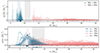 |
Fig. 1. Events in GWTC-3 with FAR < 1yr−1 sorted according to the chirp-mass peak in which they lie, assuming the Schneider et al. (2023) predictions regarding their classification and the locations of the gaps. Top panel: Chirp-mass posteriors showing the BHL + BHL (blue) and the BHH + BHH (pink). The grey shaded region represents the chirp-mass gap region (ℳ ≈ 10 − 12 M⊙). Bottom panel: Component-mass posteriors showing the BHL (blue) and the BHH (pink) BHs. The grey shaded region represents the expected component-mass gap region (m ≈ 10 − 15 M⊙). The vertical ticks illustrate the median of each posterior. |
We cannot robustly determine whether or not there exists a gap-like structure from visual inspection of the posteriors alone, especially given that the uncertainties on the mass posteriors are wider than the width of the gap. A population study, as outlined in Sect. 2.2, is required to investigate this structure. However, it is interesting to consider whether there are binaries ‘polluting’ the ≈10 − 15 M⊙ region in component mass that were formed via other channels.
We identify the events where the median of the mass posterior distribution (for one or both components) lies above 10 M⊙ for events with ℳ < 11 M⊙ and below 15 M⊙ for events with ℳ > 11 M⊙. We find 20 events that pollute the component-mass gap and list some of the properties in Table 1, including the mass ratio (q = m2/m1) and the effective inspiral spin (Santamaria et al. 2010; Ajith et al. 2011),
 (2)
(2)
Properties of events ‘polluting’ the component-mass gap (m = 10 − 15 M⊙).
a mass-weighted spin parameter that is projected along the orbital angular momentum, where χ is the spin magnitude and θ is the spin orientation, and the effective precession spin (Hannam et al. 2014; Schmidt et al. 2015)
![Mathematical equation: $$ \begin{aligned} \chi _{p} =\max \left[{\chi _1\sin \theta _1, q \frac{(3q + 4) }{(4q + 3)}}\chi _2\sin \theta _2 \right] ,\end{aligned} $$](/articles/aa/full_html/2025/02/aa51654-24/aa51654-24-eq63.gif) (3)
(3)
which is a measure of in-plane spin, and enables the parameterisation of the rate of relativistic precession of the orbital plane. These parameters may suggest the binary formed via a different channel. Mergers with an unequal mass ratio are unlikely to occur in isolated binary evolution (e.g. Kruckow et al. 2018; Giacobbo & Mapelli 2018; Broekgaarden et al. 2022; Iorio et al. 2023; Schneider et al. 2021). Negative values of χeff and large values of χp are generally considered to be a signature of dynamical formation given the support for misaligned and in-plane spin orientations (Mandel & O’Shaughnessy 2010; Rodriguez et al. 2016; Zevin et al. 2017; Rodriguez et al. 2018; Doctor et al. 2020).
We also indicate whether or not the events have been considered in other studies to have formed via a channel that is different from isolated binary evolution. To obtain a visual sense of these potential ‘pollutants’ (i.e. events that may not have formed via isolated binary evolution), we also provide the q, χeff, and χp distributions for these events in Figure 2 along with the median of the posterior for the other 49 events, which are illustrated by the black dots.
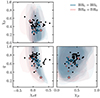 |
Fig. 2. Two-dimensional distributions of the mass ratio (q), effective inspiral spin (χeff), and effective precession spin (χp) of events polluting the m = 10 − 15 M⊙ gap (pink and blue shaded region; 90% credibility) and the median (pink and blue dots). The medians of the posteriors of the events outside the gap are also shown (black dots). Events polluting the gap (GW190412, GW151226, and GW200225), which may have formed via a channel different from isolated binary evolution, are highlighted with stars. |
There are a few events in the component-mass gap (Table 1) that appear to differ from the typical properties of systems formed via isolated evolution with more extreme mass ratios and/or higher values of χp (e.g. GW190412, GW151226, GW200225) compared to the rest of the BBH mergers populating the gap (see the blue and pinks dots in Figure 2). However, there are also events not in this mass gap that have these differing properties (black dots in Figure 2). Given this information, we need to build a population model that can account for potential pollutants in the population in addition to finding the location and edges of the compactness peaks. Finding this structure will help determine whether or not there is a gap-like feature within ≈10 − 15 M⊙ in the component-mass distribution of BBH mergers.
2.2. Building an astrophysically motivated population model
We developed an astrophysically informed population model incorporating the features predicted in Schneider et al. (2023) for the component-mass distributions while accounting for ‘pollutant’ events. We performed hierarchical Bayesian inference in order to measure the population hyper-parameters using gravitational-wave data from the LVK2. To this end, we used GWPopulation (Talbot et al. 2019), a hierarchical Bayesian inference package that employs Bilby (Ashton et al. 2019; Romero-Shaw et al. 2020). We use the nested sampler DYNESTY (Speagle 2020) for our analyses. Our dataset contains the 69 BBH observations from GWTC-3 (Abbott et al. 2023a) that were considered reliable for population analyses (events with a false-alarm rate of < 1 yr−1; Abbott et al. 2023b). We used the posterior samples from parameter estimation results used in Abbott et al. (2023b) along with the injection sets to account for selection effects (Essick & Farr 2022). There are three components to our model with various hyperparameters (Λ):
-
A low-mass narrow Gaussian (BHL Peak): this models the compactness peak where BHs are formed from increased compactness of CO cores of stars from neutrino-dominated burning,
 (4)
(4)where μBHL and σBHL are the mean and width of the Gaussian and mminBHL and mmaxBHL are its lower and upper limits.
-
A high-mass broad Gaussian (BHH Peak): this models the BHs formed from the increased compactness from neutrino release in the ONe burning stage,
 (5)
(5)where μBHH and σBHH are the mean and width of the Gaussian and mminBHH and mmaxBHH are its lower and upper limits.
-
A power-law component (Power Law or PL): this models everything that does not fit within these peaks, possibly from BHs formed via other channels,
 (6)
(6)where α is the slope index of the power law and mminBL and mmaxPL are its lower and upper truncation points.
Each of these components is paired with different mass-ratio distributions, where
 (7)
(7)
where X = BHL is the mass-ratio distribution for the low-mass Gaussian component, X = BHH is for the high-mass Gaussian component, and X = PL is for the power-law component. For each component, the mass ratio is constrained such that m2 also has to be larger than the minimum mass of that component mmin.
We consider the fraction of BBHs in each component, where fpeaks is the fraction of BBHs in the BHL and BHH peaks, and f1 is the fraction of BBHs in the BHL peak compared to the total number of BBHs in the two peaks. Therefore, the fraction of BBHs in the BHL peak, in the BHH peak, and in the power-law component are fBHL = fpeaks × f1, fBHH = fpeaks × (1 − f1), and fPL = 1 − fpeaks, respectively. Details on the prior ranges of these parameters are provided in Table A.1.
Considering our model, we may naively expect that the peaked distributions may have different spin properties compared to the power-law component. The peaked distributions are from BHs that form via isolated evolution, and therefore this population would generally be expected to form BBH systems with spins preferentially aligned with the orbital angular momentum. Supernova kicks may lead to misalignment of the spins, but the angle of this misalignment is generally considered to be modest (O’Shaughnessy et al. 2017; Stevenson et al. 2017; Gerosa et al. 2018; Rodriguez et al. 2016; Bavera et al. 2020). The BHs in the power-law component may have formed through different channels, and some may have formed dynamically. These systems are expected to form BH binaries with isotropically distributed spin orientations (Mandel & O’Shaughnessy 2010; Rodriguez et al. 2016; Zevin et al. 2017; Rodriguez et al. 2018; Doctor et al. 2020). If our sample contains hierarchical mergers, we may also expect to see greater spin magnitudes in this population (e.g. Yang et al. 2019; Gerosa & Berti 2017).
We consider two spin populations, one for the BBHs in the peaks (X = peaks), and one for the BBHs in the power law X = PL. The spin magnitude distribution is modelled by a truncated Gaussian:
 (8)
(8)
where μχ and σχ are the mean and width of the Gaussian, and the distribution is truncated at χ = 0 and χ = 1. The spin orientation is modelled as a mixture model of a uniform distribution and a truncated Gaussian (Talbot & Thrane 2017),
 (9)
(9)
where θ is the angle of misalignment of a component with respect to the orbital angular momentum, σt is the width of the Gaussian, and the mean is fixed to 1. The distribution is truncated at cos θ = −1 and cos θ = 1.
Hereafter, we refer to the model with these mass and spin prescriptions as COMPACTNESS PEAKS. The full COMPACTNESS PEAKS model is given by
![Mathematical equation: $$ \begin{aligned} \pi&( m_1, q, \chi _1, \chi _2, \cos \theta _1, \cos \theta _2 |\Lambda ) \nonumber \\&= (1-f_\mathrm{peaks} ) \times \pi (m_1 |\Lambda )_\mathrm{PL} \times \pi (q | m_1, \Lambda )_\mathrm{PL} \nonumber \\&\times \pi (\chi _{1,2} |\Lambda )_\mathrm{PL} \times \pi (\cos \theta _{1,2} |\Lambda )_\mathrm{PL} ~ \nonumber \\&+ \pi (\chi _{1,2} |\Lambda )_\mathrm{peaks} \times \pi (\cos \theta _{1,2}|\Lambda )_\mathrm{peaks} \nonumber \\&\times [ f_\mathrm{peaks} f_1 \times p(m_1 |\Lambda )_\mathrm{BH_L} \times \pi (q | m_1, \Lambda )_\mathrm{BH_L} \times \nonumber \\&+ f_\mathrm{peaks} (1-f_1) \times p(m_1 |\Lambda )_\mathrm{BH_H} \times \pi (q | m_1, \Lambda )_\mathrm{BH_H} ]. \end{aligned} $$](/articles/aa/full_html/2025/02/aa51654-24/aa51654-24-eq70.gif) (10)
(10)
In addition to masses and spins, we also fit for the redshift distribution using the POWERLAW redshift evolution (Fishbach et al. 2018) used in Abbott et al. (2023b) for ease of comparison with results from LVK analyses. We assume the same redshift distribution for each component of the model (π(z|Λ)), and hence do not discuss these analysis results.
3. Results
We analyse the population of BBH mergers and provide population predictive distributions (PPDs). The PPD, for a given model, is our best guess for the distribution of some source parameter θ, averaged over the posterior for population parameters Λ (see Table A.1 for descriptions):
 (11)
(11)
where p(Λ|d) represents the hyperposterior and π(θ|Λ) is the population prior.
We plot and highlight the components of COMPACTNESS PEAKS and compare these results to the MULTI PEAK model, which is the parametric model with the strongest preference used in Abbott et al. (2023b)3. This model is similar to COMPACTNESS PEAKS in that it has a power law and two peaks in the primary mass component; however, it does not have different mass-ratio or spin distributions for the different primary mass components, nor does it allow for the peaks to truncate at locations that are different from the minimum and maximum values of the power-law components. We calculate the Bayes factor (ℬ) to provide a comparison of the models and determine which model best fits (or is ‘preferred by’) the data (Table 2). We find that the COMPACTNESS PEAKS model is strongly preferred over the MULTI PEAK model by log10ℬ = 4.63 (i.e. preferred a by factor of ∼40 000), supporting the hypothesis in Schneider et al. (2023).
Population model comparison.
In Figure 3 we show the astrophysical distributions for m1 in the top panel and q in the bottom panel. We find that by allowing different mass-ratio distributions in each component and pairing of the peaked regions in m1 and m2, the power-law component of the primary mass distribution becomes less steep – and shows a slope index of  – in comparison to the MULTI PEAK model, which exhibits a slope with an index of
  at 90% credibility. We find that the edges of the component-mass gap, defined by the maximum of the lower-mass peak and the minimum of the upper-mass peak are
  and
and  , respectively, at 90% credibility (see the posterior distributions in Figure B.1). We note that the higher mass peak in the COMPACTNESS PEAKS analysis is broader than the peak from the MULTI PEAK analysis, which is consistent with the broad BHH Peak distribution predicted in Schneider et al. (2023).
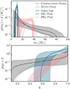 |
Fig. 3. Population distributions for primary mass (m1, top panel) and mass ratio (q, bottom panel) using the COMPACTNESS PEAKS model for BBH mergers scaled by the fraction of events in the BHL Peak (blue), BHH Peak (pink), and POWER LAW (black) components. The solid curve is the median of the distribution and the shaded regions represent the 90% credible interval. The dashed line represents the median of the distribution for the MULTI PEAK model, which has the same mass ratio distribution for all components. |
We also find shifts in the fraction of BBHs in each component with events in the power-law component moving to the peaked components when comparing the COMPACTNESS PEAKS and MULTI PEAK models, as shown in Figure 4. The 90% credible intervals for the fraction of binaries in each component are  ,
,  , and
, and  for COMPACTNESS PEAKS and
  ,
,  , and
, and  for MULTI PEAK.
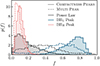 |
Fig. 4. Fraction of binary BHs in the BHL Peak (blue), BHH Peak (pink), and POWER LAW (black) components using the COMPACTNESS PEAKS (solid lines) and MULTI PEAK (dashed lines) model analyses. |
In Figure 5, we consider the slope index, β, of the mass ratio distribution for each component. We find that the power-law component has no preference for q ∼ 1, but rather a uniform distribution, whereas the BHH Peak component strongly prefers more positive slopes (i.e. q ∼ 1), which is consistent with findings from Li et al. (2022, 2024a). The BHL Peak component appears to return the prior for β. This result is because the truncation in the mass-ratio distribution – due to the strict pairing of the peaks in m1 and m2 – is driving its shape. However, if we relax this restriction by letting
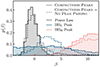 |
Fig. 5. Slope index of the mass-ratio distribution of the BHL Peak (blue), BHH Peak (pink), and POWER LAW (black) components using the COMPACTNESS PEAKS (solid lines) and COMPACTNESS PEAKS + NO PEAK PAIRING (dashed lines), which has relaxed conditions on the pairing of m1 and m2. |
 (12)
(12)
and
 (13)
(13)
such that m2 is not confined to be within the component defined in m1 space, we find the BHL Peak components also prefer positive slopes for the mass-ratio distribution. This analysis also reveals a preference for values of q ∼ 1 for the peak components. This model variation is hereafter referred to as COMPACTNESS PEAKS + NO PEAK PAIRING. We also find that this model, with a relaxed condition on the mass-ratio model, is slightly more preferred than the COMPACTNESS PEAKS model, by log10ℬ = 0.3. While this preference suggests that the strict pairing of m1 and m2 in the peaked component regions (as illustrated in Equation 7) may not be necessary to describe the population at present, the preference of q ∼ 1 in the peaked components still remains and can be accounted for by the positive values of β, as shown in Figure 5. The preference for an equal mass ratio in these peaked regions is also supported by findings in Sadiq et al. (2024).
Figure 6 shows that the populations in the power-law and compactness peaks have different spin properties, where the peaked components have lower spins than the power-law component and are generally more aligned with respect to the orbital angular momentum. However, the result for the power-law component is somewhat prior driven (see Figure B.2) given the small fraction of BBHs in the power-law component of namely f ∼ 0.15. We also observe that the power-law component has accounted for events with higher spins and very low spins, with reduced support for these values in the peaked distributions in comparison to the MULTI PEAK model.
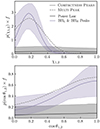 |
Fig. 6. Population distributions for spin magnitude (χ, top panel) and spin orientation (cos θ, bottom panel) using the COMPACTNESS PEAKS model for BBHs mergers scaled by the fraction of events in the BHL and BHH PEAKS (purple), and POWER LAW (black) components. The solid curve is the median of the distribution and the shaded regions represent the 90% credible interval. The dashed line represents the median of the distribution obtained from the MULTI PEAK model analysis, which has the same spin distribution for all components. |
We also considered a few variations of the COMPACTNESS PEAKS and COMPACTNESS PEAKS + NO PEAK PAIRING without separate spin distributions (i.e. the same values for the spin parameters μχ, σχ, σt, ζ) for the power law and peak populations (Table 2). We find that support for these models is significantly driven by allowing for separate spin populations (log10ℬ ∼ 1 − 3). Interestingly, the degree of increase in model support with and without separate spin populations varies depending on the mass-ratio distribution of the model. This result suggests that mass and spin are not strictly independent parameters and this may be a consequence of the χeff − q correlation (Callister et al. 2021; Adamcewicz & Thrane 2022).
4. Discussion
Motivated by the hypothesis presented in Schneider et al. (2023) for the presence of a gap in the component-mass spectrum of merging BBHs, we analysed the events in Abbott et al. (2023b) using a population designed to capture the structure of the compactness peaks and the degree of pairing of the peak regions in m1 and m2. We also explored whether there is a subpopulation of events that have properties that are different from those of the BBHs we expect from binary stripped stars (e.g. formed via dynamical evolution).
We find that there is a preference for the lower-mass peak to drop off sharply at  and the upper-mass peak to turn on at
  (90% credible intervals). The locations of the possible edges of the peaks are consistent with predictions from Schneider et al. (2023), with a possible gap, but there is no clear evidence for a gap-like feature given that the posteriors of the edges of the peaks overlap. If we consider the case where there is no power-law component to sweep up the ‘pollutants’ (i.e. only the compactness peaks), support for a gap-like structure decreases, with the edges at
  and
and  (90% credible intervals).
We also find mild support for the peaked populations to have a different spin distribution to the population defined by the power-law component. This result may hint at the possibility that the power-law component events were formed via alternative pathways to that leading to binary stripped stars in isolation, with 4 − 44% of binaries in the power-law component compared to 56 − 96% in the peaked components, and the majority of binaries, 48 − 87%, being found in the low-mass peak (90% credible intervals). However, more events are needed to constrain these results. With events from the fourth LVK observing run (O4), which includes the KAGRA (Akutsu et al. 2019) observatory in the gravitational-wave network, we expect our sample size to grow by a factor of about 3 (Abbott et al. 2018; Iacovelli et al. 2022; Kiendrebeogo et al. 2023). This increase may help us to constrain the parameters defining the power-law component and the edges of the compactness peaks.
Recent studies with a focus on looking for hierarchical mergers in the population find evidence that the spin properties of observed BBHs change at m ≈ 40 − 50 M⊙ (e.g. Li et al. 2024b; Antonini et al. 2025; Pierra et al. 2024). In our work, we find that the upper mass compactness peak turns off at m ≈ 37 − 42 M⊙, which appears to be consistent with these findings. This result is not driven by the spin information for each component. When fixing each mass component to have the same spin distribution, the turn off is at m ≈ 37 − 41 M⊙. However, there is a preference for the power-law component to have a different spin distribution to the compactness peak populations. Given that χeff is a more tightly constrained parameter, it would be interesting to investigate the variation of χeff across these different populations and how it compares to our analysis with component spins.
In the later stages of the preparation of this paper, the authors became aware of a similar study exploring the proposed gap in the component masses (Adamcewicz et al. 2024). In their work, the authors aim to answer the question of whether there is a lack of BHs within m ≈ 10 − 15 M⊙. To do this, they directly model a dip-like feature in the component-mass distribution using a notch filter – the same as that proposed in Farah et al. (2022) – to explore the gap between the masses of neutron stars and BHs. Similar to our model, they also use two peaks that surround this gap. They do not find evidence for a dip-like feature in the distribution. Considering there are events ‘polluting the gap’, and given the mass posterior uncertainties are generally larger than the width of the gap, this result is not unexpected. The authors also conclude that the dip-like feature will likely not reveal itself with an increased catalogue of events from O4. In our work, we aim to answer a slightly different question, which pertains to whether or not there is a lack of BHs within m ≈ 10 − 15 M⊙ given the expectation of pollution in this region from BBHs formed via other channels. These two approaches lead to slightly different conclusions, with support for the edges of the possible gap-like feature more pronounced in our work, and strong support for our Schneider et al. (2023) inspired model (log10ℬ = 4.63). However, both studies conclude that there is no clear evidence for a gap-like feature in component mass.
In addition to this, the requirement of q = m2/m1 ≤ 1 may also be impacting our results. This prior restriction results in the skewed posteriors we observe for some events, where the mass ratio is close to unity. This effect is particularly evident in the events with masses of < 15 M⊙, where slight shifts in mass lead to much more unequal mass ratios. To mitigate this, future analyses extending this prior range to the individual events may help resolve the structure and edges of the compactness peaks. Extending this, it may be interesting to study this same population with a spin-sorting approach rather than a mass-sorting approach, where the objects are ordered according to their spin magnitude rather than their mass. This approach can also constrain spin information and has the greatest impact for events of q ∼ 1 (e.g. Biscoveanu et al. 2021)
We highlight that in recent years, there has been a move towards data-driven models (e.g. Edelman et al. 2022; Tiwari 2023; Callister & Farr 2024) for the analysis of compact binary populations. These data-driven methods are valuable for finding structure in distribution without strong assumptions on the shape of the underlying distribution. However, astrophysically informed parametric models provide a clear method for astrophysical interpretations of the features observed and are ideal for model comparison. In this data-rich era, both data-driven and phenomenological models are needed: one to identify the possible new structure and one to interpret the astrophysical implications for the features we observe.
Data availability
Supplementary material including analysis inputs, posterior samples and additional plots are available here github.com/shanikagalaudage/bbhcompactnesspeaks
See Figure 6 in Schneider et al. (2023) for an illustration of how physical processes shift the edges of the 10 − 15 M⊙ gap in component mass.
See Thrane & Talbot (2019) for a detailed review of parameter estimation and hierarchical inference in gravitational wave astronomy; the methods used for our analysis are equivalent to those described in their Section 5.
We use a variation of the MULTI PEAK model without smoothing (δm = 0) and different priors on the parameters. For details of this model, see Section B.4 in Abbott et al. (2021b); the priors used are provided in Table A.2. We use the same spin and redshift model as those used for COMPACTNESS PEAKS, but the same spin distribution is used for all components.
Acknowledgments
We thank Giuliano Iorio and the anonymous reviewer for their helpful comments on this work. Galaudage and Lamberts are supported by the ANR COSMERGE project, grant ANR-20-CE31-001 of the French Agence Nationale de la Recherche. The authors are grateful for computational resources provided by the LIGO Laboratory and supported by National Science Foundation Grants PHY-0757058 and PHY-0823459. This material is based upon work supported by NSF’s LIGO Laboratory which is a major facility fully funded by the National Science Foundation
References
- Aasi, J., Abbott, B. P., Abbott, R., et al. 2015, CQG, 32, 074001 [Google Scholar]
- Abbott, B. P., Abbott, R., Abbott, T. D., et al. 2016a, PRX, 6, 041015; Erratum: PRX 8, 039903 (2018) [Google Scholar]
- Abbott, B. P., Abbott, R., Abbott, T. D., et al. 2016b, PRL, 116, 241103 [NASA ADS] [CrossRef] [Google Scholar]
- Abbott, B. P., Abbott, R., Abbott, T. D., et al. 2017, ApJ, 851, L35 [Google Scholar]
- Abbott, B. P., Abbott, R., Abbott, T. D., et al. 2018, Liv. Rev. Rel., 21, 3 [Google Scholar]
- Abbott, R., Abbott, T. D., Abraham, S., et al. 2020, PRD, 102, 043015 [NASA ADS] [CrossRef] [Google Scholar]
- Abbott, R., Abbott, T. D., Abraham, S., et al. 2021a, PRX, 11, 021053 [Google Scholar]
- Abbott, R., Abbott, T. D., Abraham, S., et al. 2021b, ApJ, 913, L7 [NASA ADS] [CrossRef] [Google Scholar]
- Abbott, R., Abbott, T. D., Acernese, F., et al. 2023a, PRX, 13, 041039 [Google Scholar]
- Abbott, R., Abbott, T. D., Acernese, F., et al. 2023b, PRX, 13, 011048 [Google Scholar]
- Acernese, F., Agathos, M., Agatsuma, K., et al. 2015, CQG, 32, 024001 [NASA ADS] [CrossRef] [Google Scholar]
- Adamcewicz, C., & Thrane, E. 2022, MNRAS, 517, 3928 [NASA ADS] [CrossRef] [Google Scholar]
- Adamcewicz, C., Lasky, P. D., Thrane, E., & Mandel, I. 2024, ApJ, 975, 253 [Google Scholar]
- Ajith, P., Hannam, M., Husa, S., et al. 2011, PRL, 106, 241101 [NASA ADS] [CrossRef] [Google Scholar]
- Akutsu, T., Ando, M., Arai, K., et al. 2019, Nat. Astron., 3, 35 [NASA ADS] [CrossRef] [Google Scholar]
- Antonelli, A., Kritos, K., Ng, K. K. Y., Cotesta, R., & Berti, E. 2023, PRD, 108, 084044 [NASA ADS] [CrossRef] [Google Scholar]
- Antonini, F., Gieles, M., Dosopoulou, F., & Chattopadhyay, D. 2023, MNRAS, 522, 466 [NASA ADS] [CrossRef] [Google Scholar]
- Antonini, F., Romero-Shaw, I. M., & Callister, T. 2025, Phys. Rev. Lett., 134, 011401 [CrossRef] [Google Scholar]
- Ashton, G., Hübner, M., Lasky, P. D., et al. 2019, ApJS, 241, 27 [NASA ADS] [CrossRef] [Google Scholar]
- Bavera, S. S., Fragos, T., Qin, Y., et al. 2020, A&A, 635, A97 [NASA ADS] [CrossRef] [EDP Sciences] [Google Scholar]
- Belczynski, K., Bulik, T., Fryer, C. L., et al. 2010, ApJ, 714, 1217 [NASA ADS] [CrossRef] [Google Scholar]
- Biscoveanu, S., Isi, M., Vitale, S., & Varma, V. 2021, PRL, 126, 171103 [NASA ADS] [CrossRef] [Google Scholar]
- Blanchet, L., Damour, T., Iyer, B. R., Will, C. M., & Wiseman, A. G. 1995, PRL, 74, 3515 [NASA ADS] [CrossRef] [Google Scholar]
- Broekgaarden, F. S., Berger, E., Stevenson, S., et al. 2022, MNRAS, 516, 5737 [NASA ADS] [CrossRef] [Google Scholar]
- Burrows, A., Vartanyan, D., & Wang, T. 2023, ApJ, 957, 68 [NASA ADS] [CrossRef] [Google Scholar]
- Burrows, A., Wang, T., & Vartanyan, D. 2024, ApJ, 964, L16 [NASA ADS] [CrossRef] [Google Scholar]
- Callister, T. A., & Farr, W. M. 2024, PRX, 14, 021005 [Google Scholar]
- Callister, T. A., Haster, C.-J., Ng, K. K. Y., Vitale, S., & Farr, W. M. 2021, ApJ, 922, L5 [NASA ADS] [CrossRef] [Google Scholar]
- Chatterjee, S., Rodriguez, C. L., Kalogera, V., & Rasio, F. A. 2017, ApJ, 836, L26 [NASA ADS] [CrossRef] [Google Scholar]
- Chieffi, A., & Limongi, M. 2020, ApJ, 890, 1 [NASA ADS] [CrossRef] [Google Scholar]
- Costa, G., Bressan, A., Mapelli, M., et al. 2021, MNRAS, 501, 4514 [NASA ADS] [CrossRef] [Google Scholar]
- Croon, D., & Sakstein, J. 2023, arXiv e-prints [arXiv:2312.13459] [Google Scholar]
- Doctor, Z., Wysocki, D., O’Shaughnessy, R., Holz, D. E., & Farr, B. 2020, ApJ, 893, 35 [NASA ADS] [CrossRef] [Google Scholar]
- Edelman, B., Doctor, Z., Godfrey, J., & Farr, B. 2022, ApJ, 924, 101 [NASA ADS] [CrossRef] [Google Scholar]
- Essick, R., & Farr, W. 2022, arXiv e-prints [arXiv:2204.00461] [Google Scholar]
- Farag, E., Renzo, M., Farmer, R., Chidester, M. T., & Timmes, F. X. 2022, ApJ, 937, 112 [NASA ADS] [CrossRef] [Google Scholar]
- Farah, A. M., Fishbach, M., Essick, R., Holz, D. E., & Galaudage, S. 2022, ApJ, 931, 108 [NASA ADS] [CrossRef] [Google Scholar]
- Farah, A. M., Edelman, B., Zevin, M., et al. 2023, ApJ, 955, 107 [NASA ADS] [CrossRef] [Google Scholar]
- Farmer, R., Renzo, M., de Mink, S. E., Marchant, P., & Justham, S. 2019, ApJ, 887, 53 [Google Scholar]
- Farmer, R., Renzo, M., de Mink, S., Fishbach, M., & Justham, S. 2020, ApJ, 902, L36 [CrossRef] [Google Scholar]
- Finn, L. S., & Chernoff, D. F. 1993, PRD, 47, 2198 [NASA ADS] [CrossRef] [Google Scholar]
- Fishbach, M., Holz, D. E., & Farr, W. M. 2018, ApJ, 863, L41 [NASA ADS] [CrossRef] [Google Scholar]
- Gerosa, D., & Berti, E. 2017, PRD, 95, 124046 [NASA ADS] [CrossRef] [Google Scholar]
- Gerosa, D., Berti, E., O’Shaughnessy, R., et al. 2018, PRD, 98, 084036 [NASA ADS] [CrossRef] [Google Scholar]
- Gerosa, D., Vitale, S., & Berti, E. 2020, PRL, 125, 101103 [NASA ADS] [CrossRef] [Google Scholar]
- Giacobbo, N., & Mapelli, M. 2018, MNRAS, 480, 2011 [Google Scholar]
- Golomb, J., Isi, M., & Farr, W. 2024, ApJ, 976, 121 [NASA ADS] [CrossRef] [Google Scholar]
- Hannam, M., Schmidt, P., Bohé, A., et al. 2014, PRL, 113, 151101 [NASA ADS] [CrossRef] [Google Scholar]
- Heger, A., & Woosley, S. E. 2002, ApJ, 567, 532 [Google Scholar]
- Hendriks, D. D., van Son, L. A. C., Renzo, M., Izzard, R. G., & Farmer, R. 2023, MNRAS, 526, 4130 [NASA ADS] [CrossRef] [Google Scholar]
- Iacovelli, F., Mancarella, M., Foffa, S., & Maggiore, M. 2022, ApJ, 941, 208 [NASA ADS] [CrossRef] [Google Scholar]
- Iorio, G., Mapelli, M., Costa, G., et al. 2023, MNRAS, 524, 426 [NASA ADS] [CrossRef] [Google Scholar]
- Kiendrebeogo, R. W., Farah, A. M., Foley, E. M., et al. 2023, ApJ, 958, 158 [NASA ADS] [CrossRef] [Google Scholar]
- Kruckow, M. U., Tauris, T. M., Langer, N., Kramer, M., & Izzard, R. G. 2018, MNRAS, 481, 1908 [CrossRef] [Google Scholar]
- Li, Y.-J., Wang, Y.-Z., Tang, S.-P., et al. 2022, ApJ, 933, L14 [NASA ADS] [CrossRef] [Google Scholar]
- Li, Y. J., Tang, S. P., Gao, S. J., Wu, D. C., & Wang, Y. Z. 2024a, ApJ, 977, 67 [NASA ADS] [CrossRef] [Google Scholar]
- Li, Y.-J., Wang, Y.-Z., Tang, S.-P., & Fan, Y.-Z. 2024b, PRL, 133, 051401 [NASA ADS] [CrossRef] [Google Scholar]
- Liu, B., & Lai, D. 2021, MNRAS, 502, 2049 [NASA ADS] [CrossRef] [Google Scholar]
- Mandel, I., & Broekgaarden, F. S. 2022, Liv. Rev. Rel., 25, 1 [CrossRef] [Google Scholar]
- Mandel, I., & Farmer, A. 2022, Phys. Rept., 955, 1 [NASA ADS] [CrossRef] [Google Scholar]
- Mandel, I., & O’Shaughnessy, R. 2010, CQG, 27, 114007 [Google Scholar]
- Mapelli, M. 2020, Proc. Int. Sch. Phys. Fermi, 200, 87 [Google Scholar]
- Mapelli, M., Spera, M., Montanari, E., et al. 2020, ApJ, 888, 76 [NASA ADS] [CrossRef] [Google Scholar]
- O’Connor, E., & Ott, C. D. 2011, ApJ, 730, 70 [Google Scholar]
- O’Shaughnessy, R., Gerosa, D., & Wysocki, D. 2017, PRL, 119, 011101 [CrossRef] [Google Scholar]
- Patton, R. A., & Sukhbold, T. 2020, MNRAS, 499, 2803 [NASA ADS] [CrossRef] [Google Scholar]
- Pierra, G., Mastrogiovanni, S., & Perriès, S. 2024, arXiv e-prints [arXiv:2406.01679] [Google Scholar]
- Poisson, E., & Will, C. M. 1995, PRD, 52, 848 [NASA ADS] [CrossRef] [Google Scholar]
- Rahman, N., Janka, H.-T., Stockinger, G., & Woosley, S. 2022, MNRAS, 512, 4503 [NASA ADS] [CrossRef] [Google Scholar]
- Rodriguez, C. L., Zevin, M., Pankow, C., Kalogera, V., & Rasio, F. A. 2016, ApJ, 832, L2 [NASA ADS] [CrossRef] [Google Scholar]
- Rodriguez, C. L., Amaro-Seoane, P., Chatterjee, S., & Rasio, F. A. 2018, PRL, 120, 151101 [NASA ADS] [CrossRef] [Google Scholar]
- Romero-Shaw, I. M., Talbot, C., Biscoveanu, S., et al. 2020, MNRAS, 499, 3295 [NASA ADS] [CrossRef] [Google Scholar]
- Sadiq, J., Dent, T., & Wysocki, D. 2022, PRD, 105, 123014 [NASA ADS] [CrossRef] [Google Scholar]
- Sadiq, J., Dent, T., & Gieles, M. 2024, ApJ, 960, 65 [NASA ADS] [CrossRef] [Google Scholar]
- Safarzadeh, M., & Hotokezaka, K. 2020, ApJ, 897, L7 [NASA ADS] [CrossRef] [Google Scholar]
- Santamaria, L., Ohme, F., Ajith, P., et al. 2010, PRD, 82, 064016 [NASA ADS] [CrossRef] [Google Scholar]
- Schmidt, P., Ohme, F., & Hannam, M. 2015, PRD, 91, 024043 [NASA ADS] [CrossRef] [Google Scholar]
- Schneider, F. R. N., Podsiadlowski, P., & Müller, B. 2021, A&A, 645, A5 [NASA ADS] [CrossRef] [EDP Sciences] [Google Scholar]
- Schneider, F. R. N., Podsiadlowski, P., & Laplace, E. 2023, ApJ, 950, L9 [NASA ADS] [CrossRef] [Google Scholar]
- Speagle, J. S. 2020, MNRAS, 493, 3132 [Google Scholar]
- Spera, M., Mapelli, M., & Bressan, A. 2015, MNRAS, 451, 4086 [NASA ADS] [CrossRef] [Google Scholar]
- Spera, M., Trani, A. A., & Mencagli, M. 2022, Galaxies, 10, 76 [NASA ADS] [CrossRef] [Google Scholar]
- Stevenson, S., Berry, C. P. L., & Mandel, I. 2017, MNRAS, 471, 2801 [NASA ADS] [CrossRef] [Google Scholar]
- Stevenson, S., Sampson, M., Powell, J., et al. 2019, ApJ, 882, 121 [Google Scholar]
- Sukhbold, T., & Woosley, S. 2014, ApJ, 783, 10 [NASA ADS] [CrossRef] [Google Scholar]
- Talbot, C., & Thrane, E. 2017, PRD, 96, 023012 [NASA ADS] [CrossRef] [Google Scholar]
- Talbot, C., & Thrane, E. 2018, ApJ, 856, 173 [NASA ADS] [CrossRef] [Google Scholar]
- Talbot, C., Smith, R., Thrane, E., & Poole, G. B. 2019, PRD, 100, 043030 [NASA ADS] [CrossRef] [Google Scholar]
- Temaj, D., Schneider, F. R. N., Laplace, E., Wei, D., & Podsiadlowski, P. 2024, A&A, 682, A123 [NASA ADS] [CrossRef] [EDP Sciences] [Google Scholar]
- Thrane, E., & Talbot, C. 2019, PASA, 36, e010; Erratum: PASA 37, e036 (2020) [NASA ADS] [CrossRef] [Google Scholar]
- Tiwari, V. 2022, ApJ, 928, 155 [NASA ADS] [CrossRef] [Google Scholar]
- Tiwari, V. 2023, MNRAS, 527, 298 [NASA ADS] [CrossRef] [Google Scholar]
- Tiwari, V., & Fairhurst, S. 2021, ApJ, 913, L19 [CrossRef] [Google Scholar]
- van Son, L. A. C., de Mink, S. E., Renzo, M., et al. 2022, ApJ, 940, 184 [NASA ADS] [CrossRef] [Google Scholar]
- Vink, J. S., & de Koter, A. 2005, A&A, 442, 587 [NASA ADS] [CrossRef] [EDP Sciences] [Google Scholar]
- Wong, K. W. K., & Cranmer, M. 2022, in 39th International Conference on Machine Learning Conference [Google Scholar]
- Yang, Y., Bartos, I., Gayathri, V., et al. 2019, PRL, 123, 181101 [NASA ADS] [CrossRef] [Google Scholar]
- Zevin, M., Pankow, C., Rodriguez, C. L., et al. 2017, ApJ, 846, 82 [NASA ADS] [CrossRef] [Google Scholar]
- Zhang, R. C., Fragione, G., Kimball, C., & Kalogera, V. 2023, ApJ, 954, 23 [NASA ADS] [CrossRef] [Google Scholar]
Appendix A: Population model details
In this section we provide details about the population models described above in Section 2.2. We include a summary of the parameters for the COMPACTNESS PEAKS and MULTI PEAK models and the prior distribution used for each parameter in Tables A.1 and A.2 respectively. The prior distributions are indicated using abbreviations: for example, U(0, 1) translates to uniform on the interval (0, 1).
Summary of parameters in COMPACTNESS PEAKS population model.
Summary of parameters in MULTI PEAK model.
Appendix B: Hyperparameter posteriors
In this section we provide the hyperparameter posteriors for the parameters governing the peak components of the mass distribution (Figure B.1) and the spin parameters for the peaked and powerlaw components (Figure B.2).
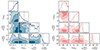 |
Fig. B.1. Mass hyperparameter posteriors of the peak components in the COMPACTNESS PEAKS model. Left panel: the lower mass (BHL) peak where μBHL is the mean of the peak, σBHL is the width of the peak and mminBHL and mmaxBHL are the minimum and maximum mass of the peak. Right panel: the upper mass (BHL) peak where μBHH is the mean of the peak, σBHH is the width of the peak and mminBHH and mmaxBHH are the minimum and maximum mass of the peak. The credible intervals on the 2D posterior distributions are at 1σ, 2σ and 3σ, using increasingly light shading. The intervals on the 1D posterior distributions are at 1σ. |
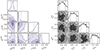 |
Fig. B.2. Spin hyperparameter posteriors of the COMPACTNESS PEAKS model, where μχ is the mean of the spin magnitude distribution, σχ is the width of the spin magnitude distribution, ζ is the fraction of BBHs in the subpopulation aligned with respect to the orbital angular momentum and σt is the width of the spin orientation distribution for the subpopulation aligned with respect to the orbital angular momentum for a given component. Left panel: The spin parameters paired with the BHL and BHH peaks Right panel: The spin parameters paired with the powerlaw (PL) component. The credible intervals on the 2D posterior distributions are at 1σ, 2σ and 3σ, using increasingly light shading. The intervals on the 1D posterior distributions are at 1σ. |
All Tables
All Figures
|
Fig. 1. Events in GWTC-3 with FAR < 1yr−1 sorted according to the chirp-mass peak in which they lie, assuming the Schneider et al. (2023) predictions regarding their classification and the locations of the gaps. Top panel: Chirp-mass posteriors showing the BHL + BHL (blue) and the BHH + BHH (pink). The grey shaded region represents the chirp-mass gap region (ℳ ≈ 10 − 12 M⊙). Bottom panel: Component-mass posteriors showing the BHL (blue) and the BHH (pink) BHs. The grey shaded region represents the expected component-mass gap region (m ≈ 10 − 15 M⊙). The vertical ticks illustrate the median of each posterior. |
| In the text | |
|
Fig. 2. Two-dimensional distributions of the mass ratio (q), effective inspiral spin (χeff), and effective precession spin (χp) of events polluting the m = 10 − 15 M⊙ gap (pink and blue shaded region; 90% credibility) and the median (pink and blue dots). The medians of the posteriors of the events outside the gap are also shown (black dots). Events polluting the gap (GW190412, GW151226, and GW200225), which may have formed via a channel different from isolated binary evolution, are highlighted with stars. |
| In the text | |
|
Fig. 3. Population distributions for primary mass (m1, top panel) and mass ratio (q, bottom panel) using the COMPACTNESS PEAKS model for BBH mergers scaled by the fraction of events in the BHL Peak (blue), BHH Peak (pink), and POWER LAW (black) components. The solid curve is the median of the distribution and the shaded regions represent the 90% credible interval. The dashed line represents the median of the distribution for the MULTI PEAK model, which has the same mass ratio distribution for all components. |
| In the text | |
|
Fig. 4. Fraction of binary BHs in the BHL Peak (blue), BHH Peak (pink), and POWER LAW (black) components using the COMPACTNESS PEAKS (solid lines) and MULTI PEAK (dashed lines) model analyses. |
| In the text | |
|
Fig. 5. Slope index of the mass-ratio distribution of the BHL Peak (blue), BHH Peak (pink), and POWER LAW (black) components using the COMPACTNESS PEAKS (solid lines) and COMPACTNESS PEAKS + NO PEAK PAIRING (dashed lines), which has relaxed conditions on the pairing of m1 and m2. |
| In the text | |
|
Fig. 6. Population distributions for spin magnitude (χ, top panel) and spin orientation (cos θ, bottom panel) using the COMPACTNESS PEAKS model for BBHs mergers scaled by the fraction of events in the BHL and BHH PEAKS (purple), and POWER LAW (black) components. The solid curve is the median of the distribution and the shaded regions represent the 90% credible interval. The dashed line represents the median of the distribution obtained from the MULTI PEAK model analysis, which has the same spin distribution for all components. |
| In the text | |
|
Fig. B.1. Mass hyperparameter posteriors of the peak components in the COMPACTNESS PEAKS model. Left panel: the lower mass (BHL) peak where μBHL is the mean of the peak, σBHL is the width of the peak and mminBHL and mmaxBHL are the minimum and maximum mass of the peak. Right panel: the upper mass (BHL) peak where μBHH is the mean of the peak, σBHH is the width of the peak and mminBHH and mmaxBHH are the minimum and maximum mass of the peak. The credible intervals on the 2D posterior distributions are at 1σ, 2σ and 3σ, using increasingly light shading. The intervals on the 1D posterior distributions are at 1σ. |
| In the text | |
|
Fig. B.2. Spin hyperparameter posteriors of the COMPACTNESS PEAKS model, where μχ is the mean of the spin magnitude distribution, σχ is the width of the spin magnitude distribution, ζ is the fraction of BBHs in the subpopulation aligned with respect to the orbital angular momentum and σt is the width of the spin orientation distribution for the subpopulation aligned with respect to the orbital angular momentum for a given component. Left panel: The spin parameters paired with the BHL and BHH peaks Right panel: The spin parameters paired with the powerlaw (PL) component. The credible intervals on the 2D posterior distributions are at 1σ, 2σ and 3σ, using increasingly light shading. The intervals on the 1D posterior distributions are at 1σ. |
| In the text | |
Current usage metrics show cumulative count of Article Views (full-text article views including HTML views, PDF and ePub downloads, according to the available data) and Abstracts Views on Vision4Press platform.
Data correspond to usage on the plateform after 2015. The current usage metrics is available 48-96 hours after online publication and is updated daily on week days.
Initial download of the metrics may take a while.