GWSim: Python package for creating mock GW samples for different astrophysical populations and cosmological models of binary black holes

Christos Karathanasis; Benoît Revenu; Suvodip Mukherjee; Federico Stachurski

doi:10.1051/0004-6361/202245216

Home

All issues

Volume 677 (September 2023)

A&A, 677 (2023) A124

Full HTML

Open Access

This article has an erratum: [https://doi.org/10.1051/0004-6361/202245216e]

Issue		A&A Volume 677, September 2023


Article Number		A124
Number of page(s)		18
Section		Numerical methods and codes
DOI		https://doi.org/10.1051/0004-6361/202245216
Published online		19 September 2023

A&A, 677, A124 (2023)

`GWSim`: Python package for creating mock GW samples for different astrophysical populations and cosmological models of binary black holes^★

Christos Karathanasis¹, Benoît Revenu²^,3, Suvodip Mukherjee⁴ and Federico Stachurski⁵

¹ Institut de Física d’Altes Energies (IFAE), Barcelona Institute of Science and Technology, Barcelona, Spain
e-mail: ckarathanasis@ifae.es
² Subatech, CNRS, Institut Mines-Telecom Atlantique, Nantes Université, 44000 Nantes, France
³ Université Paris Cité, CNRS, Astroparticule et Cosmologie, 75000 Paris, France
⁴ Department of Astronomy & Astrophysics, Tata Institute of Fundamental Research, 1, Homi Bhabha Road, Colaba, Mumbai 400005, India
e-mail: suvodip@tifr.res.in
⁵ Institute of Gravitational Research (IGR), University of Glasgow, Glasgow, UK

Received: 14 October 2022
Accepted: 21 June 2023

Abstract

Precision cosmology with gravitational wave (GW) sources requires a deeper understanding of the interplay between GW source population and cosmological parameters governing the dynamics of the Universe. With the swift increase in GW detections, it is necessary to develop a tool for exploring many aspects of cosmology and fundamental physics; this tools allows to simulate GW mock samples for several populations and cosmological models. We have developed a new code called GWSim, which allows us to make a large sample of GW mock events from a broad range of configurations, while varying the cosmology, the merger rate, and the GW source parameters (i.e. mass and spin distributions in particular) for a given network of GW detectors. A large sample of simulated mock GW events will be useful for improving our understanding of the statistical properties of the distribution of GW sources, as long as it is detectable for a given detector noise and an astrophysical and cosmological model. It will also be useful to compare simulated samples with the observed distribution of the GW sources from data and infer the underlying population of the GW source parameters and cosmology. We restricted the cosmology to spatially flat universes, including models with varying dark energy equation of state. The GWSim code provides each mock event with a position in the sky and a redshift; these values can be those of random host galaxies coming from an isotropic and homogeneous simulated Universe or a user-supplied galaxy catalog. We used realistic detector configurations of the LIGO and Virgo network of detectors to demonstrate the performance of this code for the latest observation runs and the upcoming observation run.

Key words: gravitational waves / methods: numerical

^★

GWSim is publicly available at: https://git.ligo.org/benoit.revenu/gwsim

© The Authors 2023

Open Access article, published by EDP Sciences, under the terms of the Creative Commons Attribution License (https://creativecommons.org/licenses/by/4.0), which permits unrestricted use, distribution, and reproduction in any medium, provided the original work is properly cited.

This article is published in open access under the Subscribe to Open model. Subscribe to A&A to support open access publication.

1 Introduction

The detection of the gravitational wave (GWs) sources by the LIGO-Virgo-KAGRA collaboration (Gregory 2010; Aso et al. 2013; Acernese et al. 2014; The LIGO Scientific Collaboration 2015; Abbott et al. 2016, 2018, 2019a, 2021c; Martynov et al. 2016; The LIGO Scientific Collaboration et al. 2021; The LIGO Scientific Collaboration & the Virgo Collaboration 2021; Tse et al. 2019; Akutsu et al. 2021) has opened up an era of GW astronomy capable of bringing a plethora of scientific discoveries in astrophysics, cosmology, and fundamental physics. With the fourth campaign of data taking O4 that began on May 24, 2023, the expected event rate will rise to some BBHs per day (i.e. more than four times the GW event rate during O3b). Such discoveries will require an understanding of different sources of statistical and systematic uncertainties as well as the interplay between the astrophysical population of GW sources, the cosmological models, the fundamental physics, and searches beyond the standard model (Abbott et al. 2019b, Abbott et al. 2021a, 2023a,b). To understand these, we need realistic simulations of GW events for different astrophysical populations and cosmological models, including realistic detector sensitivities.

We used GWSim to simulate a sample of mock GW sources for different (i) mass, (ii) spin, and (iii) merger rate models, as well as for the flat Λ cold dark matter (ΛCDM) and flat w₀− w_aCDM cosmological models. The code assigns host galaxies to GW events in two cases: assuming a constant in comoving volume distribution of galaxies or using a simulated galaxy catalog, such as MICECATv2 (Fosalba et al. 2014, 2015; Crocce et al. 2015). The code also considers different detector sensitivities and observation periods. Then, the Bilby (Ashton et al. 2019) pipeline is used to generate the actual GW strains corresponding to these GW events and perform parameter estimation to finally obtain mock GW samples. Having access to these sets of samples allows us to estimate the performances of the analysis algorithms. For one given GW event, its associated samples consist of a list of values obtained by a Markov chain Monte Carlo (MCMC) algorithm of all the parameters describing the binary system; in particular, the luminosity distance of the source, the masses of the two black holes, and their spins. We applied this simulation code GWSim to generate mock sources with the detector sensitivity of the fourth observation run O4 of LIGO-Virgo-KAGRA collaboration and we came up with a forecast for the measurability of the astrophysical population parameters and Hubble constant. We find that GWSim will be useful to generate mock samples for different future detector sensitivities as well as varied astrophysical populations and cosmological parameters.

The paper is structured as follows. In Sect. 2, we describe different models included in the current version of GWSim. In Sects. 3 and 4, we describe the structure of the code and validated different setups.

Finally, in Sect. 5, we discuss the use and future developments of this code.

2 Models of cosmology and GW sources astrophysical population

Making inferences on the cosmological results using binary black holes (BBHs) requires an understanding of the dependencies on the astrophysical source parameters for different techniques such as statistical host identification (Schutz 1986; MacLeod & Hogan 2008; Del Pozzo 2012; Arabsalmani et al. 2013; Gray et al. 2020; Fishbach et al. 2019; Abbott et al. 2020, 2021a; Soares-Santos et al. 2019; Finke et al. 2021; Palmese et al. 2023), cross-correlation techniques after taking into account GW source population uncertainty (Oguri 2016; Mukherjee & Wandelt 2018; Mukherjee et al. 2020, 2021a,b, 2022; Calore et al. 2020; Bera et al. 2020; Scelfo et al. 2020, 2022; Cañas-Herrera et al. 2021; Cigarrán Díaz & Mukherjee 2022), or BBH mass-distribution (Taylor et al. 2012; Farr et al. 2019; Mastrogiovanni et al. 2021; You et al. 2021; Mancarella et al. 2022; Mukherjee 2022; Leyde et al. 2022; Ezquiaga & Holz 2022).

Here, we describe the cosmological models that can be used in GWSim and the models describing the population of BBH mergers (merger rates, mass distributions, and spin distributions).

2.1 Cosmological models

The code considers only the cosmological models with spatial curvature zero (flat) and for three scenarios namely, ΛCDM, w₀CDM, which takes into account variation of the dark energy equation of state without redshift dependence, and w₀−w_aCDM, which takes into account variation of the dark energy equation of state with redshift dependence (Chevallier & Polarski 2001; Linder 2003). In Table 1, we present these models. For a particular choice of the cosmological parameters, the code computes the luminosity distances D_L(z_m) to the merger situated at a redshift z_m using $D_{L} (z_{m}) = \frac{c (1 + z_{m})}{H_{0}} \int_{0}^{z_{m}} \frac{d z}{E (z)},$ ${D_{\rm{L}}}\,\left( {{z_{\rm{m}}}} \right) = {{c\left( {1 + z{ & _{\rm{m}}}} \right)} \over {{H_0}}}\,\,\int_0^{z{ & _{\rm{m}}}} {{{{\rm{d}}z} \over {E\left( z \right)}}} ,$ (1)

with E²(z) = Ω_m(l + z)³ + Ω_DE exp $[\int_{0}^{z} dln (1 + z^{'}) (1 + ω (z^{'}))]$ $\left[ {\int_0^z {{\rm{dln}}} \left( {1 + z'} \right)\left( {1 + \omega \left( {z'} \right)} \right)} \right]$ .

In the part of the code used for assigning the redshift to the GW sources from a galaxy catalog, we can calculate the luminosity distance to the source for different cosmological models. Although this part of the code can be used to infer the cosmological parameters using the luminosity distance, it cannot be used to estimate the variation of cross-correlation between the GW sources and galaxies for different cosmological parameters. To explore the cross-correlation signal, this can only be done in this way for the fiducial cosmological values considered in MICECATv2 simulations.

2.2 Merger rate models of the compact objects

We considered three scenarios for the merger rate of the binary compact objects: (a) constant merger rate, (b) phenomenological merger rate, and (c) delay-time model. The models are described in Table 2 and their parameters can be seen in Table 3.

The first scenario with a constant merger rate model is a model with a single parameter, R₀, which corresponds to a scenario with no redshift evolution. The second scenario of the model considers a merger rate varying with the redshift; it uses four phenomenological parameters (γ, κ, R₀, z_p) (Madau & Dickinson 2014): $R (z) = R_{0} {(1 + z)}^{γ} \frac{1 + {(1 + z_{p})}^{- (γ + κ)}}{1 + {(\frac{1 + z}{1 + z_{p}})}^{γ + κ}} .$ $R\left( z \right) = {R_0}\,{\left( {1 + z} \right)^\gamma }\,{{1 + {{\left( {1 + {z_{\rm{p}}}} \right)}^{ - \left( {\gamma + \kappa } \right)}}} \over {1 + {{\left( {{{1 + z} \over {1 + {z_{\rm{p}}}}}} \right)}^{\gamma + \kappa }}}}.$ (2)

The third model considered is driven by physics and that models the merger rate in terms of the delay time distribution denoted as t_d (O’Shaughnessy et al. 2010; Banerjee et al. 2010; Dominik et al. 2012, 2015; Mandel & de Mink 2016; Lamberts et al. 2016; Cao et al. 2018; Elbert et al. 2018; Eldridge et al. 2019; Vitale et al. 2019; du Buisson et al. 2020; Santoliquido et al. 2021). The time delay is the elapsed time between the formation of the stars (which later will become black holes) and the merging of the black holes. Currently, constraints on t_d are weak from individual events (Fishbach & Kalogera 2021; Karathanasis et al. 2023) and the stochastic GW background (Mukherjee & Silk 2021). In the future, by combing the properties of emission line galaxies with GW sources, a better measurement of the delay time is possible (Mukherjee & Dizgah 2022). The time delay is not the same value for all binary black holes, rather, it follows a distribution of P_t: $P_{t} (t_{d} | t_{d}^{\min}, t_{d}^{\max}, d) \propto {\begin{array}{l} {(t_{d})}^{- d} & , for t_{d}^{\min} < t_{d} < t_{d}^{\max} \\ 0 & otherwise \end{array} .$ ${P_t}\left( {\left. {{t_{\rm{d}}}} \right|t_{\rm{d}}^{\min },t_{\rm{d}}^{\max },{\rm{d}}} \right)\, \propto \,\,\left\{ {\matrix{ {{{\left( {{t_{\rm{d}}}} \right)}^{ - d}}} \hfill & {,\,{\rm{for}}\,t_{\rm{d}}^{\min }\, > {t_{\rm{d}}} & t_{\rm{d}}^{\max }} \hfill \cr 0 \hfill & {{\rm{otherwise}}} \hfill \cr } } \right..$ (3)

For a star to become a black hole only a few Myr are required, but for a black hole to find another companion, form a binary, and merge a significant amount of time is needed (on the order of Gyr). This model assumes a star formation rate and different power law forms of the probability distribution of the delay time P_t ( $t_{d} | t_{d}^{\min}$ $\left. {{t_{\rm{d}}}} \right|t_{\rm{d}}^{\min }$ , $t_{d}^{\max}$ $t_{\rm{d}}^{\max }$ , d) (Mukherjee 2022; Karathanasis et al. 2023). This model has four parameters (d, $t_{d}^{\min}$ $t_{\rm{d}}^{\min }$ , α_Z, γ_Z) as described in Table 3 and the corresponding merger rate at redshift, z, can be expressed as: $R_{TD} (z) = R_{0} \frac{\int_{z}^{\infty} P_{t} (t_{d} | t_{d}^{\min}, t_{d}^{\max}, d) R_{SFR} (z_{f}) \frac{d t}{d z_{f}} d z_{f}}{\int_{z}^{\infty} P_{t} (t_{d} | t_{d}^{\min}, t_{d}^{\max}, d) R_{SFR} (z_{f}) \frac{d t}{d z_{f}} d z_{f}}$ ${R_{{\rm{TD}}}}\left( z \right) = {R_0}{{\int_z^\infty {{P_t}\,\left( {\left. {{t_{\rm{d}}}} \right|t_{\rm{d}}^{\min },t_{\rm{d}}^{\max },d} \right){R_{{\rm{SFR}}}}\,\left( {{z_{\rm{f}}}} \right){{{\rm{d}}t} \over {{\rm{d}}{z_{\rm{f}}}}}{\rm{d}}{z_{\rm{f}}}} } \over {\int_z^\infty {{P_t}\,\left( {\left. {{t_{\rm{d}}}} \right|t_{\rm{d}}^{\min },t_{\rm{d}}^{\max },d} \right){R_{{\rm{SFR}}}}\,\left( {{z_{\rm{f}}}} \right){{{\rm{d}}t} \over {{\rm{d}}{z_{\rm{f}}}}}{\rm{d}}{z_{\rm{f}}}} }}$ (4)

where R_SFR is defined as (Madau & Dickinson 2014) $R_{SFR} (z) \propto \frac{{(1 + z)}^{2.7}}{1 + {[(1 + z) / 2.9]}^{5.6}} .$ ${R_{{\rm{SFR}}}}\left( z \right) \propto {{{{\left( {1 + z} \right)}^{2.7}}} \over {1 + {{\left[ {{{\left( {1 + z} \right)} \mathord{\left/ {\vphantom {{\left( {1 + z} \right)} {2.9}}} \right. \kern-\nulldelimiterspace} {2.9}}} \right]}^{5.6}}}}.$ (5)

For each of these merger rates R(z), the number of coalescing events per unit redshift per unit observation time is calculated using $\frac{d N_{GW}}{d z d t} = \frac{R (z)}{1 + z} \frac{d V_{c}}{d z} (θ_{c}),$ ${{{\rm{d}}{N_{{\rm{GW}}}}} \over {{\rm{d}}z\,{\rm{d}}t}} = {{R\left( z \right)} \over {1 + z}}{{{\rm{d}}{V_{\rm{c}}}} \over {{\rm{d}}z}}\left( {{\theta _{\rm{c}}}} \right),$ (6)

where $\frac{{dV}_{c}}{d z} (θ_{c})$ ${{{\rm{d}}{{\rm{V}}_{\rm{c}}}} \over {{\rm{d}}z}}\left( {{\theta _{\rm{c}}}} \right)$ is the differential comoving volume at redshift, z, which depends on the set of cosmological parameters denoted byθ_c. For a given observation time, duty cycle, and redshift range, the total number of events can be obtained by integrating the above equation. As an example, using the illustrative values of parameters shown in Table 4, the number of detectable events is of the order of 150 (± 10%) for a total observation time of 3 yr with a network signal-to-noise ratio higher than (S/N)_thr = 12. The network (S/N) is defined as the square root of the quadratic sum of the individual (S/N) measured in the interferometers: $(S / N) = {(Σ_{i} {(S / N)}_{i}^{2})}^{1 / 2}$ $\left( {{S \mathord{\left/ {\vphantom {S N}} \right. \kern-\nulldelimiterspace} N}} \right) = {\left( {{\Sigma _i}\left( {{S \mathord{\left/ {\vphantom {S N}} \right. \kern-\nulldelimiterspace} N}} \right)_i^2} \right)^{{1 \mathord{\left/ {\vphantom {1 2}} \right. \kern-\nulldelimiterspace} 2}}}$ .

Table 1

Description of the cosmological models available and the parameters that govern them.

Table 2

Description of the population models available.

2.3 Mass models

The GW signal strongly depends on the individual masses m₁ and m₂ (with m₁ ⩾ m₂) of the two black holes forming the compact system. The joint distribution p(m₁, m₂) and the marginalized p(m₁) and p(m₂) depend on the black hole formation channels. We broadly considered two scenarios of phenomenological mass models, namely the redshift-independent mass models and redshift-dependent mass models. The mass models are described in Table 2 and their associated parameters in Table 3. The mathematical description is given in Appendix A.

2.3.1 Redshift-independent mass models

For the redshift-independent mass models, we include scenarios with only (a) a truncated power-law model without smoothing (i.e. there is a sharp cut-off at low mass values), (b) a broken power-law model with smoothing, (c) a power-law + Gaussian peak model with smoothing (d) a model with power-law + mul-tipeak Gaussian model with smoothing. All parameters are listed in Table 3.

The redshift independent models are motivated by the current studies of the rates and population of the GW sources from nearly ninety GW sources discovered by the LVK collaboration (Abbott et al. 2021c, 2023a). For these mass models, the code creates a mock sample of the GW sources which follows the underlying distribution of both the companion masses m₁ and m₂ according to (Talbot & Thrane 2018; Abbott et al. 2021b, 2023a,b): $\begin{array}{l} P_{s} (m_{1}, m_{2} | Φ_{m}) = p (m_{1} | Φ_{m}) p (m_{2} | m_{1}, Φ_{m}) \\ \times S (m_{1} | δ_{m}, M_{min}) S (m_{2} | δ_{m}, M_{min}), \end{array}$ $\matrix{ {{P_{\rm{s}}}\,\left( {\left. {{m_1},{m_2}} \right|{{\rm{\Phi }}_{\rm{m}}}} \right) = p\left( {\left. {{m_1}} \right|{{\rm{\Phi }}_{\rm{m}}}} \right)\,p\left( {\left. {{m_2}} \right|{m_1},{{\rm{\Phi }}_{\rm{m}}}} \right)} \hfill \cr {\,\,\,\,\,\,\,\,\,\,\,\,\,\,\,\,\,\,\,\,\,\,\,\,\,\,\,\,\,\,\,\,\,\,\,\,\,\,\,\,\,\,\, \times \,\,S\,\left( {\left. {{m_1}} \right|{\delta _{\rm{m}}},{M_{{\rm{min}}}}} \right)\,S\,\left( {\left. {{m_2}} \right|{\delta _{\rm{m}}},{M_{{\rm{min}}}}} \right),} \hfill \cr }$ (7)

where Φ_m refers to all the population parameters not related to cosmology and p(m₂|m₁, Φ_m) is the distribution of m₂, conditioned on the constraint m₁ ⩾ m₂, and S is the function used to smooth the lower end of the mass distributions, taken as a sigmoid. For the model without smoothing, S = 1. Abbott et al. (2023a) is considered. The functional form of each of these terms is provided in Appendix A.

Table 3

Description of the parameters that govern the population models.

2.3.2 Redshift-dependent mass models

The redshift dependence of the mass distribution of BBHs can arise due to the evolution of the stellar properties in the Universe (Spera & Mapelli 2017; Farmer et al. 2019; Renzo et al. 2020; Mukherjee 2022). Two different scenarios of the redshift-dependent mass model are considered in the analysis, namely (a) a phenomenological model which considers the red-shift evolution of the mass distribution, and (b) a mixing-mass model which considers the dependence of the binary masses on the stellar metallicity and delay time distribution.

For the phenomenological model with a mass distribution dependent on the redshift, we considered a linear dependence modeled as µ(z) = µ₀ + ϵ_µz, where µ₀ denotes the expectation value of the mass of the redshift independent case (discussed previously) and ϵ_µ is the slope of the linear evolution of this expectation value. This model is an extension of the redshift-independent model with one additional parameter for each of the redshift-independent mass model parameters. As a result, there are 2N parameters, if the redshift independent model has N parameters. In Appendix A, we describe different phenomenological models with redshift-dependent mass distribution.

In the mixing-mass model (Mukherjee 2022; Karathanasis et al. 2023), the mass distributions of the compact objects get a redshift dependence due to a metallicity evolution as a function of redshift and a non-zero value of the delay time distribution. Due to the non-zero value of the delay time (as $t_{d}^{\min} > 0$ $t_{\rm{d}}^{\min } > 0$ ), black holes forming at different cosmic times originate from different parent stars with different metallicities and consequently can have different masses. Consequently, when the black holes form at different cosmic times, they merge after a different amount of delay time and the observed BH mass distribution gets a redshift dependence. This redshift-dependent mass distribution P[m(z_m)] can be written in terms of the window function $W_{t_{d}} [m (z_{m})]$ ${W_{{t_{\rm{d}}}}}\left[ {m\left( {{z_{\rm{m}}}} \right)} \right]$ and the source frame mass distribution P_s[m(z_m)] of the compact objects as $P [m (z_{m})] = P_{s} [m (z_{m})] W_{t_{d}} [m (z_{m})],$ $P\left[ {m\left( {{z_{\rm{m}}}} \right)} \right] = {P_{\rm{s}}}\left[ {m\left( {{z_{\rm{m}}}} \right)} \right]{W_{{t_{\rm{d}}}}}\,\left[ {m\left( {{z_{\rm{m}}}} \right)} \right],$ (8)

where the window function can be written as $W_{t_{d}} [m (z_{m})] = N \int_{z_{m}}^{\infty} P_{t} (t_{d} | t_{d}^{\min}, t_{d}^{\max}, r m d) \frac{d t}{d z_{f}} W [m (z_{f})] d z_{f},$ ${W_{{t_{\rm{d}}}}}\,\left[ {m\left( {{z_{\rm{m}}}} \right)} \right] = N\,\int_{{z_{\rm{m}}}}^\infty {{P_t}\,\left( {\left. {{t_{\rm{d}}}} \right|t_{\rm{d}}^{\min },t_{\rm{d}}^{\max },rmd} \right)} {{{\rm{d}}t} \over {{\rm{d}}{z_{\rm{f}}}}}W\left[ {m\left( {{z_{\rm{f}}}} \right)} \right]{\rm{d}}{z_{\rm{f}}},$ (9)

with P_t defined in Eq. (3) and N is a normalization constant. Further details about this model can be found in Mukherjee (2022); Karathanasis et al. (2023).

Table 4

Fiducial value of the parameters and duty cycle used in the analysis.

2.4 Spin models

The GW strain also depends on the individual spins (amplitude and orientation) of both compact objects. The study of the spin of GW sources can shed light on the astrophysical population and the formation channel of these sources (Mandel & O’Shaughnessy 2010; Kushnir et al. 2016; Rodriguez et al. 2016; Stevenson et al. 2017; O’Shaughnessy et al. 2017; Farr et al. 2017; Gerosa et al. 2018; Fuller & Ma 2019; Bavera et al. 2020; Biscoveanu et al. 2021b,a, 2022). The spin of a black hole is defined as S = S Ŝ, where |Ŝ| = 1 and S = Gm²χ/c, with χ being a dimensionless scalar parameter in the range of χ ∈ [0; 1]. Denoting the total angular momentum of the binary system as J, the tilt angles of the spin vectors with respect to J are defined as cos θ_i = Ŝ_i · J/J. Aligned spins correspond to the cases θ₁ = θ₂ = 0 or θ₁ = θ₂ = π. In practice, GW measurements are sensitive to the following combination of the spins, which defines the effective spin χ_eff of the binary system: $χ_{eff} = \frac{m_{1} χ_{1} \cos θ_{1} + m_{2} χ_{2} \cos θ_{2}}{m_{1} + m_{2}} + \frac{χ_{1} \cos θ_{1} + q χ_{2} \cos θ_{2}}{1 + q},$ ${\chi _{{\rm{eff}}}} = {{{m_1}\,{\chi _1}\,\cos \,{\theta _1} + {m_2}\,{\chi _2}\,\cos \,{\theta _2}} \over {{m_1} + {m_2}}} + {{{\chi _1}\,\cos \,{\theta _1} + q\,{\chi _2}\,\cos \,{\theta _2}} \over {1 + q}},$ (10)

where q is the mass-ratio q = m₂/m₁(q ∈ [0; 1]) and χ_eff takes values in the range of χ_eff·∈ [−1; 1]. Individual spin components are not very well constrained with the current interferometers. Thus, we deduce the individual values from χ_eff and not the other way. These individual spin values (amplitude and geometry) are needed in the computation of the theoretical GW signal with Bilby; in Sect. 2.4.1, we describe how we proceed for this.

We are considering two families of scenarios for the spin distribution of the binary compact objects, namely the redshift-independent and the redshift-dependent scenarios. The spin models are described in Table 2 and the details of their parameters are summarised in Table 3. We have described all the models considered in this analysis in Appendix C.

2.4.1 Redshift-independent spin models

The redshift-independent case is considered for two classes of models namely: (i) mass-spin uncorrelated and (ii) mass-spin correlated model. For the mass spin uncorrelated model, we considered two cases (a) the uniform spin model and (b) the Gaussian spin model. For the mass-spin correlated model, we considered two cases, (a) the heavy-mass model and (b) mass-spin correlated Gaussian model. We describe all the models in Appendix C.

Mass spin uncorrelated model: In the uniform spin model and Gaussian spin distribution model, for each GW event, a random χ_eff spin value is drawn from a uniform distribution 𝒰[−1, 1] or from a Gaussian distribution, 𝒩( $μ_{χ_{eff}}$ ${\mu _{{\chi _{{\rm{eff}}}}}}$ , $σ_{χ_{eff}}$ ${\sigma _{{\chi _{{\rm{eff}}}}}}$ ), with an expectation value of $μ_{χ_{eff}}$ ${\mu _{{\chi _{{\rm{eff}}}}}}$ and a standard deviation of $σ_{χ_{eff}}$ ${\sigma _{{\chi _{{\rm{eff}}}}}}$ . Then, the individual parameters (χ_i, θ_i) are computed given χ_eff but there is a strong degeneracy: many tuples of (χ₁,θ₁,χ₂, θ₂) for a given q correspond to the same χ_eff so, here we present one way to get such a tuple. If the spins are requested to be aligned then the computation of (χ_i, θ_i) is performed as follows: set first both angles θ_i to 0 or π for a positive and negative value of χ_eff, respectively. We then draw both values of χ_i as follows:

χ₂ ~𝒰[a, b]

with a = max(0, ((1 + q)|χ_eff| − 1)/q),

and b = min(1, (1 + (1 + q)|χ_eff|)/q)

then χ₁ = (1 + q)|χ_eff| − qχ₂·

If the spin directions are requested as random, then we draw the values following:

χ₂ cos θ₂ ~ 𝒰[a; b]

with a = max(−1, ((1 + q)χ_eff − 1)/q),

and b = min(1 , (1 + (1 + q)χ_eff)/q)

then χ₁ cos θ₁ = (1 + q)χ_eff − qχ₂ cos θ₂.

The degeneracy between individual spins χ₁ and tilt angles θ_i is broken with:

χ₂ = |χ₂ cos θ₂|^x with x ~𝒰[0;1]

and finally cos θ₂ = χ₂ cos θ₂/χ₂

χ₁ = |χ₁ cos θ₁|^y with y ~𝒰[0; 1]

and finally cos θ₁ = χ₂ cos θ₁/χ₁·

The second class of spin models that are independent of red-shift allow for a correlation to be found between the individual masses and the spin values. We have considered two sub-classes of redshift independent spin models under: (i) objects with heavier masses have higher individual spin χ_i, (ii) the mass and spin of the black holes are (anti)correlated. In the first case, we choose a free threshold parameter of the mass values m_th, above which the individual spin values are not zero and below which the spin is set to zero. In the second case, we include a correlation between the mass ratio and spin values as motivated in Callister et al. (2021). In this model, χ_eff follows a Gaussian distribution $p (χ_{eff} | q, μ_{χ}_{, 0}, σ_{χ,}_{0}, α_{s}, β_{s}) \propto \exp [- \frac{{(χ_{eff} - μ_{χ} (μ_{χ, 0}, α_{s}, q))}^{2}}{2 σ_{χ}^{2} (σ_{χ, 0}, β_{s}, q)}],$ $p\left( {\left. {{\chi _{{\rm{eff}}}}} \right|q,{\mu _\chi }_{,0},{\sigma _{\chi ,}}_0,{\alpha _{\rm{s}}},{\beta _{\rm{s}}}} \right) \propto \exp \,\left[ { - {{{{\left( {{\chi _{{\rm{eff}}}} - {\mu _\chi }\left( {{\mu _{\chi ,0}},{\alpha _{\rm{s}}},q} \right)} \right)}^2}} \over {2\sigma _\chi ^2\,\left( {{\sigma _{\chi ,0}},{\beta _{\rm{s}}},q} \right)}}} \right],$ (11)

with an expectation value µ_χ = µ_χ,0 + α_s(q − 1/2) and a variance, $σ_{χ}^{2} (σ_{χ, 0}, β_{s}, q)$ $\sigma _\chi ^2\left( {{\sigma _{\chi ,0}},{\beta _{\rm{s}}},q} \right)$ , such that log₁₀ σ_χ(σ_χ,0,β_s, q) = log₁₀ σ_χ,0 + β_s(q − 1/2). For α_s = β_s = 0, the model is mass-independent and χ_eff follows the Gaussian case discussed at the beginning of this section, χ_eff ~ 𝒩(µ_χ,0, σ_χ,0).

2.4.2 Redshift-dependent spin models

We considered one scenario of the redshift-dependent model, where the individual spin amplitude distribution is considered as Gaussian with a redshift-dependent expectation value and standard deviation P(χ_i|z) = 𝒩(µ_χ,0(z), σ_χ,0(z)). We have described the model in the Appendix C.2. We consider a linear evolution of both the expectation value µ_χ,0(z) and standard deviation σ_χ,0(z) of the spin amplitude. The spin orientations can be taken as aligned (θ₁ = θ₂ = 0 or θ₁ = θ₂ = π randomly) or isotropically distributed.

3 Code description

GWSim is a code to make simulated GW transient catalogs (GWTCs) by assigning GW events to galaxies. The galaxies are taken from a galaxy catalog (or without the usage of a galaxy catalog, simply creating a redshift distribution of galaxies assuming they are distributed uniformly in comoving volume, namely, without any spatial clustering) for different astrophysical models of the binary compact objects and different cosmological models. The basic structure of the code and a flow chart showing the working principle of the code are presented in Fig. 1. We describe the structure of the code below.

The code is composed of five different modules, (i) astrophysical and cosmological module, (ii) galaxy catalog module, (iii) detector noise module, (iv) injection module, and (v) parameter estimation module. Under the astrophysical module, we have four sub-modules which include different models of the merger rate, source frame mass population, spin distribution, and cosmological models. Each of these modules contains different models which are discussed in Sect. 2. The galaxy catalog module includes functions to handle simulated galaxy catalogs which can be used to populate the GW sources into galaxies. In the next version of this code, scenarios with a real galaxy catalog will also be included. The third module is the detector one which includes the noise power spectral density (PSD) for different detectors such as Hanford (H), Livingston (L), Virgo (V) and different LVK observation runs such as O1, O2, O3, and O4. These three modules are called by the injection module. The injection module is used to take into consideration all the aforementioned and simulate a GW strain of all GW sources for different choices of the astrophysical population models, cosmo-logical models, detector noise, duty cycles, and observation time. The different GW strains are injected into the detector noise and the code calculates the (S/N) of all simulated events.

3.1 Simulated GWTC without a galaxy catalog

In the absence of a galaxy catalog, we first have to create a custom fake universe. In this first step, the user needs to specify the density of galaxies, the cosmological parameters, the Schechter function parameters and the redshift range. Galaxies are sampled using a uniform in comobile volume distribution. The universe can be used afterwards to assign galaxy hosts to GW events.

Then, in the injection module, the code uses a particular model of the merger rate and cosmology (specified by the user, it must be the same cosmology than the one used to create the fake universe) and calculates the number of GW events (using Eq. (6)) up to a redshift of z_max. The value of z_max can be decided by the user. For each of the GW events, the code draw random values from the source-frame mass and spin distributions. The galaxy host is randomly chosen in agreement with the merger rate and using a weight that can be uniform or proportional to the galaxy luminosity; the redshift of the event and its sky position are taken to be those of the host galaxy. In this case, the galaxies are assumed to follow a uniform comoving volume distribution and they are distributed uniformly over the sky. From the chosen redshifts, the luminosity distances to the GW sources are calculated using the selected cosmological model.

The final step of this process is to estimate the matched filtering (S/N) for a chosen network of detectors accordingly to the duty factors and observation time, using the corresponding noise PSDs (which are available in the detector module). The GW events having a (S/N) greater than the detection threshold (S/N)_thr chosen by a user make up the detected events and then undergo parameter estimation using the publicly available code Bilby.

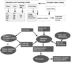Fig. 1

GWSim flow chart. Top: description of the modules of the GWSim code. Available models for the masses: power-Law (PL), power-law with Gaussian (PLG), broken power-law (BPL), multi peak (MP), and the time-delay (TD) model. For the spin: uniform (Uni), heavy-mass (HM), Gaussian spin (GS), and mass-spin correlated (MC). For the merger rate: phenomenological model (PM), time-delay (TD). For the cosmology: ΛCDM w₀CDM, w₀−w_aCDM). Bottom: logical structure of the GWSim code and how the injection samples are produced.

3.2 Simulated GWTC using a galaxy catalog

The primary difference between using or not using a galaxy catalog is the underlying spatial distribution of galaxies that GW sources are going to be assigned to. The galaxies in the simulated galaxy catalog contain spatial clustering, whereas when the galaxies are chosen without a galaxy catalog (fake universe case), they do not feature spatial clustering as they are uniformly distributed in comobile volume. The former can be used to explore the cross-correlation technique whereas for the second one, cross-correlation cannot be used.

In the case when a galaxy catalog is used, the code loads from the catalog the galaxies that are assigned with luminosities in a certain band (chosen by a user). The underlying distribution of the redshifts of galaxies (in this case) is the one from the galaxy catalog, before we apply any merger rate model. The distribution of galaxies in the sky depends on the galaxy catalog. Most of the galaxy catalogs are only covering a small fraction of the sky. In this case, GW events are going to originate from that part only. Full sky galaxy catalogs, like GLADE+ (Dálya et al. 2022), can be used to avoid this limitation. In the future, this module will be developed further to include different formation channels of GW sources and host galaxy properties.

At present, the code cannot take into account the galaxy catalog’s incompleteness. This will be added in the future where GWSim will be able to account for galaxies that host GW events but are not present in the galaxy catalog.

Below, we describe a mock galaxy catalog that is incorporated in the GWSim code. We have used the mock galaxy catalog MICE-Grand Challenge Galaxy and Halo Light-cone Catalog (MICECATv2; Fosalba et al. 2014, 2015; Crocce et al. 2015) developed using an N-body simulation containing about 70 billion dark matter particles in a 3 Gpc h³ comoving volume. The dark matter halos and galaxies generated from this span a sky area of 5000 deg² and up to a redshift of z = 1.4, with no simulation box repetition. The galaxy catalog is made with the following values of the cosmological parameters for a flat-ΛCDM model Ω_m = 0.25; σ₈ = 0.8; n_s = 0.95; Ω_b = 0.044; Ω_Λ =0.75 and h = 0.7¹.

The redshift distribution in MICECATv2 is shown in Fig. 2. The luminosities and magnitudes of the simulated galaxies are provided in the same bands than actual cosmological surveys: DES (Abbott et al. 2021d), Euclid (Scaramella et al. 2022), COSMOS (Scoville et al. 2007), SDSS (Margony 1999), VISTA (Jarvis et al. 2012). We applied an evolutionary correction to the apparent magnitudes as suggested in MICECATv2². $m_{evol} = m_{true} - 0.8 (\arctan (1.5 z) - 0.1489),$ ${m_{{\rm{evol}}}} = {m_{{\rm{true}}}} - 0.8\,\left( {\arctan \,\left( {1.5\,z} \right) - 0.1489} \right),$ (12)

where m_true is the observed magnitude in the catalog, Z is the true redshift and m_evol is the evolved luminosity in redshift. We use m_evol as the observed apparent magnitude, which is used in the luminosity weighting calculation: the user can ask for the probability for a galaxy to host a merger to be proportional to its absolute luminosity. The galaxy catalog also follows the observed luminosity functions, color distributions, and clustering as a function of luminosity and color at low-Z.

From MICECATv2, GW host galaxies are chosen following the GW merger rate model (discussed in the previous section). At each redshift, for a given merger model and observation time, we calculate the number of GW sources N_GW using Eq. (6). Then, we chose N_GW galaxies from the catalog for every redshift and consider these as the hosts of the GW sources. The galaxies chosen as the hosts of the GW sources can also be chosen based on the luminosity of the galaxies at different user-specified bands. We can use a luminosity weighting to choose the GW sources as follows: $w_{i} = 10^{- 0.4 M_{i}},$ ${w_i} = {10^{ - 0.4\,{M_i}}},$ (13)

where M_i is the absolute magnitude for the ith band, for a specific survey. The value of M depends on different wavelength bands in which galaxies are observed and in this code, a user can choose a specific survey and an observation band. To compute the absolute magnitude of the selected galaxy, one can either use the given absolute magnitudes from MICECATv2 or compute them directly from the true correct apparent magnitudes from Eq. (12) for the ith band as $M_{i} = m_{evol, i} - 5 \log_{10} (\frac{d_{L} (z, H_{0})}{Mpc}) - 25,$ ${M_i} = {m_{{\rm{evol,}}i}} - 5\,{\log _{10}}\,\left( {{{{d_{\rm{L}}}\left( {z,{H_0}} \right)} \over {{\rm{Mpc}}}}} \right) - 25,$ (14)

where d_L(z, H₀) is the luminosity distance of the galaxy, as a function of the measured redshift and the Hubble constant, in units of Mpc.

In the following discussion, we explain how MICECATv2 can be used in GWSim to assign galaxies from the catalog to GWTC events. We start by reading the catalog file and by selecting the data columns that we are interested in. We select the sky location in equatorial coordinates (RA and Dec), the true redshift of the galaxies, and the observed magnitude, m_evol, for a specific band.

Since MICECATv2 is a simulated galaxy catalog, no redshift uncertainty is present. However, GWSim can add redshift uncertainties by taking a certain percentage (user given) of the true redshift and using this as the 1σ standard deviation. It can also apply masking to the catalog, where it counts the number of galaxies per pixel over the entire sky, and when this number is smaller than a certain threshold (user given), it treats the pixel as empty. The masking of the catalog over the sky is shown in Fig. 3, as it can be seen, it covers one-eighth of the sky. This masking function will be more useful in future works that adopt real galaxy catalogs, such as GLADE+, thereby introducing a way to measure the angular completeness in each respective catalog.

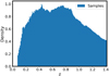Fig. 2

True redshift distribution of galaxies in the simulated catalog MICECATv2.

Fig. 3

Molleview projection of bin count per pixel in MICECATv2.

4 Code validation

The validation of the code is done in two steps. The first one (i) consists in checking that the distributions are correctly sampled. This implies we check whether the mock catalog of GW sources matches the expected population of the GW sources. Then (ii) we produced a mock GW catalog and, by using codes that can infer cosmological parameters from GW data, we try to retrieve the injected cosmological parameters.

Comparison of the GW mock samples with the expected population: Starting from the redshift-independent mass models, various distributions and corresponding samples can be seen in Fig. A.1. The analytical expressions of the distributions are plotted as dashed orange curves whereas the drawn samples are histogrammed in blue. The comoving volume and the merger rate distributions as functions of redshift can be seen in Fig. B.1, as well as samples drawn from them. The code can also assign spins to events sampling from the models described in Table 2. For the results presented from the simulation here, we kept all the spins fixed to zero but an example of sampling of spins for the mass correlated model can be seen in Fig. C.1. Thus, for all relevant parameters such as masses, merger rate, and spin, GWSim can generate mock samples of the desired distribution.

Inference of the injected parameters for O4 Observation run of LIGO-Virgo-KAGRA: GWSim computes the number of expected BBH events for certain values of the merger rate model parameters and an observational time selected by the user. Using a uniform comoving volume distribution as the galaxies’ redshift distribution, we drew hosts of GW events following the merger rate model presented in Eq. (2), with γ = 2.7, κ = 2.9, z_p = 1.9, R₀ = 20 Gpc⁻³ yr⁻¹. We simulated 3 yr of O1−, O2−, O3− and O4−like observation run for a realistic duty cycle with the power law+Gaussian distribution for m₁ that is shown in Fig. A.1 (bottom-left). The duty factors for O1, O2, and O3 were similar to the real ones for the actual LVK observational runs, whereas for O4, we selected values equal to the ones of O3, which can be seen in Table 4.

The total number of mock BBH events is more than 200 thousand (calculated using z_max = 5). Of those, using a network (S/N) threshold (S/N)_thr = 12, only 164 are detected (recalling that the network (S/N) is the (S/N) obtained when combining data from all interferometers). In Fig. 4, we show the kernel density estimate (KDE) of the masses and reshift (all events and detected ones only). This makes the distribution appears smooth. The comparison of the normalized distributions of all the simulated events and detected ones denotes the selection fraction as a function of masses and distance. As heavier sources are more likely to be detected than the lighter ones up to a higher luminosity distance, the distribution of the injected sources and the detected ones differs. This shows the expected distributions of the detected sources with O1+O2+O3+O4 observation with the duty cycle as mentioned in Table 4.

The detected events that pass the (S/N)thr undergo parameter estimation using Bilby, to obtain the posteriors of their parameters, namely individual masses (m₁ and m₂) in detector frame, luminosity distance (D_L), source position (RA and Dec), and the inclination angle (θ_JN) for a single event. Having a set of posterior samples at our disposal allows us to use a population and/or cosmology estimation code and retrieve the injected values. We used the python package IcaroGW which can estimate jointly the population parameters of BBHs and the cosmological parameters (Mastrogiovanni et al. 2021). We used a power-law+Gaussian peak distribution for the primary mass model and the flat-ΛCDM for cosmology. In IcaroGW, we fix Ω_m = 0.3 and allow only H₀ to vary. The posteriors obtained on the black hole population parameters and the Hubble constant for O1+O2+O3+O4 configuration are shown in Fig. 5 along with the injected values (black dashed lines). This joint estimation of 13 parameters including the parameters describing the merger rate parameters (R₀,γ,κ, z_p), black hole mass distribution (α,β, M_max, M_min,µ_g,σ_g,λ_g,δ_m) and cosmology (H₀) presents a forecast for measuring these quantities from the upcoming observation run. The posterior distribution of the population parameters agrees within 95% C.L. with the injected values for most of the parameters. From this joint estimation, the injected value of H₀ is aptly measured from these sources. Among the merger rate-related parameters, we find that the local merger rate R₀ and the power-law index, γ, describing the red-shift evolution of the low redshift merger rate of the binary black holes are well constrained. However, the parameters such as κ and z_p which describe the black hole merger rate at high red-shift are not well constrained, as with the LIGO-Virgo-KAGRA O4 sensitivity, most of the detected binaries lie below redshift z = 1. Among the parameters describing the mass distribution, the parameters such as the power-law index of the masses, α, β, and maximum mass, M_max, are better constrained than the other parameters describing the mass population. This is because these parameters impact a wide range of masses and several detected sources contribute to their estimation. However, some parameters such as M_min,δ_m which captures the minimum mass and smoothing scale of the mass distribution at the lower masses can be poorly constrained as the lower end of the mass distribution is difficult to measure because the sensitivity of detecting lighter sources is smaller. Similarly, at the higher mass end, the parameters such as µ_g, σ_g, and λ_g which capture a localized Gaussian feature in the mass distribution can be constrained by only those sources which are detected around this mass range. With the O4 sensitivity and a duty cycle given in Table 4, only a few sources have been adequately measured, which contributes to constraining these parameters. As a result, due to statistical fluctuations, there is a large scatter in the inference of these parameters. The distribution of the sources in the simulated set agrees well with fiducial values, as shown in Fig. A.1 for the mass distribution mismatch. The mismatch in the estimation of the fiducial value shown in Fig. 5 is due to the statistical fluctuation.

To further explore how the mass distribution gets impacted by the statistical fluctuations, we obtain the distribution of masses m_1,s and m_2,s in the source frame of the detected events with an (S/N) > 12 for different noise realizations (having the same noise power spectrum) with 3 yr and 20 yr of observation time, respectively. In Fig. 6, we show the results for fiducial population, cosmological, population, and detector configuration mentioned in Table 4. The plot shows that with 3 yr of detectable events, different noise realizations cause a larger statistical fluctuation in the probability distribution of masses. However, as the number of sources increases with 20 yr of observation time, the statistical fluctuation reduces, and the mass distribution of the detectable events converges to the expected distribution of the selected events as shown by orange lines in Fig. 4.

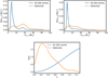Fig. 4

True values of the primary component masses (top left) and lighter component masses (top right) distributions (analytic expression) in the source frame of the detected events for a simulation of O1−, O2−, O3−, and O4−like 3 observational years. The redshifts (bottom) distribution of the events is also shown. The network (S/N) threshold was set to (S/N)_thr = 12. In the same plots, the distribution (KDE estimation) of all the simulated (detected and not detected) events can be seen. The population, cosmological, merger rate, and detector parameters are given in Table 4.

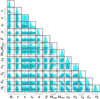Fig. 5

Population and cosmological parameters posteriors obtained from an O1−, O2−, O3−, and O4−like simulation using the cosmological inference python package IcaroGW. The dashed black lines indicate the injected values of parameters.

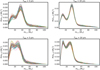Fig. 6

Various m₁ (top) and m₂ (bottom) distributions of the detected events with (S/N) > 12 for T_obs = 3 yr (left) and T_obs = 20 yr (right) produced for different random seeds. Raising the total observational time leads to more events being detected and the distributions being better defined. The population, cosmological, merger rate, and detector parameters used are given in Table 4 and the corresponding distributions are represented by the orange lines of Fig. 4.

5 Conclusions

We present a new GWSim package to simulate GW sources for different cosmological and GW population models. This code can incorporate five scenarios of GW mass models, four scenarios of GW spin distributions, two scenarios of the merger rate, and three models of the cosmological parameters, as described in Fig. 1. The code will be useful to simulate realistic mock samples of the GW sources for different networks of GW detectors. Currently, only second-generation detectors are being used for simulations but in the future, next-generation detectors such as the Cosmic Explorer (Reitze et al. 2019; Hall et al. 2020) and Einstein Telescope (Punturo et al. 2010) will also be included. For a chosen model of the GW source population parameters and cosmological parameters, the code generates samples of binary compact objects for a fixed amount of observation time, duty cycle, and configurations of the detector network. The code can also make use of a simulated galaxy catalog MICECATv2 for assigning the mock GW samples to the redshift and sky position of the host galaxies, possibly using a luminosity weighting. In the future, a revised version will be made to include a real galaxy catalog such as GLADE+ (Dálya et al. 2022) and Duncan (2022). The GWSim code is also wrapped up with the code Bilby for parameter estimation of the GW source parameters. This code will be useful for carrying out simulations of GW sources and understand the interplay between GW source population and cosmology. This code can be used for the currently ongoing network of detectors and also for the next-generation GW detectors.

Acknowledgements

The authors thank Simone Mastrogiovanni for his helpful review of the manuscript as a part of LVK P&P. C. Karathanasis is partially supported by the Spanish MINECO under the grants SEV-2016-0588 and PGC2018-101858-B-I00, some of which include ERDF funds from the European Union. IFAE is partially funded by the CERCA program of the Generalitat de Catalunya. The work of S. Mukherjee is a part of the 〈data | theory〉 Universe-Lab which is supported by the TIFR and the Department of Atomic Energy, Government of India. This analysis is carried out at the computing facility of the LSC cluster. We acknowledge the use of data from the MICE simulations, publicly available at https://cosmohub.pic.es/home. This work has made use of CosmoHub. CosmoHub has been developed by the Port d’Informació Científica (PIC), maintained through a collaboration of the Institut de Física d’Altes Energies (IFAE) and the Centro de Investigaciones Energéticas, Medioambientales y Tecnológicas (CIEMAT) and the Institute of Space Sciences (CSIC and IEEC), and was partially funded by the “Plan Estatal de Investigación Científica y Técnica y de Innovación” program of the Spanish government. We acknowledge the use of the following packages in this work: Astropy (Astropy Collaboration 2013, 2018), Bilby (Ashton et al. 2019), Giant-Triangle-Confusogram (Bocquet & Carter 2016), IPython (Pérez & Granger 2007), Matplotlib (Hunter 2007), NumPy (van der Walt et al. 2011), and SciPy (Jones et al. 2001). The authors are grateful for computational resources provided by the LIGO Laboratory and supported by National Science Foundation Grants PHY-0757058 and PHY-0823459. This research has made use of data or software obtained from the Gravitational Wave Open Science Center (gw-openscience.org), a service of LIGO Laboratory, the LIGO Scientific Collaboration, the Virgo Collaboration, and KAGRA. LIGO Laboratory and Advanced LIGO are funded by the United States National Science Foundation (NSF) as well as the Science and Technology Facilities Council (STFC) of the United Kingdom, the Max-Planck-Society (MPS), and the State of Niedersachsen/Germany for support of the construction of Advanced LIGO and construction and operation of the GEO600 detector. Additional support for Advanced LIGO was provided by the Australian Research Council. Virgo is funded, through the European Gravitational Observatory (EGO), the French Centre National de Recherche Scientifique (CNRS), the Italian Istituto Nazionale di Fisica Nucleare (INFN), and the Dutch Nikhef, with contributions by institutions from Belgium, Germany, Greece, Hungary, Ireland, Japan, Monaco, Poland, Portugal, Spain. The construction and operation of KAGRA are funded by the Ministry of Education, Culture, Sports, Science and Technology (MEXT), Japan Society for the Promotion of Science (JSPS), National Research Foundation (NRF), and Ministry of Science and ICT (MSIT) in Korea, Academia Sinica (AS) and the Ministry of Science and Technology (MoST) in Taiwan. This material is based upon work supported by NSF’s LIGO Laboratory which is a major facility fully funded by the National Science Foundation.

Appendix A Mass distributions

Here, we describe some of the available mass distributions. The implemented mass models are considered for two classes, (i) redshift-independent mass models and (ii) redshift-dependent mass models.

Appendix A.1 Redshift-independent mass models

Appendix A.1.1 Truncated power law

In this case the set of mass distribution parameters is $Λ_{m_{1}} = {M_{m i n}, M_{m a x}, α}$ ${\Lambda _{{m_1}}} = \left\{ {{M_{min}},{M_{max}},\alpha } \right\}$ and the distribution is given by: $p_{P L} (m_{1} | Λ_{m_{1}}) \propto {\begin{array}{l} m_{1}^{- α} & M_{m i n} < m_{1} < M_{m a x} \\ 0 & otherwise \end{array} .$ ${p_{PL}}\left( {\left. {{m_1}} \right|{{\rm{\Lambda }}_{{{\rm{m}}_1}}}} \right) \propto \left\{ {\matrix{ {m_1^{ - \alpha }} \hfill & {{M_{min}} lt; {m_1} lt; {M_{max}}} \hfill \cr 0 \hfill & {{\rm{otherwise}}} \hfill \cr } } \right..$ (A.1)

Appendix A.1.2 Broken power law

In this case, the distribution is a combination of two power-law distributions with indexes a₁,a₂ joined together at a breaking point defined by m_break = M_min + b(M_max − M_min). We also introduced a tapering factor δ_m that smooths the lower end of the distribution. In this case we have $Λ_{m_{1}} = {M_{m i n}, M_{m a x}, α_{1}, α_{2}, b, δ_{m}}$ ${\Lambda _{{m_1}}} = \left\{ {{M_{min}},{M_{max}},{\alpha _1},{\alpha _2},b,{\delta _{\rm{m}}}} \right\}$ and: $\begin{array}{l} p_{B P L} (m_{1} | Λ_{m_{1}}) \propto S (m_{1} | M_{m i n}, δ_{m}) \times \\ {\begin{array}{l} m_{1}^{- α_{1}} & M_{m i n} < m_{1} < m_{b r e a k} \\ m_{1}^{- α_{2}} & m_{b r e a k} < m_{1} < M_{m a x}, \\ 0 & otherwise \end{array} \end{array}$ $\matrix{ {{p_{BPL}}\left( {\left. {{m_1}} \right|{{\rm{\Lambda }}_{{m_1}}}} \right) \propto S\left( {\left. {{m_1}} \right|{M_{min}},{\delta _{\rm{m}}}} \right) \times } \hfill \cr {\,\,\,\,\,\left\{ {\matrix{ {m_1^{ - {\alpha _1}}} \hfill & {{M_{min}} lt; {m_1} lt; {m_{break}}} \hfill \cr {m_1^{ - {\alpha _2}}} \hfill & {{m_{break}} lt; {m_1} lt; {M_{max}},} \hfill \cr 0 \hfill & {{\rm{otherwise}}} \hfill \cr } } \right.} \hfill \cr }$ (A.2)

where: $S (m_{1} | M_{m i n}, δ) = {\begin{array}{l} 0 & m_{1} < M_{m i n} \\ f (m_{1} - M_{m i n}, δ_{m}) & M_{m i n} < m_{1} < M_{m i n} + δ_{m} \\ 1 & m_{1} > M_{m i n} + δ_{m} \end{array},$ $S\left( {\left. {{m_1}} \right|{M_{min}},\delta } \right) = \left\{ {\matrix{ 0 \hfill & {{m_1} lt; {M_{min}}} \hfill \cr {f\left( {{m_1} - {M_{min}},{\delta _{\rm{m}}}} \right)} \hfill & {{M_{min}} lt; {m_1} lt; {M_{min}} + {\delta _{\rm{m}}}} \hfill \cr 1 \hfill & {{m_1} > {M_{min}} + {\delta _{\rm{m}}}} \hfill \cr } } \right.,$ (A.3)

is the smoothing function defined by: $f (m, δ_{m}) = {(1 + \exp (\frac{δ}{m} + \frac{δ}{m - δ}))}^{- 1} .$ $f\left( {m,{\delta _{\rm{m}}}} \right) = {\left( {1 + \exp \left( {{\delta \over m} + {\delta \over {m - \delta }}} \right)} \right)^{ - 1}}.$

Appendix A.1.3 ower law Gaussian

This model is a power-law distribution superimposed with a Gaussian peak distribution with mean µ_g and width σ_g. Here we need an additional parameter that controls the fraction of the Gaussian peak with respect to the power law λ_g. We again used the tapering factor and in this case, we have: $Λ_{m_{1}} = {M_{m i n}, M_{m a x}, α, μ_{g}, σ_{g}, λ_{g}, δ_{m}}$ ${\Lambda _{{m_1}}} = \left\{ {{M_{min}},{M_{max}},\alpha ,{\mu _{\rm{g}}},{\sigma _{\rm{g}}},{\lambda _g},{\delta _{\rm{m}}}} \right\}$ and: $\begin{array}{l} p_{P L G} (m_{1} | Λ_{m_{1}}) \propto S (m_{1} | M_{m i n}, δ_{m}) \times \\ {\begin{array}{l} (1 - λ_{g}) p_{P L} (m_{1} | M_{m a x}, M_{m i n}, α) \\ + λ_{g} G (m_{1} | μ_{g}, σ_{g}) & M_{m i n} < m_{1} < M_{m a x} \\ 0 & otherwise \end{array}, \end{array}$ $\matrix{ {{p_{PLG}}\left( {\left. {{m_1}} \right|{{\rm{\Lambda }}_{{{\rm{m}}_1}}}} \right) \propto S\left( {\left. {{m_1}} \right|{M_{min}},{\delta _{\rm{m}}}} \right) \times } \hfill \cr {\,\,\left\{ {\matrix{ {\left( {1 - {\lambda _{\rm{g}}}} \right){p_{PL}}\left( {\left. {{m_1}} \right|{M_{max}},{M_{min}},\alpha } \right)} \hfill & {} \hfill \cr { + {\lambda _{\rm{g}}}G\left( {\left. {{m_1}} \right|{\mu _{\rm{g}}},{\sigma _{\rm{g}}}} \right)} \hfill & {{M_{min}} lt; {m_1} lt; {M_{max}}} \hfill \cr 0 \hfill & {{\rm{otherwise}}} \hfill \cr } ,} \right.} \hfill \cr }$ (A.4)

where $G (m_{1} | μ_{g}, σ_{g}) = \frac{1}{σ_{g} \sqrt{2 π}} \exp (- \frac{{(m_{1} - μ_{g})}^{2}}{2 σ_{g}^{2}}) .$ $G\left( {\left. {{m_1}} \right|{\mu _{\rm{g}}},{\sigma _{\rm{g}}}} \right) = {1 \over {{\sigma _{\rm{g}}}\sqrt {2\pi } }}\exp \,\left( { - {{{{\left( {{m_1} - {\mu _{\rm{g}}}} \right)}^2}} \over {2\sigma _{\rm{g}}^2}}} \right).$ (A.5)

Appendix A.1.4 Multi-peak

The multi-peak model describes a power-law distribution superimposed with two Gaussian peaks. The distribution is given by: $\begin{array}{l} p_{M P} (m_{1} | Λ_{m_{1}}) \propto S (m_{1} | M_{m i n}, δ_{m}) \times \\ {\begin{array}{l} (1 - λ_{g}) p_{P L} (m_{1} | M_{m a x}, M_{m i n}, α) + \\ λ_{g} (1 - λ_{g, l o w}) G (m_{1} | μ_{g}, σ_{g}) + \\ λ_{g} λ_{g, l o w} G (m_{1} | μ_{g, l o w}, σ_{g, l o w}) & M_{m i n} < m_{1} < M_{m a x} \\ 0 & otherwise \end{array}, \end{array}$ $\matrix{ {{p_{MP}}\left( {\left. {{m_1}} \right|{{\rm{\Lambda }}_{{{\rm{m}}_1}}}} \right) \propto S\left( {\left. {{m_1}} \right|{M_{min}},{\delta _{\rm{m}}}} \right) \times } \hfill \cr {\,\,\left\{ {\matrix{ {\left( {1 - {\lambda _{\rm{g}}}} \right){p_{PL}}\left( {\left. {{m_1}} \right|{M_{max}},{M_{min}},\alpha } \right) + } \hfill & {} \hfill \cr {{\lambda _{\rm{g}}}\left( {1 - {\lambda _{g,low}}} \right)G\left( {\left. {{m_1}} \right|{\mu _{\rm{g}}},{\sigma _{\rm{g}}}} \right) + } \hfill & {} \hfill \cr {{\lambda _{\rm{g}}}{\lambda _{g,low}}G\left( {\left. {{m_1}} \right|{\mu _{g,low}},{\sigma _{g,low}}} \right)} \hfill & {{M_{min}} lt; {m_1} lt; {M_{max}}} \hfill \cr 0 \hfill & {{\rm{otherwise}}} \hfill \cr } } \right.,} \hfill \cr }$ (A.6)

where the parameter λ_g is the fraction of events in the two Gaussian components, while the λ_g,low is the fraction of events in the lower Gaussian component.

Finally, the probability density function of the mass of the lightest black hole (m₂) is defined by: $p (m_{2} | m_{1}) \propto {\begin{array}{l} m_{2}^{β} & M_{m i n} < m_{2} < m_{1} \\ 0 & otherwise \end{array} .$ $p\left( {\left. {{m_2}} \right|{m_1}} \right) \propto \left\{ {\matrix{ {m_2^\beta } \hfill & {{M_{min}} lt; {m_2} lt; {m_1}} \hfill \cr 0 \hfill & {{\rm{otherwise}}} \hfill \cr } } \right..$ (A.7)

It is a conditional power law in the mass interval [M_min; m₁], conditioned on the value of m₁.

Appendix A.2 Redshift-dependent mass models

The phenomenological redshift-dependent mass model allows us to make the simulation of the redshift evolution of the astrophysical population of compact objects and enables us to study of how well such effects can be measured from GW observations. We have considered the phenomenological redshift-dependent model for all the models described in Appendix A.1.1–A.1.4, namely: (i) the truncated power-law, (ii) broken power law, (iii) power-law Gaussian, and (iv) multi-peak model. We allowed for a linear variation in the model parameters with redshift for all these models. We describe below the redshift dependence of the parameters considered in the analysis.

Appendix A.2.1 Redshift-dependent truncated power law model

In this case, we can allow for a variation in the parameters M_min, M_max and α as $\begin{array}{l} M_{m i n} (z) = M_{m i n} + ϵ_{M_{m i n}} z, \\ M_{m a x} (z) = M_{m a x} + ϵ_{M_{m a x}} z, \\ α (z) = α + ϵ_{α} z . \end{array}$ $\matrix{ {{M_{min}}\left( z \right) = {M_{min}} + {_{{M_{min}}}}z,} \hfill \cr {{M_{max}}\left( z \right) = {M_{max}} + {_{{M_{max}}}}z,} \hfill \cr {\,\,\,\,\,\,\,\,\alpha \left( z \right) = \alpha + {_\alpha }z.} \hfill \cr }$ (A.8)

The probability distribution is described by $p_{P L} (m_{1} | Λ_{m_{1}}^{z}) \propto {\begin{array}{l} m_{1}^{- α (z)} & M_{m i n} (z) < m_{1} < M_{m a x} (z) \\ 0 & otherwise \end{array}$ ${p_{PL}}\left( {\left. {{m_1}} \right|{\rm{\Lambda }}_{{{\rm{m}}_1}}^z} \right) \propto \left\{ {\matrix{ {m_1^{ - \alpha \left( z \right)}} \hfill & {{M_{min}}\left( z \right) lt; {m_1} lt; {M_{max}}\left( z \right)} \hfill \cr 0 \hfill & {{\rm{otherwise}}} \hfill \cr } } \right.$ (A.9)

Appendix A.2.2 Redshift-dependent broken power law model

For the redshift-dependent broken power-law model, we allow for a linear evolution of the model parameters with redshift. The evolution of the model parameters can be expressed as: $\begin{array}{l} M_{m i n} (z) = M_{m i n} + ϵ_{M_{m i n}} z, \\ M_{m a x} (z) = M_{m a x} + ϵ_{M_{m a x}} z, \\ α_{1} (z) = α_{1} + ϵ_{α_{1}} z, \\ α_{2} (z) = α_{2} + ϵ_{α_{2}} z, \\ b (z) = b + ϵ_{b} z, \\ δ_{m} (z) = δ_{m} + ϵ_{δ_{m}} z . \end{array}$ $\matrix{ {{M_{min}}\left( z \right) = {M_{min}} + {_{{M_{min}}}}z,} \hfill \cr {{M_{max}}\left( z \right) = {M_{max}} + {_{{M_{max}}}}z,} \hfill \cr {\,\,\,\,\,\,\,{\alpha _1}\left( z \right) = {\alpha _1} + {_{{\alpha _1}}}z,} \hfill \cr {\,\,\,\,\,\,\,{\alpha _2}\left( z \right) = {\alpha _2} + {_{{\alpha _2}}}z,} \hfill \cr {\,\,\,\,\,\,\,\,\,\,b\left( z \right) = b + {_b}z,} \hfill \cr {\,\,\,\,\,\,\,{\delta _m}\left( z \right) = {\delta _m} + {_{{\delta _m}}}z.} \hfill \cr }$ (A.10)

The probability distribution of the broken power-law model is $\begin{array}{l} p_{B P L} (m_{1} | Λ_{m_{1}}^{z}) \propto S (m_{1} | M_{m i n} (z)) \times \\ {\begin{array}{l} m_{1}^{- α_{1} (z)} & M_{m i n} (z) < m_{1} < m_{b r e a k} (z) \\ m_{1}^{- α_{2} (z)} & m_{b r e a k} (z) < m_{1} < m_{m a x} (z), \\ 0 & otherwise \end{array} \end{array}$ $\matrix{ {{p_{BPL}}\left( {{m_1}\left| {{\rm{\Lambda }}_{{m_1}}^z} \right.} \right) \propto S\left( {{m_1}\left| {{M_{min}}\left( z \right)} \right.} \right) \times } \hfill \cr {\,\,\,\left\{ {\matrix{ {m_1^{ - {\alpha _1}\left( z \right)}} \hfill & {{M_{min}}\left( z \right) < {m_1} < {m_{break}}\left( z \right)} \hfill \cr {m_1^{ - {\alpha _2}\left( z \right)}} \hfill & {{m_{break}}\left( z \right) < {m_1} < {m_{max}}\left( z \right),} \hfill \cr 0 \hfill & {\,\,\,{\rm{otherwise}}} \hfill \cr } } \right.} \hfill \cr }$ (A.11)

where m_break(z) = M_min(z) + b(z)(M_max(z) − M_min(z)) The functional form of S(m₁|M_min(z),δ_m(z)) is shown in Eq. (A.3).

Appendix A.2.3 Redshift-dependent power-law Gaussian model

The redshift-dependent power-law Gaussian model considers a linear variation in the model parameters with redshift as: $\begin{array}{l} M_{m i n} (z) = M_{m i n} + ϵ M_{m i n} z, \\ M_{m a x} (z) = M_{m a x} + ϵ M_{m a x} z, \\ α (z) = α + ϵ_{α} z, \\ μ_{g} (z) = m u_{g} + ϵ_{m u_{g}} z, \\ σ (z) = σ + ϵ_{σ} z, \\ λ_{g} (z) = λ_{g} + ϵ_{λ_{g}} z, \\ δ_{m} (z) = δ_{m} + ϵ_{δ_{m}} z . \end{array}$ $\matrix{ {{M_{min}}\left( z \right) = {M_{min}} + {M_{min}}z,} \hfill \cr {{M_{max}}\left( z \right) = {M_{max}} + {M_{max}}z,} \hfill \cr {\,\,\,\,\,\,\,\alpha \left( z \right) = \alpha + {_\alpha }z,} \hfill \cr {\,\,\,\,\,{\mu _g}\left( z \right) = m{u_g} + {_{m{u_g}}}z,} \hfill \cr {\,\,\,\,\,\,\,\sigma \left( z \right) = \sigma + {_\sigma }z,} \hfill \cr {\,\,\,\,\,{\lambda _g}\left( z \right) = {\lambda _g} + {_{{\lambda _g}}}z,} \hfill \cr {\,\,\,\,\,{\delta _m}\left( z \right) = {\delta _m} + {_{{\delta _m}}}z.} \hfill \cr }$ (A.12)

The probability distribution of the mass distribution is $\begin{array}{l} p_{P L G} (m_{1} | Λ_{m_{1}}^{z}) \propto S (m_{1} | M_{m i n} (z), δ_{m} (z)) \times \\ {\begin{array}{l} (1 - λ_{g} (z)) p_{P L} (m_{1} | M_{m a x} (z), M_{m i n} (z), α (z)) \\ + λ_{g} (z) G (m_{1} | μ_{g} (z), σ_{g} (z)) & m_{m i n} (z) < m_{1} < m_{m a x} (z), \\ 0 & otherwise, \end{array} \end{array}$ $\matrix{ {{p_{PLG}}\left( {{m_1}\left| {{\rm{\Lambda }}_{{m_1}}^z} \right.} \right) \propto S\left( {{m_1}\left| {{M_{min}}\left( z \right)},{\delta _m}\left( z \right) \right.} \right) \times } \hfill \cr {\,\,\,\left\{ {\matrix{ {\left( {1 - {\lambda _g}\left( z \right)} \right){p_{PL}}\left( {{m_1}\left| {{M_{max}}\left( z \right),{M_{min}}\left( z \right),\alpha \left( z \right)} \right.} \right)} \hfill & {} \hfill \cr { + {\lambda _g}\left( z \right)G\left( {{m_1}\left| {{\mu _g}\left( z \right),{\sigma _g}\left( z \right)} \right.} \right)} \hfill & {{m_{min}}\left( z \right) < {m_1} < {m_{max}}\left( z \right),} \hfill \cr 0 \hfill & {\,\,\,{\rm{otherwise,}}} \hfill \cr } } \right.} \hfill \cr }$ (A.13)

where the functional form of G(m₁ |μ_g(z), σ_g(z)) is: $G (m_{1} | μ_{g} (z), σ_{g} (z)) = \frac{1}{σ_{g} (z) \sqrt{2 π}} \exp (- \frac{{(m_{1} - μ_{g} (z))}^{2}}{2 σ_{g}^{2} (z)}) .$ $G\left( {{m_1}\left| {{\mu _g}\left( z \right),{\sigma _g}\left( z \right)} \right.} \right) = {1 \over {{\sigma _g}\left( z \right)\sqrt {2\pi } }}\exp \left( { - {{{{\left( {{m_1} - {\mu _g}\left( z \right)} \right)}^2}} \over {2\sigma _g^2\left( z \right)}}} \right).$ (A.14)

Appendix A.2.4 Redshift-dependent multi-peak model

The redshift-dependent multi-peak model allows for the redshift evolution of the peaks in the mass distribution. We consider the redshift evolution of the parameters as: $\begin{array}{l} M_{m i n} (z) = M_{m i n} + ϵ M_{m i n} z, \\ M_{m a x} (z) = M_{m a x} + ϵ M_{m a x} z, \\ α (z) = α + ϵ_{α} z, \\ μ_{g} (z) = m u_{g} + ϵ_{m u_{g}} z, \\ σ (z) = σ + ϵ_{σ} z, \\ λ_{g} (z) = λ_{g} + ϵ_{λ_{g}} z, \\ μ_{g, l o w} (z) = m u_{g, l o w} + ϵ_{m u_{g, l o w}} z, \\ σ_{g, l o w} (z) = σ_{g, l o w} + ϵ_{σ_{g, l o w}} z, \\ λ_{g, l o w} (z) = λ_{g, l o w} + ϵ_{λ_{g, l o w}} z, \\ δ_{m} (z) = δ_{m} + ϵ_{δ_{m}} z, \end{array}$ $\matrix{ {\,\,{M_{min}}\left( z \right) = {M_{min}} + {M_{min}}z,} \hfill \cr {\,\,{M_{max}}\left( z \right) = {M_{max}} + {M_{max}}z,} \hfill \cr {\,\,\,\,\,\,\,\,\,\alpha \left( z \right) = \alpha + {_\alpha }z,} \hfill \cr {\,\,\,\,\,\,{\mu _g}\left( z \right) = m{u_g} + {_{m{u_g}}}z,} \hfill \cr {\,\,\,\,\,\,\,\,\sigma \left( z \right) = \sigma + {_\sigma }z,} \hfill \cr {\,\,\,\,\,\,{\lambda _g}\left( z \right) = {\lambda _g} + {_{{\lambda _g}}}z,} \hfill \cr {{\mu _{g,low}}\left( z \right) = m{u_{g,low}} + {_{m{u_{g,low}}}}z,} \hfill \cr {{\sigma _{g,low}}\left( z \right) = {\sigma _{g,low}} + {_{{\sigma _{g,low}}}}z,} \hfill \cr {{\lambda _{g,low}}\left( z \right) = {\lambda _{g,low}} + {_{{\lambda _{g,low}}}}z,} \hfill \cr {\,\,\,\,\,{\delta _m}\left( z \right) = {\delta _m} + {_{{\delta _m}}}z,} \hfill \cr }$ (A.15)

The probability distribution of the mass distribution is $\begin{array}{l} A p_{M P} (m_{1} | Λ_{m_{1}}^{z}) \propto S (m_{1} | M_{m i n} (z), δ_{m} (z)) \times \\ {\begin{array}{l} (1 - λ_{g} (z)) p_{P L} (m_{1} | M_{m a x} (z), M_{m i n} (z), α (z)) + \\ λ_{g} (z) (1 - λ_{g, l o w} (z)) G (m_{1} | μ_{g} (z), σ_{g} (z)) + \\ λ_{g} (z) λ_{g, l o w} (z) G (m_{1} | μ_{g, l o w} (z), σ_{g, l o w} (z)) & M_{m i n} (z) < m_{1} < M_{m a x} (z) \\ 0 & otherwise \end{array} \end{array}$ $\matrix{ {A{p_{MP}}\left( {{m_1}\left| {{\rm{\Lambda }}_{{{\rm{m}}_1}}^z} \right.} \right) \propto \,S\left( {{m_1}\left|{M_{min}}\left( z \right),{\delta _{\rm{m}}}\left( z \right)} \right) \times } \hfill \cr {\,\,\,\,\left\{ {\matrix{ {\left( {1 - {\lambda _g}\left( z \right)} \right){p_{PL}}\left( {{m_1}\left| {{M_{max}}\left( z \right),{M_{min}}\left( z \right),\alpha \left( z \right)} \right.} \right) + } \hfill & {} \hfill \cr {{\lambda _g}\left( z \right)\left( {1 - {\lambda _{g,low}}\left( z \right)} \right)G\left( {{m_1}\left| {{\mu _g}\left( z \right),{\sigma _g}\left( z \right)} \right.} \right) + } \hfill & {} \hfill \cr {{\lambda _g}\left( z \right){\lambda _{g,low}}\left( z \right)G\left( {{m_1}\left| {{\mu _{g,low}}\left( z \right),{\sigma _{g,low}}\left( z \right)} \right.} \right)} \hfill & {{M_{min}}\left( z \right) & {m_1} < {M_{max}}\left( z \right)} \hfill \cr 0 \hfill & {\,\,\,\,\,\,\,\,\,\,\,\,\,\,\,\,{\rm{otherwise}}} \hfill \cr } } \right.} \hfill \cr }$ (A.16)

where the functional form of G(m₁|μ_g(z),σ_g(z)) given in Eq. (A.14).

Appendix A.2.5 Mixing-mass model

To capture the mass distribution of BBHs at a given merging redshift, z_m, we consider the following: $\begin{array}{r} p_{T D} (m_{1} | z_{m}, Λ_{m_{1}}, Λ_{d}, Λ_{n u i s}) = p (m_{1} | z_{m}, Λ_{m_{1}}) W_{t_{d}} (m_{1}; z_{m}) \\ \times S (m_{1} | M_{m i n}, δ_{m}), \end{array}$ $\matrix{ \hfill {{p_{TD}}\left( {{m_1}\left| {{z_{\rm{m}}},{{\rm{\Lambda }}_{{m_1}}},{{\rm{\Lambda }}_d},} \right.{{\rm{\Lambda }}_{nuis}}} \right) = p\left( {{m_1}\left| {{z_{\rm{m}}},{{\rm{\Lambda }}_{{m_1}}}} \right.} \right){W_{{t_{\rm{d}}}}}\left( {{m_1};{z_{\rm{m}}}} \right)} \cr \hfill { \times S\left( {{m_1}\left| {{M_{min}},{\delta _{\rm{m}}}} \right.} \right),} \cr }$ (A.17)

where the window function W_td(m; z_m) is calculated using: $W_{t_{d}} (m; z_{m}) = N \int_{z_{m}}^{\infty} P_{t} (t_{d} | t_{d}^{m i n}, t_{d}^{m a x}, d) \frac{d t}{d z_{f}} W (m; z_{f}) d z_{f},$ ${W_{{t_{\rm{d}}}}}\left( {m;{z_{\rm{m}}}} \right) = N\int_{{z_{\rm{m}}}}^\infty {{P_t}\left( {\left. {{t_{\rm{d}}}} \right|t_{\rm{d}}^{min},t_{\rm{d}}^{max},d} \right){{{\rm{d}}t} \over {{\rm{d}}{z_{\rm{f}}}}}W\left( {m;{z_{\rm{f}}}} \right){\rm{d}}{z_{\rm{f}}},}$ (A.18)

where N is a normalization factor, P_t is the delay time distribution, W[m(z)] is a Heaviside step function W(m; z_f) = Θ(M_PISN(Z_f) − m), and z_f is the redshift of the formation of a BH. The $W_{t_{d}}$ ${W_{{t_{\rm{d}}}}}$ function brings a breaking point M_break at the mass distribution. The delay time distribution is taken to be a simple power-law function of the delay time t_d: $P_{t} (t_{d} | t_{d}^{m i n}, t_{d}^{m a x}, d) \propto {\begin{array}{l} {(t_{d})}^{- d} & for t_{d}^{m i n} < t_{d} < t_{d}^{m a x}, \\ 0 & otherwise, \end{array}$ ${P_t}\left( {\left. {{t_{\rm{d}}}} \right|t_{\rm{d}}^{min},t_{\rm{d}}^{max},d} \right) \propto \left\{ {\matrix{ {{{\left( {{t_{\rm{d}}}} \right)}^{ - d}}} \hfill & {{\rm{for}}\,t_{\rm{d}}^{min} < {t_{\rm{d}}} < t_{\rm{d}}^{max},} \hfill \cr 0 \hfill & {{\rm{otherwise,}}} \hfill \cr } } \right.$ (A.19)

and the delay time is given by t_d = t_m − t_f, with the notation t_m = t(z_m), t_f = t(z_f) to be the time of merger and time of formation, respectively. The distribution of mi in the source frame p(m₁ | z_m, Φ_m₁) is considered to be given by a power-law distribution superpositioned with the distribution of a Gaussian peak: $\begin{array}{l} p (m_{1} | z_{m} Λ_{m_{1}}) = (1 - λ_{g}) P (m_{1} | M_{m i n}, M_{m a x}, - α) + \\ λ_{g} G (m_{1} | M_{break} (z_{m}), σ_{g}), \end{array}$ $\matrix{ {p\left( {\left. {{m_1}} \right|{z_m}{\Lambda _{{m_1}}}} \right) = \left( {1 - {\lambda _{\rm{g}}}} \right)P\left( {\left. {{m_1}} \right|{M_{min}},{M_{max}}, - \alpha } \right) + } \hfill \cr {\,\,\,\,\,\,\,\,\,\,\,\,\,\,\,\,\,\,\,\,\,\,\,\,\,\,\,\,\,\,\,\,\,\,\,\,\,\,\,\,\,\,\,\,\,\,\,\,\,\,\,\,\,\,\,\,\,\,\,\,\,\,\,\,\,\,\,\,\,\,\,\,\,\,\,\,\,\,\,{\lambda _g}G\left( {\left. {{m_1}} \right|{M_{{\rm{break}}}}\left( {{z_{\rm{m}}}} \right),{\sigma _{\rm{g}}}} \right),} \hfill \cr }$ (A.20)

where $Λ_{m_{1}} = {M_{m i n}, M_{m a x}, α, λ_{g}, M_{break} (z_{m}), σ_{g}}$ ${\Lambda _{{m_1}}} = \left\{ {{M_{min}},{M_{max}},\alpha ,{\lambda _g},{M_{{\rm{break}}}}\left( {{z_{\rm{m}}}} \right),{\sigma _{\rm{g}}}} \right\}$ , G(m₁|M_break(z_m), σg) (as defined in Eq. A.5) and P(m₁ |M_min, M_max, −α) is a power-law distribution with slope −α between M_min and M_max.

In Fig. A.1, the histogram of the samples drawn from the input distributions is shown in blue and the analytical curves are shown as orange dashed curves.

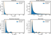Fig. A.1

Empirical distributions (in blue) of the source-frame mass samples drawn from various mass distributions. The analytical expressions of the distributions are plotted in orange dashed curves. Top-left: Truncated power-law model. Top-right: broken-power law model with smoothing at the lower end of the distribution. Bottom-left: a power-law+Gaussian peak model with smoothing at the lower end of the distribution. Bottom-right: a multi-peak model with smoothing at the lower end of the distribution.

Appendix B Merger rate distributions

Here we show some of the available merger rate distributions and showcase the ability of the code to properly sample those distributions.

Appendix B.1 Star formation rate-like BBH merger model

In this case, the distribution is similar to that of Madau & Dickinson (2014), which is characterized by a low-redshift power-law slope, γ, a peak at redshift, z_p, and a high-redshift power-law slope, κ, after the peak: $R (z) = \frac{d N}{d t_{s} d V_{c}} = R_{0} [1 + {(1 + z_{p})}^{- γ - κ}] \frac{{(1 + z)}^{γ}}{1 + {[(1 + z) / (1 + z_{p})]}^{γ + κ}} .$ $R\left( z \right) = {{{\rm{d}}N} \over {{\rm{d}}{t_s}{\rm{d}}{V_{\rm{c}}}}} = {R_0}\left[ {1 + {{\left( {1 + {z_{\rm{p}}}} \right)}^{ - \gamma - \kappa }}} \right]{{{{\left( {1 + z} \right)}^\gamma }} \over {1 + {{\left[ {{{\left( {1 + z} \right)} \mathord{\left/ {\vphantom {{\left( {1 + z} \right)} {\left( {1 + {z_{\rm{p}}}} \right)}}} \right. \kern-\nulldelimiterspace} {\left( {1 + {z_{\rm{p}}}} \right)}}} \right]}^{\gamma + \kappa }}}}.$ (B.1)

Appendix B.2 Time delay BBH merger rate

In the model that takes into account the time delay, the BBH merger rate at a merging redshift z_m is given by: $R_{T D} (z_{m}) = R_{0} \frac{\int_{z_{m}}^{\infty} P_{t} (t_{d} | t_{d}^{m i n}, t_{d}^{m a x}, d) R (z_{f}) \frac{d t}{d z_{f}} d z_{f}}{\int_{0}^{\infty} P_{t} (t_{d} | t_{d}^{m i n}, t_{d}^{m a x}, d) R (z_{f}) \frac{d t}{d z_{f}} d z_{f}},$ ${R_{TD}}\left( {{z_{\rm{m}}}} \right) = {R_0}{{\int_{{z_{\rm{m}}}}^\infty {{P_t}\left( {\left. {{t_{\rm{d}}}} \right|t_{\rm{d}}^{min},t_{\rm{d}}^{max},d} \right)R\left( {{z_{\rm{f}}}} \right){{{\rm{d}}t} \over {{\rm{d}}{z_{\rm{f}}}}}{\rm{d}}{z_{\rm{f}}}} } \over {\int_0^\infty {{P_t}\left( {\left. {{t_{\rm{d}}}} \right|t_{\rm{d}}^{min},t_{\rm{d}}^{max},d} \right)R\left( {{z_{\rm{f}}}} \right){{{\rm{d}}t} \over {{\rm{d}}{z_{\rm{f}}}}}{\rm{d}}{z_{\rm{f}}}} }},$ (B.2)

where R₀ ≡ R(z = 0) is defined as the merger rate at z = 0.

In Fig. B.1, the samples drawn from the distributions are histogrammed in blue and the analytical curves are shown as orange dashed curves.

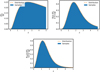Fig. B.1

Empirical distribution of the redshift samples draws (in blue) from the uniform in comoving volume distribution (top left), the merger rate model of Eq. 2 (top right) for z_p = 1.9, γ = 2.7, Κ = 2.9, and the merger rate model in the case of time delay model described by Eq. 4 (bottom) for d = −1, $t_{d}^{m i n} = 0.5$ $t_{\rm{d}}^{min} = 0.5$ Gyrs. The analytical expressions of the distributions are plotted in orange dashed curves. Results obtained using the parameters values given in Table 4.

Appendix C Spin distributions

Various spin distributions are available within the code for both (i) redshift-independent models and (ii) redshift-dependent models. Here, we discuss the available distributions.

Appendix C.1 Redshift-dependent spin model

Appendix C.1.1 Uniform distribution

The simplest implemented spin distribution is the uniform one where: $P (χ_{eff}) \propto 𝒰 [- 1, 1],$ $P\left( {{\chi _{{\rm{eff}}}}} \right) \propto U\left[ { - 1,1} \right],$ (C.1)

and where 𝒰 is the uniform distribution.

Appendix C.1.2 Heavy-mass model

This distribution allows for a correlation of the spins with the masses of the black holes. In this case, individual spins of the black holes are drawn from: $P (χ | m_{th}) \propto {\begin{array}{l} 𝒰 [- 1, 1] & for m > m_{th}, \\ 0 & for m < m_{th} . \end{array}$ $P\left( {\left. \chi \right|{m_{{\rm{th}}}}} \right) \propto \left\{ {\matrix{ {U\left[ { - 1,1} \right]} \hfill & {{\rm{for}}\,m > {m_{{\rm{th}}}},} \hfill \cr 0 \hfill & {{\rm{for}}\,m < {m_{{\rm{th}}}}.} \hfill \cr } } \right.$ (C.2)

This model allows for black holes with masses higher than a selected mass threshold m_th to have non-zero spins.

Appendix C.1.3 Gaussian spins

Here χ_eff is taken from a Gaussian distribution: $P (χ_{eff} | σ_{χ, 0}, μ_{χ, 0}) \propto G (χ_{eff} | σ_{χ_{e f f}}, μ_{χ_{e f f}}),$ $P\left( {\left. {{\chi _{{\rm{eff}}}}} \right|{\sigma _{\chi ,0}},{\mu _{\chi ,0}}} \right) \propto G\left( {\left. {{\chi _{{\rm{eff}}}}} \right|{\sigma _{{\chi _{eff}}}},{\mu _{{\chi _{eff}}}}} \right),$ (C.3)

where G is the Gaussian distribution as $G (χ_{eff} | σ_{χ, 0}, μ_{χ, 0}) = \frac{1}{σ_{χ, 0} \sqrt{2 π}} \exp (- \frac{{(χ_{eff} - μ_{χ, 0})}^{2}}{2 σ_{χ, 0}^{2}}) .$ $G\left( {\left. {{\chi _{{\rm{eff}}}}} \right|{\sigma _{\chi ,0}},{\mu _{\chi ,0}}} \right) = {1 \over {{\sigma _{\chi ,0}}\sqrt {2\pi } }}\exp \left( { - {{{{\left( {{\chi _{{\rm{eff}}}} - {\mu _{\chi ,0}}} \right)}^2}} \over {2\sigma _{\chi ,0}^2}}} \right).$ (C.4)

Appendix C.1.4 Mass correlated model

This model describes a more complicated correlation between masses and spins. In this case, we have: $\begin{array}{l} p (χ_{eff} | q, μ_{χ, 0}, σ_{χ, 0}, α_{s}, β_{s}) \propto \\ \frac{1}{σ_{(σ_{χ, 0}, β_{s}, q)} χ \sqrt{2 π}} \exp [- \frac{{(χ_{eff} - μ_{χ} (μ_{χ, 0}, α_{s}, q))}^{2}}{2 σ_{χ}^{2} (σ_{χ, 0}, β_{s}, q)}], \end{array}$ $\matrix{ {p\left( {\left. {{\chi _{{\rm{eff}}}}} \right|q,{\mu _{\chi ,0}},{\sigma _{\chi ,0}},{\alpha _{\rm{s}}},{\beta _{\rm{s}}}} \right) \propto } \hfill \cr {\,\,\,\,\,\,\,\,\,\,\,\,\,\,\,\,\,\,\,\,\,\,\,\,\,\,\,\,\,\,\,\,\,\,\,\,\,\,\,\,\,\,\,\,{1 \over {{\sigma _{\left( {{\sigma _{\chi ,0}},{\beta _{\rm{s}}},q} \right)}}\chi \sqrt {2\pi } }}\exp \left[ { - {{{{\left( {{\chi _{{\rm{eff}}}} - {\mu _\chi }\left( {{\mu _{\chi ,0}},{\alpha _{\rm{s}}},q} \right)} \right)}^2}} \over {2\sigma _\chi ^2\left( {{\sigma _{\chi ,0}},{\beta _{\rm{s}}},q} \right)}}} \right],} \hfill \cr }$ (C.5)

where μ_χ = µ_χ,0 + α_s(q − 1/2) and 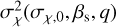$σ_{χ}^{2} (σ_{χ, 0}, β_{s}, q)$ $\sigma _\chi ^2\left( {{\sigma _{\chi ,0}},{\beta _{\rm{s}}},q} \right)$ such that log₁₀ σ_χ(σ_χ,0,β_s,q) = log₁₀ σ_χ,0+ ß_s(q − 1/2). Here we show a spin sampling of the mass correlated model. In Fig. C.1 one can see the samples that the code drew in the χ_eff − q space, χ₁ − q space, and χ₂ − q space. Figure C.2 shows the individual spin amplitudes χ₁ and χ₂ as a function of z in the case of the spin-redshift model where both the expectation value and standard deviation depend linearly of z (see Sect. 2.4.2).

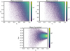Fig. C.1

2D distribution of the spin sampling for the case of the mass correlated model. Top figures: Individual spin amplitudes χ₁ (left) and χ₂ (right) as a function of the mass ratio q. Bottom: Effective spin amplitude, χ_eff, as a function of the mass ratio, q. The distributions are calculated with α_s = 0.013,β_s = −1.53,χ₀ = 0.2, σ₀ = 0.52. The mass distribution is the power-law+Gaussian distribution seen in A.1.

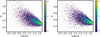Fig. C.2

2D distribution of the sampled spin amplitudes χ₁ (left) and χ₂ (right) for the case of the spin model evolving with the redshift. The parameters used are χ₀ = 0.8, δχ = −0.3, σ₀ = 0.3, δσ = −0.17 (see Sect. 2.4.2 for the spin-redshift dependence).

Appendix C.2 Redshift-dependent spin model

For the redshift-dependent spin model, we considered the redshift-dependent Gaussian model. We allowed for a redshift evolution of the mean value of effective spin μ_χ,0(z) and standard deviation of σ_χ,0(z) as: $\begin{array}{l} μ_{χ, 0} (z) = μ_{χ, 0} + δ χ z, \\ σ_{χ, 0} (z) = σ_{χ, 0} + δ σ z . \end{array}$ $\matrix{ {{\mu _{\chi ,0}}\left( z \right) = {\mu _{\chi ,0}} + \delta \chi z,} \hfill \cr {{\sigma _{\chi ,0}}\left( z \right) = {\sigma _{\chi ,0}} + \delta \sigma z.} \hfill \cr }$ (C.6)

The value of χ_eff is taken from a Gaussian distribution, as follows: $G (χ_{eff} | σ_{χ, 0} (z), μ_{χ, 0} (z)) = \frac{1}{σ_{χ, 0} (z) \sqrt{2 π}} \exp (- \frac{{(χ_{eff} - μ_{χ, 0} (z))}^{2}}{2 σ_{χ, 0} {(z)}^{2}}) .$ $G\left( {\left. {{\chi _{{\rm{eff}}}}} \right|{\sigma _{\chi ,0}}\left( z \right),{\mu _{\chi ,0}}\left( z \right)} \right) = {1 \over {{\sigma _{\chi ,0}}\left( z \right)\sqrt {2\pi } }}\exp \left( { - {{{{\left( {{\chi _{{\rm{eff}}}} - {\mu _{\chi ,0}}\left( z \right)} \right)}^2}} \over {2{\sigma _{\chi ,0}}{{\left( z \right)}^2}}}} \right).$ (C.7)

References

Abbott, B. P., et al. (LIGO Scientific Collaboration & Virgo Collaboration) 2016, Phys. Rev. Lett., 116, 131103 [NASA ADS] [CrossRef] [Google Scholar]
Abbott, B. P., Abbott, R., Abbott, T. D., et al. 2018, Living Rev. Rel., 21, 3 [NASA ADS] [CrossRef] [Google Scholar]
Abbott, B. P., et al. (LIGO Scientific Collaboration & Virgo Collaboration) 2019a, Phys. Rev. X, 9, 031040 [Google Scholar]
Abbott, B. P., Abbott, R., Abbott, T. D., et al. 2019b, ApJ, 882, L24 [Google Scholar]
Abbott, R., Abbott, T. D., Abraham, S., et al. 2020, ApJ, 896, L44 [Google Scholar]
Abbott, B. P., Abbott, R., Abbott, T. D., et al. 2021a, ApJ, 909, 218 [NASA ADS] [CrossRef] [Google Scholar]
Abbott, R., Abbott, T. D., Abraham, S., et al. 2021b, ApJ, 913, L7 [NASA ADS] [CrossRef] [Google Scholar]
Abbott, R., et al. (LIGO Scientific Collaboration & Virgo Collaboration) 2021c, Phys. Rev. X, 11, 021053 [Google Scholar]
Abbott, T. M. C., Adamów, M., Aguena, M., et al. 2021d, ApJS, 255, 20 [NASA ADS] [CrossRef] [Google Scholar]
Abbott, R., et al. (LIGO Scientific Collaboration, Virgo Collaboration, & KAGRA Collaboration) 2023a, Phys. Rev. X, 13, 011048 [NASA ADS] [Google Scholar]
Abbott, R., Abe, H., Acernese, F., et al. 2023b, ApJ, 949, 76 [NASA ADS] [CrossRef] [Google Scholar]
Acernese, F., Agathos, M., Agatsuma, K., et al. 2014, Class. Quant. Grav., 32, 024001 [Google Scholar]
Akutsu, T., Ando, M., Arai, K., et al. 2021, Progr. Theor. Exp. Phys., 2021, 05A101 [CrossRef] [Google Scholar]
Arabsalmani, M., Sahni, V., & Saini, T. D. 2013, Phys. Rev. D, 87, 083001 [NASA ADS] [CrossRef] [Google Scholar]
Ashton, G., Hübner, M., Lasky, P. D., et al. 2019, ApJS, 241, 27 [NASA ADS] [CrossRef] [Google Scholar]
Aso, Y., Michimura, Y., Somiya, K., et al. 2013, Phys. Rev. D, 88, 043007 [NASA ADS] [CrossRef] [Google Scholar]
Astropy Collaboration (Robitaille, T. P., et al.) 2013, A&A, 558, A33 [NASA ADS] [CrossRef] [EDP Sciences] [Google Scholar]
Astropy Collaboration (Price-Whelan, A. M., et al.) 2018, AJ, 156, 123 [Google Scholar]
Banerjee, S., Baumgardt, H., & Kroupa, P. 2010, MNRAS, 402, 371 [Google Scholar]
Bavera, S. S., Fragos, T., Qin, Y., et al. 2020, A&A, 635, A97 [NASA ADS] [CrossRef] [EDP Sciences] [Google Scholar]
Bera, S., Rana, D., More, S., & Bose, S. 2020, ApJ, 902, 79 [NASA ADS] [CrossRef] [Google Scholar]
Biscoveanu, S., Isi, M., Varma, V., & Vitale, S. 2021a, Phys. Rev. D, 104, 103018 [CrossRef] [Google Scholar]
Biscoveanu, S., Isi, M., Vitale, S., & Varma, V. 2021b, Phys. Rev. Lett., 126, 171103 [CrossRef] [Google Scholar]
Biscoveanu, S., Callister, T. A., Haster, C.-J., et al. 2022, ApJ, 932, L19 [NASA ADS] [CrossRef] [Google Scholar]
Bocquet, S., & Carter, F. W. 2016, J. Open Source Softw., 1, 46 [NASA ADS] [CrossRef] [Google Scholar]
Cañas-Herrera, G., Contigiani, O., & Vardanyan, V. 2021, ApJ, 918, 20 [Google Scholar]
Callister, T. A., Haster, C.-J., Ng, K. K. Y., Vitale, S., & Farr, W. M. 2021, ApJ, 922, L5 [NASA ADS] [CrossRef] [Google Scholar]
Calore, F., Cuoco, A., Regimbau, T., Sachdev, S., & Serpico, P. D. 2020, Phys.Rev. Res., 2, 023314 [CrossRef] [Google Scholar]
Cao, L., Lu, Y., & Zhao, Y. 2018, MNRAS, 474, 4997 [NASA ADS] [CrossRef] [Google Scholar]
Chevallier, M., & Polarski, D. 2001, Int. J. Mod. Phys. D, 10, 213 [Google Scholar]
Cigarrán Díaz, C., & Mukherjee, S. 2022, MNRAS, 511, 2782 [CrossRef] [Google Scholar]
Crocce, M., Castander, F. J., Gaztañaga, E., Fosalba, P., & Carretero, J. 2015, MNRAS, 453, 1513 [NASA ADS] [CrossRef] [Google Scholar]
Dálya, G., Díaz, R., Bouchet, F. R., et al. 2022, MNRAS, 514, 1403 [CrossRef] [Google Scholar]
Del Pozzo, W. 2012, Phys. Rev. D, 86, 043011 [NASA ADS] [CrossRef] [Google Scholar]
Dominik, M., Belczynski, K., Fryer, C., et al. 2012, ApJ, 759, 52 [Google Scholar]
Dominik, M., Berti, E., O’Shaughnessy, R., et al. 2015, ApJ, 806, 263 [Google Scholar]
du Buisson, L., Marchant, P., Podsiadlowski, P., et al. 2020, MNRAS, 499, 5941 [Google Scholar]
Duncan, K. J. 2022, MNRAS, 512, 3662 [NASA ADS] [CrossRef] [Google Scholar]
Elbert, O. D., Bullock, J. S., & Kaplinghat, M. 2018, MNRAS, 473, 1186 [NASA ADS] [CrossRef] [Google Scholar]
Eldridge, J. J., Stanway, E. R., & Tang, P. N. 2019, MNRAS, 482, 870 [NASA ADS] [CrossRef] [Google Scholar]
Ezquiaga, J. M., & Holz, D. E. 2022, Phys. Rev. Lett., 129, 061102 [NASA ADS] [CrossRef] [Google Scholar]
Farmer, R., Renzo, M., de Mink, S. E., Marchant, P., & Justham, S. 2019, ApJ, 887, 53 [Google Scholar]
Farr, W. M., Stevenson, S., Coleman Miller, M., et al. 2017, Nature, 548, 426 [NASA ADS] [CrossRef] [Google Scholar]
Farr, W. M., Fishbach, M., Ye, J., & Holz, D. 2019, ApJ, 883, L42 [NASA ADS] [CrossRef] [Google Scholar]
Finke, A., Foffa, S., Iacovelli, F., Maggiore, M., & Mancarella, M. 2021, J. Cosmol. Astropart. Phys., 2021, 026 [CrossRef] [Google Scholar]
Fishbach, M., & Kalogera, V. 2021, ApJ, 914, L30 [CrossRef] [Google Scholar]
Fishbach, M., Gray, R., Magaña Hernandez, I., et al. 2019, ApJ, 871, L13 [NASA ADS] [CrossRef] [Google Scholar]
Fosalba, P., Gaztañaga, E., Castander, F. J., & Crocce, M. 2014, MNRAS, 447, 1319 [Google Scholar]
Fosalba, P., Crocce, M., Gaztañaga, E., & Castander, F. J. 2015, MNRAS, 448, 2987 [NASA ADS] [CrossRef] [Google Scholar]
Fuller, J., & Ma, L. 2019, ApJ, 881, L1 [Google Scholar]
Gerosa, D., Berti, E., O’Shaughnessy, R., et al. 2018, Phys. Rev. D, 98, 084036 [Google Scholar]
Gray, R., Hernandez, I. M. N., Qi, H., et al. 2020, Phys. Rev. D, 101, 122001 [NASA ADS] [CrossRef] [Google Scholar]
Gregory, M. H. e. a. 2010, Class. Quant. Grav., 27, 084006 [NASA ADS] [CrossRef] [Google Scholar]
Hall, A., Gow, A. D., & Byrnes, C. T. 2020, Phys. Rev. D, 102, 123524 [NASA ADS] [CrossRef] [Google Scholar]
Hunter, J. D. 2007, Comput. Sci. Eng., 9, 90 [NASA ADS] [CrossRef] [Google Scholar]
Jarvis, M. J., Bonfield, D. G., Bruce, V. A., et al. 2012, MNRAS, 428, 1281 [Google Scholar]
Jones, E., Oliphant, T., Peterson, P., et al. 2001, SciPy: Open source scientifictools for Python, http://www.scipy.org/ [Google Scholar]
Karathanasis, C., Mukherjee, S., & Mastrogiovanni, S. 2023, MNRAS, 523, 4539 [NASA ADS] [Google Scholar]
Kushnir, D., Zaldarriaga, M., Kollmeier, J. A., & Waldman, R. 2016, MNRAS, 462, 844 [NASA ADS] [CrossRef] [Google Scholar]
Lamberts, A., Garrison-Kimmel, S., Clausen, D. R., & Hopkins, P. F. 2016, MNRAS, 463, L31 [NASA ADS] [CrossRef] [Google Scholar]
Leyde, K., Mastrogiovanni, S., Steer, D. A., Chassande-Mottin, E., & Karathanasis, C. 2022, JCAP, 09, 012 [CrossRef] [Google Scholar]
Linder, E. V. 2003, Phys. Rev. Lett., 90, 091301 [Google Scholar]
MacLeod, C. L., & Hogan, C. J. 2008, Phys. Rev. D, 77, 043512 [CrossRef] [Google Scholar]
Madau, P., & Dickinson, M. 2014, ARA&A, 52, 415 [Google Scholar]
Mancarella, M., Genoud-Prachex, E., & Maggiore, M. 2022, Phys. Rev. D, 105, 064030 [NASA ADS] [CrossRef] [Google Scholar]
Mandel, I., & de Mink, S. E. 2016, MNRAS, 458, 2634 [NASA ADS] [CrossRef] [Google Scholar]
Mandel, I., & O’Shaughnessy, R. 2010, Class. Quant. Grav., 27, 114007 [NASA ADS] [CrossRef] [Google Scholar]
Margony, B. 1999, Philos. Trans. Roy. Soc. Lond. A: Math. Phys. Eng. Sci., 357, 93 [NASA ADS] [CrossRef] [Google Scholar]
Martynov, D. V., Hall, E. D., Abbott, B. P., et al. 2016, Phys. Rev. D, 93, 112004; Erratum: 2018, 97, 059901 [Google Scholar]
Mastrogiovanni, S., Leyde, K., Karathanasis, C., et al. 2021, Phys. Rev. D, 104, 062009 [NASA ADS] [CrossRef] [Google Scholar]
Mukherjee, S. 2022, MNRAS, 515, 5495 [NASA ADS] [CrossRef] [Google Scholar]
Mukherjee, S., & Dizgah, A. M. 2022, ApJ, 937, L27 [NASA ADS] [CrossRef] [Google Scholar]
Mukherjee, S., & Silk, J. 2021, MNRAS, 506, 3977 [NASA ADS] [CrossRef] [Google Scholar]
Mukherjee, S., & Wandelt, B. D. 2018, ArXiv e-prints [arXiv: 1808.06615] [Google Scholar]
Mukherjee, S., Wandelt, B. D., & Silk, J. 2020, MNRAS, 494, 1956 [Google Scholar]
Mukherjee, S., Wandelt, B. D., Nissanke, S. M., & Silvestri, A. 2021a, Phys. Rev.D, 103, 043520 [NASA ADS] [CrossRef] [Google Scholar]
Mukherjee, S., Wandelt, B. D., & Silk, J. 2021b, MNRAS, 502, 1136 [NASA ADS] [CrossRef] [Google Scholar]
Mukherjee, S., Krolewski, A., Wandelt, B. D., & Silk, J. 2022, ArXiv e-prints [arXiv:2203.03643] [Google Scholar]
Oguri, M. 2016, Phys. Rev. D, 93, 083511 [Google Scholar]
O’Shaughnessy, R., Kalogera, V., & Belczynski, K. 2010, ApJ, 716, 615 [CrossRef] [Google Scholar]
O’Shaughnessy, R., Gerosa, D., & Wysocki, D. 2017, Phys. Rev. Lett., 119, 011101 [CrossRef] [Google Scholar]
Palmese, A., Bom, C. R., Mucesh, S., & Hartley, W. G. 2023, ApJ, 943, 56 [NASA ADS] [CrossRef] [Google Scholar]
Pérez, F., & Granger, B. E. 2007, Comput. Sci. Eng., 9, 21 [Google Scholar]
Punturo, M., Abernathy, M., Acernese, F., et al. 2010, Class. Quant. Grav., 27, 194002 [Google Scholar]
Reitze, D., Adhikari, R. X., Ballmer, S., et al. 2019, Bull. Am. Astron. Soc., 51, 035 [Google Scholar]
Renzo, M., Farmer, R. J., Justham, S., et al. 2020, MNRAS, 493, 4333 [NASA ADS] [CrossRef] [Google Scholar]
Rodriguez, C. L., Zevin, M., Pankow, C., Kalogera, V., & Rasio, F. A. 2016, ApJ, 832, L2 [NASA ADS] [CrossRef] [Google Scholar]
Santoliquido, F., Mapelli, M., Giacobbo, N., Bouffanais, Y., & Artale, M. C. 2021, MNRAS, 502, 4877 [NASA ADS] [CrossRef] [Google Scholar]
Scaramella, R., Amiaux, J., Mellier, Y., et al. 2022, A&A, 662, A112 [NASA ADS] [CrossRef] [EDP Sciences] [Google Scholar]
Scelfo, G., Boco, L., Lapi, A., & Viel, M. 2020, JCAP, 10, 045 [CrossRef] [Google Scholar]
Scelfo, G., Spinelli, M., Raccanelli, A., et al. 2022, JCAP, 01, 004 [CrossRef] [Google Scholar]
Schutz, B. F. 1986, Nature, 323, 310 [Google Scholar]
Scoville, N., Aussel, H., Brusa, M., et al. 2007, ApJS, 172, 1 [Google Scholar]
Soares-Santos, M., Palmese, A., Hartley, W., et al. 2019, ApJ, 876, L7 [NASA ADS] [CrossRef] [Google Scholar]
Spera, M., & Mapelli, M. 2017, MNRAS, 470, 4739 [Google Scholar]
Stevenson, S., Berry, C. P. L., & Mandel, I. 2017, MNRAS, 471, 2801 [NASA ADS] [CrossRef] [Google Scholar]
Talbot, C., & Thrane, E. 2018, ApJ, 856, 173 [NASA ADS] [CrossRef] [Google Scholar]
Tallada, P., Carretero, J., Casals, J., et al. 2020, Astron. Comput., 32, 100391 [Google Scholar]
Taylor, S. R., Gair, J. R., & Mandel, I. 2012, Phys. Rev. D, 85, 023535 [Google Scholar]
The LIGO Scientific Collaboration (Aasi, J., et al.) 2015, Class. Quant. Grav., 32, 074001 [Google Scholar]
The LIGO Scientific Collaboration, the Virgo Collaboration, & the KAGRA Collaboration 2021, ArXiv e-prints [arXiv:2111.03606] [Google Scholar]
The LIGO Scientific Collaboration & the Virgo Collaboration 2021, ArXiv e-prints [arXiv: 2108.01045] [Google Scholar]
Tse, M., Yu, H., Kijbunchoo, N., et al. 2019, Phys. Rev. Lett., 123, 231107 [NASA ADS] [CrossRef] [Google Scholar]
van der Walt, S., Colbert, S. C., & Varoquaux, G. 2011, Comput. Sci. Eng., 13, 22 [Google Scholar]
Vitale, S., Farr, W. M., Ng, K., & Rodriguez, C. L. 2019, ApJ, 886, L1 [NASA ADS] [CrossRef] [Google Scholar]
You, Z.-Q., Zhu, X.-J., Ashton, G., Thrane, E., & Zhu, Z.-H. 2021, ApJ, 908, 215 [NASA ADS] [CrossRef] [Google Scholar]

¹

The catalog is available for download from the CosmoHub website. (Tallada et al. 2020).

²

MICECATv2’s “readme” document (https://www.dropbox.com/s/0ffa8e7463n8h1q/README_MICECAT_v2.0_for_new_CosmoHub.pdf?dl=0).

All Tables

Table 1

Description of the cosmological models available and the parameters that govern them.

In the text

Table 2

Description of the population models available.

In the text

Table 3

Description of the parameters that govern the population models.

In the text

Table 4

Fiducial value of the parameters and duty cycle used in the analysis.

In the text

All Figures

Fig. 1

GWSim flow chart. Top: description of the modules of the GWSim code. Available models for the masses: power-Law (PL), power-law with Gaussian (PLG), broken power-law (BPL), multi peak (MP), and the time-delay (TD) model. For the spin: uniform (Uni), heavy-mass (HM), Gaussian spin (GS), and mass-spin correlated (MC). For the merger rate: phenomenological model (PM), time-delay (TD). For the cosmology: ΛCDM w₀CDM, w₀−w_aCDM). Bottom: logical structure of the GWSim code and how the injection samples are produced.

In the text

	Fig. 2 True redshift distribution of galaxies in the simulated catalog `MICECATv2`.
In the text

	Fig. 3 Molleview projection of bin count per pixel in `MICECATv2`.
In the text

Fig. 4

True values of the primary component masses (top left) and lighter component masses (top right) distributions (analytic expression) in the source frame of the detected events for a simulation of O1−, O2−, O3−, and O4−like 3 observational years. The redshifts (bottom) distribution of the events is also shown. The network (S/N) threshold was set to (S/N)_thr = 12. In the same plots, the distribution (KDE estimation) of all the simulated (detected and not detected) events can be seen. The population, cosmological, merger rate, and detector parameters are given in Table 4.

In the text

	Fig. 5 Population and cosmological parameters posteriors obtained from an O1−, O2−, O3−, and O4−like simulation using the cosmological inference python package `IcaroGW`. The dashed black lines indicate the injected values of parameters.
In the text

Fig. 6

Various m₁ (top) and m₂ (bottom) distributions of the detected events with (S/N) > 12 for T_obs = 3 yr (left) and T_obs = 20 yr (right) produced for different random seeds. Raising the total observational time leads to more events being detected and the distributions being better defined. The population, cosmological, merger rate, and detector parameters used are given in Table 4 and the corresponding distributions are represented by the orange lines of Fig. 4.

In the text

Fig. A.1

Empirical distributions (in blue) of the source-frame mass samples drawn from various mass distributions. The analytical expressions of the distributions are plotted in orange dashed curves. Top-left: Truncated power-law model. Top-right: broken-power law model with smoothing at the lower end of the distribution. Bottom-left: a power-law+Gaussian peak model with smoothing at the lower end of the distribution. Bottom-right: a multi-peak model with smoothing at the lower end of the distribution.

In the text

Fig. B.1

Empirical distribution of the redshift samples draws (in blue) from the uniform in comoving volume distribution (top left), the merger rate model of Eq. 2 (top right) for z_p = 1.9, γ = 2.7, Κ = 2.9, and the merger rate model in the case of time delay model described by Eq. 4 (bottom) for d = −1, $t_{d}^{m i n} = 0.5$ $t_{\rm{d}}^{min} = 0.5$ Gyrs. The analytical expressions of the distributions are plotted in orange dashed curves. Results obtained using the parameters values given in Table 4.

In the text

Fig. C.1

2D distribution of the spin sampling for the case of the mass correlated model. Top figures: Individual spin amplitudes χ₁ (left) and χ₂ (right) as a function of the mass ratio q. Bottom: Effective spin amplitude, χ_eff, as a function of the mass ratio, q. The distributions are calculated with α_s = 0.013,β_s = −1.53,χ₀ = 0.2, σ₀ = 0.52. The mass distribution is the power-law+Gaussian distribution seen in A.1.

In the text

	Fig. C.2 2D distribution of the sampled spin amplitudes χ₁ (left) and χ₂ (right) for the case of the spin model evolving with the redshift. The parameters used are χ₀ = 0.8, δχ = −0.3, σ₀ = 0.3, δσ = −0.17 (see Sect. 2.4.2 for the spin-redshift dependence).
In the text

Current usage metrics show cumulative count of Article Views (full-text article views including HTML views, PDF and ePub downloads, according to the available data) and Abstracts Views on Vision4Press platform.

Data correspond to usage on the plateform after 2015. The current usage metrics is available 48-96 hours after online publication and is updated daily on week days.

Initial download of the metrics may take a while.

[1] Abbott, B. P., et al. (LIGO Scientific Collaboration & Virgo Collaboration) 2016, Phys. Rev. Lett., 116, 131103 [NASA ADS] [CrossRef] [Google Scholar]

[2] Abbott, B. P., Abbott, R., Abbott, T. D., et al. 2018, Living Rev. Rel., 21, 3 [NASA ADS] [CrossRef] [Google Scholar]

[3] Abbott, B. P., et al. (LIGO Scientific Collaboration & Virgo Collaboration) 2019a, Phys. Rev. X, 9, 031040 [Google Scholar]

[4] Abbott, B. P., Abbott, R., Abbott, T. D., et al. 2019b, ApJ, 882, L24 [Google Scholar]

[5] Abbott, R., Abbott, T. D., Abraham, S., et al. 2020, ApJ, 896, L44 [Google Scholar]

[6] Abbott, B. P., Abbott, R., Abbott, T. D., et al. 2021a, ApJ, 909, 218 [NASA ADS] [CrossRef] [Google Scholar]

[7] Abbott, R., Abbott, T. D., Abraham, S., et al. 2021b, ApJ, 913, L7 [NASA ADS] [CrossRef] [Google Scholar]

[8] Abbott, R., et al. (LIGO Scientific Collaboration & Virgo Collaboration) 2021c, Phys. Rev. X, 11, 021053 [Google Scholar]

[9] Abbott, T. M. C., Adamów, M., Aguena, M., et al. 2021d, ApJS, 255, 20 [NASA ADS] [CrossRef] [Google Scholar]

[10] Abbott, R., et al. (LIGO Scientific Collaboration, Virgo Collaboration, & KAGRA Collaboration) 2023a, Phys. Rev. X, 13, 011048 [NASA ADS] [Google Scholar]

[11] Abbott, R., Abe, H., Acernese, F., et al. 2023b, ApJ, 949, 76 [NASA ADS] [CrossRef] [Google Scholar]

[12] Acernese, F., Agathos, M., Agatsuma, K., et al. 2014, Class. Quant. Grav., 32, 024001 [Google Scholar]

[13] Akutsu, T., Ando, M., Arai, K., et al. 2021, Progr. Theor. Exp. Phys., 2021, 05A101 [CrossRef] [Google Scholar]

[14] Arabsalmani, M., Sahni, V., & Saini, T. D. 2013, Phys. Rev. D, 87, 083001 [NASA ADS] [CrossRef] [Google Scholar]

[15] Ashton, G., Hübner, M., Lasky, P. D., et al. 2019, ApJS, 241, 27 [NASA ADS] [CrossRef] [Google Scholar]

[16] Aso, Y., Michimura, Y., Somiya, K., et al. 2013, Phys. Rev. D, 88, 043007 [NASA ADS] [CrossRef] [Google Scholar]

[17] Astropy Collaboration (Robitaille, T. P., et al.) 2013, A&A, 558, A33 [NASA ADS] [CrossRef] [EDP Sciences] [Google Scholar]

[18] Astropy Collaboration (Price-Whelan, A. M., et al.) 2018, AJ, 156, 123 [Google Scholar]

[19] Banerjee, S., Baumgardt, H., & Kroupa, P. 2010, MNRAS, 402, 371 [Google Scholar]

[20] Bavera, S. S., Fragos, T., Qin, Y., et al. 2020, A&A, 635, A97 [NASA ADS] [CrossRef] [EDP Sciences] [Google Scholar]

[21] Bera, S., Rana, D., More, S., & Bose, S. 2020, ApJ, 902, 79 [NASA ADS] [CrossRef] [Google Scholar]

[22] Biscoveanu, S., Isi, M., Varma, V., & Vitale, S. 2021a, Phys. Rev. D, 104, 103018 [CrossRef] [Google Scholar]

[23] Biscoveanu, S., Isi, M., Vitale, S., & Varma, V. 2021b, Phys. Rev. Lett., 126, 171103 [CrossRef] [Google Scholar]

[24] Biscoveanu, S., Callister, T. A., Haster, C.-J., et al. 2022, ApJ, 932, L19 [NASA ADS] [CrossRef] [Google Scholar]

[25] Bocquet, S., & Carter, F. W. 2016, J. Open Source Softw., 1, 46 [NASA ADS] [CrossRef] [Google Scholar]

[26] Cañas-Herrera, G., Contigiani, O., & Vardanyan, V. 2021, ApJ, 918, 20 [Google Scholar]

[27] Callister, T. A., Haster, C.-J., Ng, K. K. Y., Vitale, S., & Farr, W. M. 2021, ApJ, 922, L5 [NASA ADS] [CrossRef] [Google Scholar]

[28] Calore, F., Cuoco, A., Regimbau, T., Sachdev, S., & Serpico, P. D. 2020, Phys.Rev. Res., 2, 023314 [CrossRef] [Google Scholar]

[29] Cao, L., Lu, Y., & Zhao, Y. 2018, MNRAS, 474, 4997 [NASA ADS] [CrossRef] [Google Scholar]

[30] Chevallier, M., & Polarski, D. 2001, Int. J. Mod. Phys. D, 10, 213 [Google Scholar]

[31] Cigarrán Díaz, C., & Mukherjee, S. 2022, MNRAS, 511, 2782 [CrossRef] [Google Scholar]

[32] Crocce, M., Castander, F. J., Gaztañaga, E., Fosalba, P., & Carretero, J. 2015, MNRAS, 453, 1513 [NASA ADS] [CrossRef] [Google Scholar]

[33] Dálya, G., Díaz, R., Bouchet, F. R., et al. 2022, MNRAS, 514, 1403 [CrossRef] [Google Scholar]

[34] Del Pozzo, W. 2012, Phys. Rev. D, 86, 043011 [NASA ADS] [CrossRef] [Google Scholar]

[35] Dominik, M., Belczynski, K., Fryer, C., et al. 2012, ApJ, 759, 52 [Google Scholar]

[36] Dominik, M., Berti, E., O’Shaughnessy, R., et al. 2015, ApJ, 806, 263 [Google Scholar]

[37] du Buisson, L., Marchant, P., Podsiadlowski, P., et al. 2020, MNRAS, 499, 5941 [Google Scholar]

[38] Duncan, K. J. 2022, MNRAS, 512, 3662 [NASA ADS] [CrossRef] [Google Scholar]

[39] Elbert, O. D., Bullock, J. S., & Kaplinghat, M. 2018, MNRAS, 473, 1186 [NASA ADS] [CrossRef] [Google Scholar]

[40] Eldridge, J. J., Stanway, E. R., & Tang, P. N. 2019, MNRAS, 482, 870 [NASA ADS] [CrossRef] [Google Scholar]

[41] Ezquiaga, J. M., & Holz, D. E. 2022, Phys. Rev. Lett., 129, 061102 [NASA ADS] [CrossRef] [Google Scholar]

[42] Farmer, R., Renzo, M., de Mink, S. E., Marchant, P., & Justham, S. 2019, ApJ, 887, 53 [Google Scholar]

[43] Farr, W. M., Stevenson, S., Coleman Miller, M., et al. 2017, Nature, 548, 426 [NASA ADS] [CrossRef] [Google Scholar]

[44] Farr, W. M., Fishbach, M., Ye, J., & Holz, D. 2019, ApJ, 883, L42 [NASA ADS] [CrossRef] [Google Scholar]

[45] Finke, A., Foffa, S., Iacovelli, F., Maggiore, M., & Mancarella, M. 2021, J. Cosmol. Astropart. Phys., 2021, 026 [CrossRef] [Google Scholar]

[46] Fishbach, M., & Kalogera, V. 2021, ApJ, 914, L30 [CrossRef] [Google Scholar]

[47] Fishbach, M., Gray, R., Magaña Hernandez, I., et al. 2019, ApJ, 871, L13 [NASA ADS] [CrossRef] [Google Scholar]

[48] Fosalba, P., Gaztañaga, E., Castander, F. J., & Crocce, M. 2014, MNRAS, 447, 1319 [Google Scholar]

[49] Fosalba, P., Crocce, M., Gaztañaga, E., & Castander, F. J. 2015, MNRAS, 448, 2987 [NASA ADS] [CrossRef] [Google Scholar]

[50] Fuller, J., & Ma, L. 2019, ApJ, 881, L1 [Google Scholar]

[51] Gerosa, D., Berti, E., O’Shaughnessy, R., et al. 2018, Phys. Rev. D, 98, 084036 [Google Scholar]

[52] Gray, R., Hernandez, I. M. N., Qi, H., et al. 2020, Phys. Rev. D, 101, 122001 [NASA ADS] [CrossRef] [Google Scholar]

[53] Gregory, M. H. e. a. 2010, Class. Quant. Grav., 27, 084006 [NASA ADS] [CrossRef] [Google Scholar]

[54] Hall, A., Gow, A. D., & Byrnes, C. T. 2020, Phys. Rev. D, 102, 123524 [NASA ADS] [CrossRef] [Google Scholar]

[55] Hunter, J. D. 2007, Comput. Sci. Eng., 9, 90 [NASA ADS] [CrossRef] [Google Scholar]

[56] Jarvis, M. J., Bonfield, D. G., Bruce, V. A., et al. 2012, MNRAS, 428, 1281 [Google Scholar]

[57] Jones, E., Oliphant, T., Peterson, P., et al. 2001, SciPy: Open source scientifictools for Python, http://www.scipy.org/ [Google Scholar]

[58] Karathanasis, C., Mukherjee, S., & Mastrogiovanni, S. 2023, MNRAS, 523, 4539 [NASA ADS] [Google Scholar]

[59] Kushnir, D., Zaldarriaga, M., Kollmeier, J. A., & Waldman, R. 2016, MNRAS, 462, 844 [NASA ADS] [CrossRef] [Google Scholar]

[60] Lamberts, A., Garrison-Kimmel, S., Clausen, D. R., & Hopkins, P. F. 2016, MNRAS, 463, L31 [NASA ADS] [CrossRef] [Google Scholar]

[61] Leyde, K., Mastrogiovanni, S., Steer, D. A., Chassande-Mottin, E., & Karathanasis, C. 2022, JCAP, 09, 012 [CrossRef] [Google Scholar]

[62] Linder, E. V. 2003, Phys. Rev. Lett., 90, 091301 [Google Scholar]

[63] MacLeod, C. L., & Hogan, C. J. 2008, Phys. Rev. D, 77, 043512 [CrossRef] [Google Scholar]

[64] Madau, P., & Dickinson, M. 2014, ARA&A, 52, 415 [Google Scholar]

[65] Mancarella, M., Genoud-Prachex, E., & Maggiore, M. 2022, Phys. Rev. D, 105, 064030 [NASA ADS] [CrossRef] [Google Scholar]

[66] Mandel, I., & de Mink, S. E. 2016, MNRAS, 458, 2634 [NASA ADS] [CrossRef] [Google Scholar]

[67] Mandel, I., & O’Shaughnessy, R. 2010, Class. Quant. Grav., 27, 114007 [NASA ADS] [CrossRef] [Google Scholar]

[68] Margony, B. 1999, Philos. Trans. Roy. Soc. Lond. A: Math. Phys. Eng. Sci., 357, 93 [NASA ADS] [CrossRef] [Google Scholar]

[69] Martynov, D. V., Hall, E. D., Abbott, B. P., et al. 2016, Phys. Rev. D, 93, 112004; Erratum: 2018, 97, 059901 [Google Scholar]

[70] Mastrogiovanni, S., Leyde, K., Karathanasis, C., et al. 2021, Phys. Rev. D, 104, 062009 [NASA ADS] [CrossRef] [Google Scholar]

[71] Mukherjee, S. 2022, MNRAS, 515, 5495 [NASA ADS] [CrossRef] [Google Scholar]

[72] Mukherjee, S., & Dizgah, A. M. 2022, ApJ, 937, L27 [NASA ADS] [CrossRef] [Google Scholar]

[73] Mukherjee, S., & Silk, J. 2021, MNRAS, 506, 3977 [NASA ADS] [CrossRef] [Google Scholar]

[74] Mukherjee, S., & Wandelt, B. D. 2018, ArXiv e-prints [arXiv: 1808.06615] [Google Scholar]

[75] Mukherjee, S., Wandelt, B. D., & Silk, J. 2020, MNRAS, 494, 1956 [Google Scholar]

[76] Mukherjee, S., Wandelt, B. D., Nissanke, S. M., & Silvestri, A. 2021a, Phys. Rev.D, 103, 043520 [NASA ADS] [CrossRef] [Google Scholar]

[77] Mukherjee, S., Wandelt, B. D., & Silk, J. 2021b, MNRAS, 502, 1136 [NASA ADS] [CrossRef] [Google Scholar]

[78] Mukherjee, S., Krolewski, A., Wandelt, B. D., & Silk, J. 2022, ArXiv e-prints [arXiv:2203.03643] [Google Scholar]

[79] Oguri, M. 2016, Phys. Rev. D, 93, 083511 [Google Scholar]

[80] O’Shaughnessy, R., Kalogera, V., & Belczynski, K. 2010, ApJ, 716, 615 [CrossRef] [Google Scholar]

[81] O’Shaughnessy, R., Gerosa, D., & Wysocki, D. 2017, Phys. Rev. Lett., 119, 011101 [CrossRef] [Google Scholar]

[82] Palmese, A., Bom, C. R., Mucesh, S., & Hartley, W. G. 2023, ApJ, 943, 56 [NASA ADS] [CrossRef] [Google Scholar]

[83] Pérez, F., & Granger, B. E. 2007, Comput. Sci. Eng., 9, 21 [Google Scholar]

[84] Punturo, M., Abernathy, M., Acernese, F., et al. 2010, Class. Quant. Grav., 27, 194002 [Google Scholar]

[85] Reitze, D., Adhikari, R. X., Ballmer, S., et al. 2019, Bull. Am. Astron. Soc., 51, 035 [Google Scholar]

[86] Renzo, M., Farmer, R. J., Justham, S., et al. 2020, MNRAS, 493, 4333 [NASA ADS] [CrossRef] [Google Scholar]

[87] Rodriguez, C. L., Zevin, M., Pankow, C., Kalogera, V., & Rasio, F. A. 2016, ApJ, 832, L2 [NASA ADS] [CrossRef] [Google Scholar]

[88] Santoliquido, F., Mapelli, M., Giacobbo, N., Bouffanais, Y., & Artale, M. C. 2021, MNRAS, 502, 4877 [NASA ADS] [CrossRef] [Google Scholar]

[89] Scaramella, R., Amiaux, J., Mellier, Y., et al. 2022, A&A, 662, A112 [NASA ADS] [CrossRef] [EDP Sciences] [Google Scholar]

[90] Scelfo, G., Boco, L., Lapi, A., & Viel, M. 2020, JCAP, 10, 045 [CrossRef] [Google Scholar]

[91] Scelfo, G., Spinelli, M., Raccanelli, A., et al. 2022, JCAP, 01, 004 [CrossRef] [Google Scholar]

[92] Schutz, B. F. 1986, Nature, 323, 310 [Google Scholar]

[93] Scoville, N., Aussel, H., Brusa, M., et al. 2007, ApJS, 172, 1 [Google Scholar]

[94] Soares-Santos, M., Palmese, A., Hartley, W., et al. 2019, ApJ, 876, L7 [NASA ADS] [CrossRef] [Google Scholar]

[95] Spera, M., & Mapelli, M. 2017, MNRAS, 470, 4739 [Google Scholar]

[96] Stevenson, S., Berry, C. P. L., & Mandel, I. 2017, MNRAS, 471, 2801 [NASA ADS] [CrossRef] [Google Scholar]

[97] Talbot, C., & Thrane, E. 2018, ApJ, 856, 173 [NASA ADS] [CrossRef] [Google Scholar]

[98] Tallada, P., Carretero, J., Casals, J., et al. 2020, Astron. Comput., 32, 100391 [Google Scholar]

[99] Taylor, S. R., Gair, J. R., & Mandel, I. 2012, Phys. Rev. D, 85, 023535 [Google Scholar]

[100] The LIGO Scientific Collaboration (Aasi, J., et al.) 2015, Class. Quant. Grav., 32, 074001 [Google Scholar]

[101] The LIGO Scientific Collaboration, the Virgo Collaboration, & the KAGRA Collaboration 2021, ArXiv e-prints [arXiv:2111.03606] [Google Scholar]

[102] The LIGO Scientific Collaboration & the Virgo Collaboration 2021, ArXiv e-prints [arXiv: 2108.01045] [Google Scholar]

[103] Tse, M., Yu, H., Kijbunchoo, N., et al. 2019, Phys. Rev. Lett., 123, 231107 [NASA ADS] [CrossRef] [Google Scholar]

[104] van der Walt, S., Colbert, S. C., & Varoquaux, G. 2011, Comput. Sci. Eng., 13, 22 [Google Scholar]

[105] Vitale, S., Farr, W. M., Ng, K., & Rodriguez, C. L. 2019, ApJ, 886, L1 [NASA ADS] [CrossRef] [Google Scholar]

[106] You, Z.-Q., Zhu, X.-J., Ashton, G., Thrane, E., & Zhu, Z.-H. 2021, ApJ, 908, 215 [NASA ADS] [CrossRef] [Google Scholar]

GWSim: Python package for creating mock GW samples for different astrophysical populations and cosmological models of binary black holes★

1 Introduction

2 Models of cosmology and GW sources astrophysical population

2.1 Cosmological models

2.2 Merger rate models of the compact objects

2.3 Mass models

2.3.1 Redshift-independent mass models

2.3.2 Redshift-dependent mass models

2.4 Spin models

2.4.1 Redshift-independent spin models

2.4.2 Redshift-dependent spin models

3 Code description

3.1 Simulated GWTC without a galaxy catalog

3.2 Simulated GWTC using a galaxy catalog

4 Code validation

5 Conclusions

Acknowledgements

Appendix A Mass distributions

Appendix A.1 Redshift-independent mass models

Appendix A.1.1 Truncated power law

Appendix A.1.2 Broken power law

Appendix A.1.3 ower law Gaussian

Appendix A.1.4 Multi-peak

Appendix A.2 Redshift-dependent mass models

Appendix A.2.1 Redshift-dependent truncated power law model

Appendix A.2.2 Redshift-dependent broken power law model

Appendix A.2.3 Redshift-dependent power-law Gaussian model

Appendix A.2.4 Redshift-dependent multi-peak model

Appendix A.2.5 Mixing-mass model

Appendix B Merger rate distributions

Appendix B.1 Star formation rate-like BBH merger model

Appendix B.2 Time delay BBH merger rate

Appendix C Spin distributions

Appendix C.1 Redshift-dependent spin model

Appendix C.1.1 Uniform distribution

Appendix C.1.2 Heavy-mass model

Appendix C.1.3 Gaussian spins

Appendix C.1.4 Mass correlated model

Appendix C.2 Redshift-dependent spin model

References

All Tables

All Figures

`GWSim`: Python package for creating mock GW samples for different astrophysical populations and cosmological models of binary black holes^★