© The Authors 2025

1. Introduction

The fine-structure line of singly ionised carbon (C⁺) at a wavelength of 157.74 μm (hereafter [C II]) is an important coolant in the interstellar medium (ISM) of galaxies near and far (Crawford et al. 1985; Tielens & Hollenbach 1985; Wolfire et al. 1995, also see Carilli & Walter 2013 and Hodge & da Cunha 2020 for a review). Being one of the brightest lines in the infrared, accounting for ∼0.1 − 1% of the total infrared luminosity in star-forming galaxies (Díaz-Santos et al. 2013), it is particularly useful for observing high-redshift (z ≳ 4) galaxies, where it is conveniently redshifted to the transparent atmospheric window at millimetre wavelengths and is accessible from the ground with the Atacama Large Millimeter/submillimeter Array (ALMA) and the Northern Extended Millimeter Array (NOEMA), among others. Some recent surveys include the ALMA Large Program to Investigate C⁺ at Early Times (ALPINE; Le Fèvre et al. 2020) at 4.4 ≤ z ≤ 5.9, the Reionization Era Bright Emission Line Survey (REBELS; Bouwens et al. 2022) at 6 ≤ z ≤ 9, and the [C II] Resolved ISM in STar-forming galaxies with ALMA (CRISTAL).

The strength of this line has been shown to correlate well with both the galaxy-integrated star formation rate (SFR; Stacey et al. 2010; De Looze et al. 2011, 2014; Carniani et al. 2018; Matthee et al. 2019; Schaerer et al. 2020) and the spatially resolved SFR (the Σ_[C II] − Σ_SFR relation; Pineda et al. 2014; De Looze et al. 2014; Herrera-Camus et al. 2015). Additionally, in recent years, the line strength has been used as a tracer of other galaxy-integrated quantities such as the molecular gas mass (Hughes et al. 2017; Madden et al. 2020; Zanella et al. 2018), particularly of CO-dark molecular gas (Madden et al. 2020; Accurso et al. 2017), the H I mass (Heintz et al. 2021, 2022), the total gas mass (D’Eugenio et al. 2023), as well as the metal content (Heintz et al. 2023). However, it is known from observations of [C II] emission from galactic centres and luminous infrared galaxies, with infrared (IR) luminosities L_IR ≳ 10¹¹ L_⊙, that the L_[C II]/L_IR ratio decreases with increasing L_IR (e.g., Malhotra et al. 2001; Graciá-Carpio et al. 2011; Díaz-Santos et al. 2013), thereby hinting at a possible breakdown of the [C II]–SFR relation at high SFRs or high SFR surface densities (see for example, Graciá-Carpio et al. 2011), commonly referred to as the “[C II] deficit”.

From the theoretical point of view, the observed correlations between [C II] line strength and the galaxy properties arise naturally as [C II] is a metal cooling line and is linked to both the metal content and the heating via star formation in regions where cooling is dominated by this line such as photon-dominated regions (PDRs) and the cold neutral medium. Moreover, the various galaxy properties are themselves correlated; for example, the Kennicutt-Schmidt relation connects the gas surface density and the SFR surface density (Kennicutt 1998; Leroy et al. 2008; Bigiel et al. 2008), while the mass-metallicity relation (Tremonti et al. 2004) connects the stellar mass and gas metallicity. This implies that any correlation of the [C II] line with another galaxy property will have secondary dependencies, often manifested as a scatter, that must be quantified to provide robust calibrations.

In this regard, the [C II]–SFR correlation has garnered a lot of attention on the theoretical front. Several studies have meticulously tested this correlation and its redshift evolution using chemical and radiative transfer modelling in individual galaxies (Vallini et al. 2015; Katz et al. 2019, 2022) or for entire simulation suite at targeted redshifts (Olsen et al. 2016, 2017; Pallottini et al. 2017; Lagache et al. 2018; Lupi et al. 2018; Popping et al. 2019; Leung et al. 2020; Casavecchia et al. 2024).

However, unlike the [C II]–SFR relation, the [C II]−M_mol relation has received limited attention in simulations so far (see for example, Vizgan et al. 2022; Casavecchia et al. 2025), partly because current state-of-the-art cosmological simulations do not self-consistently follow the evolution of the molecular gas component in galaxies, and they often rely on analytical relations to be used in post-processing (e.g., Lagos et al. 2015, 2016), which might not hold at high redshifts. For instance, Vizgan et al. (2022) found a shallower L_[C II]−M_mol relation at z ∼ 6 compared to the one obtained by Zanella et al. (2018) using a compilation of M_* ≳ 10¹⁰ M_⊙ galaxies at z = 0 − 5.5, highlighting the need for robust testing of this calibration.

Therefore, while observations of the [C II] line have opened up an interesting avenue for probing the high-z ISM, several open questions still remain: does the [C II]–SFR relation evolve with redshift? Does the [C II]–M_mol relation show secondary dependencies on other galaxy properties? What is faint-end slope of the [C II] luminosity function and how does it evolve with redshift? To provide a theoretical insight on these, we have performed a suite of cosmological simulations, called the MARIGOLD suite, wherein we follow the non-equilibrium abundance of H₂, CO, C, and C⁺ on the fly using the sub-grid model HYACINTH (Khatri et al. 2024). The [C II] emission from the simulated galaxies is calculated by solving the radiative-transfer problem in post-processing. In this paper, we use this simulation suite to investigate the usefulness of this line as a probe of the interstellar medium (ISM) in high-redshift (3 ≤ z ≤ 7) galaxies. In particular, we provide a calibration for inferring the molecular gas mass of a galaxy from its [C II] luminosity, accounting for secondary dependencies in this relation across redshift.

In the past few years, observations of high-redshift galaxies have detected [C II] emission extending farther than the UV continuum emission from these galaxies (Fujimoto et al. 2019, 2020; Ginolfi et al. 2020; Akins et al. 2022; Lambert et al. 2023; Posses et al. 2024), hinting at an extended gas reservoir rich in ionised carbon. This extended [C II] emission is often referred to as a [C II] halo, despite the misleading term. Satellites galaxies, galactic outflows, and gas stripped due to galaxy interactions are all plausible sources of an extended [C II] halo. Reproducing extended [C II] in numerical simulations has proven challenging so far (Fujimoto et al. 2019; Muñoz-Elgueta et al. 2024), making it difficult to pinpoint its exact origin(s). This is further complicated by the faint nature of the extended emission and the limited spatial resolution of high-z observations. In this study, we further explore the existence of extended [C II] emission using our simulations.

The rest of the paper is organised as follows: In Sect. 2, we describe the simulation suite and detail the modelling of the [C II] emission in Sect. 3. In Sect. 4, we investigate the redshift evolution of the [C II] luminosity function from the simulations. We investigate the [C II]-star formation rate correlation in our simulated galaxies on global and spatially resolved scales in Sect. 6. In Sect. 7, we examine the reliability of the [C II] line as a molecular gas tracer and quantify secondary dependencies of the L_[C II]−M_mol relation on the star formation rate and the gas metallicity. Then, we explore the extended [C II] emission in Sect. 8. We compare our [C II]–SFR relation and [C II] luminosity function with those from previous numerical studies in Sect. 6.3 and conclude with a summary of our main results in Sect. 9.

2. Simulations

We use the MARIGOLD suite of cosmological simulations (Khatri et al., in prep.), which comprises two hydrodynamical simulations – a (25 Mpc)³ comoving volume (M25) and a (50 Mpc)³ comoving volume (M50). The simulations and the statistical properties of the simulated galaxies are described in full detail in Khatri et al. (in prep.). Here we briefly summarize some key details.

The simulations adopt the Planck cosmology (Planck Collaboration VI 2020) with Ω_Λ = 0.6847, Ω_m = 0.3153, Ω_b = 0.0493, σ₈ = 0.8111, n_s = 0.9649, and h = 0.6736. The simulations are started from uni-grid initial conditions (ICs) set at z = 99 generated with the code MUSIC (Hahn & Abel 2011). The ICs have an initial refinement level l_initial = 10 corresponding to 1024³ grid cells and an equal number of dark matter particles. We allowed the grid to refine naturally down to z = 3, which results in a maximal spatial resolution (i.e., minimum grid cell size Δx^min in physical units) achieved during the course of the simulations of Δx^min = 32 pc for M25 and Δx^min = 64 pc for M50. The simulation volumes have periodic boundary conditions and the dynamical evolution of dark matter, gas, and stars is tracked with the adaptive mesh refinement code RAMSES (Teyssier 2002) down to z = 3. The simulation specification are given in Table 1.

These simulations were performed using the sub-grid model HYACINTH (Khatri et al. 2024) to evolve the non-equilibrium abundances of H₂, CO, C, and C⁺. HYACINTH comprises a sub-grid chemical network based on our modified version of the widely used Nelson & Langer (1999) chemical network. It accounts for the unresolved density structure of the ISM by assuming a probability distribution function (PDF) of sub-grid densities. The PDF is designed to vary with the state of star formation. A metallicity-dependent temperature-density relation based on high-resolution molecular cloud simulations (Hu et al. 2021) assigns a (sub-grid) temperature to each sub-grid density. The chemical rate equations are solved at each sub-grid density and the cell-averaged chemical abundances are obtained by integrating over the density PDF. The chemical abundances from HYACINTH are consistent with PDR codes (Wolfire et al. 2010). The model is described in full detail in Khatri et al. (2024). These simulations adopted an H₂-based prescription for star formation.

We used the Amiga Halo Finder (AHF; Knollmann & Knebe 2009) to identify halos and subhalos in each snapshot. AHF identifies halos by locating density peaks within the simulation and then iteratively determining the gravitationally bound particles that constitute each peak. Each resulting halo is a spherical region with virial radius R_vir and a mean matter density (i.e., including dark matter, gas, and stars) equal to 200 times the critical density ρ_crit. The virial mass of the halo can be written as $M_{\mathrm{vir}}=\frac{4}{3}\pi R_{\mathrm{vir}}^{3}200{\rho }_{\mathrm{crit}}$, where the masses and sizes of halos are calculated accounting for unbinding. These are referred to as ‘main halos’ in the following. Subhalos are defined as gravitationally bound objects within main halos and lying within common isodensity contours of the host halo. We imposed that every halo be resolved with at least 100 particles, unless otherwise specified (see for example, Sect. 4). Galaxies were defined in terms of their parent halo. For main halos, the stellar concentration at their centre is referred to as the main galaxy. For each main galaxy, we started with a spherical region of size 0.1 R_vir and calculated the stellar half-mass radius r_1/2, * (that is, the radius containing half of the stellar mass within 0.1 R_vir). We adopted 2r_1/2, * as the size of the galaxy and all (galaxy-integrated) quantities were measured within this radius. Conversely, the stellar concentration residing at the centre of a subhalo was called a satellite galaxy, whose size is defined by the radius corresponding to the maximum of the subhalo rotation curve, R_Vmax (Klypin et al. 2011; Prada et al. 2012). In other words, R_Vmax sets the boundary of a satellite galaxy. To ensure that the stellar component of the galaxies was well resolved, we imposed a cut of 100 stellar particles, which resulted in stellar mass cuts of 7.2 × 10⁵ M_⊙ and 5.8 × 10⁶ M_⊙ for M25 and M50, respectively. The median mass of a simulated galaxy at z = 7 is 8.7 × 10⁷ M_⊙ (M25) and 2.6 × 10⁸ M_⊙ (M50). At z = 3, these are 2.2 × 10⁸ M_⊙ and 1.8 × 10⁹ M_⊙, respectively.

3. Modelling [C II] emission

The first ionisation potential of atomic carbon (11.3 eV) is lower than that of hydrogen (13.6 eV). Consequently, singly ionised carbon (C⁺) exists in different ISM phases including molecular clouds, neutral atomic gas, and H II regions and emits the [C II] fine-structure line in a variety of conditions. Disentangling the contribution of the different phases to the total [C II] emission of a galaxy is therefore challenging and requires using other emission lines.

Observational studies of [C II] emission in z ≳ 1 galaxies have shown that the bulk of the [C II] emission originates from PDRs that represent a transition region between the H II region around a young massive star and a molecular cloud. For instance, Stacey et al. (2010) found that in a sample of 12 galaxies at 1 ≲ z ≲ 2, more than 70% of the [C II] emission arises from PDRs. Also, Gullberg et al. (2015) found that in their sample of 20 dusty star-forming galaxies at 2.1 < z < 5.7, the [C II] emission is consistent with arising from PDRs. This finding is further supported by theoretical studies that calculate the [C II] emission from simulated galaxies in post-processing, accounting for emission arising from different phases, for example, Olsen et al. (2015), who employ a multi-phase ISM model for each gas particle in the simulation and use the photoionisation code CLOUDY (Ferland et al. 1992) to calculate the emission arising from each phase (also see Pallottini et al. 2017 and Casavecchia et al. 2025). These numerical studies show that the bulk (≳70 − 90%) of the [C II] emission arises from neutral atomic and molecular gas. Moreover, based on a sample of low-metallicity dwarf galaxies from the Herschel Dwarf Galaxy Survey (Madden et al. 2013), Cormier et al. (2019) found that ≳70% [C II] emission arises from PDRs. As such galaxies are expected to be similar to high-redshift galaxies in terms of their ISM structure, it is reasonable to assume that a similar fraction of the [C II] emission arises from PDRs in high-redshift galaxies as well.

We used HYACINTH to obtain the abundances of H₂, CO, C, and C⁺ in our simulations. This approach allowed us to model the [C II] emission without relying on assumptions regarding the C⁺ abundance that might not hold across the entire galaxy population at all redshifts.

The [C II] line arises from the ²P_3/2 → ²P_1/2 fine-structure transition of C⁺, that can be excited by collisions with hydrogen molecules (H₂), hydrogen atoms (H), and electrons (e⁻). The transition can also be excited by an external radiation field such as the cosmic microwave background (CMB), which becomes particularly important at higher redshifts (da Cunha et al. 2013). De-excitation can either happen spontaneously or be stimulated by the external radiation field.

When calculating the [C II] emission from a simulated galaxy, we accounted for optical depth effects within individual cells. For this, we assumed a plane-parallel configuration and divided each cell into N slices. The density in each slice was obtained from the underlying density PDF (same as in HYACINTH; see also Vallini et al. 2015). The level populations in each slice were computed accounting for the emission from all other slices. Conversely, the fraction of emission from a given slice that manages to reach the edge of the cell (where the optical depth τ = 0) depends on its location within the cell. Solving this radiative transfer problem requires an iterative approach, which is detailed in Appendix A. We validate our model against CLOUDY in Appendix B.

However, when calculating the total [C II] luminosity of a galaxy, we assumed that the cells are radiatively decoupled from each other. This means that the [C II] emission that escapes the cell of origin, travels unattenuated to the edge of the galaxy. This assumption is valid whenever the velocity difference between neighbouring cells is larger than the intrinsic line width due to the gas motions within a cell: the emitted spectra is shifted out of the frequency range where it could be absorbed by another cell. This is a common approximation in the literature (see e.g. Olsen et al. 2015; Vallini et al. 2015). The total [C II] luminosity of the galaxy is then calculated as the sum of the luminosities of each cell within the galaxy.

Fig. 1 shows the different stellar and gas components and the [C II] surface brightness of a simulated galaxy at z = 4. From left to right, the panels show the surface density of young stars with ages ≤ 200 Myr, the surface density of the total gas in the galaxy (including molecular hydrogen), the H₂ surface density, and the surface brightness of the [C II] line.

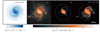Fig. 1. Face-on view of a simulated galaxy at z = 4. From left to right, the columns show the surface density of young stars (with ages ≤ 200 Myr), total gas (including H2) surface density, H2 surface density, and [C II] surface brightness. In each panel, the circle indicates 0.1 times the virial radius of the parent DM halo.

4. [C II] luminosity function

In this section, we examine the [C II] luminosity function (LF) from the MARIGOLD simulations and investigate how it evolves with redshift.

4.1. Conditional luminosity function and resolution effects

The difficulty we have to face is to combine simulations with different spatial and mass resolutions in a consistent way while accounting for sample variance given the relatively small computational volumes. For these reasons, we first performed a consistency check between the outputs of M25 and M50 by measuring the conditional luminosity function (CLF, Yang et al. 2003), i.e. the luminosity function of emitters hosted by DM halos within a narrow mass bin. Numerical simulation typically adopt a threshold of ∼100 particles to define resolved halos. Here, we have adopted a more conservative threshold of 300 DM particles for our (main) halos and examined three different cases: (i) central galaxies only, (ii) satellite galaxies only, and (iii) centrals + satellites. Our results for z = 5 and 3 are shown in Fig. 2. These cases are representative of what happens in the redshift ranges 5 ≤ z ≤ 7 and 3 ≤ z < 5, respectively.

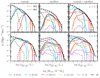Fig. 2. Conditional [C II] LF from the M25 (dashed lines) and M50 (solid lines) simulations at redshifts z = 5 and 3 for central galaxies (left panels), satellites galaxies (middle panels), and all galaxies (right panels). The coloured lines show the CLF of emitters residing in DM halos in different Mhalo bins and the black lines show the total LFs. The dotted grey line in the right panels denotes the luminosity threshold, Lthr, below which the total LFs from two simulations differ significantly due to resolution effects.

For all halo masses, the CLFs of the central galaxies in the two simulations are in excellent agreement. The CLF has a characteristic bell shape and its width grows with decreasing halo mass. Conversely, satellites have a much broader CLF and M25 presents many more faint satellites than M50 at fixed halo mass. This discrepancy reflects the different mass and spatial resolutions in the simulations that regulate the abundance of DM satellites and the [C II] emission from their gas, respectively. Inspection of the total LF reveals that the two simulations show small differences (which are compatible with sample variance) above a threshold luminosity L_thr and substantial systematic differences for $L_{[\mathrm{C}\mathrm{I}\mathrm{I}]}<L_{\mathrm{thr}}$. We find that L_thr ≃ 10^5.5 L_⊙ for 5 ≤ z ≤ 7 and L_thr ≃ 10⁸ L_⊙ for 3 ≤ z < 5 (dotted grey lines in the right panels of Fig. 2). This confirms that, as we stated before, our high-resolution M25 simulation is excellent for probing the faint end of the LF while the M50 simulation is ideally suited for probing the bright end because of its larger volume.

Finally, we note that at $L_{[\mathrm{C}\mathrm{I}\mathrm{I}]}\ge {10}^5{\mathrm{L}}_{\odot }$, the total luminosity function is fully represented by halos with masses M_halo ≥ 10⁹ h⁻¹ M_⊙. Therefore, in the following, we restrict our analysis to these ranges of luminosities and masses.

4.2. Bayesian curve fitting

At each redshift, we fitted the simulated LF, $\varphi (L_{[\mathrm{C}\mathrm{I}\mathrm{I}]})=\mathrm{d}n/\mathrm{d}log{L}_{[\mathrm{C}\mathrm{I}\mathrm{I}]}$¹, with different functional forms. Based on the discussion above, we included all galaxies with $L_{[\mathrm{C}\mathrm{I}\mathrm{I}]}\ge {10}^5{\mathrm{L}}_{\odot }$ hosted by halos with M_halo ≥ 10⁹ h⁻¹ M_⊙ from M25 but only those with $L_{[\mathrm{C}\mathrm{I}\mathrm{I}]}>L_{\mathrm{thr}}$ from M50. For the functional forms, we considered a Schechter function,

$$\begin{array}{c}\hfill \varphi (L_{[\mathrm{C}\mathrm{I}\mathrm{I}]})=ln(10){\varphi }_{\ast }{\left(\frac{L_{[\mathrm{C}\mathrm{I}\mathrm{I}]}}{L_{\ast }}\right)}^{\alpha +1}exp(-\frac{L_{[\mathrm{C}\mathrm{I}\mathrm{I}]}}{L_{\ast }}),\end{array}$$(1)

and a double power-law (DPL),

$$\begin{array}{cc}\hfill \varphi (L_{[\mathrm{C}\mathrm{I}\mathrm{I}]})=& {\displaystyle ln(10){\varphi }_{\ast }{[{\left(\frac{L_{[\mathrm{C}\mathrm{I}\mathrm{I}]}}{L_{\ast }}\right)}^{-(\alpha +1)}+{\left(\frac{L_{[\mathrm{C}\mathrm{I}\mathrm{I}]}}{L_{\ast }}\right)}^{-(\beta +1)}]}^{-1}.}\hfill \end{array}$$(2)

where all parameters have the usual meaning and β < α.

We followed a Bayesian approach and sampled the parameter space using a Markov-chain Monte-Carlo (MCMC) method implemented with the python package emcee (Foreman-Mackey et al. 2013). We assumed that the counts N_i in each logarithmic bin of luminosity follow a Poisson distribution and write the log-likelihood function for each simulation as

$$\begin{array}{c}\hfill ln\mathcal{L}={\displaystyle \sum _{i=1}^{N_{\mathrm{bins}}}}{N}_{i}ln(N_{\mathrm{model},i})-N_{\mathrm{model},i}+\mathrm{constant}.\end{array}$$(3)

Eventually, we summed the results obtained for M25 and M50.

To account for the sample variance of the simulated volumes, we followed an approach that builds upon the method originally proposed by Trenti & Stiavelli (2008) to obtain the LF from the combination of observational data with different depths. Briefly, we fitted the LF data from the two simulations with exactly the same shape but (slightly) different normalisation factors that can be written as log ϕ_*, j = log ϕ_* + Δ_j, where ϕ_* represents the ‘cosmic’ normalisation and Δ_j is the correction due to sample variance in the j^th simulation. We imposed independent Gaussian priors on each Δ_j. In other words, Δ_j ∼ 𝒩(0, (σ_v,  j/ln10)²), where σ_v,  j² is the sample variance of the overdensity within the respective simulation volume. The latter was estimated from the calculations presented in Somerville et al. (2004), considering the halo mass bin that gives the dominant contribution to the counts of emitters around L_*. We adopted (broad) flat priors on all other parameters.

As an example, we show in Appendix C, the resulting posterior distribution for the DPL fit at z = 3. In what follows, we present results obtained after marginalising the posterior distributions over the parameters, Δ_j.

Since computing the model evidence from the Markov chains is problematic, for simplicity, we used the deviance information criterion (DIC, Spiegelhalter et al. 2002) to identify whether the Schechter function or the DPL provide a better fit to the simulated data. Deviance is a measure of goodness of fit defined as D = −2lnℒ(θ), where θ indicates the parameters of a model. The DIC is obtained correcting the deviance with a penalty, p_D, for the complexity of the model which is quantified in terms of the effective number of fit parameters. There are two common approaches to estimate p_D from a Markov chain: $p_{\mathrm{D}}^{(a)}=\overline{D(\mathit{\theta })}-D(\overline{\mathit{\theta }})$ and $p_{\mathrm{D}}^{(b)}=\mathrm{Var}(D)/2$, where an overbar denotes the average over the posterior distribution (i.e. over the sampled chain) and the symbol Var denotes the corresponding variance. The DIC is then defined as DIC $=D(\overline{\mathit{\theta }})+2p_{\mathrm{D}}$. Models with smaller DIC are better supported by the data. Typically, differences (ΔDIC) above 5 are considered substantial and the model with the higher DIC is ruled out if the difference grows above 10. Based on this test, we find that the LF from our simulations is better represented by a DPL. The corresponding parameters are listed in Table 2 along with the ΔDIC values computed with both estimators for p_D. We provide in Appendix C a comparison of the two functional forms with the simulation data.

Fig. 3 shows the resulting [C II] luminosity function obtained using a DPL at different redshifts. The shaded band indicates the central 68% credibility region obtained with the MCMC method. The solid line represents the best fit (evaluated at the posterior mean $\overline{\mathit{\theta }}$). We see a clear redshift evolution in the LF. The turnover luminosity (L_*) increases (almost) monotonically with time and the faint-end slope (α) tends to flatten at late times. In contrast, the bright-end slope (β) does not show a clear evolutionary trend. The large jump in the LF at $L_{[\mathrm{C}\mathrm{I}\mathrm{I}]}\lesssim {10}^8{\mathrm{L}}_{\odot }$ is partially due to the spatial refinement that happens shortly after z = 5 in both simulations, that allows them, especially M25, to resolve more emitters. We also see a significant evolution in the number density of bright emitters. The number density of galaxies at $L_{[\mathrm{C}\mathrm{I}\mathrm{I}]}\sim {10}^9{\mathrm{L}}_{\odot }$ increases from ∼10⁻⁶ dex⁻¹ Mpc⁻³ at z = 7 to 6 × 10⁻⁴ dex⁻¹ Mpc⁻³ at z = 3, indicating a 600-fold increase in the number of L_[C II] ∼ 10⁹ L_⊙ galaxies in a less than 1.5 Gyr timespan.

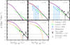Fig. 3. Simulated [C II] LF compared with observational estimates. The coloured lines represent the best-fit DPL – Eq. (2) – to the simulated LF and the shaded area represents the central 68% credibility range obtained using the MCMC chains. Black stars represent the observational estimates at z ∼ 4.5 from the ALPINE survey (Yan et al. 2020) and the grey arrow shows the lower limit from Swinbank et al. (2012) based on observations of two galaxies at z ∼ 4.4. The dashed and dotted horizontal lines represent a number count of 1 per dex in the entire simulation volume of M25 and M50, respectively. The [C II] LF from Popping et al. (2016) and Lagache et al. (2018) both based on a semi-analytical galaxy formation model, and from Garcia et al. (2024) obtained by post-processing the SIMBA simulations at z = 6 and 5 are included in the respective panels.

Observational constraints on the [C II] luminosity function at these redshifts come from Yan et al. (2020) for targeted detections at 4.5 ≲ z ≲ 5.9 in ALPINE and a lower limit at z ∼ 4.4 reported by Swinbank et al. (2012) based on [C II] detections in two observed galaxies. We find that our LFs at z = 5 and 4 are in excellent agreement with both estimates.

In Fig. 3, we also compare our [C II] LF against the results from Popping et al. (2016) and Lagache et al. (2018), both based a semi-analytical galactic formation models. Popping et al. (2016) fit a Schechter function to their predicted LFs at different redshifts. At z = 6, our predicted LF is very similar to Popping et al. (2016), despite the differences in our methods. However, deviations start to appear at late times. For instance, despite similar faint-end slopes at redshifts z = 4, our simulations predict a higher number density of emitters at the all luminosities. Moreover, our LFs extend out to higher luminosities, similar to Lagache et al. (2018), who fit their LFs with a single power law with a slope of –1.0 at all redshifts. In this regard, the underabundance of bright galaxies in semi-analytical models (SAMs) that track the H₂ abundance is a well-known problem and is related to the underabundance of cold gas in the galaxies simulated with SAMs (Popping et al. 2015). At all redshifts, we find a steeper bright-end slope in comparison to Lagache et al. (2018). We further compare with the LF from Garcia et al. (2024) obtained by post-processing the SIMBA simulations at z = 5 and 6. We find that although consistent within 1σ uncertainty, their predictions are consistently below ours and can be up to an order of magnitude lower at the bright end.

Discrepancies in the predicted LFs from different studies can have important consequences for predicting the power spectrum of the line intensity mapping (LIM) signal. LIM is an emerging technique that measures the integrated line emission from galaxies and the intergalactic medium without resolving individual sources (see Bernal & Kovetz 2022, for a recent review). The first moment of the LF governs the overall amplitude of the LIM power spectrum, while the second moment influences the shot noise component. As bright emitters are expected to have a dominant contribution to the [C II] LIM power spectrum at z ≳ 4 (e.g. Marcuzzo et al., in prep.), current and upcoming LIM surveys can prove extremely useful in constraining the different numerical models.

4.3. [C II] luminosity density

Measuring the cosmic star formation rate density (SFRD) at different epochs has been the subject of several studies (see Madau & Dickinson 2014, for a complete review). Similarly, estimating the cosmic molecular gas density from blind and targeted surveys of molecular gas tracers such as CO and dust continuum (see e.g. Walter et al. 2020; Riechers et al. 2019; Scoville et al. 2017; Magnelli et al. 2020, among others) has also gained significant interest over the last decade. Owing to the correlation between the [C II] luminosity with both the SFR and molecular gas mass across redshift, estimates of the cosmic [C II] luminosity density (ρ_[C II]) can be used to infer the cosmic SFRD and the cosmic molecular gas density (see for example, Yan et al. 2020; Loiacono et al. 2021 for the ALPINE survey and Aravena et al. 2024 for REBELS).

In Fig. 4, we show the redshift evolution of ρ_[C II] predicted by our simulations and compare with observational estimates at these redshifts. For this, we integrated the LF in Fig. 3 down to log(L_min/L_⊙) = 5. This is shown by a black line in Fig. 4 and referred to as our fiducial estimate in the following. For a fair comparison with observational estimates of ρ_[C II] from the ALPINE (Loiacono et al. 2021) and REBELS (Aravena et al. 2024) surveys, we show using red and blue lines, respectively, the ρ_[C II](z) for log(L_min/L_⊙) = 7 and log(L_min/L_⊙) = 7.5, which correspond to the luminosity cuts adopted in the two surveys for integrating the luminosity function. Note that Loiacono et al. (2021) provide two estimates for ρ_[C II] based on serendipitously detected galaxies in ALPINE at z ∼ 5; one of these is obtained by integrating the [C II] LF based on a sample of galaxies that seem to be part of a local overdensity and are therefore not representative of the galaxy population at the targeted redshift (this is referred to as the ‘clustered estimate’). The ρ_[C II] for the field population (the ‘field estimate’) can be estimated by only considering emitters detected outside the aforementioned overdensity. Since only one such emitter is detected in their sample, Loiacono et al. (2021) obtain the field estimate by multiplying the clustered estimate by the ratio between the number of emitters in the field and clustered subsamples (= 1/11), on account of the similar volumes estimated for the two subsamples. We find that the ρ_[C II] predicted by our simulations at z = 5 shows an excellent agreement with that from ALPINE for their field sample, irrespective of the luminosity cut. Conversely, as expected, the ${\rho }_{[\mathrm{C}\mathrm{I}\mathrm{I}]}^{\mathrm{clustered}}$ from ALPINE in almost an order of magnitude higher than our predicted ρ_[C II]. Our ρ_[C II] at z = 7 is lower than the REBELS one when considering their luminosity cut of 10^7.5 L_⊙ (blue line), but our ρ_[C II] with lower luminosity cuts (red and black lines) bracket the REBELS estimate. Overall, our estimates show a good agreement with observations. At z ≲ 4, the impact of a luminosity cut is not as severe.

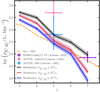Fig. 4. Comparison of the cosmic [C II] luminosity density (ρ[C II]) for different luminosity cuts in the MARIGOLD simulations with observational estimates from ALPINE (Loiacono et al. 2021) – clustered and field estimates in pink and blue, respectively; from REBELS (Aravena et al. 2024) in purple and from a semi-empirical model by Roy & Lapi (2025) shown as an orange dashed line. The ρ[C II] from the simulations is obtained by integrating the LFs shown in Fig. 3 down to log(Lmin/L⊙) = 5 (black), 7 (red), and 7.5 (blue). The shaded regions represent the 16–84 percentile range of ρ[C II] obtained from the LFs.

We also include in Fig. 4, the ρ_[C II](z) estimate from Roy & Lapi (2025), based on a semi-empirical model that performs an abundance matching of the theoretical halo mass function and the observed stellar mass function, and assigns a [C II] luminosity to every halo based on the empirical SFR-stellar-mass relation and the [C II]–SFR relation from Vallini et al. (2015). The resulting ρ_[C II](z) from their approach is similar in shape to our fiducial estimate but consistently lower by a factor of ∼2 in the redshift range shown here.

5. Correlations between intrinsic galaxy properties

Before we examine the relationship between the [C II] luminosity and the other properties of our simulated galaxies such as the SFR and the molecular gas mass (M_mol), it is instructive to inspect how these properties correlate with each other and compare them with the observed galaxy population.

In Fig. 5, we show the distribution of our simulated galaxies in the SFR-M_mol plane. The ratio of M_mol to SFR is used to define the depletion timescale τ_depl, that represents the time required to exhaust the molecular gas reservoir of the galaxy if star formation continues at the measured rate. We show lines of constant τ_depl in the figure. The observed galaxies are shown using different coloured symbols. In particular, we include the galaxies from the ALPINE survey (in light blue), the ALMA Spectroscopic Survey in the Hubble Ultra Deep Field (ASPECS, Decarli et al. 2019; Walter et al. 2020, in orange), from the Plateau de Bure High-z Blue Sequence Survey (PHIBSS Lenkić et al. 2020, in deep blue), as well as galaxies from studies by Schinnerer et al. (2016, in green) and Catán et al. (2024, pink). All observations except ALPINE obtain the M_mol based on CO rotational lines. For ALPINE, the M_mol is obtained from the observed [C II] luminosity by adopting a conversion factor α_[C II] of 31 ${\mathrm{M}}_{\odot }{\mathrm{L}}_{\odot }^{-1}$ from Zanella et al. (2018). We see that a majority of the observed galaxies have τ_depl ∼ 0.1 − 1 Gyr.

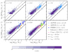Fig. 5. Distribution of the MARIGOLD galaxies in the SFR-Mmol plane at different redshifts. These are shown as purple hexbins, where the counts are sampled logarithmically.

Fig. 6 shows SFR versus M_* for the simulated galaxies at different redshifts compared with various observational estimates of the SFR–M_* relation, commonly known as the main-sequence (MS) of star-forming galaxies. Given the scatter in these relations, the distribution of our simulated galaxies in the SFR–M_* plane is consistent with the observed galaxy population at the respective redshifts.

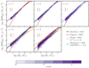Fig. 6. SFR versus M* in the MARIGOLD galaxies at different redshifts compared with observational estimates of the main-sequence (MS) of star-forming galaxies. These include the MS relations from Schreiber et al. (2015, black) and Popesso et al. (2023, red) at the respective redshifts, and the MS relations from Clarke et al. (2024, orange) based on a sample of galaxies at 2.7 ≤ z ≤ 4 and Khusanova et al. (2021, blue) based on ALPINE galaxies. The coloured errors bars on the left-hand side denote the scatter of the respective MS relations. All observed relations are extrapolated beyond the range constrained by the respective studies using a dashed line of the same colour.

6. The L_[C II]−SFR relation

We now turn our attention to investigating how the [C II] luminosity correlates with the SFR (this section) and the molecular gas mass (Sect. 7) using a statistical sample of simulated galaxies. For this, we only consider central galaxies as the [C II] LFs of the centrals from the two simulations show an excellent agreement across redshift (see the left panels of Fig. 2).

The luminosity of the [C II] line correlates strongly with the SFR in normal star-forming galaxies (Stacey et al. 2010; De Looze et al. 2014). It is one of the brightest emission lines in high-z galaxies and is unaffected by dust obscuration. Thus, it can provide an estimate of the total (unobscured+obscured) SFR in distant galaxies. Moreover, if the [C II]–SFR calibration does not evolve significantly with redshift, then it can be robustly employed across cosmic time. In this section, we aim to investigate the correlation between [C II] luminosity (L_[C II]) and the SFR in the MARIGOLD galaxies on both galaxy-wide (Sects. 6.1–6.3) and spatially resolved (Sect. 6.4) scales.

6.1. Galaxy-integrated [C II]–SFR relation

Fig. 7 shows our simulated galaxies in the L_[C II]−SFR plane for different redshifts. We calculated the SFR averaged over the last 200 Myr to be consistent with observations that commonly use a combination of SF tracers to estimate the total obscured + unobscured SF (see e.g. Kennicutt & Evans 2012; De Looze et al. 2014; Herrera-Camus et al. 2015; Lomaeva et al. 2022). For comparison, we show the best-fit relation from De Looze et al. (2014) for their high-redshift sample (0.5 ≤ z ≤ 6.6, orange solid line). We further compare with [C II]-detected galaxies at 4.4 ≲ z ≲ 5.9 from the ALPINE survey (Béthermin et al. 2020). The best-fit L_[C II]−SFR for these galaxies (Schaerer et al. 2020) is shown using a blue solid line. We also include a literature sample of [C II]-detected galaxies compiled by Olsen et al. (2015, pink symbols) and the galaxy REBELS-25 (black diamond Rowland et al. 2024) observed as part of REBELS. Many of our galaxies occupy the same region in the [C II]–SFR plane as the observed galaxies (shown as blue, pink, and black scatter points).

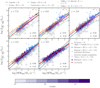Fig. 7. $[\mathrm{C}\mathrm{I}\mathrm{I}]-\mathrm{SFR}$ relation from the MARIGOLD simulations at 3 ≤ z ≤ 7 compared with observations. The simulated galaxy population is represented as purple hexbins, with the colour indicating the galaxy counts per bin. The red line showing the best-fit to these galaxies (see Table 3 for the fit parameters). In each panel, we report the Spearman’s rank correlation coefficient (ρ) and the 1σ scatter around the best-fit relation. The best-fit relation from De Looze et al. (2014) for their high−z (0.5 < z < 6.6) sample is shown in orange, with the shaded area representing the 1σ scatter. The blue line indicates the best-fit relation for 4.5 ≲ z ≲ 5.9 galaxies from the ALPINE survey (Schaerer et al. 2020). The best-fits mentioned above are extrapolated beyond the range constrained by the respective studies using a dashed line of the same colour. The individual ALPINE galaxies (at 4.5 ≲ z ≲ 5.9), the literature sample (at 5 ≲ z ≲ 7.6) taken from Olsen et al. (2015), and REBELS-25 from the REBELS survey Rowland et al. (2024) are shown with blue, pink, and black symbols, respectively. The relations from other simulations are shown as dotted lines. The relations from Lagache et al. (2018) at the respective redshift are shown in grey. The olive and cyan dotted lines along with the scatter represent the Vallini et al. (2015) relations with N = 1 and N = 3, respectively for the Kennicutt–Schmidt relation. In both cases we show the relation assuming the median Zgas of our simulated galaxies at a given redshift. The pink and teal lines represent the relations from Leung et al. (2020) and Vizgan et al. (2022), respectively, both obtained by post-processing the z ∼ 6 snapshot of the SIMBA simulations (Davé et al. 2020) with different versions of SíGAME (Olsen et al. 2015, 2017). The grey line represents the relation from Casavecchia et al. (2024).

At each redshift, we fitted a relation of the form $\log (L_{[\mathrm{C}\mathrm{I}\mathrm{I}]}/{\mathrm{L}}_{\odot })=a\log ({\mathrm{SFR}}_{200}/{\mathrm{M}}_{\odot }{\mathrm{yr}}^{-1})+b$ (where {a, b}∈ℝ²) to our simulated galaxies using an ordinary least squares linear regression (shown as a solid red line in Fig. 7). We report in Table 3 the resulting parameters along with the 1σ dispersion, where σ is the standard deviation of the residuals around the best fit in each case.

Firstly, from the distribution of simulated galaxies at different redshifts in the [C II]–SFR plane, we immediately see an increase in L_[C II] at a given SFR from z = 7 to z = 3. At z = 3, our galaxies are well-distributed around the De Looze et al. (2014) relation and our best fit is in excellent agreement with theirs, while at z = 4, we obtain a similar relation as Schaerer et al. (2020) (considering conservative upper limits on [C II] non-detections to the ALPINE galaxy sample). The value of the Spearman’s rank correlation coefficient, indicated in each panel in Fig. 7, increases with time and remains high (≳0.86) at all redshifts. We further find that the scatter L_[C II]−SFR relation increases with increasing redshift, similar to previous findings by Carniani et al. (2018) for a sample of ∼50 galaxies at 5 ≲ z ≲ 7. In contrast, based on a semi-analytical galaxy formation model coupled to the spectral synthesis code CLOUDY (Ferland et al. 1992), Lagache et al. (2018) reported a slight decrease in the scatter of the L_[C II]−SFR relation with redshift.

6.2. Redshift evolution of the $[\mathrm{C}\mathrm{I}\mathrm{I}]-\mathrm{SFR}$ relation

An important question concerning the [C II]–SFR relation is whether it shows any evolution with redshift. For instance, based on the ALPINE survey, Schaerer et al. (2020) found that star-forming galaxies at 4 ≲ z ≲ 6 follow the same or a slightly steeper [C II]–SFR relation compared to local galaxies (De Looze et al. 2014, shown as an orange line in Fig. 7), depending on the treatment of non-detections in their galaxy sample. For the MARIGOLD galaxies, the slope of the L_[C II]−SFR relation shows little redshift evolution in the range 3 ≤ z ≤ 7 (≲ 0.15 dex variation). As noted before, the best fit for our lowest redshift galaxy sample (z = 3) is in excellent agreement with the De Looze et al. (2014), but deviations towards lower L_[C II] are evident at z ≳ 5. Consequently, at a given SFR, L_[C II] decreases with increasing redshift. This is reflected in the monotonically increasing values of the intercept b from z = 7 to z = 3 (see Table 3), which increases by a factor of ∼3 (0.5 dex) in this redshift range. To conclude, we find a redshift evolution in the intercept of the [C II]–SFR relation, as evident from the offset between our best-fit relation and the De Looze et al. (2014) relation that is the same in all panels.

6.3. Comparison with previous work

In Fig. 7, we also compare our best-fit [C II]–SFR relation (Table 3) with previous numerical work in the literature, briefly described in the following. Lagache et al. (2018) used a semi-analytical galaxy-formation model coupled to the photoionisation code CLOUDY (Ferland et al. 1992) to obtain the [C II] luminosity for a statistical sample of galaxies at redshifts 4 ≤ z ≤ 8. From their full sample of galaxies, they obtain a [C II]–SFR relation of the form: $\log (L_{[\mathrm{C}\mathrm{I}\mathrm{I}]}/{\mathrm{L}}_{\odot })=(1.4-0.07z)\log (\mathrm{SFR}/{\mathrm{M}}_{\odot }{\mathrm{yr}}^{-1})+7.1-0.07z$, which is shown as solid lime line in the figure. Vallini et al. (2015) calculated the [C II] emission from a single z ∼ 7 galaxy from a high-resolution (≈60 pc) SPH simulation (Pallottini et al. 2014) assuming optically thin emission. To do so, they adopt a log-normal sub-grid density distribution with a variable Mach number. In this regard, their approach is similar to ours except that we adopt a log-normal+power-law PDF in regions where self-gravity cannot be neglected (see Khatri et al. 2024, for details). They investigate how the total [C II] luminosity changes with metallicity, assuming a uniform metal distribution. To derive the [C II]–SFR relation, they scale the [C II] luminosity with the molecular gas mass ($L_{[\mathrm{C}\mathrm{I}\mathrm{I}]}\propto M_{{\mathrm{H}}_2}$), which is assumed to scale with the SFR in accordance with the Kennicutt-Schmidt relation: Σ_SFR ∝ Σ_H2^N. In Fig. 7, we show their results for N = 1 and N = 2. For both cases, the dotted line is for the median gas-metallicity (Z_gas) of our galaxies at a given redshift.

Previously, Lagache et al. (2018) found that their [C II]–SFR agrees well with the one from Vallini et al. (2015) for N = 2. We also include the results from Leung et al. (2020) and Vizgan et al. (2022), both of which were obtained by post-processing z ∼ 6 galaxies from the SIMBA simulations using different versions of the emission line tool SíGAME (Olsen et al. 2015, 2017). SíGAME includes a multi-phase ISM model and accounts for the contribution of different phases (molecular gas phase, cold neutral medium, and H II regions) to the [C II] emission of a galaxy and employs CLOUDY to obtain the chemical abundances in the different phases. The relation from Casavecchia et al. (2024) is obtained by post-processing z ≥ 6 galaxies from the COLDSIM simulations.

Overall, we see that the variation among the different models increases with redshift, and can span up to an order of magnitude at SFR ∼ 1 − 10 M_⊙ yr⁻¹. This is enhanced towards lower and higher SFRs. We find that at all redshifts our [C II]–SFR relation differs significantly from Vallini et al. (2015). In this regard, while their approach for calculating the [C II] emission accounting for the sub-grid densities is similar to ours (albeit with different sub-grid density PDFs), their method to derive the [C II]–SFR relation relies on scaling relations between L_[C II] and M_H2 and Σ_SFR − Σ_H2, while we follow the dynamical evolution of these quantities in our simulations. Moreover, as shown by our PCA analysis (Sect. 7.2), the L_[C II]−M_mol relation exhibits a secondary dependence on the SFR that evolves with redshift. This provides a natural explanation for the different results from the two studies. At 5 ≤ z ≤ 7, our results, as well as those from Lagache et al. (2018), show slightly steeper slopes compared to those from Leung et al. (2020) and Vizgan et al. (2022). However, these differences remain within the scatter of ∼0.3 − 0.6. Notably, at these redshifts, the numerical predictions fall slightly below the empirical De Looze et al. (2014) relation. At z = 3, our best-fit shows an excellent agreement with De Looze et al. (2014) and exhibits a slightly higher offset compared to others except Lagache et al. (2018).

6.4. Spatially resolved $[\mathrm{C}\mathrm{I}\mathrm{I}]-\mathrm{SFR}$ relation

Resolved observations of [C II] and SF in high-redshift galaxies have found that these galaxies exhibit a “[C II] deficit” with respect to the local Σ_[C II] − Σ_SFR relation. For example, Carniani et al. (2018) found that the galaxy-integrated [C II]–SFR relation at 5 ≲ z ≲ 7 is similar to the local one but in the ${\mathrm{\Sigma }}_{[\mathrm{C}\mathrm{I}\mathrm{I}]}-{\mathrm{\Sigma }}_{\mathrm{SFR}}$ plane, the galaxies have a substantially lower ${\mathrm{\Sigma }}_{[\mathrm{C}\mathrm{I}\mathrm{I}]}$ compared to the local galaxies at any given Σ_SFR. They attributed the offset mainly to the lower metallicity of these galaxies and stressed that the more extended [C II] emission in high-z galaxies could also play a role.

Here we examine the (spatially resolved) Σ_[C II] − Σ_SFR relation in our simulated galaxies. For simplification, we present results based on z = 4 galaxies only. In each galaxy, the [C II] surface brightness and SFR surface density are obtained from a face-on projection of a cube centred on the galaxy and of side length equal to twice the size of the galaxy. The spatial resolution (minimum grid cell size; see Table 1) of our simulations is better than that achieved in current high-z [C II] observations that can resolve kpc-scale regions within z ≳ 4 galaxies (e.g., Posses et al. 2024). Therefore, we applied a 2D Gaussian smoothing to our simulated surface brightness and surface density maps to mimic observations. For this analysis, we adopted the beam sizes (in terms of the full-width at half-maximum, FWHM) for the SFR surface density and the [C II] surface brightness measurements from Posses et al. (2024), which are 0.2″ and 0.17″, respectively. At z = 4, these correspond to ∼1.4 kpc and ∼1.2 kpc.

In the left panel of Fig. 8, we show the Σ_[C II] − Σ_SFR relation for our simulated galaxies. We split our simulated galaxies into three groups according to their stellar mass (M_*), with the number of galaxies in each group indicated in the legend. For each group, solid lines show the median ${\mathrm{\Sigma }}_{[\mathrm{C}\mathrm{I}\mathrm{I}]}$ as a function of Σ_SFR and the shaded area represents the interquartile range. The median ${\mathrm{\Sigma }}_{[\mathrm{C}\mathrm{I}\mathrm{I}]}$ shows slight variations among the different M_* bins. Most notably, towards higher Σ_SFR, lower M_* galaxies exhibit a lower ${\mathrm{\Sigma }}_{[\mathrm{C}\mathrm{I}\mathrm{I}]}$, likely because of their (relatively) low metallicity. The median ${\mathrm{\Sigma }}_{[\mathrm{C}\mathrm{I}\mathrm{I}]}$ in all M_* bins is lower than the local relation and similar to the relation from Schaerer et al. (2020, same as in Figure 12 of Posses et al. 2024).

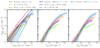Fig. 8. Spatially resolved $[\mathrm{C}\mathrm{I}\mathrm{I}]-\mathrm{SFR}$ relation for the MARIGOLD galaxies at z = 4. The galaxies are divided into different stellar-mass bins (the number of galaxies in each bin is indicated in the legend). The solid lines show the median ${\mathrm{\Sigma }}_{[\mathrm{C}\mathrm{I}\mathrm{I}]}$ as a function of the SFR surface density (left), of the gas surface density (middle), and of the H2 surface density (right). The shaded areas represent the 16–84 percentile range. In the left panel, dashed lines indicate the empirical relations from De Looze et al. (2014, red) based on local dwarf galaxies from the Herschel Dwarf Galaxy Survey, for ALPINE galaxies in black (based on global values only Schaerer et al. 2020, black), and for a sample of galaxies at 5 < z < 7.2 from Carniani et al. (2018, teal). For the simulated galaxies, the [C II] surface brightness, and the SFR, gas, and H2 surface densities were obtained from a face-on projection of a cube centred on the galaxy and of side length equal to twice the radius of the galaxy.

At Σ_SFR ≲ 1 M_⊙ yr⁻¹ kpc⁻², our medians for all M_* bins are consistent with the Schaerer et al. (2020) relation, but at higher Σ_SFR, they start to deviate towards lower ${\mathrm{\Sigma }}_{[\mathrm{C}\mathrm{I}\mathrm{I}]}$ values and the shaded area overlaps with the Carniani et al. (2018). This trend continues towards higher Σ_SFR, and for Σ_SFR ≳ 10 M_⊙ yr⁻¹ kpc⁻², the median ${\mathrm{\Sigma }}_{[\mathrm{C}\mathrm{I}\mathrm{I}]}$ from our simulations is lower than the Schaerer et al. (2020) and Carniani et al. (2018) relations by a factor of ≈2.5.

For the same galaxies, we also show the ${\mathrm{\Sigma }}_{[\mathrm{C}\mathrm{I}\mathrm{I}]}-{\mathrm{\Sigma }}_{\mathrm{gas}}$ and ${\mathrm{\Sigma }}_{[\mathrm{C}\mathrm{I}\mathrm{I}]}-{\mathrm{\Sigma }}_{{\mathrm{H}}_2}$ in Fig. 8. The gas surface densities are smoothed with a Gaussian beam of FWHM of ∼1.2 kpc (same as for ${\mathrm{\Sigma }}_{[\mathrm{C}\mathrm{I}\mathrm{I}]}$).

Once again, there are no strong variations among the different M_* bins except at the highest gas surface densities. In the ${\mathrm{\Sigma }}_{[\mathrm{C}\mathrm{I}\mathrm{I}]}-{\mathrm{\Sigma }}_{{\mathrm{H}}_2}$ plane, a similar trend is observed although with larger differences, similar to those in the Σ_[C II] − Σ_SFR plane. We also observe that in all panels, the slope decreases towards higher surface densities.

6.5. Possible [C II]-deficit?

At Σ_SFR ≳ 1 M_⊙ yr⁻¹ kpc⁻², our Σ_[C II] − Σ_SFR relation deviates from the Schaerer et al. (2020) relation towards lower ${\mathrm{\Sigma }}_{[\mathrm{C}\mathrm{I}\mathrm{I}]}$ and exhibit values similar to the Carniani et al. (2018) relation, albeit with a shallower slope. As regions of high SF are expected to be rich in dust and thereby bright in FIR emission, this trend is similar to the observed ‘[C II]-deficit’, that is to say, the decrease in the ratio of the [C II] to the FIR luminosity in luminous infrared galaxies.

We investigated the underlying cause of this deficit by examining the surface density of C⁺, and CO as a function of Σ_SFR, Σ_gas, and the surface density of metals (Σ_metals) in our galaxies in Appendix D. We see that Σ_C⁺ plateaus towards high Σ_SFR and Σ_gas, while Σ_CO continues to grow. This happens for two reasons: firstly, a high Σ_gas leads to a higher H₂ abundance. Second, a higher Σ_SFR is associated with a higher dust abundance; together these provide better shielding of CO against the dissociating UV radiation in dense environments. Therefore, in regions with a high SFR surface density, the bulk of the carbon is locked up in CO, leading to a flattening of Σ_C⁺ towards high Σ_SFR, and consequently a slower increase of the [C II] surface brightness towards high SFR and gas surface densities. Further note that our simulations do not account for the UV radiation from active galactic nuclei (AGN), that can contribute to the first ionisation of carbon (and subsequently to [C II] emission). While some studies suggest that AGN are not a significant source of [C II] emission (see for example, De Breuck et al. 2022), their contribution has not yet been estimated using a large sample of galaxies at high redshifts. However, the harder ionizing radiation from AGN can also ionize C⁺, resulting in a decrease in the [C II] emission (Langer & Pineda 2015). In this case, the [C II] luminosity could be even lower than predicted by our model.

A similar decline in [C II] was also reported by De Looze et al. (2014) (see their Figure 2) who found that the slope of the ${\mathrm{\Sigma }}_{\mathrm{SFR}}-{\mathrm{\Sigma }}_{[\mathrm{C}\mathrm{I}\mathrm{I}]}$ relation steepens for ${\mathrm{\Sigma }}_{[\mathrm{C}\mathrm{I}\mathrm{I}]}\gtrsim$ few times ${10}^6{\mathrm{L}}_{\odot }{\mathrm{kpc}}^{-2}$ indicating that the [C II] line is not the dominant coolant in intensely star-forming regions. Such a deficit would manifest as a shallower slope of the Σ_[C II] − Σ_SFR relation towards higher ${\mathrm{\Sigma }}_{[\mathrm{C}\mathrm{I}\mathrm{I}]}$ (and higher Σ_SFR).

Overall we find that for our simulated galaxies at z = 4, the median ${\mathrm{\Sigma }}_{[\mathrm{C}\mathrm{I}\mathrm{I}]}$ in a given Σ_SFR bin shows an excellent agreement with the best-fit to ALPINE galaxies at 4.4 ≤ z ≤ 5.9 for Σ_SFR ≲ 1 M_⊙ yr⁻¹ kpc⁻². Towards higher Σ_SFR, however, the median shows a flattening. This is driven by the increased abundance of CO at the expense of C⁺ along high surface density lines of sight.

7. [C II] emission as a molecular gas tracer

Zanella et al. (2018) identified a strong correlation between the luminosity of the [C II] line and the molecular gas mass based on a compilation of galaxies in the redshift range 0 ≤ z ≤ 5.5. Their sample includes local dwarf galaxies, main-sequence galaxies at 0 ≤ z ≤ 5.5, starburst galaxies at 0 ≲ z ≲ 2 and local luminous/ultra-luminous infrared galaxies. The best fit to their galaxy sample is given by:

$$\begin{array}{c}\hfill \log \left(\frac{L_{[\mathrm{C}\mathrm{I}\mathrm{I}]}}{{\mathrm{L}}_{\odot }}\right)=-1.28(\pm 0.21)+0.98(\pm 0.02)\log \left(\frac{M_{\mathrm{mol}}}{{\mathrm{M}}_{\odot }}\right),\end{array}$$(4)

with a scatter of ≈0.3 dex around the best fit. Consequently, [C II] emission is now routinely used as a molecular gas tracer in high-redshift galaxies and it seems to be as good as conventional tracers like CO rotational lines and dust continuum emission. For instance, Dessauges-Zavadsky et al. (2020) found that the [C II]-based molecular gas mass estimates for ALPINE galaxies were consistent with those derived from dynamical mass estimates and (rest-frame) infrared luminosities. Aravena et al. (2024) found similar results for REBELS galaxies at 6.5 ≲ z ≲ 7.5.

However, this relation and its redshift evolution have not been extensively explored in numerical simulations. While Vizgan et al. (2022) investigated the [C II]–M_mol relation in SIMBA simulations at a specific redshift of z ∼ 6, a detailed study at different epochs is still lacking. To address this, here we examine the [C II]-molecular gas connection in the MARIGOLD galaxies at different redshifts and develop a prescription for inferring the molecular gas mass of a galaxy from its [C II] emission. In Fig. 9, we compare the L_[C II]−M_mol relation for our simulated galaxies at different redshifts against the calibrations from Zanella et al. (2018), Madden et al. (2020), and Vizgan et al. (2022).

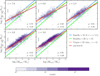Fig. 9. [C II]−Mmol relation from our simulations compared with observations. The simulated galaxies are represented by purple hexbins, where the colour indicates the number of galaxies in each bin. The solid red line gives the ordinary least squares linear fit to these galaxies, with the fit parameters listed in Table 3. In each panel, we report the Spearman’s rank correlation coefficient (ρ) and the 1σ scatter around the best-fit relation. The best fit to the observed galaxy sample at z = 0 − 5.5 by Zanella et al. (2018) is shown in blue and the fit to the z ∼ 0 dwarf galaxies (Madden et al. 2020) is shown in lime. The relation from SIMBA simulations at z = 6 (Vizgan et al. 2022) is shown in orange. As in Fig. 7, the extrapolated Zanella et al. (2018) relation is shown as a dashed line of the same colour.

The molecular gas mass, M_mol, was obtained by scaling up the H₂ mass directly obtained from the simulations by 1.36 to account for the contribution of helium and heavier elements confined with H₂. At each redshift, we performed an ordinary least squares regression to fit a linear relation of the form: $\log (L_{[\mathrm{C}\mathrm{I}\mathrm{I}]})=a\log (M_{\mathrm{mol}})+b$ to our galaxies. The corresponding best-fit parameters and the 1σ dispersion around the best fit are listed in Table 3. We observe that the slope increases with time from z = 7 to z = 4 and thereafter decreases slightly (by ≈0.04 dex). The overall change of ≈0.2 dex in the slope between z = 7 and z = 3 is similar to the change of ≈0.15 dex in the slope of the $[\mathrm{C}\mathrm{I}\mathrm{I}]-\mathrm{SFR}$ relation. At all redshifts, our best-fit slope is shallower than that of the Zanella et al. (2018) relation. As a result only our high-mass (M_mol ≳ 10⁹ M_⊙) galaxies follow their relation, while our low-mass galaxies exhibit higher L_[C II] than expected from extrapolation of their relation.

We also report in Fig. 9, the Spearman’s rank correlation coefficient (ρ) between L_[C II] and M_mol at each redshift. From the monotonically increasing values of ρ across redshift, we see that the [C II]–M_mol correlation is relatively weak at z ≳ 5 and becomes progressively stronger over time. This is in contrast with the [C II]–SFR correlation that exhibits a high value (ρ ≳ 0.86) out to z = 7. This trend is also evident from the decreasing values of the scatter (σ) around the best-fit linear relation between L_[C II] and M_mol with decreasing redshift.

7.1. The conversion factor α_[C II]

Next we computed the conversion factor between the [C II] luminosity and the molecular gas mass: α_[C II]. Fig. 10 shows the probability distribution function of the α_[C II] exhibited by the MARIGOLD galaxies. We see that at all redshifts, log log α_[C II] exhibits a skewed distribution with an extended tail towards higher values. The tail is particularly prominent at high redshifts. However, the scatter reduces towards lower redshifts. The peak α_[C II] at these redshifts lies in the range 7–24 ${\mathrm{M}}_{\odot }{\mathrm{L}}_{\odot }^{-1}$ and increases with redshift.

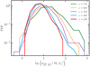Fig. 10. Probability distribution function of the conversion factor α[C II] exhibited by our simulated galaxies at different redshifts.

Fig. 11 shows the correlation between α_[C II] and various galaxy properties for our simulated galaxies, namely the gas-phase metallicity, $12+\log (\mathrm{O}/\mathrm{H})$, the SFR averaged over the last 5 Myr (SFR₅), the SFR averaged over the last 200 Myr (SFR₂₀₀), and the ratio of the SFRs averaged over the last 5 and 200 Myr (hereafter R_{5 − 200}). The use of the latter is motivated by Lomaeva et al. (2022), who proposed an SFR change diagnostic derived from the ratio of SFR₅ and SFR₂₀₀ to quantify the current rate of change of the SFR. As different SFR indicators are sensitive to the SF happening on different timescales, their ratio can be used to quantify the SFR change over time. Lomaeva et al. (2022) proposed the ratio of $\mathrm{H}\alpha$ to FUV emission as a proxy for SFR₅/SFR₂₀₀. This quantity has also been used recently to quantify the bursty SF in galaxies observed with the James Webb Space Telescope (see for example, Atek et al. 2024; Clarke et al. 2024).

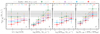Fig. 11. Conversion factor α[C II] in our simulated galaxies as a function of gas metallicity (panel a), the SFR averaged over the last 5 Myr (panel b), the SFR averaged over the last 200 Myr (panel c), and the SFR change diagnostic R5 − 200 (panel d, see text) at different redshifts. The coloured symbols represent the median α[C II] in each bin, while the error bars represent the 16–84 percentiles. The Spearman’s rank correlation coefficient between the variables on the y and x axes are shown in each panel as well. The grey dotted line denotes the mean α[C II] from Zanella et al. (2018) and the shaded band represents the corresponding scatter.

In each panel of Fig. 11, we show the median α_[C II] in different bins of the quantity on the x-axis along with the 16–84 percentile range (denoted by error bars). Firstly, we observe that the α_[C II] values span about two orders of magnitude at all redshifts, particularly at z ≥ 6. The Spearman’s rank correlation coefficient (denoted by ρ) for the galaxy sample at different redshifts is reported in each panel. We find a weak correlation between α_[C II] and gas metallicity at all redshifts and observe a large scatter at all values of 12 + log(O/H), in agreement with Zanella et al. (2018) who found little systematic variation of α_[C II] with metallicity.

In panel b of Fig. 11, we observe that α_[C II] increases with SFR₅ at all redshifts, with the highest variation occurring at z = 7. At SFR ≳10 M_⊙ yr⁻¹, our α_[C II] values at all redshifts are in good agreement with the range from Zanella et al. (2018), but deviate towards lower values at lower SFRs. Therefore, using a constant α_[C II] (calibrated on the high-SFR galaxies alone) would lead to an overestimate of the molecular gas mass in low-SFR galaxies. A similar trend is observed between α_[C II] and SFR₂₀₀ in panel c. However, the strength of the correlation between this pair of variables is much lower than the previous, as indicated by the lower values of ρ. This shows that the conversion factor depends strongly on the SFR averaged over a small timescale and less so on the SFR averaged over a longer timescale.

Finally, in panel d, we see that α_[C II] increases with R_{5 − 200}, with ρ ∈ [0.68, 0.83]. Interestingly, in this case the correlation is the strongest at high redshifts and slowly decays at lower redshifts, highlighting the increased sensitivity of α_[C II] on the star-formation history of galaxies at z ≳ 6, as quantified by SFR change parameter R_{5 − 200}.

We note however that observations of starburst galaxies at z ∼ 4 from Rizzo et al. (2021) exhibit lower α_[C II] than the Zanella et al. (2018) calibration. These galaxies have ${\alpha }_{[\mathrm{C}\mathrm{I}\mathrm{I}]}\sim 5-19{\mathrm{M}}_{\odot }{\mathrm{L}}_{\odot }^{-1}$, despite having SFRs in excess of 100 M_⊙ yr⁻¹. This is in contrast to our finding of α_[C II] increasing with the SFR. A comparison of the molecular gas mass and depletion timescale of Rizzo et al. (2021) and our galaxies shows that four out of five of the Rizzo et al. (2021) galaxies have an order of magnitude lower τ_depl (≲ 0.02 Gyr) compared to our galaxies with similar masses (M_mol ≥ 10¹⁰ M_⊙, see Fig. 5), indicating a faster consumption of molecular gas in these galaxies compared to the MARIGOLD galaxies.

7.2. Secondary dependence of the [C II]–M_mol relation

After examining how α_[C II] varies with other galaxy properties, we developed a prescription for inferring the molecular gas mass of a galaxy from its [C II] emission, taking into account these secondary dependences. For this, we performed a principal component analysis (PCA) in the 5D space of parameters – M_mol, L_[C II], SFR₅, SFR₂₀₀ and 12 + log(O/H). PCA identifies dominant patterns and correlations between the parameters, reducing the dimensionality while approximately preserving variance. This technique has been previously used to identify secondary dependencies in the stellar-mass-metallicity relation on SFR and other parameters (Mannucci et al. 2010; Lara-López et al. 2010; Hunt et al. 2012; Bothwell et al. 2016).

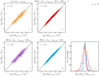Fig. 12. Comparison of the predicted molecular gas mass estimates with the true molecular gas mass using two different approaches for simulated galaxies at z = 4. Panel a shows the performance of the best-fit relation between Mmol and L[C II], while panels b–d present results from different PCA-based relations (as indicated in the title of each panel). The corresponding relations are listed in Table 5. In panels a–d, the top-left corner reports σ, the standard deviation of the offset between the predicted and true Mmol (both in log scale). Panel e compares the distributions of these offsets from the different approaches.

Since PCA is highly sensitive to extremes in the data, we first scaled all parameters by their respective mean and standard deviation before performing the analysis such that for a parameter X,

$$\begin{array}{c}\hfill \stackrel{\sim }{X}=\frac{\log X-⟨\log X⟩}{\sqrt{\mathrm{variance}(\log X)}}\end{array}$$(5)

denotes the scaled variable.

The results of this analysis at z = 4 are shown in Table 4. About 88% of the variance is explained by the first principal component and ∼95% is explained by the first two principal components. The first component contains nearly equal contributions from all variables, while PC2 is dominated by metallicity. The last principal component, PC5 is dominated by M_mol while containing only 0.35% of the sample variance. Therefore, we set PC5 to zero and renormalize to obtain an expression for M_mol in terms of the other quantities:

$$\begin{array}{cc}\hfill \log (M_{\mathrm{mol}}/{\mathrm{M}}_{\odot })& =4.11+0.47\log (L_{[\mathrm{C}\mathrm{I}\mathrm{I}]}/{\mathrm{L}}_{\odot })\hfill \\ \hfill & +0.59\log ({\mathrm{SFR}}_5/{\mathrm{M}}_{\odot }{\mathrm{yr}}^{-1})\hfill \\ \hfill & +0.01\log ({\mathrm{SFR}}_{200}/{\mathrm{M}}_{\odot }{\mathrm{yr}}^{-1})\hfill \\ \hfill & +0.09[12+log(O/H)].\hfill \end{array}$$(6)

The M_mol obtained from Eq. (6) versus the true M_mol is shown in Fig. 12. We also contrast this with the M_mol obtained from the best-fit relation between M_mol and L_[C II]². The latter shows ≈2.3 times higher scatter. The 1σ standard deviation between the true M_mol and the predicted M_mol using the PCA-based relation is 0.13 implying that for most (95%) of the galaxies, the PCA relation predicts the true molecular gas mass within a factor of ∼1.8 while using the two variable linear best-fit, the molecular gas mass is predicted within a factor of 4. It is worth noting that while the linear relation systematically underpredicts M_mol for M_mol ≳ 10¹⁰ M_⊙ (as the linear fit is heavily influenced by the more numerous low-mass galaxies), the PCA-based prediction does not suffer from this discrepancy.

We obtain similar results at other redshifts; these are listed in Table 5. To estimate the uncertainties in the coefficients of the PCA-based relation, we performed a bootstrapping analysis with replacement, using 1000 iterations at each redshift. We find that the coefficient a, that quantifies the dependency of M_mol on L_[C II], increases from z = 6 to z = 3, while the coefficient b, that represents the dependency of M_mol on SFR₅ decreases such that at z = 3, a ≈ b. Interestingly, the dependence of M_mol on SFR₂₀₀ and metallicity is relatively low at all times and does not evolve significantly with redshift.

Based on this finding, we inspect the efficacy of a simpler PCA-based relation namely using three variables: M_mol, L_[C II], and SFR₂₀₀ as well as M_mol, L_[C II], and SFR₅. A comparison of the M_mol obtained this way against the true molecular gas mass is presented in panels c and d of Fig. 12. The resulting relations at all redshifts are listed in Table 5. Across redshift, we find that the $M_{\mathrm{mol}}-L_{[\mathrm{C}\mathrm{I}\mathrm{I}]}-{\mathrm{SFR}}_5$ relation offers a similar level of accuracy as the 5-variable PCA-based relation, while being more convenient to use from an observational point of view. In contrast, the $M_{\mathrm{mol}}-L_{[\mathrm{C}\mathrm{I}\mathrm{I}]}-{\mathrm{SFR}}_{200}$ relation does not provide a significant gain compared to the best-fit $M_{\mathrm{mol}}-L_{[\mathrm{C}\mathrm{I}\mathrm{I}]}$ relation (panel a of Fig. 12).

7.3. Accounting for observational uncertainties

To estimate the impact of observational uncertainties in measurements of L_[C II], SFR₅, SFR₂₀₀, and 12 + log (O/H) in estimating M_mol, we added a random perturbation, δ, to each of the four quantities, where δ was drawn from a normal distribution with a mean of zero and a standard deviation corresponding to the typical errors reported in observations of high-z galaxies. For instance, we adopted an error of 0.1 dex for L_[C II] and 0.24 dex for SFR₅ and SFR₂₀₀, both based on ALPINE galaxies (Béthermin et al. 2020). For 12 + log(O/H), we adopted an error of 0.05 dex (Sanders et al. 2015). Then we employed the PCA-based relations shown in Table 5 to obtain a prediction for M_mol and computed the offset between our prediction and the true M_mol (as before, the offset is computed from the log of the quantities). We then computed the standard deviation of this offset. We repeated the procedure for the best-fit $M_{\mathrm{mol}}-L_{[\mathrm{C}\mathrm{I}\mathrm{I}]}$ relation. The resulting σ values are reported in the last two columns of Table 5. Overall, we found that even accounting for observational uncertainties, the PCA-based relation provides a significant gain in the precision/accuracy of molecular gas mass estimates and is capable of predicting the true molecular gas mass within a factor of 3 at 3 ≤ z ≤ 6.

7.4. Correlation with other quantities

In addition to the SFR and the molecular gas mass, the [C II] emission at high redshifts has been shown to correlate with the metal mass in the gas-phase of high-z galaxies (Heintz et al. 2023). In Khatri et al. (2024), we found that the C⁺ distribution in our post-processed galaxy shows a grater similarity with the total gas distribution while CO and atomic carbon correlate better with the molecular gas. Inspired by these findings, we further investigated the correlation between L_[C II] and the total gas mass (M_gas) and the mass in metals (M_metal). At each redshift, we performed an ordinary least squares regression and the resulting parameters and the 1σ scatter around the best fit are listed in Table 6.

We find that among the galaxy properties explored so far, namely the SFR, the molecular gas mass, the total gas mass, and the metal mass, the [C II] emission in our simulated galaxies shows the strongest/tightest correlation with M_metal across redshifts. This is evident from the lowest scatter in this relation. In other words, we can say that the [C II] luminosity is the best predictor of the gas-phase metal mass in any given galaxy. Interestingly, the scatter in the $L_{[\mathrm{C}\mathrm{I}\mathrm{I}]}-M_{\mathrm{metal}}$ relation is lower than the scatter in the $L_{[\mathrm{C}\mathrm{I}\mathrm{I}]}-M_{\mathrm{gas}}$ relation at all times. A strong correlation between [C II] emission and total gas mass simply highlights the multi-phase origin of the emission.

After exploring the correlation between L_[C II] and other galaxy properties in our simulations, we now turn our attention to examining the spatial extent of the [C II] emission in these galaxies and how it varies across the galaxy population.

8. Extended [C II] emission

In recent years, several observations of high-z (z ≳ 4) galaxies have revealed that the [C II] emission extends 2–3 times farther than the UV continuum emission. These findings come from both stacked galaxy samples (e.g., Fujimoto et al. 2019; Ginolfi et al. 2020; Fudamoto et al. 2022) and individual galaxies (e.g., Fujimoto et al. 2020; Lambert et al. 2023; Posses et al. 2024), with some studies, like Posses et al. (2024), resolving emission on ∼1 kpc scales within galaxies. Potential sources of this extended emission include unresolved satellites, outflows, and extended PDRs (see, for example, Figure 12 in Fujimoto et al. 2019). In Khatri et al. (2024), we examined the extent of C⁺ in a simulated galaxy by calculating the H₂, CO, C, and C⁺ abundances in post-processing using the sub-grid model HYACINTH, and found that the C⁺ surface density profile is more extended than other components such as H₂ and CO, and closely resembles the total gas distribution and that of young stars (with ages ≤ 20 Myr). In this paper, we extended our analysis to a statistical sample of galaxies from the MARIGOLD suite and examined the extent of their [C II] emission. For this, we first looked at the stacked emission from a sample of galaxies at two different redshifts (Sect. 8.1). Then we inspected the relative extent of the [C II] emission with respect to SF in individual galaxies and investigate possible causes of an extended [C II] emission (Sect. 8.2).

8.1. Stacked [C II] emission

First, we compared the stacked [C II] emission from our simulated galaxies with that from Ginolfi et al. (2020), based on 50 [C II]-detected galaxies from ALPINE at z = 4.5 − 5.9. The stacked [C II] emission from these galaxies extends out to ∼15 kpc. The authors further split their sample into low star-forming (SFR < 25 M_⊙ yr⁻¹) and high star-forming (SFR ≥ 25 M_⊙ yr⁻¹) galaxies and reported that the extended [C II] emission is more prominent in the latter.

To compare with these observations, we selected galaxies at redshifts z = 4 and z = 5 with M_* and SFR in the range exhibited by the Ginolfi et al. (2020) sample, that is, 10^9.25 M_⊙ ≤ M_* ≤ 10^11.25 M_⊙ and 5 M_⊙ yr⁻¹ ≤ SFR ≤ 600 M_⊙ yr⁻¹. We note that while the Ginolfi et al. (2020) sample includes galaxies with SFR up to 600 M_⊙ yr⁻¹, the highest SFR in our sample is ∼300 M_⊙ yr⁻¹ at z = 4 and ∼170 M_⊙ yr⁻¹ at z = 5. Following Ginolfi et al. (2020), we further split our simulated galaxies into low-SFR (SFR <  25 M_⊙ yr⁻¹) and high-SFR (SFR ≥ 25 M_⊙ yr⁻¹) samples.

For each galaxy, we obtained the [C II] surface brightness map from the 2D projection of a cylinder centred on the galaxy with a line-of-sight velocity cut of v_los ∈ [−200,200] km s⁻¹ (same as in Ginolfi et al. 2020) along three orthogonal lines of sights (these are taken to be the coordinate axes of the simulation box). Note that in this analysis, we adopted the stellar centre of the galaxy to be the spatial centre of the [C II] emission³. We smoothed the resulting surface brightness maps with a 2D Gaussian beam of FWHM 0.9″ to mimic the synthesised ALMA beam in Ginolfi et al. (2020). We then stacked the individual smoothed surface brightness maps. Note that, since we do not add noise to the galaxy images, our stacking procedure is unweighted by construction and is different from the variance-weighted stacking employed in observations.

From the stacked surface brightness map at each redshift, we extracted radial profiles in bins of size 0.5 kpc. The resulting profiles are shown as solid lines in Fig. 13. The left and right panels show the profiles for the low- and high-SFR samples, respectively. The shaded areas represents the full range covered by the individual profiles. We also include for reference, the profiles obtained without smoothing using a faint line of the same colour. We see that while the true [C II] distribution in the simulated galaxies is rather compact, smoothing extends the profiles out to larger radii. We observe that, for the low-SFR sample, our stacked profiles show a remarkable agreement with Ginolfi et al. (2020). In our simulation, the low- and high-SFR samples exhibit similar profiles. In contrast, the Ginolfi et al. (2020) profiles show some differences at larger radii. Nevertheless, some individual galaxies exhibit a similar extent as the high-SFR Ginolfi et al. (2020) profile (as indicated by the spread of our stacked profiles).

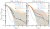Fig. 13. Comparison of the simulated and observed stacked (radial) surface brightness profiles of the [C II] emission. The left and right panels show, respectively, the stacked surface density profiles for the low-SFR (SFR < 25 M⊙ yr−1) and high-SFR (SFR ≥ 25 M⊙ yr−1) samples as defined by Ginolfi et al. (2020) based on galaxies from the ALPINE survey at z = 4.5 − 5.9. The solid lines represent the stacked profiles of (central) galaxies from the simulation at z = 5 (in blue) and z = 4 (in orange). The shaded areas represent the full range spanned by the individual profiles, which were constructed from the 2D projection of a 50 kpc cube centred on the galaxy along three orthogonal lines of sight. All profiles were smoothed with a 2D Gaussian beam of FWHM 0.9″ (as in Ginolfi et al. 2020) and normalised by the peak value of the stack. For reference, the unsmoothed stacked profiles are shown in lighter shades. The observed profiles from Ginolfi et al. (2020) are shown in black squares and red plusses for their low- and high-SFR samples, respectively.

8.2. Extent of [C II] emission in individual objects

Next we quantified the extent of the [C II] emission relative to the SF activity in our simulated galaxies. For this analysis, we included all galaxies that meet the following criteria: (i) M_* ≥ 10^8.5 M_⊙ and (ii) SFR ≥ 3 M_⊙ yr⁻¹. These were chosen to match the range of M_* and SFR values in ALPINE galaxies (Le Fèvre et al. 2020). For each galaxy in our sample, we took a sphere of radius 25 kpc centred on the galaxy and obtain projections of the same along three orthogonal lines of sights (we take these to be the coordinate axes of the simulation box) to obtain the [C II] surface brightness and SFR surface density maps. Then we computed the (cumulative) radial surface brightness profiles for each projection, from which we derived the radius enclosing 70% and 90% of the total [C II] emission – these are denoted as $r_{70,[\mathrm{C}\mathrm{I}\mathrm{I}]}$ and $r_{90,[\mathrm{C}\mathrm{I}\mathrm{I}]}$, respectively. Similarly, from the (cumulative) SFR surface density profile, we derived r_90,  SFR (as in Sect. 6, we use the SFR averaged over the last 200 Myr). For each galaxy, we also computed the cumulative [C II] luminosity profile from the full 3D distribution of [C II] within the region.

Based on these, we calculated the following parameters for each galaxy for the three orthogonal projections. As an example, we show in Fig. 14, cumulative profiles for a simulated galaxy and how these are used for calculating the three parameters and to ease their interpretation.

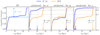Fig. 14. Example illustrating the calculation of the 𝒮, ℛ, and ℰ parameters in a simulated galaxy. The left panel shows the cumulative profile for the 3D distribution of [C II], with the dashed line marks the contribution of the central galaxy to the total [C II] emission (as evident from the flattening of the cumulative profile). The remaining fraction (denoted by 𝒮) represents the contribution of satellites. The other panels show cumulative profile constructed from the [C II] surface brightness (blue) and SFR surface density (orange). For the profiles obtained from projections, the value of the ℛ and ℰ parameters are indicated in each panel. In all but the leftmost panel, the dotted, dashed and solid horizontal lines denote cumulative fractions of 70%, 90%, and 100%, respectively. The small and large blue arrows mark $r_{70,[\mathrm{C}\mathrm{I}\mathrm{I}]}$ and $r_{90,[\mathrm{C}\mathrm{I}\mathrm{I}]}$, respectively and the orange arrow denotes r90,  SFR. The parameter $\mathcal{R}\equiv r_{90,[\mathrm{C}\mathrm{I}\mathrm{I}]}/r_{90,\mathrm{SFR}}$ is calculated from the ratio of the r values denoted by the large blue and orange arrows, while the parameter $\mathcal{E}\equiv r_{90,[\mathrm{C}\mathrm{I}\mathrm{I}]}/r_{70,[\mathrm{C}\mathrm{I}\mathrm{I}]}$ from the ratio of the large and small blue arrows.

1. The multicomponent extent parameter $\mathcal{E}\equiv r_{90,[\mathrm{C}\mathrm{I}\mathrm{I}]}/r_{70,[\mathrm{C}\mathrm{I}\mathrm{I}]}$ that measures the spread in the [C II] emission. A higher ℰ indicates a relatively large extent of the diffuse [C II] component. This would occur in galaxies where 70% of the emission is relatively confined, while the remaining 10 − 30% is more spread out, likely due to the presence of satellite galaxies. Thus, a higher ℰ denotes more extended emission relative to the bulk of the emission.

2. The parameter $\mathcal{R}\equiv r_{90,[\mathrm{C}\mathrm{I}\mathrm{I}]}/r_{90,\mathrm{SFR}}$ that quantifies the relative extent of the [C II] emission compared to SF. In this analysis, we were particularly interested in galaxies where the [C II] emission is at least twice as extended as the SF activity (i.e., ℛ ≥ 2).

3. The parameter 𝒮 that quantifies the fraction of the total [C II] emission that arises from outside the central galaxy and represents the contribution from satellites. Unlike ℛ and ℰ, this parameter is computed from the true 3D distribution of [C II] emission and is therefore agnostic to the projection axis by construction.

Note that all three parameters are agnostic to whether the [C II] emission at a given location arises from a C⁺ ion formed in situ or transported there, for example, via outflows/inflows.

From Fig. 14, it is evident that the parameters ℛ and ℰ are sensitive to the orientation of the galaxy. For instance, the y-projection of the galaxy has ℛ ∼ 1, indicating equal extent of the [C II] emission and SFR. In contrast, in the x- and z-projections, the SFR profile is more extended than the [C II] profile, resulting in ℛ < 1. Note that in this case, the ℰ value is relatively high, meaning that $r_{70,[\mathrm{C}\mathrm{I}\mathrm{I}]}$ and $r_{90,[\mathrm{C}\mathrm{I}\mathrm{I}]}$ are well separated, but owing to a more extended SFR profile, the ℛ value is low.

To better understand how the three parameters are correlated, we show in Fig. 15, how ℛ varies with ℰ and 𝒮 for our galaxy sample at z = 4. Each scatter point represents one of the orthogonal projections of a galaxy and is colour-coded by value of the third parameter. Firstly, in panel (a), we see that the parameter ℛ increases in general with ℰ. However, some galaxies⁴ with ℛ ≳ 2 exhibit a low ℰ (≲ 2). In contrast, in panel (b), we see that all galaxies with a high ℛ generally have a high 𝒮 as well, although the reverse is not always true – some galaxies have a high 𝒮 but ℛ ∼ 1. In these galaxies, satellites contribute similarly to the [C II] emission and the SF, driving the r₉₀ of both quantities to high values, and thereby reducing the ℛ (the y-projection in Fig. 14 is an example of this).

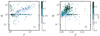Fig. 15. Distribution of our galaxies at redshift z = 4 in the ℛ-ℰ (left), ℛ-𝒮 (right) planes. The scatter points are colour-coded by the parameter 𝒮 in the left panel and by the log of parameter ℰ in the right panel. The dashed grey lines in the right panel indicates the threshold value of 𝒮 used to separate galaxies into low and high 𝒮.

In Fig. 16, we compare the extent of the r₉₀ values of the [C II] emission and the SFR. The galaxies are colour-coded according to their ℰ parameter while the shape of the symbol represents the value of the 𝒮 parameter: we split the galaxies into ‘low 𝒮’ (𝒮 < 0.1) and ‘high 𝒮’ (𝒮 ≥ 0.1) subsamples. The threshold of 0.1 or 10% was inspired by Springel et al. (2008), who found that ≈11% of the mass fraction in virialised halos is present in substructures. For reference, we also show the r₉₀ values for [C II] and SFR from observations of individual galaxies: to obtain these, we used the half-light radii r_e for the [C II] emission and UV continuum emission, reported in the respective observations. In all observations shown in Fig. 16, $r_{\mathrm{e},[\mathrm{C}\mathrm{I}\mathrm{I}]}$ and r_e,  UV are obtained from fitting exponential disk-profiles to the [C II] emission and UV continuum emission, respectively. We scaled these r_e values by 2.318 to obtain the respective r₉₀ values⁵. Since the bulk of the UV emission from galaxies arises from stars younger than ≈100 Myr (Kennicutt & Evans 2012), we further assumed that the r_90,  SFR in the observed galaxies can be approximated by the r_90, UV values. A possible caveat is that the UV sizes might be larger than the corresponding SFR sizes (e.g., see Szomoru et al. 2013, for a comparison of the half-light and half-mass radii of 0.5 < z < 2 galaxies.).

From Fig. 16, we see that the [C II] emission in many of our simulated galaxies has a similar extent as the observed galaxies at 4.5 ≲ z ≲ 5.9 from Fujimoto et al. (2020), Herrera-Camus et al. (2021), and Lambert et al. (2023). However, our simulated galaxies occupy a larger area of the parameter space compared to observations. Our galaxies where the [C II] emission is at least twice as extended as the SF activity (i.e., above the top grey dashed line, ℛ ≥ 2) exhibit preferentially higher ℰ values (darker colours of the symbol) and a higher contribution from satellites, compared to galaxies lying along the diagonal (i.e. ℛ ∼ 1 ). This is also evident from the higher median of the ℰ and 𝒮 parameters for the galaxies with ℛ ≥ 2 (see Table 7).

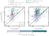Fig. 16. Comparison of $r_{90,[\mathrm{C}\mathrm{I}\mathrm{I}]}$ and r90,  SFR for simulated galaxies at redshifts z = 5 (left) and 4 (right). The galaxies are colour-coded by their multicomponent extent parameter ℰ defined as the ratio of the r90 and r70 values of the [C II] surface brightness profile. The shape of the symbol reflects the 𝒮 parameter that quantifies the satellite contribution to the total [C II] emission (see text for details). We use ‘low 𝒮’ and ‘high 𝒮’, respectively to denote galaxies with < 10% and ≥10% satellite contribution. The $r_{90,[\mathrm{C}\mathrm{I}\mathrm{I}]}$ versus r90,  SFR values of observed galaxies are shown as red open circles (Fujimoto et al. 2020), a yellow plus (Lambert et al. 2023), a green pentagon (Herrera-Camus et al. 2021), and a blue diamond (Posses et al. 2024). The black dashed line indicates a 1:1 relation, while the top and bottom grey dashed lines indicate 2:1 and 1:2 relations, respectively. Note that the error bars are not shown for Fujimoto et al. (2020) galaxies for the sake of clarity.

To summarize, we find that the inferred detection of an extended [C II] emission in a given galaxy is sensitive to the orientation of the galaxy. Nevertheless, some statistical differences emerge between galaxies with extended [C II] emission compared to their SF activity (i.e., with $\mathcal{R}\equiv r_{90,[\mathrm{C}\mathrm{I}\mathrm{I}]}/r_{90,\mathrm{SFR}}\ge 2$) and those without (i.e., ℛ < 2). Galaxies with ℛ ≥ 2 tend to have a higher contribution from satellites. They also exhibit higher ℰ values compared to the latter, indicating that while the bulk (∼70%) of the [C II] emission is relatively concentrated, the remaining fraction can extend out to 4–5 times larger radii. Overall, about 10% of our simulated galaxies at z = 4 have ℛ ≥ 2 that is, their [C II] emission extends ≥2 times farther than the SF activity; this fraction increases to 20% at z = 5. This is in agreement with recent observations pointing out the increased prevalence of extended [C II] emission towards higher redshifts (Carniani et al. 2018; Fujimoto et al. 2019; Ginolfi et al. 2020; Fudamoto et al. 2022).

9. Summary

Based on a sample of simulated galaxies with molecular cloud chemistry evolved on the fly and [C II] 158 μm line emission calculated in post-processing, we have investigated the reliability of this line as a tracer of the SF activity and molecular gas content in galaxies at redshifts 3 ≤ z ≤ 7. Here we briefly summarize our findings:

1. Redshift evolution of the [C II] luminosity function: Our simulations predict a strong time evolution in the number density of [C II] emitters, especially at the bright end. The number density of $L_{[\mathrm{C}\mathrm{I}\mathrm{I}]}\sim {10}^9{\mathrm{L}}_{\odot }$ galaxies increases by 600 times in the above redshift range. At all redshifts, a double power-law provides a better fit to our simulated LFs (Table 2).

2. Redshift evolution of the [C II]–SFR relation: The slope of the L_[C II]−SFR relation shows little evolution in the redshift range 3 ≤ z ≤ 7 while the intercept increases by ≈0.5 dex in this interval, indicating that the [C II] luminosity at given SFR increase roughly by a factor of three from z = 7 to z = 3. Notably, the scatter in the relation increases towards higher redshifts (Table 3).

3. The conversion factor α_[C II]: The conversion factor α_[C II] between the [C II] luminosity and the molecular gas mass in our simulated galaxies ranges from $\sim 1-200{\mathrm{M}}_{\odot }{\mathrm{L}}_{\odot }^{-1}$ and does not show a systematic dependence on metallicity in agreement with the findings from Zanella et al. (2018) based on a compilation of galaxies from z = 0 − 5.5. Across redshifts, α_[C II] shows a strong correlation with the SFR averaged over 5 Myr and with the SFR change diagnostic R_{5 − 200} = SFR₅/SFR₂₀₀ (Fig. 11).

4. Secondary dependences in the L_[C II]−M_mol relation: We performed a principal component analysis to quantify secondary dependences in the [C II]–M_mol relation and found a strong dependence on the SFR₅ (the star formation rate measured on a 5 Myr timescale) that evolves with redshift and a weak dependence on metallicity across redshifts (Table 5). The resulting 3-variable PCA relation predicts the true molecular gas within a factor of 1.7 (2.5) at z = 3 (z = 7). When accounting for typical observational uncertainties on L_[C II], SFR, and gas metallicity, the PCA-based relation predicts the true molecular gas mass within a factor of ∼2.5 at 3 ≤ z ≤ 5.

5. What does the [C II] emission really trace?: We investigated the correlation of L_[C II] with several galaxy-integrated properties, namely the SFR, the molecular gas mass, the total gas mass, and the metal mass in gas phase (M_metal). Among these, the [C II] emission in our simulated galaxies shows the tightest correlation with M_metal across redshifts (Tables 3 and 6).

6. Extended [C II] emission: We observed that our stacked [C II] surface brightness profiles show a similar extent as the low-SFR galaxy sample from Ginolfi et al. (2020), although some individual galaxies also exhibit a similar extent as their high-SFR sample. We further found that galaxies where the [C II] emission extends twice or more farther than the SF activity preferentially exhibit a spatial distribution wherein the bulk (≳70%) of the [C II] emission is confined to the central galaxy, while the remaining ≲30% extends out to larger distances because of the presence of satellites. The typical fractional contribution of satellites to the total [C II] emission in these galaxies is ≈5 − 7 times higher than that in galaxies without extended emission (see Table 7).

Acknowledgments

The authors thank an anonymous reviewer for their valuable feedback that helped improved this manuscript. We thank R. Teyssier for making the RAMSES code publicly available. They gratefully acknowledge the Collaborative Research Center 1601 (SFB 1601 sub-project C5) funded by the Deutsche Forschungsgemeinschaft (DFG, German Research Foundation) – 500700252. Early stages of this work were carried out within the Collaborative Research Centre 956 (SFB 956 sub-project C4), funded by the DFG – 184018867. The authors acknowledge the Gauss Centre for Supercomputing e.V. (https://www.gauss-centre.eu/) for funding this project by providing computing time on the GCS Supercomputer SuperMUC-NG at the Leibniz Supercomputing Centre (http://www.lrz.de). They are thankful to the Max Planck Society (MPG) for providing computing time on the supercomputer Raven at the Max Planck Computing and Data Facility (https://www.mpcdf.mpg.de), where part of the MARIGOLD simulations were performed. PK is a part of the International Max Planck Research School in Astronomy and Astrophysics, the Bonn Cologne Graduate School, and a guest at the Max Planck Institute for Radio Astronomy in Bonn.

References

Appendix A: Modelling [C II] emission

For a two-level system such as the C⁺ fine-structure transition, the excitation temperature (T_ex) captures the relative population in the upper (u) and lower (l) energy levels of the transition:

$$\begin{array}{c}\hfill \frac{n_u}{n_l}=\frac{g_u}{g_l}{e}^{-T_{\ast }/T_{\mathrm{ex}}}.\end{array}$$(A.1)

Here g_u and g_l are the statistical weights of the upper and lower levels with an energy difference of k_BT_* (k_B being the Boltzmann constant), and n_u + n_l = n_C⁺. In statistical equilibrium, level populations are determined by the balance between excitation and deexcitation processes:

$$\begin{array}{c}\hfill n_l(B_{\mathit{lu}}U+C_{\mathit{lu}})=n_u(A_{\mathit{ul}}+B_{\mathit{ul}}U+C_{\mathit{ul}}),\end{array}$$(A.2)

where U is the energy density at the transition frequency ν; A_ul, B_ul and B_lu are the Einstein coefficients for spontaneous decay, stimulated decay, and stimulated excitation, respectively, C_ul and C_lu are the collision deexcitation and excitation rates and, in the case of multiple collision partners, can be obtained from the respective collision rate coefficients and number densities as:

$$\begin{array}{c}\hfill C_{\mathit{ul}}={\displaystyle \sum _{i=1}^N}{R}_{ul,i}{n}_i.\end{array}$$(A.3)

The upward and downward collision rate coefficients are related as:

$$\begin{array}{c}\hfill R_{\mathit{lu}}=R_{\mathit{ul}}\frac{g_u}{g_l}{e}^{-T_{\ast }/T_{\mathrm{kin}}},\end{array}$$(A.4)

where T_kin is the kinetic temperature related to the thermal motions of the collision partner. The collision rate coefficients are taken from Goldsmith et al. (2012):

$$\begin{array}{cc}\hfill R_{\mathit{ul}}(e^{-})& =8.7\times {10}^{-8}{(T_e/2000)}^{-0.37}{\mathrm{cm}}^3{s}^{-1};\hfill \end{array}$$(A.5)

$$\begin{array}{cc}\hfill R_{\mathit{ul}}(\mathrm{H})& =7.6\times {10}^{-10}{(T_{\mathrm{kin}}/100)}^{0.14}{\mathrm{cm}}^3{s}^{-1};\hfill \end{array}$$(A.6)

$$\begin{array}{cc}\hfill R_{\mathit{ul}}({\mathrm{H}}_2\left\}\right\})& =3.8\times {10}^{-10}{(T_{\mathrm{kin}}/100)}^{0.14}{\mathrm{cm}}^3{s}^{-1},\hfill \end{array}$$(A.7)

where T_e is the electron temperature. In the following, we assume T_e = T_kin. We obtain the kinetic temperature at each sub-grid density using the temperature density relation (from Hu et al. 2021) and is identical to the one adopted in HYACINTH (see Khatri et al. 2024, for details). The C⁺ and H₂ number densities are obtained directly from the simulations. To obtain the number density of atomic hydrogen ($\mathrm{H}$), we assume that gas at densities $n_{\mathrm{H},\mathrm{tot}}\gtrsim 0.013{\mathrm{cm}}^{-3}$ is well-shielded and n_H⁺ = 0 (Tajiri & Umemura 1998); below these densities, we assume all hydrogen to be ionised, that is, n_H⁺ = n_H, tot. The electron number density follows from charge conservation that is, n_e⁻ = n_C⁺ + n_H⁺. Note that, similar to Gong et al. (2012) and Vallini et al. (2015), we do not consider the pumping effect from the soft UV background from stars at 1330 Å.

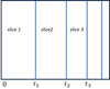Fig. A.1. Schematic representation of the plane-parallel slices in a grid cell.

Now, suppose that a given grid cell of sidelength L can be split into N plane-parallel slices as shown in Fig. A.1. In the following, we take N = 3 for simplicity, but in practice, use 20 slices in each slice, which were sufficient to reach convergence. The width and density of each slice are determined by the sub-grid density PDF (same as in HYACINTH) within the cell. If T_ex, i is the excitation temperature in slice i, then the energy density generated in the slice at the transition frequency ν can then be written as

$$\begin{array}{c}\hfill U_{\nu }(T_{\mathrm{ex},i})=\frac{4\pi }{c}{B}_{\nu }(T_{\mathrm{ex},i})=\frac{8\pi h{\nu }^3}{c^3}\frac{1}{exp(h\nu /k_{\mathrm{B}}{T}_{\mathrm{ex},i})-1}.\end{array}$$(A.8)

Assuming the entire region is permeated by a background like the CMB at temperature T_bg with energy density U_ν(T_bg), the total energy density in a slice will have three contributions:

1. the energy density generated in the slice weighted by the fraction of the energy that does not escape the slice (self-absorption, denoted by κ_ii);

2. the energy density from all other slices where the energy density of the emitting slice i is weighted by the fraction that is absorbed by the absorbing slice j (denoted by κ_ij);

3. the energy density from the background (CMB in this case).

Following Goldsmith et al. (2012), the total energy density in the slice at the [C II] frequency can be written as:

$$\begin{array}{cc}\hfill U_1& =(1-{\kappa }_{11})U_{\nu }(T_{\mathrm{bg}})+{\kappa }_{11}{U}_{\nu }(T_{\mathrm{ex},1})\hfill \\ \hfill & +{\kappa }_{21}{U}_{\nu }(T_{\mathrm{ex},2})+{\kappa }_{31}{U}_{\nu }(T_{\mathrm{ex},3}).\hfill \end{array}$$(A.9)

Similarly,

$$\begin{array}{cc}\hfill U_2& =(1-{\kappa }_{22})U_{\nu }(T_{\mathrm{bg}})+{\kappa }_{12}{U}_{\nu }(T_{\mathrm{ex},1})\hfill \\ \hfill & +{\kappa }_{22}{U}_{\nu }(T_{\mathrm{ex},2})+{\kappa }_{32}{U}_{\nu }(T_{\mathrm{ex},3});\hfill \end{array}$$(A.10)

and

$$\begin{array}{cc}\hfill U_3& =(1-{\kappa }_{33})U_{\nu }(T_{\mathrm{bg}})+{\kappa }_{13}{U}_{\nu }(T_{\mathrm{ex},1})\hfill \\ \hfill & +{\kappa }_{23}{U}_{\nu }(T_{\mathrm{ex},2})+{\kappa }_{33}{U}_{\nu }(T_{\mathrm{ex},3}).\hfill \end{array}$$(A.11)

If U₁, U₂, U₃ are known, they can be used to evaluate the level population in each slice by balancing the upward and downward transitions as (e.g., for slice 1):

$$\begin{array}{c}\hfill n_{u,1}(A_{\mathit{ul}}+B_{\mathit{ul}}{U}_1+C_{\mathit{ul}})=n_{l,1}(B_{\mathit{lu}}{U}_1+C_{\mathit{lu}}),\end{array}$$(A.12)

and the excitation temperature T_ex, 1 can be obtained using Eq. (A.1). Following Goldsmith et al. (2012), the optical depth for slice 1 can be calculated from the excitation temperature T_ex, 1 as:

$$\begin{array}{c}\hfill \begin{array}{cc}\hfill {\tau }_1& =\frac{h{B}_{\mathit{lu}}N({\mathrm{C}}^{+})}{\delta v}\frac{1-e^{-h\nu /k_{\mathrm{B}}{T}_{\mathrm{ex},1}}}{1+(g_u/g_l)e^{-h\nu /k_{\mathrm{B}}{T}_{\mathrm{ex},1}}}\hfill \\ \hfill & =\frac{g_u}{g_l}\frac{A_{\mathit{ul}}{\lambda }_{\mathit{ul}}^{3}N({\mathrm{C}}^{+})}{8\pi \sqrt{8ln(2)}{\sigma }_v}\frac{1-e^{-h\nu /k_{\mathrm{B}}{T}_{\mathrm{ex},1}}}{1+(g_u/g_l)e^{-h\nu /k_{\mathrm{B}}{T}_{\mathrm{ex},1}}},\hfill \end{array}\end{array}$$(A.13)

where λ_ul is the wavelength of the [C II] line and N(C⁺) denotes the column density of C⁺ from the edge of the cell to the slice i. The above expression approximates the line profile function ϕ_ν at line centre by δv⁻¹. where δv is the line width (${\delta }_v=\sqrt{8ln2}{\sigma }_v$ for a Gaussian velocity distribution with 1-D velocity dispersion σ_v). We obtain the 1-D velocity dispersion σ_v for the cells in our simulations following the approach of Olsen et al. (2015): the velocity dispersion in a giant molecular cloud (GMC) of mass M_GMC and radius R_GMC is given as

$$\begin{array}{c}\hfill {\sigma }_v=1.2\mathrm{km}{\mathrm{s}}^{-1}{\left(\frac{R_{\mathrm{GMC}}}{\mathrm{pc}}\right)}^{-1/2}{\left(\frac{M_{\mathrm{GMC}}}{290{\mathrm{M}}_{\odot }}\right)}^{1/2},\end{array}$$(A.14)

where we approximate $R_{\mathrm{GMC}}\approx \frac{1}{2}\mathrm{\Delta }L$ and M_GMC = M_{gas,  cell}.

The system of equations (A.1), (A.9)-(A.13) can be solved iteratively. We start with the optically thin case where all emitted radiation freely escapes (i.e., κ_ij = 0   ∀ {i, j}), and obtain an initial estimate of n_u, i using Eq. (A.12). These estimates are then used to obtain a first estimate of T_ex, 1, T_ex, 2, T_ex, 3 using Eq. (A.1). These determine the optical depths τ₁, τ₂, τ₃ using Eq. (A.13). Using these, the κ values can be updated and the entire procedure is repeated until convergence⁶.

Once we have a set of self-consistent T_ex and κ values, we can calculate the emissivity of each slice. Following Goldsmith et al. (2012), the emissivity in slice 1 can be written as

$$\begin{array}{c}\hfill {ϵ}_1=n_{u,1}{A}_{\mathit{ul}}{\gamma }_{1}h\nu [1-\frac{e^{(h\nu /k_{\mathrm{B}}{T}_{\mathrm{ex},1})}-1}{e^{(h\nu /k_{\mathrm{B}}{T}_{\mathrm{bg}})}-1}],\end{array}$$(A.15)

where

$$\begin{array}{c}\hfill {\gamma }_i=1.0-{\displaystyle \sum _{j=1}^3}{\kappa }_{\mathit{ij}}\end{array}$$(A.16)

denotes the final escape fraction for slice i, that is the fraction of photons emitted in slice i that manage to escape the cell and accounts for absorption from all intervening slices.

The total luminosity from the cell can be written as:

$$\begin{array}{c}\hfill L_{[\mathrm{C}\mathrm{I}\mathrm{I}]}={\displaystyle \sum _{i=1}^N}{\gamma }_i{ϵ}_i\mathrm{\Delta }{V}_i,\end{array}$$(A.17)

where ΔV_i = 𝒫_V(n_i) Δn_i V_cell is the volume of each slice, and N is the number of slices in the cell. The galaxy luminosity is obtained by summing over the [C II] emission from all cells within the galaxy. We note that our method assumes that the [C II] emission from the different grid cells are radiatively decoupled and the total [C II] emission from a galaxy is the sum of the emission from each cell.

Appendix B: Model validation

We validate our [C II] emission model by comparing its output with the photoionisation code CLOUDY (version 17.02; Ferland et al. 1992). To do this, we compute the luminosity emerging from a plane-parallel slab with a side length of $\mathrm{\Delta }x=38\mathrm{pc}$, corresponding to the minimum spatial resolution achieved in our M25 run at z = 4. The CMB is included for z = 4.

To span the range of gas densities and metallicities exhibited by PDRs and molecular clouds, we compute the luminosity for a 2D grid with hydrogen number density $n_{\mathrm{H}}\in [{10}^0,{10}^4]{\mathrm{cm}}^{-3}$ and gas metallicity $Z_{\mathrm{gas}}\in [{10}^{-1.8},{10}^0]{\mathrm{Z}}_{\odot }$. The slabs have a uniform density, metallicity and temperature. We assume that the kinetic temperature is uniform throughout the slab. For each set of (n_H,  Z_gas) values, we obtain the temperature using the metallicity-dependent temperature density relation from Hu et al. (2021, same as in HYACINTH). We assume that the elemental abundance of carbon f_C, tot scales as $f_{\mathrm{C},\mathrm{tot}}=2.9\times {10}^{-4}{Z}_{\mathrm{gas}}/{\mathrm{Z}}_{\odot }$ (Asplund et al. 2009). For each of these models, CLOUDY computes the abundances of different chemical species as a function of the depth into the slab. The C⁺, H₂, and H I abundances are used as inputs to our model compute the emergent luminosity from the model cells. We further assume n_e⁻ = n_C⁺.

The results of the comparison are shown in Fig. B.1. In the following, we denote the [C II] luminosity predicted by our model as L and the one from CLOUDY as $L_{\mathrm{C}\mathrm{L}\mathrm{O}\mathrm{U}\mathrm{D}\mathrm{Y}}$. At all values of T_kin, the distribution of L is very similar to $L_{\mathrm{C}\mathrm{L}\mathrm{O}\mathrm{U}\mathrm{D}\mathrm{Y}}$, with L from both approaches increasing with density at a fixed metallicity. Conversely, at fixed densities $n_{\mathrm{H}}\lesssim {10}^3{\mathrm{cm}}^{-3}$, L increases with metallicity and the variation with metallicity is minimal at higher densities. At $\log (Z_{\mathrm{gas}}/{\mathrm{Z}}_{\odot })\gtrsim {10}^{-0.6}$ (i.e., $Z_{\mathrm{gas}}\gtrsim 0.25{\mathrm{Z}}_{\odot }$), our model overpredicts L_[C II] at low densities ($n_{\mathrm{H}}\lesssim {10}^2{\mathrm{cm}}^{-3}$) and underpredicts at intermediate densities (${10}^2{\mathrm{cm}}^{-3}\lesssim {\mathrm{n}}_{\mathrm{H}}\lesssim {10}^3{\mathrm{cm}}^{-3}$). Across the parameter space explored here, we find that the deviation between our model and CLOUDY can be as high as ±50%. However, in most ( 33/49 grid points in the right panel of Fig. B.1) of the parameter space there is a ≤30% deviation between the L_[C II] from the two approaches, particularly at high densities ($n_{\mathrm{H}}\gtrsim {10}^3{\mathrm{cm}}^{-3}$). We note that a deviation of ≲30 − 50% is much lower than the typical systematic uncertainties associated with observational measurements of the [C II] luminosity in high-redshift galaxies (see for example, Béthermin et al. 2020; Schaerer et al. 2020, for the ALPINE survey) that typically have errors/uncertainties up to a factor of 2, implying that a difference of 30-50% is much lower than the expected observational uncertainties.

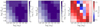Fig. B.1. Tests of [C II] emission model with CLOUDY. The left and middle panels show, respectively, the luminosity from our model and CLOUDY, while the right panel shows the ratio of the two. For each set of (nH,  Zgas) values, the temperature is obtained using the temperature-density relation from Hu et al. (2021).

Appendix C: Fit to the simulated luminosity function

Fig. C.1 shows a comparison between the Schechter function and double power-law fits to the predicted [C II] LFs from our simulations at 3 ≤ z ≤ 7.

In Fig. C.2, we show the covariance distributions obtained from the Markov Chain Monte Carlo (MCMC) fitting of our predicted [C II] luminosity function at z = 4 with a DPL given in Eq. 2. The fitting was performed using the python package emcee and includes two parameters – ΔM25 and ΔM50 that represent variation of the log ϕ of the two simulation volumes from the cosmic log ϕ*, because of sample variance. We see that the posterior distributions of the all parameters are well-behaved and smooth, and that the three parameters are highly correlated. We obtain similar results at other redshifts.

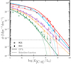Fig. C.1. Comparison of the Schechter function (dotted lines) and DPL (solid lines) fits to our simulated LFs from the two simulations at different redshifts (from top to bottom, z increases from 3 to 7). The open squares and diamonds represent the separate LFs from the simulations that are used to obtain the fit parameters using an MCMC analysis. The error bars represent the 16 CL upper and lower Poisson uncertainties on number counts (Gehrels 1986). The dashed and dotted horizontal lines represent a number count of 1 per dex in the entire simulation volume of M25 and M50, respectively.

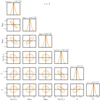Fig. C.2. Covariance distributions and PDFs of the double power-law function (Eq. 2) parameters: ϕ*, L*, α, β, and two additional parameters: ΔM25 and ΔM50, from MCMC runs using the python package emcee for simulated LF at z = 3.

Appendix D: Surface densities

In Fig. D.1, we show a scatter plot of the surface densities of CO and C⁺ as a function of the SFR (left), gas (middle), and metal (right) surface density. In all panels, we find that while Σ_CO continues to increase at high surface densities, Σ_C⁺ shows a plateau. This results in a decrease in the slope of the $\log {\mathrm{\Sigma }}_{[\mathrm{C}\mathrm{I}\mathrm{I}]}$ versus log Σ_SFR curve at high Σ_SFR.

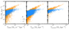Fig. D.1. The surface density of CO and C+ as a function of the SFR surface density (left), the total gas surface density (middle), and the total metal surface density (right), for galaxies used in Fig. 8.

All Tables

All Figures

	Fig. 1. Face-on view of a simulated galaxy at z = 4. From left to right, the columns show the surface density of young stars (with ages ≤ 200 Myr), total gas (including H2) surface density, H2 surface density, and [C II] surface brightness. In each panel, the circle indicates 0.1 times the virial radius of the parent DM halo.
In the text

Fig. 2. Conditional [C II] LF from the M25 (dashed lines) and M50 (solid lines) simulations at redshifts z = 5 and 3 for central galaxies (left panels), satellites galaxies (middle panels), and all galaxies (right panels). The coloured lines show the CLF of emitters residing in DM halos in different Mhalo bins and the black lines show the total LFs. The dotted grey line in the right panels denotes the luminosity threshold, Lthr, below which the total LFs from two simulations differ significantly due to resolution effects.

In the text

Fig. 3. Simulated [C II] LF compared with observational estimates. The coloured lines represent the best-fit DPL – Eq. (2) – to the simulated LF and the shaded area represents the central 68% credibility range obtained using the MCMC chains. Black stars represent the observational estimates at z ∼ 4.5 from the ALPINE survey (Yan et al. 2020) and the grey arrow shows the lower limit from Swinbank et al. (2012) based on observations of two galaxies at z ∼ 4.4. The dashed and dotted horizontal lines represent a number count of 1 per dex in the entire simulation volume of M25 and M50, respectively. The [C II] LF from Popping et al. (2016) and Lagache et al. (2018) both based on a semi-analytical galaxy formation model, and from Garcia et al. (2024) obtained by post-processing the SIMBA simulations at z = 6 and 5 are included in the respective panels.

In the text

Fig. 4. Comparison of the cosmic [C II] luminosity density (ρ[C II]) for different luminosity cuts in the MARIGOLD simulations with observational estimates from ALPINE (Loiacono et al. 2021) – clustered and field estimates in pink and blue, respectively; from REBELS (Aravena et al. 2024) in purple and from a semi-empirical model by Roy & Lapi (2025) shown as an orange dashed line. The ρ[C II] from the simulations is obtained by integrating the LFs shown in Fig. 3 down to log(Lmin/L⊙) = 5 (black), 7 (red), and 7.5 (blue). The shaded regions represent the 16–84 percentile range of ρ[C II] obtained from the LFs.

In the text

	Fig. 5. Distribution of the MARIGOLD galaxies in the SFR-Mmol plane at different redshifts. These are shown as purple hexbins, where the counts are sampled logarithmically.
In the text

Fig. 6. SFR versus M* in the MARIGOLD galaxies at different redshifts compared with observational estimates of the main-sequence (MS) of star-forming galaxies. These include the MS relations from Schreiber et al. (2015, black) and Popesso et al. (2023, red) at the respective redshifts, and the MS relations from Clarke et al. (2024, orange) based on a sample of galaxies at 2.7 ≤ z ≤ 4 and Khusanova et al. (2021, blue) based on ALPINE galaxies. The coloured errors bars on the left-hand side denote the scatter of the respective MS relations. All observed relations are extrapolated beyond the range constrained by the respective studies using a dashed line of the same colour.

In the text

Fig. 7. $[\mathrm{C}\mathrm{I}\mathrm{I}]-\mathrm{SFR}$ relation from the MARIGOLD simulations at 3 ≤ z ≤ 7 compared with observations. The simulated galaxy population is represented as purple hexbins, with the colour indicating the galaxy counts per bin. The red line showing the best-fit to these galaxies (see Table 3 for the fit parameters). In each panel, we report the Spearman’s rank correlation coefficient (ρ) and the 1σ scatter around the best-fit relation. The best-fit relation from De Looze et al. (2014) for their high−z (0.5 < z < 6.6) sample is shown in orange, with the shaded area representing the 1σ scatter. The blue line indicates the best-fit relation for 4.5 ≲ z ≲ 5.9 galaxies from the ALPINE survey (Schaerer et al. 2020). The best-fits mentioned above are extrapolated beyond the range constrained by the respective studies using a dashed line of the same colour. The individual ALPINE galaxies (at 4.5 ≲ z ≲ 5.9), the literature sample (at 5 ≲ z ≲ 7.6) taken from Olsen et al. (2015), and REBELS-25 from the REBELS survey Rowland et al. (2024) are shown with blue, pink, and black symbols, respectively. The relations from other simulations are shown as dotted lines. The relations from Lagache et al. (2018) at the respective redshift are shown in grey. The olive and cyan dotted lines along with the scatter represent the Vallini et al. (2015) relations with N = 1 and N = 3, respectively for the Kennicutt–Schmidt relation. In both cases we show the relation assuming the median Zgas of our simulated galaxies at a given redshift. The pink and teal lines represent the relations from Leung et al. (2020) and Vizgan et al. (2022), respectively, both obtained by post-processing the z ∼ 6 snapshot of the SIMBA simulations (Davé et al. 2020) with different versions of SíGAME (Olsen et al. 2015, 2017). The grey line represents the relation from Casavecchia et al. (2024).

In the text

Fig. 8. Spatially resolved $[\mathrm{C}\mathrm{I}\mathrm{I}]-\mathrm{SFR}$ relation for the MARIGOLD galaxies at z = 4. The galaxies are divided into different stellar-mass bins (the number of galaxies in each bin is indicated in the legend). The solid lines show the median ${\mathrm{\Sigma }}_{[\mathrm{C}\mathrm{I}\mathrm{I}]}$ as a function of the SFR surface density (left), of the gas surface density (middle), and of the H2 surface density (right). The shaded areas represent the 16–84 percentile range. In the left panel, dashed lines indicate the empirical relations from De Looze et al. (2014, red) based on local dwarf galaxies from the Herschel Dwarf Galaxy Survey, for ALPINE galaxies in black (based on global values only Schaerer et al. 2020, black), and for a sample of galaxies at 5 < z < 7.2 from Carniani et al. (2018, teal). For the simulated galaxies, the [C II] surface brightness, and the SFR, gas, and H2 surface densities were obtained from a face-on projection of a cube centred on the galaxy and of side length equal to twice the radius of the galaxy.

In the text

Fig. 9. [C II]−Mmol relation from our simulations compared with observations. The simulated galaxies are represented by purple hexbins, where the colour indicates the number of galaxies in each bin. The solid red line gives the ordinary least squares linear fit to these galaxies, with the fit parameters listed in Table 3. In each panel, we report the Spearman’s rank correlation coefficient (ρ) and the 1σ scatter around the best-fit relation. The best fit to the observed galaxy sample at z = 0 − 5.5 by Zanella et al. (2018) is shown in blue and the fit to the z ∼ 0 dwarf galaxies (Madden et al. 2020) is shown in lime. The relation from SIMBA simulations at z = 6 (Vizgan et al. 2022) is shown in orange. As in Fig. 7, the extrapolated Zanella et al. (2018) relation is shown as a dashed line of the same colour.

In the text

	Fig. 10. Probability distribution function of the conversion factor α[C II] exhibited by our simulated galaxies at different redshifts.
In the text

Fig. 11. Conversion factor α[C II] in our simulated galaxies as a function of gas metallicity (panel a), the SFR averaged over the last 5 Myr (panel b), the SFR averaged over the last 200 Myr (panel c), and the SFR change diagnostic R5 − 200 (panel d, see text) at different redshifts. The coloured symbols represent the median α[C II] in each bin, while the error bars represent the 16–84 percentiles. The Spearman’s rank correlation coefficient between the variables on the y and x axes are shown in each panel as well. The grey dotted line denotes the mean α[C II] from Zanella et al. (2018) and the shaded band represents the corresponding scatter.

In the text

Fig. 12. Comparison of the predicted molecular gas mass estimates with the true molecular gas mass using two different approaches for simulated galaxies at z = 4. Panel a shows the performance of the best-fit relation between Mmol and L[C II], while panels b–d present results from different PCA-based relations (as indicated in the title of each panel). The corresponding relations are listed in Table 5. In panels a–d, the top-left corner reports σ, the standard deviation of the offset between the predicted and true Mmol (both in log scale). Panel e compares the distributions of these offsets from the different approaches.

In the text

Fig. 13. Comparison of the simulated and observed stacked (radial) surface brightness profiles of the [C II] emission. The left and right panels show, respectively, the stacked surface density profiles for the low-SFR (SFR < 25 M⊙ yr−1) and high-SFR (SFR ≥ 25 M⊙ yr−1) samples as defined by Ginolfi et al. (2020) based on galaxies from the ALPINE survey at z = 4.5 − 5.9. The solid lines represent the stacked profiles of (central) galaxies from the simulation at z = 5 (in blue) and z = 4 (in orange). The shaded areas represent the full range spanned by the individual profiles, which were constructed from the 2D projection of a 50 kpc cube centred on the galaxy along three orthogonal lines of sight. All profiles were smoothed with a 2D Gaussian beam of FWHM 0.9″ (as in Ginolfi et al. 2020) and normalised by the peak value of the stack. For reference, the unsmoothed stacked profiles are shown in lighter shades. The observed profiles from Ginolfi et al. (2020) are shown in black squares and red plusses for their low- and high-SFR samples, respectively.

In the text

Fig. 14. Example illustrating the calculation of the 𝒮, ℛ, and ℰ parameters in a simulated galaxy. The left panel shows the cumulative profile for the 3D distribution of [C II], with the dashed line marks the contribution of the central galaxy to the total [C II] emission (as evident from the flattening of the cumulative profile). The remaining fraction (denoted by 𝒮) represents the contribution of satellites. The other panels show cumulative profile constructed from the [C II] surface brightness (blue) and SFR surface density (orange). For the profiles obtained from projections, the value of the ℛ and ℰ parameters are indicated in each panel. In all but the leftmost panel, the dotted, dashed and solid horizontal lines denote cumulative fractions of 70%, 90%, and 100%, respectively. The small and large blue arrows mark $r_{70,[\mathrm{C}\mathrm{I}\mathrm{I}]}$ and $r_{90,[\mathrm{C}\mathrm{I}\mathrm{I}]}$, respectively and the orange arrow denotes r90,  SFR. The parameter $\mathcal{R}\equiv r_{90,[\mathrm{C}\mathrm{I}\mathrm{I}]}/r_{90,\mathrm{SFR}}$ is calculated from the ratio of the r values denoted by the large blue and orange arrows, while the parameter $\mathcal{E}\equiv r_{90,[\mathrm{C}\mathrm{I}\mathrm{I}]}/r_{70,[\mathrm{C}\mathrm{I}\mathrm{I}]}$ from the ratio of the large and small blue arrows.

In the text

	Fig. 15. Distribution of our galaxies at redshift z = 4 in the ℛ-ℰ (left), ℛ-𝒮 (right) planes. The scatter points are colour-coded by the parameter 𝒮 in the left panel and by the log of parameter ℰ in the right panel. The dashed grey lines in the right panel indicates the threshold value of 𝒮 used to separate galaxies into low and high 𝒮.
In the text

Fig. 16. Comparison of $r_{90,[\mathrm{C}\mathrm{I}\mathrm{I}]}$ and r90,  SFR for simulated galaxies at redshifts z = 5 (left) and 4 (right). The galaxies are colour-coded by their multicomponent extent parameter ℰ defined as the ratio of the r90 and r70 values of the [C II] surface brightness profile. The shape of the symbol reflects the 𝒮 parameter that quantifies the satellite contribution to the total [C II] emission (see text for details). We use ‘low 𝒮’ and ‘high 𝒮’, respectively to denote galaxies with < 10% and ≥10% satellite contribution. The $r_{90,[\mathrm{C}\mathrm{I}\mathrm{I}]}$ versus r90,  SFR values of observed galaxies are shown as red open circles (Fujimoto et al. 2020), a yellow plus (Lambert et al. 2023), a green pentagon (Herrera-Camus et al. 2021), and a blue diamond (Posses et al. 2024). The black dashed line indicates a 1:1 relation, while the top and bottom grey dashed lines indicate 2:1 and 1:2 relations, respectively. Note that the error bars are not shown for Fujimoto et al. (2020) galaxies for the sake of clarity.

In the text

	Fig. A.1. Schematic representation of the plane-parallel slices in a grid cell.
In the text

	Fig. B.1. Tests of [C II] emission model with CLOUDY. The left and middle panels show, respectively, the luminosity from our model and CLOUDY, while the right panel shows the ratio of the two. For each set of (nH,  Zgas) values, the temperature is obtained using the temperature-density relation from Hu et al. (2021).
In the text

Fig. C.1. Comparison of the Schechter function (dotted lines) and DPL (solid lines) fits to our simulated LFs from the two simulations at different redshifts (from top to bottom, z increases from 3 to 7). The open squares and diamonds represent the separate LFs from the simulations that are used to obtain the fit parameters using an MCMC analysis. The error bars represent the 16 CL upper and lower Poisson uncertainties on number counts (Gehrels 1986). The dashed and dotted horizontal lines represent a number count of 1 per dex in the entire simulation volume of M25 and M50, respectively.

In the text

	Fig. C.2. Covariance distributions and PDFs of the double power-law function (Eq. 2) parameters: ϕ*, L*, α, β, and two additional parameters: ΔM25 and ΔM50, from MCMC runs using the python package emcee for simulated LF at z = 3.
In the text

	Fig. D.1. The surface density of CO and C+ as a function of the SFR surface density (left), the total gas surface density (middle), and the total metal surface density (right), for galaxies used in Fig. 8.
In the text

References

- Accurso, G., Saintonge, A., Catinella, B., et al. 2017, MNRAS, 470, 4750 [NASA ADS] [Google Scholar]
- Akins, H. B., Fujimoto, S., Finlator, K., et al. 2022, ApJ, 934, 64 [NASA ADS] [CrossRef] [Google Scholar]
- Aravena, M., Heintz, K., Dessauges-Zavadsky, M., et al. 2024, A&A, 682, A24 [NASA ADS] [CrossRef] [EDP Sciences] [Google Scholar]
- Asplund, M., Grevesse, N., Sauval, A. J., & Scott, P. 2009, ARA&A, 47, 481 [NASA ADS] [CrossRef] [Google Scholar]
- Atek, H., Labbé, I., Furtak, L. J., et al. 2024, Nature, 626, 975 [NASA ADS] [CrossRef] [Google Scholar]
- Bernal, J. L., & Kovetz, E. D. 2022, A&ARv, 30, 5 [NASA ADS] [CrossRef] [Google Scholar]
- Béthermin, M., Fudamoto, Y., Ginolfi, M., et al. 2020, A&A, 643, A2 [Google Scholar]
- Bigiel, F., Leroy, A., Walter, F., et al. 2008, AJ, 136, 2846 [NASA ADS] [CrossRef] [Google Scholar]
- Bothwell, M. S., Maiolino, R., Cicone, C., Peng, Y., & Wagg, J. 2016, A&A, 595, A48 [NASA ADS] [CrossRef] [EDP Sciences] [Google Scholar]
- Bouwens, R. J., Smit, R., Schouws, S., et al. 2022, ApJ, 931, 160 [NASA ADS] [CrossRef] [Google Scholar]
- Carilli, C. L., & Walter, F. 2013, ARA&A, 51, 105 [NASA ADS] [CrossRef] [Google Scholar]
- Carniani, S., Maiolino, R., Smit, R., & Amorín, R. 2018, ApJ, 854, L7 [Google Scholar]
- Casavecchia, B., Maio, U., Péroux, C., & Ciardi, B. 2024, A&A, 689, A106 [NASA ADS] [CrossRef] [EDP Sciences] [Google Scholar]
- Casavecchia, B., Maio, U., Péroux, C., & Ciardi, B. 2025, A&A, 693, A119 [NASA ADS] [CrossRef] [EDP Sciences] [Google Scholar]
- Catán, V., González-López, J., Solimano, M., et al. 2024, A&A, 692, A215 [NASA ADS] [CrossRef] [EDP Sciences] [Google Scholar]
- Clarke, L., Shapley, A. E., Sanders, R. L., et al. 2024, ApJ, 977, 133 [NASA ADS] [CrossRef] [Google Scholar]
- Cormier, D., Abel, N. P., Hony, S., et al. 2019, A&A, 626, A23 [NASA ADS] [CrossRef] [EDP Sciences] [Google Scholar]
- Crawford, M. K., Genzel, R., Townes, C. H., & Watson, D. M. 1985, ApJ, 291, 755 [Google Scholar]
- da Cunha, E., Groves, B., Walter, F., et al. 2013, ApJ, 766, 13 [Google Scholar]
- Davé, R., Crain, R. A., Stevens, A. R. H., et al. 2020, MNRAS, 497, 146 [Google Scholar]
- De Breuck, C., Lundgren, A., Emonts, B., et al. 2022, A&A, 658, L2 [CrossRef] [EDP Sciences] [Google Scholar]
- Decarli, R., Walter, F., Gónzalez-López, J., et al. 2019, ApJ, 882, 138 [Google Scholar]
- De Looze, I., Baes, M., Bendo, G. J., Cortese, L., & Fritz, J. 2011, MNRAS, 416, 2712 [Google Scholar]
- De Looze, I., Cormier, D., Lebouteiller, V., et al. 2014, A&A, 568, A62 [NASA ADS] [CrossRef] [EDP Sciences] [Google Scholar]
- Dessauges-Zavadsky, M., Ginolfi, M., Pozzi, F., et al. 2020, A&A, 643, A5 [NASA ADS] [CrossRef] [EDP Sciences] [Google Scholar]
- D’Eugenio, C., Daddi, E., Liu, D., & Gobat, R. 2023, A&A, 678, L9 [NASA ADS] [CrossRef] [EDP Sciences] [Google Scholar]
- Díaz-Santos, T., Armus, L., Charmandaris, V., et al. 2013, ApJ, 774, 68 [Google Scholar]
- Ferland, G. J., Peterson, B. M., Horne, K., Welsh, W. F., & Nahar, S. N. 1992, ApJ, 387, 95 [NASA ADS] [CrossRef] [Google Scholar]
- Foreman-Mackey, D., Conley, A., Meierjurgen Farr, W., et al. 2013, Astrophysics Source Code Library [record ascl:1303.002] [Google Scholar]
- Fudamoto, Y., Smit, R., Bowler, R. A. A., et al. 2022, ApJ, 934, 144 [NASA ADS] [CrossRef] [Google Scholar]
- Fujimoto, S., Ouchi, M., Ferrara, A., et al. 2019, ApJ, 887, 107 [Google Scholar]
- Fujimoto, S., Silverman, J. D., Bethermin, M., et al. 2020, ApJ, 900, 1 [Google Scholar]
- Garcia, K., Narayanan, D., Popping, G., et al. 2024, ApJ, 974, 197 [NASA ADS] [CrossRef] [Google Scholar]
- Gehrels, N. 1986, ApJ, 303, 336 [Google Scholar]
- Ginolfi, M., Jones, G. C., Béthermin, M., et al. 2020, A&A, 633, A90 [NASA ADS] [CrossRef] [EDP Sciences] [Google Scholar]
- Goldsmith, P. F., Langer, W. D., Pineda, J. L., & Velusamy, T. 2012, ApJS, 203, 13 [Google Scholar]
- Gong, Y., Cooray, A., Silva, M., et al. 2012, ApJ, 745, 49 [NASA ADS] [CrossRef] [Google Scholar]
- Graciá-Carpio, J., Sturm, E., Hailey-Dunsheath, S., et al. 2011, ApJ, 728, L7 [Google Scholar]
- Gullberg, B., De Breuck, C., Vieira, J. D., et al. 2015, MNRAS, 449, 2883 [Google Scholar]
- Hahn, O., & Abel, T. 2011, MNRAS, 415, 2101 [Google Scholar]
- Heintz, K. E., Watson, D., Oesch, P. A., Narayanan, D., & Madden, S. C. 2021, ApJ, 922, 147 [NASA ADS] [CrossRef] [Google Scholar]
- Heintz, K. E., Oesch, P. A., Aravena, M., et al. 2022, ApJ, 934, L27 [NASA ADS] [CrossRef] [Google Scholar]
- Heintz, K. E., Shapley, A. E., Sanders, R. L., et al. 2023, A&A, 678, A30 [NASA ADS] [CrossRef] [EDP Sciences] [Google Scholar]
- Herrera-Camus, R., Bolatto, A. D., Wolfire, M. G., et al. 2015, ApJ, 800, 1 [Google Scholar]
- Herrera-Camus, R., Förster Schreiber, N., Genzel, R., et al. 2021, A&A, 649, A31 [NASA ADS] [CrossRef] [EDP Sciences] [Google Scholar]
- Hodge, J. A., & da Cunha, E. 2020, R. Soc. Open Sci., 7, 200556 [NASA ADS] [CrossRef] [Google Scholar]
- Hu, C.-Y., Sternberg, A., & van Dishoeck, E. F. 2021, ApJ, 920, 44 [NASA ADS] [CrossRef] [Google Scholar]
- Hughes, T. M., Ibar, E., Villanueva, V., et al. 2017, A&A, 602, A49 [NASA ADS] [CrossRef] [EDP Sciences] [Google Scholar]
- Hunt, L., Magrini, L., Galli, D., et al. 2012, MNRAS, 427, 906 [NASA ADS] [CrossRef] [Google Scholar]
- Katz, H., Galligan, T. P., Kimm, T., et al. 2019, MNRAS, 487, 5902 [NASA ADS] [CrossRef] [Google Scholar]
- Katz, H., Rosdahl, J., Kimm, T., et al. 2022, MNRAS, 510, 5603 [NASA ADS] [CrossRef] [Google Scholar]
- Kennicutt, R. C., Jr. 1998, ApJ, 498, 541 [Google Scholar]
- Kennicutt, R. C., & Evans, N. J. 2012, ARA&A, 50, 531 [NASA ADS] [CrossRef] [Google Scholar]
- Khatri, P., Porciani, C., Romano-Díaz, E., Seifried, D., & Schäbe, A. 2024, A&A, 688, A194 [NASA ADS] [CrossRef] [EDP Sciences] [Google Scholar]
- Khusanova, Y., Bethermin, M., Le Fèvre, O., et al. 2021, A&A, 649, A152 [NASA ADS] [CrossRef] [EDP Sciences] [Google Scholar]
- Klypin, A. A., Trujillo-Gomez, S., & Primack, J. 2011, ApJ, 740, 102 [NASA ADS] [CrossRef] [Google Scholar]
- Knollmann, S. R., & Knebe, A. 2009, ApJS, 182, 608 [Google Scholar]
- Lagache, G., Cousin, M., & Chatzikos, M. 2018, A&A, 609, A130 [NASA ADS] [CrossRef] [EDP Sciences] [Google Scholar]
- Lagos, C. d. P., Crain, R. A., Schaye, J., et al. 2015, MNRAS, 452, 3815 [NASA ADS] [CrossRef] [Google Scholar]
- Lagos, C. d. P., Theuns, T., Schaye, J., et al. 2016, MNRAS, 459, 2632 [NASA ADS] [CrossRef] [Google Scholar]
- Lambert, T. S., Posses, A., Aravena, M., et al. 2023, MNRAS, 518, 3183 [Google Scholar]
- Langer, W. D., & Pineda, J. L. 2015, A&A, 580, A5 [NASA ADS] [CrossRef] [EDP Sciences] [Google Scholar]
- Lara-López, M. A., Cepa, J., Bongiovanni, A., et al. 2010, A&A, 521, L53 [CrossRef] [EDP Sciences] [Google Scholar]
- Le Fèvre, O., Béthermin, M., Faisst, A., et al. 2020, A&A, 643, A1 [Google Scholar]
- Lenkić, L., Bolatto, A. D., Förster Schreiber, N. M., et al. 2020, AJ, 159, 190 [CrossRef] [Google Scholar]
- Leroy, A. K., Walter, F., Brinks, E., et al. 2008, AJ, 136, 2782 [Google Scholar]
- Leung, T. K. D., Olsen, K. P., Somerville, R. S., et al. 2020, ApJ, 905, 102 [NASA ADS] [CrossRef] [Google Scholar]
- Loiacono, F., Decarli, R., Gruppioni, C., et al. 2021, A&A, 646, A76 [EDP Sciences] [Google Scholar]
- Lomaeva, M., De Looze, I., Saintonge, A., & Decleir, M. 2022, MNRAS, 517, 3763 [Google Scholar]
- Lupi, A., Bovino, S., Capelo, P. R., Volonteri, M., & Silk, J. 2018, MNRAS, 474, 2884 [NASA ADS] [CrossRef] [Google Scholar]
- Madau, P., & Dickinson, M. 2014, ARA&A, 52, 415 [Google Scholar]
- Madden, S. C., Rémy-Ruyer, A., Galametz, M., et al. 2013, PASP, 125, 600 [NASA ADS] [CrossRef] [Google Scholar]
- Madden, S. C., Cormier, D., Hony, S., et al. 2020, A&A, 643, A141 [NASA ADS] [CrossRef] [EDP Sciences] [Google Scholar]
- Magnelli, B., Boogaard, L., Decarli, R., et al. 2020, ApJ, 892, 66 [NASA ADS] [CrossRef] [Google Scholar]
- Malhotra, S., Kaufman, M. J., Hollenbach, D., et al. 2001, ApJ, 561, 766 [Google Scholar]
- Mannucci, F., Cresci, G., Maiolino, R., Marconi, A., & Gnerucci, A. 2010, MNRAS, 408, 2115 [NASA ADS] [CrossRef] [Google Scholar]
- Matthee, J., Sobral, D., Boogaard, L. A., et al. 2019, ApJ, 881, 124 [NASA ADS] [CrossRef] [Google Scholar]
- Muñoz-Elgueta, N., Arrigoni Battaia, F., Kauffmann, G., et al. 2024, A&A, 690, A392 [NASA ADS] [CrossRef] [EDP Sciences] [Google Scholar]
- Nelson, R. P., & Langer, W. D. 1999, ApJ, 524, 923 (NL99) [NASA ADS] [CrossRef] [Google Scholar]
- Olsen, K. P., Greve, T. R., Narayanan, D., et al. 2015, ApJ, 814, 76 [CrossRef] [Google Scholar]
- Olsen, K. P., Greve, T. R., Brinch, C., et al. 2016, MNRAS, 457, 3306 [Google Scholar]
- Olsen, K., Greve, T. R., Narayanan, D., et al. 2017, ApJ, 846, 105 [Google Scholar]
- Pallottini, A., Ferrara, A., Gallerani, S., Salvadori, S., & D’Odorico, V. 2014, MNRAS, 440, 2498 [NASA ADS] [CrossRef] [Google Scholar]
- Pallottini, A., Ferrara, A., Gallerani, S., et al. 2017, MNRAS, 465, 2540 [CrossRef] [Google Scholar]
- Pineda, J. L., Langer, W. D., & Goldsmith, P. F. 2014, A&A, 570, A121 [NASA ADS] [CrossRef] [EDP Sciences] [Google Scholar]
- Planck Collaboration VI. 2020, A&A, 641, A6 [NASA ADS] [CrossRef] [EDP Sciences] [Google Scholar]
- Popesso, P., Concas, A., Cresci, G., et al. 2023, MNRAS, 519, 1526 [Google Scholar]
- Popping, G., Behroozi, P. S., & Peeples, M. S. 2015, MNRAS, 449, 477 [NASA ADS] [CrossRef] [Google Scholar]
- Popping, G., van Kampen, E., Decarli, R., et al. 2016, MNRAS, 461, 93 [NASA ADS] [CrossRef] [Google Scholar]
- Popping, G., Narayanan, D., Somerville, R. S., Faisst, A. L., & Krumholz, M. R. 2019, MNRAS, 482, 4906 [Google Scholar]
- Posses, A., Aravena, M., González-López, J., et al. 2024, A&A, submitted [arXiv:2403.03379] [Google Scholar]
- Prada, F., Klypin, A. A., Cuesta, A. J., Betancort-Rijo, J. E., & Primack, J. 2012, MNRAS, 423, 3018 [NASA ADS] [CrossRef] [Google Scholar]
- Riechers, D. A., Pavesi, R., Sharon, C. E., et al. 2019, ApJ, 872, 7 [Google Scholar]
- Rizzo, F., Vegetti, S., Fraternali, F., Stacey, H. R., & Powell, D. 2021, MNRAS, 507, 3952 [NASA ADS] [CrossRef] [Google Scholar]
- Rowland, L. E., Hodge, J., Bouwens, R., et al. 2024, MNRAS, 535, 2068 [Google Scholar]
- Roy, A., & Lapi, A. 2025, JCAP, 2025, 010 [Google Scholar]
- Sanders, R. L., Shapley, A. E., Kriek, M., et al. 2015, ApJ, 799, 138 [NASA ADS] [CrossRef] [Google Scholar]
- Schaerer, D., Ginolfi, M., Béthermin, M., et al. 2020, A&A, 643, A3 [NASA ADS] [CrossRef] [EDP Sciences] [Google Scholar]
- Schinnerer, E., Groves, B., Sargent, M. T., et al. 2016, ApJ, 833, 112 [CrossRef] [Google Scholar]
- Schreiber, C., Pannella, M., Elbaz, D., et al. 2015, A&A, 575, A74 [NASA ADS] [CrossRef] [EDP Sciences] [Google Scholar]
- Scoville, N., Lee, N., Vanden Bout, P., et al. 2017, ApJ, 837, 150 [Google Scholar]
- Somerville, R. S., Lee, K., Ferguson, H. C., et al. 2004, ApJ, 600, L171 [NASA ADS] [CrossRef] [Google Scholar]
- Spiegelhalter, D. J., Best, N. G., Carlin, B. P., & Van Der Linde, A. 2002, J. R. Stat. Soc. Ser. B Stat. Methodol., 64, 583 [Google Scholar]
- Springel, V., Wang, J., Vogelsberger, M., et al. 2008, MNRAS, 391, 1685 [Google Scholar]
- Stacey, G. J., Hailey-Dunsheath, S., Ferkinhoff, C., et al. 2010, ApJ, 724, 957 [NASA ADS] [CrossRef] [Google Scholar]
- Swinbank, A. M., Karim, A., Smail, I., et al. 2012, MNRAS, 427, 1066 [Google Scholar]
- Szomoru, D., Franx, M., van Dokkum, P. G., et al. 2013, ApJ, 763, 73 [NASA ADS] [CrossRef] [Google Scholar]
- Tajiri, Y., & Umemura, M. 1998, ApJ, 502, 59 [Google Scholar]
- Teyssier, R. 2002, A&A, 385, 337 [CrossRef] [EDP Sciences] [Google Scholar]
- Tielens, A. G. G. M., & Hollenbach, D. 1985, ApJ, 291, 722 [Google Scholar]
- Tremonti, C. A., Heckman, T. M., Kauffmann, G., et al. 2004, ApJ, 613, 898 [Google Scholar]
- Trenti, M., & Stiavelli, M. 2008, ApJ, 676, 767 [Google Scholar]
- Vallini, L., Gallerani, S., Ferrara, A., Pallottini, A., & Yue, B. 2015, ApJ, 813, 36 [NASA ADS] [CrossRef] [Google Scholar]
- Vizgan, D., Greve, T. R., Olsen, K. P., et al. 2022, ApJ, 929, 92 [NASA ADS] [CrossRef] [Google Scholar]
- Walter, F., Carilli, C., Neeleman, M., et al. 2020, ApJ, 902, 111 [Google Scholar]
- Wolfire, M. G., Hollenbach, D., McKee, C. F., Tielens, A. G. G. M., & Bakes, E. L. O. 1995, ApJ, 443, 152 [Google Scholar]
- Wolfire, M. G., Hollenbach, D., & McKee, C. F. 2010, ApJ, 716, 1191 [Google Scholar]
- Yan, L., Sajina, A., Loiacono, F., et al. 2020, ApJ, 905, 147 [Google Scholar]
- Yang, X., Mo, H. J., & van den Bosch, F. C. 2003, MNRAS, 339, 1057 [Google Scholar]
- Zanella, A., Daddi, E., Magdis, G., et al. 2018, MNRAS, 481, 1976 [Google Scholar]