| Issue |
A&A
Volume 696, April 2025
|
|
|---|---|---|
| Article Number | A119 | |
| Number of page(s) | 24 | |
| Section | Galactic structure, stellar clusters and populations | |
| DOI | https://doi.org/10.1051/0004-6361/202244011 | |
| Published online | 11 April 2025 | |
The Gaia DR2 census of the Scorpius OB2 association based on kinematic modeling
1
Anton Pannekoek Institute for Astronomy, University of Amsterdam,
Science Park 904,
1098
XH
Amsterdam,
The Netherlands
2
Leiden Observatory, Leiden University,
Niels Bohrweg 2,
2333
CA
Leiden,
The Netherlands
3
European Space Agency (ESA), European Space Research and Technology Centre (ESTEC),
Keplerlaan 1,
2201
AZ
Noordwijk,
The Netherlands
4
Max-Planck-Institut für Astronomie,
Königstuhl 17,
69117
Heidelberg,
Germany
★ Corresponding author; This email address is being protected from spambots. You need JavaScript enabled to view it.
Received:
12
May
2022
Accepted:
31
January
2025
Abstract
Context. The Scorpius Centaurus OB association (Sco OB2) is the nearest massive star forming region, and provides a valuable opportunity to study the outcome and progress of the star formation process in detail. Sco OB2 hosts a (pre-)main-sequence population comprising stars that were born about ~5 to 20 million years ago. Given their close distance (100–150 pc), they span an enormous area (285° ≤ l ≤ 360°) on the sky. Historically the association has been divided into three subgroups: Upper Scorpius (US), Upper Centaurus Lupus (UCL), and Lower Centaurus Crux (LCC).
Aims. We studied the spatial, kinematical, and age structure of the OB association in order to identify subgroups without using arbitrarily defined boundaries.
Methods. Based on Gaia DR2 data, we carried out a comprehensive membership analysis applying a linear velocity vector field model for the entire association. We obtained a census where each candidate star was assigned a membership probability by comparing the observed proper motion to the prediction of our kinematic model.
Results. Our census includes 5106 members in the mass range from about 5 M⊙ down to the brown-dwarf regime (<0.08 M⊙); the members with mass <1 M⊙ are pre-main-sequence stars. We confirm the structured distribution of stars as reported previously, as well as the “new” subgroup Lower Scorpius (LS) centered on V1062 Sco and about 25 pc more distant than the other subgroups in Sco OB2. Our five-dimensional membership analysis excludes the cluster IC2602 (~40 Myr). We determined the age of the individual subgroups, taking into account the interstellar extinction.
Conclusions. We identified substructures in Sco OB2 in the spatial, kinematical, and age distribution, without applying arbitrary boundaries. By measuring the radial velocity distribution for 616 members, we found a typical velocity dispersion of a few km s−1, showing no evidence for expansion of the subgroups. The configuration and age of the subgroups are discussed in terms of recent star formation scenarios proposed for this region.
Key words: astrometry / stars: formation / open clusters and associations: general / solar neighborhood / open clusters and associations: individual: Sco OB2
© The Authors 2025
 Open Access article, published by EDP Sciences, under the terms of the Creative Commons Attribution License (https://creativecommons.org/licenses/by/4.0), which permits unrestricted use, distribution, and reproduction in any medium, provided the original work is properly cited.
This article is published in open access under the Subscribe to Open model. This email address is being protected from spambots. You need JavaScript enabled to view it. to support open access publication.
1 Introduction
OB associations present a fossil record of the star formation process (Ambartsumian 1947, 1949; Blaauw 1991); the Scorpius Centaurus OB association (Sco OB2) is the nearest (118–145 pc) young (5–20 Myr) OB association. Accurate parallax, proper-motion, and radial-velocity measurements can be used to obtain the full census of this young grouping of stars, assuming that their current motion reflects the group membership. With its large extent on the sky (40° × 90°), the complete stellar population can be spatially resolved down to the brown-dwarf limit (MG ≃ 16 mag) by Gaia (Gaia Collaboration 2016a, 2018). The young age of Sco OB2 provides the opportunity to obtain information on the initial stellar luminosity and mass function, which are fundamental aspects of stellar astrophysics (Salpeter 1955; Kroupa 2001; Bastian et al. 2010; Guo et al. 2021)
Sco OB2 is located in the so-called Gould Belt, a tilted, ring-like molecular gas structure approximately centered on a location ~100 pc from the Sun and hosting virtually all OB stars visible by the naked eye (Gould 1879; Kapteyn 1914; Bobylev & Bajkova 2014; Bobylev 2015). The OB associations in the Gould Belt have similar ages suggesting that the star forming process is coordinated on an even larger scale than the size of Sco OB2 (Pannekoek 1929; Blaauw 1964b). Perrot & Grenier (2003) and Elias et al. (2009) suggest that the Gould Belt might be merely an odd geometrical coincidence in space, rather than a physical ring-like structure. In this context, Bouy & Alves (2015) proposed that OB stars in the solar neighborhood might be arranged in stream-like structures: the Scorpius Canis-Majoris stream (including Sco OB2), the Vela stream, and the Orion stream. Alves et al. (2020) questioned the Gould Belt model, and concluded that many of the cloud complexes associated with the Gould Belt are arranged in a wave-like structure (the so-called Radcliffe wave). Notably, however, Sco OB2 is not part of this structure.
The Sco OB2 association is a well-studied moving group. Kapteyn (1914) recognized that the B-type stars in the southern sky are mostly concentrated in the Scorpius-Centaurus region, and Blaauw (1946) carried out the first systematic study of the bright end of the population. The common motion of the moving group is the key to define the membership. Nearly a century since Kapteyn, the HIPPARCOS (Perryman et al. 1997) project enabled de Zeeuw et al. (1999) to obtain the first comprehensive census for the high-mass end of the association. Following up on the historical division by Blaauw (1964b), de Zeeuw et al. (1999) divided the association into three subgroups: Upper Scorpius (US), Upper Centaurus Lupus (UCL), and Lower Centaurus Crux (LCC); the HIPPARCOS census resulted in 120 members for US, 221 for UCL, and 180 stars for LCC, summing up to 521 members from ~8000 candidates in the HIPPARCOS input catalog (Fig. 1).
The ages of the subgroups are about 5–10, 16, and 17 Myr for US, UCL, and LCC, respectively, although these age determinations are still under much debate (Pecaut & Mamajek 2013; Rizzuto et al. 2015; Pecaut & Mamajek 2016)1. The ages of the subgroups, and the location of US near the active Ophiuchus star forming region, suggest that the star formation process is progressing through the Sco OB2 region in the direction of US and the ρ Ophiuchus cloud. Blaauw (1991) interpreted this as evidence for sequential star formation in Sco OB2. Preibisch & Mamajek (2008) proposed a triggered star formation scenario involving an expanding superbubble or a supernova explosion. Feiden (2016) and more recently Luhman & Esplin (2020) applied new evolutionary models including a magnetic field to determine the age of Upper Sco, showing that the age discrepancy between the different spectral type subsets of US can be explained by taking the presence of a stellar magnetic field into account, converging the 5–10 Myr age range of the subgroup to ~10 Myr. More recently, Sullivan & Kraus (2021) suggested that undetected binaries are responsible for the observed mass-dependent age gradient in Upp Sco.
A physical motivation to treat UCL and LCC as discrete objects is lacking as they share age and proper motion (e.g., Preibisch & Mamajek 2008). Rizzuto et al. (2011) presented a Bayesian approach to the membership analysis, in which the entire Sco OB2 association is seen as a continuous stream. Besides, they used the data from the new reduction of the HIPPARCOS catalog (van Leeuwen 2007) combined with radial velocities (Kharchenko et al. 2007). In this study, 436 members are selected of which 88 were not included in the census of de Zeeuw et al. (1999). Pecaut & Mamajek (2016) studied the age distribution of the low-mass stars in this region, and revealed that the spatial age variation within the moving group does not support the existence of only three subgroups. In spite of the complexity, the authors offered adopted ages for the three subgroups: 10±3 Myr for US, 16±2 Myr for UCL, and 15±3 for LCC that are consistent with those reported earlier.
After the first data release of Gaia and the Tycho-Gaia Astrometric Solution (TGAS) (Gaia Collaboration 2016a,b), Wright & Mamajek (2018) used the improved proper motion and parallax to study the kinematic properties of the group members. They found that the three subgroups are gravitationally unbound, and that the association is likely composed of many small groups, rather than formed out of a single, monolithic burst of star formation. Gagné et al. (2018b,a) identified bona-fide Sco OB2 members using TGAS and found a few new low-mass members. Other studies focused on one of the subgroup regions, such as Galli et al. (2018) who studied the three-dimensional structure of Upper Sco, and Röser et al. (2018) who presented a new group centered on “V1062 Sco”, mentioned earlier as a small concentration of stars below US by de Bruijne (1999).
With the release of Gaia DR22 (Gaia Collaboration 2018), more studies have been carried out in this region. Goldman et al. (2018) found more substructures in LCC, and Luhman et al. (2018) performed a detailed study on US based on wide-field image surveys. Damiani et al. (2019) conducted a broad survey on Sco OB2 with Gaia DR2 and identified multiple substructures in UCL. Zari et al. (2018) made a 3D map of the solar neighborhood including Sco OB2 and several other associations and clusters. Krause et al. (2018) discussed a possible star formation scenario called “surround and squash” applied to this association. Luhman & Esplin (2020) and Luhman (2020) surveyed the Upper Sco and Lupus region in detail, respectively. Kerr et al. (2021) included Sco OB2 in their analysis of young stellar structures and their star formation histories in the solar environment.
The aim of this paper is to update the moving group membership for the entire Sco OB2 region with our kinematic modeling method using Gaia DR2, exploring the full range of mass down to the substellar limit. Section 2 presents the data selection procedure. Section 3 describes the membership analysis. In section 4 we characterize the subgroup structure of Sco OB2, and in section 5 we address the kinematic properties of the members. In Section 6. the age of the different subgroups is determined. The discussion of our results is provided in Section 7. Section 8 summarizes and concludes the paper.
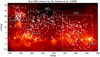 |
Fig. 1 Sco OB2 census by de Zeeuw et al. (1999) in Galactic coordinates. The white triangles mark the 521 identified HIPPARCOS members. The boundaries of the three subgroups are indicated by the dashed white lines: from left to right, Upper Sco (US), Upper Centaurus Lupus (UCL), and Lower Centaurus Crux (LCC) appear, respectively. The “new” subgroup Lower Sco is indicated by a dashed white circle; the position of the open cluster IC 2602 is displayed by a white diamond. The Ophiuchus star forming region is centered at the small white circle (l = 354°, b = 17°). The background image is taken from the Hα map of Finkbeiner (2003). |
2 Data processing
2.1 Data source
We obtained data from the Gaia Archive3 (see the ADQL code in Appendix A) and reduced the size of the data by cutting off as many field stars as possible in proper motion, position, and parallax space based on the prior knowledge we have on Sco OB2 (de Zeeuw et al. 1999; Rizzuto et al. 2011); see Section 2.4 for more details.
2.2 Astrometry data quality filters
The Gaia DR2 catalog (Gaia Collaboration 2018) provides a goodness-of-fit indicator goodness_of_fit_al for the exclusion of low-quality astrometric measurements. However, this parameter is found to be inadequate for our purposes (Lindegren et al. 2018). We follow the recipe provided in the technical note of Lindegren et al. (2018) as described in the following paragraphs.
Instead of using the goodness-of-fit indicator, we built our filter from the “Unit Weight Error” (UWE), which is not provided in the catalog of Gaia DR2,
![Mathematical equation: $\[\mathrm{UWE}=\sqrt{\frac{\chi^2}{N-5}}\]$](/articles/aa/full_html/2025/04/aa44011-22/aa44011-22-eq1.png) (1)
(1)
where χ2 is the astrometric chi-square value (column name astrometric_chi2_al in the catalog), and N is the number of good observations (astrometric_n_good_obs_al). The UWE needs to be renormalized to the Re-normalized UWE (RUWE),
![Mathematical equation: $\[\text { RUWE }=\frac{\mathrm{UWE}}{u_0(G, C)},\]$](/articles/aa/full_html/2025/04/aa44011-22/aa44011-22-eq2.png) (2)
(2)
where G is the apparent magnitude (phot_g_mean_mag), C is the color (GBP − GRP) (bp_rp), and u0 is the re-normalization function using the extra data table provided on the Gaia website4. We use the recommended filter condition RUWE < 1.40 as our selection standard for good astrometric data in this work. In addition, we exclude the stars with poor parallax quality, that is, only include the candidates with (σϖ/ϖ) ≤ 0.2, preventing complications related to the distance estimates (Bailer-Jones 2015).
2.3 Correction on the standard errors
The astrometric standard errors in position, parallax and proper motion of Gaia DR2 are underestimated, resulting in an overestimation of the velocity dispersion; thus, we correct the standard errors of parallax and proper motion using the recipe provided by Lindegren’s slides5,
![Mathematical equation: $\[\sigma_{\mathrm{ext}}=\sqrt{k^2 \sigma_{\mathrm{int}}^2+\sigma_s^2},\]$](/articles/aa/full_html/2025/04/aa44011-22/aa44011-22-eq3.png) (3)
(3)
where σint is the “internal standard error” of an astrometric parameter (position, parallax, or proper motion) given as the standard error in the Gaia catalog, σs is the empirical systematic error for the parameter, and k is the factor to inflate the internal error. The inflated internal error and the systematic error combine to give the “external standard error”, σext, which is what we use in our membership analysis instead of the internal standard error provided in the catalog. The correction parameters k and σs vary with brightness (different for bright (G < 13 mag) and faint (G ≥ 13 mag) stars) as well as with the type of observable (in our case, ϖ, μα* and μδ). The k and σs values used in our correction are listed in Table 1, where the values are taken from the aforementioned slides of Lindegren, except for k = 1.743 from Brandt (2018).
2.4 Preliminary candidates
We reduced the number of candidates by cutting out stars that are unlikely to be members according to their coordinates (Table 2a), parallax (Table 2-a), and proper motion (Table 2b, c). The association forms a banana-shaped concentration in the tangential velocity space6 vα*-vδ, where vα*, vδ are the velocities converted from proper motion μα* and μδ in the direction of right ascension (α) and declination (δ), respectively (Fig. 2). The cut in astrometric space is made according to Table 2. Each row of the table is a record of boundaries of a particular region in space (l, b in degree and ϖ in mas) or tangential velocity (vα*, vδ, and ![Mathematical equation: $\[v_{\|}=\left(v_{\alpha *}^{2}+v_{\delta}^{2}\right)^{1 / 2}\]$](/articles/aa/full_html/2025/04/aa44011-22/aa44011-22-eq4.png) in km s−1). For example, the region s1 is defined as a region between 285° ≤ l ≤ 360°, −10° ≤ b ≤ 30°, and 5 ≤ ϖ ≤ 11 mas. The tangential velocity regions v1 and v2 are circles defined by a center (c(vα*), c(vδ)) and a radius rv in the tangential velocity space. The stars within the regions form subsets {si, vi} which are combined by a series of Boolean operations. The operator symbols are represented as s1 ∪ s2 for union between s1 and s2, s1 ∩ s2 for intersection between s1 and s2, and
in km s−1). For example, the region s1 is defined as a region between 285° ≤ l ≤ 360°, −10° ≤ b ≤ 30°, and 5 ≤ ϖ ≤ 11 mas. The tangential velocity regions v1 and v2 are circles defined by a center (c(vα*), c(vδ)) and a radius rv in the tangential velocity space. The stars within the regions form subsets {si, vi} which are combined by a series of Boolean operations. The operator symbols are represented as s1 ∪ s2 for union between s1 and s2, s1 ∩ s2 for intersection between s1 and s2, and ![Mathematical equation: $\[\bar{s}\]$](/articles/aa/full_html/2025/04/aa44011-22/aa44011-22-eq5.png) for the complementary of set s. The set of preselected candidates is thus
for the complementary of set s. The set of preselected candidates is thus ![Mathematical equation: $\[\left(s_{1} \cup s_{2}\right) \cap\left(\overline{s_{3} \cup s_{4} \cup s_{5}}\right) \cap\left(v_{1} \cap v_{4} \cap v_{5} \cap\left(\overline{v_{2} \cup v_{3}}\right)\right)\]$](/articles/aa/full_html/2025/04/aa44011-22/aa44011-22-eq6.png) .
.
Fig. 2 demonstrates the different filters and cuts applied to preselect the data. The velocity cut regions are specifically designed to exclude the majority of field stars while to retain as many potential members as possible. IC 2602 is also included in the preselection, as its tangential velocity appears at the end of the Sco OB2 velocity stream (Fig. 2, last row, right panel, the small concentration at the top is IC 2602).
2.5 Preselection results from Gaia EDR3
We are aware that Gaia (Early) Data Release 3 (Gaia EDR3 Gaia Collaboration 2021 and Gaia DR3: Gaia Collaboration 2021) offers higher quality astrometry than Gaia DR2. A quick check (see details in the next paragraph) shows that the same preselection criteria applied to the EDR3 sample result in a smaller sample size (from 29908 in DR2 to 23743 in EDR3). This difference will not affect our main results as the missing stars are mainly the field stars in the Galactic disk. In fact, the increased accuracy in proper motion and parallax in EDR3 helps to concentrate the field stars in the transverse velocity space, making our preselection criteria more effective at removing the field stars from the sample.
We have produced the preselection sample with Gaia EDR3 using the same selection criteria as in Section 2, that is, RUWE <1.4, ϖ/σϖ ≥ 5, and the spatial and transverse velocity cuts. Fig. C.1 shows the results that can be compared with Fig. 2. A notable difference is that the preselection sample of EDR3 contains ~6000 sources fewer than that of DR2. Comparing the panels in the transverse velocity space in the two figures, one can notice that the large concentration of velocities by the field stars is more concentrated in EDR3 than in DR2, making the Sco OB2 structures more prominent in this space. Thus our cut in velocity space becomes more effective in removing the field stars, resulting in the smaller number of preselected candidates. This can be confirmed by comparing the bottom panels in l − b space; in the DR2 sample the horizontal parallel structure formed by the field stars above and below the Galactic plane is still visible, whereas in the EDR3 sample, this structure disappears, and the Sco OB2 substructures are more prominent. In conclusion, using Gaia EDR3 for this work would help to reduce the field stars more effectively prior to the membership selection thanks to the higher accuracy in parallax and proper motion; however, this is not expected to lead to a significant change in our membership selection7.
Boundary conditions of the preliminary candidate selection.
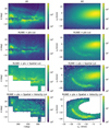 |
Fig. 2 Different stages applied to preselect the data. Left column: stellar density maps in the l-b plane; Right column: stellar density maps in the transverse velocity plane. The color bars show the color coding of point-source density in log-scale. Row 1: all the candidates downloaded from the Gaia Archive. Row 2: after applying the filter of RUWE < 1.4 and (σϖ/ϖ) < 0.2. Row 3: in addition to the previous filters, apply all the conditions in the first table of Table 2. Row 4: in addition to the previous cuts, apply all the conditions in the second and third table in Table 2. This set contains the preselected candidates. |
3 Membership analysis
We employed a modified kinematic modeling method following Lindegren et al. (2000). The method compares a group-model-predicted proper motion with the observed proper motion and estimates the membership probability of a candidate star based on the difference between the two. The mathematical details are worked out in the remainder of this section.
3.1 The velocity model of the co-moving group
Previous studies of Sco OB2, such as presented by Blaauw (1964b) and de Zeeuw et al. (1999), treated the subgroups as separate entities, while Rizzuto et al. (2011) attempted to identify the association as a continuous stream. As shown in Fig. 2, the potential members of Sco OB2 are continuously distributed in tangential velocity space as well as in real space. Thus, it is not physically appropriate to split the moving group into subgroups by group velocity, which depends on the selection of subgroup boundaries in velocity space.
Unlike Rizzuto et al. (2011) who built the velocity model as a function of Galactic longitude l, we construct our model velocity vg = (vx,g, vy,g, vz,g)⊤ as a function of spatial coordinate x = (x, y, z)⊤8 in the International Celestial Reference System (ICRS). Because the variation of velocity with respect to the space coordinates in the region is small (<10 km s−1 per 100 pc in each velocity component in each spatial direction), we choose the three components vx,g, vy,g, vz,g as linear functions of the space coordinates:
![Mathematical equation: $\[\left[\begin{array}{l}v_{x, g} \\v_{y, g} \\v_{z, g}\end{array}\right]=\left[\begin{array}{llll}u_{x x} & u_{x y} & u_{x z} & u_{0 x} \\u_{y x} & u_{y y} & u_{y z} & u_{0 y} \\u_{z x} & u_{z y} & u_{z z} & u_{0 z}\end{array}\right]\left[\begin{array}{l}x \\y \\z \\1\end{array}\right],\]$](/articles/aa/full_html/2025/04/aa44011-22/aa44011-22-eq9.png) (4)
(4)
where uξη (ξ, η ∈ {x, y, z}) is the partial derivative of velocity component vξ with respect to coordinate η, and u0ξ is the velocity component vξ at x = (0, 0, 0)⊤. For simplicity in notation, we rewrite Eq. (4) as
![Mathematical equation: $\[\boldsymbol{v}_g=F \cdot \boldsymbol{x}_4,\]$](/articles/aa/full_html/2025/04/aa44011-22/aa44011-22-eq10.png) (5)
(5)
where x4 = (x, y, z, 1)⊤ and F is the matrix transforming x4 into vg.
In order to project the predicted velocity vg with a given sky coordinate (α, δ) and parallax ϖ to proper motion and radial velocity, the normal triad is needed. They are normalized vectors as a function of spherical coordinate (α, δ), pointing to the corresponding tangential and radial directions. The components ![Mathematical equation: $\[\hat{p}, \hat{q}, \hat{r}\]$](/articles/aa/full_html/2025/04/aa44011-22/aa44011-22-eq11.png) are defined as
are defined as
![Mathematical equation: $\[\hat{p}=\left[\begin{array}{c}-\sin \alpha \\\cos \alpha \\0\end{array}\right], \hat{q}=\left[\begin{array}{c}-\sin \delta \cos \alpha \\-\sin \delta \sin \alpha \\\cos \delta\end{array}\right], \hat{r}=\left[\begin{array}{c}\cos \delta \cos \alpha \\\cos \delta \sin \alpha \\\sin \delta\end{array}\right],\]$](/articles/aa/full_html/2025/04/aa44011-22/aa44011-22-eq12.png) (6)
(6)
and the transformation from spherical coordinates (α, δ, ϖ) to Cartesian (x, y, z) can be expressed as
![Mathematical equation: $\[\left[\begin{array}{l}x \\y \\z\end{array}\right]=\frac{\mathrm{A}}{\varpi} \cdot\left[\begin{array}{c}\cos \delta \cos \alpha \\\cos \delta \sin \alpha \\\sin \delta\end{array}\right],\]$](/articles/aa/full_html/2025/04/aa44011-22/aa44011-22-eq13.png) (7)
(7)
where A = 4.74047 yr km s−1 is the astronomical unit converted into a unit for easier calculation. Using Eqs. (6) and (7) on Eq. (5), we obtain the predicted proper motion and radial velocity:
![Mathematical equation: $\[\left[\begin{array}{c}\mu_{\alpha *, g} \\\mu_{\delta, g} \\v_{r, g}\end{array}\right]=\left[\begin{array}{ccc}p_x \varpi / A & p_y \varpi / A & p_z \varpi / A \\q_x \varpi / A & q_y \varpi / A & q_z \varpi / A \\r_x & r_y & r_z\end{array}\right] \cdot F \cdot \frac{\mathrm{~A}}{\varpi} \cdot\left[\begin{array}{c}\cos \delta \cos \alpha \\\cos \delta \sin \alpha \\\sin \delta \\\varpi / A\end{array}\right].\]$](/articles/aa/full_html/2025/04/aa44011-22/aa44011-22-eq14.png) (8)
(8)
In addition, we assume that the velocity dispersion is the same across the whole group but anisotropic; thus the matrix of velocity dispersion S is defined as:
![Mathematical equation: $\[S_g=\left[\begin{array}{ccc}\sigma_{x, g}^2 & 0 & 0 \\0 & \sigma_{y, g}^2 & 0 \\0 & 0 & \sigma_{z, g}^2\end{array}\right],\]$](/articles/aa/full_html/2025/04/aa44011-22/aa44011-22-eq15.png) (9)
(9)
where σξ,g (ξ ∈ {x, y, z}) is the velocity dispersion in direction ξ and the subscript g stands for group. The off-diagonal terms are set to zero assuming that the dispersion components have no correlation with each other.
3.2 The velocity model of nonmembers
In order to effectively discard nonmembers, we also introduce a velocity model for the “field stars”, that is, the stars with motions not compatible with the moving group model. We assume that the nonmembers follow a random motion, and can be described as a co-moving group with a large velocity dispersion. Therefore the model is simply a single velocity vector
![Mathematical equation: $\[\boldsymbol{v}_f=\left(v_{x, f}, v_{y, f}, v_{z, f}\right)^{\top},\]$](/articles/aa/full_html/2025/04/aa44011-22/aa44011-22-eq16.png) (10)
(10)
and likewise one can transform the velocity to proper motion using the normal triad:
![Mathematical equation: $\[\boldsymbol{\mu}_f=\left(\mu_{\alpha *, f}, \mu_{\delta, f}\right)^{\top}=(\varpi / A)\left(\hat{p} \cdot \boldsymbol{v}_f, \hat{q} \cdot \boldsymbol{v}_f\right)^{\top}.\]$](/articles/aa/full_html/2025/04/aa44011-22/aa44011-22-eq17.png) (11)
(11)
We also assume an anisotropic velocity dispersion for the non-members:
![Mathematical equation: $\[S_f=\left[\begin{array}{ccc}\sigma_{x, f}^2 & 0 & 0 \\0 & \sigma_{y, f}^2 & 0 \\0 & 0 & \sigma_{z, f}^2\end{array}\right],\]$](/articles/aa/full_html/2025/04/aa44011-22/aa44011-22-eq18.png) (12)
(12)
where the subscript f stands for field.
3.3 Likelihood function of kinematic modeling
We apply the kinematic modeling method from Lindegren et al. (2000). For each star’s observed proper motion μi = (μα*,i, μδ,i)⊤ we compare it with both model predictions μg and μf; assuming that the difference Δμi,k = μi − μk, where k ∈ {g, f}, follows a Gaussian distribution, the likelihood function is thus defined as:
![Mathematical equation: $\[p_{i, k}\left(\boldsymbol{\mu}_k \mid \boldsymbol{\mu}_i\right)=\frac{1}{2 \pi\left|D_i\right|} \exp \left(-\Delta \boldsymbol{\mu}_{i, k}^{\top} D_i^{-1} \Delta \boldsymbol{\mu}_{i, k} / 2\right),\]$](/articles/aa/full_html/2025/04/aa44011-22/aa44011-22-eq19.png) (13)
(13)
where the variance matrix Di
![Mathematical equation: $\[\begin{aligned}D_i=C_i & +\left[\begin{array}{ll}\hat{p}_i^{\top} S \hat{p}_i & \hat{p}_i^{\top} S \hat{q}_i \\\hat{q}_i^{\top} S \hat{p}_i & \hat{q}_i^{\top} S \hat{q}_i\end{array}\right]\left(\frac{\varpi_i}{\mathrm{~A}}\right)^2 \\& +\left[\begin{array}{cc}\left(\hat{p}_i \cdot \boldsymbol{v}_{\boldsymbol{k}}\right)^2 & \left(\hat{p}_i \cdot \boldsymbol{v}_{\boldsymbol{k}}\right)\left(\hat{q}_i \cdot \boldsymbol{v}_{\boldsymbol{k}}\right) \\\left(\hat{p}_i \cdot \boldsymbol{v}_{\boldsymbol{k}}\right)\left(\hat{q}_i \cdot \boldsymbol{v}_{\boldsymbol{k}}\right) & \left(\hat{q}_i \cdot \boldsymbol{v}_{\boldsymbol{k}}\right)^2\end{array}\right]\left(\frac{\sigma_{\varpi, i}}{\mathrm{~A}}\right)^2\end{aligned}\]$](/articles/aa/full_html/2025/04/aa44011-22/aa44011-22-eq20.png) (14)
(14)
contains three terms. The first term Ci is the covariance matrix of the observed proper motion, the second term represents the variance of the proper motion due to the intrinsic velocity dispersion, and the last term is the variance caused by the uncertainty in parallax.
The total likelihood of both the group (where k = g) and the field (where k = f) models being consistent with the observation of star i is
![Mathematical equation: $\[\Phi_i=\lambda_g \cdot p_{i, g}\left(\boldsymbol{\mu}_g \mid \boldsymbol{\mu}_i\right)+\left(1-\lambda_g\right) \cdot p_{i, f}\left(\boldsymbol{\mu}_f \mid \boldsymbol{\mu}_i\right),\]$](/articles/aa/full_html/2025/04/aa44011-22/aa44011-22-eq21.png) (15)
(15)
where λg is the combination factor. With N candidates containing a group of co-moving stars and field stars of random motion, the set of optimized model parameters (F, Sg, vf, Sf, λg) should maximize the product ![Mathematical equation: $\[{\prod}_{i=1}^{N} \Phi_{i}\]$](/articles/aa/full_html/2025/04/aa44011-22/aa44011-22-eq22.png) .
.
Using the total likelihood Φi as a normalization factor, we can define the probability function of the i-th star being in the group
![Mathematical equation: $\[p_i(\text { in group })=\frac{\lambda_g \cdot p_{i, g}\left(\boldsymbol{\mu}_g \mid \boldsymbol{\mu}_i\right)}{\Phi_i}.\]$](/articles/aa/full_html/2025/04/aa44011-22/aa44011-22-eq23.png) (16)
(16)
The probability of the star belongs to the field is thus
![Mathematical equation: $\[p_i(\text { in field })=\frac{\left(1-\lambda_g\right) \cdot p_{i, f}\left(\boldsymbol{\mu}_f \mid \boldsymbol{\mu}_i\right)}{\Phi_i}=1-p_i(\text { in group }).\]$](/articles/aa/full_html/2025/04/aa44011-22/aa44011-22-eq24.png) (17)
(17)
The probability threshold on pi (in group) to classify a star as a member of Sco OB2 should be at least 0.5 by definition; above the lower bound, it can be set according to the need of the analysis. On the one hand, a high probability threshold selects only the “purest” members that are the best fit to the group’s kinematic model; this is a useful approach when determining astrophysical properties, such as stellar age. On the other hand, a low probability threshold keeps more candidates in the pool, enabling a larger sample size and making a sample closer to completeness. In this work, we use pi (in group) ≥ 0.95 as the condition for a star to be a member.
List of optimized parameters from the velocity model.
3.4 Results
We identified 5106 stars out of 26017 candidates as members of Sco OB2. The numerically optimized parameters of our velocity model in Eqs. (4), (9), (10), and (12) are listed in Table 3. The combination factor λg in Eq. (15) is 0.44. The uncertainty of the optimization results for the matrix elements in Eq. (4) has an order of magnitude 10−8 for uij and 10−6 for ui0; the uncertainty for the rest of the parameters ranges from ~10−7 to 10−5.
In Fig. 3, the selected members are shown in proper motion – parallax space. The left panel shows the stars in proper motion space: right ascension (horizontal axis) and declination (vertical axis). The objects with a membership probability ≥0.95 are colored from black to orange, the brighter the color, the higher the probability; the remaining objects are colored gray. The inset in the middle panel incorporates the color scale representing membership probability. The main plot of the middle panel shows the relation between the parallax and the total proper motion. It should be a linear relation given a nearly constant tangential velocity. The right panel of Fig. 3 displays the smoothed parallax number density distribution of the members:
![Mathematical equation: $\[n(\varpi)=\sum_{i=1}^{N_{\mathrm{Star}}} g\left(\varpi_i, \sigma_{\varpi, i}\right),\]$](/articles/aa/full_html/2025/04/aa44011-22/aa44011-22-eq25.png) (18)
(18)
where g(ϖi, σϖ,i) for star i is a Gaussian distribution function using the parallax central value ϖi as mean, and the standard deviation σϖ,i as the scale factor:
![Mathematical equation: $\[g\left(\varpi_i, \sigma_{\varpi, i}\right)=\frac{1}{\sqrt{2 \pi} \sigma_{\varpi, i}} \exp \left[-\frac{1}{2}\left(\frac{\varpi-\varpi_i}{\sigma_{\varpi, i}}\right)^2\right].\]$](/articles/aa/full_html/2025/04/aa44011-22/aa44011-22-eq26.png) (19)
(19)
The parallax distribution peaks at ~7 mas (≈140 pc), with a secondary peak at ~5.5 mas (≈180 pc), providing a glimpse of the substructure of Sco OB2 in the radial direction. Being less than 200 pc away and with σϖ/ϖ ≤ 0.2, the bias in distance introduced by inverting the parallax and truncating the sample, is minimal (Bailer-Jones 2015; Luri et al. 2018).
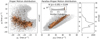 |
Fig. 3 Result of membership selection. The members are represented by the points color coded according to membership probability from 0.95 to ~0.98 (black to orange). The brighter the color, the higher the probability. The nonmembers are colored gray. Left panel: members and nonmembers plotted in proper motion space (equatorial coordinates). Middle panel: members and nonmembers plotted in parallax – total proper motion space. The inset shows a histogram of membership probability. Right panel: smoothed parallax distribution of the members. The horizontal axis shows the number density, while the vertical axis displays the parallax. |
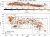 |
Fig. 4 Sky map presenting the members of Sco OB2 based on our analysis. Upper panel: the distance (1000/ϖ) of the members against Galactic longitude l. Lower panel: members shown in the Galactic coordinate plane. The subgroup boundaries in de Zeeuw et al. (1999) are marked by the black dashed lines. In both panels, the membership probability is color coded as represented by the color bar. The open cluster IC 2602 is shown as a black diamond; according to our analysis, it is not part of Sco OB2. |
4 Subgroup structure in Sco OB2
4.1 The sky map of Sco OB2
Fig. 4 shows the outcome of the membership analysis of Sco OB2. The color code indicates the membership probability with 95% as the lowest value, and the brighter the color, the higher the probability. At first sight, there are two major concentrations in the field of view, roughly centered at (l, b, d) = (350°, 20°, 150 pc) and (345°, 5°, 175 pc), where d = 1000/ϖ (pc). In terms of the subgroup structure of de Zeeuw et al. (1999), the first concentration corresponds to Upper Scorpius (US). The Upper Centaurus Lupus (UCL) subgroup includes the second major concentration that has been noticed earlier by de Bruijne (1999), Mamajek et al. (2013), Nguyen et al. (2013), Pecaut & Mamajek (2016), Röser et al. (2018) (as “V1062 Sco”) and by Damiani et al. (2019) (as “UCL-1”), respectively. In Gaia DR2 the over density is much more prominent than in the HIPPARCOS data. We confirm that this second major concentration is the same object as referred to in the mentioned works. We adopt the name “Lower Scorpius” (LS) for this concentration, as in Mamajek et al. (2013); Nguyen et al. (2013); Pecaut & Mamajek (2016).
The other subgroups are not as well defined as US and LS. By eye we can observe smaller overdensities across the Sco Cen region. Thus we need the help of a computer algorithm to define these overdensities in a reproducible manner.
4.2 Define spatial subgroups with DBSCAN
As the overdensities in Fig. 4 are irregularly shaped in three-dimensional space, simple geometrical boundaries are not sufficient to properly define the subgroup structure. We apply the Density-Based Spatial Clustering of Applications with Noise (DBSCAN) algorithm in scikitlearn9 to the 3D positions of the members to quantify the clustering.
The DBSCAN algorithm looks for clustering of points, given a maximum distance ϵ between neighbors, and a minimum number of points Nmin required to define a cluster. In this work, we move the 3D positions (Cartesian coordinates (x, y, z) in pc) of the members of Sco OB2 from Galactic cartesian coordinates to standardized coordinates (i.e., translate the coordinates so that the mean position sits on the origin). The standard coordinates Xs are calculated with the formula Xs = X − U, where X represents the input coordinates, U the mean of all X. We do not rescale the distances according to their dispersion in the three dimensions because Sco OB2 is a physically elongated structure; compression by rescaling would introduce unnaturally close distances between the stars. Thus the coordinates are simply shifted to center around the origin. Then we choose ϵ = 0.2 and Nmin = 20 for the algorithm to run on our sample. These parameters are selected such that we are able to recover the known major substructures (e.g., Upper Sco) as well as minor substructures in UCL. The limit Nmin = 20 is imposed so that the age determination process can have a reasonable sized sample to work on.
The algorithm identifies 8 subgroups; we label them from 1 to 8, as shown in Table 410. The members that do not belong to any of the clumps are labeled 0 (gray dots in Figs. 5 and 6). We assign the latter members to the “Sco OB2 Halo” population, or “Halo” in short. We note that that the Halo stars are still members of Sco OB2, they are just not meeting our criteria for the algorithm to be in one of the 8 subgroups. Since DBSCAN is a deterministic algorithm, the user can precisely reproduce the result using the table and code we provide in the Appendix. Figs. 5 and 6 show the subgroups in different colors in spherical and cartesian coordinates, respectively.
We can now name the newly defined subgroups according to conventions. Among the eight subgroups, it is easy to confirm that group 1 (blue) is LS and group 3 (green) is US. The two most prominent spatial concentrations are recovered by the algorithm; US gets 1137 members, the highest of all subgroups, and LS includes 487 members, making it the third most populated group. Group 6 (brown), the second subgroup in number, is contained by the LCC region; it hosts 1048 stars. Unlike the other subgroups, it has a prolonged shape. We name it LCC in this work to stay consistent with the historical convention. These three most populated subgroups form three anchor-points in space serving as the outline of the association. Group 4 (red), 5 (purple), and 7 (pink) consist of 157,202, and 39 stars, respectively, forming a string of small clumps in the Lupus region filling the space on the plane defined by US, LS and LCC (Fig. 7). Group 2 (orange) is located at about the same distance as LS (~175 pc), further than the other components of Sco OB2. It contains only 40 members, and is an outlier with respect to the plane formed by the major subgroups. As these four subgroups (groups 2, 4, 5, 7) are found in the traditional UCL region, we name them from west to east as UCL-1 (group 7), UCL-2 (group 5), UCL-3 (group 4), and UCL-4 (group 2). Lastly, group 8 (dark gray) hides under the curve of LCC with only 25 stars, the smallest of all subgroups. It may constitute a subbranch of LCC, so it is named LCC-1.
Subgroups defined by the DBSCAN algorithm.
5 Kinematic properties
In this section, we discuss the subgroup structures in proper motion and radial-velocity space.
5.1 Proper motion and tangential velocity
The vector point diagrams in Fig. 8 show the proper motion in both the Galactic and ICRS coordinate frames. On the one hand, the ICRS projection makes the points to fan-out into a banana-like shape where one can easily discern the various subgroups of the association; on the other hand, all the points are more concentrated into one direction in the Galactic frame. Fig. 9 shows the proper motion vectors plot in the Galactic coordinate sky map, in which the arrows are indeed pointing to roughly the same direction. This is for a large part due to the reflected solar motion.
Fig. 10 compares our velocity model to the observed tangential velocities. The modeled tangential velocity vectors (blue points in panel c) for all candidates are obtained by projecting the model space velocity onto the position of all the candidate stars, as shown in Eq. (8) but without the term (A/ϖ). Sco OB2 forms a continuous region in tangential velocity space vα*-vδ (Fig. 10b), and the region can be represented by our linear velocity field model (Fig. 10c). This supports our strategy that the Sco OB2 region can be described with a continuous velocity model rather than with individual models of subgroups. The small over-densities within the high density area (revealed by the contours) correspond well with the spatial concentrations of US, LS, UCL-3, and LCC. However, this correspondence can be explained by a projection effect: these subgroups are well-separated in space. Thus, the coordinate transformation ends up with separating the subgroups into over-densities in the tangential velocity space as well. At the top of the diagrams, around (vα*, vδ) = (−12.5, 7.5) km s−1, IC 2602 forms a notable over-density separated from Sco OB2. It is not covered by the extent of the group model, but partially overlaps with the field model; therefore this cluster did not make it into the final list of our census.
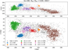 |
Fig. 5 Subgroups identified by DBSCAN in Galactic coordinates. The upper panel shows distance against Galactic longitude, the lower panel displays the Galactic latitude against longitude. The members of the subgroups are plotted in various colors (see in-set legend), and the members that do not belong to any subgroup (Halo stars) are colored gray. |
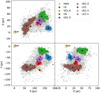 |
Fig. 6 Subgroups identified by DBSCAN in cartesian coordinates. The subgroup color code is the same as in Fig. 5. The black dots mark the mean position of the subgroups. The Sun’s position, in this case also the origin, is indicated with the usual (orange) symbol ⊙. |
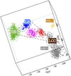 |
Fig. 7 Three dimensional view demonstrating the spatial structure formed by the subgroups. |
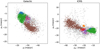 |
Fig. 8 Proper motion vector point diagrams in both Galactic (left panel) and ICRS coordinates (right panel). The subgroups are colored the same as Fig. 5. |
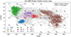 |
Fig. 9 Position and proper motion of the members in Galactic coordinates. The median proper motion across all members is ~30 mas yr−1, with a standard deviation of ~5.6 mas yr−1. The black arrows are the reflex of solar motion observed at parallax 7 mas on a grid of coordinate points. The solar velocity in the local standard of rest (U, V, W) = (9.6, 14.6, 9.3) km s−1 is taken from the local standard of rest in Reid et al. (2014). |
5.2 Radial velocity
Of the 5106 Sco OB2 members 616 (12%) have a measured radial velocity in Gaia DR2 (2871 of the 26017 preselected candidates). Gaia’s ability to obtain spectroscopic data from which the radial velocity can be determined, is limited to a certain magnitude range (Katz et al. 2018).
In Fig. 11, we plot the radial velocity as a function of Galactic longitude. We compare the radial-velocity component of our model to the observed radial velocity. In panel a, we plot the radial velocities against Galactic longitude for all 2871 preselected candidates (gray points). The contours indicate the density of the points within the area they enclose, the brighter the contour color, the higher the number density. The high density contours highlight a linear relation between radial velocity and Galactic longitude. Panel b shares the same dimensions and axes as panel a (so do panels c and d). In this panel we only plot the 616 members of Sco OB2 with error bars, using the same color coding for the subgroups as in Fig. 9, and, as a reference, the same contours for all the candidates as in panel a. The members overlap with the high density region (bright contours). There are a few members that fall outside the linear relation, which implies they may be interlopers. We discuss these stars in detail in the next subsection.
In Fig. 11c, we project the model velocity onto the radial direction taking the positions of the members, and plotted as colored points according to the subgroups as in panel b (regardless whether the radial velocity for that object is observed). The predicted radial velocities are contained in the high density region in panel a. Since our membership selection method does not use the observed radial velocity to correct the model for the moving group, the lack of this constraint is reflected by the slight shift of the model with respect to the data. But the overlap between the model and the observed radial velocity shows that the model is able to implicitly make use of the constraint from the projection effect of proper motion on a large area of the sky, which in principle can be used to infer a moving group’s radial velocity (Lindegren et al. 2000). Finally, in panel d, we project the nonmember model onto all the candidates to obtain the modeled radial velocity for the nonmembers, plotted as red points. The model points also form a linear relation between radial velocity and Galactic longitude, but systematically miss the high density region by ~5 km s−1.
In summary, the radial velocity of Sco OB2 forms a continuous linear trend with Galactic longitude. The kinematic model reproduces the radial velocity data.
Fig. 12 shows the deviation of the observed radial velocity from the prediction by the kinematic model. Panel a displays the radial velocity as a function of Galactic longitude as in Fig. 11. The Sco OB2 members are plotted as black points with error bars, the nonmembers as gray points, the group model as blue points, and the field model as red points. The vertical axis of the plot is limited to the range (−50, 50) km s−1 for clarity. Three members lie out of this range with vrad −65.2, 56.9, and 70.5 km s−1, respectively. The observed relation between the radial velocity and Galactic longitude is largely due to the projected peculiar motion of the Sun. In order to estimate the radial velocity dispersion, we subtract the predicted radial velocity from the observed radial velocity, and present the difference in histograms in Fig. 12c. The entire sample is displayed in black, with the subgroups in color. After the subtraction, the samples show a clear peak. The peak of the distribution is not centered at zero velocity, but systematically shifted toward the positive side. In order to quantify the shift, we smooth the radial-velocity-deviation distribution profile with the measurement errors, the same way as in formula (19) for the parallax, and plot the smoothed distributions in Fig. 12d. The peak of the curve for the total sample is located at 2.2 km s−1. Thus, the kinematic model underestimates the projected radial velocity by 2.2 km s−1 for the Sco OB2 region at large. This value varies slightly with subgroup. The measured radial velocity dispersion is 8.3 km s−1. We list these values in Table 5 for each subgroup.
Most of the subgroups have a radial-velocity dispersion between 1 and 5 km s−1, while US and the Halo population have a dispersion over 9 km s−1. The situation in the Halo is expected as it is a collection of Sco OB2 members with less concentration than the subgroups. However, it is clear that Upper Sco, one of the major, spatially concentrated subgroups, has a significantly larger radial-velocity dispersion than the other subgroups. We return to this observation in the Discussion.
5.3 Discrepancy between predicted and measured space velocity
With the six-dimensional astrometric data (position, parallax, proper motion, and radial velocity) we can reconstruct the observed space velocity of the members, although only 616 stars are available in our sample. As mentioned in the previous subsection, the difference between the observed and model radial velocity can lead to uncertainties in predicting the space velocity, with which nonmembers with matching proper motions but deviating radial velocities would be identified as members. We attempt to measure the vectorial difference between the model (vp) and observed (vobs) velocities using two quantities: the relative amplitude of the vector difference ΔV = |vobs − vp|/|vp|, and the cosine of the angular difference cos(vobs, vp) = (vobs · vp)/(|vobs| · |vp|). When the observed and predicted velocity vectors share direction but differ in amplitude, ΔV can capture the total vectorial deviation from the prediction regardless of similarity in direction, while cos(vobs, vp) mainly focuses on the difference in direction. Both quantities are plotted in the histograms of Fig. 13.
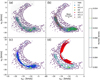 |
Fig. 10 Tangential velocity distribution of Sco OB2 in vα*-vδ space. All panels contain the same contours representing the number density of all candidates after preselection. Panel a: stellar density map of all candidates in the tangential velocity space. The darker the color, the higher the density. The high density area forms a curved shape. Panel b: plot of the members where all the subgroups are colored differently. The members overlap with the high density area. The subgroups together form a continuous distribution in the tangential velocity space, thus there is no incentive to separate Sco OB2 into subgroups based on transverse velocity distinctions. The mean error bar is indicated with a black cross. The size of the mean error is ~0.3 km s−1 for both dimensions. Panel c: plot of the group model velocities, well overlapping with the high density area. The model shows that the velocity of Sco OB2 can be described as one continuous velocity field instead of multiple subgroups with distinct velocities. Panel d: plot of the field model velocities. It does not directly cover the nonmembers in this diagram, but with the help of a very large velocity dispersion (~20–100 km s−1) it is adequate to represent the nonmembers. |
5.4 Estimating the number of interlopers
In the histogram of ΔV (Fig. 13, top panel) the majority of the values are below 0.5, and the main peak has a cut-off around 0.75 (vertical dashed line). There are 28 stars out of 616 with ΔV ≥ 0.75. The majority of the angular difference cos(vobs, vp) (Fig. 13, bottom panel) is above 0.8 (marked by the vertical dashed line). There are 25 stars out of 616 which have cos(vobs, vp) ≤ 0.8. The distributions of both quantities indicate that for most of the members good correspondence is obtained between model and observation. Combining the sets of members with either ΔV ≥ 0.75 or cos(vobs, vp) ≤ 0.8 results in 29 stars which have a large velocity discrepancy to our model. These are potential interlopers and thus nonmembers, 4.7% out of the sample of 616 stars. With this number we estimate a total of ~240 potential interlopers of the 5106 members.
Fig. 14 shows the 3D vector map of the radial velocity members of Sco OB2. The vector arrows are colored according to the subgroups as in Fig. 5, and the direction of motion of the entire sample is represented by a black arrow. We highlight the potential interlopers with red circles and arrows for ΔV ≥ 0.75, and orange diamonds for cos(vobs, vp) ≤ 0.8. Most of the potential interlopers pass both criteria, while four stars pass only the criterion ΔV ≥ 0.75. Further discussions of the interlopers in photometric space can be found in Sect. 7.3.
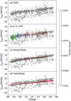 |
Fig. 11 Radial velocity vrad (km s−1) plotted as a function of Galactic longitude l (deg). The panels a, b, c, and d show the radial velocity of a subset of the stellar content as in Fig. 10, but in a different parameter space. The vertical axis of the plots is cropped down to (−50, 50) km s−1, while there are a few sources whose radial velocity can reach over 100 km s−1. Within our members, only one star in US exceeds this limit at ~70 km s−1. Panel a: plot of all preselected candidates with the contours showing the density. The brighter the color, the higher the density. The high density area follows a linear relation. Panel b: the radial velocity (with error bars) of the members. The subgroups are colored as in Fig. 5. The members overlap with the high density area except for a few outliers. All subgroups together form a continuous distribution, proving again that there is no incentive to separate Sco OB2 into subgroups based on a kinematical distinction. We note that most outliers are from the Halo population (gray points with error bars). Panel c: plot of the projected group model. The model points in this space are colored the same as their corresponding subgroups. The model overlays the high density area, but has a slight shift in radial velocity relative to the observations. The shift reflects the fact that our model does not use radial velocity to constrain the optimization process. Panel d: plot of the field model (red points). It separates from the high density zone just enough to generate the group-field model contrast. |
5.5 Kinematic substructure revealed by relative proper motion
Wright & Mamajek (2018) revealed kinematic substructure with relative proper motion of Sco OB2 in Gaia DR1/TGAS. They derived the relative proper motion by subtracting the bulk motions of the subgroups US, UCL, and LCC from the observed proper motions separately. The authors pointed out that each subgroup includes kinematic substructure. In this work we use our continuous kinematic model as the bulk motion for the entire Sco OB2 association to subtract from the observed proper motions. As our modeled velocity is a function of position, there is no need to divide the members into subgroups.
The relative proper motion vector map is shown in Fig. 15. The median position of a subgroup is indicated by a labeled black circle. The direction of the vector is color-coded as in the color wheel in the bottom left. The median size of the relative proper motion vectors is 1.34 mas yr−1. To visualize the regional orientation preference of the vectors more clearly, we show a median angle map of the relative proper motion in Fig. 16. The color of each pixel shows the median angle of the relative proper motion within a 2.5-degree radius, and a minimum of 20 stars within a range is required to produce a pixel. The color-coding is the same as in Fig. 15.
The relative proper motion is not random within Sco OB2. The whole association can be split into two major trends: one pointing “upward” (shades of purple/red) including LS, UCL-1, UCL-2, and UCL-3, and one pointing “downward” (shades of green) including US, LCC, UCL-4, and LCC-1. In particular, the green groups correspond well with US and LCC, distinguishing themselves from the neighboring LS and the various UCL subgroups. LS shares the direction of motion with the older UCL subgroups rather than with the youngest subgroup US (see Section 6 for age determination). The kinematic substructure within LCC is also revealed, which progresses from north to south, as was mentioned in the kinematic subgroup analysis by Goldman et al. (2018). Wright & Mamajek (2018) showed a similar distinction between the classical subgroups of US, UCL, and LCC in relative proper motions, except that US and LCC were shown to move in different directions compared to this work. The difference in the direction of relative motion can be the result of the difference in choosing the bulk motions between the two works: this work applies the linear velocity field as the bulk motion of Sco OB2, while Wright & Mamajek (2018) used bulk motions of individual subgroups.
In summary, the subtraction of the bulk motion predicted by the kinematical model reveals distinct dynamical substructures within a seemingly kinematically continuous association. The classical three-subgroup distinction US, UCL, and LCC by de Zeeuw et al. (1999) did reveal the kinematic substructure on a large scale. However, the actual kinematic boundaries are much more complex than the three proposed rectangular borders.
Radial velocity dispersion per subgroup.
6 Age estimation
The Sco OB2 association is not coeval. It consists of stars of different age (e.g., Preibisch & Zinnecker 2007; Pecaut & Mamajek 2016. In this section we first discuss the quality of the photometric data and how we control it, and then fit isochrones from the PAdova and TRieste Stellar Evolution Code (PARSEC) (Bressan et al. 2012; Chen et al. 2014, 2015; Tang et al. 2014; Marigo et al. 2017; Pastorelli et al. 2019) to the members. The isochrone fitting method adopted from Jørgensen & Lindegren (2005) is applied to estimate the age as well as the extinction of the subgroups. Additionally, we experiment with the technique from Pecaut & Mamajek (2016) using empirical isochrones to map the relative age of the region. One of the advantages of the empirical isochrones is that they are independent of stellar evolutionary models such as PARSEC.
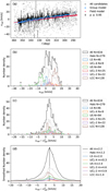 |
Fig. 12 The radial-velocity dispersion per subgroup in Sco OB2. Panel a: radial velocity vrad (km s−1) plotted as a function of Galactic longitude l (deg). All the candidates with a radial velocity measurement are colored gray; all the members with black error bars. The projected group model is in blue, and the field model in red. The radial velocity range of the plots is limited to (−50, 50) km s−1, while a few candidates exceed this limit. Panel b: the histograms of observed radial velocity per subgroup. The radial velocity dispersion of Sco OB2 is inflated by the projection effect, where the majority of the radial velocities are distributed within range (−10, 20) km s−1. Panel c: radial-velocity dispersion per subgroup. The radial velocity predicted by the kinematic model has been subtracted from the measured velocity. Panel d: the radial-velocity dispersion per subgroup, smoothed with measurement errors. The peak position is marked by a vertical line, and the peak value is listed in the legend. |
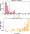 |
Fig. 13 Difference between the observed and model velocity vectors by the amplitude of vectorial difference (top panel) and angular difference (bottom panel). |
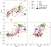 |
Fig. 14 Three dimensional vector field map, in Galactic cartesian coordinates, of the 616 members with a radial velocity in Gaia DR2. The members of the subgroups are colored (see inset). The black arrow shows the median motion of all members. The sources highlighted by red circles and arrows have ΔV ≥ 0.75 and orange diamonds have cos(vobs, vp) ≤ 0.8, and are potential interlopers. Most of them meet both conditions except four. |
6.1 The BP/RP color excess filter
We apply the BP/RP flux excess filter to exclude the sources with unreliable broadband magnitudes, in order to clean up the color-magnitude diagram (CMD). We did not apply this filter in the preselection process on the consideration that our method is solely based on astrometry, such that the results would not be directly affected by the quality of the photometry. In this section we follow the instructions of Evans et al. (2018) Section 8 to build the filter for Sco OB2.
Because the Gaia broad-band filters BP and RP slightly overlap, and together cover about the same wavelength range as the G band, the total flux of these two bands is expected to just exceed the flux of the G band. However, this excess can be inflated by various issues: for instance, the flux contamination in high density areas such as the center of a star cluster, where the light from surrounding sources can be mistakenly interpreted as the light of the target source. Thus we can compare the sum of the BP and RP flux with the G-band flux to verify the quality of the broad-band magnitudes of a given source. The flux excess factor C = (IBP + IRP)/IG (Evans et al. 2018), where IBP, IRP, and IG are the respective flux of the pass band, is listed in the Gaia Archive as phot_bp_rp_excess_factor. This factor is colordependent as shown in the left panel of Fig. 17. One can run a minimized χ2 fit on the relation with a quadratic function in the form of C = a + b (GBP − GRP)2 (black curve); the majority of the good-quality sources would be below the curve,
![Mathematical equation: $\[C<a+b(B P-R P)^2,\]$](/articles/aa/full_html/2025/04/aa44011-22/aa44011-22-eq28.png) (20)
(20)
where a and b are determined according to the specific sample. In our case, a = 1.22 and b = 0.04 are obtained by a χ-squared fit on the sample of all Sco OB2 members, different from the global fit in Evans et al. (2018). As a result, the filter excludes a few stars that are outside of the main-sequence, and 4652 stars remain after filtering (Fig. 17).
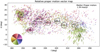 |
Fig. 15 Relative proper motion vectors in Sco OB2. The vectors are obtained by subtracting the predicted proper motion of the continuous velocity model from the observed proper motion. The direction of motion of the vector is color-coded as shown in the color wheel. Zero degrees is defined as pointing to the left of the plot, as the x-axis is flipped, and 90 degree pointing to the positive end of the y-axis. The median location of the subgroups is marked by a black circle with the subgroup name. |
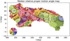 |
Fig. 16 Median angle map based on Fig. 15. Each pixel is color-coded by the median angle of the vectors within 2.5 degrees. A minimum of 20 stars is required to produce a colored pixel. The color code of the angle is the same as in Fig. 15. |
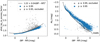 |
Fig. 17 BP/RP excess filter applied to the members. Left panel: the C−(GBP − GRP) relation. The majority of stars in Sco OB2 are below the fitted curve, thus the filter C < 1.22 + 0.04(GBP − GRP)2 selects the stars with good color quality, painted in blue. The stars excluded by the filter are colored in gray. Right panel: the color-magnitude diagram after filtering. The stars that passed the filter are plotted in blue, those excluded in gray. The black dashed line indicates the zero age main sequence (ZAMS) from the PARSEC model. |
6.2 Extinction
Sco OB2 is reported to have low to moderate interstellar extinction with generally AV < 1.5 mag (e.g., Pecaut & Mamajek 2016; Vos et al. 2011; de Geus 1992) assuming RV = 3.1. For a fraction of the sources in Gaia DR2 the extinction AG is inferred from its own broad-band photometry (Andrae et al. 2018). However, the extinction values (AG) are not meant to be applied directly onto individual stars, but only statistically as a group correction, assuming that the extinction of the group follows a Gaussian distribution (see Appendix E in Andrae et al. 2018). Besides, the estimate is biased against pre-main-sequence stars, such that these stars would be assigned a higher reddening value. Fig. 18 shows the sources in Sco OB2 with AG available in Gaia DR2 as a function of color (GBP − GRP) (top panel) and in a histogram (bottom panel), with the stars of (GBP − GRP < 1) colored blue, approximating the upper main-sequence population. The AG−(GB − GRP) relation shows a bi-modal behavior, where two clearly separated branches are present. In the histogram of AG, the distribution is even tri-modal (black histogram). This demonstrates that we are unable to apply the instruction of Andrae et al. (2018) to correct extinction for Sco OB2 based on these data. Therefore we estimate both the extinction and the age at the same time using isochrone fitting in this paper.
6.3 Isochrone model
We use multiple sets of the PARSEC isochrones11 (version 1.2 S Bressan et al. 2012; Chen et al. 2014, 2015; Tang et al. 2014; Marigo et al. 2017; Pastorelli et al. 2019). Each set of the isochrones incorporates an extinction value AV ranging from 0.0 to 1.1 mag with a step of 0.1 mag and an age ranging from 1 to 70 Myr with a step of 0.5 Myr. The choices for the other options on the web interface are listed in Table B.1. Since we cannot use the extinction AG from Gaia DR 2 for individual stars (Sect. 6.2), and the conversion from a known Aλ to AV is not trivial (Jordi et al. 2010), we treat the extinction as a free parameter when estimating the age. Based on our prior knowledge, the extinction to Sco OB2 is moderate, mostly with AV < 1.0 mag (Pecaut et al. 2012; Vos et al. 2011); therefore, the range of extinction covered by our isochrone grid should be sufficient.
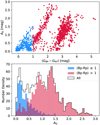 |
Fig. 18 Interstellar extinction as listed in Gaia DR2. Upper panel: bimodal distribution of the extinction in the sight lines toward Sco OB2 (AG versus (GBP − GRP)). The blue branch and red branch are produced by a cut at (GBP − GRP) = 1 mag. Lower panel: histogram of AG of the blue and red branch populations. |
6.4 Likelihood function of isochrone fitting
In this subsection, we discuss the isochrone fitting method. We adopt solar metallicity for the members, and make no prior assumption on the initial mass distribution. The star formation rate (SFR) is assumed to be flat. Thus, the prior probability functions in Jørgensen & Lindegren (2005) for metallicity, mass, and SFR are all constant.
In the color-magnitude parameter space, a 2-dimensional Gaussian function is defined for star i with observed color ci, magnitude mi, and corresponding formal standard errors (σci, σmi):
![Mathematical equation: $\[g_i(c, m)=\frac{1}{2 \pi \sigma_{c_i} \sigma_{m_i}} \exp \left\{-\frac{1}{2}\left[\left(\frac{c-c_i}{\sigma_{c_i}}\right)^2+\left(\frac{m-m_i}{\sigma_{m_i}}\right)^2\right]\right\}.\]$](/articles/aa/full_html/2025/04/aa44011-22/aa44011-22-eq29.png) (21)
(21)
Each point (c, m) in the color-magnitude space can then obtain an evaluation gi(c, m) that expresses how probable the true color c and magnitude m of the star are. Furthermore, an isochrone of age a and extinction ϵ can be described as a curve in the parameter space Ia,ϵ(c, m), thus the isochrone can obtain an evaluation on a set of sample points on the curve
![Mathematical equation: $\[G_i(a, \epsilon)=\sum_j g_i\left(c_j, m_j\right),\]$](/articles/aa/full_html/2025/04/aa44011-22/aa44011-22-eq30.png) (22)
(22)
where j is the index of a sample point on the curve Ia,ϵ(c, m). The function Gi(a, ϵ) (G-function) can be seen as the age-extinction likelihood function for star i.
For a given stellar population, we assume that the members are coeval and have similar extinction. Thus, multiplying all the G-functions of all the members should yield the age-extinction likelihood distribution of the population
![Mathematical equation: $\[G(a, \epsilon)=\prod_i G_i(a, \epsilon).\]$](/articles/aa/full_html/2025/04/aa44011-22/aa44011-22-eq31.png) (23)
(23)
The maximum of the likelihood function (amax, ϵmax) corresponds to the best fit isochrone age and extinction for the stellar population.
6.5 Uncertainty estimation with bootstrap
The isochrone fitting method of Jørgensen & Lindegren (2005) does not provide a useful constraint on the uncertainty of the age determination. The multiplication of a large number of G functions in practice only returns a nonzero maximum, while all other points obtain a value many orders of magnitude below the maximum and are rendered as zero due to the machine precision limit. To overcome this we apply a bootstrap resampling process to estimate the uncertainty of the results by slightly varying the population. We randomly redraw 90% of the stars in each DBSCAN subgroup for 200 times and fit the isochrones to obtain 200 sets of age and extinction estimates. The 90% redrawing ratio is chosen not only to allow for sample variations in the resampling process, but is also based on the conservative assumption that 10% of the members might be nonmembers, about twice as the estimated rate of interlopers in Sect. 5.4. The mean and standard deviation of the results are adopted as the age and extinction, and their uncertainties. In case that the bootstrap uncertainty is smaller than the grid size of the isochrone, 0.5 Myr for age and 0.1 mag for AV, respectively, we use the grid size as the adopted uncertainty.
6.6 Results of isochrone fitting
The age and interstellar extinction of the DBSCAN subgroups has been determined by fitting isochrones to individual members in the color-magnitude space, and by combining the individual G-functions. US is the youngest subgroup of Sco OB2 with an age of 11.5 ± 0.9 Myr and extinction AV = 0.4 ± 0.1 mag. LS is the second youngest with 14.0 ± 1.0 Myr, and LCC is the oldest among the three major concentrations US, LS, and LCC, at 17.5 ± 0.5 Myr with an extinction of AV = 0.2 ± 0.1 mag. The remaining subgroups have an age around 17.5 Myr, including the Halo stars, with relatively low AV. The subgroup with the most uncertain age is UCL-3 at the center of the field of Sco OB2, despite having more stars than UCL-1, UCL-4, and LCC-1. The small concentration UCL-4 has the highest extinction AV = 0.4 mag (Table 6). Fig. 19 shows the age-extinction distribution in the bootstrap results. For each subgroup the best fitting isochrone is plotted in a color-magnitude diagram (CMD) in Fig. 20.
6.7 Spatial variation of age
Pecaut & Mamajek (2016) derived an empirical isochrone for the Sco OB2 association and used it to map the relative age distribution. We reproduce this relative age map using the same technique with color (GBP − GRP) and magnitude MG, but without an extinction correction for individual stars; we assume that the mild extinction in this region has no differential effect on the loci of the subgroups in the CMD. An empirical isochrone of Sco OB2 is constructed by building a running mean curve in G-(GBP − GRP) space (Fig. 21, black line). There are four white dwarfs that remain after the membership selection and application of the photometric filters. They are most likely interlopers as the first white dwarfs are formed only after ~50 Myr, more than twice the age of Sco OB2. Thus the white dwarfs are excluded in this process. For pre-main sequence stars, the ones offset above the empirical isochrone are brighter than the stars of the same color, thus considered to be younger (colored in shades of blue); the stars below the isochrone are fainter and considered to be older (colored in shades of red). The stars that are close to the mean are colored yellow, transitioning to light blue and light red on each direction. The quantitative offset is defined in units of the running standard deviation from the running mean. The relation between the offset and the relative age holds only for pre-main sequence and young main sequence stars; as older, massive main sequence stars (in this case (GBP − GRP) < 0 mag) begin to evolve to the red giant phase, the relation is inverted. In this work, the majority of Sco OB2 members have a color of (GBP − GRP) > 0 mag, except for a few just over this boundary, and we can assume that this relation holds globally for all the members, and the few possibly deviant stars would not impose a difference on the results.
The spatial age maps12 (Figs. 22 and 23) display the median offset values in age, from blue (relatively young) to yellow (medium) to red (old), all using the same color scale shown in Fig. 21. Each pixel represents the median offset of stars in its surrounding circle of a certain radius (4° in the l-b maps in Fig. 22, 10 pc in the Cartesian maps in Fig. 23).
In order to find out whether the derived age distribution depends on the color of the stars, we split the population into two groups. One group with mostly main sequence (MS, (GBP − GRP) < 1 mag) stars and the other with mostly pre-main sequence (PMS, (GBP − GRP) > 1 mag) stars. The map of PMS is nearly identical to the overall map, while the MS maps show differences not only in reduced surface area (because of the lower stellar density) but also a slightly different age trend. The PMS map shows the age gradients consistent with our estimated ages of the DBSCAN subgroups, where the middle groups (around UCL) form the oldest part. The MS age map, however, shows a trend reflecting the previously believed age sequence in Sco OB2, which starts from the oldest subgroup LCC and progresses through UCL to the youngest US and the ρ Oph cloud (Blaauw 1991). This can be explained by the fact that in the HIPPARCOS era (and before), the brighter O- and B-type stars dominated the observable population.
In the gap between the subgroups LS, UCL-1, and UCL-2, we observe a region of young/bright stars (a light blue region between the red and yellow patches, see Fig. 23, top row), that coincides with the Lupus clouds (Luhman & Esplin 2020). This relatively young region appears to be squeezed away to the far-end of Sco OB2, which lends support to the star formation scenario of Krause et al. (2018).
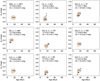 |
Fig. 19 Results of the bootstrap method to estimate the errors on age and extinction, per subgroup. Each circle centers on an age-extinction combination that occurs at least once in the 200 redrawn samples. The size of the circle is proportional to the number of occurrences. The biggest circle represents the most frequent age-extinction combination, and is marked with the highest occurrence number. The higher the number, the more yellow the circle. The inset lists the name of the subgroup, the number of stars, the median age and extinction, and the uncertainty. |
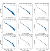 |
Fig. 20 Best fit isochrone per subgroup (black line) with the zero-age main sequence (ZAMS, dashed gray line) for reference. Only US and LS are significantly younger than the on average 17.5 Myr old population of Sco OB2. We note the in total four white dwarfs in the bottom left corner in the CMD of the Halo population and UCL-2; these are most likely interlopers. |
Results of the age and extinction estimate per subgroup.
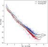 |
Fig. 21 Color-magnitude diagram showing the empirical isochrone produced by a running mean (black line), and offset isochrones defined in units of the running standard deviation (dashed line). The members brighter than the running mean (negative offset) are colored blue, the ones fainter (positive offset) colored red, and those close to the mean (near zero offset) colored yellow. |
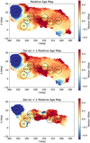 |
Fig. 22 Relative age map in Galactic coordinates. The color code corresponds to the median offset value within a 4° radius per pixel. The median position of the subgroup is indicated by a black circle labeled by name. The top panel is based on all members; the middle panel with only the members with (GBP − GRP) > 1 mag (mostly PMS stars); the lower panel with only the members with (GBP − GRP) < 1 mag (mostly MS stars). We find a strong correspondence with the result by Pecaut & Mamajek (2016). |
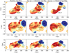 |
Fig. 23 Relative age map in cartesian coordinates. The color code corresponds to the median offset value within a 10 pc radius per pixel. The median position of the subgroup is indicated by a black circle labeled by name. The orange symbol ⊙ indicates the location of the Sun. The panels in the top, middle, and bottom rows show the views in X–Y, Y–Z, and X–Z space, respectively. The left diagrams are produced with all members; the middle ones with only the members with (GBP − GRP) > 1 mag (mostly PMS stars); and the right ones with only the members with (GBP − GRP) < 1 mag (mostly MS stars). |
7 Discussion
In this section, the Gaia DR2 census of Sco OB2 will be placed in context with earlier work and discussed in terms of star formation scenarios that have been proposed for this region in particular and the star forming regions near the Sun (within about 500 pc) in general.
7.1 Comparison of Gaia DR2 census to earlier work
The Gaia astrometric data excel in both quality and quantity compared to its predecessor, the HIPPARCOS catalogue (Perryman et al. 1997; van Leeuwen 2007). In the following we compare the Gaia DR2 census of Sco OB2 based on a kinematic modeling with earlier work.
We cross-matched the membership list of this work to that presented in three previous studies: de Zeeuw et al. (1999) (Z99), Rizzuto et al. (2011) (R11), and Damiani et al. (2019) (D19). Z99 and R11 are based on HipPARCOS, while D19 use Gaia DR2. In order to compare with Z99 and R11, we use the cross-match table provided by Marrese et al. (2018) to properly map the objects in HIPPARCOS to Gaia DR2 (see the ADQL code in Appendix A.4), with which we obtain the membership lists of Z99 and R11 with Gaia DR2 source identifiers. We identify the counterparts in Gaia DR2 for 515 out of 521 members in Z99, and 427 out of 436 members in R11.
Our preselected sample of 26 017 stars (no membership probability threshold applied) includes 366 and 321 members from Z99 and R11 (the “base subsets”), respectively. Thus about 30% of these two membership lists were rejected by our preselection procedure. When we cross-match the base subsets to our members with p ≥ 0.95, 157 stars are common with Z99, and 149 with R11, less than half of the corresponding original membership. As we decrease our membership probability threshold, the number of common stars increases for both censuses (see Table 7 column 2 and 3). The size of the common subsets does not seem big, but if we plot the assigned membership probability for both of the “base subsets” in histograms in Fig. 24, then we see that stars with p ≥ 0.95 in these subsets form a plurality, though not a majority.
In this work we choose p ≥ 0.95 to obtain a cleaner color-magnitude diagram for age determination. However, the stars with p ≥ 0.8 are good enough to be used as members in terms of consistent proper motions, if one needs a larger sample size with a larger deviation in proper motion. If we choose the threshold at 0.8, then, as shown in Fig. 24, the majority of both census are included as members.
Damiani et al. (2019) (D19) conducted a census of the Sco–Cen region by applying geometric boundaries in various parameter spaces, including proper motion, color and magnitude. D19 report a total of 14 437 stars in the association, including 350 stars in IC2602. Table B.2 shows the number of members from D19 recovered by this work at different thresholds of membership probability. Overall, 9957 stars (38%) of our 26 017 preselected sample appear in the list of D19. When we apply the membership probability threshold p ≥ 0.95, 4745 members are found in D19, which is 93% of the 5106 members in this work. Remarkably, only two stars of the overlapping population are marked as stars in IC2602 by D19. As we lower the membership threshold to 90%, the rate of overlap with D19 decreases to 88%. This trend continues down to 73% when the threshold is at 50%. The members of IC2602 start to appear in our membership list as well if we lower the membership probability threshold.
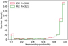 |
Fig. 24 Membership probability distribution of the members in Z99 (red) and R11 (green) in common with our preselected samples. The bin width in this plot is 0.05. |
Number of recovered members in Sco OB2 from various works.
7.2 The status of IC 2602
IC 2602 is an open cluster in the outskirts of subgroup LCC, and measured to have a similar proper motion to the members in Sco OB2. de Zeeuw et al. (1999) and Rizzuto et al. (2011) did not include it as a component of Sco OB2, while Bouy & Alves (2015) and Damiani et al. (2019) suggest that IC 2602 may be connected to the OB association. In our analysis we have included the region of IC 2602, but the membership criteria eventually rejected the open cluster as a part of the moving group. However, if we reduce the membership probability threshold from 95% to 90%, the open cluster appears in the candidate membership list. This explains why IC 2602 has been proposed as being part of Sco OB2, and that our strict kinematic membership threshold is capable of physically separating these two regions. Moreover, the age of the IC 2602 (~35 Myr, e.g., Bossini et al. 2019) is about twice that of LCC. Its proximity may have played a role in triggering the star formation process in Sco OB2. We further explore this hypothesis in Guo (2022).
7.3 Photometric properties of potential interlopers
In both Fig. 17 and the top left panel of Fig. 20, one can observe a trail of potentially main sequence stars below the pre-main sequence members of Sco OB2, in the range of (GBP − GRP) > 0.5 mag. Although they are identified as members based on our strict proper motion criteria, these stars are likely interlopers, as they appear older than the age of Sco OB2. In fact, the suspects of interloping stars due to deviating radial velocity in Sect. 5.2 are not randomly distributed in the color-magnitude diagram; they show a preference to occupy the main sequence rather than the pre-main sequence (red circles in Fig. 25). Due to the limited range of magnitude for the radial velocity members (orange points in Fig. 25) we are not able to show the tendency for (GBP − GRP) > 2 mag, however, one can speculate that the trend should continue if the same analysis can be done for the fainter members.
7.4 Expansion of the Sco OB2 association
Wright & Mamajek (2018) presented a kinematic study of the Sco OB2 region with the aim to test the hypothesis that OB associations are the expanded remnants of dense star clusters. They applied different methods on Gaia DR1/TGAS data, but did not find evidence for expansion of the subgroups. We have reconstructed the velocity field model by fitting it to our DR2 selected members. The model predicts a small divergence in velocity, ~0.03 km s−1, which is undetectable with the current data accuracy. Thus, we do not find evidence for or against spatial expansion of the moving group. The evaluation of the radialvelocity distribution of 616 members results in a typical velocity dispersion of a few km s−1, again showing no evidence for or against expansion of the subgroups.
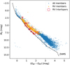 |
Fig. 25 Potential interlopers due to deviating radial velocity plotted in the color-magnitude diagram. The blue points show all the members of Sco OB2 that pass the BP/RP excess filter; the orange points are the members with radial velocity in Gaia DR2; the red circles mark the potential interlopers discussed in Sect. 5.2. For reference, the ZAMS model is included as a black dashed line. The data points are not corrected for extinction and reddening. |
7.5 Radial-velocity dispersion
In Sect. 5.2, we performed a consistency check on membership by analysing the radial-velocity measurements available for 616 members. The radial velocities show a clear trend with Galactic longitude, in line with membership of Sco OB2 and its motion with respect to the Sun. The radial-velocity dispersion per subgroup is a few km s−1, up to about 9 km s−1 for US.
However, the radial velocities of OB-type stars in Sco OB2 show a significantly larger spread, up to 40 km s−1 (Jilinski et al. 2006; Kharchenko et al. 2007). This discrepancy in radial-velocity dispersion is likely due to the high binary fraction (Kouwenhoven et al. 2007) and possibly pulsational (e.g., β Cephei-like) behavior of the OB-type members of Sco OB2.
7.6 The star formation history of Sco OB2
Since the first systematic studies of Sco OB2 it has been suggested that the star formation process in the Sco-Cen region is coordinated on a larger scale than the individual subgroups, and beyond, for example, on the scale of the Gould Belt. These regions are characterized by a relatively shallow age gradient over several hundreds of parsecs. The underlying physical explanation would be that star formation is triggered by external phenomena (such as the formation of stars in surrounding regions, the impact of the UV radiation fields of young massive stars and their powerful stellar winds, and supernovae) leading to triggered or sequential star formation (Blaauw 1964a; Preibisch & Mamajek 2008).
Recently, Krause et al. (2018) argued that the impact of star formation on a dense parental cloud results in superbubbles powered by massive stars that break out, surround and squash the denser parts of the gas sheet, and thus induce more star formation. They demonstrated that such a “surround and squash” scenario could well explain the observed spatial, kinematic, and age distribution of the stellar population of Sco OB2.
Kerr et al. (2021) applied the clustering algorithm DBSCAN to the young stellar population within a distance of 333 pc from the Sun using Gaia DR2, including Sco OB2. They find similar subgroup structure and corresponding ages as in this work, and identify a semicircular arc (the Libra-Centaurus arc) where the star formation process in Sco OB2 would have commenced. Furthermore, they find clear evidence for sequential star formation moving away from that arc.
Ratzenböck et al. (2023a) demonstrate that the star formation history of the Sco-Cen association is much more complicated than what one would expect in a sequential star formation scenario. They find evidence that most stars in this region formed about 15 Myr ago, while more recent star formation occurred in the Upper Sco area. They propose a feedback-driven star formation scenario alike the “Surround and Squash” scenario introduced by Krause et al. (2018), but then a more simple one: an octopus-like inside-out formation scenario.
8 Conclusions
In this work, we obtained a census of Sco OB2 in Gaia DR2 based on kinematic properties. Out of 26017 candidates 5106 are identified as members. The census recovers 157 members of de Zeeuw et al. (1999), 149 members of Rizzuto et al. (2011), and 4745 members of Damiani et al. (2019).
We investigated the substructure of Sco OB2 in three parameter spaces: spatial coordinates, proper motion-coordinates, and age-coordinates. A set of spatial subgroups is defined by using the DBSCAN algorithm, which recognizes the spatial subgroups in Sco OB2: Upper Scorpius (US), Lower Scorpius (LS), Lower Centaurus Crux (LCC), UCL-1 to 5, and LCC-1. They are named after the classical division names in this region from Blaauw (1964b) and de Zeeuw et al. (1999). We name the members that are not assigned a subgroup as the “Halo” group. We built the kinematic model for Sco OB2 as a linear velocity field, in which the space velocity of the group is not a constant but a function of spatial coordinates. We are able to use it to identify the membership of Sco OB2 without separating the association into arbitrary parts.
Kinematic substructures emerge when we subtract the observed proper motion of the members by the velocity model. The structure of the relative proper motion reveals patches of subgroups moving in different directions, and the boundaries of these subgroups appear to be similar to the spatial subgroup boundaries. We determined the age of the subgroups and found substructures in the relative age distribution. Both methods of age determination (PARSEC model isochrone fitting and empirical isochrone fitting) show that the oldest stars of Sco OB2 are found in the UCL region of the association; the youngest subgroup is US at 11.5±0.9 Myr, and the second youngest is LS at 14.0±1.0 Myr. The other subgroups all show a mean age of 17.5 Myr with various uncertainties. We are able to reproduce the age gradient given by Pecaut & Mamajek (2016). The age substructures resemble the major spatial subgroups in shape.
The substructure in the three aspects shows similarity with the star formation scenario proposed by Krause et al. (2018); in terms of the sequence of star forming events in Sco OB2, the stars in the UCL region was formed first, then came LCC, LS, and US into being. The triggering event of the first stars in UCL is yet unknown, while the proximity of IC 2602 appears to be a candidate to investigate. We address this issue in Guo (2022).
Data availability
We provide an electronic table containing all the candidate stars after the preselection and quality filtering, with Gaia DR2 designations and the probability values pi (in group), so that the reader can choose any probability threshold. Please contact This email address is being protected from spambots. You need JavaScript enabled to view it. for the data file.
Acknowledgements
This work is financially supported by NOVA. This work has made use of data from the European Space Agency (ESA) mission Gaia13, processed by the Gaia Data Processing and Analysis Consortium (DPAC)14. Funding for the DPAC has been provided by national institutions, in particular the institutions participating in the Gaia Multilateral Agreement. We thank Alex de Koter for carefully reading the manuscript and providing valuable feedback.
Appendix A Query code from the Gaia Archive
In this section we provide the ADQL code we use to obtain the data set from the Gaia Archive. Sco OB2 is a large region with millions of sources in the field. In order to avoid generating an overly large task for the Archive server and exceed the query time limit (2 hours for registered users), we separate the query into astrometry, photometry, and other cross-matching tasks to trim down the time taken by each task. The separate tables share the same sequence of entries but different columns; we recombine the files into one on our computer locally.
A.1 Astrometry
-- DR2 ScoCen_astrometry
SELECT designation,
ra, ra_error, dec, dec_error,
parallax, parallax_error,
pmra, pmra_error,
pmdec, pmdec_error,
ra_dec_corr,ra_parallax_corr,
ra_pmra_corr,ra_pmdec_corr,
dec_parallax_corr,dec_pmra_corr,
dec_pmdec_corr,parallax_pmra_corr,
parallax_pmdec_corr,pmra_pmdec_corr,
astrometric_primary_flag,
duplicated_source,
radial_velocity,radial_velocity_error,
l, b
FROM gaiadr2.gaia_source
WHERE (l>=285 AND l<=360
AND b>=-20 AND b<=30
AND parallax >= 4)
A.2 Photometry
-- DR2 ScoCen_photometry
SELECT designation, source_id,
phot_g_mean_flux,phot_g_mean_flux_error,
phot_g_mean_mag,
phot_bp_mean_flux,phot_bp_mean_flux_error,
phot_bp_mean_mag,
phot_rp_mean_flux,phot_rp_mean_flux_error,
phot_rp_mean_mag,
phot_bp_rp_excess_factor,bp_rp,bp_g,g_rp,
phot_variable_flag,
l,b,
teff_val,
teff_percentile_lower,teff_percentile_upper,
a_g_val,
a_g_percentile_lower,a_g_percentile_upper,
e_bp_min_rp_val,
e_bp_min_rp_percentile_lower,
e_bp_min_rp_percentile_upper,
radius_val,radius_percentile_lower,
radius_percentile_upper,
lum_val,
lum_percentile_lower,lum_percentile_upper
FROM gaiadr2.gaia_source
WHERE (l>=285 AND l<=360
AND b>=-20 AND b<=30
AND parallax >= 4)
A.3 Flags
This table is there to provide extra information on the entries of this work.
-- DR2 ScoCen_flags
SELECT gaia.designation,
gaia.priam_flags, gaia.flame_flags,
gaia.phot_variable_flag,
gaia.duplicated_source,
gaia.astrometric_gof_al,
gaia.astrometric_chi2_al,
gaia.astrometric_primary_flag,
gaia.astrometric_excess_noise,
gaia.astrometric_excess_noise_sig
FROM gaiadr2.gaia_source AS gaia
WHERE (l>=285 AND l<=360
AND b>=-20 AND b<=30
AND parallax >= 4)
A.4 HIPPARCOS NEW REDUCTION in Gaia DR2
The cross-match from the HIPPARCOS catalog to Gaia DR2 makes use of the corrected cross-matching table of Marrese et al. (2018). The table is uploaded to the archive as a user table by the author and named as user_dguo.hip2gdr2crossmatch in the code. The reader needs to adjust this part to their own use case.
-- Make the original hipparcos catalog list
-- crossmatched with gaia data
SELECT
gaia.designation, gaia.source_id, hip2.hip,
gaia.phot_g_mean_mag, gaia.phot_g_mean_flux,
gaia.phot_g_mean_flux_error,
gaia.phot_bp_rp_excess_factor,
gaia.phot_bp_mean_mag, gaia.phot_bp_mean_flux,
gaia.phot_bp_mean_flux_error,
gaia.phot_rp_mean_mag, gaia.phot_rp_mean_flux,
gaia.phot_rp_mean_flux_error,
gaia.parallax, gaia.parallax_error, gaia.bp_rp,
ruwe.ruwe, gaia.l, gaia.b, gaia.ra, gaia.dec,
gaia.pmra, gaia.pmdec,
gaia.radial_velocity,
gaia.radial_velocity_error,
dist.r_est, dist.r_lo, dist.r_hi, dist.r_len,
gaia.teff_val, gaia.lum_val,
a_g_val, e_bp_min_rp_val
FROM public.hipparcos_newreduction as hip2
LEFT OUTER JOIN user_dguo.hip2gdr2crossmatch
AS hip2xmatch
ON (hip2.hip = hip2xmatch.hip)
LEFT OUTER JOIN gaiadr2.gaia_source
AS gaia
ON (gaia.source_id = hip2xmatch.gdr2_source_id)
LEFT OUTER JOIN gaiadr2.ruwe as ruwe
ON (gaia.source_id = ruwe.source_id)
LEFT OUTER JOIN
external.gaiadr2_geometric_distance
as dist
ON (gaia.source_id = dist.source_id)
Appendix B Additional tables
Input parameters for the PARSEC isochrones in this work.
Sco OB2 members in common with Damiani et al. (2019) (D19).
Appendix C Preselection results from Gaia EDR3
Fig. C.1 provides the figure discussed in Section 2.5.
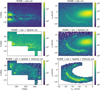 |
Fig. C.1 preselection sample using Gaia EDR3. The same criteria is applied as in Fig. 2 for comparison. See text for more details. |
References
- Alves, J., Zucker, C., Goodman, A. A., et al. 2020, Nature, 578, 237 [NASA ADS] [CrossRef] [Google Scholar]
- Ambartsumian, V. A. 1947, The Evolution of Stars and Astrophysics (Izdatel’stvo Akad Nauk Arm SSR, Erevan) [Google Scholar]
- Ambartsumian, V. A. 1949, Astron. Z., 26, 3 [NASA ADS] [Google Scholar]
- Andrae, R., Fouesneau, M., Creevey, O., et al. 2018, A&A, 616, A8 [NASA ADS] [CrossRef] [EDP Sciences] [Google Scholar]
- Bailer-Jones, C. A. L. 2015, PASP, 127, 994 [Google Scholar]
- Bastian, N., Covey, K. R., & Meyer, M. R. 2010, ARA&A, 48, 339 [Google Scholar]
- Blaauw, A. 1946, Publ. Kapteyn Astron. Lab. Groningen, 52, 1 [NASA ADS] [Google Scholar]
- Blaauw, A. 1964a, ARA&A, 2, 213 [Google Scholar]
- Blaauw, A. 1964b, The Scorpio-Centaurus Association, 20 (Cambridge University Press), 50 [Google Scholar]
- Blaauw, A. 1991, The Physics of Star Formation and Early Stellar Evolution, 342 [Google Scholar]
- Bobylev, V. V. 2015, Astrophysics, 57, 583 [NASA ADS] [Google Scholar]
- Bobylev, V. V., & Bajkova, A. T. 2014, Astron. Lett., 40, 783 [NASA ADS] [CrossRef] [Google Scholar]
- Bossini, D., Vallenari, A., Bragaglia, A., et al. 2019, A&A, 623, A108 [NASA ADS] [CrossRef] [EDP Sciences] [Google Scholar]
- Bouy, H., & Alves, J. 2015, A&A, 584, A26 [NASA ADS] [CrossRef] [EDP Sciences] [Google Scholar]
- Brandt, T. D. 2018, ApJS, 239, 31 [Google Scholar]
- Bressan, A., Marigo, P., Girardi, L., et al. 2012, MNRAS, 427, 127 [NASA ADS] [CrossRef] [Google Scholar]
- Chabrier, G. 2001, ApJ, 554, 1274 [NASA ADS] [CrossRef] [Google Scholar]
- Chen, Y., Girardi, L., Bressan, A., et al. 2014, MNRAS, 444, 2525 [Google Scholar]
- Chen, Y., Bressan, A., Girardi, L., et al. 2015, MNRAS, 452, 1068 [Google Scholar]
- Chen, Y., Girardi, L., Fu, X., et al. 2019, A&A, 632, A105 [EDP Sciences] [Google Scholar]
- Damiani, F., Prisinzano, L., Pillitteri, I., Micela, G., & Sciortino, S. 2019, A&A, 623, A112 [NASA ADS] [CrossRef] [EDP Sciences] [Google Scholar]
- de Bruijne, J. H. J. 1999, MNRAS, 310, 585 [NASA ADS] [CrossRef] [Google Scholar]
- de Geus, E. J. 1992, A&A, 262, 258 [NASA ADS] [Google Scholar]
- de Zeeuw, P. T., Hoogerwerf, R., de Bruijne, J. H. J., Brown, A. G. A., & Blaauw, A. 1999, AJ, 117, 354 [Google Scholar]
- Elias, F., Alfaro, E. J., & Cabrera-Caño, J. 2009, MNRAS, 397, 2 [CrossRef] [Google Scholar]
- Evans, D. W., Riello, M., De Angeli, F., et al. 2018, A&A, 616, A4 [NASA ADS] [CrossRef] [EDP Sciences] [Google Scholar]
- Feiden, G. A. 2016, A&A, 593, A99 [NASA ADS] [CrossRef] [EDP Sciences] [Google Scholar]
- Finkbeiner, D. P. 2003, ApJS, 146, 407 [Google Scholar]
- Gagné, J., Faherty, J. K., & Mamajek, E. E. 2018a, ApJ, 865, 136 [Google Scholar]
- Gagné, J., Mamajek, E. E., Malo, L., et al. 2018b, ApJ, 856, 23 [Google Scholar]
- Gaia Collaboration 2016a, A&A, 595, A1 [NASA ADS] [CrossRef] [EDP Sciences] [Google Scholar]
- Gaia Collaboration (Brown, A. G. A., et al.) 2016b, A&A, 595, A2 [NASA ADS] [CrossRef] [EDP Sciences] [Google Scholar]
- Gaia Collaboration (Brown, A. G. A., et al.) 2018, A&A, 616, A1 [NASA ADS] [CrossRef] [EDP Sciences] [Google Scholar]
- Gaia Collaboration (Brown, A. G. A., et al.) 2021, A&A, 649, A1 [NASA ADS] [CrossRef] [EDP Sciences] [Google Scholar]
- Galli, P. A. B., Joncour, I., & Moraux, E. 2018, MNRAS, 477, L50 [Google Scholar]
- Goldman, B., Röser, S., Schilbach, E., Moór, A. C., & Henning, T. 2018, ApJ, 868, 32 [Google Scholar]
- Gould, B. A. 1879, Resultados del Observatorio Nacional Argentino, 1 [Google Scholar]
- Guo, D. 2022, PhD thesis, University of Amsterdam, Anton Pannekoek Institute for Astronomy, The Netherlands [Google Scholar]
- Guo, D., de Koter, A., Kaper, L., Brown, A. G. A., & de Bruijne, J. H. J. 2021, A&A, 655, A45 [NASA ADS] [CrossRef] [EDP Sciences] [Google Scholar]
- Jilinski, E., Daflon, S., Cunha, K., & de la Reza, R. 2006, A&A, 448, 1001 [NASA ADS] [CrossRef] [EDP Sciences] [Google Scholar]
- Jordi, C., Gebran, M., Carrasco, J. M., et al. 2010, A&A, 523, A48 [NASA ADS] [CrossRef] [EDP Sciences] [Google Scholar]
- Jørgensen, B. R., & Lindegren, L. 2005, A&A, 436, 127 [Google Scholar]
- Kapteyn, J. C. 1914, ApJ, 40, 43 [NASA ADS] [CrossRef] [Google Scholar]
- Katz, D., Sartoretti, P., Cropper, M., et al. 2018, A&A, 622, A205 [Google Scholar]
- Kerr, R. M. P., Rizzuto, A. C., Kraus, A. L., & Offner, S. S. R. 2021, ApJ, 917, 23 [NASA ADS] [CrossRef] [Google Scholar]
- Kharchenko, N. V., Scholz, R. D., Piskunov, A. E., Röser, S., & Schilbach, E. 2007, AN, 328, 889 [NASA ADS] [Google Scholar]
- Kouwenhoven, M. B. N., Brown, A. G. A., Zwart, S. F. P., & Kaper, L. 2007, A&A, 474, 77 [NASA ADS] [CrossRef] [EDP Sciences] [Google Scholar]
- Krause, M. G. H., Burkert, A., Diehl, R., et al. 2018, A&A, 619, A120 [NASA ADS] [CrossRef] [EDP Sciences] [Google Scholar]
- Kroupa, P. 2001, MNRAS, 322, 231 [NASA ADS] [CrossRef] [Google Scholar]
- Lindegren, L., Madsen, S., & Dravins, D. 2000, A&A, 356, 1119 [NASA ADS] [Google Scholar]
- Lindegren, L., Hernández, J., Bombrun, A., et al. 2018, A&A, 616, A2 [NASA ADS] [CrossRef] [EDP Sciences] [Google Scholar]
- Luhman, K. L. 2020, AJ, 160, 186 [NASA ADS] [CrossRef] [Google Scholar]
- Luhman, K. L. 2022, AJ, 163, 24 [NASA ADS] [CrossRef] [Google Scholar]
- Luhman, K. L., & Esplin, T. L. 2020, AJ, 160, 44 [Google Scholar]
- Luhman, K. L., Herrmann, K. A., Mamajek, E. E., Esplin, T. L., & Pecaut, M. J. 2018, AJ, 156, 76 [Google Scholar]
- Luri, X., Brown, A. G. A., Sarro, L. M., et al. 2018, A&A, 616, A9 [NASA ADS] [CrossRef] [EDP Sciences] [Google Scholar]
- Maíz Apellániz, J., & Weiler, M. 2018, A&A, 619, A180 [Google Scholar]
- Mamajek, E. E., Pecaut, M. J., Nguyen, D. C., & Bubar, E. J. 2013, Protostars and Planets VI, Heidelberg, July 15–20, 2013, Poster #1K086 [Google Scholar]
- Marigo, P., Girardi, L., Bressan, A., et al. 2017, ApJ, 835, 77 [Google Scholar]
- Marrese, P. M., Marinoni, S., Fabrizio, M., & Altavilla, G. 2018, A&A, 621, A144 [Google Scholar]
- Nguyen, D. C., Mamajek, E., & Pecaut, M. 2013, Protostars and Planets VI, Heidelberg, July 15–20, 2013, Poster #1G024 [Google Scholar]
- Pannekoek, A. 1929, Publ. Astron. Inst. Univ. Amsterdam, 2, 71 [Google Scholar]
- Pastorelli, G., Marigo, P., Girardi, L., et al. 2019, MNRAS, 485, 5666 [Google Scholar]
- Pecaut, M. J., & Mamajek, E. E. 2013, ApJS, 208, 9 [Google Scholar]
- Pecaut, M. J., & Mamajek, E. E. 2016, MNRAS, 461, 794 [Google Scholar]
- Pecaut, M. J., Mamajek, E. E., & Bubar, E. J. 2012, ApJ, 746, 154 [Google Scholar]
- Perrot, C. A., & Grenier, I. A. 2003, A&A, 404, 519 [NASA ADS] [CrossRef] [EDP Sciences] [Google Scholar]
- Perryman, M. A. C., European Space Agency., & FAST Consortium 1997, The Hipparcos and Tycho catalogues astrometric and photometric star catalogues derived from the ESA Hipparcos Space Astrometry Mission (ESA Publications Division) [Google Scholar]
- Preibisch, T. & Zinnecker, H. 2007, Proceedings of the International Astronomical Union 2, IAU Symposium 237, 270 [Google Scholar]
- Preibisch, T., & Mamajek, E. 2008, Handbook of Star Forming Regions, 5 [Google Scholar]
- Ratzenböck, S., Großschedl, J. E., Alves, J., et al. 2023a, A&A, 678, A71 [NASA ADS] [CrossRef] [EDP Sciences] [Google Scholar]
- Ratzenböck, S., Großschedl, J. E., Möller, T., et al. 2023b, A&A, 677, A59 [NASA ADS] [CrossRef] [EDP Sciences] [Google Scholar]
- Reid, M. J., Menten, K. M., Brunthaler, A., et al. 2014, ApJ, 783, 130 [Google Scholar]
- Rizzuto, A. C., Ireland, M. J., & Robertson, J. G. 2011, MNRAS, 416, 3108 [Google Scholar]
- Rizzuto, A. C., Ireland, M. J., & Kraus, A. L. 2015, MNRAS, 448, 2737 [NASA ADS] [CrossRef] [Google Scholar]
- Röser, S., Schilbach, E., Goldman, B., et al. 2018, A&A, 614, A81 [NASA ADS] [CrossRef] [EDP Sciences] [Google Scholar]
- Salpeter, E. E. 1955, ApJ, 121, 161 [Google Scholar]
- Sullivan, K., & Kraus, A. L. 2021, ApJ, 912, 137 [NASA ADS] [CrossRef] [Google Scholar]
- Tang, J., Bressan, A., Rosenfield, P., et al. 2014, MNRAS, 445, 4287 [NASA ADS] [CrossRef] [Google Scholar]
- van Leeuwen, F. 2007, Astrophysics and Space Science Library, 350, Hipparcos, the New Reduction of the Raw Data, ed. F. van Leeuwen (Dordrecht: Springer Netherlands) [CrossRef] [Google Scholar]
- Vos, D. A. I., Cox, N. L. J., Kaper, L., Spaans, M., & Ehrenfreund, P. 2011, A&A, 533, A129 [NASA ADS] [CrossRef] [EDP Sciences] [Google Scholar]
- Wright, N. J., & Mamajek, E. E. 2018, MNRAS, 476, 381 [Google Scholar]
- Zari, E., Hashemi, H., Brown, A. G. A., Jardine, K., & de Zeeuw, P. T. 2018, A&A, 620, A172 [NASA ADS] [CrossRef] [EDP Sciences] [Google Scholar]
But see Ratzenböck et al. (2023a) for a more detailed discussion of the star formation history of the Sco-Cen region.
After the submission of this paper, new analyses of the Sco-Cen region based on Gaia (E)DR3 data have appeared in literature (Luhman 2022; Ratzenböck et al. 2023b, a) with more detailed information on the clustering, membership and star formation history. Although the results in the current paper are based on DR2 data and explore a different strategy, the results agree well, broadening the base for our understanding of the census of Sco OB2. In Ratzenböck et al. (2023b), a thorough discussion is presented comparing their results with those presented in earlier studies.
https://www.cosmos.esa.int/web/gaia/dr2-known-issues; alternatively, the reader can now directly download RUWE as a separate table from the Gaia Archive.
See also Fig. 13 in Ratzenböck et al. (2023b).
Ratzenböck et al. (2023b) arrive at a final membership sample of about 13 000 co-moving objects based on DR3 data, exploring a larger area on the sky than in this analysis.
The superscript ⊤ marks the transpose operation on a vector or a matrix. All vectors in this work are defined as column vectors by default in order to keep the notations consistent with matrix multiplication rules.
Further information about the algorithm and clustering methods in general can be found in https://scikit-learn.org/stable/modules/clustering.html
With their respective cluster search algorithms Kerr et al. (2021) and Ratzenböck et al. (2023b) identify more subgroups; Ratzenböck et al. (2023b) arrive at 37 subgroups divided over 7 areas, of which Pipe, CrA, Cham and NE are largely outside the field that we have explored in this paper. The derived properties of our subgroups are largely in line with those found by Ratzenböck et al. (2023b) in US, UCL, and LCC.
Download from http://stev.oapd.inaf.it/cgi-bin/cmd
Ratzenböck et al. (2023a) present a detailed analysis of the star formation history of the Sco-Cen association. Grosso modo, they arrive at a similar, though much more detailed spatial age map of this region.
All Tables
All Figures
|
Fig. 1 Sco OB2 census by de Zeeuw et al. (1999) in Galactic coordinates. The white triangles mark the 521 identified HIPPARCOS members. The boundaries of the three subgroups are indicated by the dashed white lines: from left to right, Upper Sco (US), Upper Centaurus Lupus (UCL), and Lower Centaurus Crux (LCC) appear, respectively. The “new” subgroup Lower Sco is indicated by a dashed white circle; the position of the open cluster IC 2602 is displayed by a white diamond. The Ophiuchus star forming region is centered at the small white circle (l = 354°, b = 17°). The background image is taken from the Hα map of Finkbeiner (2003). |
| In the text | |
|
Fig. 2 Different stages applied to preselect the data. Left column: stellar density maps in the l-b plane; Right column: stellar density maps in the transverse velocity plane. The color bars show the color coding of point-source density in log-scale. Row 1: all the candidates downloaded from the Gaia Archive. Row 2: after applying the filter of RUWE < 1.4 and (σϖ/ϖ) < 0.2. Row 3: in addition to the previous filters, apply all the conditions in the first table of Table 2. Row 4: in addition to the previous cuts, apply all the conditions in the second and third table in Table 2. This set contains the preselected candidates. |
| In the text | |
|
Fig. 3 Result of membership selection. The members are represented by the points color coded according to membership probability from 0.95 to ~0.98 (black to orange). The brighter the color, the higher the probability. The nonmembers are colored gray. Left panel: members and nonmembers plotted in proper motion space (equatorial coordinates). Middle panel: members and nonmembers plotted in parallax – total proper motion space. The inset shows a histogram of membership probability. Right panel: smoothed parallax distribution of the members. The horizontal axis shows the number density, while the vertical axis displays the parallax. |
| In the text | |
|
Fig. 4 Sky map presenting the members of Sco OB2 based on our analysis. Upper panel: the distance (1000/ϖ) of the members against Galactic longitude l. Lower panel: members shown in the Galactic coordinate plane. The subgroup boundaries in de Zeeuw et al. (1999) are marked by the black dashed lines. In both panels, the membership probability is color coded as represented by the color bar. The open cluster IC 2602 is shown as a black diamond; according to our analysis, it is not part of Sco OB2. |
| In the text | |
|
Fig. 5 Subgroups identified by DBSCAN in Galactic coordinates. The upper panel shows distance against Galactic longitude, the lower panel displays the Galactic latitude against longitude. The members of the subgroups are plotted in various colors (see in-set legend), and the members that do not belong to any subgroup (Halo stars) are colored gray. |
| In the text | |
|
Fig. 6 Subgroups identified by DBSCAN in cartesian coordinates. The subgroup color code is the same as in Fig. 5. The black dots mark the mean position of the subgroups. The Sun’s position, in this case also the origin, is indicated with the usual (orange) symbol ⊙. |
| In the text | |
|
Fig. 7 Three dimensional view demonstrating the spatial structure formed by the subgroups. |
| In the text | |
|
Fig. 8 Proper motion vector point diagrams in both Galactic (left panel) and ICRS coordinates (right panel). The subgroups are colored the same as Fig. 5. |
| In the text | |
|
Fig. 9 Position and proper motion of the members in Galactic coordinates. The median proper motion across all members is ~30 mas yr−1, with a standard deviation of ~5.6 mas yr−1. The black arrows are the reflex of solar motion observed at parallax 7 mas on a grid of coordinate points. The solar velocity in the local standard of rest (U, V, W) = (9.6, 14.6, 9.3) km s−1 is taken from the local standard of rest in Reid et al. (2014). |
| In the text | |
|
Fig. 10 Tangential velocity distribution of Sco OB2 in vα*-vδ space. All panels contain the same contours representing the number density of all candidates after preselection. Panel a: stellar density map of all candidates in the tangential velocity space. The darker the color, the higher the density. The high density area forms a curved shape. Panel b: plot of the members where all the subgroups are colored differently. The members overlap with the high density area. The subgroups together form a continuous distribution in the tangential velocity space, thus there is no incentive to separate Sco OB2 into subgroups based on transverse velocity distinctions. The mean error bar is indicated with a black cross. The size of the mean error is ~0.3 km s−1 for both dimensions. Panel c: plot of the group model velocities, well overlapping with the high density area. The model shows that the velocity of Sco OB2 can be described as one continuous velocity field instead of multiple subgroups with distinct velocities. Panel d: plot of the field model velocities. It does not directly cover the nonmembers in this diagram, but with the help of a very large velocity dispersion (~20–100 km s−1) it is adequate to represent the nonmembers. |
| In the text | |
|
Fig. 11 Radial velocity vrad (km s−1) plotted as a function of Galactic longitude l (deg). The panels a, b, c, and d show the radial velocity of a subset of the stellar content as in Fig. 10, but in a different parameter space. The vertical axis of the plots is cropped down to (−50, 50) km s−1, while there are a few sources whose radial velocity can reach over 100 km s−1. Within our members, only one star in US exceeds this limit at ~70 km s−1. Panel a: plot of all preselected candidates with the contours showing the density. The brighter the color, the higher the density. The high density area follows a linear relation. Panel b: the radial velocity (with error bars) of the members. The subgroups are colored as in Fig. 5. The members overlap with the high density area except for a few outliers. All subgroups together form a continuous distribution, proving again that there is no incentive to separate Sco OB2 into subgroups based on a kinematical distinction. We note that most outliers are from the Halo population (gray points with error bars). Panel c: plot of the projected group model. The model points in this space are colored the same as their corresponding subgroups. The model overlays the high density area, but has a slight shift in radial velocity relative to the observations. The shift reflects the fact that our model does not use radial velocity to constrain the optimization process. Panel d: plot of the field model (red points). It separates from the high density zone just enough to generate the group-field model contrast. |
| In the text | |
|
Fig. 12 The radial-velocity dispersion per subgroup in Sco OB2. Panel a: radial velocity vrad (km s−1) plotted as a function of Galactic longitude l (deg). All the candidates with a radial velocity measurement are colored gray; all the members with black error bars. The projected group model is in blue, and the field model in red. The radial velocity range of the plots is limited to (−50, 50) km s−1, while a few candidates exceed this limit. Panel b: the histograms of observed radial velocity per subgroup. The radial velocity dispersion of Sco OB2 is inflated by the projection effect, where the majority of the radial velocities are distributed within range (−10, 20) km s−1. Panel c: radial-velocity dispersion per subgroup. The radial velocity predicted by the kinematic model has been subtracted from the measured velocity. Panel d: the radial-velocity dispersion per subgroup, smoothed with measurement errors. The peak position is marked by a vertical line, and the peak value is listed in the legend. |
| In the text | |
|
Fig. 13 Difference between the observed and model velocity vectors by the amplitude of vectorial difference (top panel) and angular difference (bottom panel). |
| In the text | |
|
Fig. 14 Three dimensional vector field map, in Galactic cartesian coordinates, of the 616 members with a radial velocity in Gaia DR2. The members of the subgroups are colored (see inset). The black arrow shows the median motion of all members. The sources highlighted by red circles and arrows have ΔV ≥ 0.75 and orange diamonds have cos(vobs, vp) ≤ 0.8, and are potential interlopers. Most of them meet both conditions except four. |
| In the text | |
|
Fig. 15 Relative proper motion vectors in Sco OB2. The vectors are obtained by subtracting the predicted proper motion of the continuous velocity model from the observed proper motion. The direction of motion of the vector is color-coded as shown in the color wheel. Zero degrees is defined as pointing to the left of the plot, as the x-axis is flipped, and 90 degree pointing to the positive end of the y-axis. The median location of the subgroups is marked by a black circle with the subgroup name. |
| In the text | |
|
Fig. 16 Median angle map based on Fig. 15. Each pixel is color-coded by the median angle of the vectors within 2.5 degrees. A minimum of 20 stars is required to produce a colored pixel. The color code of the angle is the same as in Fig. 15. |
| In the text | |
|
Fig. 17 BP/RP excess filter applied to the members. Left panel: the C−(GBP − GRP) relation. The majority of stars in Sco OB2 are below the fitted curve, thus the filter C < 1.22 + 0.04(GBP − GRP)2 selects the stars with good color quality, painted in blue. The stars excluded by the filter are colored in gray. Right panel: the color-magnitude diagram after filtering. The stars that passed the filter are plotted in blue, those excluded in gray. The black dashed line indicates the zero age main sequence (ZAMS) from the PARSEC model. |
| In the text | |
|
Fig. 18 Interstellar extinction as listed in Gaia DR2. Upper panel: bimodal distribution of the extinction in the sight lines toward Sco OB2 (AG versus (GBP − GRP)). The blue branch and red branch are produced by a cut at (GBP − GRP) = 1 mag. Lower panel: histogram of AG of the blue and red branch populations. |
| In the text | |
|
Fig. 19 Results of the bootstrap method to estimate the errors on age and extinction, per subgroup. Each circle centers on an age-extinction combination that occurs at least once in the 200 redrawn samples. The size of the circle is proportional to the number of occurrences. The biggest circle represents the most frequent age-extinction combination, and is marked with the highest occurrence number. The higher the number, the more yellow the circle. The inset lists the name of the subgroup, the number of stars, the median age and extinction, and the uncertainty. |
| In the text | |
|
Fig. 20 Best fit isochrone per subgroup (black line) with the zero-age main sequence (ZAMS, dashed gray line) for reference. Only US and LS are significantly younger than the on average 17.5 Myr old population of Sco OB2. We note the in total four white dwarfs in the bottom left corner in the CMD of the Halo population and UCL-2; these are most likely interlopers. |
| In the text | |
|
Fig. 21 Color-magnitude diagram showing the empirical isochrone produced by a running mean (black line), and offset isochrones defined in units of the running standard deviation (dashed line). The members brighter than the running mean (negative offset) are colored blue, the ones fainter (positive offset) colored red, and those close to the mean (near zero offset) colored yellow. |
| In the text | |
|
Fig. 22 Relative age map in Galactic coordinates. The color code corresponds to the median offset value within a 4° radius per pixel. The median position of the subgroup is indicated by a black circle labeled by name. The top panel is based on all members; the middle panel with only the members with (GBP − GRP) > 1 mag (mostly PMS stars); the lower panel with only the members with (GBP − GRP) < 1 mag (mostly MS stars). We find a strong correspondence with the result by Pecaut & Mamajek (2016). |
| In the text | |
|
Fig. 23 Relative age map in cartesian coordinates. The color code corresponds to the median offset value within a 10 pc radius per pixel. The median position of the subgroup is indicated by a black circle labeled by name. The orange symbol ⊙ indicates the location of the Sun. The panels in the top, middle, and bottom rows show the views in X–Y, Y–Z, and X–Z space, respectively. The left diagrams are produced with all members; the middle ones with only the members with (GBP − GRP) > 1 mag (mostly PMS stars); and the right ones with only the members with (GBP − GRP) < 1 mag (mostly MS stars). |
| In the text | |
|
Fig. 24 Membership probability distribution of the members in Z99 (red) and R11 (green) in common with our preselected samples. The bin width in this plot is 0.05. |
| In the text | |
|
Fig. 25 Potential interlopers due to deviating radial velocity plotted in the color-magnitude diagram. The blue points show all the members of Sco OB2 that pass the BP/RP excess filter; the orange points are the members with radial velocity in Gaia DR2; the red circles mark the potential interlopers discussed in Sect. 5.2. For reference, the ZAMS model is included as a black dashed line. The data points are not corrected for extinction and reddening. |
| In the text | |
|
Fig. C.1 preselection sample using Gaia EDR3. The same criteria is applied as in Fig. 2 for comparison. See text for more details. |
| In the text | |
Current usage metrics show cumulative count of Article Views (full-text article views including HTML views, PDF and ePub downloads, according to the available data) and Abstracts Views on Vision4Press platform.
Data correspond to usage on the plateform after 2015. The current usage metrics is available 48-96 hours after online publication and is updated daily on week days.
Initial download of the metrics may take a while.