| Issue |
A&A
Volume 695, March 2025
|
|
|---|---|---|
| Article Number | A74 | |
| Number of page(s) | 20 | |
| Section | Planets, planetary systems, and small bodies | |
| DOI | https://doi.org/10.1051/0004-6361/202453011 | |
| Published online | 11 March 2025 | |
A novel method for estimating the far-ultraviolet flux, and a catalogue for disc-hosting stars in nearby star-forming regions
1
Dipartimento di Fisica, Università degli Studi di Milano,
Via Celoria 16,
20133
Milano, Italy
2
Université Côte d’Azur, Observatoire de la Côte d’Azur, CNRS, Laboratoire Lagrange,
06300
Nice, France
3
European Southern Observatory,
Karl-Schwarzschild-Str. 2,
85748
Garching bei München, Germany
4
Dipartimento di Fisica e Astronomia, Università di Firenze,
Via G. Sansone 1,
50019,
Sesto F.no (Firenze), Italy
5
Department of Astrophysics, University of Vienna,
Türkenschanzstrasse 17,
1180
Vienna, Austria
6
Dipartimento di Fisica e Astronomia, Università di Bologna, Via Gobetti 93/2, 40122, Bologna, Italy; INAF – Osservatorio Astrofisico di Arcetri, Largo E. Fermi 5,
50125
Firenze,
Italy
★ Corresponding author; rossella.anania@unimi.it
Received:
15
November
2024
Accepted:
27
January
2025
When protoplanetary discs are externally irradiated by far-ultraviolet (FUV) photons from OBA-type stars, they lose material through photoevaporative winds. This reduces the amount of material that is available to form planets. Understanding the link between the environmental irradiation and the observed disc properties requires accurately evaluating the FUV flux at disc-hosting stars, which can be challenging because of the uncertainty in stellar parallax. We addressed this issue by proposing a novel approach: using the local density distribution of a star-forming region (i.e. 2D pairwise star separation distribution) and assuming isotropy, we inferred the 3D separation between disc-hosting stars and massive stars. We tested this approach on synthetic clusters and showed that it significantly improves accuracy compared to previous methods. We computed the FUV fluxes for numerous star-bearing discs in seven regions within ~200 pc, six regions in Orion and in Serpens sub-regions. We provided a publicly accessible catalogue. We found that discs in regions hosting late-type B and early-type A stars can reach non-negligible FUV radiation levels for the disc evolution (10–100 G0). We investigated dust disc masses relative to FUV fluxes and detected indications of a negative correlation when we restricted the investigation to average region ages. However, we emphasize the need for more stellar and disc measurements at >102 G0 to probe the dependence of disc properties on environmental irradiation. The method presented in this work is a powerful tool that can be expanded to additional regions.
Key words: accretion, accretion disks / catalogs / protoplanetary disks / stars: distances / stars: protostars
© The Authors 2025
 Open Access article, published by EDP Sciences, under the terms of the Creative Commons Attribution License (https://creativecommons.org/licenses/by/4.0), which permits unrestricted use, distribution, and reproduction in any medium, provided the original work is properly cited.
This article is published in open access under the Subscribe to Open model. Subscribe to A&A to support open access publication.
1 Introduction
The majority of young stars (and their surrounding protoplanetary disc) forms in dense and massive clusters or associations (e.g. Miller & Scalo 1978; Lada et al. 2010), where the ultraviolet (UV) radiation emitted by massive stars of primarily spectral types O and B can strongly influence the disc evolution and planet formation, as well as their physical and chemical composition. Vioque et al. (2023) showed that massive star-forming regions become less clustered over time and that no preferential position is occupied by massive stars in the cluster. Therefore, as protoplanetary discs that are initially distant from massive stars may still experience intense irradiation over time, it is essential to be aware of the distribution and characteristics of massive stars in star-forming regions in which these discs are observed.
The intense extreme-ultraviolet (EUV) and far-ultraviolet (FUV) radiation from OB stars heats the outermost disc regions, which are weakly gravitationally bound to the central star. This leads to an outside-in depletion of material. This process is known as external photoevaporation and can result in smaller, less massive, and shorter-lived discs (see Winter & Haworth 2022 for a review, and references therein). The dust component, depending on its size and composition, can also be affected by photoevaporation, with dust grains being trapped in thermal winds and carried away from the disc (e.g. Facchini et al. 2016; Sellek et al. 2020a). Disc truncation due to photoevaporation prevents the disc from spreading viscously, and the loss of gas and dust reduces the location and material available for forming new planets (Sellek et al. 2020b; Qiao et al. 2023). As grain growth and the formation of gas giants in the outermost disc regions can be limited by photoevaporation, this will result in a different observed exoplanet population (e.g. Ndugu et al. 2018).
Evidence of external photoevaporation in action on protoplanetary discs is probed by direct observations of proplyds, which are protoplanetary discs seen in optical lines as ionised gas clouds with a characteristic comet-like shape, with the cusp pointing toward the nearest massive star (e.g. O’Dell et al. 1993; Otter et al. 2021; Berné et al. 2024; Aru et al. 2024). These fascinating objects are found in highly irradiated environments (≳3 × 10³G01; Kim et al. 2016) in close proximity to massive O-type or early-type B stars (within ~0.1 pc). However, proplyds are only representative of the most extreme environmental conditions, while the majority of discs forms and evolves in moderately irradiated environments (102–103 G0 , Fatuzzo & Adams 2008), where external irradiation is driven by less massive stars, and the peculiar proplyd-like shape is not detectable. In intermediate irradiated environments, the effect of photoevaporation is indirectly suggested by the dependence of the (sub-)millimeter continuum flux emission on the distance from the most massive star, such as in σ Orionis (Ansdell et al. 2017; Maucó et al. 2023) and λ Orionis (Ansdell et al. 2020). The low-irradiation extended population of Orion investigated by the SODA Survey (∼1–100 G0) also showed a correlation between (sub-)millimeter continuum flux emission and FUV flux (van Terwisga & Hacar 2023). Moreover, a weak correlation between the gas and dust disc sizes and the FUV flux was even found for the AGE-PRO sample in the Upper Scorpius region (2–12 G0; Anania et al. 2025), where adding external photoevaporation to a viscous model resulted in a better reproduction of the gas disc sizes.
Depending on the strength and intensity of the incident UV photons, the thermal and chemical structure of protoplanetary discs can also be altered, in particular, in the most external surface layers (Walsh et al. 2013), while recent results from the eXtreme UV Environments (XUE) James Webb Space Telescope (JWST) program showed that the chemistry of the inner disc (<10 au) is similar in lower and higher irradiated discs (Ramírez-Tannus et al. 2023). Astrochemical models predict that the molecular composition of the outer disc is probably influenced by external irradiation (e.g. Nguyen et al. 2002; Walsh et al. 2013, 2014). The impact of intense UV fields on the molecular composition of the outermost disc regions is supported by observational evidence of highly UV-irradiated discs (e.g.  detection in a ∼105 G0 irradiated disc Berné et al. 2023). However, at moderate and typical UV levels (<103 G0), no direct detection is currently reported.
All the above results highlight that the environment plays a crucial role in shaping the physical and chemical properties of the disc even at moderate levels of irradiation. Therefore, it is essential to accurately quantify the FUV flux at the position of disc-hosting stars to reliably compare the predictions of disc evolution models and astrochemical models with observational outcomes, and to investigate the role of the environmental FUV irradiation on the disc and planetary evolution. However, it can be very hard to evaluate the FUV flux because it requires knowledge of the distribution of stars in a three-dimensional (3D) space, which is highly influenced by parallax uncertainties. The separation value typically used in flux calculations is the 2D separation projected on the sky plane, assuming an average distance to the entire cluster. This precludes an estimate of the uncertainty on the distance between stars, and therefore, on the FUV flux to which a given protoplanetary disc is exposed.
Pabst et al. (2022) provided an FUV flux map of the Orion region by estimating the stellar luminosity under the assumption that it is entirely reradiated in the dust continuum as observed in infrared wavelengths. The FUV flux was calculated applying an approximately constant ratio of the FUV luminosity and stellar luminosity for early OB-type stars, and in this case, also using 2D projected separation distances from the most massive stars. Moreover, late-type B and early-type A stars, which are usually neglected in the FUV flux calculation, can significantly influence the evolution of protoplanetary discs when they are located close to them.
We aim to provide a more precise estimate of the FUV flux, along with its uncertainty, at the position of disc-hosting stars in nearby star-forming regions. Specifically, we propose using the available information on the 2D geometry of a star-forming region to constrain the 3D separation between massive stars and disc-hosting stars, which is the largest source of uncertainty in the flux calculation. We provide a publicly available catalogue of the FUV flux experienced by disc-hosting stars located in nearby regions presenting previous studies of disc populations (see Table B.1), covering regions within ∼200 pc that have been well-investigated by protoplanetary disc surveys (i.e. Taurus and Lupus), well-known Orion star-forming regions (i.e. ONC and λOrionis), and Serpens sub-regions at an average distance of ∼500 pc. The selected disc sample and the star-forming regions are discussed in Sect. 2. In Sect. 3, we describe the selection criteria for the irradiating massive stars. In Sect. 4, we introduce three approaches to evaluating the FUV flux accounting for the uncertainty in line-of-sight distance, and we test the methods on synthetic clusters in Sect. 4.4. The results for the various star-forming regions are presented in Sect. 5, along with an investigation of the relation between external UV radiation and measured dust disc masses in Sect. 5.3. In Sect. 6, we discuss the results we obtained and the uncertainties and future improvement of the method. We conclude in Sect. 7. The Table with the FUV flux estimate at the position of numerous discs in the regions studied, is available at the CDS.
2 Target regions and discs
We evaluated the FUV flux at the position of disc-hosting stars located in nearby star-forming regions with distance ranges from Taurus (∼140 pc) to Serpens (∼500 pc). In order to explore the level of FUV irradiation experienced by discs in various environmental conditions, we included regions hosting a different number of massive stars covering a wide range of spectral types and featuring well-known populations of disc-bearing stars with estimated ages ≲10 Myr. Our investigations of the regions are thus motivated by previous studies of disc populations. The rationale for this selection was to present and apply our method for calculating the FUV flux and its associated uncertainty. By doing so, we access irradiation on individual discs and statistically investigate different regions. In particular, we selected discs from seven of the most nearby star-forming regions that have been intensively investigated by disc surveys (Manara et al. 2023 and references therein). These are Upper Scorpius (Upper Sco), Lupus, Taurus, ρ Ophiuchi (ρ Oph), Chamaeleon I (ChamI), Chamaeleon II (ChamII), and Corona Australis (CrA). In addition, we included discs from six star-forming regions in Orion, which are the Orion nebula cluster (ONC), σ Orionis (σ Ori), λ Orionis (λ Ori), 25 Orionis (25 Ori), NGC 2024, and NGC 1977, where more luminous O-type and early B-type stars are located. Furthermore, the Serpens region was divided into four disc clusters based on Anderson et al. (2022).
The number of discs considered in each region and the references for the selected disc sample are listed in Table 1. In particular, we refer to Manara et al. (2023) for the disc sample in the most nearby regions (≲200 pc) and to Anderson et al. (2022) for the ClassII Serpens discs. The discs in the Orion region were taken from various catalogues (see Table 1). Specifically, the disc sample in the 25 Ori region consists of the sources in Briceño et al. (2019), who presented counterparts in the AllWISE catalogue (Cutri et al. 2021) and infrared excess according to Luhman (2022a), which is consistent with the classification of full, transitional, or evolved discs (Esplin et al. 2018). For the ONC, we selected the discs located in the innermost region around the Trapezium cluster, as included by Eisner et al. (2018), and we completed this initial catalogue with the proplyds listed in the catalogue by Ricci et al. (2008). Future investigations will expand this initial catalogue to include discs that are located in the outermost part of the region.
Star-forming regions and corresponding disc samples.
3 FUV flux calculation: Massive hot stars and their properties
The total FUV flux in a certain position is usually computed by adding the contribution of individual neighbouring massive stars,
 (1)
where LFUV,m is the FUV luminosity of the massive star, and |xdisc − xm | is the separation between the location at which we wish to evaluate the flux (in our case, the disc position) and the massive star. In the calculation of the FUV flux, the selected massive stars are often limited to the nearest (or a few nearest) massive stars in the field, assuming that the closest stars dominate the flux, while the influence of more distant stars is typically neglected. However, including high-and intermediatemass stars that are not members of a specific star-forming region increases the completeness of the analysis. In our study, we used a large sample of massive stars, which enabled us to explore the impact of irradiation on discs in regions with fewer massive stars. The criteria we employed to select the massive stars that contribute to the overall FUV flux on individual discs are discussed in Sect. 3.1, and Sect. 3.2 describes how we retrieved the FUV luminosity.
(1)
where LFUV,m is the FUV luminosity of the massive star, and |xdisc − xm | is the separation between the location at which we wish to evaluate the flux (in our case, the disc position) and the massive star. In the calculation of the FUV flux, the selected massive stars are often limited to the nearest (or a few nearest) massive stars in the field, assuming that the closest stars dominate the flux, while the influence of more distant stars is typically neglected. However, including high-and intermediatemass stars that are not members of a specific star-forming region increases the completeness of the analysis. In our study, we used a large sample of massive stars, which enabled us to explore the impact of irradiation on discs in regions with fewer massive stars. The criteria we employed to select the massive stars that contribute to the overall FUV flux on individual discs are discussed in Sect. 3.1, and Sect. 3.2 describes how we retrieved the FUV luminosity.
3.1 Selection of massive stars
In order to perform a nearly comprehensive selection of massive stars that influence the total FUV flux on discs in specific regions, we cross-matched multiple stellar catalogues as described below.
ALS III catalogue: We selected from the ALS III catalogue (Pantaleoni-Gonzalez et al., in prep.) all the massive stars within 2 kpc of the Sun with good Gaia DR3 (Gaia Collaboration 2023)2 photometric and spectrometric measurements3. This first selection provided a pure list of the known confirmed most massive stars with accurate Gaia measurements. It includes 5791 stars covering spectral type O, B2, and earlier for main-sequence stars, B5 and earlier for giants, B9 and earlier for super-giants, Wolf-Rayet (WR) stars, and stars lacking spectral type that were classified as massive since they are situated above the 20 kK extinction track in the Hertzsprung–Russell (HR) diagrams.
Zari et al. (2021) catalogue: We cross-matched the initial ALSIII sample with the massive stars included in the catalogue of hot stars of Zari et al. (2021) that are located closer than 2 kpc to the Sun, and we added stars with effective temperatures greater than ∼8000 K (corresponding approximately to an A5V star) that were not included in our first sample. In total, we included 218 648 hot stars from this catalogue.
Gaia DR3 Extended Stellar Parametrizer for Hot Stars (ESP-HS) catalogue: We added the stars (if they were not already included in the previous catalogues) that are contained in the Gaia DR3 ESP-HS pipeline (Creevey et al. 2023; Fouesneau et al. 2023), which includes stars classified as A, B, and O based on the Extended Stellar Parametrizer for EmissionLine Stars classifier (ESP-ELS). This sample also includes stars that we excluded from the ALSIII initial selection due to their uncertainty or unknown parallax measurement, but that are classified as OBA-type. From this last sample, we excluded the outliers, which are stars whose effective temperature is associated with a higher parameter teff_esphs than 23 000 K, which present large error bars and are not reliable measurements.
HIPPARCOS catalogue: Because some of the most luminous stars are not included in the Gaia DR3 catalogue because the astrometric and photometric measurements are challenging, we included stars of type O, B, A0, and A1 that are contained in the HIPPARCOS catalogue (Perryman et al. 1997; van Leeuwen 2007)4 and were not included in the previous selection. The sample of massive stars selected from HIPPARCOS consists of ∼6000 stars.
SIMBAD database: For each star-forming region, we checked and included the stars without a temperature estimate in Gaia, but classified as O, B, A0, or A1 in SIMBAD with a well-defined luminosity class and reference.
It is particularly important to include not only the most luminous and massive stars in the FUV flux calculation, but also late B-type and early A-type stars in regions where no O-type and early B-type stars are found, but where the environmental irradiation field is not negligible (e.g. Upper Sco). While the average FUV flux is dominated by the most massive and luminous stars, late B-type and early A-type stars in the close proximity of protoplanetary discs might also be relevant in determining the FUV flux they experience, and consequently, in shaping the disc properties.
3.2 Calculation of the FUV luminosity
The FUV luminosity of the massive stars, which is a crucial parameter for evaluating the FUV flux, was evaluated employing the following procedure. We derived the effective temperature from the spectral type and luminosity class of the massive stars using the spectral classification given by the Galactic O-Star Catalogue (GOSC; Maíz Apellániz et al. 2017), when available. This classification is based on high-resolution spectra and not only on photometric measurements. For the stars without a GOSC spectral classification that are contained in the ESP-HS Gaia DR3 pipeline, we used the effective temperature addressed by the parameter teff_esphs and the associated uncertainty. This is a more reliable estimate of the effective temperature for OBA stars, which is performed by the ESP-HS package, and is characterised by the omission of the regions of the BP/RP and RVS spectra dominated by emission lines that influence the calculation of the temperature. Alternatively, we used the parameter teff_gspphot, which corresponds to a temperature based on the assumption that the entire spectrum has a temperaturebased origin in the stellar photosphere. The temperature of stars without these two parameters and the Hipparcos stars was retrieved from their spectral classification through tables referring to main-sequence stars, giant, super-giant, and WR stars (Pecaut & Mamajek 2013; Gray & Corbally 2009). After evaluating the effective temperature, we used the isochrones provided by the MIST models (Dotter 2016; Choi et al. 2016), assuming a fixed age (we used 1 Myr), to obtain the stellar parameters (stellar mass M⋆, radius R⋆, luminosity L⋆ , and the surface gravity g) needed to extract the stellar flux from the Castelli & Kurucz (2004) ATLAS9 stellar atmosphere models. Finally, the stellar flux was integrated in the FUV range of wavelengths [912–2400] Å to retrieve the FUV luminosity.
The method described above requires assuming an age for the massive stars because the stellar FUV luminosity increases during the stellar lifetime. However, Kunitomo et al. (2021) demonstrated that intermediate- and high-mass stars present a constant FUV luminosity after ∼1 Myr of evolution. Therefore, setting the stellar age to 1 Myr does not significantly influence the final result.
4 FUV flux calculation: Accounting for the uncertainty on the 3D separation
The FUV flux calculation is significantly influenced by the uncertainty on the true position of the stellar objects in 3D space. Even a small error on the relative separation between discs and massive stars can result in large uncertainties on the final flux values because the FUV flux strongly depends on the relative distance. This is particularly relevant the closer the discs are located to luminous stars, where errors on the relative distance between the two objects (caused by uncertainties in the parallax measurements) can be comparable to or exceed their separation. We addressed this issue by presenting and comparing three approaches to evaluate the FUV flux that take the uncertainty in the line-of-sight distance of the stars from the observer (measured from parallax) into account, which is known with a far lower precision than the RA and Dec components.
Method 1: Distance uncertainty sampling. The radial distance of each stellar object was evaluated by performing a Monte Carlo sampling of the distance distribution based on the Gaia DR3 and Hipparcos parallax measurements and uncertainties, as described in Sect. 4.1. In general, this method tends to underestimate FUV fluxes.
Method 2: 2D projected separation and distance uncertainty sampling. For close pairs of disc-massive star members of the same star-forming region, we evaluated the FUV flux using their (2D) projected separation, which resulted in a general overestimate of the actual flux. More details of this approach are provided in in Sect. 4.2.
Method 3: Local density function and distance uncertainty sampling. We assumed spatial isotropy throughout a starforming region, and we used the 2D geometry of the region to make arguments about the most probable 3D separation between stars. Specifically, we defined the probability of finding each pair of stars at a certain (3D) separation, given their (2D) projected distance on the sky plane, and we sampled from the corresponding cumulative distribution function to estimate the corresponding FUV flux, as detailed in Sect. 4.3. This approach provided our best estimate of the FUV flux and the associated uncertainty.
4.1 Method 1: Distance uncertainty sampling
To account for the uncertainty in the relative distance affecting the final FUV flux value, a standard approach involves using a Monte Carlo sampling of the distance distributions from Earth (or parallax values) of the single stars. This method is commonly used in nearby regions and where parallaxes are known with relative small uncertainties. The ALS III catalogue, as well as the catalogue of massive stars by Zari et al. (2021), provides the 50th, 16th, and 84th percentiles of the posterior distribution of distances. For the other stars contained in the Gaia catalogue, the median of the geometric distance posterior (Bailer-Joneset al. 2021), with 16th and 84th percentiles can be accessed and evaluated for the remnant stars. Larger uncertainties are registered in particular for faint objects, which are often embedded in gas clouds. This makes the detection more challenging (e.g. discs in the ρ Oph region). Larger uncertainties are also obtained for very luminous stars (e.g. σOri or θ1C). For objects without parallax measurements, we assigned parallax and parallax error as the median values of the nearest neighbour members of the same star-forming region with the same spectral type. The FUV flux at each disc position was evaluated by randomly assigning the radial distance of individual objects based on their provided distributions, and then repeating this process multiple times to determine the median, 16th, and 84th percentiles of the FUV flux. We show in Sects. 4.4 and 5 that this method in general tends to underestimate the FUV flux because the range of values that the 3D separation between objects can assume when randomly sampling from individual extended distributions of line-of-sight distances is large, and the probability of retrieving the correct separation is low. This method may yield unreliable FUV flux estimates when the distance uncertainties are comparable to or larger than the separation between an OBA star and the star that hosts the disc. In this scenario, even a small change in the relative separation between the disc and the massive star (due to large uncertainties in the line-of-sight position compared to the other two components on the sky plane) can lead to substantial variations in the final flux value.
4.2 Method 2: 2D projected separation and distance uncertainty sampling
The highest contribution to the FUV flux at the position of a certain disc-hosting star is given by massive star members of the same star-forming regions because they are closest to the object that is examined. However, the flux induced by these stars is subject toa large uncertainty due to the problem described above, where a small uncertainty in the line-of-sight position of two close objects can propagate into a large uncertainty in the FUV flux estimate. Therefore, for each star-forming region, we focused on these massive stars defined as members of the region. When we assume spatial isotropy within a given region, all directions have the same properties, meaning that stars with closer projected separations are more likely to be physically close (i.e. in 3D space). Hence, an upper limit of the FUV flux induced by massive star members of a certain region can be obtained considering the separation between them and the disc-hosting stars (members of the same region) projected on the sky plane at a line-of-sight distance corresponding to the object presenting the smallest distance uncertainty. For the massive stars outside the a certain region, we applied Method 1, described in the previous section, where an estimate of the uncertainty on the FUV flux is provided by randomly sampling the distribution of line- of-sight distances of single objects. While this approach offers an initial estimate of the flux when parallax measurements are not available, it has limitations. Specifically, as the primary source of the flux uncertainty for discs arises from the nearest massive stars, for which we only considered a 2D separation and ignored the errors (even when available) in the third dimension, we lose information about the accuracy of the flux calculation. The only source of the flux uncertainty in this method is produced by the separation between discs and the massive stars located outside their star-forming region, which is small because more distant stars influence the flux calculation less.
4.3 Method 3: Local density function and distance uncertainty sampling
For the massive stars and disc-hosting stars that are members of the same star-forming region, which can present errors on their 3D relative distance comparable to or larger than their 3D separation, we can improve Method 2 (Sect. 4.2). We can do this by appealing to the geometry of the region to find the best estimate of the 3D separation between stars given their 2D relative distance. We assumed that (i) the stellar members of a given starforming region have well-defined separations on the sky plane, meaning that we neglected errors in the RA and Dec positions, as these are minimal compared to the separations between stars and are smaller than the uncertainties in parallax, and (ii) spatial isotropy applies throughout the region. Considering a stellar member i, we employed the Bayes theorem to calculate the differential probability to find a second member j at a certain 3D separation rij, assuming to know the 2D separation Rij,
 (2)
(2)
In order to derive an analytic expression for Eq. (2) (i.e. likelihood and prior), we started by defining the differential probability to find a star j at a projected separation Rij from a star i in a small area dA = 2πRijdR,
 (3)
(3)
where  is the normalised probability density function of all the projected separations between the members of the star-forming region. Under the assumption of isotropy, the Abel theorem (Abel 1826) states that considering the (2D) surface density of neighbouring stars at distance R,
  , in the form
 (4)
(4)
the corresponding (3D) volume density,  , is uniquely defined as
 (5)
(5)
which is valid if  as r → ∞. As Abel’s inversion requires spherical symmetry to project a surface density in a volume density, we applied the theorem to the distribution of separations between pairs of stars in the isotropic case and to the separations from the centre of the region for a centrally concentrated region. Using Eq. (5), we rewrote Eq. (2) for a single pair of stars ij as
 (6)
(6)
which defines our probability distribution function (PDF), and where the factor multiplying the volume density was included to account for the geometrical effect when passing from 2D to 3D geometry. Using the precise RA and Dec measurements provided by Gaia DR3 and Hipparcos, we defined the separation R as the angular separation between two stars on the celestial sphere (evaluated using the Vincenty formula Vincenty 1975) projected to the median distance of the considered region. For each star-forming region, we used the membership census available in the literature (see Sect. 5 for references of the census) to evaluate  (hereafter
  ) as the distribution of the projected separations between pairs of stars in the same region. Subsequently, we estimated the 3D density profile
  (hereafter
  ) using Eq. (5), where r is the 3D (spherical) separation between stars. Finally, we sampled the probability distribution defined in Eq. (6) to derive the 3D separation between close stellar pairs, and we used this parameter to evaluate the FUV flux and the corresponding uncertainty.
When the geometry of the region was nearly centrally concentrated, we assumed spherical isotropy throughout the entire region and still used the expression in Eq. (6), but considering rij and Rij as the 3D and 2D separations from the centre of the distribution (i.e. rij is the radius of the sphere centred in the centre of the distribution, and Rij is radius in polar coordinates when neglecting the line-of-sight component). This method can be applied in regions such as the ONC and σ Ori, where stellar members are distributed almost symmetrically around the most luminous star, which in these cases are θ1 C and σ Ori, respectively.
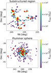 |
Fig. 1 Position of the low- and high-mass stars in the synthetic stellar clusters: Substructured region in the top panel, and Plummer sphere in the bottom panel. |
4.4 Testing the three methods for evaluating the FUV flux on synthetic stellar clusters
The three approaches for evaluating the FUV flux described in the previous section, in particular, the effectiveness of using the local density function to infer the 3D separation between stars in the same star-forming region, were examined through synthetic stellar clusters. In order to highlight the dependence of the density profile on the geometry of the star-forming region, we simulated two regions with identical numbers of high-mass (20) and low-mass (340) stars, but with differing geometries: The first region presented internal substructures, and the second region was modelled as a Plummer sphere (to resemble a spherically symmetric cluster). They are shown in the top and bottom panels of Fig. 1. The substructured synthetic cluster was based on a random subset from the spatial distribution of stars in Winter et al. (2024), considering the simulation snapshot at 1 Myr. Assuming isotropy, the density profile associated with the substructured region depends on the separation between pairs of stars. Conversely, under the condition of spherical symmetry around the centre of the region, as in the case of the Plummer sphere, the density profile is a function of the distance from the centre. The surface and volume density profile of the two simulated regions are shown in Fig. 2. For the substructured region,  , which consists of the Abel transform of
  , can be analytically prescribed by a double power law that is truncated exponentially,
![$\hat \rho (r) = \left\{ {\matrix{ {{\alpha _1}{r^{ - {\beta _1}}},} \hfill & {r \le {r_{\lim }},} \hfill \cr {{\alpha _2}{r^{ - {\beta _2}}}\exp \left[ { - {{\left( {r/{r_{\rm{b}}}} \right)}^{ - \gamma }}} \right],} \hfill & {r > {r_{{\rm{lim}}}},} \hfill \cr } } \right.$](/articles/aa/full_html/2025/03/aa53011-24/aa53011-24-eq20.png) (7)
(7)
where r is the separation between pairs of stars in 3D space (spherical coordinate), normalized to 1 pc in our expressions, and the parameters adopted in the presented case are α1 = 2 × 10⁻⁶, β1 = 2.8, α2 = 5 × 10⁻⁵, β2 = 1.3, the length-scale of the cluster rb = 25 pc (which sets the boundary of the cluster), γ = 2.6, and the limit separation rlim = 0.1 pc, which sets the change of the power-law steepness. These parameters vary based on the specific geometry of the region. The Plummer volume density profile was
 (8)
(8)
where r is the distance from the centre of the cluster in 3D space, and we assumed a Plummer radius of 1 pc and α ≃ 2.4. The density profiles adopted for the various star-forming regions we investigated are summarised in Appendix A.
We evaluated the FUV flux experienced by the low-mass stars due to the irradiation of the high-mass stars using the three approaches described in Sects. 4.1, 4.2, and 4.3. In particular, in order to apply the distance sampling method, we introduced an error on the distance of the stars comparable to the length scale of the region (∼25 pc for the substructured region, and ∼1 pc for the Plummer sphere), which is relatively large compared to the median parallax error in the most nearby regions (e.g. Taurus and Lupus), but is reasonable in more distant regions (e.g. Orion). In Fig. 3 the FUV fluxes resulting from using the three approaches are compared with the true values. Method 1 (Sect. 4.1), shown in yellow in Fig. 3, tends to significantly underestimate the actual flux by some orders of magnitude for some stars. This result highlights the error in the FUV flux that can result from sampling Gaia parallaxes and parallax uncertainties, and the power of our proposed approach. The use of Method 2 (Sect. 4.2) leads to a general overestimate of the flux. Specifically, the fraction of total FUV fluxes reproduced (within 1σ) by Method 1 is 1.3% for the substructured cluster and 21% for the Plummer sphere, while Method 2 reproduces the ∼7.5% of the true values in both cases. The local density function (Method 3) yields FUV fluxes that are consistent with the true values within 1σ error bars for 48% of the low-mass stars in the substructured region and 68% of the low-mass stars in the Plummer sphere case. For the substructured region, we obtained a smaller fraction of successfully reproduced fluxes with respect to the Plummer sphere. This is caused by the fact that we neglected the correlation between stellar pairs when employing the Bayes theorem. Specifically, in our approach, the 3D separation of each pair of low-mass – high-mass star is independently sampled from a cumulative distribution function (CDF). However, the separation between each pair of stars is not completely independent from the others, and a covariance term should be included in the analytic formulation. When this term is not accounted for, the flux uncertainty is underestimated in general. However, the uncertainty in the flux is more strongly underestimated as the number of massive stars that contribute to the flux rises. Therefore, if a star-forming region hosts a small number of massive stars, the error caused by neglecting the covariance term is relatively small. A more detailed analytic work is required to account for this term, together with further testing on simulated clusters. As the resulting fluxes reproduce within the error bars a substancially larger fraction of true values, this study is left to future investigation. Conversely, in the Plummer sphere, as all the separations are defined with respect to the fixed centre of the cluster, we did not investigate each stellar pair independently, but the entire cluster: We sampled from a CDF the 3D separation of all the stars from the centre, generating entire random clusters, and then we evaluated the FUV flux within each cluster.
The fact that Method 3 (Sect. 4.3) yields more than twice the percentage of FUV fluxes consistent with true values compared to other methods highlights the strength and advantage of the approach we propse over the investigated alternative methods.
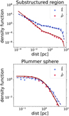 |
Fig. 2 Surface density |


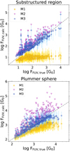 |
Fig. 3 Comparison between the true FUV flux experienced by the low-mass stars as evaluated from the simulated clusters, and the value resulting from applying the three approaches described in Sects. 4.1 (M1), 4.2 (M2), and 4.3 (M3). |
5 Results: A catalogue of FUV flux values for nearby discs
In this section, we present the FUV flux estimate resulting from employing the three approaches introduced in the previous section, at the position of the disc-hosting stars in the selected star-forming regions. We refer to Sects. 5.1 and 5.2 for the investigation of the most nearby regions and regions in Orion and Serpens, respectively. The extended list of FUV fluxes and uncertainties for the considered discs in the various star-forming regions is available in Table B.1. In Sect. 5.3 we investigate the correlation between the FUV flux and the disc dust mass.
5.1 Regions within 200 pc of the Sun
The nearest star-forming regions included in this work contain only a few late B-type and early A-type stars. Therefore, we expect the FUV irradiation to be lower than in more distant and massive regions. Moreover, due to their proximity to Earth, the line-of-sight distance of these stellar objects is known with greater precision, which should result in negligible differences when applying the three different methods for the flux calculation. However, if one or more of the few massive stars are in the close proximity of discs, the resulting FUV irradiation may not be negligible and could significantly influence the disc evolution.
In Fig. 4, we show the FUV flux resulting from applying the three approaches described in Sect. 4 to the discs in the most nearby regions. The three methods proposed for the calculation of the FUV flux provide a conservative estimate (Method 1), an overestimate (Method 2), and our best estimate (Method 3). In order to apply Method 3 (Sect. 4.3), we derived the local density distribution function associated with each region by using the membership catalogues from Luhman (2022b) for Upper Sco and Lupus, Luhman (2020) for Lupus, Luhman (2023) for Taurus, Galli et al. (2021) for Cham I and Cham II, Grasser et al. (2021) for ρ Oph, and Esplin & Luhman (2022) for CrA. The analytic expression that better describes the local density profile of these regions is a double power law truncated close to the length scale of the star-forming region (approximately the width of the region on the sky plane). The parameters of the expression for each region are listed and discussed in Appendix A.
The difference between the three methods is evident in Upper Sco, ρ Oph, Cham I, and CrA. Upper Sco presents the highest number of B-type stars of the considered regions, ∼50 (Luhman 2022b), and where external irradiation was demonstrated to substantially contribute to shaping disc properties (Anania et al. 2025). The massive and hot stars in this region are mostly B8V and B9V, and the only O9 is ζ Oph, which is located at a large separation from the considered discs and therefore does not influence the total flux significantly. The median FUV flux in Upper Sco provided by our best estimate is ∼20 G0 . A similar median is found in ρ Oph, which is located close to the Upper Sco region and contains younger protoplanetary discs with large parallax uncertainties (or no parallax measurements) due to the presence of dense material part of the natal molecular cloud. In this region, ∼90% of the total irradiation at the position of the disc-hosting stars is produced by the multiple system of massive stars ρ Oph itself (B2IV+B2V, Abt 2011). At lower irradiation levels, the presence of massive stars in the close proximity of discs is relevant in Cham I and CrA, where the disc irradiation presents a clear dependence on the separation from the closest massive stars, which are HD 97300 (B9V, Houk & Cowley 1975) and HD 96675 (B5V, Siebenmorgen et al. 2020) in ChamI, and HD 176386 (B9V, Murphy et al. 2020) in Cra. These stars cause the high flux registered for a large sample of discs, with respect to the median, as shown in Fig. 4. In these cases, it is evident that the distance uncertainty sampling approach tends to underestimate the flux, especially when discs are close to massive stars. This occurs even in clusters with only a few massive stars and where the line-of-sight distances are known with higher precision than in more distant regions. The disc-hosting star with the highest FUV flux in CrA is 2MASS J19013912-3653292 (HD 176386B), which forms a binary system with the B9 star HD 176386. The close proximity to this massive star results in the high observed flux.
Conversely, in Cham II, no significant B-type stars are found near the considered discs, and therefore, the overall flux is determined by field stars, non-members of the region, and the best estimate coincides with the result provided by the sole distance uncertainty sampling approach. Taurus and Lupus show similar results, with few discs being very close to B9 stars. The complete list of FUV fluxes with associated uncertainties for individual discs can be found in Table B.1.
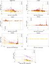 |
Fig. 4 FUV flux experienced by discs in seven regions located ≲200 pc from the Sun. The three approaches we used to evaluate the FUV flux are presented in yellow (Method 1), purple (Method 2), and orange (Method 3). The dashed lines show the median FUV flux value for each calculation method and region. x-axis: Distance from the most massive star, or the centre of the region (when the distribution of OBA stars, and therefore FUV fluxes, is approximately uniform in the region). |
5.2 Orion and Serpens
In Figs. 5 and 6, we present the FUV flux evaluated at the position of the disc-hosting stars in the selected star-forming regions in Orion and Serpens. The flux estimate provided by using our novel approach ( Method 3, Sect. 4.3), shown in orange in Figs. 5 and 6, was evaluated considering the local density distribution function derived by using known stellar membership of each star-forming region from various catalogues retrieved from the literature. Specifically, we used Kounkel et al. (2018) for the ONC, σ Ori, λ Ori, and 25 Ori, Da Rio et al. (2012) and Fang et al. (2021) for the ONC, Žerjal et al. (2024) for σ Ori and NGC 2024, Suárez et al. (2019) for 25 Ori, and the updated sample of members of NGC 1977 by Kim et al. (in prep.). In regions presenting a 2D nearly centrally concentrated geometry, which in our sample correspond to the ONC, σ Ori, λ Ori, and 25 Ori regions, the local density profile was defined as the function of the separation from the centre of the region, as discussed in Sect. 4.4. The analytic expression that better describes this profile is an exponentially truncated single power law, which was already known in previous works for the ONC (e.g. Da Rio et al. 2012). In the case of NGC 2024, the confirmed stellar census contains too few stars that complement the disc-hosting stars included in our study, spread across various separations, which makes it difficult to recover enough stars per unit separation to derive a reliable density profile. Therefore, our statistical approach cannot be fully trusted, and we only present the FUV fluxes obtained through Method 1 (Sect. 4.1), and Method 2 (Sect. 4.2). Additional details on the derivation and reliability of the density profile, along with the specific parameters used in the calculation, are discussed in Appendix A.
For the Serpens region, we used the Gaia DR2 membership census by Herczeg et al. (2020) and the young stellar objects (YSOs) catalogue of Anderson et al. (2022) to derive the local density profile of the three main extended sub-regions, which are NE, Main, and South. In Fig. 6, the investigated ClassII discs in the southernmost region of Serpens South, referred to as Far South, are shown separately from the others. This distinction highlights the dependence of the flux on the separation from the most massive stars, which are IRS1a (O9.5V) and 2MASS J18273952-0349520 (B1.5V, Drew et al. 1997), located in Serpens South (near the HII region Westerhout 40, Shenoy et al. 2013), and Far South, respectively. The highest level of irradiation is found near the HII region Westerhout 40 (W40), where a small group of massive stars is concentrated (Anderson et al. 2022). We refer to Appendix A for the 2D sky maps of the selected disc sample and neighbouring massive stars included in this work, corresponding to each star-forming region.
The average FUV flux is significantly higher in the considered Orion and Serpens regions (with the exception of Serp NE and Serp Main) compared to the closest regions (Fig. 6). The flux estimate provided by involving Method 3 reaches ∼105– 106 G0 in the ONC, where the total flux is dominated by the most luminous O-type and early B-type stars, while field stars only contribute ∼1% of the total flux on average. Method 1 (Sect. 4.1) results in a nearly flat distribution of the FUV fluxes in all the regions, with a median value ≲10 G0 (as shown in yellow in Figs. 4, 5, and 6).
Method 2 and Method 3 both demonstrate a clear dependence of the flux on the distance from the most massive and luminous star in the region, as shown on the x-axis of the panels in Fig. 5.
As for the synthetic cluster, we show that Method 1 using real parallax errors from Gaia DR3 and Hipparcos severely underestimates the FUV flux, while placing constraints based on the 2D geometry of a star-forming region can result in a more accurate FUV estimate.
5.3 Correlation with disc properties: Dust disc mass
Externally irradiated discs can be significantly depleted in their gas and dust components (e.g. Owen et al. 2012; Sellek et al. Sellek et al.). In order to understand the impact of external photoevaporation on the disc evolution and composition, it is crucial to investigate the relation between disc properties and the external radiation they experience. In this section, we focus on the dust disc mass because the gas disc mass and disc size are more challenging to determine and are only available for a few discs in regions at distances larger than ∼200 pc.
The dust content in discs is a more accessible quantity and can be associated with the thermal emission at (sub-)millimeter wavelengths, assuming optically thin emission and setting a certain dust temperature and opacity (e.g. Miotello et al. 2023). The dust disc mass as retrieved from continuum observations is available for part of the investigated disc sample in 12 of the 14 regions (the discs of 25 Ori and NGC 1977 currently lack dust mass measurements). We selected from each of these 12 regions the discs with a measured dust mass. In Fig. 7, we show the median FUV flux as a function of the average age of the region, colour-coded based on the median dust disc mass. The uncertainties on the FUV flux are the 16th and 84th percentiles of the distributions. The median FUV flux of NGC 2024 was obtained by using 2D projected separations from the OBA stars members of the region because the local density profile of the region, which is needed to apply the method proposed in this study, cannot be reliably derived here. However, since the NGC 2024 disc sample presents dust mass measurements, we decided to show the results, taking into account that the median flux value is an overestimate of the actual flux.
Figure 7 shows that less massive discs are generally observed in older regions, a trend that has been extensively investigated by disc surveys in the most nearby star-forming regions (e.g. Manara et al. 2023). However, protoplanetary discs in more and less irradiated regions are expected to evolve differently, and therefore, the disc properties in different regions cannot be compared on the basis of the age alone, but the irradiation from the environment should also be considered. Theoretical and numerical models predict that discs exposed to stronger external irradiation deplete more quickly (e.g. Winter & Haworth 2022), and therefore, we would expect to observe less massive discs in more highly irradiated environments. Observations within individual star-forming regions, such as σ Ori and the ONC, support this prediction, showing a clear dependence of disc millimeter flux emission on FUV flux, where the FUV flux values involved were obtained considering 2D projected separations from the closest massive stars (Ansdell et al. 2017; Maucó et al. 2023; Eisner et al. 2018). This raises the question of whether a similar correlation might hold on a larger scale in multiple starforming regions based on a more accurate estimate of the FUV fluxes. Firstly, we investigated this potential correlation from a region-averaged perspective, considering a median dust disc mass and the FUV fluxes (evaluated using Method 3, Sect. 4.3) in each region, as presented in Fig. 7. Subsequently, we focused on the distribution of dust disc masses and FUV fluxes in regions with a similar age, as shown in Fig. 8.
No clear correlation between the median dust mass and the median FUV flux was identified (Fig. 7). However, several considerations need to be addressed. First of all, the regions in Orion and Serpens presenting high median FUV fluxes in Fig. 7 are very young. This might explain the high dust mass observed with respect to what is measured in the most nearby regions, as external photoevaporation did not have enough time to significantly remove disc material. Moreover, interstellar dust can efficiently shield discs from high-energy external UV photons during the first half million years of the disc (Ali & Harries 2019), and therefore, the detected discs might have experienced intense UV radiation only very recently. However, in more distant regions, the observations are biased toward detecting more massive discs, leading to median dust disc masses that are not entirely representative of the regions. Additionally, the stellar mass distribution is not homogenous in Serpens, Orion, and the nearest regions. More distant regions present only a few objects that were identified as low-mass stars (≲0.3 M⊙) and many more are lacking stellar mass measurements.
Figure 7 shows a clear lack of information on the dust disc mass at intermediate- to high-irradiation levels (>102 G0) with respect to less irradiated regions.
We considered region-averaged values so far, and we now focus on individual values by dividing the disc sample into age bins. We considered regions with a similar average age as the discs disperse over time. Specifically, we considered the age range ~1–3 Myr, where more than two regions present available dust masses. The selected regions are Lupus, Taurus, Cham I, Cham II, CrA, σ Ori, and the ONC. Due to the high concentration of dust mass measurements at low FUV fluxes compared to intermediate- and high-irradiation levels, we divided our dust disc mass sample into flux bins of varying width. We show the distribution of the median dust masses (in each bin) against the distribution of fluxes in the histograms in Fig. 8. The bin widths were chosen based on the number of objects and upper-limit dust masses in each region. Specifically, the sample of the most nearby discs, covering ~1–100 G0, was divided into three parts, as was the σ Ori sample, which covered fluxes from ~102 to ~2 × 10⁴ G0. The ONC disc sample, which consists of detections and non-detections in Eisner et al. (2018), was divided into ~40 stars each, with at least four detections in each bin. Since in the ONC ~60% of the total disc sample is undetected, the median dust disc mass is dominated by upper-limit dust masses (shown as dashed black lines in the top panel of Fig. 8) and is comparable to the observed median in the other regions. Due to the known dependence of the dust mass on the stellar mass (e.g. Manara et al. 2023), the medians can be highly influenced by the range of stellar masses covered. In order to reduce the effect produced by the dependence on stellar mass, we restricted the disc sample in these regions to the relatively high-mass stars (M⋆ > 0.4 M⊙ ), which are the majority detected in σ Ori. The results are shown in the central panel of Fig. 8. We did not include the ONC in this panel because the stellar mass is defined for only one-third of the total disc sample. A decrease in dust disc mass is visible between ~103 and ~104 G0, and it is related to σ Ori (Fig. 8 central panel), where this trend was found previously (Ansdell et al. 2017; Maucó et al. 2023). This is now supported by the use of our updated FUV flux estimate. The correlation in σ Ori is more pronounced when it is restricted to high stellar masses (Fig. 8). A weaker negative dependence of the dust mass on the external flux appears in the ONC, which is more clearly visible in the 84th percentile of the mass distribution, as the median is highly influenced by the undetected objects. The lack of stellar properties and disc millimeter continuum detections at intermediate- to high-irradiation levels limits our ability to draw more exhaustive conclusions for a wide range of distances, regions, and FUV fluxes. Therefore, we strongly support explorations of this parameter space in future observations. In Fig. D.1, we show that we found a tentative correlation between individual dust disc masses and FUV fluxes for objects in the age range of 1–3 Myr. However, the lack of information on stellar mass and dust disc mass above 102 G0 prevents us from strongly supporting the derived correlation.
When we applied the same study to the oldest regions of our sample, which are Upper Sco and λ Ori, we only detected a small decrease in the median dust mass from lower to higher FUV fluxes (from Upper Sco to λ Ori). The results are shown in the bottom panel of Fig. 8. As the disc sample is limited to only two regions, the data are insufficient for a deeper statistical investigation to determine whether the small decrease in the dust disc mass is due to external FUV irradiation or observational biases. Future dust mass measurements of 25 Ori discs will offer crucial data to further explore the relation.
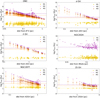 |
Fig. 5 FUV fluxes experienced by discs in six star-forming regions in Orion. The different colours correspond to the different methods for the calculation of the FUV flux, as introduced in Sect. 4. The dashed lines show median FUV flux values for each region and for the calculation method. The x-axis contains the distance from the most massive star in the region. In NGC 2024, the local density distribution method cannot be applied (and therefore, no orange points lie in that panel), as an accurate density profile of the region cannot be currently retrieved. |
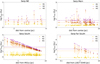 |
Fig. 6 FUV flux experienced by discs in the Serpens region. Based on the sub-region in Serpens where they are located, the discs were divided into NE, Main, South, and the most southern part, Far South. Our flux estimates using Method 1, Method 2, and Method 3 (Sect. 4) are shown in yellow, purple, and orange, respectively. The lines show the median fluxes resulting from the three approaches. x-axis: Distance from the most massive star, or the centre of the region (if no strong dependence on the most massive star was found). |
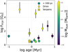 |
Fig. 7 Median FUV flux as a function of the estimated age of the regions. Each dot represents a star-forming region in this work and is colour-coded based on the median dust disc mass available for the sample of discs. NGC 1977 and 25 Ori are not included because they lack dust disc mass measurements. The FUV flux presented for NGC 2024 is evaluated using Method 2 (Sect. 4.2). |
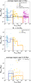 |
Fig. 8 Dust disc masses and FUV fluxes for the regions with average age 1–3 Myr (top and central panel) and 5–10 Myr (bottom panel). The histograms show median dust disc masses in flux bins, including upper limits (shown as coloured triangles). The dotted histograms contain the 84% of the distributions. The top panel presents the median upper limit dust mass in each region as dashed black lines. The central panel only includes objects with a stellar mass >0.4 M⊙, and no upper limit in dust disc mass is present in σ Ori. The ONC is not included in this plot as the stellar mass is only defined for about one-third of the total disc sample. |
6 Discussion
We used the available information on the 2D geometry of a starforming region to compute the best estimate of the FUV flux at the position of a sample of disc-hosting stars (Method 3, Sect. 4.3). In this section, we discuss the FUV fluxes obtained for each region (Sect. 6.1), the uncertainties, limitations, and future improvements of our proposed method (Sect. 6.2), and the correlation with the disc properties (Sect. 6.3).
6.1 FUV flux in the star-forming regions
Figure 9 presents the cumulative distributions of the resulting FUV fluxes in the various regions, divided into the most nearby regions (left panel), regions in Orion (central panel), and regions in Serpens (right panel), for better visualisation. In Fig. 10 we provide for each region the distribution of the median FUV fluxes at the position of disc-hosting stars. Discs in Orion experience the highest levels of irradiation of the studied regions, particularly those in the ONC and NGC 20245. However, we verified that even in regions in which the median irradiation is one hundred times lower than in the ONC, the flux distributions still reach moderate and high levels (102–103 G0). This is due to late B-type and early A-type stars, which are closely located to disc-hosting stars, and it underlines the importance of considering the external irradiation even in moderately irradiated regions. The median incidental external FUV flux on disc-hosting stars in the lowest irradiated regions, which are ChamII, Taurus, Serp NE, and Serp Main, is ∼2–3 G0 , which is induced by field massive stars that are not members of the star-forming regions themselves. Upper Sco and ρ Oph present in median the highest FUV irradiation field in the most nearby regions because of the numerous massive stars in the Sco-Cen OB association (Wright et al. 2023). The disc truncation due to external photoevaporation can efficiently reduce the disc mass and size (with consequences for the planet formation and composition), even below 100 G0 , as demonstrated by numerical models and by a comparison with observations (Anania et al. 2025). Therefore, it is essential to be aware of the irradiation level in the most nearby regions for interpreting the observations. The median FUV fluxes on disc-hosting stars in star-forming regions in Orion range from ~20 G0, which is registered in 25 Ori, to ~5 × 10⁵ G0 in the ONC. The FUV flux in Serpens is dominated by the irradiation produced by the O-type star and the early B-type stars close to Serp South and the HII region W40.
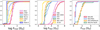 |
Fig. 9 Cumulative distributions of the median FUV fluxes experienced by discs in the regions selected in ≲200 pc (left panel), Orion (central panel), and Serpens region (right panel). The flux values are the best estimate evaluated using Method 3 (Sect. 4.3). The exception is NGC 2024, where we evaluated the FUV fluxes using Method 2 (Sect. 4.2). We consider them as overestimates of the actual fluxes. |
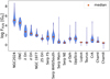 |
Fig. 10 Distributions of the FUV fluxes for the star-forming regions. The median of the distributions is shown in orange. NGC 2024 fluxes are overestimates of the actual values because we used Method 2 (Sect. 4.2) to compute the FUV flux as we lacked information to accurately derive the local density profile. |
6.2 Uncertainties, limitations of the model, and future improvement
The primary sources of uncertainty in the flux calculation are the relative (3D) distances between massive stars and disc-hosting stars and the FUV luminosity of massive stars. We neglected the latter in most cases, and we now justified this and show that this causes a small effect.
In the flux calculation, the uncertainty in FUV luminosity is caused by the uncertainty in the effective temperature of massive stars. Because the effective temperature of most of the OBA stars is defined in the Astrophysical Parameters (ESPHS) pipeline provided by Gaia DR3, we have access to the temperature uncertainty, and we used it to investigate the implications on the final FUV flux value. In the ESPHS pipeline, the error on the effective temperature increases with spectral type. It reaches unreliable temperature values and uncertainties above 25 000 K (Fouesneau et al. 2023). From stellar evolution models, we retrieved that effective temperatures between 8000 and 25 000 K correspond to stellar masses between ~2 and ~ 10 M⊙ (assuming an age of 1 Myr) and to FUV luminosities of ~1034 – 1037 erg s−1. The typical errors on the effective temperatures of massive stars below 23 000 K are a few dozen Kelvin, which translates into errors of a few percent in the FUV luminosity and FUV flux (at a fixed separation). These are negligible errors compared to the uncertainty associated with relative separations. Massive stars in the temperature range [23 000–25 000] K reach temperature uncertainties of a few thousand Kelvin, which result in a FUV flux variation of ~80%. In the last case, where errors cannot be neglected, a more precise temperature estimates is provided by spectral classification tables (Gray & Corbally 2009). Therefore, in order to reduce the impact of the uncertainty in FUV luminosity on the total flux, we retrieved the effective temperature of massive stars above 23 000 K in our calculation (which might present the highly uncertain Gaia ESPHS effective temperature) from a spectral classification, as introduced in Sect. 3.
We proposed the use of the local density profile of a starforming region for the uncertainties in parallax measurements and for determining the 3D separation between pairs of stars in a star-forming region. However, an intrinsic limitation of Method 3 (Sect. 4.3) is the shape of the local density function itself, which is individually derived (and analytically prescribed) for each region. Specifically, the density profile was used in the probability function in Eq. (6), from which we sampled the cumulative distribution function (CDF) to determine the best estimate of the 3D separation between stars. Therefore, an extremely flat density profile results in a nearly uniform probability of 3D separations across a wide range of values (an approximately flat CDF). As a consequence, the uncertainty on the final flux will be large. Conversely, when the initial density profile is extremely steep, the corresponding inverse CDF will be steep as well, presenting its maximum close to the 2D separation value. This leads to a high probability of obtaining fluxes similar to those predicted using the pure 2D separation. Table 2 lists median FUV flux values, with 16th and 84th percentiles of the distribution of the median FUV fluxes and the median relative uncertainty for each region. The relative uncertainties in the various regions generally do not depend on G0. However, in the case of centrally symmetric regions, high FUV flux values can present large error bars because a higher G0 corresponds to a smaller separation between disc and massive stars, which corresponds to the approximately flat part of the spherically symmetric local density function (see the Plummer sphere in Sect. 4.4).
While errors produced by the shape of the local density distribution cannot be removed, future improvements can be made for a better identification of the density profile of star-forming regions. The derivation of accurate local density profiles requires a membership census of star-forming regions that are numerous enough to present a substantial number of stars per unit separation, which permits us to resolve stellar over-densities that influence the shape of the local density function. Therefore, future stellar membership studies in the regions included in this work will improve the precision of the FUV flux calculation method. Moreover, new stellar membership catalogues in additional regions will allow us to apply the method described in this study to a larger stellar sample.
Median FUV flux for the regions.
6.3 FUV flux and disc properties
In Sect. 5.3 we focused on the investigation of the relation between the FUV flux estimate at the position of disc-hosting stars and dust disc masses because the dust disc size, gas disc mass, and size is not measured for the majority of the discs at distances larger than ~200 pc. Of the regions considered in this work, only σ Ori and Upper Sco show a decrease in the dust and gas disc size at higher G0, as presented in Maucó et al. (2023) and Anania et al. (2025). Figure 8 highlights key areas of the FUV flux-age parameter space to explore with future observations in order to investigate in detail how external irradiation contributes to shaping the dust disc content. Specifically, more stellar information (in particular, stellar mass measurements) and deeper disc observations in intermediately and highly irradiated environments (>102 G0 ) in a range of ages of 1–10 Myr would be fundamental to complement our study. Therefore, we strongly encourage measurements of disc properties in other star-forming regions in order to explore the relation with the environmental irradiation.
In proplyds, direct information on the disc mass-loss rate due to external photoevaporation is provided by ionised gas emission lines (e.g. [NII], [Ne III], and [OIII]), which are bright in PDRs and seen at optical wavelengths. One of the most sensitive lines to external UV radiation and a good tracer of the inner region of the wind is [OI] 6300 Å (e.g. Bally et al. 1998; Störzer & Hollenbach 1998), whose luminosity is predicted to increase with the external FUV field strength (e.g. Ballabio et al. 2023). However, at low irradiation levels (≲103 G0), the line luminosity is dominated by the irradiation from the central star, and it cannot be used as tracer of external winds. The observed line luminosity is therefore similar in nearby regions and σ Ori (Mauco et al. 2024). More irradiated regions included in this work, such as the ONC, have too few or missing detections for a statistically reliable study of the optical lines. The physical and chemical characteristics of PDRs are also provided by models and observations of infrared (IR) lines (e.g. rovibrational lines of H2 and CO, mid-IR features of polycyclic aromatic hydrocarbons Hollenbach & Tielens 1999), and are now investigated in detail by JWST in the solar neighbourhood (e.g. Van De Putte et al. 2024). However, the problem of using these lines to trace the external photoevaporation of intermediately and moderately irradiated protoplanetary discs remains, as the radiation from the central star will obscure the contribution of an external UV source. This highlights the need for an independent method to evaluate the FUV radiation in PDR models to accurately compare with observations on the one hand, and alternative PDR tracers in the absence of a proplyd-like morphology on the other.
7 Conclusions
We proposed a novel approach to evaluating the FUV flux, along with its uncertainty, at the position of disc-hosting stars in nearby star-forming regions. We analysed three methods for the uncertainty in the separation between massive stars and low-mass stars in 3D space, which is the main source of the uncertainty in flux calculations. These methods consist of a distance uncertainty sampling (Method 1, Sect. 4.1), a 2D projected separation and distance uncertainty sampling (Method 2, Sect. 4.2), and a local density distribution and distance uncertainty sampling (Method 3, Sect. 4.3). Method 3, our novel approach, involves the use of the local density distribution of a star-forming region under the assumption of isotropy to derive the separation between stars in 3D space, given their 2D separation on the sky plane. The 3D separation was used to compute the FUV flux and its uncertainty. The procedure and main results obtained in this study are summarised below.
We selected a large sample of OBA-type stars and cross-referenced various stellar catalogues to include the contribution of late-type B and early-type A stars to the total FUV radiation, as described in Sect. 3.
Using synthetic clusters, we verified that Method 1 can significantly underestimate FUV flux, while Method 2 leads to upper-limit FUV fluxes (Sect. 4.4). Method 3, which consists of analytically prescribing the local density profile of starforming regions and sampling the derived PDF to obtain 3D separations given 2D separations (Sect. 4.1), yields a significantly larger fraction of FUV fluxes that are consistent within 1σ error bars with true values compared to the other methods.
We provided a catalogue of the FUV flux (and uncertainty) at disc-hosting stars in Taurus, ρ Oph, UppSco, CrA, Lupus, ChamI, ChamII, ONC, σ Ori, λ Ori, NGC 1977, 25 Ori, NGC2024, and the sub-clusters of Serpens. This catalogue is available at the CDS.
In regions without O-type and early-type B stars, the irradiation induced by less massive stars (late-type B and early-type A) can even reach ~102 G0 (Sect. 5). These FUV radiation levels are not negligible for the disc evolution and planet formation, and therefore, the impact of the environment must be taken into account when discs in different regions are compared.
We investigated the relation between the FUV flux and dust disc mass for discs in our sample with dust disc mass measurements in the literature, considering the average age of their star-forming regions (Sect. 5.3). We underline the need for stellar mass and dust disc mass measurements at intermediate- to high-irradiation levels (>102 G0), particularly for regions that are ∼1–3 Myr old (the age range in which most of the disc population is detected), to make reliable claims of a general correlation in different regions.
We included a study of the FUV attenuation caused by interstellar dust extinction (Appendix C). We assumed that the FUV radiation emitted by the massive star members of a certain region is attenuated by an average FUV extinction magnitude retrieved from dust extinction maps, while using an average galactic extinction value for the radiation from field massive stars. The resulting decrease in the median FUV flux per region is not significant (a few G0 , as shown in Table C.1). However, interstellar dust inside individual regions might be not resolved by dust maps and might therefore produce a higher extinction than is assumed.
This study shows that information provided by the 2D geometry of a star-forming region can be used to constrain 3D separations between star pairs within that region. We applied these estimates to compute the FUV flux at the position of nearby disc-hosting stars. This approach can be extended to further regions in future studies.
Data availability
Table B.1 in its extended version is available at the CDS via anonymous ftp to cdsarc.cds.unistra.fr (130.79.128.5) or via https://cdsarc.cds.unistra.fr/viz-bin/cat/J/A+A/695/A74
Acknowledgements
RA and GR acknowledge funding from the Fondazione Cariplo, grant no. 2022-1217, and the European Research Council (ERC) under the European Union’s Horizon Europe Research & Innovation Programme under grant agreement no. 101039651 (DiscEvol). Views and opinions expressed are however those of the author(s) only, and do not necessarily reflect those of the European Union or the European Research Council Executive Agency. Neither the European Union nor the granting authority can be held responsible for them. AJW has received funding from the European Union’s Horizon 2020 research and innovation programme under the Marie Skłodowska-Curie grant agreement No. 101104656.
Appendix A Gallery of investigated star-forming regions and adopted density profiles
The positions on the disc-hosting stars considered in each starforming region included in this work, and the location of their closest massive stars, are shown in Fig. A.1, A.2, and A.2, divided in regions in ≲ 200 pc, Orion regions, and Serpens regions. The OBA stars are colour-coded based on their FUV luminosity, where more massive stars are associated with higher FUV luminosity.
In this work, we employed the Abel’s theorem to derive the volume local density profile of star-forming regions, given an analytical prescription for the surface local density profile (method 3 in Sect. 4.3). As demonstrated in Sect. 4.4, the local density profile can be analytically described by a double power law with exponential cut off for substructured regions, or by a truncated single power law (or a Plummer profile) for centrally concentrated regions. The parameters for the power law profiles, as applied to the star-forming regions in this study, are listed in Table A.1. The terms reported in the Table refers to the expressions:
![$\hat \rho (r) = \left\{ {\matrix{ {{\alpha _1}{r^{ - {\beta _1}}},} \hfill & {{\rm{ if }}r \le {r_{{\rm{lim}}}},} \hfill \cr {{\alpha _2}{r^{ - {\beta _2}}}\exp \left[ { - {{\left( {r/{r_{\rm{b}}}} \right)}^{ - \gamma }}} \right],} \hfill & {{\rm{ if }}r > {r_{{\rm{lim}}}},} \hfill \cr } } \right.$](/articles/aa/full_html/2025/03/aa53011-24/aa53011-24-eq37.png) (A.1)
(A.1)
where the 3D separation r is normalized to 1 pc, rlim is the limit distance around which the steepness of the power law profile changes, and rb is the boundary radius setting the length scale of the star-forming region. This is valid for a region with internal substructures. For the ONC, σ Ori, λ Ori, and 25 Ori regions, we employed a centrally concentrated geometry, with density profile that is function of the distance from the centre of the region, written as:
![$\hat \rho (r) = {\alpha _2}{r^{ - {\beta _2}}}\exp \left[ { - {{\left( {r/{r_{\rm{b}}}} \right)}^{ - \gamma }}} \right],$](/articles/aa/full_html/2025/03/aa53011-24/aa53011-24-eq38.png) (A.2)
(A.2)
where r is normalized to 1 pc and in Table A.1 the terms α1, β1, and rlim assume null values as they do not enter in this expression.
The accuracy in estimating the volume density profiles requires having a substantial number of stars per unit separation (i.e. a nearly complete stellar census of the star-forming regions), to properly account for the 2D internal geometry. In this study, we retrieved membership catalogues for each region from those available in literature. Assigning the stellar membership requires accurate measurements of positions and proper motions, which becomes increasingly difficult in more distant regions, such as Orion and Serpens in our case. Therefore, the defined density profiles may need refinement as future, updated stellar censuses become available. The confirmed stellar membership of NGC 2024 (Kounkel et al. 2018; Žerjal et al. 2024) consists of stars too spatially separated with respect to the compact sample of discs considered in this work, to reliably make claims about the density profile per unit separation. Thus, our new proposed approach to evaluate the FUV flux cannot be applied in this region, which is not included in Table A.1. However, we provided FUV flux estimates using method 2 (Sect. 4.2), being aware that this is an overestimate of the true value. The density profiles of NGC 1977 and Serpens sub-regions are described by single power law relations (where  is function of the separation between pairs on stars) for distances larger than a defined limit separation, rlim, due to the lack of a complete stellar membership at smaller separations, where the shape of
  is primarily influenced by binary systems. However, we verified that no pairs of disc-hosting star - massive star are present at separations smaller than this limit value, and therefore, the defined profile remains valid for our calculations. The Cham II region does not contain any significant OBA stars, and therefore, we did not use the local density profile to evaluate the FUV flux in this region.
Appendix B Catalogue of the FUV flux on star-bearing discs in nearby regions
The approach presented in this study allows to accurately estimate FUV flux (and its uncertainty). We applied this method to evaluate the FUV flux at the position of star-bearing discs in 14 nearby star-forming regions, compiling a catalogue of the FUV flux for a large sample of stellar objects. The complete table containing the flux best estimates is available at the CDS. Few rows of the table, with specific content of the columns, are shown in Table B.1. For each disc-hosting star, we included the corresponding star-forming region, RA and Dec positions from Gaia DR3, median best estimate FUV flux, and uncertainties as 16th and 84th percentiles of the distribution.
Appendix C The role of the extinction
Interstellar gas and, more importantly, dust can efficiently shield protoplanetary discs from an incoming UV radiation. Quantify the relevance of this process is challenging, as it requires knowledge of the internal geometry of a star-forming region and the column density between discs and massive stars. Moreover, gas outflows produced by massive stars can reduce the attenuating material, contributing to the variation in the irradiation experienced by protoplanetary discs with time (e.g. Bania & Lyon 1980; Jeffreson et al. 2021). Simulations of molecular clouds show that discs in high-mass clouds containing several O-type stars, can be efficiently shielded by FUV radiation during the first ~0.5 Myr of their evolution (Ali & Harries 2019; Qiao et al. 2022). After this shielding time, discs are rapidly subject to higher FUV fluxes. In order to investigate the role of the interstellar dust in attenuating the FUV irradiation, we used the 3D dust extinction map provided by Lallement et al. (2022), which uses Gaia and 2MASS photometric data to covers a volume of ~ 6 kpc × 6 kpc × 800 pc around the Sun, reaching resolution of few pc. As the resolution limit of this map is too large to resolve cloud substructures and accurately quantify the column density of material between disc-hosting stars and massive stars in a same star-forming region, where the separation between them is smaller than ~5 pc, we retrieve from the 3D dust map an average extinction magnitude value for each region. This value is included in the calculation of the FUV flux produced by the massive stars internal to a certain region to the disc-hosting stars of the same region. We converted visual magnitudes, provided by the dust map, in FUV magnitudes using a factor AFUV /AV 2.7 (Cardelli et al. 1989; Salim & Narayanan 2020). For the field massive stars (those outside the considered region) we assumed an average galactic extinction value of ~3AV ≃ 2.1 mag kpc−1, as in the work of Cleeves et al. (2016). The individual FUV flux corrected for the UV extinction magnitude is:
 (C.1)
(C.1)
where FFUV, comp is our flux best estimate and AFUV is the average extinction magnitude in the FUV range of wavelengths. In Table C.1 we show the average extinction magnitude for each region, derived from the 3D dust extinction map and converted to FUV wavelengths, the median FUV flux computed using the local density distribution (Method 3, Sect. 4.3), which provides our best estimate of the flux, and the flux value corrected by the UV extinction. We distinguish between the percentage of flux reduction caused by massive hot stars internal the star-forming region (members) and external (field stars). In general, the median FUV flux per region is not drastically reduced by extinction. Since massive stars internal to a region are located closer to discs than field massive stars, their irradiation is less attenuated. In regions like the ONC, where the FUV flux is dominated by few massive stars very close to discs, the extinction correction to the total FUV flux is minimal. In these cases, even though the FUV flux reduction from field stars can be significant (∼25 % for the ONC, ∼40 % for λ Ori), the total FUV flux decrease is negligible (≲1%).
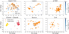 |
Fig. A.1 2D sky maps showing the positions (RA, Dec) of discs and neighbouring massive stars in the nearby star-forming regions included in this work. ChamI and ChamII are shown together due to their small relative distance. |
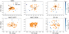 |
Fig. A.2 2D sky maps showing the RA and Dec position of the disc sample and neighbouring massive stars in the Orion regions. |
We provided a tentative estimate of the impact of the dust extinction in attenuating FUV photons incident on disc-hosting stars assuming, for the disc-hosting stars of a certain region, that the FUV radiation emitted by massive stars members of that region is attenuated by the average UV extinction magnitude provided by dust extinction maps at that location, and applying an average galactic extinction to the FUV radiation emitted by massive stars outside the region. The results presented in Table C.1 show that the median FUV flux per region is not significantly reduced by extinction. However, we highlight that the extinction magnitudes used are average values based on a dust map with low resolution for our scopes, meaning that intra-star extinction due to dust material within a single region might be higher than what assumed. Future improvement will be possible with the availability of 3D high-resolution dust extinction maps of star-forming regions.
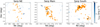 |
Fig. A.3 2D sky maps presenting the location (RA, Dec) of discs and neighbouring massive stars in the Serpens sub-regions. |
Parameters of the volume density profiles used for the star-forming regions included in this work.
FUV flux at the position of the considered discs in 14 nearby star-forming regions.
Appendix D Tentative relation between dust disc mass and FUV flux across regions
A clear dependence of the disc dust mass (i.e. observed mm flux emission) on the FUV radiation has been observed across individual star-forming regions, such as the ONC (Eisner et al. 2018), σ Ori (Maucó et al. 2023), Serpens (van Terwisga et al. in prep.), and the extended population of Orion targeted by the SODA Survey (van Terwisga & Hacar 2023). For what concerns the SODA disc sample, where a correlation is claimed in van Terwisga & Hacar (2023), we are unable to provide a more FUV flux estimate because, in the extended population of Orion, a confirmed subcluster division (essential to apply the method proposed in this work), is not currently defined. Future sub-cluster division and membership census of Orion will make possible a better FUV flux estimate also for the disc sample in the extended population. We explored the dependence of the dust disc mass from the FUV flux across various regions using the updated FUV flux values and uncertainties. We focus on regions with average age between ∼1 and ∼3 Myr, which is the age range in which statistics is expected to be more robust as more than two regions of our sample present dust disc mass measurements. The result is shown in Fig. D.1. Accounting for upper limits in dust musses and including uncertainties on both mass and FUV flux, we found a negative correlation:
 (D.1)
(D.1)
We highlight that the found correlation, described by Eq. (D.1), is only tentative. Indeed, as discussed in Sect. 5.3, the number of dust mass measurements in the flux range 102 – 104 G0 , for discs in regions with average age 1–3 Myr, is not statistically comparable with the observations in the most nearby regions. Moreover, stellar masses are not measured for the majority of the intermediately and highly irradiated objects included in this study, with a bias toward massive stars among the measurements. Since the dependence of dust disc mass on stellar mass (e.g. Manara et al. 2023) should be considered in this analysis, we refer to future work for a more accurate investigation.
Average interstellar extinction used for each region, and percentage of decrease in FUV flux due to attenuation of radiation from stars members of the region and field stars.
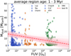 |
Fig. D.1 Tentative correlation between disc dust masses, and FUV flux best estimate in regions with average age 1–3 Myr. Triangles indicate upper limit dust disc masses. Uncertainties in masses and flux, and upper limits, are included in the derivation of the best fit model and not displayed for more clarity in the figure. |
References
- Abel, N. 1826, J. Reine Angew. Math., 1, 153 [Google Scholar]
- Abt, H. A. 2011, AJ, 141, 165 [NASA ADS] [CrossRef] [Google Scholar]
- Ali, A. A., & Harries, T. J. 2019, MNRAS, 487, 4890 [NASA ADS] [CrossRef] [Google Scholar]
- Anania, R., Rosotti, G., Gárate, M., et al. 2025, ApJ, in press [Google Scholar]
- Anderson, A. R., Williams, J. P., van der Marel, N., et al. 2022, ApJ, 938, 55 [NASA ADS] [CrossRef] [Google Scholar]
- Ansdell, M., Williams, J. P., Manara, C. F., et al. 2017, AJ, 153, 240 [Google Scholar]
- Ansdell, M., Haworth, T. J., Williams, J. P., et al. 2020, AJ, 160, 248 [Google Scholar]
- Aru, M. L., Maucó, K., Manara, C. F., et al. 2024, A&A, 687, A93 [NASA ADS] [CrossRef] [EDP Sciences] [Google Scholar]
- Bailer-Jones, C. A. L., Rybizki, J., Fouesneau, M., Demleitner, M., & Andrae, R. 2021, AJ, 161, 147 [Google Scholar]
- Ballabio, G., Haworth, T. J., & Henney, W. J. 2023, MNRAS, 518, 5563 [Google Scholar]
- Bally, J., Sutherland, R. S., Devine, D., & Johnstone, D. 1998, AJ, 116, 293 [NASA ADS] [CrossRef] [Google Scholar]
- Bania, T. M., & Lyon, J. G. 1980, ApJ, 239, 173 [NASA ADS] [CrossRef] [Google Scholar]
- Berné, O., Martin-Drumel, M.-A., Schroetter, I., et al. 2023, Nature, 621, 56 [CrossRef] [Google Scholar]
- Berné, O., Habart, E., Peeters, E., et al. 2024, Science, 383, 988 [Google Scholar]
- Briceño, C., Calvet, N., Hernández, J., et al. 2019, AJ, 157, 85 [CrossRef] [Google Scholar]
- Cardelli, J. A., Clayton, G. C., & Mathis, J. S. 1989, ApJ, 345, 245 [Google Scholar]
- Castelli, F., & Kurucz, R. L. 2004, A&A, 419, 725 [NASA ADS] [CrossRef] [EDP Sciences] [Google Scholar]
- Choi, J., Dotter, A., Conroy, C., et al. 2016, ApJ, 823, 102 [Google Scholar]
- Cleeves, L. I., Öberg, K. I., Wilner, D. J., et al. 2016, ApJ, 832, 110 [Google Scholar]
- Creevey, O. L., Sordo, R., Pailler, F., et al. 2023, A&A, 674, A26 [NASA ADS] [CrossRef] [EDP Sciences] [Google Scholar]
- Cutri, R. M., Wright, E. L., Conrow, T., et al. 2021, VizieR Online Data Catalog: AllWISE Data Release (Cutri+ 2013), VizieR On-line Data Catalog: II/328. Originally published in: IPAC/Caltech (2013) [Google Scholar]
- Da Rio, N., Robberto, M., Hillenbrand, L. A., Henning, T., & Stassun, K. G. 2012, ApJ, 748, 14 [Google Scholar]
- Dotter, A. 2016, ApJS, 222, 8 [Google Scholar]
- Drew, J. E., Busfield, G., Hoare, M. G., et al. 1997, MNRAS, 286, 538 [NASA ADS] [CrossRef] [Google Scholar]
- Eisner, J. A., Arce, H. G., Ballering, N. P., et al. 2018, ApJ, 860, 77 [CrossRef] [Google Scholar]
- Esplin, T. L., & Luhman, K. L. 2022, AJ, 163, 64 [NASA ADS] [CrossRef] [Google Scholar]
- Esplin, T. L., Luhman, K. L., Miller, E. B., & Mamajek, E. E. 2018, AJ, 156, 75 [NASA ADS] [CrossRef] [Google Scholar]
- Facchini, S., Clarke, C. J., & Bisbas, T. G. 2016, MNRAS, 457, 3593 [NASA ADS] [CrossRef] [Google Scholar]
- Fang, M., Kim, J. S., Pascucci, I., & Apai, D. 2021, ApJ, 908, 49 [NASA ADS] [CrossRef] [Google Scholar]
- Fatuzzo, M., & Adams, F. C. 2008, ApJ, 675, 1361 [NASA ADS] [CrossRef] [Google Scholar]
- Fouesneau, M., Frémat, Y., Andrae, R., et al. 2023, A&A, 674, A28 [NASA ADS] [CrossRef] [EDP Sciences] [Google Scholar]
- Gaia Collaboration (Vallenari, A., et al.) 2023, A&A, 674, A1 [NASA ADS] [CrossRef] [EDP Sciences] [Google Scholar]
- Galli, P. A. B., Bouy, H., Olivares, J., et al. 2021, A&A, 646, A46 [NASA ADS] [CrossRef] [EDP Sciences] [Google Scholar]
- Grasser, N., Ratzenböck, S., Alves, J., et al. 2021, A&A, 652, A2 [NASA ADS] [CrossRef] [EDP Sciences] [Google Scholar]
- Gray, R. O., & Corbally, Christopher J. 2009, Stellar Spectral Classification [CrossRef] [Google Scholar]
- Habing, H. J. 1968, Bull. Astron. Inst. Netherlands, 19, 421 [Google Scholar]
- Herczeg, G., Kuhn, M., Zhou, X., et al. 2020, in American Astronomical Society Meeting Abstracts, 235, 156.04 [Google Scholar]
- Hollenbach, D. J., & Tielens, A. G. G. M. 1999, Rev. Mod. Phys., 71, 173 [Google Scholar]
- Houk, N., & Cowley, A. P. 1975, University of Michigan Catalogue of twodimensional spectral types for the HD stars, I. Declinations -90_ to -53_f0. [Google Scholar]
- Jeffreson, S. M. R., Krumholz, M. R., Fujimoto, Y., et al. 2021, MNRAS, 505, 3470 [NASA ADS] [CrossRef] [Google Scholar]
- Kim, J. S., Clarke, C. J., Fang, M., & Facchini, S. 2016, ApJ, 826, L15 [NASA ADS] [CrossRef] [Google Scholar]
- Kounkel, M., Covey, K., Suárez, G., et al. 2018, AJ, 156, 84 [NASA ADS] [CrossRef] [Google Scholar]
- Kunitomo, M., Ida, S., Takeuchi, T., et al. 2021, ApJ, 909, 109 [NASA ADS] [CrossRef] [Google Scholar]
- Lada, C. J., Lombardi, M., & Alves, J. F. 2010, ApJ, 724, 687 [Google Scholar]
- Lallement, R., Vergely, J. L., Babusiaux, C., & Cox, N. L. J. 2022, A&A, 661, A147 [NASA ADS] [CrossRef] [EDP Sciences] [Google Scholar]
- Luhman, K. L. 2020, AJ, 160, 186 [NASA ADS] [CrossRef] [Google Scholar]
- Luhman, K. L. 2022a, AJ, 163, 25 [NASA ADS] [CrossRef] [Google Scholar]
- Luhman, K. L. 2022b, AJ, 163, 24 [NASA ADS] [CrossRef] [Google Scholar]
- Luhman, K. L. 2023, AJ, 165, 37 [NASA ADS] [CrossRef] [Google Scholar]
- Maíz Apellániz, J., Alonso Moragón, A., Ortiz de Zárate Alcarazo, L., & GOSSS Team. 2017, in Highlights on Spanish Astrophysics IX, eds. S. Arribas, A. Alonso-Herrero, F. Figueras, C. Hernández-Monteagudo, A. Sánchez-Lavega, & S. Pérez-Hoyos, 509 [Google Scholar]
- Manara, C. F., Ansdell, M., Rosotti, G. P., et al. 2023, in Astronomical Society of the Pacific Conference Series, 534, Protostars and Planets VII, eds. S. Inutsuka, Y. Aikawa, T. Muto, K. Tomida, & M. Tamura, 539 [NASA ADS] [Google Scholar]
- Maucó, K., Manara, C. F., Ansdell, M., et al. 2023, A&A, 679, A82 [NASA ADS] [CrossRef] [EDP Sciences] [Google Scholar]
- Mauco, K., Manara, C. F., Bayo, A., et al. 2024, in EAS2024, European Astronomical Society Annual Meeting, 1774 [Google Scholar]
- Miller, G. E., & Scalo, J. M. 1978, PASP, 90, 506 [NASA ADS] [CrossRef] [Google Scholar]
- Miotello, A., Kamp, I., Birnstiel, T., Cleeves, L. C., & Kataoka, A. 2023, in Astronomical Society of the Pacific Conference Series, 534, Protostars and Planets VII, eds. S. Inutsuka, Y. Aikawa, T. Muto, K. Tomida, & M. Tamura, 501 [NASA ADS] [Google Scholar]
- Murphy, S. J., Gray, R. O., Corbally, C. J., et al. 2020, MNRAS, 499, 2701 [NASA ADS] [CrossRef] [Google Scholar]
- Ndugu, N., Bitsch, B., & Jurua, E. 2018, MNRAS, 474, 886 [Google Scholar]
- Nguyen, T. K., Viti, S., & Williams, D. A. 2002, A&A, 387, 1083 [NASA ADS] [CrossRef] [EDP Sciences] [Google Scholar]
- O’Dell, C. R., Wen, Z., & Hu, X. 1993, ApJ, 410, 696 [CrossRef] [Google Scholar]
- Otter, J., Ginsburg, A., Ballering, N. P., et al. 2021, ApJ, 923, 221 [NASA ADS] [CrossRef] [Google Scholar]
- Owen, J. E., Clarke, C. J., & Ercolano, B. 2012, MNRAS, 422, 1880 [Google Scholar]
- Pabst, C. H. M., Goicoechea, J. R., Hacar, A., et al. 2022, A&A, 658, A98 [NASA ADS] [CrossRef] [EDP Sciences] [Google Scholar]
- Pecaut, M. J., & Mamajek, E. E. 2013, ApJS, 208, 9 [Google Scholar]
- Perryman, M. A. C., Lindegren, L., Kovalevsky, J., et al. 1997, A&A, 323, L49 [Google Scholar]
- Qiao, L., Haworth, T. J., Sellek, A. D., & Ali, A. A. 2022, MNRAS, 512, 3788 [NASA ADS] [CrossRef] [Google Scholar]
- Qiao, L., Coleman, G. A. L., & Haworth, T. J. 2023, MNRAS, 522, 1939 [NASA ADS] [CrossRef] [Google Scholar]
- Ramírez-Tannus, M. C., Bik, A., Cuijpers, L., et al. 2023, ApJ, 958, L30 [CrossRef] [Google Scholar]
- Ricci, L., Robberto, M., & Soderblom, D. R. 2008, AJ, 136, 2136 [CrossRef] [Google Scholar]
- Salim, S., & Narayanan, D. 2020, ARA&A, 58, 529 [NASA ADS] [CrossRef] [Google Scholar]
- Sellek, A. D., Booth, R. A., & Clarke, C. J. 2020a, MNRAS, 498, 2845 [NASA ADS] [CrossRef] [Google Scholar]
- Sellek, A. D., Booth, R. A., & Clarke, C. J. 2020b, MNRAS, 492, 1279 [NASA ADS] [CrossRef] [Google Scholar]
- Shenoy, S. S., Shuping, R., & Vacca, W. D. 2013, in American Astronomical Society Meeting Abstracts, 221, 349.24 [Google Scholar]
- Siebenmorgen, R., Krełowski, J., Smoker, J., Galazutdinov, G., & Bagnulo, S. 2020, A&A, 641, A35 [NASA ADS] [CrossRef] [EDP Sciences] [Google Scholar]
- Störzer, H., & Hollenbach, D. 1998, ApJ, 502, L71 [CrossRef] [Google Scholar]
- Suárez, G., Downes, J. J., Román-Zúñiga, C., et al. 2019, MNRAS, 486, 1718 [CrossRef] [Google Scholar]
- Van De Putte, D., Meshaka, R., Trahin, B., et al. 2024, A&A, 687, A86 [NASA ADS] [CrossRef] [EDP Sciences] [Google Scholar]
- van Leeuwen, F. 2007, Hipparcos, the New Reduction of the Raw Data, 350 [Google Scholar]
- van Terwisga, S. E., & Hacar, A. 2023, A&A, 673, L2 [CrossRef] [EDP Sciences] [Google Scholar]
- van Terwisga, S. E., van Dishoeck, E. F., Mann, R. K., et al. 2020, A&A, 640, A27 [NASA ADS] [CrossRef] [EDP Sciences] [Google Scholar]
- Vincenty, T. 1975, Surv. Rev., 23, 88 [NASA ADS] [CrossRef] [Google Scholar]
- Vioque, M., Cavieres, M., Pantaleoni González, M., et al. 2023, AJ, 166, 183 [NASA ADS] [CrossRef] [Google Scholar]
- Walsh, C., Millar, T. J., & Nomura, H. 2013, ApJ, 766, L23 [NASA ADS] [CrossRef] [Google Scholar]
- Walsh, C., Herbst, E., Nomura, H., Millar, T. J., & Weaver, S. W. 2014, Faraday Discuss., 168, 389 [NASA ADS] [CrossRef] [Google Scholar]
- Winter, A. J., & Haworth, T. J. 2022, Eur. Phys. J. Plus, 137, 1132 [NASA ADS] [CrossRef] [Google Scholar]
- Winter, A. J., Benisty, M., Shuai, L., et al. 2024, A&A, 691, A43 [NASA ADS] [CrossRef] [EDP Sciences] [Google Scholar]
- Wright, N. J., Kounkel, M., Zari, E., Goodwin, S., & Jeffries, R. D. 2023, in Astronomical Society of the Pacific Conference Series, 534, Protostars and Planets VII, eds. S. Inutsuka, Y. Aikawa, T. Muto, K. Tomida, & M. Tamura, 129 [NASA ADS] [Google Scholar]
- Zari, E., Rix, H. W., Frankel, N., et al. 2021, A&A, 650, A112 [NASA ADS] [CrossRef] [EDP Sciences] [Google Scholar]
- Žerjal, M., Martín, E. L., & Pérez-Garrido, A. 2024, A&A, 686, A161 [NASA ADS] [CrossRef] [EDP Sciences] [Google Scholar]
The FUV flux is given in terms of the Habing unit, G0 (Habing 1968), which quantifies the flux integral over the range of wavelengths [912–2400] A, normalised to the average flux in the solar neighbourhood (1.6 × 10⁻³ erg s−1 cm−2).
We recall that for NGC 2024, we used the flux values derived with Method 2 (Sect. 4.2), because the local density profile cannot be reliably derived in this region. These values are overestimates of the actual FUV flux.
All Tables
Parameters of the volume density profiles used for the star-forming regions included in this work.
FUV flux at the position of the considered discs in 14 nearby star-forming regions.
Average interstellar extinction used for each region, and percentage of decrease in FUV flux due to attenuation of radiation from stars members of the region and field stars.
All Figures
|
Fig. 1 Position of the low- and high-mass stars in the synthetic stellar clusters: Substructured region in the top panel, and Plummer sphere in the bottom panel. |
| In the text | |
|
Fig. 2 Surface density |
| In the text | |
|
Fig. 3 Comparison between the true FUV flux experienced by the low-mass stars as evaluated from the simulated clusters, and the value resulting from applying the three approaches described in Sects. 4.1 (M1), 4.2 (M2), and 4.3 (M3). |
| In the text | |
|
Fig. 4 FUV flux experienced by discs in seven regions located ≲200 pc from the Sun. The three approaches we used to evaluate the FUV flux are presented in yellow (Method 1), purple (Method 2), and orange (Method 3). The dashed lines show the median FUV flux value for each calculation method and region. x-axis: Distance from the most massive star, or the centre of the region (when the distribution of OBA stars, and therefore FUV fluxes, is approximately uniform in the region). |
| In the text | |
|
Fig. 5 FUV fluxes experienced by discs in six star-forming regions in Orion. The different colours correspond to the different methods for the calculation of the FUV flux, as introduced in Sect. 4. The dashed lines show median FUV flux values for each region and for the calculation method. The x-axis contains the distance from the most massive star in the region. In NGC 2024, the local density distribution method cannot be applied (and therefore, no orange points lie in that panel), as an accurate density profile of the region cannot be currently retrieved. |
| In the text | |
|
Fig. 6 FUV flux experienced by discs in the Serpens region. Based on the sub-region in Serpens where they are located, the discs were divided into NE, Main, South, and the most southern part, Far South. Our flux estimates using Method 1, Method 2, and Method 3 (Sect. 4) are shown in yellow, purple, and orange, respectively. The lines show the median fluxes resulting from the three approaches. x-axis: Distance from the most massive star, or the centre of the region (if no strong dependence on the most massive star was found). |
| In the text | |
|
Fig. 7 Median FUV flux as a function of the estimated age of the regions. Each dot represents a star-forming region in this work and is colour-coded based on the median dust disc mass available for the sample of discs. NGC 1977 and 25 Ori are not included because they lack dust disc mass measurements. The FUV flux presented for NGC 2024 is evaluated using Method 2 (Sect. 4.2). |
| In the text | |
|
Fig. 8 Dust disc masses and FUV fluxes for the regions with average age 1–3 Myr (top and central panel) and 5–10 Myr (bottom panel). The histograms show median dust disc masses in flux bins, including upper limits (shown as coloured triangles). The dotted histograms contain the 84% of the distributions. The top panel presents the median upper limit dust mass in each region as dashed black lines. The central panel only includes objects with a stellar mass >0.4 M⊙, and no upper limit in dust disc mass is present in σ Ori. The ONC is not included in this plot as the stellar mass is only defined for about one-third of the total disc sample. |
| In the text | |
|
Fig. 9 Cumulative distributions of the median FUV fluxes experienced by discs in the regions selected in ≲200 pc (left panel), Orion (central panel), and Serpens region (right panel). The flux values are the best estimate evaluated using Method 3 (Sect. 4.3). The exception is NGC 2024, where we evaluated the FUV fluxes using Method 2 (Sect. 4.2). We consider them as overestimates of the actual fluxes. |
| In the text | |
|
Fig. 10 Distributions of the FUV fluxes for the star-forming regions. The median of the distributions is shown in orange. NGC 2024 fluxes are overestimates of the actual values because we used Method 2 (Sect. 4.2) to compute the FUV flux as we lacked information to accurately derive the local density profile. |
| In the text | |
|
Fig. A.1 2D sky maps showing the positions (RA, Dec) of discs and neighbouring massive stars in the nearby star-forming regions included in this work. ChamI and ChamII are shown together due to their small relative distance. |
| In the text | |
|
Fig. A.2 2D sky maps showing the RA and Dec position of the disc sample and neighbouring massive stars in the Orion regions. |
| In the text | |
|
Fig. A.3 2D sky maps presenting the location (RA, Dec) of discs and neighbouring massive stars in the Serpens sub-regions. |
| In the text | |
|
Fig. D.1 Tentative correlation between disc dust masses, and FUV flux best estimate in regions with average age 1–3 Myr. Triangles indicate upper limit dust disc masses. Uncertainties in masses and flux, and upper limits, are included in the derivation of the best fit model and not displayed for more clarity in the figure. |
| In the text | |
Current usage metrics show cumulative count of Article Views (full-text article views including HTML views, PDF and ePub downloads, according to the available data) and Abstracts Views on Vision4Press platform.
Data correspond to usage on the plateform after 2015. The current usage metrics is available 48-96 hours after online publication and is updated daily on week days.
Initial download of the metrics may take a while.