| Issue |
A&A
Volume 695, March 2025
|
|
|---|---|---|
| Article Number | A177 | |
| Number of page(s) | 15 | |
| Section | Extragalactic astronomy | |
| DOI | https://doi.org/10.1051/0004-6361/202452772 | |
| Published online | 18 March 2025 | |
Robust machine learning model of inferring the ex situ stellar fraction of galaxies from photometric data
1
Shanghai Astronomical Observatory, Chinese Academy of Sciences, 80 Nandan Road, Shanghai 200030, China
2
School of Astronomy and Space Sciences, University of Chinese Academy of Sciences, No. 19A Yuquan Road, Beijing 100049, People’s Republic of China
3
Department of Astronomy, Shanghai Jiao Tong University, Shanghai 200240, China
4
Max Planck Institute for Astronomy, Königstuhl 17, 69117 Heidelberg, Germany
5
Instituto de Astrofísica de Canarias, Calle Via Láctea s/n, 38200 La Laguna, Tenerife, Spain
6
Depto. Astrofísica, Universidad de La Laguna, Calle Astrofísico Francisco Sánchez s/n, 38206, La Laguna, Tenerife, Spain
⋆ Corresponding authors; This email address is being protected from spambots. You need JavaScript enabled to view it.
; This email address is being protected from spambots. You need JavaScript enabled to view it.
Received:
28
October
2024
Accepted:
24
January
2025
Abstract
We searched for the parameters defined from photometric images to quantify the ex situ stellar mass fraction of galaxies. We created mock images using galaxies in the cosmological hydrodynamical simulations TNG100, EAGLE, and TNG50 at redshift z = 0. We defined a series of parameters describing their structures, including the absolute magnitude in r and g bands (Mr, Mg), the half-light and 90% light radius (r50, r90), the concentration (C), the luminosity fractions of inner and outer halos (finnerhalo, fouterhalo), and the inner and outer surface brightness gradients (∇ρinner,∇ρouter) and g − r colour gradients (∇(g − r)inner,∇(g − r)outer). In particular, the inner and outer halo of a galaxy are defined by sectors ranging from 45 to 135 degrees from the disk major axis, and with radii ranging from 3.5 to 10 kpc and 10 to 30 kpc, respectively, to avoid the contamination of disk and bulge. The surface brightness and colour gradients are defined by the same sectors along the minor axis and with similar radii ranges. We used the random forest method to create a model that predicts fexsitu from morphological parameters. The model predicts fexsitu well with a scatter smaller than 0.1 compared to the ground truth in all mass ranges. The models trained from TNG100 and EAGLE work similarly well and are cross-validated; they also work well in making predictions for TNG50 galaxies. The analysis using random forest reveals that ∇ρouter, ∇(g − r)outer, fouterhalo, and finnerhalo are the most influential parameters in predicting fexsitu, underscoring their significance in uncovering the merging history of galaxies. We further analysed how the quality of images will affect the results by using SDSS-like and HSC-like mock images for galaxies at different distances. Our results can be used to infer the ex situ stellar mass fractions for a large sample of galaxies from photometric surveys.
Key words: methods: statistical / galaxies: evolution / galaxies: structure
© The Authors 2025
 Open Access article, published by EDP Sciences, under the terms of the Creative Commons Attribution License (https://creativecommons.org/licenses/by/4.0), which permits unrestricted use, distribution, and reproduction in any medium, provided the original work is properly cited.
This article is published in open access under the Subscribe to Open model. This email address is being protected from spambots. You need JavaScript enabled to view it. to support open access publication.
1. Introduction
Galaxies grow by two notable channels, in situ star formation and ex situ galaxy–galaxy mergers, which lead to the formation of different galaxy structures. Galaxy structures (i.e. disks, bulges, and bars identified in the Hubble diagram Hubble 1926) are taken as fossil records of galaxy assembly histories. It is generally believed that disks are formed by in situ star formation from regularly rotating gaseous disks (Fall & Efstathiou 1980); classical bulges are formed by violent processes such as protogalactic collapse or galaxy–galaxy mergers (Toomre 1977); and bars or pseudobulges are the result of secular evolution such as disk instability (Kormendy & Kennicutt 2004). Major mergers are thought to also play a significant role in the formation of stellar halos by destroying stellar disks (Bois et al. 2010, 2011; Pillepich et al. 2015); and minor mergers can cause significant growth of both the stellar and dark matter halos, resulting in a significant increase in the galaxy size (Hilz et al. 2012). Galaxy structures are expected to provide valuable insight into their merger histories.
A great deal of effort has been made in the literature to infer the merger history of galaxies from their morphological structures. However, no promising morphological parameters have been found. Semi-analytical simulations suggest that early-type galaxies can generally be fitted by a double-Sersic profile, and there is a transition radius from in situ dominated regions to ex situ dominated and from the inner steep component to the outer shallower component (Cooper et al. 2013, 2015). There is a similar transition from in situ dominated to ex situ dominated in Illustris simulations (Rodriguez-Gomez et al. 2016). This transition radius or the mass of the outer shallower component has been used as an indicator of the ex situ stellar mass of galaxies (Forbes & Remus 2018; D’Souza et al. 2014; Huang et al. 2013; Spavone et al. 2017, 2020). However, ex situ stars are also found to contribute in the very inner regions of galaxies (Zhu et al. 2022a; Remus & Forbes 2022), and can be dominant at all radii for the most massive galaxies (Tacchella et al. 2019). In particular, with the hydrodynamical cosmological simulation Magneticum, although a large fraction of galaxies still show a transition radius in the surface brightness profile, it does not correspond to the transition from in situ to ex situ dominant, and it is not obviously correlated with the ex situ mass of galaxies (Remus & Forbes 2022).
Although ex situ stars can be distributed throughout the galaxy, the total ex situ stellar mass is still an important parameter as a first-order description of the merger history of a galaxy. Recent works use machine learning tools such as cINN and random forest (Breiman 2001) to study the merger history of galaxies by combing various parameters including stellar mass, stellar populations, and a few morphological parameters: galaxy radius (r90, r50), concentration, luminosity fraction of disk. These models predict ex situ stellar mass fractions well with a typical scatter of ∼0.1 compared to the ground truth with enough input information (Eisert et al. 2023; Shi et al. 2022). Similar model predictions are made using the 2D spatially resolved maps as model input, including the stellar kinematics, stellar age, and metallicity maps, as can be obtained from integral field unit (IFU) observations (Angeloudi et al. 2023, 2024). However, none of the above works finds any morphological parameters more important than the total brightness in predicting the ex situ stellar mass fraction; the radius r90 measured from 3D is found to be important, but considering the observational uncertainty, r90 measured from mock images is still less important (Shi et al. 2022).
The merger history of the Milky Way (MW) and a few nearby galaxies has been quantitatively uncovered through their 3D chemodynamical structures. An ancient massive merger that occurred in the MW about 10 Gyr ago was discovered by the Gaia-Enceledus-sausage structure (Helmi et al. 2018; Belokurov et al. 2018). Multiple merger events have been further quantified by the orbits and chemical properties of stellar populations (Das et al. 2020) and globular clusters (GCs) (Kruijssen et al. 2020) in the MW halo.
However, we cannot resolve the stellar motion and chemical properties of single stars or GCs in most of the nearby galaxies. In the past two decades, integral field unit (IFU) spectroscopic instruments have mapped thousands of galaxies across a wide range of masses and Hubble types (Bacon et al. 2001; Sánchez et al. 2012; Walcher et al. 2014; Emsellem et al. 2011; Croom et al. 2012; Bundy et al. 2015). In principle, information regarding stellar motions and chemical distributions of an external galaxy is included in these IFU data, though all blended along the line of sight (LOS).
Based on the IFU data, two independent methods have been developed to uncover the galaxy merger history. The first tries to constrain the global ex situ fractions (Davison et al. 2021a,b; Boecker et al. 2020) or the mass of satellite mergers (Pinna et al. 2019a,b; Martig et al. 2021) based on the age and metallicity distributions of stars in the inner regions of galaxies obtained from IFU data by full-spectral fitting. This method can identify minor mergers because their accreted stars have a lower metallicity than in situ stars, but they become insensitive to major mergers with overlapping metallicities. The second method is to uncover the internal 3D chemo-dynamical structure of a nearby galaxy by creating population orbit superposition models (Zhu et al. 2020), and to use a dynamically defined hot inner stellar halo as an indicator of merger mass. The hot inner stellar halo, defined by stars on highly radially orbits similar to the MW Gaia-Enceledus-sausage structure, is found to be highly correlated with the total ex situ stellar mass and the most massive merger mass the galaxies have ever experienced (Zhu et al. 2022a). The merger time can be quantified by comparing the stellar age distribution of the disk and other components considering the interaction of the disk and the halo (Zhu et al. 2022b), also in a way comparable to the MW (Belokurov et al. 2018). The merger mass and the merger time for NGC 1380 and NGC 1427 have been determined using this method (Zhu et al. 2022b). Both methods require high-quality IFU data and expensive spectra fitting or dynamical models, thus only being applied to a few case studies.
Inspired by these studies that infer galaxy merger history from the chemo-dynamical structures, we wanted to find morphological structures that mimic the dynamically defined hot inner stellar halo and thus can be applied to a large sample of galaxies from photometric surveys. Using mock images created from the cosmological simulation IllustrisTNG and EAGLE, we investigated whether we can find morphological structures that efficiently trace the galaxy merger history, and we further created models using random forest to predict the ex situ stellar mass of galaxies by only using information obtained from photometric data.
This paper is structured as follows. In Section 2 we describe the mock images and the definition of the morphological parameters extracted from the mock images. In Section 3 we introduce the random forest method. In Section 4 we describe the models that predict fexsitu, and show the influence of the importance of different parameters. In Section 5 we discuss the dependence on the quality of photometric images and on different simulations. We conclude in Section 6.
2. Data
2.1. Cosmological galaxy simulations
Cosmological hydrodynamical simulations for the formation and evolution of galaxies have successfully reproduced galaxies in relatively large cosmic volumes. IllustrisTNG simulations (Pillepich et al. 2018; Marinacci et al. 2018; Nelson et al. 2019a; Naiman et al. 2018; Springel et al. 2018) have been successful in reproducing a wide range of observational findings (Nelson et al. 2019b). These include the galaxy mass-size relation at 0 < z < 2 (Genel et al. 2018), but also the gaseous and stellar disk sizes and heights (Pillepich et al. 2019), galaxy colours, stellar age and metallicity trends at z ∼ 0 as a function of galaxy stellar mass in comparison to SDSS results (Nelson et al. 2018), and resolved star formation in star-forming galaxies (Nelson et al. 2021), as well as the characteristics of the stellar orbit distributions from the CALIFA survey (Xu et al. 2019) and the kinematics of early-type galaxies in comparison to data from ATLAS-3D, MaNGA, and SAMI (Pulsoni et al. 2020). It comprises three flagship runs: TNG300, TNG100, and TNG50 with different cosmological volumes and stellar particle resolutions (see Table 1).
Basic information regarding the publicly available cosmological simulations we use or refer to in this paper.
The EAGLE (Schaye et al. 2015; Crain et al. 2015) simulations have also been shown to successfully reproduce a range of observations of galactic properties, including the galaxy stellar mass function, the Tully–Fisher relation, and the galaxy mass-size relation. The galaxy sizes as a function of stellar mass generally agree with the SDSS results (Schaye et al. 2015). Galactic structures, such as disks and bulges, are well resolved, and the Hubble sequence is in place (Lange et al. 2016; Trayford et al. 2019).
For this work we used the publicly available data of TNG100 and TNG50 (Nelson et al. 2019b) and the fiducial EAGLE simulation (McAlpine et al. 2016). TNG100 and EAGLE were used for most of the analysis; they have similar cosmological volumes and stellar particle resolutions, but are produced by substantially different numerical codes and with different galaxy formation models. The cosmological volumes are large enough that we can have enough galaxies for our analysis, and the spatial resolution is still too high to allow us to investigate the galaxy structures at the sub-kiloparsec scale.
There are 4133 galaxies in TNG100 and 2137 galaxies in EAGLE with M* > 1010.3 M⊙, at z = 0. We eliminated galaxies with ongoing mergers (adopted by eye), which are 673 and 458 in TNG100 and EAGLE, respectively; a few of these galaxies are illustrated in the Appendix (Fig. A.1). There are also some galaxies with an obviously incorrectly defined ex situ fraction caused by the misidentification of its main progenitor galaxy. We identified 102 and 72 such galaxies in TNG100 and EAGLE from their merger tree, and also excluded them from our sample. In the end, we have 3377 and 1620 galaxies from TNG100 and EAGLE, respectively. TNG50 has a higher resolution compared to TNG100, but with a smaller cosmological volume. With a similar selection, we have 443 galaxies from TNG50. The basic information of these three simulations is shown in Fig. 1 and is listed in Table 1.
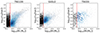 |
Fig. 1. Galaxy stellar mass–size relation of simulations analysed in this paper: (from left to right) TNG100, EAGLE, and TNG50. We chose the stellar mass, M*, defined within a spherical radius of 30 kpc vs. r50 defined from a 2D image. The galaxies kept in our analysis with M* > 1010.3 M⊙ are coloured in blue, the galaxies with ongoing mergers are removed from our analysis and are coloured in grey. |
2.2. Mock images
We created mock photometric images from TNG100 and EAGLE galaxies to mimic the SDSS and HSC observations for nearby galaxies. We took a few steps to create the mock images: First, we read the coordinates and absolute magnitude of the stellar particles for each simulated galaxy and aligned the three main axes with x, y, and z. Second, we smoothed the particles employing the spline kernel that is commonly used to smooth the particles in hydrodynamical simulations (Monaghan & Lattanzio 1985; Monaghan 1992). Third, we projected these galaxies onto the sky plane near edge-on with inclination angles between 80 and 90 degrees. Fourth, we placed the galaxy at a certain distance and divided it into pixels with certain pixel size on the 2D sky plane. Both TNG and EAGLE provide the particle luminosity in a few photometric bands including r and g. We added the luminosity contribution of smoothed particles along the line of sight to construct the light in each pixel. Finally, we convolved the image with a point spread function (PSF) kernel with a certain full width at half maximum (FWHM) using filter2D from OpenCV1 and added sky background noise Σ0.
We did not include more complex effects, such as gas or dust extinction, in our mock images. Our analysis in the following will show that we mainly rely on the parameters related to the stellar halo where gas and dust should not play an important role (Rodriguez-Gomez et al. 2019).
All galaxies are projected nearly edge-on, and we created several versions of mock data by mimicking SDSS or HSC observations; by placing the galaxies at different distances, for each galaxy we created images in the r and g bands. For SDSS-like images, we used a pixel size of 0.396 arcsec, a PSF kernel with FWHM of 1.32 arcsec, and sky background noise Σ0 of 26.86 mag/pixel in the r band, and 27.40 mag/pixel in the g band2, following the typical quality of images in SDSS data release 17 (Abdurro’uf et al. 2022). For HSC-like images, we used a pixel size of 0.168 arcsec, a PSF kernel with FWHM of 0.75 arcsec, and sky background noise Σ0 of 32.5 mag/pixel in the r band and 32.13 mag/pixel in the g band3, which are the typical quality of images in HSC Public Data Release 3 (Aihara et al. 2022).
For SDSS-like observations we created several versions of mock images by placing all galaxies at distances of 40, 100, 200, 400, and 600 Mpc, and for HSC-like observations at 40, 200, 400, 600, 1000, and 1500 Mpc to investigate how the quality of images affect the results. In addition, we created a version of clean images by placing the galaxies at 40 Mpc and not including PSF or background noise for galaxies in TNG100, EAGLE, and TNG50. We note that we only created the clean image for TNG50 galaxies because it is expensive to smooth the particles with large numbers. We use clean images for TNG50 when cross-validating the model with TNG50 in the following analysis.
We show an SDSS-like image in the r band that we created from the TNG100 subhalo ID6 placing it at a distance of 40 Mpc from us in Fig. 2. We use SDSS-like images at 40 Mpc as default for most of the analysis throughout the paper.
 |
Fig. 2. SDSS-like r-band image created from a TNG100 galaxy subhalo 6 at z = 0 projected near edge-on, and placed at the distance of 40 Mpc. Top: 2D image. The sector enclosed by blue is defined as the inner halo (3.5 kpc–10 kpc) and that in red as the outer halo (10 kpc–30 kpc). Bottom: surface brightness profile along the minor axis. The black horizontal line indicates the background noise of the sky Σr, 0; the red and magenta vertical lines mark r50 and r90 obtained from the Petrosian radius. |
2.3. Definition of parameters
Our aim is to uncover the ex situ stellar mass fraction of galaxies (fexsitu). For galaxies from cosmological simulations, we defined the stellar mass of the galaxy M* as the mass of all particles within a 30 kpc sphere of the galaxy. We identified ex situ particles that do not belong to the main progenitor branch but were accreted from other progenitors. Ex situ mass is defined as the mass accreted and that still exists in the galaxy at z = 0. This definition means that we do not consider the mass accreted in the past but stripped by other galaxies in our ex situ mass (Rodriguez-Gomez et al. 2016, 2017, 2019; Pillepich et al. 2018). The ex situ stellar mass fraction (fexsitu) is defined as the ratio of ex situ stellar mass to the total stellar mass of the galaxy at z = 0.
We defined a few parameters that can be directly measured from the mock photometric images and two parameters from the LOS velocity distribution of a single aperture mimicking the single-fibre spectroscopic observation. The parameters we define for each galaxy are as follows:
-
The absolute magnitudes in the r and g bands, Mr and Mg, are determined by the luminosity in the corresponding band of all particles within 30 kpc of the galaxy, which is approximately with the Petrosian aperture as Nelson et al. (2018) shows.
-
Galaxy colour g − r defined as Mg − Mr.
-
Galaxy radii r50 and r90 determined from the r-band mock image. These parameters encompass 50% and 90% of the flux within a mock image. The total flux refers to the Petrosian flux, which is calculated as that within twice the Petrosian radius (Stoughton et al. 2002). The Petrosian radius is defined as the circular radius at which the local surface brightness decreases to 20% of the mean surface brightness within the aperture. In the bottom panel of Figure 2, we mark r50 and r90 of the galaxy defined in this way.
-
Concentration defined as C = 5 × log10(r90/r50) (Conselice 2003).
-
Luminosity fraction of the inner and outer halos, finnerhalo and fouterhalo. The inner and outer halos are defined by a sector with 45 − 135 degrees from the major axis of the disk, with distances ranging from 3.5 to 10 kpc and 10–30 kpc, respectively, as shown in Figure 2. We used r-band luminosity weighted finnerhalo and fouterhalo for most of the analysis, calculated as the ratio of r-band luminosity within the inner and outer halo regions to the total luminosity within 30 kpc. The inner and outer halos are defined to avoid contamination of the disk and the compact bulge component. The separation of the bulge and inner stellar halo at r = 3.5 kpc follows the definition of a dynamically hot inner stellar halo in Zhu et al. (2022a).
-
The inner and outer surface brightness gradients, ∇ρinner and ∇ρouter, along the minor axis by the same sector used for defining halos. The inner gradient ∇ρinner is defined from the centre to 10 kpc, ∇ρinner = (ρ9 − 11 kpc − ρ0 − 3 kpc)/(10 − 1.5), and the outer gradient ∇ρouter from 10 to 30 kpc, ∇ρouter = (ρ29 − 31 kpc − ρ9 − 11 kpc)/(30 − 10), where ρ0 − 3 kpc, ρ9 − 11 kpc, and ρ29 − 31 kpc are taken as the average of surface brightness within the sector and in the radii ranges of 0–3 kpc, 9–11 kpc, and 29–31 kpc, respectively.
-
The inner and outer colour gradients, ∇(g − r)inner, ∇(g − r)outer, along the minor axis, defined in the same regions as ∇ρinner and ∇ρouter, but taking the colour g − r rather than the surface brightness.
-
Velocity dispersion σv and kurtosis h4 from a single aperture spectroscopic observation. We took a single aperture with radius size of 3 arcsec at the galaxy centre, and extracted the LOS velocity distribution from all the particles in this aperture in order to mimic that which could be obtained from a single-fibre spectroscopic observation of each galaxy. We fit the LOS velocity distribution by a Gaussian-Hermit function, and extracted the velocity dispersion σv and the Kurtosis h4 from the Gaussian-Hermit fitting (Gerhard 1993; van der Marel & Franx 1993).
In summary, we defined 12 parameters, Mr, Mg, g − r, r90, r50, C = 5 × log10(r90/r50), finnerhalo, fouterhalo, ∇ρinner, ∇ρouter, ∇(g − r)inner, and ∇(g − r)outer directly measured from the r and g band photometric images. We also defined two parameters, σv and h4, from single-aperture spectra. All the parameters defined are summarised in Table 2. We properly included bias or uncertainties on the 12 parameters directly measured from the images by including observation effects in the mock images. For σv and h4, we did not consider bias or uncertainties caused by real observations.
Observational parameters defined in this paper.
3. Method
3.1. Decision tree
Before introducing random forest, we briefly present the foundational concept of a decision tree. The decision tree (Breiman et al. 1984) is a simple yet highly interpretable machine learning algorithm that aligns with human intuitive thinking, acting as a supervised learning algorithm based on the if-then-else rule. It establishes a mapping between properties and the value of an object in a tree-like structure. In this structure, each node represents an object, each forked path represents a possible property value, and each leaf node corresponds to the value of the object represented by the path from the root node to the leaf node.
3.2. Random forest method
The random forest (Breiman 2001) is an algorithm that uses the ensemble learning concept of bagging to combine multiple decision trees. It can be applied for clustering, classification, and regression analyses. For classifying an input sample, it is subjected to classification by each decision tree, and the classification results of these weak classifiers (i.e. decision trees) are aggregated to form a strong classifier (i.e. random forest). There are two key generation rules for each decision tree within the random forest algorithm. First, with data size N, if we set the training set size to n, then each tree randomly selects a training sample of n (with n < N) from the data set using the bootstrap sample method, resulting in a training set that differs for each tree and contains repeated training samples. Second, of the M features, m features (with m < M) are randomly chosen from M when splitting each node, and the best feature (with the maximum information gain) among these m features is used for node splitting. Throughout forest growth, the value of m remains consistent. The introduction of these two levels of randomness significantly influences the classification performance of the random forest. Their incorporation helps prevent overfitting and enhances noise immunity. During the classification task, each decision tree classifies the newly entered samples, which ultimately contributes to the final output.
For this paper we used the RandomForestRegressor class from the Python package scikit-learn (Pedregosa et al. 2011) to construct the random forest. There are a few important hyperparameters that need to be considered for the random forest configuration: (1) the number of decision trees, nestimators, for which we explore the optimal value in the range of 5–3000; (2) the number of features to consider at each node, nmax-features, given the total features of M, for which we adopted  ; (3) the maximum depth allowed for each tree, nmax-depth, for which we searched for the optimal value within the range of 10–500; (4) the minimum number of samples required for a node to be split nmin-split, for which we seek the best value from the options of [2, 5, 8]; (5) the minimum number of samples required to form a leaf node, nmin-leafrange, for which we explore the optimal value among [1, 2, 4, 8]. We allow a wide range for the two hyperparameters, nestimators and nmax-features, which are considered the most important hyperparameters in the random forest method.
To construct the model, we first divided our data sets into model and validation data sets by fixing the fraction of data in the two sets to be 7 : 3. The model data set was used to train and test the model; therefore, we further separated the model data set into training and testing data sets using the threefold cross-validation method of the GridSearchCV class in the sklearn package (Pedregosa et al. 2011). With the threefold cross-validation method, we randomly separated the model data set into three parts. We took two of the three parts to train the model, and the third to test the model each time, and repeated the processes three times to use the three parts as training and testing, in turn. We finally took the average results of the three models. This method ensures the robustness of the model and reduces the impact of data partitioning on the performance of the model.
We then evaluated the model using the validating data, and the results were quantified using the r-square (r2) metric,
 (1)
(1)
where  is the model prediction, yi is the ground truth, and
  is mean of model predicted value.
We also considered the uncertainty caused by partitioning the model and validation sets by performing the separation at random 50 times. For each separation, we created the model using the model data set and evaluated it using the corresponding validating data set. Finally, we averaged the r2 value from the 50 models.
We understand that the machine learning models created from galaxy simulations may depend on the performance of simulations, including the resolution and physics in the galaxy formation. We created model A using 70% of the galaxies from TNG100 to train the model and the remaining 30% of the galaxies to validate the model. We created model B in a similar way, but using galaxies from EAGLE. For model C, we used EAGLE galaxies to train the model, but TNG100 galaxies to validate the model. For model D, we used TNG100 galaxies to train the model, but EAGLE galaxies to validate the model. The models are summarised in Table 3.
The training and validating data sets used for the four models.
4. Result
4.1. Correlations between observations and fexsitu
We have defined a series of parameters from the mock photometric observations; we used the SDSS-like mock data by placing galaxies at a distance of 40 Mpc for all the analyses in this section. In Figure 3, we show their correlations with the ex situ stellar mass fraction fexsitu for TNG100 and EAGLE galaxies. The tightness of the correlations is quantified by the Spearman rank coefficient of correlation (ρ), with ρ = 1 indicating a perfect positive correlation; ρ = −1 indicating a perfect negative correlation; and ρ = 0 indicating that there is no correlation.
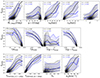 |
Fig. 3. Correlations between the parameters extracted from mock SDSS photometric observations for galaxies at 40 Mpc and the ex situ stellar mass fraction of galaxies. The grey dots are TNG100 galaxies; the black solid and dashed curves are the running median and the ±1σ scatter of the TNG100 galaxies. The blue symbols are for EAGLE galaxies. The Spearman’s rank coefficient(ρ) of each correlation is labelled in the figure. |
The outer surface brightness gradient, ∇ρouter; the outer colour gradient, ∇(g − r)outer; the luminosity fraction of the outer halo, fouterhalo; and the inner halo, finnerhalo, exhibit the strongest correlations with fexsitu compared to other parameters. The magnitude of the galaxy, Mr; the radius of the galaxy r90, r50; the inner surface brightness gradient, ∇ρinner; the concentration, C; and the single aperture velocity dispersion, σ, also exhibit moderate correlations with fexsitu. The galaxy colour, g − r; inner colour gradient, ∇(g − r)inner; and single aperture kurtosis, h4, have a weak correlation with fexsitu.
The correlations between the above observational parameters and fexsitu are similar in TNG100 and EAGLE galaxies. Although the correlations are slightly stronger in the TNG100 galaxies with higher ρ, there are no significant systematic offsets between TNG100 and EAGLE galaxies for the median curves of the correlations shown in Fig. 3. Such correlations also exist and are similar to those in the TNG50 galaxies (see Figure B.1). Thus, these correlations between the observational parameters we defined and fexsitu are independent of the galaxy formation model and the simulation resolution, consistent with the relations found with the dynamically defined hot inner stellar halo (Zhu et al. 2022a).
4.2. The importance of the features
The careful choice of input features plays an important role in achieving the optimal performance of a machine learning model. We evaluated the importance (r2, Equation (1)) of different parameters in predicting fexsitu using random forest. In order to check the dependence on the simulations, we evaluated the importance in four random forest models: models trained and validated by TNG100 and EAGLE galaxies, respectively, and models cross-validated with TNG100 and EAGLE.
We show the importance of the parameters of the four models in Fig. 4. In all four models the outer surface brightness gradient, ∇ρouter; the outer colour gradient, ∇(g − r)outer, the luminosity fraction of the outer halo, fouterhalo; and the inner halo, finnerhalo, are the four with the highest importance for the prediction of fexsitu, consistent with the strong correlations of these parameters with fexsitu shown in Fig. 3.
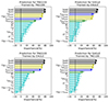 |
Fig. 4. Importance (r2) of the observational parameters in predicting the ex situ stellar mass fraction fexsitu. The top panels are models trained and validated by TNG100 and EAGLE, respectively; the bottom panels are models cross-validated with TNG100 and EAGLE. In each panel the two black points shows the importance of combined parameters: Sub0 including ∇ρouter, ∇(g − r)outer, fouterhalo, finnerhalo, Mr, r90; Sub1 including the same, but not finnerhalo. The rest of the points show the importance of each single parameter as labelled. The error bars in the top two panels are the scatter of results from different training and validating sets and different hyperparameters of the random forest models; the error bars in the bottom two panels are from different hyperparameters of the random forest models. |
The parameters of the next level of importance are different for models trained by TNG100 and EAGLE galaxies. In the model trained and validated by TNG100, the galaxy size r90 is the next important feature, followed by the magnitude Mr and the galaxy size r50. In the rest of the models, ∇ρinner or Mr is the fifth most important feature, and r90 is not so important.
The other parameters are not important in all models. We evaluated the importance of the combined parameters Sub0, which includes ∇ρouter, ∇(g − r)outer, fouterhalo, finnerhalo, Mr, r90; Sub1 includes the same except for finnerhalo. The combination of parameters Sub0 has an importance that is slightly higher than or similar to that of Sub1, as shown in Fig. 4. The other parameters are of little importance and do not help much in improving the model. In the following analysis, we take Sub0 as the default combination in the training of the models.
As shown in Fig. 4, the uncertainties caused by the hyperparameters of the random forest model or by the division of the data sets are small. In the two lower panels, when the model sample is fixed at TNG100 and the validation sample is fixed at EAGLE, the scatter is entirely determined by the model error introduced by the hyperparameters. In this case, the spread of importance for the group of parameters, Sub0 and Sub1, is negligible.
4.3. Model predicted fexsitu versus ground truth
We trained the random forest models using the combination of parameters Sub0, which includes ∇ρouter, ∇(g − r)outer, fouterhalo, finnerhalo, Mr, and r90. All these parameters are measured from photometric images. We still created four sets of models trained and validated by either the TNG100 or EAGLE galaxies, or via cross-validation.
We show the performance of the model to predict fexsitu in Fig. 5. The top panel shows models trained and validated by the TNG100 and EAGLE galaxies, respectively, and the bottom panel are the models cross-validated with each other. The model trained and validated by TNG100 works well with ℛ = 0.89 and the standard derivation of Δfexsitu = fexsitu, predicted − fexsitu, truth is 0.08. The model trained and validated by EAGLE works similarly well. In order to further check if the model can be transferred between different simulations, we validated the model trained by EAGLE with TNG100 galaxies, and vice versa. The models still work reasonably well in predicting fexsitu for galaxies from a different simulation, although slightly worse than that from the same simulation. These findings align with the statistical consistency of the correlations found in TNG100 and EAGLE, as shown in Fig. 3.
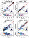 |
Fig. 5. Model predicted fexsitu vs. the ground truth. The different panels are models trained and validated by TNG100 and EAGLE in the top, and cross-validated with each other in the bottom, all with the combined parameters Sub0. For each column we show the one-to-one comparison in the top panel: r is |

In all the models there is a slight systematic bias that the models tend to overpredict fexsitu for those galaxies with low fexsitu, and underpredict fexsitu for the few galaxies with very high fexsitu. The standard derivation of Δfexsitu is almost constant, with 0.1 across fexsitu.
We further check how well the models reproduce fexsitu as a function of galaxy stellar mass in Fig. 6. The models, either trained by TNG100 or EAGLE, reproduce well the fexsitu as a function of stellar mass for both TNG100 and EAGLE galaxies, including the medium curve and the 1σ scatter. There is no systematic bias as a function of galaxy stellar mass, except for the most massive galaxies at M* ≳ 5 × 10¹¹ M⊙ where we have very few galaxies in both the training and validation data sets.
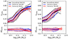 |
Fig. 6. fexsitu as a function of stellar mass for model predications vs. ground truth. In the left panel the black solid curve is the median of the ground truth for the TNG100 galaxies; the blue and red solid curves represent those predicted by Model A (trained by TNG100) and Model C (trained by EAGLE); and the dashed curves are the ±1σ scatter. In the right panel the black curves are the ground truth for EAGLE galaxies; the blue and red represent those predicted by Model B (trained by EAGLE) and Model D (trained by TNG100). |
5. Discussion
5.1. The effects of observational noise
We used mock images with SDSS-like observational data and placed galaxies at 40 Mpc in the above analysis. To understand how the results are affected by the observational noise, we created a few versions of mock images from TNG100 by placing the galaxies at 40, 200, 400, and 600 Mpc with the SDSS-like observational noise and placing the galaxies at 40, 200, 400, 600, 1000, and 1500 Mpc with HSC-like observational noise. In comparison, we also created a version of clean image placing at 40 Mpc and without observational noise.
We extracted similar parameters from these mock images, and show the correlations between the photometric parameters and fexsitu in Figs. 7 and 8. We focus on the six parameters that are of the highest importance in predicting fexsitu here (i.e. the parameters in Sub0).
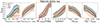 |
Fig. 7. Parameters derived from mock images vs. fexsitu for galaxies placed at different distances and with SDSS-like observations. In each panel the black curve represents galaxies at 40 Mpc and without observational noise; the blue, green, yellow, and red curves represent galaxies with observational noise and placed at 40, 200, 400, and 600, respectively. The solid curves are running median and the dashed curves are ±1σ scatter. |
For the galaxies with SDSS-like observational noise shown in Fig. 7, we see that the correlations of finnerhalo versus fexsitu are identical for galaxies at 40 Mpc with or without observational noise, and still the same when the galaxies are placed at 200 Mpc. However, it shows deviations for galaxies at larger distances (400 Mpc or 600 Mpc). The inner stellar halos are contaminated by disks with PSF convolution. The luminosity fraction of the disk has a negative correlation with fexsitu, and thus contamination by the disk could significantly diminish the ability to predict fexsitu for the inner stellar halo.
There is an offset in the correlation of fouterhalo versus fexsitu between those created from images with and without observation noise, while the correlations for galaxies with noise at 40–600 Mpc are similar. The luminosity of the outer halo is affected by the background noise; the good thing is that the effects of noise are stable for galaxies at different distances (here 40–600 Mpc). The other importance parameters, including ∇ρouter, ∇(g − r)outer, Mr, and size r90 are less affected by observational noise, and the correlations with fexsitu are identical for galaxies at d ≲ 400 Mpc, with or without observational noise.
We imposed a smaller PSF kernel and lower background noise for HSC-like mock images than for SDSS-like images. As shown in Fig. 8, with HSC-like observations, the correlation of finnerhalo versus fexsitu starts to deviate from the original for galaxies with d ≳ 400 Mpc. The correlation between fexsitu and the other important parameters remains unchanged for galaxies with d ≲ 1000 Mpc, and some of them, ∇ρouter versus fexsitu and ∇(g − r)outer versus fexsitu, begin to deviate from the original for galaxies at d = 1500 Mpc.
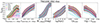 |
Fig. 8. Same as Fig. 7, but for galaxies with HSC-like observations. In each panel the black curve represents galaxies at 40 Mpc and without observational noise; the blue, green, yellow, red, magenta, and cyan curves represent galaxies with observational noise and placed at 40, 200, 400, 600, 1000, and 1500 Mpc, respectively. |
The inner halo luminosity finnerhalo is easily affected by PSF, and thus is sensitive to the galaxy distance. Our above model including finnerhalo is thus only capable for SDSS-like galaxies at d ≲ 200 Mpc and HSC-like galaxies at d ≲ 400 Mpc.
We created a new random forest model with the combination of parameters Sub1 that are less affected by the galaxy distance: ∇ρouter and ∇(g − r)outer, fouterhalo, Mr, r90, excluding finnerhalo from Sub0. We trained the model with 70% of the galaxies at 40 Mpc, and made predictions for the other 30% of the galaxies, but put at further distances. In Fig. 9 we show the standard deviation of the model residuals (σ(Δfexsitu)) for SDSS-like and HSC-like galaxies at difference distances.
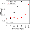 |
Fig. 9. Standard deviation of model residuals, σ(Δfexsitu), with a model trained with galaxies at 40 Mpc and tested with mock galaxies put at different distances, as shown along the x-axis. The red points are HSC-like galaxies, and the black points are SDSS-like galaxies. |
For galaxies at 40 Mpc, the residual σ(Δfexsitu) of the Sub1 model is similar to that of the model trained by Sub0 that includes finnerhalo. The surface brightness gradients ∇ρouter contain information similar to finnerhalo and fouterhalo, but are less affected by PSF. The residual of the model increases with the galaxy distance, but it still remains σ(Δfexsitu)≲0.1 for SDSS-like galaxies at r ≲ 400 Mpc (z ≲ 0.1) and for HSC-like galaxies at r ≲ 1000 Mpc (z ≲ 0.2). Our model trained by the Sub1 parameters should be valid for galaxies in these regions. Future large surveys such as Legacy Survey of Space and Time (LSST) and China Space Station Telescope (CSST) will observe a large sample of galaxies with high data quality, which will likely allow us to apply the model to galaxies at larger distances.
5.2. Advantages and caveats
We summarise our model performance in Table 4 for the four sets of models trained and validated by the TNG100 and EAGLE galaxies, and those that were cross-validated. We have model residuals of σ(Δfexsitu) = 0.08 − 0.09. There are a few works in the literature that try to obtain galaxies’ ex situ stellar mass fraction through the machine learning method. We make a comparison with their results in Table 4.
Model performance compared with previous works.
Most of the parameters used in Shi et al. (2022) are defined from mock photometric images similar to ours, including Mr, Mg, r90, r50, g − r, and concentration C. They included these parameters, as well as the total stellar mass M* and the single aperture velocity dispersion σ to train a random forest model. In their model, the most important parameters are the total stellar mass M* and the size r90. Although they included M* as the input parameter, they still have σ(Δfexsitu)∼0.1, which is slightly larger than for our model trained and validated by the same TNG100 galaxies. A better prediction with σ(Δfexsitu)∼0.06 is obtained by a cINN model from Eisert et al. (2023). However, they included some parameters that cannot be directly derived from photometric data and potentially could have a large uncertainty for real observations. The parameters they used include the total stellar mass, M*; the lookback time of the galaxy; the half-light radius, Re; the dynamically defined disk fraction, fdisk; the luminosity-weighted stellar age, Age*; and the metallicity, Z*.
The above models were created by TNG100 galaxies and were not cross-validated by other simulations. There is a CNN model using 2D maps of stellar mass, stellar velocity, velocity dispersion, stellar age, and metallicity that makes good predictions of fexsitu with a scatter of ∼0.07 when trained and validated by the same TNG100 galaxies and that was cross-validated by the TNG100 and EAGLE galaxies (Angeloudi et al. 2023). However, the input data used in this model can only be obtained from expensive IFU data.
Our model using only parameters defined from photometric data works similarly well to other models in the literature employing parameters that need spectroscopic observations or that are potentially harder to obtain. The luminosity fractions of the inner and outer halo (finnerhalo and fouterhalo), or equivalently the surface brightness and colour gradients (∇ρouter and ∇(g − r)outer)) we defined, play crucial importance here.
As any other models trained by simulations, our model could depend on the galaxy formation model and the resolution of the simulations. We cross-validated the model between TNG100, EAGLE, and also TNG50 (see Figures B.1 and B.2), which show that our model generally converges among these different simulations. However, the model prediction for some special type of galaxies could still be affected by the limited galaxy populations of the simulation. For example, EAGLE lacks galaxies with fexsitu > 0.7, and thus there is an upper limit of fexsitu for TNG100 galaxies predicted by the EAGLE trained model as shown in the bottom left panel of Fig. 5.
A major limitation of our model is that it is only capable for edge-on galaxies. On the one hand, the definitions of edge-on galaxies from observations and simulations are different. When applying the model to observations, it is hard to have a sample of galaxies perfectly edge-on, as theoretically defined. In the Appendix, we show that our results are affected, but not so significantly, by the inclination angle. For a sample of edge-on galaxies mixed with the 20% of the galaxies that are moderately inclined, our model still works statistically well. On the other hand, we lost a large fraction of real galaxies not edge-on. For these galaxies not edge-on, the contamination of the disk will dilute the correlations and weaken the power of our model in predicting fexsitu. Potentially, the disk could be removed by photometric decomposition. However, photometric disk and bulge decomposition has not worked well for simulated galaxies (Rodriguez-Gomez et al. 2019), it may not lead to consistent results with real observations. We may further validate the method by trying photometric decomposition to observed non-edge-on galaxies, and comparing these results with the results from edge-on galaxies.
6. Conclusion
We created mock images using galaxies in the cosmological hydrodynamical simulations TNG100, EAGLE, and TNG50 at redshift z = 0. We projected all galaxies as edge-on, and defined a series of parameters describing their structures, including the absolute magnitude in r and g bands (Mr, Mg), the half-light and 90%-light radius (r50, r90), the concentration (C), the luminosity fractions of inner and outer halos (finnerhalo, fouterhalo), the inner and outer surface brightness gradient (∇ρinner and ∇ρouter), colour gradients (∇(g − r)inner and ∇(g − r)outer), and the single-aperture velocity dispersion (σ) and Kurtosis from Gaussian-Hermit fitting (h4).
In particular, the inner and outer halo of a galaxy are defined by a sector along the minor axis, with 45 − 135 degrees from the disk major axis, and with radii ranging from 3.5 to 10 kpc and 10–30 kpc, respectively, to avoid contamination of the disk and bulge. The surface brightness and the colour gradients are defined in the same sector along the minor axis, and in radii ranges of 1.5–10 kpc and 10–30 kpc for the inner and outer gradients, respectively. We then evaluated the importance of these parameters in predicting the ex situ stellar mass fraction, fexsitu, and constructed machine learning models using the random forest(random forest) method to predict fexsitu.
Our main results are as follows:
-
We find that the outer gradients of surface brightness (∇ρouter) and colour (∇(g − r)outer), as well as the luminosity fraction of the inner and outer halo (finnerhalo and fouterhalo) are strongly correlated with the ex situ stellar mass fraction fexsitu, and these correlations are almost identical in TNG100, EAGLE, and TNG50, independently of the galaxy formation model and simulation resolution used.
-
We evaluate the importance of all structure parameters in predicting the ex situ stellar mass fraction (fexsitu). We find that the parameters of highest importance in the model are ∇ρouter, ∇(g − r)outer, fouterhalo, and finnerhalo, followed by the absolute magnitude Mr and the galaxy size r90; the remaining parameters are not important.
-
We trained the random forest models by including the six most important parameters (Sub0: ∇ρouter, ∇(g−r)outer, fouterhalo, finnerhalo, Mr, r90) measured from mock photometric images: the models effectively predict the ex situ fraction with residual σ(Δfexsitu) < 0.1. The models trained from TNG100 and EAGLE work similarly well and are cross-validated; they also work well in making predictions for TNG50 galaxies.
-
The correlations of ∇ρouter versus fexsitu, ∇(g − r)outer versus fexsitu and fouterhalo versus fexsitu are affected by observational noise, but remain unchanged for galaxies with d ≲ 400 Mpc (z ≲ 0.1) for SDSS-like observations and d ≲ 1000 Mpc (z ≲ 0.2) for HSC-like observations. Our model is thus validated for galaxies with such data quality and within these distances.
In summary, the luminosity and colour gradients, as well as the luminosity fraction of the inner and outer halo, can robustly predict the ex situ stellar mass fraction in nearby galaxies. The correlations between these parameters and fexsitu are almost identical in all the simulations we explored. Our models trained by random forest can be transferred between TNG100, EAGLE, and TNG50 galaxies, and thus could potentially be applied to real galaxies from large photometric surveys.
Acknowledgments
The authors thank Song Huang for useful discussions. LZ acknowledges the support of the National Key R&D Programme of China No. 2022YFF0503403, and the CAS Project for Young Scientists in Basic Research under grant No. YSBR-062. WW acknowledge the support of NSFC (12273021), the National Key R&D Programme of China (2023YFA1605600, 2023YFA1605601) and the Yangyang Development Fund. JF-B acknowledges support from the PID2022-140869NB-I00 grant from the Spanish Ministry of Science and Innovation.
References
- Abdurro’uf, Accetta, K., Aerts, C., et al. 2022, ApJS, 259, 35 [NASA ADS] [CrossRef] [Google Scholar]
- Aihara, H., AlSayyad, Y., Ando, M., et al. 2022, PASJ, 74, 247 [NASA ADS] [CrossRef] [Google Scholar]
- Angeloudi, E., Falcón-Barroso, J., Huertas-Company, M., et al. 2023, MNRAS, 523, 5408 [CrossRef] [Google Scholar]
- Angeloudi, E., Falcón-Barroso, J., Huertas-Company, M., et al. 2024, Nature Astronomy, 8, 1310 [Google Scholar]
- Bacon, R., Copin, Y., Monnet, G., et al. 2001, MNRAS, 326, 23 [Google Scholar]
- Belokurov, V., Erkal, D., Evans, N. W., Koposov, S. E., & Deason, A. J. 2018, MNRAS, 478, 611 [Google Scholar]
- Boecker, A., Leaman, R., van de Ven, G., et al. 2020, MNRAS, 491, 823 [Google Scholar]
- Bois, M., Bournaud, F., Emsellem, E., et al. 2010, MNRAS, 406, 2405 [NASA ADS] [CrossRef] [Google Scholar]
- Bois, M., Emsellem, E., Bournaud, F., et al. 2011, MNRAS, 416, 1654 [Google Scholar]
- Breiman, L. 2001, Machine Learning, 45, 5 [NASA ADS] [CrossRef] [Google Scholar]
- Breiman, L., Friedman, J. H., Olshen, R. A., & Stone, C. J. 1984, Classification and Regression Trees [Google Scholar]
- Bundy, K., Bershady, M. A., Law, D. R., et al. 2015, ApJ, 798, 7 [Google Scholar]
- Conselice, C. J. 2003, ApJS, 147, 1 [NASA ADS] [CrossRef] [Google Scholar]
- Cooper, A. P., D’Souza, R., Kauffmann, G., et al. 2013, MNRAS, 434, 3348 [Google Scholar]
- Cooper, A. P., Gao, L., Guo, Q., et al. 2015, MNRAS, 451, 2703 [Google Scholar]
- Crain, R. A., Schaye, J., Bower, R. G., et al. 2015, MNRAS, 450, 1937 [NASA ADS] [CrossRef] [Google Scholar]
- Croom, S. M., Lawrence, J. S., Bland-Hawthorn, J., et al. 2012, MNRAS, 421, 872 [NASA ADS] [Google Scholar]
- Das, P., Hawkins, K., & Jofré, P. 2020, MNRAS, 493, 5195 [NASA ADS] [CrossRef] [Google Scholar]
- Davison, T. A., Kuntschner, H., Husemann, B., et al. 2021a, MNRAS, 502, 2296 [NASA ADS] [CrossRef] [Google Scholar]
- Davison, T. A., Norris, M. A., Leaman, R., et al. 2021b, MNRAS, 507, 3089 [NASA ADS] [CrossRef] [Google Scholar]
- D’Souza, R., Kauffman, G., Wang, J., & Vegetti, S. 2014, MNRAS, 443, 1433 [Google Scholar]
- Eisert, L., Pillepich, A., Nelson, D., et al. 2023, MNRAS, 519, 2199 [Google Scholar]
- Emsellem, E., Cappellari, M., Krajnović, D., et al. 2011, MNRAS, 414, 888 [Google Scholar]
- Fall, S. M., & Efstathiou, G. 1980, MNRAS, 193, 189 [NASA ADS] [CrossRef] [Google Scholar]
- Forbes, D. A., & Remus, R.-S. 2018, MNRAS, 479, 4760 [Google Scholar]
- Genel, S., Nelson, D., Pillepich, A., et al. 2018, MNRAS, 474, 3976 [Google Scholar]
- Gerhard, O. E. 1993, MNRAS, 265, 213 [Google Scholar]
- Helmi, A., Babusiaux, C., Koppelman, H. H., et al. 2018, Nature, 563, 85 [Google Scholar]
- Hilz, M., Naab, T., Ostriker, J. P., et al. 2012, MNRAS, 425, 3119 [Google Scholar]
- Huang, S., Ho, L. C., Peng, C. Y., Li, Z.-Y., & Barth, A. J. 2013, ApJ, 766, 47 [Google Scholar]
- Hubble, E. P. 1926, ApJ, 64, 321 [Google Scholar]
- Kormendy, J., & Kennicutt, R. C., Jr 2004, ARA&A, 42, 603 [NASA ADS] [CrossRef] [Google Scholar]
- Kruijssen, J. M. D., Pfeffer, J. L., Chevance, M., et al. 2020, MNRAS, 498, 2472 [NASA ADS] [CrossRef] [Google Scholar]
- Lange, R., Moffett, A. J., Driver, S. P., et al. 2016, MNRAS, 462, 1470 [NASA ADS] [CrossRef] [Google Scholar]
- Marinacci, F., Vogelsberger, M., Pakmor, R., et al. 2018, MNRAS, 480, 5113 [NASA ADS] [Google Scholar]
- Martig, M., Pinna, F., Falcón-Barroso, J., et al. 2021, MNRAS, 508, 2458 [NASA ADS] [CrossRef] [Google Scholar]
- McAlpine, S., Helly, J. C., Schaller, M., et al. 2016, Astronomy and Computing, 15, 72 [NASA ADS] [CrossRef] [Google Scholar]
- Monaghan, J. J. 1992, ARA&A, 30, 543 [NASA ADS] [CrossRef] [Google Scholar]
- Monaghan, J. J., & Lattanzio, J. C. 1985, A&A, 149, 135 [NASA ADS] [Google Scholar]
- Naiman, J. P., Pillepich, A., Springel, V., et al. 2018, MNRAS, 477, 1206 [Google Scholar]
- Nelson, D., Pillepich, A., Springel, V., et al. 2018, MNRAS, 475, 624 [Google Scholar]
- Nelson, D., Pillepich, A., Springel, V., et al. 2019a, MNRAS, 490, 3234 [Google Scholar]
- Nelson, D., Springel, V., Pillepich, A., et al. 2019b, Computational Astrophysics and Cosmology, 6, 2 [CrossRef] [Google Scholar]
- Nelson, E. J., Tacchella, S., Diemer, B., et al. 2021, MNRAS, 508, 219 [NASA ADS] [CrossRef] [Google Scholar]
- Pedregosa, F., Varoquaux, G., Gramfort, A., et al. 2011, Journal of Machine Learning Research, 12, 2825 [Google Scholar]
- Pillepich, A., Madau, P., & Mayer, L. 2015, ApJ, 799, 184 [Google Scholar]
- Pillepich, A., Springel, V., Nelson, D., et al. 2018, MNRAS, 473, 4077 [Google Scholar]
- Pillepich, A., Nelson, D., Springel, V., et al. 2019, MNRAS, 490, 3196 [Google Scholar]
- Pinna, F., Falcón-Barroso, J., Martig, M., et al. 2019a, A&A, 625, A95 [NASA ADS] [CrossRef] [EDP Sciences] [Google Scholar]
- Pinna, F., Falcón-Barroso, J., Martig, M., et al. 2019b, A&A, 623, A19 [NASA ADS] [CrossRef] [EDP Sciences] [Google Scholar]
- Pulsoni, C., Gerhard, O., Arnaboldi, M., et al. 2020, A&A, 641, A60 [EDP Sciences] [Google Scholar]
- Remus, R.-S., & Forbes, D. A. 2022, ApJ, 935, 37 [NASA ADS] [CrossRef] [Google Scholar]
- Rodriguez-Gomez, V., Pillepich, A., Sales, L. V., et al. 2016, MNRAS, 458, 2371 [Google Scholar]
- Rodriguez-Gomez, V., Sales, L. V., Genel, S., et al. 2017, MNRAS, 467, 3083 [Google Scholar]
- Rodriguez-Gomez, V., Snyder, G. F., Lotz, J. M., et al. 2019, MNRAS, 483, 4140 [NASA ADS] [CrossRef] [Google Scholar]
- Sánchez, S. F., Kennicutt, R. C., Gil de Paz, A., et al. 2012, A&A, 538, A8 [Google Scholar]
- Schaye, J., Crain, R. A., Bower, R. G., et al. 2015, MNRAS, 446, 521 [Google Scholar]
- Shi, R., Wang, W., Li, Z., et al. 2022, MNRAS, 515, 3938 [CrossRef] [Google Scholar]
- Spavone, M., Capaccioli, M., Napolitano, N. R., et al. 2017, A&A, 603, A38 [NASA ADS] [CrossRef] [EDP Sciences] [Google Scholar]
- Spavone, M., Iodice, E., van de Ven, G., et al. 2020, A&A, 639, A14 [NASA ADS] [CrossRef] [EDP Sciences] [Google Scholar]
- Springel, V., Pakmor, R., Pillepich, A., et al. 2018, MNRAS, 475, 676 [Google Scholar]
- Stoughton, C., Lupton, R. H., Bernardi, M., et al. 2002, AJ, 123, 485 [Google Scholar]
- Tacchella, S., Diemer, B., Hernquist, L., et al. 2019, MNRAS, 487, 5416 [Google Scholar]
- Toomre, A. 1977, in Evolution of Galaxies and Stellar Populations, eds. B. M. Tinsley, D. C. Larson, & R. B. Gehret, 401 [Google Scholar]
- Trayford, J. W., Frenk, C. S., Theuns, T., Schaye, J., & Correa, C. 2019, MNRAS, 483, 744 [NASA ADS] [CrossRef] [Google Scholar]
- van der Marel, R. P., & Franx, M. 1993, ApJ, 407, 525 [Google Scholar]
- Walcher, C., Wisotzki, L., Bekeraité, S., et al. 2014, Journal of Astrophysics and Astronomy, 569 [Google Scholar]
- Xu, D., Zhu, L., Grand, R., et al. 2019, MNRAS, 489, 842 [NASA ADS] [CrossRef] [Google Scholar]
- Zhu, L., van de Ven, G., Leaman, R., et al. 2020, MNRAS, 496, 1579 [Google Scholar]
- Zhu, L., Pillepich, A., van de Ven, G., et al. 2022a, A&A, 660, A20 [NASA ADS] [CrossRef] [EDP Sciences] [Google Scholar]
- Zhu, L., van de Ven, G., Leaman, R., et al. 2022b, A&A, 664, A115 [NASA ADS] [CrossRef] [EDP Sciences] [Google Scholar]
Appendix A: Galaxies with ongoing mergers
We checked all the SDSS-like mock images by eye, and identify these galaxies with obvious substructures in the inner halo or with disk obviously disturbed as ongoing merging galaxies. These galaxies are excluded from our sample. We show six of these cases in Fig.A.1.
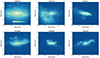 |
Fig. A.1. Six cases of galaxies with ongoing mergers, with their subhalo ID labelled at the top. |
Appendix B: Model prediction for TNG50 galaxies
In Figure B.1, we show that the TNG50 galaxies have trends similar to those of TNG100 and EAGLE in the correlations of finnerhalo, fouterhalo, ∇ρouter and ∇(g − r)outer versus fexsitu, and they have obvious offsets with TNG100 and EAGLE in the other correlations. The parameters finnerhalo, fouterhalo, ∇ρouter and ∇(g − r)outer are probably not affected by simulation resolutions.
To further check if the simulation resolution will affect our results, we use the models trained by the mock data created from TNG100 and EAGLE, and make predictions for TNG50 galaxies. We show the model prediction versus the ground truth of fexsitu in Figure B.2, the models work well with σ(Δ(fexsitu)) = 0.08. Our model probably already converges at the resolution of TNG100.
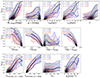 |
Fig. B.1. Correlation of ex situ stellar mass fraction fexsitu with morphological parameters. The figure is similar to Figure 3, but with the morphological parameters derived from the clean images without observational noise. The black, blue, and red solid curves are running median for TNG100, EAGLE, and TNG50 galaxies; the dashed curves represent the ±σ scatter. |
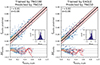 |
Fig. B.2. Model predictions vs. ground truth, similar to Fig.5, but making predictions for TNG50 galaxies with clean images. |
Appendix C: The effects of inclination angle on the model prediction
We limited our model to edge-on galaxies in the paper. However, the definitions of edge-on galaxies from observations and simulations are different. When applying the model to observations, it is hard to have a sample of galaxies perfectly edge-on, as theoretically defined. Here we evaluate how the results will be affected if the sample is mixed with some galaxies not perfectly edge-on.
We used the model trained by TNG100 edge-on galaxies shown in the paper (inclination angle i = 80o − 90o), and made predictions for a sample composed of 80% galaxies with i = 80o − 90o and mixed with 20% with i = 60o − 80o. In Figure C.1, we show the model prediction versus ground truth. The model works statistically well for the mixed sample, with ℛ = 0.87 and the standard deviation of σ(Δ(fexsitu)) = 0.09, similar to the model prediction for all edge-on galaxies.
We also trained and validated a model using TNG100 galaxies randomly projected between i = 0o − 90o. As shown in the right panel of Figure C.1, the model works less well compared to that limited to edge-on galaxies. Especially for the disk galaxies with low ex situ stellar mass, the model tends to over-predict their ex situ stellar mass fractions.
 |
Fig. C.1. Model predictions vs. ground truth, similar to Fig. 5. Left panel: Model trained by TNG100 galaxies with i = 80o − 90o, but making prediction for a sample composed of 80% galaxies with i = 80o − 90o and mixed with 20% with i = 60o − 80o. Right panel: Model trained and validated by TNG100 galaxies randomly projected between i = 0o − 90o. |
All Tables
Basic information regarding the publicly available cosmological simulations we use or refer to in this paper.
All Figures
|
Fig. 1. Galaxy stellar mass–size relation of simulations analysed in this paper: (from left to right) TNG100, EAGLE, and TNG50. We chose the stellar mass, M*, defined within a spherical radius of 30 kpc vs. r50 defined from a 2D image. The galaxies kept in our analysis with M* > 1010.3 M⊙ are coloured in blue, the galaxies with ongoing mergers are removed from our analysis and are coloured in grey. |
| In the text | |
|
Fig. 2. SDSS-like r-band image created from a TNG100 galaxy subhalo 6 at z = 0 projected near edge-on, and placed at the distance of 40 Mpc. Top: 2D image. The sector enclosed by blue is defined as the inner halo (3.5 kpc–10 kpc) and that in red as the outer halo (10 kpc–30 kpc). Bottom: surface brightness profile along the minor axis. The black horizontal line indicates the background noise of the sky Σr, 0; the red and magenta vertical lines mark r50 and r90 obtained from the Petrosian radius. |
| In the text | |
|
Fig. 3. Correlations between the parameters extracted from mock SDSS photometric observations for galaxies at 40 Mpc and the ex situ stellar mass fraction of galaxies. The grey dots are TNG100 galaxies; the black solid and dashed curves are the running median and the ±1σ scatter of the TNG100 galaxies. The blue symbols are for EAGLE galaxies. The Spearman’s rank coefficient(ρ) of each correlation is labelled in the figure. |
| In the text | |
|
Fig. 4. Importance (r2) of the observational parameters in predicting the ex situ stellar mass fraction fexsitu. The top panels are models trained and validated by TNG100 and EAGLE, respectively; the bottom panels are models cross-validated with TNG100 and EAGLE. In each panel the two black points shows the importance of combined parameters: Sub0 including ∇ρouter, ∇(g − r)outer, fouterhalo, finnerhalo, Mr, r90; Sub1 including the same, but not finnerhalo. The rest of the points show the importance of each single parameter as labelled. The error bars in the top two panels are the scatter of results from different training and validating sets and different hyperparameters of the random forest models; the error bars in the bottom two panels are from different hyperparameters of the random forest models. |
| In the text | |
|
Fig. 5. Model predicted fexsitu vs. the ground truth. The different panels are models trained and validated by TNG100 and EAGLE in the top, and cross-validated with each other in the bottom, all with the combined parameters Sub0. For each column we show the one-to-one comparison in the top panel: r is |
| In the text | |
|
Fig. 6. fexsitu as a function of stellar mass for model predications vs. ground truth. In the left panel the black solid curve is the median of the ground truth for the TNG100 galaxies; the blue and red solid curves represent those predicted by Model A (trained by TNG100) and Model C (trained by EAGLE); and the dashed curves are the ±1σ scatter. In the right panel the black curves are the ground truth for EAGLE galaxies; the blue and red represent those predicted by Model B (trained by EAGLE) and Model D (trained by TNG100). |
| In the text | |
|
Fig. 7. Parameters derived from mock images vs. fexsitu for galaxies placed at different distances and with SDSS-like observations. In each panel the black curve represents galaxies at 40 Mpc and without observational noise; the blue, green, yellow, and red curves represent galaxies with observational noise and placed at 40, 200, 400, and 600, respectively. The solid curves are running median and the dashed curves are ±1σ scatter. |
| In the text | |
|
Fig. 8. Same as Fig. 7, but for galaxies with HSC-like observations. In each panel the black curve represents galaxies at 40 Mpc and without observational noise; the blue, green, yellow, red, magenta, and cyan curves represent galaxies with observational noise and placed at 40, 200, 400, 600, 1000, and 1500 Mpc, respectively. |
| In the text | |
|
Fig. 9. Standard deviation of model residuals, σ(Δfexsitu), with a model trained with galaxies at 40 Mpc and tested with mock galaxies put at different distances, as shown along the x-axis. The red points are HSC-like galaxies, and the black points are SDSS-like galaxies. |
| In the text | |
|
Fig. A.1. Six cases of galaxies with ongoing mergers, with their subhalo ID labelled at the top. |
| In the text | |
|
Fig. B.1. Correlation of ex situ stellar mass fraction fexsitu with morphological parameters. The figure is similar to Figure 3, but with the morphological parameters derived from the clean images without observational noise. The black, blue, and red solid curves are running median for TNG100, EAGLE, and TNG50 galaxies; the dashed curves represent the ±σ scatter. |
| In the text | |
|
Fig. B.2. Model predictions vs. ground truth, similar to Fig.5, but making predictions for TNG50 galaxies with clean images. |
| In the text | |
|
Fig. C.1. Model predictions vs. ground truth, similar to Fig. 5. Left panel: Model trained by TNG100 galaxies with i = 80o − 90o, but making prediction for a sample composed of 80% galaxies with i = 80o − 90o and mixed with 20% with i = 60o − 80o. Right panel: Model trained and validated by TNG100 galaxies randomly projected between i = 0o − 90o. |
| In the text | |
Current usage metrics show cumulative count of Article Views (full-text article views including HTML views, PDF and ePub downloads, according to the available data) and Abstracts Views on Vision4Press platform.
Data correspond to usage on the plateform after 2015. The current usage metrics is available 48-96 hours after online publication and is updated daily on week days.
Initial download of the metrics may take a while.