| Issue |
A&A
Volume 695, March 2025
|
|
|---|---|---|
| Article Number | A24 | |
| Number of page(s) | 17 | |
| Section | Interstellar and circumstellar matter | |
| DOI | https://doi.org/10.1051/0004-6361/202452371 | |
| Published online | 28 February 2025 | |
ATLASGAL-selected high-mass clumps in the inner Galaxy
XI. Morphology and kinematics of warm inner envelopes
1
Max-Planck-Institut für Radioastronomie,
Auf dem Hügel 69,
53121
Bonn,
Germany
2
Korea Astronomy and Space Science Institute,
776 Daedeok-daero, Yuseong-gu,
Daejeon
34055,
Republic of Korea
3
Department of Astronomy and Space Science, University of Science and Technology,
217 Gajeong-ro,
Daejeon
34113,
Republic of Korea
4
Argelander-Institut für Astronomie, Universität Bonn,
Auf dem Hügel 71,
53121
Bonn,
Germany
5
Institute of Astronomy, Faculty of Physics, Astronomy and Informatics, Nicolaus Copernicus University,
ul. Grudziądzka 5,
87-100
Toruń,
Poland
6
SOAR Telescope/NSF’s NOIRLab,
Avda Juan Cisternas 1500,
1700000
La Serena,
Chile
★★ Corresponding author; tdhoang@mpifr-bonn.mpg.de
Received:
26
September
2024
Accepted:
22
January
2025
Context. High-mass stellar embryos are embedded in warm envelopes that provide mass reservoirs for the accretion process onto final stars. Feedback from star formation activities in return impacts the properties of the envelopes, offering us a unique opportunity to investigate star formation processes.
Aims. Our goals are to characterise the properties of warm envelopes of proto- or young stellar objects at different evolutionary stages based on the morphology and kinematics of submillimetre emission from the 13CO (6–5) line and to examine their relations with star formation processes.
Methods. Using the Atacama Pathfinder EXperiment (APEX) telescope, we obtained maps of 13CO (6–5) emission with an angular size of 80″ × 80″ (ranging from 0.3 pc × 0.3 pc to 4.9 pc × 4.9 pc in physical size) of 99 massive clumps from the ATLASGAL survey of submillimetre dust continuum emission. Our maps are classified based on morphological complexities, and the radial structure of 13CO (6–5) emission is characterised for simple single-core sources. In addition, the velocity centroids of 13CO (6–5) emission are compared to small- and large-scale gas kinematics (traced by 12CO (6–5) and 13CO (2–1) emission, respectively), aiming to shed light on the origin of envelope kinematics.
Results. 13CO (6–5) emission is detected towards sources in all stages of high-mass star formation, with a detection rate of 83% for the whole sample. The detection rate, line width, and peak brightness temperature increase with evolutionary stage, and the line luminosity is strongly correlated with the bolometric luminosity and the clump mass. These results indicate that the excitation of 13CO (6–5) emission is closely related to star formation processes. In addition, the radial distributions of 13CO (6–5) emission for single-core sources can be well fitted by power-law functions, suggesting a relatively simple envelope structure for the majority of our sources (52 out of 99). The slopes of the radial distributions are systematically steeper for the most evolved group of sources (that host HII regions), which likely results from enhancements in density and/or temperature at the central parts of the warm envelopes. As for the 13CO (6–5) kinematics, linear velocity gradients are common among the single-core sources (44 out of 52), and the measured mean velocity gradients are on average 3 km s−1 pc−1. Our comparison of the 13CO (6−5), 12CO (6−5), and 13CO(2−1) kinematics suggests that the origin of the linear velocity gradients in the warm envelopes is complex and unclear for many sources.
Conclusions. 13CO (6–5) emission is ubiquitous in a wide variety of massive clumps, ranging from young sources where protostars have not yet been formed to evolved sources with fully developed HII regions. The excitation of 13CO (6–5) emission in warm envelopes is likely impacted by different processes at different epochs of high-mass star formation, while the origin of the 13CO (6–5) kinematics remains elusive and needs further investigation.
Key words: stars: formation / stars: massive / stars: protostars / ISM: kinematics and dynamics / ISM: molecules / ISM: structure
© The Authors 2025
 Open Access article, published by EDP Sciences, under the terms of the Creative Commons Attribution License (https://creativecommons.org/licenses/by/4.0), which permits unrestricted use, distribution, and reproduction in any medium, provided the original work is properly cited.
This article is published in open access under the Subscribe to Open model.
Open Access funding provided by Max Planck Society.
1 Introduction
High-mass stars (M > 8 M⊙) play an essential role in the evolution of galaxies (e.g. Kennicutt 2005). They provide a substantial amount of radiative and mechanical feedback to the surrounding interstellar medium (ISM) through ultraviolet (UV) radiation fields, stellar outflows, stellar winds, and supernova explosions, regulating star formation in galaxies (Hopkins et al. 2014). In addition, they produce and release heavy elements throughout their lifetime, driving the chemical enrichment of galaxies (Matteucci 2021).
Despite their importance for the evolution of galaxies, how high-mass stars form and interact with their surroundings remains poorly understood (e.g. Zinnecker & Yorke 2007; Motte et al. 2018). Current competing theoretical concepts of high-mass star formation include collapsing turbulent cores (McKee & Tan 2003), competitive accretion in stellar clusters (Bonnell et al. 2001; Bonnell & Bate 2006), global hierarchical collapse (Vázquez-Semadeni et al. 2019), and converging inertial flows (Padoan et al. 2020). Evaluating these different theories rigorously requires a statistically significant sample of high-mass star-forming regions, covering a wide range of evolutionary stages. Such a sample has been provided by the APEX Telescope Large Area Survey of the Galaxy (ATLASGAL; Schuller et al. 2009). ATLASGAL is a survey of 870 µm emission in the inner Galaxy (covering |l| < 60° at |b| < 1.5° and 280° < l < 300° at −2° < b < 1°) conducted with the Atacama Pathfinder EXperiment (APEX1; Güsten et al. 2006) 12 m submillimetre telescope in Chile. With an excellent sensitivity of 50–70 mJy beam−1 and a large coverage of ~420 deg2, ATLASGAL provides a comprehensive census of high-mass star-forming regions in the inner Galaxy.
Within high-mass star-forming regions, dense envelopes are of particular interest as they provide mass reservoirs that feed the mass build-up of newly formed protostellar objects at their centres through accretion (Shu et al. 1987; Wyrowski et al. 2016; Beltrán & de Wit 2016; Pillai et al. 2023). Once young stellar objects (YSOs) have formed, stellar feedback significantly changes the properties of the surrounding envelopes, so much so that they can be entirely dispersed at the end of the evolution, stopping the accretion process (e.g. Arce & Sargent 2006, for low-mass star-forming regions). Among other tracers, mid-J (5 < J < 10) rotational transitions of isotopologues of carbon monoxide (CO) are especially suitable for probing the warm (T ≳ 50 K) inner parts of the envelopes. Previous studies have suggested that the warm envelopes surrounding low- and high- mass YSOs can be heated by various physical processes that are related to star formation activities. For example, passive heating and UV radiation from outflow cavity walls have been proposed to explain13 CO (6−5) emission in low-mass star-forming regions (van Kempen et al. 2009b; Yıldız et al. 2012). Similarly, UV photons from photodissociation regions (PDRs) have been shown to play an important role in the excitation of 13CO (6−5) emission in several high-mass star-forming clumps with strong H II regions (Graf et al. 1993; Koester et al. 1994; Leurini et al. 2013).
While there have certainly been a number of dedicated studies of the warm envelopes, mid-J transitions of CO isotopologues still remain difficult to access observationally due to the required dry atmospheric conditions. In particular, there is a lack of studies that cross a wide range of high-mass starforming regions (including those in the early stages before the development of HII regions). In this paper, we examine the properties of 13CO (6−5)-traced warm envelopes for a sample of 99 ATLASGAL-selected high-mass star-forming regions based on APEX observations with high spatial and spectral resolutions. In particular, we focus on probing the morphology and kinematics of 13CO (6−5) emission and how they change throughout different evolutionary stages, with the aim of providing an insight into how high-mass stars form and their impact on their environments.
This paper is organised as follows. In Sect. 2, we describe our sample, the APEX 13CO (6−5) observations, and the derivation of moment maps. In Sect. 3, we present 13CO (6−5) line properties and our classification of the sources based on the integrated intensity maps. Subsequently, we investigate the morphology and kinematics of the warm envelopes traced by 13CO (6−5) emission (Sect. 4) and discuss our results in the context of previous studies (Sect. 5). Finally, we finish this paper by presenting a summary of our main results (Sect. 6).
2 Observations and data reduction
2.1 Top100 sample
The ATLASGAL survey has identified a collection of ~104 candidates for high-mass star-forming regions in the inner part of the Milky Way (Schuller et al. 2009; Urquhart et al. 2022). Among these sources, a sample of the ~110 brightest objects (Top100 sample hereafter) was selected by Giannetti et al. (2014) for follow-up studies using various dust and gas tracers, namely dust continuum emission: König et al. 2017; shocked gas traced by SiO Csengeri et al. 2016; outflows traced by mid-J CO lines Navarete et al. 2019; neutral carbon ([C I])-traced gas Lee et al. 2022. The 99 sources selected for this study are part of the Top100 sample and can be categorised into four evolutionary groups based on their infrared (IR) and radio continuum emission (König et al. 2017):
14 in the starless (far-IR 70 µm weak group, 70w): these comprise sources in the earliest phase, in which collapse might have already started, but no protostellar object has yet been formed, according to the lack of compact 70 µm far- IR emission detected in the Hi-GAL survey (Molinari et al. 2010).
30 in the protostellar (near/mid IR weak group, IRw): these objects are identified by compact 70 µm emission. However, they are not yet associated with a strong and compact mid-IR emission source, implying that they are dominated by cool gas.
35 in the high-mass protostellar (mid IR bright group, IRb): the gas around protostellar objects becomes hotter as the sources appear luminous at 8 µm and 24 µm.
20 in the compact HII region group (HII): these can be considered to be in the most evolved phase, in which stellar objects start to disperse their natal envelopes. Intense stellar radiation ionises hydrogen atoms and forms ultra- and, later, compact HII regions which are associated with compact radio continuum emission.
The physical properties of our 99 objects were determined by fitting dust spectral energy distributions from mid-IR to sub-mm wavelengths (König et al. 2017). The results show that the dust temperature (Tdust) varies from 11 to 41 K from the coldest to the warmest objects. In addition, the range of bolometric luminosity, Lbol, spans five orders of magnitude from 57 L⊙ to 3.7 × 10⁶ L⊙, and the clump mass, Mclump, ranges from 17 to 4.3 × 10⁴ M⊙. Most of our sources can form at least one massive star (König et al. 2017) according to the mass-size limit proposed by Kauffmann et al. (2010), indicating that they constitute a statistically significant sample of massive star-forming regions. Finally, we note that the distance distribution (~1–13 kpc) is comparable amongst the different evolutionary groups (König et al. 2017), implying that there is no distance-related bias in our comparison of the groups (Sects. 3 and 4).
2.2 CHAMP+ observations and data reduction
The observations of 13CO (6−5) emission towards our sample were carried out using the Carbon Heterodyne Array of the MPIfR (CHAMP+; Kasemann et al. 2006; Güsten et al. 2008) on the APEX telescope in 2013 and 2014. The data were obtained under the project ‘Probing the warm and dense envelopes through the evolution of massive protostars’ (project IDs: M0035-91 from June to August 2013, M0010-92 in October 2013, and M0027-93 in May 2014).
CHAMP+ is a 2 × 7 element dual-colour heterodyne receiver array that can simultaneously observe tunings in the frequency ranges of 620–720 GHz in the low (LFA) and 780–950 GHz in the high frequency array (HFA). The Array Fast Fourier Transform Spectrometer (A-FFTS) (Güsten et al. 2008) serves as the backend for CHAMP+, and the CHAMP+/A-FFTS IF system is set up to process 2.8 GHz of instantaneous bandwidth over 16.4 k channels that are 212 kHz each (Güsten et al. 2008). The LFA was tuned to cover both the 13CO (6−5) and C18O (6−5) transitions, while the HFA was tuned to cover the 13CO (8−7) line. The excellent weather with low precipitable water vapour content (0.24–1.07 mm) allowed us to observe these high frequency lines. The sources were scanned in the on-the-fly (OTF) mode, resulting in data cubes with spatial dimensions of 80″ × 80″ with an original angular resolution of 9″ at 661 GHz. The 7-pixel hexagonal array enables fast mapping and improves the signal-to-noise ratio towards the map centre where the pixels’ coverages overlap (Fig. 1). The parameters of our observations are presented in Table 1.
For the present study, we focused on the 13CO (6−5) observations and analysed the 13CO (6−5) data using the CLASS package of the GILDAS2 software. Specifically, the obtained spectra were converted into the main-beam temperature, TMB, scale via  , where Feff is the forward efficiency of 0.95, Beff is the main-beam efficiency of 0.433 obtained from a Mars observation, and
  is the corrected antenna temperature. The spectra were smoothed to a velocity resolution of 0.35 km s−1. Data cubes were then created by the CLASS gridding routine XY_Map with a pixel size of 4.8″, where a Gaussian profile of one-third of the beam size is convolved with the gridded data to yield a final angular resolution of 10″.
The 13CO (6−5) spectra of five sources exhibit narrow negative features in velocity channels close to the peaks at sources’ velocities, which indicates the presence of emission in the reference positions. To correct for this contamination, we estimated average spectra within 20″ of outer parts of the maps where only those negative features were observed and added their reversed profiles to the original spectra. This approach of utilising the average spectrum, as opposed to a single spectrum, minimises the noise one would add to the data during the correction process. The five sources affected by the contaminated reference positions are as follows: G305.21+0.2, G320.88−0.4, G337.17−0.0, G338.78+0.4, and G351.13+0.7.
Parameters of the CHAMP+ observations.
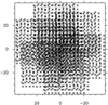 |
Fig. 1 Example of pointing positions for a single source in our OTF observations. The image is centred on the source and is in the units of arcsecond. |
2.3 Moment maps
We produced zeroth and first moment maps from the 13CO (6−5) data cubes, which show the distributions of the integrated intensity and velocity centroid on the sky. These maps are valuable tools for examining the morphology and kinematics of warm gas in the inner envelopes. For each pixel, zeroth and first moment values were calculated as follows:
 (1)
(1)
 (2)
(2)
where Ti and υi are the main-beam brightness temperature and velocity at each channel, respectively. To determine the velocity range for the integration of M0 and M1, an average spectrum was estimated from the whole data cube for each source using CLASS (individual spectra were weighted by observing times), and the range of velocity channels over which emission is clearly detected above 3σ (σ is the spectral noise) was determined based on visual inspection. During the integration for M0 and M1, velocity channels below 3σ were not included. Similarly, pixels whose peak-to-noise ratios are lower than three were considered as non-detections and were masked in our final maps.
3 Results
3.1 Detection statistics
In this section, we analyse the detection of 13CO (6−5) emission in our sources. For our analysis, we derived an average spectrum over the central region with a size of 20″ (close to one ATLAS- GAL beam and noise level is improved (Fig. 1)) for each source and considered a line to be detected if the peak main-beam brightness temperature was higher than 3σ.
We found that 13CO (6−5) emission is detected towards 81 clumps with varying detection rates among the evolutionary groups (Fig. 2). Specifically, the detection rate increases from 31%4 for the youngest group (70w) to 70–100% for more evolved groups (IRw, IRb, and HII) and is 83% for the whole sample. Similarly, the peak main-beam brightness temperature tends to increase towards the evolved source groups (Fig. 3). This increase in the detection rate and peak main-beam brightness temperature could indicate increasing density and/or temperature along the evolutionary sequence of high-mass star formation, considering that the enhancement in density and/or temperature is conducive to more easily exciting 13CO molecules to mid-J rotational levels. At the same time, the warmer environment could allow more frozen 13CO on dust grains to sublimate, enhancing the abundance of 13CO molecules in the gas and the chance to detect mid-J 13CO emission. Indeed, Giannetti et al. (2017) noted a difference between the IRw and IRb groups, finding CO to be mainly locked on dust grains in the former stage, while in the latter it exists mostly in the gas phase.
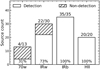 |
Fig. 2 Detection statistics of 13CO (6−5) emission for the evolutionary groups. The exact number of the detected sources for the observed clumps is presented at the top of each bar, and the corresponding detection rates are shown in percentage terms. |
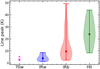 |
Fig. 3 Distributions of the peak brightness temperatures. These temperatures were obtained from the average spectra within the 20″ -size central regions. For each evolutionary group, the minimum and maximum are shown as bars, while the median values are indicated as filled circles. For the 70w group that has only a few entries, the values for the individual sources are presented as crosses. |
3.2 Line profiles
In this section, we examine the general shape of 13CO (6−5) line profiles based on the representative spectra of the different evolutionary groups. To produce these representative spectra, we shifted the average spectra of the central 20″ regions to 0 km s−1 according to C17O (3−2)-based source velocities (Giannetti et al. 2014) and calculated the average of all sources in each evolutionary group. Four clumps without C17O (3−2) data (two IRw, one IRb, and one HII) and one 70w source whose 12CO (6−5) spectra heavily affected by a contaminated reference position were excluded from our calculation. For comparison, we also produced representative 12CO (6−5) spectra in the same manner by using APEX 12CO (6−5) observations from Navarete et al. (2019).
Figure 4 shows that the 13CO (6−5) and 12CO (6−5) spectra have systematically different shapes. In general, the 13CO (6−5) spectra are much narrower and are not severely affected by selfabsorption, indicating that 13CO (6−5) and 12CO (6−5) emission likely traces different regions of (or different conditions within) the envelopes. For 81 sources with 13CO (6−5) detection in our sample, Navarete et al. (2019) indeed estimated that only 15 sources are not affected by self-absorption in their 12CO (6−5) spectra. We fitted a single Gaussian function to each of the13 CO (6−5) representative spectra (Fig. 4) to quantify the line width and found full width at half maximum (FWHM) values of 2.4, 4.4, 5.8, and 8.3 km s−1 for the 70w, IRw, IRb, and HII spectra, respectively. The increase in the FWHM is less likely to be affected by the opacity broadening effect as 13CO (6−5) emission is mostly optically thin (Appendix B). Instead, it is closely linked to the increase in the source size (Sect. 4.1; Larson’s size–line width relation) and suggests that non-thermal motions become stronger in evolved sources.
While a single Gaussian represents the overall shape of the 13CO (6−5) spectra reasonably well, residuals are visible at velocities of ∼5–10 km s−1 for the IRw, IRb, and HII groups, hinting at the existence of a secondary component. In the case of low-mass YSOs, 13CO (6−5) emission is considered to trace quiescent envelopes with an additional contribution from outflow cavity walls that are heated by UV photons, and/or from bow shocks or accretion discs (e.g. Spaans et al. 1995; van Kempen et al. 2009a,b). Our finding is consistent with the low-mass YSO results in that it indicates a complex origin of13 CO (6−5) emission; we will further discuss possible heating mechanisms for 13CO (6−5) emission in Sect. 5.1.
3.3 Line luminosities
To investigate further how the properties of 13CO (6−5) emission change with the evolution of high-mass star formation, we computed the line luminosity, LCO, and examined correlations between LCO and some of the key clump characteristics such as Lbol and Mclump. The line luminosity was calculated from the average spectra of the central 20″ regions based on the following equation:
 (3)
(3)
where D is the distance to each source and Fλ is the integrated intensity in Wm−2. The conversion from K km s−1 to W m−2 for Fλ was done following Eq. (2) in Indriolo et al. (2017):
 (4)
(4)
where v is the line frequency and Ω = πθ2/4ln(2) is the solid angle occupied by a Gaussian beam with a size θ = 20″. For the sources with detections, M0 values were calculated over the same velocity ranges used in Sect. 2.3. On the other hand, for the sources without detections, upper limits on LCO were estimated based on the 3σ values and the median velocity range for the sources with detections (27 km s−1).
Figure 5 presents the cumulative distributions of LCO for the detected sources. From these distributions, we found that the median LCO increases from the youngest to the most evolved group: 2.3 × 1024 W, 1.2 × 1025 W, 2.1 × 1025 W, and 9.3 × 1025 W for the 70w, IRw, IRb, and HII group, respectively. When k-sample Anderson-Darling tests were performed on each pair of the groups with sufficient numbers of sources (i.e. IRw, IRb, and HII) with a significance level of 0.05, all combinations except for the IRw-IRb pair were found to be drawn from different populations. These results suggest that the 13CO (6−5) luminosities are closely related to the evolutionary state of a source. As such, LCO is also correlated with two of the other evolutionary sequence indicators, Lbol and Mclump (König et al. 2017) (Fig. 6) with Spearman’s rank correlation coefficients of 0.93 and 0.86, respectively.
In addition, we found that our 13CO (6−5) luminosities are strongly correlated with the 12CO (6−5) luminosities from Navarete et al. (2019) (Fig. 7; Spearman’s rank correlation coefficient of 0.90). The correlation spans several orders of magnitude and remain continuous out to the high luminosity regime, which is surprising as one may expect it to flatten once the 12CO (6−5) emission becomes saturated due to its high opacity5 while the 13CO (6−5) emission is still optically thin (Appendix B). One plausible explanation for the continuous increase in the 12CO (6−5) luminosity could be a non-trivial contribution of optically thin high-velocity emission arising from outflows to the total emission. If this were the case, the strong correlation between the 13CO (6−5) and 12CO (6−5) luminosities would suggest that similar mechanisms would partly power the emission in both transitions (Sect. 5.1).
In summary, we found that 13CO (6−5) emission is ubiquitous in massive clumps, including in the youngest sources that do not yet harbour protostars. The increases in the detection rate, peak brightness temperature, and line width determined for evolved sources indicate systematic changes in physical conditions, such as density, temperature, CO column density, and non-thermal motions, along the sequence of high-mass star formation. Furthermore, the tight correlation of the 13CO (6−5) luminosity with the 12CO (6−5) luminosity, bolometric luminosity, and clump mass implies that the origin of 13CO (6−5) emission is likely linked to star formation processes.
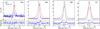 |
Fig. 4 Representative 12CO (6−5) (black) and 13CO (6−5) (blue) spectra of the four evolutionary groups. The 13CO (6−5) spectra are scaled up by a factor of two for an easier comparison, and the fitted Gaussian functions are overlaid as red curves. In the bottom panels, the residuals from Gaussian fitting are shown with ±3σ noise levels (dashed lines). |
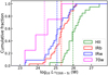 |
Fig. 5 Cumulative distributions of the 13CO (6−5) line luminosities. These luminosities were derived from the spectra averaged over the central 20″ regions. The median values of the four evolutionary groups are shown as dashed lines in different colours. |
3.4 Classification of our sources
Before probing the distribution and kinematics of warm molecular gas in detail (Sect. 4), we classified our sources based on their morphologies in the 13CO (6−5) integrated intensity maps. The block diagram for our classification is shown in Fig. 8, and examples of the such classified sources are presented in Fig. 9.
In essence, our classification is based on the extent and morphology of 13CO (6−5) emission. First, we considered sources with fewer than 16 detected pixels (corresponding to four telescope beams) as ‘poorly resolved’ and the rest as ‘well resolved’. An exception is G351.51+0.7, which is categorised as a poorly resolved clump in spite of its significant number of detected pixels as the pixels are scattered across the map. Among the well-resolved sources, we classified those with a single bright core in the map centre as ‘single-core’ or ‘extended’. Singlecore clumps have bright emission well confined in the map centre, while extended clumps show emission extending from the centre to the edge of the maps, implying that our maps capture only a part of larger structures. ATLASGAL 870 µm maps of these regions indeed reveal large complexes of dust condensations, whose structures are generally consistent with the observed 13CO (6−5) distributions (Appendix C). In addition to the simple single-core case described above, we also considered sources that have central cores along with additional peaks at the map outskirts as single-core, as the peripheral spots arise from neighbouring objects and can be masked out (Appendix D). Finally, we classified sources that have multiple central cores without extended emission as ‘fragmented-cores’.
Table 2 presents the number of sources in each category and evolutionary stage. In total, 59 sources are considered as well-resolved. The majority of them (52) are single-core sources, while the rest (7) show extended emission or signs of fragmentation. Interestingly, 50 out of the 59 well-resolved clumps (85%) have evolved to IRb and HII phases, while 17 out of the 22 poorly resolved clumps (77%) are in younger stages (70w and IRw). This result suggests that the four evolutionary groups are distinctive in terms of the spatial distribution of their 13CO (6−5) emission, as well as their peak brightness temperature.
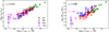 |
Fig. 6 13CO (6−5) line luminosity as a function of bolometric luminosity (left) and clump mass (right). The sources in the HII, IRb, IRw, and 70w groups are shown as green squares, red triangles, blue circles, and magenta diamonds, respectively. The Spearman’s rank correlation coefficient, rs, between the two quantities is presented on each plot. |
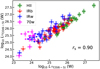 |
Fig. 7 Relation between the 13CO (6−5) and 12CO (6−5) line luminosities. The sources without 13CO (6−5) detections are indicated as leftward arrows whose locations represent 3σ values. The colours and markers are the same as in Fig. 6. |
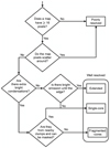 |
Fig. 8 Block diagram for our classification of sources based on our 13CO (6−5) integrated intensity maps. |
Number of sources in each category determined by the 13CO (6−5) integrated intensity maps.
4 Analyses
In this section, we investigate the distribution and kinematics of 13CO (6−5) emission in the envelopes of massive clumps by considering 52 single-core sources (Sect. 2.3). While the simplest morphology of these sources makes our analyses straightforward, we note that we are biased in favour of evolved envelopes as the majority of the single-core sources are in the IRb or HII group. As such, we do not put too much emphasis on the information on evolutionary trends derived here.
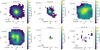 |
Fig. 9 Examples of the different morphological types in our sample. Top row: The first two panels show two single-core sources: the left one is an isolated source, while the right one has a neighbouring clump whose pixels outlined in red were masked to exclude them from further analyses. The most-right panel presents an extended source. Second row: The first panel showcases fragmented cores. The two remaining panels illustrate two poorly resolved clumps characterised by compact emission in neighbouring pixels (left) and distributed pixels (right). The hatched circle at the bottom left corner of each panel indicates the FWHM of telescope beam. |
4.1 Size and aspect ratio
We started our analyses by measuring the size of each source based on the total number of detected pixels. Specifically, we calculated the effective size, Seff, as the square root of the total emitting area and considered it as a representative size. The resultant cumulative distribution functions (Fig. 10) suggest that the 13CO emission regions associated with HII sources are generally larger than those found for IRw and IRb sources. For example, the median sizes of the three groups (IRw, IRb, and HII) are 0.59, 0.63, and 0.99 pc, respectively, while the S eff of the only 70w source is 0.37 pc. When a k-sample Anderson-Darling test was performed on the IRb and HII groups for which we have sufficient numbers of sources, the sizes of the HII envelopes were indeed found to be systematically larger at a significance level of 0.05.
In addition, we estimated the aspect ratio (APR) of each source by fitting a two-dimensional Gaussian function to the detected pixels in the integrated intensity image and found a range of 1.0–2.6 with a median of 1.3 and a standard deviation of 0.4. Considering that APRs vary with inclination angles and the members of our statistically significant sample of singlecore sources likely have a wide range of inclination angles, the measured small range of the APR implies that the envelopes are less likely to be filamentary structures whose minimum APR is defined as three (Mattern et al. 2018).
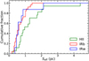 |
Fig. 10 Cumulative distribution functions of the effective size. The 70w group is not presented here, since it comprises only a single source. |
4.2 Radial intensity profiles
Next, we examined the spatial distribution of 13CO (6–5) emission by constructing the radial intensity profiles of our singlecore sources. To do so, we divided each M0 map into 5″-wide individual annuli centred on the peak location of 13CO (6–5) emission and calculated median and standard deviation values. Example radial profiles are presented in Fig. 11.
The constructed radial profiles were analysed with power-law functions following Beuther et al. (2002):
 (5)
(5)
where F(r) is the integrated intensity at a given radius r, m is the power-law index, and rb is the break radius within which the integrated intensity becomes constant (introduced to prevent F(r) from going to infinity as r approaches zero). This power-law function was devised based on the theoretical expectations for the structures of collapsing cores (e.g. Shu et al. 1987; McLaughlin & Pudritz 1996; Motte & André 2001) and was convolved with a 10″ -size Gaussian beam (comparable to our13 CO (6–5) angular resolution) to be fitted to our radial profiles.
To constrain the power-law index and break radius, we performed non-linear least squares fitting using the Python function scipy.optimize.curve_fit on the model and observed radial profiles. We excluded data points at large radii for which the number of detected pixels is less than 5% of the total pixels (e.g. open blue circles in Fig. 11) from fitting, as they are less likely to be statistically representative. The best-fit curves were found to reproduce the observed radial profiles reasonably well within 1σ uncertainties (hence obviating the need for a second power-law function), and their parameters are presented in Appendix A.
We examined the constrained power-law indices and break radii in detail by focusing on 36 sources (one 70w, four IRw, 17 IRb, and 14 HII sources) whose the best-fit parameters are statistically significant (i.e. higher than their 1σ uncertainties). The distributions of the power-law index for these sources are presented in Fig. 12. We find that the power-law index ranges from 0.5 to 2.7 across the entire sample and varies by less than a factor of three within each group, indicating relatively comparable slopes between the sources in the same evolutionary stage. Interestingly, there is a slight tendency for the power-law index to increase towards more evolved sources: median m values are 0.8, 1.1, and 1.5 for the IRw, IRb, and HII group, respectively. A k-sample Anderson-Darling test on the IRb and HII groups indeed suggests that the HII sources have distinctly steeper slopes than the IRb sources. These steeper slopes could result from a significant increase in the brightness of 13CO (6–5) emission in the central parts of the most evolved sources (e.g. Fig. 3), which is in turn most likely due to the strong enhancement in density and/or temperature.
In addition, we probed the constrained break radii and found that rb changes from 0.02 pc to 0.44 pc across the entire sample (Fig. 13). The variations in rb (e.g. a factor of 22 for the whole sample and a factor of 13 for the IRb sources) are much more significant than those in m, which partly reflects the sources’ wide range of distances. As in the case of m, rb tends to increase towards the most evolved sources (e.g. median rb of 0.05, 0.05, and 0.14 pc for the IRw, IRb, and HII group, respectively), and a k-sample Anderson-Darling test on the IRb and HII groups confirms this tendency.
While the break radius was introduced for a mathematical reason, it could manifest underlying physical conditions in the central parts of our sources, such as fragmentation on small scales and high opacity of the 13CO (6–5) emission. As for the fragmentation scenario, interferometric observations of massive star-forming clumps, including several of our sources, have indeed identified fragmented cores with sizes smaller than or comparable to our spatial resolution (≲0.1 pc) (Cesaroni et al. 2017; Beltrán et al. 2021). The convolution of these fragmented cores with our single-dish beam would smooth out small-scale structures and result in the uniform distribution of 13CO (6–5) emission in the source centres. Interestingly, Beuther et al. (2002) argued that more massive clumps tend to produce larger fragmented cores or clusters, which implies larger rb for more massive clumps. We indeed found such a positive correlation between rb and Mclump (Fig. 13, bottom), supporting the fragmentation scenario for the break radius. However, we also note that Mclump is related to D as Mclump ∝ D2 (König et al. 2017), which could partially contribute to the correlation between rb and Mclump.
Another possible explanation for the break radius is high opacity of 13CO (6–5) emission. When the 13CO (6–5) emission is optically thick, its brightness temperature approaches the gas kinetic temperature, resulting in the saturation of the integrated intensity. Our preliminary analysis based on local thermodynamic equilibrium (LTE) suggests that most of our sources likely have optically thin 13CO (6–5) emission (Appendix B). Besides, only a weak correlation exists between τ13CO and rb (Spearman’s rank correlation coefficient of 0.32). These results imply that the break radius is less likely to be determined by the effect of opacity.
In conclusion, we found that the radial intensity profiles of single-core clumps can be reasonably well described as powerlaw functions, indicating relatively simple structures of the envelopes of massive star-forming regions. The observed radial profiles retain comparable slopes within the same evolutionary group, while the most evolved sources tend to have steeper slopes that are likely related to star formation processes (higher densities and/or temperatures). In addition, fragmentation could begin in the early stage of high-mass star formation (70w) and be responsible for the uniform intensity distribution in the central parts of our sources.
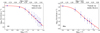 |
Fig. 11 Example 13CO (6–5) radial profiles for an HII source (G43.17+0.0) (left) and an IRw source (G335.79+0.1) (right). At 5″-wide individual annuli, the median and standard deviation values are presented as filled blue circles and associated ‘error’ bars. Annuli with an insufficient number of detected pixels are indicated as open blue circles and were excluded from the determination of best-fit curves (red). |
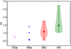 |
Fig. 12 Distributions of the power-law index, m, for the different evolutionary groups: 70w, IRw, IRb, and HII in magenta, blue, red, and green, respectively. The colours and symbol schemes are the same as in Fig. 3. |
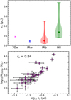 |
Fig. 13 Top: Distributions of the break radius, rb, for the different evolutionary groups. The colours and symbol schemes are the same as in Fig. 3. Bottom: Scatter plot between the clump mass and the break radius. The Spearman’s rank correlation coefficient is presented on the top left corner of the plot. |
4.3 Comparison between dust and warm molecular gas distributions
In this section, we examine how the distribution of warm molecular gas in high-mass star-forming regions compares to that of the colder medium by comparing 13CO (6–5) and 160 µm radial intensity profiles. For our examination, we employed Hi- GAL 160 µm maps as their angular resolution (11″ × 13″) is comparable to that of the 13CO (6–5) data (Molinari et al. 2010).
To derive radial profiles, Hi-GAL 160 µm maps with a size of 5′ × 5′ were first converted to the equatorial coordinate system to match the 13CO (6–5) data. Once the pixels with emission from nearby objects were masked (Appendix D), 160 µm radial profiles were constructed in the same manner as the 13CO (6–5) radial profiles (Sect. 4.2) and were cut off at 100″ to meet the angular extent of the 13CO (6–5) radial profiles. In total, we produced the 160 µm radial profiles for a sample of 36 sources for which we found reliable fitting parameters for the 13CO (6–5) radial profiles (Sect. 4.2).
Visual inspections of the derived radial profiles indicated the need for more than one power law for some sources (e.g. Fig. 14, right), prompting us to fit both single (Eq. (5)) and two powerlaw functions to the radial profiles. The two power-law model can be written as follows:
 (6)
(6)
where mi and mo are the indices for the inner and outer powerlaw functions,  is the break radius within which the central intensity distribution becomes constant, and
  is the transition radius from the inner to the outer power-law function. Both the single and two power-law models were convolved with a 12″- size Gaussian beam (average of the major and minor axes of the 160 µm beam) to be fitted to our radial profiles.
We performed the same non-linear least squares fitting as in Sect. 4.2 and found that the two power-law model significantly improves fitting results for 27 sources by lowering the reduced χ2 by more than a factor of two compared to the single powerlaw model. The radial profiles of the remaining nine sources were better described with the single power-law model, considering that the reduced χ2 was improved by less than a factor of two or the width of the inner power-law distribution was smaller than the 160 µm beam; in other words, the inner power-law distribution is not well constrained. The fitting results for all 36 sources were deemed reliable (i.e. fitting parameters above their 1σ uncertainties) and are summarised in Appendix A.
For 26 out of the 27 sources for which the two powerlaw model is favoured, we found mi > mo, which suggests that central compact cores are surrounded by extended diffuse structures. Interestingly, Beuther et al. (2002) found the opposite result (shallower inner gradients) from their analysis of 1.2 mm dust continuum emission in a number of massive star-forming regions. It is difficult to make a one-to-one comparison with our result, however, since the sources in Beuther et al. (2002) suffer from distance ambiguities and we cannot make sure if the 1.2 mm and 160 µm profiles probe comparable spatial extents.
The inner power-law distributions of the 160 µm radial profiles have on average similar extents as the 13CO (6–5) radial profiles (~40″), indicating that they probe comparable physical scales. Considering this, we directly compared the properties of the inner power-law distributions of the 160 µm radial profiles (power-law index and break radius) to those of the 13CO (6–5) radial profiles. To increase the sample size, we also considered the nine sources whose 160 µm radial profiles were fitted with the single power-law function. Figure 15 shows a positive correlation between the power-law indices of the 160 µm and 13CO (6–5) radial profiles. On closer inspection, the 160 µm profiles generally have steeper slopes, implying that 160 µm and 13CO (6–5) emission could trace different physical conditions or processes (e.g. 160 µm emission likely traces colder structures than 13CO (6–5) emission). Alternatively, the discrepancy in the power-law indices could result from the different dependencies of the two tracers on the gas temperature and density. Interestingly, the 160 µm radial profiles tend to be steeper towards more evolved sources, which is in line with what we found from the 13CO (6–5) radial profiles (Sect. 4.2). On the other hand, the break radii of the 160 µm and 13CO (6–5) radial profiles seem to be consistent in most cases, suggesting that the same mechanism (i.e. fragmentation) is likely responsible for the uniform distribution of 160 µm and 13CO (6–5) emission in the central parts of our sources.
In conclusion, we found that the 160 µm emission from our sources typically shows two distinct structures: compact cores and their surrounding diffuse halos. Compared to 160 µm emission, 13CO (6–5) emission from warm gas is more compact and probes mostly the core structures with its radial distribution decreasing less steeply. The emission from both tracers shows uniform intensity distributions in the centre of our sources, which likely originates from fragmentation on small scales.
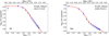 |
Fig. 14 Example 160 μm radial profiles of G43.17+0.0 (left) and G335.79+0.1 (right). As in Fig. 11, the median and standard deviation values at 5″ -wide individual annuli are shown as blue circles and associated ‘error’ bars. Best-fit curves (singular and two power-law model for G43.17+0.0 and G335.79+0.1, respectively) are overlaid in red. |
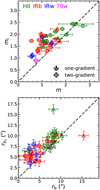 |
Fig. 15 Comparison of the 160 µm and 13CO (6–5) radial profiles in terms of the power-law index (top) and break radius (bottom). The 27 sources whose 160 µm radial profiles were fitted with the two powerlaw model are shown as circles, and their inner power-law distributions are used for the comparison. The remaining nine sources with the single power-law distributions in 160 µm emission are indicated as triangles. Both circles and triangles are colour coded based on evolutionary stage: 70w, IRw, IRb, and HII in magenta, blue, red, and green, respectively. One-to-one relations are overlaid as dashed lines. |
4.4 Mean velocity gradients
In addition to the spatial distribution, we examined the kinematics of warm molecular gas for the sources of our sample of high-mass star-forming regions by analysing the 13CO (6–5) first moment maps of our 52 single-core sources. Visual inspections of the 13CO (6–5) M1 maps reveal a variety of velocity fields, including linear gradients or more complex trends such as radial, hourglass-like, and outflow-like gradients (Fig. 16). Among these various velocity fields, the linear gradients are the most common (44 sources), while the other types occur much less often (eight sources).
To quantify the observed 13CO (6–5) velocity fields, we estimated the mean velocity gradients (MVGs) by fitting the following equation from Goodman et al. (1993) to our M1 maps using the Python function scipy.optimize.curve_fit:
 (7)
(7)
where υLSR is the velocity at a given pixel, υ0 is the velocity at a reference position, ∆α and ∆β are the right ascension (RA) and declination (Dec) offsets from the reference position measured in radians, and a and b are the projections of the velocity gradient per radian onto the RA and Dec axes. For this fitting, we fixed the reference position at the centre of each source, since the MVGs measure the general direction of gas motions and hence the fitted a and b do not depend on the reference position.
Once a and b were constrained, the magnitude of the MVG, 𝒢 (km s−1 pc−1), was computed as follows:
 (8)
(8)
where D is the distance to the source. In addition, the position angle (PA) of the MVG, θ𝒢 (degree), was measured counterclockwise from the north to the red-shifted gradient (i.e. red arrows in Fig. 18). Specifically, θ𝒢 was calculated from α = |tan−1 (a/b )| as follows:
 (9)
(9)
We examined the constrained 𝒢 for 41 sources (one 70w, 5 IRw, 21 IRb, and 14 HII sources) that have statistically significant gradients 𝒢 ≥ 3σ𝒢 (Goodman et al. 1993) and found that 𝒢 generally ranges from 1 km s−1 pc−1 to 8 km s−1 pc−1 independent of the evolutionary group (Fig. 17). An outlier is G351.77−0.5, whose large gradient of 20 km s−1 pc−1 likely originates from the strong outflow of the source. Interestingly, our median 𝒢 (~3 km s−1 pc−1) is comparable to that estimated by Tobin et al. (2011) for a sample of low-mass protostar envelopes (2 km s−1 pc−1). A one-to-one comparison of these results, however, is not straightforward, considering that the angular resolution of the study by Tobin et al. (2011) is three times larger than that of our data. On the other hand, the sources in that study are, at distances of 125–460 pc, much closer than the sources in our sample. As we demonstrate in Appendix E, the measurement of the MVGs depends on the physical resolution.
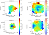 |
Fig. 16 Examples of various velocity fields in our sample. The 13CO (6–5) M1 maps from the top left corner in the clockwise direction demonstrate linear, radial, hourglass-like, and outflow-like gradients, respectively. For each source, the integrated intensities are overlaid as contours with levels ranging from 20% to 80% of the peak value in steps of 20%, and the peak position is marked by a star. Finally, the FWHM of the telescope beam is shown by a hatched circle. |
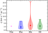 |
Fig. 17 Distributions of the MVG magnitude, 𝒢, for the different evolutionary groups. The colours and symbol schemes are the same as in Fig. 3. |
Possible interpretations of the observed gas kinematics.
4.5 Comparison of gas kinematics on different spatial scales
Section 4.4 shows that 13CO (6–5) emission in our single-core sources frequently shows linear velocity gradients. To provide insights into the origin of these velocity gradients, we compared gas kinematics on three different spatial scales, including outflows from small-scale YSO cores that are traced by high velocity 12CO (6–5) emission, intermediate-scale envelopes traced by 13CO (6–5) emission, and large-scale clumps traced by 13CO (2–1) emission. For sources in the early stage of star formation, we can expect that the intermediate-scale envelopes retain the kinematics of their parental clumps, inducing an alignment between the envelope and clump kinematics (e.g. Smith et al. 2011). As star formation progresses, strong outflows may be launched and entrain dense gas from the envelopes, resulting in an alignment between the outflow and envelope kinematics, similar to envelopes of Class 0 low-mass protostars (Arce & Sargent 2006). Once the outflows significantly erode into the envelopes, the remaining envelope material could be concentrated near the protostellar discs and be rotating together, leading to a perpendicular alignment between the outflow and envelope kinematics, similar to what is found in envelopes of low-mass Class I protostars by Arce & Sargent (2006). These possible scenarios demonstrate that the comparison of gas kinematics on different spatial scales can be valuable for understanding the processes of high-mass star formation.
We started our comparison of gas kinematics by evaluating how velocity fields of the outflows and the envelopes are linked to each other. To do so, we utilised 12CO (6–5) outflow data from Navarete et al. (in preparation) and examined the absolute angular difference ∆PA1 = | PA of the 13CO (6–5) MVGs – PA of the 12CO (6–5) outflows | (Fig. 18 and Appendix F). Navarete et al. identified outflow sources in the Top100 sample by integrating 12CO (6–5) emission in high-velocity wings and divided them into several categories, such as single, multiple, unresolved, and resolved (defined as clearly separated blue and red lobes) outflows. For our examination, we computed ∆PA1 for 22 sources (one 70w, three IRw, twelve IRb, and six HII sources) that have single resolved outflows along with significant 13CO (6–5) MVGs and compared the resultant distributions for the different evolutionary groups. Figure 19 shows that the ∆PA1 distributions support neither the envelope entrainment (∆PA1 ~ 0°) nor the envelope-disc co-rotation (∆PA1 ~ 90°) and are not significantly different between the evolutionary groups.
In addition, we probed a relation between the envelope and clump kinematics by comparing the 13CO (6–5) and 13CO (2–1) MVGs. To derive 13CO (2–1) MVGs for our single-core sources, we used data from the SEDIGISM survey (Schuller et al. 2021) and produced 2′ × 2′ sized M0 and M1 maps (Fig. 20). The 2′ × 2′ maps, which are ~1.5 times larger than our 13CO(6-5) maps, were chosen as they include a majority of the regions in which the 13CO (2–1) line’s intensity is higher than 40% of the peak value. With the resultant M0 and M1 maps, we then estimated MVGs by applying Eqs. (8) and (9) and found that 23 sources (two IRw, twelve IRb, and nine HII sources) have statistically significant MVGs in both 13CO (2–1) and 13CO (6–5) emission. The estimated 13CO (2–1) MVGs are presented in Appendix A.
In Fig. 21, we compared the magnitudes of the 13CO (6–5) and 13CO(2–1) MVGs and found that 𝒢 is generally higher in 13CO (6–5) emission. For example, the median magnitudes of the 13CO(6–5) and 13CO(2–1) MVGs are 2.8 km s−1 pc−1 and 0.7 km s−1 pc−1, respectively. The smaller 𝒢 for 13CO (2–1) could partially result from the coarser angular resolution of the SEDIGISM data compared to our 13CO (6–5) beam (30″ versus 10″; see Appendix E for further discussion). In addition, we examined the absolute angular difference ∆PA2 = | PA of the 13CO (6–5) MVGs – PA of the 13CO (2–1) MVGs | (Fig. 22) and found that 13 sources have relatively comparable PAs in both transitions (∆PA2 ≲ 45°), while the remaining 10 sources show a wide range of the angular difference. Interestingly, both the magnitude and PA comparisons show no dependence on the evolutionary groups.
Finally, we examined the relationship between the outflow, envelope, and clump kinematics more comprehensively by comparing the 12CO (6–5), 13CO (6–5), and 13CO (2–1) velocity information for a smaller sample of 15 sources. For our comparison, we considered six possibilities based on the measured ∆PA1 and ∆PA2 (Table 3) and examined them along with the M1 maps. This detailed view on the individual sources revealed that the origin of the13 CO (6–5) kinematics is relatively clear for seven sources only. For example, the 13CO (6–5) kinematics is likely decoupled from the surrounding clumps for four sources. Three of them (G330.95−0.1, G332.09−0.3, and G337.92−0.4; two IRb and one HII sources) show a hint of the envelope entrainment, while G305.21+0.2 (IRb) has co-rotating envelope and disc. In addition, two sources (G335.79+0.1 and G345.00−0.2; that is, one IRw and one HII source) show coherent rotations of the envelopes and clumps along the outflow axes. The 13CO (6–5) kinematics of the remaining source G337.41−0.4 (HII) seems to be dominated by the surrounding clump with no obvious impact from outflows.
In summary, we found that our single-core sources have significant linear velocity gradients in 13CO (6–5) emission. The origin of these velocity gradients is currently unclear, although it is less likely to be systematically linked to internal star formation processes (that is, 𝒢 does not vary much between the different evolutionary groups). The envelope kinematics traced by 13CO (6−5) emission appears to be highly complex, and probing its origin would benefit from higher sensitivity, higher resolution observations of a bigger sample of high-mass star-forming regions.
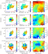 |
Fig. 18 Comparison of 13CO (6−5), 12CO (6−5), and 13CO (2−1) gas kinematics for four example sources. Left column: M1 maps of 13CO (6−5) emission. For each source, the blue and red lobes of 12CO (6−5) outflows are overlaid as contours with decreasing levels ranging from 95% of the peak integrated intensities down to the first level above 3σ, in steps of 20% peak values. For G309.38−0.1 and G343.76−0.1 (Appendix F), a threshold of 2σ was used instead. The velocity ranges over which the blue and red lobes were integrated are presented at the bottom left, while the absolute angular difference between the PAs of the13 CO (6−5) and 12CO (6−5) MVGs (Δ PA1) is shown at the top left. Middle column: Same M1 maps as in the left panel, but with the 13CO (6−5) integrated intensities as contours (20% to 80% of the peak values in steps of 20%). The centre of each source with the maximum integrated intensity is indicated as a black star, while the direction of the 13CO (6−5) MVG is shown as blue and red arrows. The absolute angular difference between the PAs of the13 CO (6−5) and 13CO (2−1) MVGs (Δ PA2) is summarised at the bottom left. Right column: M1 maps of13 CO (2−1) emission. The13 CO (2−1) integrated intensities are shown as contours with levels ranging from 40% to 90% of the peak values in steps of 10%, while the directions of the 13CO (2−1) MVGs are indicated as blue and red arrows. The centres of the sources with the peak integrated intensities are marked as white stars. Finally, for each plot, the FWHM of corresponding telescope beam is displayed by a hatched circle. |
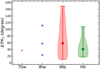 |
Fig. 19 Distributions of the absolute angular difference ΔPA1 for the different evolutionary groups. The colours and symbol schemes are the same as in Fig. 3. |
5 Discussion
Our observations of 13CO(6−5) emission towards a statistically significant sample of massive star-forming regions have allowed us to characterise the warm envelopes surrounding high-mass YSOs. In this section, we discuss potential origins of the emission and examine 13CO (6−5) kinematics in detail for several of our sources.
5.1 Excitation of13 CO (6−5) emission in massive star-forming regions
Key characteristics of the Top100 sources, such as gas temperature and column density, have been examined by various authors based on multi-transition observations of molecular species. For example, Giannetti et al. (2017) derived temperature by analysing emission from CH3CN, CH3 CCH, and CH3OH and found a progressive warm-up of the molecular gas with evolution that likely results from stellar feedback. In addition, Giannetti et al. (2014) showed that the abundance of CO molecules in the gas phase increases with evolution, as warmer dust grains enable frozen CO molecules to sublimate efficiently. A combination of the increased temperature and CO column density in the Top100 sources would excite more CO molecules to mid-J levels, resulting in the observed increase in the 13CO(6−5) brightness temperature (Sect. 3.1) and line luminosity (Sect. 3.3). This suggests that 13CO (6−5) emission can be used efficiently to probe the processes of high-mass star formation.
The warm molecular gas traced by mid-J 13CO emission can be heated by a range of radiative and mechanical feedback processes. For nearby low-mass star-forming regions, these processes can be probed in detail and observational and theoretical studies have suggested that mid-J13 CO emission originates from passively heated envelopes, UV-heated outflow cavity walls, and outflows themselves (van Kempen et al. 2009a,b; Yıldız et al. 2012). Considering that envelopes and outflows are also prevalent in regions of high-mass star formation, the observed 13CO (6−5) emission in the Top100 sources could have similar origins.
In the scenario of passively heated envelopes, dust grains are warmed up by absorbing radiation from central protostars and subsequently heat up the surrounding molecular gas via gas-dust collisions (Jørgensen et al. 2002; Kristensen et al. 2012). This mechanism has been shown to be responsible for part of the observed 13CO (6−5) emission in a large sample of low-mass YSOs (Yıldız et al. 2015). While the same mechanism could certainly work for high-mass star-forming regions, dedicated modelling of gas and dust in massive envelopes is required to assess the exact role of passive heating on the excitation of13 CO (6−5) emission in such complex systems.
In addition to the passively heated envelopes, 13CO (6−5) emission could partly arise from UV-heated outflow cavity walls. For low-mass YSOs, UV photons can be created from disc-protostar accretion boundary layers or shocked spots along outflows. These UV photons escape through outflow cavities and are scattered by dust grains on their way, producing PDRs along the cavity walls (Spaans et al. 1995; Yıldız et al. 2015). While the efficacy of the same mechanism for high-mass star-forming regions has not been confirmed, PDRs have been observed towards many massive YSOs, in particular evolved ones whose intense UV radiation can ionise hydrogen atoms in significant volumes around them. For example, Leurini et al. (2013) analysed a number of mid-J CO maps for G327.3−0.6 and found that the emission lines, including 13CO (6−5), are dominated by the PDR around a local HII region. In addition, multiple PDR layers have been proposed to reproduce the 13CO (6−5) observations of several high-mass star-forming regions, such as Cepheus A, DR21, and W49 (Graf et al. 1993; Koester et al. 1994). Interestingly, our HII sources have 13CO (6−5) brightness temperatures that are comparable to those measured by Graf et al. (1993), implying a non-negligible impact of UV photons on the excitation of 13CO (6−5) emission in our most evolved sources.
Finally, mechanical processes such as outflows could contribute to the excitation of 13CO (6−5) emission. For example, Yıldız et al. (2012) showed that 13CO (6−5) spectra towards the low-mass protostar NGC 1333 IRAS 4A and 4B have both narrow and broad components with FWHMs of ~2 km s–1 and ~10 km s–1. The same type of broad component has been found in low-J (Yang et al. 2018) and mid-J 13CO transitions (Sect. 3.2) for ATLASGAL sources, implying that outflows are capable of entraining and heating the 13CO-traced dense gas in massive star-forming regions. Currently, there is a lack of shock modelling effort to study the excitation of mid-J 13CO emission in outflows, and future studies are needed. In addition to outflows, other mechanical processes during high-mass star formation, such as accretion flows onto clumps and gravitational collapse of clumps (Heitsch et al. 2009; Vazquez-Semadeni et al. 2019), could also inject a significant amount of energy into the surrounding medium and excite 13CO (6−5) emission. This mechanism could be vital in particular for early-type clumps without central heating sources where gravitational collapse has just started (Pillai et al. 2023).
All in all, our study demonstrates that 13CO (6−5) emission is ubiquitous in a variety of massive clumps, ranging from young sources where protostars have not been yet formed to evolved sources with strong HII regions. This suggests that 13CO (6−5) emission could be excited by different processes at different epochs of high-mass star formation.
5.2 13CO (6−5) kinematics in individual clumps
Our velocity analyses for a statistically significant sample suggest the complex nature of 13CO (6−5) kinematics in high-mass star-forming regions (Sects. 4.4 and 4.5). In an attempt to shed more light on the processes that drive 13CO (6−5) kinematics, we present here a detailed examination of several individual sources based on complementary information from literature. Our source selection was based on the availability of kinematics information from other tracers, especially those with high spatial resolutions.
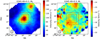 |
Fig. 20 13CO(2−1) M0 (left) and M1 (right) maps of an example source, G345.49+0.3. In both maps, the integrated intensities are overlaid as contours with levels ranging from 40% to 90% in steps of 10% of the largest integrated intensity. The 80″ × 80″ coverages of the 13CO (6−5) data are outlined as dashed red boxes, while the 2′ × 2′ regions where we extracted clump-scale kinematics are indicated by solid red boxes. At the left bottom corner of each map, the FWHM of the telescope beam is shown by a hatched circle. |
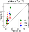 |
Fig. 21 Comparison between the magnitudes of the 13CO (6−5) and 13CO(2−1) MVGs (IRw, IRb, and HII group in blue, red, and green, respectively). A one-to-one relation is indicated by the dashed grey line. |
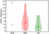 |
Fig. 22 Distributions of the absolute angular difference ΔPA2 for the different evolutionary groups. The colours and symbol schemes are the same as in Fig. 12. |
G43.17+0.0 (HII)
This HII region source is a part of the well-studied Galactic mini-starburst complex W49A, whose enhanced star formation efficiency has been attributed to various processes, including gravitational collapse (Welch et al. 1987), a cloud-cloud collision (Serabyn et al. 1993), expanding shells (Peng et al. 2010), and re-collapsing shells (Rugel et al. 2019). In our observations, 13CO(6−5) emission appears across a region of Seff ~ 4.4 pc, which is embedded within a surrounding structure that is at least 10 pc in diameter. The measured velocity centroids show a radial velocity gradient (Fig. 16) that could result from local collapse considering that the convergence of the gradient points towards the centre of our map. Another possibility is that 13CO (6−5) emission traces expanding shells. For example, the observed 13CO (6−5) spectra show double peaks in many places, whose velocities are consistent with those of the shells identified in C180(2−1) emission (Peng et al. 2010). However, in this case, it is not entirely clear how the expanding shells result in the radial velocity gradient.
G31.41+0.3 (HII)
This HII region source harbours a hot molecular core that has been extensively studied with multiple molecular species. For example, Cesaroni et al. (2017) performed CH3CN observations and found a rotating and infalling toroid on ~0.1 pc scales. In addition, Beltrán et al. (2022) identified at least six outflows with lobe sizes of ~0.02−0.2pc in SiO (5−4) observations. Compared to these small-scale observations, our 13CO (6−5) data probe a factor of ~10 larger region and show a linear gradient in velocity centroids (Fig. 23). Interestingly, the direction of the linear velocity gradient is perpendicular to that of the strongest SiO (5−4) outflow, implying a rotating 13CO (6−5) envelope. However, the rotation axis of the envelope is not aligned with that of the small-scale toroid, hampering us from pinpointing the exact origin of 13CO (6−5) kinematics.
G35.20−0.7 (IRb)
As a well-known star-forming region, G35.20−0.7 hosts an elongated dust structure that is embedded within a butterfly-shaped reflection nebula (Sánchez-Monge et al. 2013). Compared to the size of the observed 13CO (6−5) envelope, the elongated structure is roughly one third in length, while the reflection nebula is on a similar scale. Sánchez-Monge et al. (2014) argued that the elongated structure is a filament, rather than an edge-on rotating disc, based on C17O(3−2) and H13CO+ (4−3) observations and further suggested that G35.20−0.7 is a convergence centre of multiple filaments. Interestingly, the velocity range of 31–37 km s–1 along the elongated structure is comparable to the 13CO (6−5) velocity gradient, implying that 13CO (6−5) kinematics could trace the gas flow within the supposed converging filaments.
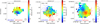 |
Fig. 23 13CO (6−5) M1 maps of G31.41+0.3, G35.20−0.7, and G351.77−0.5. The descriptions for the overlaid contours, symbols, and labels are the same as in Fig. 18. |
G351.77−0.5 (IRb)
The 13CO (6−5) first moment map of G351.77−0.5 clearly shows blue-shifted and red-shifted lobes (Fig. 23), suggesting an outflow origin of 13CO (6−5) kinematics. Other studies have identified outflows in this region as well. For example, Navarete et al. (in preparation) found an outflow traced by 12CO (6−5) emission (blue and red contours in Fig. 23), whose PA is slightly different from that of our 13CO (6−5) outflow. In addition, Leurini et al. (2009, 2011) detected three outflows in high-resolution (5.45″ × 2.08″) 12CO (2−1) observations. Among the three outflows, two are relatively well-aligned with the12 CO (6−5) outflow on a similar scale. The angular offset between the 13CO (6−5) and 12CO outflows suggests that different transitions and isotopologues of CO molecules probe different parts of the complex outflow system in G351.77−0.5.
In summary, our detailed examination of the four individual clumps supports the previous conclusion that 13CO(6−5) kinematics has a complex nature. Both small-scale (e.g. outflows) and large-scale (e.g. expanding shells and gas flows along filaments) processes impact on the kinematics of warm envelopes, and understanding their impact would be essential to elucidate how 13CO(6−5) emission is excited in massive star-forming regions.
6 Conclusions
In this paper, we characterised 13CO(6−5) emission towards ~100 massive star-forming clumps at different evolutionary stages. Our APEX observations with high angular and spectral resolutions allowed us to examine the morphology and kinematics of warm envelopes for a statistically significant sample. We summarise our main results and conclusions as follows:
The 13CO (6−5) emission line is detected towards sources at all stages of high-mass star formation. Key characteristics of the emission line, including the detection rate, line width, and peak brightness temperature, increase with evolutionary stages. In addition, the line luminosity is tightly correlated with the bolometric luminosity and the clump mass. These results suggest that the 13CO (6−5) emission line is related to star formation processes;
The 13CO(6−5) integrated intensity images show that a majority of the warm envelopes have a simple single-core morphology and the most evolved clumps (HII) have larger envelopes. The radial intensity profiles of the single-core clumps can be reasonably well described as single power-law functions. Interestingly, the slopes of the most evolved group (HII), tend to be steeper, possibly due to enhancements in density and/or temperature at the central parts of the warm envelopes;
The kinematics of the warm envelopes presents various forms and is likely not driven by a single physical process. While most of the single-core envelopes show significant linear velocity gradients, the origin of these gradients is unclear in many cases. A detailed examination of individual sources suggests that the gas motions in the warm envelopes could be driven by stellar feedback such as outflows and/or by inheriting the kinematics of large-scale parental clouds.
Data availability
Appendices of this paper are available on Zenodo at https://doi.org/10.5281/zenodo.14748231.
Acknowledgements
The authors thank the anonymous referee for the constructive report that helped us improve this paper. We thank MPIfR and APEX staff for operating the observatory and collecting the data. The work of FN is supported by NOIRLab, which is managed by the Association of Universities for Research in Astronomy (AURA) under a cooperative agreement with the National Science Foundation. Herschel was an ESA space observatory with science instruments provided by European-led Principal Investigator consortia and with important participation from NASA.
References
- Arce, H. G., & Sargent, A. I. 2006, ApJ, 646, 1070 [NASA ADS] [CrossRef] [Google Scholar]
- Beltrán, M. T., & de Wit, W. J. 2016, A&A Rev., 24, 6 [CrossRef] [Google Scholar]
- Beltrán, M. T., Rivilla, V. M., Cesaroni, R., et al. 2021, A&A, 648, A100 [Google Scholar]
- Beltrán, M. T., Rivilla, V. M., Cesaroni, R., et al. 2022, A&A, 659, A81 [NASA ADS] [CrossRef] [EDP Sciences] [Google Scholar]
- Beuther, H., Schilke, P., Menten, K. M., et al. 2002, ApJ, 566, 945 [Google Scholar]
- Bonnell, I. A., & Bate, M. R. 2006, MNRAS, 370, 488 [NASA ADS] [CrossRef] [Google Scholar]
- Bonnell, I. A., Bate, M. R., Clarke, C. J., & Pringle, J. E. 2001, MNRAS, 323, 785 [Google Scholar]
- Cesaroni, R., Sánchez-Monge, Á., Beltrán, M. T., et al. 2017, A&A, 602, A59 [NASA ADS] [CrossRef] [EDP Sciences] [Google Scholar]
- Csengeri, T., Leurini, S., Wyrowski, F., et al. 2016, A&A, 586, A149 [NASA ADS] [CrossRef] [EDP Sciences] [Google Scholar]
- Giannetti, A., Wyrowski, F., Brand, J., et al. 2014, A&A, 570, A65 [NASA ADS] [CrossRef] [EDP Sciences] [Google Scholar]
- Giannetti, A., Leurini, S., Wyrowski, F., et al. 2017, A&A, 603, A33 [NASA ADS] [CrossRef] [EDP Sciences] [Google Scholar]
- Goodman, A. A., Benson, P. J., Fuller, G. A., & Myers, P. C. 1993, ApJ, 406, 528 [Google Scholar]
- Graf, U. U., Eckart, A., Genzel, R., et al. 1993, ApJ, 405, 249 [NASA ADS] [CrossRef] [Google Scholar]
- Güsten, R., Nyman, L. Å., Schilke, P., et al. 2006, A&A, 454, L13 [NASA ADS] [CrossRef] [EDP Sciences] [Google Scholar]
- Güsten, R., Baryshev, A., Bell, A., et al. 2008, SPIE Conf. Ser., 7020, 702010 [Google Scholar]
- Heitsch, F., Ballesteros-Paredes, J., & Hartmann, L. 2009, ApJ, 704, 1735 [NASA ADS] [CrossRef] [Google Scholar]
- Hopkins, P. F., Kereš, D., Oñorbe, J., et al. 2014, MNRAS, 445, 581 [NASA ADS] [CrossRef] [Google Scholar]
- Indriolo, N., Bergin, E. A., Goicoechea, J. R., et al. 2017, ApJ, 836, 117 [Google Scholar]
- Jørgensen, J. K., Schöier, F. L., & van Dishoeck, E. F. 2002, A&A, 389, 908 [CrossRef] [EDP Sciences] [Google Scholar]
- Kasemann, C., Güsten, R., Heyminck, S., et al. 2006, SPIE Conf. Ser., 6275, 62750N [NASA ADS] [Google Scholar]
- Kauffmann, J., Pillai, T., Shetty, R., Myers, P. C., & Goodman, A. A. 2010, ApJ, 712, 1137 [NASA ADS] [CrossRef] [Google Scholar]
- Kennicutt, R. C. 2005, in Massive Star Birth: A Crossroads of Astrophysics, 227, eds. R. Cesaroni, M. Felli, E. Churchwell, & M. Walmsley, 3 [NASA ADS] [Google Scholar]
- Klapper, G., Lewen, F., Gendriesch, R., Belov, S. P., & Winnewisser, G. 2000, J. Mol. Spectrosc., 201, 124 [NASA ADS] [CrossRef] [Google Scholar]
- Koester, B., Stoerzer, H., Stutzki, J., & Sternberg, A. 1994, A&A, 284, 545 [NASA ADS] [Google Scholar]
- König, C., Urquhart, J. S., Csengeri, T., et al. 2017, A&A, 599, A139 [Google Scholar]
- Kristensen, L. E., van Dishoeck, E. F., Bergin, E. A., et al. 2012, A&A, 542, A8 [NASA ADS] [CrossRef] [EDP Sciences] [Google Scholar]
- Lee, M. Y., Wyrowski, F., Menten, K., Tiwari, M., & Güsten, R. 2022, A&A, 664, A80 [NASA ADS] [CrossRef] [EDP Sciences] [Google Scholar]
- Leurini, S., Codella, C., Zapata, L. A., et al. 2009, A&A, 507, 1443 [NASA ADS] [CrossRef] [EDP Sciences] [Google Scholar]
- Leurini, S., Codella, C., Zapata, L., et al. 2011, A&A, 530, A12 [NASA ADS] [CrossRef] [EDP Sciences] [Google Scholar]
- Leurini, S., Wyrowski, F., Herpin, F., et al. 2013, A&A, 550, A10 [NASA ADS] [CrossRef] [EDP Sciences] [Google Scholar]
- Mattern, M., Kauffmann, J., Csengeri, T., et al. 2018, A&A, 619, A166 [NASA ADS] [CrossRef] [EDP Sciences] [Google Scholar]
- Matteucci, F. 2021, A&A Rev., 29, 5 [NASA ADS] [CrossRef] [Google Scholar]
- McKee, C. F., & Tan, J. C. 2003, ApJ, 585, 850 [Google Scholar]
- McLaughlin, D. E., & Pudritz, R. E. 1996, ApJ, 469, 194 [Google Scholar]
- Molinari, S., Swinyard, B., Bally, J., et al. 2010, PASP, 122, 314 [Google Scholar]
- Motte, F., & André, P. 2001, A&A, 365, 440 [NASA ADS] [CrossRef] [EDP Sciences] [Google Scholar]
- Motte, F., Bontemps, S., & Louvet, F. 2018, ARA&A, 56, 41 [NASA ADS] [CrossRef] [Google Scholar]
- Müller, H. S. P., Thorwirth, S., Roth, D. A., & Winnewisser, G. 2001, A&A, 370, L49 [Google Scholar]
- Müller, H. S. P., Schlöder, F., Stutzki, J., & Winnewisser, G. 2005, J. Mol. Struct., 742, 215 [Google Scholar]
- Navarete, F., Leurini, S., Giannetti, A., et al. 2019, A&A, 622, A135 [NASA ADS] [CrossRef] [EDP Sciences] [Google Scholar]
- Padoan, P., Pan, L., Juvela, M., Haugbølle, T., & Nordlund, Å. 2020, ApJ, 900, 82 [NASA ADS] [CrossRef] [Google Scholar]
- Peng, T. C., Wyrowski, F., van der Tak, F. F. S., Menten, K. M., & Walmsley, C. M. 2010, A&A, 520, A84 [NASA ADS] [CrossRef] [EDP Sciences] [Google Scholar]
- Pillai, T. G. S., Urquhart, J. S., Leurini, S., et al. 2023, MNRAS, 522, 3357 [NASA ADS] [CrossRef] [Google Scholar]
- Rugel, M. R., Rahner, D., Beuther, H., et al. 2019, A&A, 622, A48 [NASA ADS] [CrossRef] [EDP Sciences] [Google Scholar]
- Sánchez-Monge, Á., Cesaroni, R., Beltrán, M. T., et al. 2013, A&A, 552, L10 [NASA ADS] [CrossRef] [EDP Sciences] [Google Scholar]
- Sánchez-Monge, Á., Beltrán, M. T., Cesaroni, R., et al. 2014, A&A, 569, A11 [NASA ADS] [CrossRef] [EDP Sciences] [Google Scholar]
- Schuller, F., Menten, K. M., Contreras, Y., et al. 2009, A&A, 504, 415 [NASA ADS] [CrossRef] [EDP Sciences] [Google Scholar]
- Schuller, F., Urquhart, J. S., Csengeri, T., et al. 2021, MNRAS, 500, 3064 [Google Scholar]
- Serabyn, E., Guesten, R., & Schulz, A. 1993, ApJ, 413, 571 [Google Scholar]
- Shu, F. H., Adams, F. C., & Lizano, S. 1987, ARA&A, 25, 23 [Google Scholar]
- Smith, R. J., Glover, S. C. O., Bonnell, I. A., Clark, P. C., & Klessen, R. S. 2011, MNRAS, 411, 1354 [NASA ADS] [CrossRef] [Google Scholar]
- Spaans, M., Hogerheijde, M. R., Mundy, L. G., & van Dishoeck, E. F. 1995, ApJ, 455, L167 [NASA ADS] [Google Scholar]
- Tobin, J. J., Hartmann, L., Chiang, H.-F., et al. 2011, ApJ, 740, 45 [NASA ADS] [CrossRef] [Google Scholar]
- Urquhart, J. S., Wells, M. R. A., Pillai, T., et al. 2022, MNRAS, 510, 3389 [NASA ADS] [CrossRef] [Google Scholar]
- van Kempen, T. A., van Dishoeck, E. F., Güsten, R., et al. 2009a, A&A, 507, 1425 [NASA ADS] [CrossRef] [EDP Sciences] [Google Scholar]
- van Kempen, T. A., van Dishoeck, E. F., Güsten, R., et al. 2009b, A&A, 501, 633 [NASA ADS] [CrossRef] [EDP Sciences] [Google Scholar]
- Vázquez-Semadeni, E., Palau, A., Ballesteros-Paredes, J., Gómez, G. C., & Zamora-Avilés, M. 2019, MNRAS, 490, 3061 [Google Scholar]
- Welch, W. J., Dreher, J. W., Jackson, J. M., Terebey, S., & Vogel, S. N. 1987, Science, 238, 1550 [Google Scholar]
- Wyrowski, F., Güsten, R., Menten, K. M., et al. 2016, A&A, 585, A149 [NASA ADS] [CrossRef] [EDP Sciences] [Google Scholar]
- Yang, A. Y., Thompson, M. A., Urquhart, J. S., & Tian, W. W. 2018, ApJS, 235, 3 [Google Scholar]
- Yildiz, U. A., Kristensen, L. E., van Dishoeck, E. F., et al. 2012, A&A, 542, A86 [NASA ADS] [CrossRef] [EDP Sciences] [Google Scholar]
- Yildiz, U. A., Kristensen, L. E., van Dishoeck, E. F., et al. 2015, A&A, 576, A109 [NASA ADS] [CrossRef] [EDP Sciences] [Google Scholar]
- Zinnecker, H., & Yorke, H. W. 2007, ARA&A, 45, 481 [Google Scholar]
The 12CO (6−5) profiles often suffer from self-absorption (Fig. 4).
All Tables
Number of sources in each category determined by the 13CO (6−5) integrated intensity maps.
All Figures
|
Fig. 1 Example of pointing positions for a single source in our OTF observations. The image is centred on the source and is in the units of arcsecond. |
| In the text | |
|
Fig. 2 Detection statistics of 13CO (6−5) emission for the evolutionary groups. The exact number of the detected sources for the observed clumps is presented at the top of each bar, and the corresponding detection rates are shown in percentage terms. |
| In the text | |
|
Fig. 3 Distributions of the peak brightness temperatures. These temperatures were obtained from the average spectra within the 20″ -size central regions. For each evolutionary group, the minimum and maximum are shown as bars, while the median values are indicated as filled circles. For the 70w group that has only a few entries, the values for the individual sources are presented as crosses. |
| In the text | |
|
Fig. 4 Representative 12CO (6−5) (black) and 13CO (6−5) (blue) spectra of the four evolutionary groups. The 13CO (6−5) spectra are scaled up by a factor of two for an easier comparison, and the fitted Gaussian functions are overlaid as red curves. In the bottom panels, the residuals from Gaussian fitting are shown with ±3σ noise levels (dashed lines). |
| In the text | |
|
Fig. 5 Cumulative distributions of the 13CO (6−5) line luminosities. These luminosities were derived from the spectra averaged over the central 20″ regions. The median values of the four evolutionary groups are shown as dashed lines in different colours. |
| In the text | |
|
Fig. 6 13CO (6−5) line luminosity as a function of bolometric luminosity (left) and clump mass (right). The sources in the HII, IRb, IRw, and 70w groups are shown as green squares, red triangles, blue circles, and magenta diamonds, respectively. The Spearman’s rank correlation coefficient, rs, between the two quantities is presented on each plot. |
| In the text | |
|
Fig. 7 Relation between the 13CO (6−5) and 12CO (6−5) line luminosities. The sources without 13CO (6−5) detections are indicated as leftward arrows whose locations represent 3σ values. The colours and markers are the same as in Fig. 6. |
| In the text | |
|
Fig. 8 Block diagram for our classification of sources based on our 13CO (6−5) integrated intensity maps. |
| In the text | |
|
Fig. 9 Examples of the different morphological types in our sample. Top row: The first two panels show two single-core sources: the left one is an isolated source, while the right one has a neighbouring clump whose pixels outlined in red were masked to exclude them from further analyses. The most-right panel presents an extended source. Second row: The first panel showcases fragmented cores. The two remaining panels illustrate two poorly resolved clumps characterised by compact emission in neighbouring pixels (left) and distributed pixels (right). The hatched circle at the bottom left corner of each panel indicates the FWHM of telescope beam. |
| In the text | |
|
Fig. 10 Cumulative distribution functions of the effective size. The 70w group is not presented here, since it comprises only a single source. |
| In the text | |
|
Fig. 11 Example 13CO (6–5) radial profiles for an HII source (G43.17+0.0) (left) and an IRw source (G335.79+0.1) (right). At 5″-wide individual annuli, the median and standard deviation values are presented as filled blue circles and associated ‘error’ bars. Annuli with an insufficient number of detected pixels are indicated as open blue circles and were excluded from the determination of best-fit curves (red). |
| In the text | |
|
Fig. 12 Distributions of the power-law index, m, for the different evolutionary groups: 70w, IRw, IRb, and HII in magenta, blue, red, and green, respectively. The colours and symbol schemes are the same as in Fig. 3. |
| In the text | |
|
Fig. 13 Top: Distributions of the break radius, rb, for the different evolutionary groups. The colours and symbol schemes are the same as in Fig. 3. Bottom: Scatter plot between the clump mass and the break radius. The Spearman’s rank correlation coefficient is presented on the top left corner of the plot. |
| In the text | |
|
Fig. 14 Example 160 μm radial profiles of G43.17+0.0 (left) and G335.79+0.1 (right). As in Fig. 11, the median and standard deviation values at 5″ -wide individual annuli are shown as blue circles and associated ‘error’ bars. Best-fit curves (singular and two power-law model for G43.17+0.0 and G335.79+0.1, respectively) are overlaid in red. |
| In the text | |
|
Fig. 15 Comparison of the 160 µm and 13CO (6–5) radial profiles in terms of the power-law index (top) and break radius (bottom). The 27 sources whose 160 µm radial profiles were fitted with the two powerlaw model are shown as circles, and their inner power-law distributions are used for the comparison. The remaining nine sources with the single power-law distributions in 160 µm emission are indicated as triangles. Both circles and triangles are colour coded based on evolutionary stage: 70w, IRw, IRb, and HII in magenta, blue, red, and green, respectively. One-to-one relations are overlaid as dashed lines. |
| In the text | |
|
Fig. 16 Examples of various velocity fields in our sample. The 13CO (6–5) M1 maps from the top left corner in the clockwise direction demonstrate linear, radial, hourglass-like, and outflow-like gradients, respectively. For each source, the integrated intensities are overlaid as contours with levels ranging from 20% to 80% of the peak value in steps of 20%, and the peak position is marked by a star. Finally, the FWHM of the telescope beam is shown by a hatched circle. |
| In the text | |
|
Fig. 17 Distributions of the MVG magnitude, 𝒢, for the different evolutionary groups. The colours and symbol schemes are the same as in Fig. 3. |
| In the text | |
|
Fig. 18 Comparison of 13CO (6−5), 12CO (6−5), and 13CO (2−1) gas kinematics for four example sources. Left column: M1 maps of 13CO (6−5) emission. For each source, the blue and red lobes of 12CO (6−5) outflows are overlaid as contours with decreasing levels ranging from 95% of the peak integrated intensities down to the first level above 3σ, in steps of 20% peak values. For G309.38−0.1 and G343.76−0.1 (Appendix F), a threshold of 2σ was used instead. The velocity ranges over which the blue and red lobes were integrated are presented at the bottom left, while the absolute angular difference between the PAs of the13 CO (6−5) and 12CO (6−5) MVGs (Δ PA1) is shown at the top left. Middle column: Same M1 maps as in the left panel, but with the 13CO (6−5) integrated intensities as contours (20% to 80% of the peak values in steps of 20%). The centre of each source with the maximum integrated intensity is indicated as a black star, while the direction of the 13CO (6−5) MVG is shown as blue and red arrows. The absolute angular difference between the PAs of the13 CO (6−5) and 13CO (2−1) MVGs (Δ PA2) is summarised at the bottom left. Right column: M1 maps of13 CO (2−1) emission. The13 CO (2−1) integrated intensities are shown as contours with levels ranging from 40% to 90% of the peak values in steps of 10%, while the directions of the 13CO (2−1) MVGs are indicated as blue and red arrows. The centres of the sources with the peak integrated intensities are marked as white stars. Finally, for each plot, the FWHM of corresponding telescope beam is displayed by a hatched circle. |
| In the text | |
|
Fig. 19 Distributions of the absolute angular difference ΔPA1 for the different evolutionary groups. The colours and symbol schemes are the same as in Fig. 3. |
| In the text | |
|
Fig. 20 13CO(2−1) M0 (left) and M1 (right) maps of an example source, G345.49+0.3. In both maps, the integrated intensities are overlaid as contours with levels ranging from 40% to 90% in steps of 10% of the largest integrated intensity. The 80″ × 80″ coverages of the 13CO (6−5) data are outlined as dashed red boxes, while the 2′ × 2′ regions where we extracted clump-scale kinematics are indicated by solid red boxes. At the left bottom corner of each map, the FWHM of the telescope beam is shown by a hatched circle. |
| In the text | |
|
Fig. 21 Comparison between the magnitudes of the 13CO (6−5) and 13CO(2−1) MVGs (IRw, IRb, and HII group in blue, red, and green, respectively). A one-to-one relation is indicated by the dashed grey line. |
| In the text | |
|
Fig. 22 Distributions of the absolute angular difference ΔPA2 for the different evolutionary groups. The colours and symbol schemes are the same as in Fig. 12. |
| In the text | |
|
Fig. 23 13CO (6−5) M1 maps of G31.41+0.3, G35.20−0.7, and G351.77−0.5. The descriptions for the overlaid contours, symbols, and labels are the same as in Fig. 18. |
| In the text | |
Current usage metrics show cumulative count of Article Views (full-text article views including HTML views, PDF and ePub downloads, according to the available data) and Abstracts Views on Vision4Press platform.
Data correspond to usage on the plateform after 2015. The current usage metrics is available 48-96 hours after online publication and is updated daily on week days.
Initial download of the metrics may take a while.