| Issue |
A&A
Volume 695, March 2025
|
|
|---|---|---|
| Article Number | A81 | |
| Number of page(s) | 27 | |
| Section | Numerical methods and codes | |
| DOI | https://doi.org/10.1051/0004-6361/202452020 | |
| Published online | 10 March 2025 | |
Detection of oscillation-like patterns in eclipsing binary light curves using neural network-based object detection algorithms
1
Konkoly Observatory, Research Centre for Astronomy and Earth Sciences, HUN-REN, MTA Centre of Excellence,
Konkoly-Thege Miklós út 15–17.,
1121
Budapest, Hungary
2
Department of Space Sciences and Technologies, Faculty of Sciences, Çanakkale Onsekiz Mart University,
Terzioǧlu Campus,
17100
Çanakkale, Turkey
3
Eötvös Loránd University, Institute of Physics and Astronomy,
1117
Budapest,
Pázmány Péter sétány 1/a,
, Hungary
★ Corresponding author; This email address is being protected from spambots. You need JavaScript enabled to view it.
Received:
27
August
2024
Accepted:
28
January
2025
Abstract
Aims. The primary aim of this research is to evaluate several convolutional neural network-based object detection algorithms for identifying oscillation-like patterns in light curves of eclipsing binaries. This involved creating a robust detection framework that can effectively process both synthetic light curves and real observational data.
Methods. The study employs several state-of-the-art object detection algorithms, including Single Shot MultiBox Detector, Faster Region-based Convolutional Neural Network, You Only Look Once, and EfficientDet, as well as a custom non-pretrained model implemented from scratch. Synthetic light curve images and images derived from observational TESS light curves of known eclipsing binaries with a pulsating component were constructed with corresponding annotation files using custom scripts. The models were trained and validated on established datasets, which was followed by testing on unseen Kepler data to assess their generalisation performance. The statistical metrics were also calculated to review the quality of each model.
Results. The results indicate that the pre-trained models exhibit high accuracy and reliability in detecting the targeted patterns. The Faster Region-based Convolutional Neural Network and You Only Look Once in particular showed superior performance in terms of object detection evaluation metrics on the validation dataset, including a mean average precision value exceeding 99%. The Single Shot MultiBox Detector, on the other hand, is the fastest, although it shows a slightly lower performance, with a mean average precision of 97%. These findings highlight the potential of these models to significantly contribute to the automated determination of pulsating components in eclipsing binary systems and thus facilitate more efficient and comprehensive astrophysical investigations.
Key words: methods: data analysis / techniques: image processing / binaries: eclipsing / stars: oscillations
© The Authors 2025
 Open Access article, published by EDP Sciences, under the terms of the Creative Commons Attribution License (https://creativecommons.org/licenses/by/4.0), which permits unrestricted use, distribution, and reproduction in any medium, provided the original work is properly cited.
This article is published in open access under the Subscribe to Open model. This email address is being protected from spambots. You need JavaScript enabled to view it. to support open access publication.
1 Introduction
Eclipsing binaries with pulsating components (EBPCs) are one of the key stellar system classes that reveal the physics behind pulsating stars since their mass can be measured directly. They show pulsation patterns in their characteristic eclipsing binary light curve shapes, and thus the oscillation and binary properties can be uncovered by separate analyses of these effects. The variety of the pulsation class and spectral type allow researchers to understand the oscillation phenomena in different circumstances and to improve understanding of binary systems. Recent studies have shown that the number of this type of system is increasing, mainly thanks to accurate space-based missions such as the Transiting Exoplanet Survey Satellite (TESS; Ricker et al. 2015) and Kepler (Borucki et al. 2010). Some specific classifications, especially systems with δ Sct components, were made by Popper (1980) and Andersen (1991) for detached binaries as Eclipsing Algol/δ Sct (EA/DSCT) and oscillating Eclipsing Algol (oEA) were proposed for semidetached systems by Mkrtichian et al. (2002, 2004).
Machine learning applications have expeditiously become incorporated into scientific investigations in recent years. Computer vision tasks, a significant subclass of machine learning, are used to automate and enhance visual data interpretation in many disciplines. Inevitably, the use of machine learning methods has increased steeply in astrophysics, as it has opened a new way to evaluate data taken from the sky. Classifying and characterising celestial objects is one of the most common uses of machine learning in astronomy, apart from simulating astrophysical phenomena with better performance, as Szabó et al. (2022) remarked. The processes can be automated by researchers using labelled datasets containing information about various types of stars, galaxies, supernovae, and other objects. This implies a serious reduction in the time and effort needed for manual analysis. In addition, astronomers can now discover objects that would have been missed using conventional approaches, and machine learning techniques can deepen the community’s grasp of the diversity and complexity of the Universe.
Specific to binary stars, researchers have used machine learning and deep learning techniques to detect, fit, and classify the light curves of binary systems. Wyrzykowski et al. (2003) used the OGLE data (Udalski et al. 1998) to identify 2580 binary systems in the Large Magellanic Cloud by proposing an artificial neural network approach. Prša et al. (2008) introduced an artificial neural network trained using 33 235 detached eclipsing binary light curve data to determine some physical parameters. Kochoska et al. (2020) discussed several fitting techniques and concluded that the initial parameters of the binaries canbe estimated with the help of machine learning techniques. An image-based classification of variable stars using machine learning methods was done by Szklenár et al. (2020), where a class for eclipsing binaries was also included. A two-class morphological classification of Čokina et al. (2021) focused on different deep-learning methods, including convolutional neural networks (CNNs) based on synthetic light curve data. Bódi & Hajdu (2021) set a machine learning algorithm using a locally linear embedding method to classify the morphologies of OGLE binaries. Szklenár et al. (2022) classified the variable stars comprising the eclipsing binaries based on their visual characteristics using a multi-input neural network training with OGLE-III data. In a recent study, a classification of more than 60 000 eclipsing binaries was made by Healy et al. (2024) using machine learning algorithms based on The Zwicky Transient Facility data.
2 Overview and methodological approach
The purpose of this study is to employ CNN-based object detection models to train the machine and to detect patterns similar to light variations arising from the pulsations of one or both of the components of an eclipsing binary using its light curves. We first constructed the appropriate light curve images and then developed models trained using several detection algorithms, with the goal of identifying pulsations and minimum patterns in any given image. Since the methods applied in this study are more efficient than manual detection, we intend to offer promising new ways for identifying such patterns and discovering new members of the EBPC zoo.
The training and detection processes in the present study were designed to be applied to light curve images prepared initially to facilitate the application of the algorithms and achieve the study’s objectives. EBPCs exhibit two characteristic patterns in their light curves: light variations due to pulsation and occultation. Therefore, each light curve image in the training and validation datasets must include at least one instance of both patterns. This fact highlights the importance of carefully selecting the time interval used in image construction. Since pulsation variations are most prominent during maximum phases, the interval should include at least one of the light curve maximums in addition to the minimum. Furthermore, the time interval plays a crucial role in ensuring the clear visibility of pulsation patterns in the images. If the interval is too long, the fine details of the oscillations may be lost and become indistinguishable. Conversely, if the interval is too short, there is a risk that one of the characteristic patterns may be missing from the image. To address this in our investigation, we constructed light curves using a time interval of 0.7 times the orbital period of a given binary system, a value determined after several iterations. This approach ensures (i) that both a pulsation and an eclipse pattern are present in the image and (ii) that the image adequately covers the pulsation region.
In the present study, pattern detection for the validation dataset was conducted based on the intersection over union (IoU) and confidence score parameters, where the latter is the indication of the detection quality for the test set formed by unseen data. The confidence score, ranging from zero to one, reflects the model’s estimated probability that a detected object belongs to a specific class, thereby corresponding to the likelihood that the predicted bounding box accurately contains the object of interest. Redmon et al. (2016) remark that the confidence indicates the model’s certainty that a bounding box contains an object and its accuracy of the box’s predicted location. The selection of a threshold often depends on the task (Lin et al. 2017) and is typically refined through iterative trials. In our investigation, we set the confidence threshold to 0.5, a value chosen after several trials, and it helped us minimise the impact of false positives and false negatives (Sect. 5). The IoU, on the other hand, measures the accuracy of a predicted bounding box relative to the ground truth. It is calculated by dividing the area of overlap between the predicted bounding box and the ground truth box by the area of their union. We calculated resulting metrics for various IoU thresholds for a versatile investigation of the models’ performances, while a threshold of 0.5 was adopted for generating the confusion matrices, meaning that the overlap must be at least 50% for a detection to be considered correct following Everingham et al. (2010). To restate our primary objective, we aim to accurately identify whether a given system is a potential EBPC by detecting the presence of specific patterns in its light curve. It is worth emphasising that the exact location of the pulsation patterns within the image is not critical. As long as they are detected with the defined level of confidence in any region, the system can be considered a potential EBPC.
In the following section, we explain the properties and preparation process of the data used in the study. Section 4 deals with our efforts in training the models and detecting patterns of interest on the light curve images using five different CNNbased algorithms. A test of detecting pulsation and minimum patterns on binary systems from another database, short cadence data from the Kepler mission, is presented in Sect. 5. We summarise the results, give concluding remarks, and draw a future perspective in the last section.
3 The data
3.1 Data augmentation
The models used in this study were fed with data (light curve images and corresponding annotation files) in order to be trained and to detect regions of interest in the images. At first, the idea of constructing images from known EBPCs may seem brilliant. However, the number of known systems of this type keeps the dataset small and consequently prevents one from reaching the desired precision in detecting patterns using neural network algorithms. Therefore, to increase the amount of training and validation data, we constructed synthetic light curve images and corresponding annotation files that mimic the observational data. Combining them with the small amount of observational light curves allowed us to obtain a considerable amount of data with which to train a machine using certain algorithms.
3.2 Synthetic data
We constructed synthetic light curve images by applying the following procedure. (i) We determined the parameter intervals for the detached and semidetached binary systems and constructed the eclipsing binary light curve data using the derived intervals. (ii) We applied random noise, added artificial oscillations on the light curve data, and then constructed light curve images and annotation files. (iii) We shifted the images in the horizontal and vertical directions randomly by keeping the bounding box area in order to make the data random and diverse.
3.2.1 Determination of parameter intervals
Since almost all pulsating components in eclipsing binaries are observed in detached and semidetached systems, we decided to start by constructing synthetic light curves of those types of binaries. The parameters used in the light curve construction play an important role in obtaining realistic results and, more importantly, maintaining physically meaningful boundaries. Therefore, we first calculated the key light curve parameters (mass ratio, inclination, and surface potentials of the components) based on the conventional formulae and approximations (see Appendix A) for eclipsing binaries using the absolute parameters of 212 detached and 110 semidetached systems provided by Southworth (2015) and Malkov (2020), respectively. Alongside the orbital period and effective temperature values presented in these studies, we determined the value intervals for the seven essential parameters (Table 1) needed to construct accurate synthetic light curves. This approach enabled us to define realistic bounds for detached and semidetached binaries.
Once the parameters and the intervals were derived, we managed to construct 985 detached and 1137 semidetached synthetic light curves by employing two of our scripts1 that automate the Wilson–Devinney method (Wilson & Devinney 1971; Wilson et al. 2020) and set various inclination values together with each parameter group as input parameters. To clarify the procedure, for instance, the maximum value for the inclination of detached binaries is 85 degrees, as seen from Fig. 1. We derived several inclination values for a given parameter set (inclination, orbital period, mass ratio, effective temperatures, and surface potentials) by increasing the initial inclination by 1.8 degrees until 85 degrees. To illustrate, based on the above logic, an initial inclination value of 79 degrees would yield four inclinations: 79, 80.8, 82.6, and 84.4 degrees. Then we constructed light curves, implementing each inclination value with the other six parameters. Therefore, we obtained data for 1078 synthetic light curves (phase-flux pairs) in the detached configuration. The number of synthetic semidetached light curves obtained was 1205, using the same method but a lower increment in inclination.
However, the resulting number of constructed light curves decreased since the process required a post-check to eliminate potentially unphysical light curves. The elimination was done in two steps: first by scanning the resulting data for unusual values (negatives, zeros, error messages, etc.) and then by inspecting the shape of the constructed light curves via eye by plotting them to a file to be sure that the data are proper. The systems with orbital periods larger than 20 days were not included in our calculations for either configuration, and the parameters of outliers among semidetached binaries having a mass ratio larger than 1.0 were excluded. The eccentricities were assumed to be zero, as they are not distinctive from our aim of detecting patterns of interest. The distribution for each parameter used in the light curve construction procedure is given in Fig. 1 along with a treemap showing the number of light curves constructed in various parts of the data preparation.
Parameter intervals for detached (D) and semidetached (SD) systems used in synthetic data construction.
3.2.2 Superposing the artificial oscillations
The light curves yielded using the method explained in the previous subsection show characteristic binary star light curves without including any pulsation pattern. To resemble the observational light curves of EBPCs, oscillation effects must be added. In this process, it is important to assume the location of the patterns, as the algorithm accepts input images along with the corresponding annotation files that indicate the location of the pattern in question. We applied light variations mimicking the oscillations to our data using the script1 written for this aim. The code adds random noise to the light curve data remarked in the previous subsection and then superposes a pulsation pattern on the maximum I (phases between 0.1 and 0.4) based on six values entered by the user. The first three are the number of cycles that are to be seen in a 0.3-phase interval. The rest are initial and final amplitude values and an amplitude increment in magnitude unit. The code converts the cycle numbers to frequencies in d−1 based on the orbital period value, constructs oscillation-like light variation using the frequencies and amplitudes, locates the light variation on the binary light curve simulating the light curves of EBPCs, and produces images. It also exports an annotation file, which is obligatory to conduct the detection algorithm, for each image referring to the coordinates of ground truth bounding boxes (x-centre, y-centre, width, height), which can be easily converted to the Pascal VOC XML and YOLO formats. The bounding boxes correspond to two patterns of interest, pulsation and minimum, since we deal with the pulsations in eclipsing binaries and aim to see both patterns in order to be sure that the light curve belongs to an EBPCs.
Although the procedure thus far brought us very close to starting training with the constructed data, we applied two more steps: random shift and vertical flip. Random shift prevents the patterns of interest from being squeezing into similar regions on each image. The shift causes the target patterns to be randomly located in images and thus leads the synthetic curves to resemble the observations more, in addition overcoming the location bias that may arise from the artificial oscillations occurring at the same phases. This was done by a Python code1, using the appropriate shift parameters that do not allow the patterns to be out of the image boundary. Applying a random vertical flip (left-right flip) to randomly selected images increases the chance of mimicking the observational light curves, where pulsations are observed before the primary minimum. Making the data as random as possible is significant to avoid skewing the conclusions.
After a last check and elimination by the eye, as done to the light curves in the previous subsection, a total of 9877 synthetic light curve images2 were selected to be used in the detection models. Eight samples from the resulting images with their annotations are shown in Fig. 2. One might consider that the whole process seems too tedious and obsessive to be proper to the human eye, which extends the time spent for yielding the data; however, data preparation, especially the human-confirmed parts, is known to be the most time-consuming aspect of machine learning studies, as pointed out by Abdallah et al. (2017). Also, the mentioned re-checks of the data are worth undertaking regarding their effect on the performance of a computer vision project.
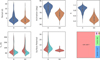 |
Fig. 1 Violin plot showing the distribution of the parameters used in synthetic construction of light curves for detached (D) and semidetached (SD) binaries. The white lines at the centres are the median values covered by black boxes whose lower and upper boundaries are the first and third quartiles, Q1 and Q3 (Krzywinski & Altman 2014). The two ends of the lines overlap with the boxes, denoting the minimum and maximum values of the parameter. The density plots around the boxes represent the probabilities of the corresponding values in the y-axis, where the wider one refers to more frequent occurrences. The effective temperature (Te) and surface potential distributions for the primary (red, left) and secondary (green, right) components are shown in split areas for the sake of a smooth comparison of the values in the two leftmost plots in the bottom pane. We note that the surface potential plot for the semidetached systems only contains values of components well detached from their Roche lobe since the potential of the other component is assumed to be equal to its critical value, indicating that the component fills its Roche lobe. The last box is a treemap plotted based on the number of light curves in different phases of light curve construction. The numbers of detached and semidetached systems from catalogues are 110 and 212 (two small tiles in the upper right). DSYN and SDSYN are synthetic detached and semidetached light curves constructed using the catalogue data, while SYN refers to the total number of synthetic light curves mimicking EBPCs and used in model training and validation. |
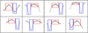 |
Fig. 2 Samples from the synthetic light curve images with the ground truth bounding boxes corresponding to pulsations (red) and minimum (blue) patterns. |
3.3 Observational data
We collected known EBPCs from four main studies: Liakos & Niarchos (2017), Kahraman Aliçavus¸ et al. (2022), Shi et al. (2022), and Kahraman Aliçavuş et al. (2023). The first two and the last one list the systems with δ Sct type components, while the third study catalogues the pulsators in EA-type binaries. The total number of the systems reached 426 after a cross- match based on the target name. The light curve image for a given binary was constructed through a series of steps utilising multiple code snippets. The process began with reading target names from a predefined list of known EBPCs and accessing the Barbara A. Mikulski Archive for Space Telescopes (MAST) database to verify the existence of data files corresponding to the targets. For targets that passed the first step, we performed a target name confirmation process by inspecting the headers of the FITS files to ensure the data belonged to the intended targets. Next, we extracted the TIME and SAP_FLUX values from the FITS files, removing any invalid or NULL data points. The flux values were then converted into magnitudes (mi) using the formula mi = −2.5log Fi, where Fi represents the SAP_FLUX values in the corresponding FITS files. To determine the time intervals for each light curve, the orbital period values from the TEBS catalogue (Prša et al. 2022) were multiplied by a user-defined period factor (in our case, 0.7; see Sect. 2). This ensured that the time-magnitude pairs for each system were tailored to our analysis objectives. Finally, the light curve images were generated by plotting the time-magnitude pairs. The patterns for those images were annotated by hand using LABELIMG3 software. The light curves showing extreme scattering and the ones with unclear patterns were eliminated. We obtained 330 images from observational data through this process; however, the number is still quite small for our aim.
To increase the number of observational data, we divided the light curve of each target into several parts in time by using a certain factor of the orbital period. For instance, seven fits files from the TESS mission meet the conditions when applying a search for the system TIC 48084398 in the MAST portal. The observation durations (Tstop − Tstart) of the data change from 24.86 to 28.20 days, corresponding to a total of 187.04 days long. Dividing the complete observations into equal parts covering 0.7 of the orbital period in time (0.7 × 2.1218069 = 1.48 days, in the case of TIC 48084398) results in data for almost 126 individual light curves for a single system. This method led us to construct thousands of images, but annotating by hand was no longer effective. Therefore, we developed a web implementation, Detection of Oscillations in Eclipsing Binary Light CurveS4 (DetOcS), that reads the fits file of the corresponding target on MAST portal by using Astropy (Astropy Collaboration 2013, 2018, 2022); divides the light curve data in time, relying on the parameter given by the user; constructs light curve images; applies detection; and creates annotation files according to the detection results by using an iterative object detection refinement method. The implementation also allows for fast human confirmation of the detected patterns with one click, considerably easing the data collection procedure. DETOCS contains the above-mentioned code snippets as functions and also requires a pre-trained model. Therefore, we first created a TensorFlow object detection model trained with our synthetic (see Sect. 3.2) and 330 observational light curves by using the most computationally inexpensive model similar to one that is explained in Sect. 4.1. Though we provide details in the next section, we give a brief summary here: when training the object detection model, the network learns to detect and localise objects in images by predicting bounding boxes and class labels in a single pass. In this way, we gathered 1493 observational light curve images with their annotations2, which is more than 4.5 times the initial number. The eight samples directly taken from the output of DETOCS are shown in Fig. 3.
In conclusion, the total number of human-confirmed synthetic and observational light curve image data is 11 370. The data can be accessed online2, with their annotation files in Pascal VOC format. Figure 4 presents all the bounding boxes gathered into a single image, highlighting the effective distribution of annotations across the image area. The minimum and pulsation patterns a achieve coverage of 98.3% and 71.5% of the area, respectively. The dense appearance of the red boxes on the upper part is not unexpected since the pulsation patterns are generally observed at maximum phases. For the reader who becomes curious about why the confirmation by a human is crucial, even for the observational data, we restate the aim of the present computer vision study: to give the machine the ability to see the patterns in the light curves at a level that is at least close to that of an experienced human. Therefore, careful preparation of all images and annotations in datasets are essential.
4 Detection of the pulsation and binarity
For the present study, we employed CNN-based object detection models processing input images. The models first pass the images through a series of convolutional layers, where they automatically learned hierarchical features at different spatial resolutions. In this process, a model extracts the relevant patterns that are essential for identifying objects. Once the features are obtained, the network generates candidate bounding boxes around potential objects in the image. Each bounding box is then classified into predefined object categories, and the model refines the predictions by adjusting the bounding box coordinates to more accurately localise the objects. The final output consists of class labels and their corresponding bounding box coordinates, providing a precise identification and localisation of objects within the image.
We used four conventional and one custom object detection model during the training and detection phases based on two patterns, pulsation and minimum, which are the crucial patterns seen in the light curve of an EBPC. The annotation files for the images (see Sects. 3.2.2 and 3.3) that determine the location and size of the patterns of interest were converted to PASCAL VOC (Everingham et al. 2010) XML format excluding the YOLO model, which requires a specific YOLO format consisting of centre positions, widths, and heights of the ground truth boxes different from the XML format, which is based on the horizontal and vertical coordinates of the box corners.
Of the images constructed from synthetic and observation light curves, 30% were set aside as a validation dataset. Thus, our training set consists of 7959 images, and the number of images in the validation dataset is 3411. One must keep in mind that using the following models on a custom dataset is a pretty complicated procedure, as it includes countless testing of the related parameters and hyperparameters in algorithms. We summarise these procedures in the following sections by giving the results. Additional information about models and the crucial parameters of the training procedures can be found in Appendix B.
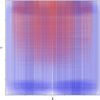 |
Fig. 4 All pulsation (red) and minimum (blue) ground truth bounding boxes in one image area. (See text for details.) |
4.1 Single-shot multi-box detector model
The single-shot multi-box detector (SSD) model (Liu et al. 2016) combines the efficiency of multi-scale feature maps and bounding boxes to detect various sizes of objects. The model uses feature maps in different sizes that allow for the detection of high-level and fine-grained information of images. It can detect multiple objects in various categories with relatively high accuracy and is therefore a preferred model for computer vision tasks.
The object detection algorithm using the SSD method was set in the TensorFlow platform, specifically in TensorFlow Object Detection API5. The model6 forms in SSD algorithm using the MobileNet v2 (Sandler et al. 2018) feature extractor. We first trained the model for 30 minutes and 7 seconds until the 25 000th epoch and observed the detection performance, which was unsatisfactory. Then the model from the last epoch was set as a new fine-tuning checkpoint and re-trained to achieve more quality detections. The re-training process took 14 minutes and 13 seconds until the 6200th epoch. Once the training was complete, we extracted a model file7, and thus we could test the performance of the model at detecting the patterns of interest in the observational light curves of the validation dataset. Using a final model file, the detection took 0.22 seconds per light curve image. The variation of training and validation loss functions through epochs are presented in Fig. 5, with the mean average precision at a 0.5 IoU threshold, mAP (IoU=0.5). Both the training and validation losses decreased steadily as the training progressed, which is a positive sign and indicates that the model is learning from the training data and improving its performance on the validation set. Continuous decrement of loss in the validation set suggests that the model has learned the patterns in the data well and is generalising effectively to the unseen data. A low training and validation loss also indicates that the model is not overfitting and can generalise well. Figure 6 compares detections with the maximum and minimum average IoU values under the condition that the confidence level threshold equals 0.5 within the images where both patterns were detected. The model is quite successful at detecting the patterns covered by ground truth annotations, both for whole validation data and observational images in the validation dataset, as seen in Fig. 7. The figure presents the confusion matrix, which serves as a key tool for assessing model performance by allowing comparison of true labels to predicted labels. It displays the percentage of true positives (correct predictions of the positive class), true negatives (correct predictions of the negative class), false positives (incorrect predictions of the positive class), and false negatives (incorrect predictions of the negative class). This matrix enabled us to assess the overall accuracy while also highlighting the model’s performance for each specific class. As seen in the figure, the percentages of the true positives and true negatives are satisfactorily high, while 0.36% and 0.26% of the observational dataset is identified as background. The ’background’ refers to regions of the image that do not contain any objects of interest, specifically areas that are not annotated with bounding boxes for the target classes in the dataset. When evaluating the model’s performance using a confusion matrix, the background is crucial for determining false positives (incorrectly identified objects in the background), in addition to other performance parameters. The PASCAL (Everingham et al. 2010) and COCO (Lin et al. 2014) evaluation metrics for the model were calculated using the validation data and listed in Table 2. The precision-recall curves for different IoU thresholds are shown in Fig. 8, which indicates an expected decrement in recall for increasing precision. In this context, the precision measures the proportion of true positives among all predicted positives, while recall measures the proportion of true positives detected out of all actual positives. An ideal precision-recall curve for an object detection model should have a high area under the curve, with both precision and recall values remaining consistently high across different decision thresholds, such as IoU values. In a perfect model, precision would remain high even as recall increases, indicating that the model detects most objects without generating false positives. However, in real-world models, precision typically decreases as recall increases. The goal is to achieve a curve that stays high and thus reflects strong precision even when recall is high, which indicates a good balance between detecting true positives and avoiding false positives. This balance is critical in object detection tasks for maintaining accurate predictions. Everingham et al. (2010) provided an overview of precision and recall evaluation metrics in object detection tasks, especially within the framework of Pascal VOC, which have been widely used to benchmark object detection models. In the figure, the final precision also decreases in higher IoU values. The minimum patterns seem easy to be detected compared to the pulsation patterns, which show more diversity in their shapes.
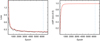 |
Fig. 5 Loss and mAP variation for the SSD model during training and evaluation. The black and red lines refer to training and validation values, respectively. The blue dashed line corresponds to the 6200th epoch, the step for the final model. The plot data was smoothed exponentially by a factor of 0.6 to emphasise the trend. The TensorBoard parameter plots are available in the provided Google Colab notebook8. |
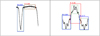 |
Fig. 6 Samples of different detection performances on observational light curve images in the validation set with a predicted bounding box for each ground truth annotation for the SSD model. Detected patterns (in red and blue bounding boxes) with the maximum (left, TIC 73672504) and minimum (right, TIC 232637376) average IoU values are compared to ground truth annotations (green dashed boxes). The numbers above the boxes correspond to the IoU value for the related detection. The letters P and M refer to pulsation and minimum patterns, respectively. |
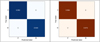 |
Fig. 7 Confusion matrices for the overall (left) and only the observational (right) data in the validation dataset calculated based on the predicted class and bounding boxes by setting the IoU and confidence level to 0.5. We note that 0.08% of pulsation and 0.41% of the minimum patterns were detected as background, namely, predicted as though they are not objects of interest for the overall data, while the percentages are 0.36% and 0.26% for observations. The letters P and M refer to pulsation and minimum patterns, respectively. |
PASCAL and COCO evaluation metrics from detection on the validation set using different models.
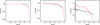 |
Fig. 8 Precision-recall curves of the detection in IoU=0.5 (left), IoU=0.75 (middle), and IoU=0.9 (right) thresholds. The black and red lines correspond to minimum and pulsation patterns, respectively. The calculations were conducted by using the code given by Padilla et al. (2021). |
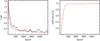 |
Fig. 9 Variation of loss and mAP across epochs for the Faster R-CNN model. The black and red lines represent training and validation values, respectively, while the blue dashed line indicates the epoch corresponding to the final model. The TensorBoard parameter plots are available in the accompanying Google Colab notebook8. |
4.2 Faster Region-based CNN model
The Faster Region-based CNN (Faster R-CNN; Ren et al. 2017) is another effective model for object detection tasks in computer vision. It builds based on its predecessors, R-CNN (Girshick et al. 2014) and Fast R-CNN (Girshick 2015), by using a region proposal network (RPN; Ren et al. 2015) that significantly speeds up object detection.
Training until the final epoch, 4600th, lasted 25 min and 28 sec on one Nvidia GeForce RTX 2080 Ti accelerator. The decrement of the total loss function, which is the sum of localisation, classification, and objectness losses, during training and evaluation is shown along with the mean average precision in Fig. 9. Even the selection of small batches shows itself with fluctuations in the curve. The decrement is smooth, and further critical improvement was not observed in the following epochs. The validation loss value is close to the training at the 4600th epoch, which corresponds to the final model’s ability to generalise the unseen data. Detections were conducted using the final model file7, which takes 0.07 seconds per frame, and the samples of inferences with the highest and lowest average IoU values are shown in Fig. 10. The model does appear to detect patterns where pulsations are superposed on the minimum pattern (right panel) similar to SSD, although the IoU values are around 0.7. The PASCAL and COCO metrics of the detection are presented in Table 2. The percentage of correctly predicted detections is shown in Fig. 11 for the complete dataset and observations, separately, which are above 99% for three classes. The precision-recall curves (Fig. 12), on the other hand, indicate that the model performance decreases with increasing IoU threshold, as expected.
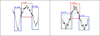 |
Fig. 10 Examples of varying detection performance of the Faster R-CNN model on observational light curve images from the validation set displaying predicted bounding boxes for each ground truth annotation. The detected patterns (in red and blue bounding boxes) with the highest (left, TIC 158794976) and lowest (right, TIC 232637376) average IoU values are compared against ground truth annotations (green dashed boxes). The numbers above each box indicate the IoU value for the corresponding detection. The letters P and M denote pulsation and minimum patterns, respectively. The yellow box on the right panel represents the additional detection that is not present in the ground truth annotations. |
 |
Fig. 11 Confusion matrices for the overall data (left) and observational data only (right) in the validation dataset calculated using predicted class and bounding boxes, with the IoU and confidence threshold set to 0.5 with the Faster R-CNN model. The letters P and M denote pulsation and minimum patterns, respectively. |
4.3 You Only Look Once model
The You Only Look Once (YOLO) model (Redmon et al. 2016) uses a unique methodology that is different from the two-step methods conventionally shown in regional scanning techniques. The YOLO model runs based on dividing the input image into parts and estimates the bounding boxes and class probabilities for a detected pattern within the individual parts. The advantage of the YOLO’s methodology lies in its speed and accuracy. The algorithm has wide usage areas in various disciplines.
During the training process, we employed YOLOv5s architecture (a compact version within the YOLOv59 family designed to offer faster inference times while maintaining reasonable accuracy) together with the pre-trained weights. The training and validation losses decreased very smoothly by increasing steps (Fig. 13), and no improvements were observed after the 57th epoch, the step where the final model7 was extracted. The loss function in the figure is the total loss, which is the summation of three losses: box loss, class loss, and objectness loss. The training process lasted 5 hours and 43 minutes, substantially longer compared to other models. The model can be considered as showing a very good performance in detection patterns in the validation dataset, which can be seen in Fig. 14, where the detections with maximum and minimum average IoU values are shown. Contrary to the long training process, the detection over 3411 images took 33.92 seconds, averaging approximately 0.01 seconds per image, the best performance among all our models. The accurate detection of the model, even for the observational data, can be seen in the confusion matrices in Fig. 15, where the results are close to those of Faster R-CNN. The precision-recall curves of the model for different IoU values show consistent variation compared to all other models in the study, as given in Fig. 16. The shapes underscore the model’s robustness in balancing precision and recall effectively, even under different IoU settings (as we remarked in Sect. 4.1). The resulting metrics of the detection are listed in Table 2.
4.4 EfficientDet D1 model
The EfficientDet model (Tan et al. 2020) combines various techniques to achieve high accuracy and efficiency simultaneously. The balance between accuracy and computational efficiency complies with a wise usage of the scaling method, optimising model architecture, resolution, and input size.
We applied two consecutive training procedures similar to the one mentioned in Sect. 4.1. The retraining process lasted 23 minutes and 25 seconds, corresponding to 7100 epochs. The detection per frame took 0.58 seconds using the final model file7, the longest time of any model. The training and validation loss through the epoch number is shown in Fig. 17 with the mAP values. The prominent fluctuations in the training curve arise from the small batch size mentioned previously. The loss values beyond the 7100th epoch tend not to improve in the following epochs. On the other hand, mAP(Iou=50) exceeds 0.9. The detections with maximum and minimum average IoUs are plotted in Fig. 18, where values around 0.5 can be seen. The confusion matrices are given in Fig. 19, while the related metrics are listed in Table 2. The model performed relatively weakly in detecting all the minimum patterns, whereas it successfully predicted more than 90% of the pulsation patterns in observational data. The precision-recall curves for various IoUs are also presented in Fig. 20. An irregular trend and a large amount of decrement in precision for the minimum pattern with the increasing IoU threshold is clear. It is worth emphasising that we tried the previous lighter member, EfficientDet D0; however, the results, especially the decrement in the cost function, were not as satisfactory as expected from an EfficientDet family model.
 |
Fig. 12 Precision-recall curves for the Faster R-CNN model at IoU thresholds of 0.5 (left), 0.75 (middle), and 0.9 (right). The black and red lines represent the minimum and pulsation patterns, respectively. |
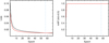 |
Fig. 13 Plot showing the loss and mAP as they change with increasing epochs for the YOLO model. The black and red lines represent training and validation values, respectively, and the blue dashed line marks the epoch of the final model. The TensorBoard parameter plots are available in the provided Google Colab notebook8. |
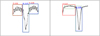 |
Fig. 14 Different detection performances on observational light curve images from the validation set showing predicted bounding boxes for each ground truth annotation using the YOLO model. The detected patterns, enclosed in red and blue boxes, with the highest (TIC 354922610, left) and lowest (TIC 323292655, right) average IoU values are compared to the ground truth annotations marked by green dashed boxes. The numbers above each box indicate the IoU value for that detection. The letters P and M represent pulsation and minimum patterns, respectively. |
4.5 A non-pretrained CNN-based model
We implemented a CNN-based object detection model from scratch that is not based on a pre-trained architecture in order to compare its performance with pretrained models and see if our task can be carried out faster and more effectively with a simpler model consisting of CNNs. The model1 algorithm was set to be able to read two classes per image; therefore, our annotation files10 include ground truths of two patterns for each image.
The training lasted 2 hours and 24 minutes on the same accelerator mentioned earlier. The best model7 was achieved in the 93rd epoch, where the train and validation losses are almost at their minimum without significant overfitting. The learning curves are presented in Fig. 21, where the loss is the summation of classification and box regression losses. The curves exhibited a consistent improvement in both loss and accuracy metrics. The accuracy of the box predictor, which achieves a plateau at about 0.9, is also plotted in the figure. A steep decline in both the training and validation loss was accompanied by a steady rise in accuracy, indicating effective learning. The model infers 3411 validation data in 315.65 seconds, corresponding to almost 0.09 seconds per frame. The predictions are noticeably weaker than the previous models such that no detections occur with the average IoU value exceeding 0.8. The metrics obtained from the detections are also listed in Table 2. The detections with maximum and minimum average IoU values are illustrated in Fig. 22. The low quality of the detections can also be seen from the confusion matrices (Fig. 23) for the entire data and for only the observational data, separately demonstrating that the model detected a huge amount of the patterns as background. The precision-recall curves for three IoU thresholds are also given in Fig. 24, and they indicate that the increasing threshold value dramatically changes the curve such that it ends up with small precision and recall values.
We applied detections to the data with the highest and lowest IoUs from each model using the four other models (Figs. 25 and C.1–C.4) in order to provide a clear comparison of the results. In reviewing the nine light curves used in this procedure, we found the overall average IoU values to be 0.83, 0.79, 0.76, 0.67, and 0.22 for the SSD, Faster R-CNN, YOLO, EfficientDet D1, and non-pretrained CNN-based models, respectively. Although IoUs vary depending on the pattern occurrence within images, the pre-trained models clearly demonstrated their precision in this comparison.
 |
Fig. 15 Confusion matrices for the overall data (left) and observational data (right) in the validation dataset derived based on predicted classes and bounding boxes using the YOLO model, with IoU and confidence threshold set at 0.5. The letters P and M stand for pulsation and minimum patterns. |
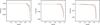 |
Fig. 16 Precision-recall curves of the YOLO model illustrated for IoU thresholds of 0.5 (left), 0.75 (middle), and 0.9 (right). The minimum patterns are indicated by the black line, while pulsation patterns are indicated by the red line. |
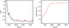 |
Fig. 17 The decrement in Loss and mAP with increasing epochs for the EfficientDet D1 model is illustrated. The black and red lines denote training and validation values, respectively. The blue dashed line marks the final model at the 7100th epoch. TensorBoard parameter plots are available in the provided Google Colab notebook8. |
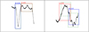 |
Fig. 18 Examples of detection performance variation of the EfficientDet D1 model on observational light curve images from the validation set, featuring predicted bounding boxes for each ground truth annotation. Detected patterns, highlighted in red and blue boxes, with the highest (left, TIC 350030939) and lowest (right, TIC 355151781) average IoU values are compared to the ground truth annotations shown in green dashed boxes. The numbers above the boxes represent the IoU values for each detection. The letters P and M stand for pulsation and minimum patterns, respectively. |
 |
Fig. 19 Confusion matrices for the overall dataset (left) and only the observational data (right) in the validation set. The matrices were generated based on predicted classes and bounding boxes using the EfficientDet D1 model and by setting an IoU and confidence threshold of 0.5. We consider that 0.1% and 0.6% of the minimum patterns are misclassified as pulsation for the overall (left) and observational data (right), respectively. The letters P and M denote pulsation and minimum patterns. |
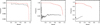 |
Fig. 20 Precision-recall curves for the EfficientDet D1 model at IoU thresholds of 0.5 (left), 0.75 (middle), and 0.9 (right). The black line corresponds to minimum patterns and the red line to pulsation patterns. |
5 Test on Kepler data
The complete procedure mentioned above was conducted using TESS light curve data. It is, however, crucial to use another database to test the model performance regarding the unseen data of different sources and check the usability with other datasets. For this purpose, Kepler light curve data, especially those taken in short cadence, are very appropriate. Using the models with the best results, namely SSD, Faster R-CNN, and YOLO, we applied the test to the Kepler short cadence data of 124 systems with δ Sct type pulsating components, whose KIC numbers are given by Liakos & Niarchos (2017). It must be emphasised that we did not cross-match the Kepler stars with our TESS targets since the purpose was to test the inference performance using a different database and the number of known systems is rather low. Among the 124 systems, 40 have short-cadence data with the object ID in the FITS header matching the KIC numbers of the systems in the test set. The procedure described in Sect. 3.3 was used to construct the light curve images. A modified version of DETOCS, detocs_k.py4, was used during the test with two models, SSD and Faster R-CNN. Testing on the Kepler dataset using the YOLO model, on the other hand, was conducted by employing the corresponding inference code9. The confidence threshold was set to 0.5 during the procedures.
Table C.1 lists the detection results showing the maximum average confidence values (sum of confidences divided by the number of detected patterns) for the systems with the model used in the detections where Faster R-CNN dominates with the highest values. Both pulsation and minimum patterns were detected in 36 targets out of 40 by SSD, 38 by Faster R-CNN, and 35 by YOLO. Figures C.5, C.6, and C.7 illustrate the detections with the largest average confidence values for each target. The confidence scores displayed above the corresponding boxes in the light curves are designed to reflect the model’s certainty in its predictions. Bounding boxes with lower confidence scores, as seen in some detections such as KIC 4480321, KIC 4544587, and KIC 9470054 in SSD and Faster R-CNN models, indicate that the model is less certain of the prediction. These low-confidence results should be interpreted with caution, as they hold less significance compared to high-confidence predictions. The systems shown in the figures are those with the highest average scores rather than the highest individual scores, as the selection process prioritised the average due to the presence of two classes of patterns. Another reason for focusing on detections with the highest average confidence scores is that we did not consider the total number of patterns or their locations. Detecting a single pulsation pattern along with the minimum, having a high confidence score – regardless of its position in the image – is sufficient to indicate that the system is a potential EBPC candidate. The different light curve shapes of the same target for different models in the figures arises from the result that the models detect patterns with the highest confidence in the image constructed using different time intervals for a given target (see Sect. 3).
We also attempted to apply the detection of pulsation and minimum patterns in the light curves of Kepler eclipsing binary systems listed in Matijevič et al. (2012). Although the catalogue consists of several parameters besides the orbital periods of 2920 systems, we managed to access short-cadence Kepler data of 574 binaries. The same detection procedure explained above was conducted, but on this occasion, we only used Faster R-CNN, as it is the model that showed the highest confidence scores in our previous detection experience. Since many of the systems are not EBPCs in the catalogue, the model detected only minimum patterns in the vast majority of the images. Figure C.8 displays the light curves that exhibit both pulsation and minimum patterns in eclipsing binaries with appropriate data from the catalogue. For this particular figure, instead of using the average confidence score for pulsation and minimum patterns, as is generally done, we chose to highlight the light curves with the 25 highest confidence scores for pulsation patterns in order to emphasise the most prominent cases of pulsation in the dataset. As seen in the figure, the model also treated certain scatterings as pulsations in some images. This behaviour may arise due to the noise-like appearance of real pulsations in the light curves of some known EBPCs in our training set, where the relatively high-frequency oscillations are hardly distinguishable in the selected time interval. Therefore, to be on the safe side, those detections should not be considered pulsations without confirmation by further analysis. As an outline, the results indicate that the model has a promising ability to eliminate large amounts of light curves that are not showing two patterns together, namely those that are not potentially EBPCs. It is also capable of detecting the patterns of interest correctly very fast; however, a final human inspection is still needed to confirm that a given system is an EBPC.
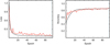 |
Fig. 21 Learning curves for the non-pretrained CNN model. Left: variation of loss over epochs. Right: accuracy of the box predictor as training progresses. The black and red lines represent training and validation values, respectively, with the blue dashed line marking the epoch of the final model. |
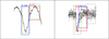 |
Fig. 22 Samples of detection performance on observational light curve images from the validation set displaying predicted bounding boxes for each ground truth annotation for the non-pretrained CNN model. The detected patterns, shown in red and blue boxes, with the highest (left, TIC 298734307) and lowest (right, TIC 409934330) average IoU values are compared to the ground truth annotations, marked by green dashed boxes. The numbers above each box represent the IoU value for the respective detection. The letters P and M denote the pulsation and minimum patterns, respectively. |
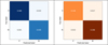 |
Fig. 23 Confusion matrices for the overall data (left) and the observational data (right) in the validation set. The matrices were computed based on predicted classes and bounding boxes, with the IoU and confidence thresholds set to 0.5 and using the non-pretrained CNN-based model. We note that the model is considerably unsuccessful at detecting patterns, especially on observational data. The letters P and M denote pulsation and minimum patterns, respectively. |
 |
Fig. 24 Precision-recall curves for the non-pretrained CNN model plotted with IoU thresholds of 0.5 (left), 0.75 (middle), and 0.9 (right). The black line denotes the minimum, and the red line indicates pulsation patterns. We note that the recall axis is shortened in the rightmost plot for better visibility. |
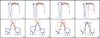 |
Fig. 25 Detection performance of Faster-RCNN (a1, a2), YOLO (b1, b2), EfficientDet D1 (c1,c2), and non-pretrained CNN-based (d1, d2) models on the light curves in Fig. 6. |
Overview of object detection models used in the study.
6 Results and conclusion
We have presented efforts to detect certain shapes similar to the effect of pulsation in eclipsing binary light curves by using conventional CNN-based object detection algorithms and a custom one. The synthetic and observational light curve images forming our dataset were used to train the models and validate their performance. Table 3 summarises the key properties of the models used in this study, including the changes made to align with our objectives. Several codes, accessible via the internet1, were written to conduct the procedures more autonomously. A web implementation, DETOCS, was also developed to apply inference based on certain models and to increase the number of samples in the dataset using the refinement method. This approach allows the user to detect patterns of interest by entering a set of parameters, which means it can be used to discover new candidates in the future.
Our results indicate that the Faster R-CNN shows the best performance to unseen data (Table C.1) among the models introduced in the present study. The metrics obtained from SSD were also sufficient, which makes it useful considering its speed in training and at detecting patterns. YOLO is the fastest at detecting targets and resulted in a very good performance (Table 2); however, it was slow in the training process compared to the other models. The EfficientDet D1 model showed the lowest performance in training and inference regarding speed and accuracy, but its results are adequate, as it correctly detected almost 90% of the patterns in the observational light curves in the validation set. In general, three of our models can be considered successful at detecting oscillation-like and minimum-shaped patterns in more than 94% of the observational eclipsing binary light curve data. The custom CNN model is the weakest one, which lets us consider that a non-pretrained model may not be powerful enough to achieve the desired number of successful detections. A histogram of the average IoU values obtained by the models is plotted in Fig. 26. The IoUs are considerably high and even exceed 0.9 for pre-trained models, SSD, Faster R-CNN, YOLO, and EfficientDet D1, while they are gathered in the region of the low values for the non-pretrained CNN-based model. The figure indicates that the values also peak at a 0.8–0.9 interval for the four models. When evaluating the results concerning precision-recall curves, YOLO comes to the forefront in all IoU thresholds considering the consistency of the curve, as discussed in Sect. 4.1, where we explained the ideal properties of the curve, including maintaining high precision and recall across different decision thresholds. It is followed by the Faster R-CNN and SSD models with substantial trends, especially at IoU values of 0.5 and 0.75. Given the outcomes from the different phases of our study, the results clearly show that pre-trained conventional models work considerably better in the present task, detecting the patterns of interest with satisfactory results. A further detection with the Faster R-CNN model was also applied to the light curves of Kepler eclipsing binary systems with short-cadence data. The results indicate that 68 systems show an oscillationlike pattern in their light curves after human inspection of the inferences was conducted. Figure C.9, a continuation of Fig. C.6, shows the detected patterns in the light curves of 30 systems with the highest average confidence scores, excluding the 38 known EBPCs presented earlier. The variability types that may be responsible for the detected light variations, as provided in the literature, are listed in Table C.2.
To summarise, the performances of the models indicate that the object detection approach has the potential to scan the light curves and detect new eclipsing binary candidates with pulsating components in the present and future space- and ground-based missions. The data from different databases can be accessed and shaped in a suitable form almost autonomously by using the series of codes we have presented. The model DETOCS can also be used to conduct detections in various databases with a few modifications based on the accessed data source. The method is considerably fast at detecting patterns, as the elapsed time for detection per image takes less than half a second when using our model files, as mentioned in previous sections.
As a subsequent step to the present work, we plan to apply the trained object detection models on all available TESS and Kepler datasets to identify more EBPCs. Given these databases’ huge quantity and complexity, this will be a challenging task that will require careful organisation. However, our methods have demonstrated the ability to rapidly detect targets, even in relatively large and complex data. This efficiency will be particularly beneficial as we scale up to the full datasets, enabling us to infer potential targets much faster than traditional methods. We anticipate that optimising model performance on this larger scale will involve iterative tuning of parameters, such as time intervals and confidence scores. Nonetheless, the code and methodologies have prepared us to handle these challenges with confidence. This extended application will validate our models, increase the number of potential EBPC candidates, and uncover new insights within the datasets. Furthermore, more accurate data from future missions, such as PLATO (Rauer et al. 2014), will also provide a vast playground for applying and fine-tuning our models. Alternatively, similar object detection models can be trained to detect other patterns or shapes corresponding to a variety of astrophysical phenomena in order to discover new targets of interest for in-depth examination.
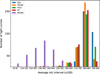 |
Fig. 26 Histogram showing the distribution of average IoU values achieved in detecting patterns on the observational light curves in which both classes (P and M) are detected. The numbers in the box brackets refer to the value intervals. The term ‘Eff’ stands for EfficientDet D1 model. |
Acknowledgements
BU acknowledges the financial support of TUBITAK (The Scientific and Technological Research Council of Turkey) within the framework of the 2219 International Postdoctoral Research Fellowship Program (No. 1059B192202496). Hospitality of the HUN-REN CSFK Konkoly Observatory is greatly appreciated. RSz and TSz acknowledge the support of the SNN-147362 grant of the Hungarian Research, Development and Innovation Office (NKFIH). The numerical calculations reported in this paper were partially performed at TUBITAK ULAKBIM, High Performance and Grid Computing Center (TRUBA resources). This paper includes data collected with the TESS mission, obtained from the MAST data archive at the Space Telescope Science Institute (STScI). Funding for the TESS mission is provided by the NASA Explorer Program. STScI is operated by the Association of Universities for Research in Astronomy, Inc., under NASA contract NAS 5–26555. This paper includes data collected by the Kepler mission and obtained from the MAST data archive at the Space Telescope Science Institute (STScI). Funding for the Kepler mission is provided by the NASA Science Mission Directorate. STScI is operated by the Association of Universities for Research in Astronomy, Inc., under NASA contract NAS 5–26555. This work made use of Astropy (http://www.astropy.org): a community-developed core Python package and an ecosystem of tools and resources for astronomy (Astropy Collaboration 2013, 2018, 2022). This research has made use of the SIMBAD database, operated at CDS, Strasbourg, France. The authors acknowledge OpenAI’s ChatGPT for its assistance in debugging certain codes used in this research, with all suggested corrections carefully reviewed and validated by the authors before implementation.
Appendix A Formulation for parameter determination
We present the formulae and assumptions used in parameter determination for eclipsing binaries during the construction of synthetic light curves. The catalogues mention in Sect. 3.2.1 (Southworth 2015; Malkov 2020) lists the effective temperatures  , orbital period of the systems (P), masses (M1, M2), and radii (R1, R2) of the components.
The mass ratio (q) was calculated using the formula  by assuming that the M1 is more massive than M2 for semidetached binaries. The surface potential of the primary component was determined using the modified Kopal potential (Kopal 1959), under the assumption of synchronous rotation:

where r1 is the fractional radius,  , with a being the separation calculated using Kepler’s third law,
  , and the corresponding assumptions. Furthermore, λ = sin θ cos ϕ and v = cos θ, where θ and ϕ are the polar and azimuthal angles, respectively. Ω1 was derived for doublets of (λ, v) and remains constant over the surface.
The surface potential of the secondary component was then derived as

The inclination, i, was determined under the assumption that for an eclipse to occur the projected separation (a sin i) must be less than or equal to the sum of the radii of the stars, a sin i ⩽ R1 + R2 and therefore, sin  which corresponds to the following using sin2i + cos2 i = 1:

Considering the inclination is between [0°, 90°] and thus the positive root, the following can be written as

which was set as the minimum value in our study. It was increased following the method explained in Sect. 3.2.1.
Appendix B Model specifications
We provide additional information about the specifications, the operational steps of models and the key parameters/hyperparameters necessary for their successful execution and satisfactory performance in the following subsections.
B.1 Single-shot multi-box detector model
The steps involved in the SSD detection process are as follows. The SSD model begins by accepting an input which resizes to a certain size and normalises for consistency. It uses a backbone network, MobileNet v2 in our case, to extract feature maps from the image. These feature maps represent the input at multiple scales, enabling the detection of objects of varying sizes. SSD divides the feature map into a grid and assigns each cell multiple default bounding boxes with varying aspect ratios. Each default box predicts a confidence score for every class and refines its location. Finally, SSD applies non-maximum suppression (NMS; Redmon et al. 2016) to remove overlapping boxes with lower confidence scores, resulting in the final bounding boxes, confidence scores, and class labels.
The model contains a predefined anchor box used to estimate the bounding boxes and class probabilities. The most important feature of the SSD is the capability to set a balance between detailed spatial patterns and high-level semantic patterns, which lets the algorithm detect objects with diverse characteristics. The relatively fast estimations of the method spread its usage for various aims like object detection in complex scenarios. Our model was SSD algorithm with MobileNet backbone which is pre-trained on the Common Objects in Context 2017 (COCO; Lin et al. 2014). It combines the efficiency of MobileNet v2 architecture with the accuracy of the SSD framework. Its structure is compact and requires low computational power. Working on moderate resolution sets the model to balance speed and precision. The data record files, label maps and a pipeline configuration file, which are crucial for training, were created using the API’s related codes.
Several series of batch_size, warmup_learning_rate and learning_rate_base parameters were examined by considering the commonly used values for SSD models. Eventually, our final model in re-training yielded by fine-tuning these values as 32,0.0001 and 0.0005, respectively. The L2 regularisation (Rumelhart et al. 1986) was also added by setting its weight to 0.00006. The different step size values were also tried. We concluded that the model in the 6200th epoch is the most optimal value for the parameter (num_step) to avoid overfitting in the retraining process as there was no significant improvement in validation loss and its difference from the training loss during the next steps of training. The complete process was conducted on the Malor server of Konkoly Observatory using one Nvidia GeForce RTX 2080 Ti accelerator. The loss function was selected as a combination of classification and localisation losses which are sigmoid and smooth L1 loss functions, along with the regularisation loss. Using the final model it took 771.75 seconds to detect patterns on 3411 validation images.
B.2 Faster Region-based CNN model
Faster R-CNN starts by processing an input image of arbitrary size, normalising its pixel values before feeding it into a backbone network (ResNet50 V1; Lin et al. 2014). The backbone extracts feature maps, which are passed to the RPN. The RPN scans the feature maps to generate region proposals, identifying areas likely to contain objects. These proposals are then aligned with the feature map using ROI (Region of Interest) pooling, producing fixed-size feature maps for each region. Finally, these feature maps are used to classify the object in each region and refine the bounding box coordinates. The model outputs the final bounding boxes, confidence scores, and class labels.
The model was pre-trained on the COCO 2017 dataset and accessible through the internet6. The TensorFlow Object Detection API was used during the process, similar to done in the previous section. batch_size was set to four, which dispersed the loss curve slightly; however, no memory overflow was observed during training in return. In the final model, warmup_learning_rate was equal to 0.0001 until the 2000th epochs while learning_rate_base was adapted to 0.001. One Nvidia GeForce RTX 2080 Ti accelerator was used during the procedure.
B.3 You Only Look Once model
The YOLO detection process operates as follows. The model divides the input image into a grid, resizes it, and normalises its pixel values. Each grid cell is responsible for predicting bounding boxes and their associated class probabilities. YOLO employs a deep convolutional neural network to extract features and capture relationships between objects. It performs object localisation, classification, and confidence score prediction in a single forward pass. Each prediction includes bounding box coordinates, a confidence score indicating the likelihood of an object, and probabilities for all possible classes. Finally, NMS is applied to remove overlapping boxes, resulting in the final bounding boxes, confidence scores, and class labels.
Since the model needs fine-tuning to detect our specific objects of interest, similar to previous ones, the size was modified by setting the parameters of the depth_multiple and width_multiple to 0.5. The learning_rate was 0.001 while the weight decay (weight_decay) of the Stochastic Gradient Descent (LeCun et al. 2015) optimiser was adopted to 0.001, a larger value from the default. The only non-zero augmentation parameter was image translation (translate = 0.1), besides default HSV augmentations. A PyTorch-implemented version of the YOLO was used by aiming a leverage in GPU acceleration and automatic differentiation. The training procedure was applied using a 2 x Nvidia GeForce RTX 2080 Ti accelerator.
B.4 EfficientDet D1 model
EfficientDet-D1 processes an input image by resizing it to match the model’s requirements and normalising its pixel values. It uses EfficientNet (specifically the B1 variant in our case) as its backbone for feature extraction, followed by the Bidirectional Feature Pyramid Network (BiFPN; Tan et al. 2020), which merges multi-scale features to improve detection performance. Anchor boxes are generated at multiple scales and aspect ratios, enabling the model to predict objects of different sizes. Each anchor box predicts class probabilities and bounding box offsets. EfficientDet-D1 applies NMS to filter overlapping predictions, producing the final bounding boxes, confidence scores, and class labels. The D1 sub-model has increased detection performance in terms of balance between model size and speed.
The training was made using TensorFlow Object Detection API and related files in the zoo6. The first train process using a pre-trained model showed no improvement in loss functions beyond the 10000th epoch (33 minutes 32 seconds) and resulted in a small number of correctly detected samples in the validation dataset based on the model from the last epoch. Therefore, we retrained the model using the last obtained checkpoint from the initial training. To avoid the extreme load on GPU memory and fail in memory allocation, we set the batch_size parameter to four. A learning rate scheduler was set by adopting warmup_learning_rate and learning_rate_base parameters to 0.0001 and 0.001, respectively, while the weight of the L2 regulariser was adopted to 0.00004. The same accelerator, one Nvidia GeForce RTX 2080 Ti, was used during training and evaluation processes.
B.5 A non-pretrained CNN-based model
The model mainly consists of a convolutional part for extracting features, a dense head to convert feature maps into a 2D vector, three fully connected layers for classification, box regression, and determining confidence. The feature extraction has three convolutional layers with the 16, 16 and 32 filters beside L2 regulariser in the first one. The network consists of 17 hidden layers, with 12 originating from the feature extraction component and 5 from the dense processing stage. The Adam (Kingma & Ba 2015) was used as an optimiser with an initial learning rate of 0.0005, although a learning rate scheduler (ReduceLROnPlateau) was applied to reduce it when validation loss stopped improving. Early stopping callback was also employed based on the validation loss to prevent overfitting; hence, it stopped the training process at the 97th epoch since the value did not improve in the last ten epochs.
Appendix C Supplementary tables and figures
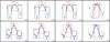 |
Fig. C.1 Same as Fig. 25 but for the detection performance of SSD (a1, a2), YOLO (b1, b2), EfficientDet D1 (c1,c2) and non-pretrain CNN-based (d1, d2) models on the light curves in Fig. 10. |
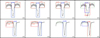 |
Fig. C.2 Same as Fig. 25 but for the detection performance of SSD (a1, a2), Faster-RCNN (b1, b2), EfficientDet D1 (c1,c2) and non-pretrain CNN-based (d1, d2) models on the light curves in Fig. 14. |
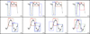 |
Fig. C.3 Same as Fig. 25 but for the detection performance of SSD (a1, a2), Faster-RCNN (b1, b2), YOLO (c1,c2) and non-pretrain CNN-based (d1, d2) models on the light curves in Fig. 18. |
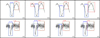 |
Fig. C.4 Same as Fig. 25 but for the detection performance of SSD (a1, a2), Faster-RCNN (b1, b2), YOLO (c1,c2) and EfficientDet D1 (d1, d2) models on the light curves in Fig. 22. |
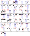 |
Fig. C.5 Mosaic of 36 detections with the highest average confidence scores on short cadence Kepler data of 40 targets using the SSD model. The values above the red and blue bounding boxes refer to the confidence of pulsation (P) and minimum (M) patterns. |
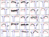 |
Fig. C.8 Same as Fig. C.5 but for the light curves of the systems having the highest 25 confidence scores of pulsation patterns. Be aware that the inference results are contaminated by large scatterings in maximum phases of some light curves. See text for details. |
Maximum confidence scores for detected patterns on the light curves of 40 known EBPCs with a short cadence Kepler data.
References
- Abdallah, Z. S., Du, L., & Webb, G. I. 2017, Data Preparation (Boston, MA: Springer US), 318 [Google Scholar]
- Andersen, J. 1991, A&A Rev., 3, 91 [Google Scholar]
- Angus, R., Morton, T., Aigrain, S., Foreman-Mackey, D., & Rajpaul, V. 2018, MNRAS, 474, 2094 [Google Scholar]
- Armstrong, D. J., Gamper, J., & Damoulas, T. 2021, MNRAS, 504, 5327 [NASA ADS] [CrossRef] [Google Scholar]
- Astropy Collaboration (Robitaille, T. P., et al.) 2013, A&A, 558, A33 [NASA ADS] [CrossRef] [EDP Sciences] [Google Scholar]
- Astropy Collaboration (Price-Whelan, A. M., et al.) 2018, AJ, 156, 123 [Google Scholar]
- Astropy Collaboration (Price-Whelan, A. M., et al.) 2022, ApJ, 935, 167 [NASA ADS] [CrossRef] [Google Scholar]
- Balona, L. A., Baran, A. S., Daszynska-Daszkiewicz, J., & De Cat, P. 2015, MNRAS, 451, 1445 [CrossRef] [Google Scholar]
- Bódi, A., & Hajdu, T. 2021, ApJS, 255, 1 [CrossRef] [Google Scholar]
- Borkovits, T., Derekas, A., Kiss, L. L., et al. 2013, MNRAS, 428, 1656 [NASA ADS] [CrossRef] [Google Scholar]
- Borucki, W. J., Koch, D., Basri, G., et al. 2010, Science, 327, 977 [Google Scholar]
- Brewer, L. N., Sandquist, E. L., Mathieu, R. D., et al. 2016, AJ, 151, 66 [NASA ADS] [CrossRef] [Google Scholar]
- Bromley, B. C., Leonard, A., Quintanilla, A., et al. 2021, AJ, 162, 98 [NASA ADS] [CrossRef] [Google Scholar]
- Čokina, M., Maslej-Krešňáková, V., Butka, P., & Parimucha, Š. 2021, Astron. Comput., 36, 100488 [CrossRef] [Google Scholar]
- Davenport, J. R. A. 2016, ApJ, 829, 23 [Google Scholar]
- Debosscher, J., Blomme, J., Aerts, C., & De Ridder, J. 2011, A&A, 529, A89 [NASA ADS] [CrossRef] [EDP Sciences] [Google Scholar]
- Debosscher, J., Aerts, C., Tkachenko, A., et al. 2013, A&A, 556, A56 [NASA ADS] [CrossRef] [EDP Sciences] [Google Scholar]
- Everingham, M., Gool, L. V., Williams, C. K. I., Winn, J. M., & Zisserman, A. 2010, Int. J. Comput. Vis., 88, 303 [CrossRef] [Google Scholar]
- Gaulme, P., & Guzik, J. A. 2019, A&A, 630, A106 [NASA ADS] [CrossRef] [EDP Sciences] [Google Scholar]
- Girshick, R. B. 2015, in Proceedings of the IEEE International Conference on Computer Vision (ICCV), IEEE, 1440 [Google Scholar]
- Girshick, R. B., Donahue, J., Darrell, T., & Malik, J. 2014, in Proceedings of the IEEE Conference on Computer Vision and Pattern Recognition (CVPR), IEEE, 580 [Google Scholar]
- Guo, Z., Gies, D. R., & Fuller, J. 2017, ApJ, 834, 59 [Google Scholar]
- Hartman, J. D., Bakos, G., Stanek, K. Z., & Noyes, R. W. 2004, AJ, 128, 1761 [NASA ADS] [CrossRef] [Google Scholar]
- Healy, B. F., Coughlin, M. W., Mahabal, A. A., et al. 2024, ApJS, 272, 14 [NASA ADS] [CrossRef] [Google Scholar]
- Kahraman Aliçavus, F., Gümüs, D., Kırmızıtas, Ö., et al. 2022, Res. Astron. Astrophys., 22, 085003 [CrossRef] [Google Scholar]
- Kahraman Aliçavuş, F., Çoban, Ç. G., Çelik, E., et al. 2023, MNRAS, 524, 619 [CrossRef] [Google Scholar]
- Kingma, D. P., & Ba, J. 2015, International Conference on Learning Representations (ICLR) [Google Scholar]
- Kochoska, A., Conroy, K., Hambleton, K., & Prša, A. 2020, Contrib. Astron. Observ. Skalnate Pleso, 50, 539 [NASA ADS] [Google Scholar]
- Koen, C. 2014, MNRAS, 444, 1486 [NASA ADS] [CrossRef] [Google Scholar]
- Kopal, Z. 1959, Close binary systems [Google Scholar]
- Krzywinski, M., & Altman, N. 2014, Nat. Methods, 11, 119 [CrossRef] [Google Scholar]
- LeCun, Y., Bengio, Y., & Hinton, G. 2015, Nature, 521, 436 [Google Scholar]
- Li, M.-Y., Qian, S.-B., Zhu, L.-Y., et al. 2023, ApJS, 266, 28 [NASA ADS] [CrossRef] [Google Scholar]
- Li, M.-Y., Qian, S.-B., Zhu, L.-Y., et al. 2024, ApJ, 962, 44 [NASA ADS] [CrossRef] [Google Scholar]
- Liakos, A., & Niarchos, P. 2017, MNRAS, 465, 1181 [NASA ADS] [CrossRef] [Google Scholar]
- Lin, T.-Y., Maire, M., Belongie, S., et al. 2014, in Computer Vision – ECCV 2014, eds. D. Fleet, T. Pajdla, B. Schiele, & T. Tuytelaars (Cham: Springer International Publishing), 740 [CrossRef] [Google Scholar]
- Lin, T.-Y., Goyal, P., Girshick, R., He, K., & Dollár, P. 2017, in 2017 IEEE International Conference on Computer Vision (ICCV), 2999 [CrossRef] [Google Scholar]
- Liu, W., Anguelov, D., Erhan, D., et al. 2016, in Computer Vision – ECCV 2016, eds. B. Leibe, J. Matas, N. Sebe, & M. Welling (Cham: Springer International Publishing), 21 [CrossRef] [Google Scholar]
- Lurie, J. C., Vyhmeister, K., Hawley, S. L., et al. 2017, AJ, 154, 250 [Google Scholar]
- Malkov, O. Y. 2020, MNRAS, 491, 5489 [NASA ADS] [CrossRef] [Google Scholar]
- Matijevič, G., Prša, A., Orosz, J. A., et al. 2012, AJ, 143, 123 [CrossRef] [Google Scholar]
- Mkrtichian, D. E., Kusakin, A. V., Gamarova, A. Y., & Nazarenko, V. 2002, in Astronomical Society of the Pacific Conference Series, 259, IAU Colloq. 185: Radial and Nonradial Pulsationsn as Probes of Stellar Physics, eds. C. Aerts, T. R. Bedding, & J. Christensen-Dalsgaard, 96 [Google Scholar]
- Mkrtichian, D. E., Kusakin, A. V., Rodriguez, E., et al. 2004, A&A, 419, 1015 [NASA ADS] [CrossRef] [EDP Sciences] [Google Scholar]
- Morton, T. D., Bryson, S. T., Coughlin, J. L., et al. 2016, ApJ, 822, 86 [Google Scholar]
- Padilla, R., Passos, W. L., Dias, T. L. B., Netto, S. L., & da Silva, E. A. B. 2021, Electronics, 10, 279 [CrossRef] [Google Scholar]
- Patel, S. D., Cuntz, M., & Weinberg, N. N. 2024, ApJS, 274, 20 [NASA ADS] [CrossRef] [Google Scholar]
- Popper, D. M. 1980, ARA&A, 18, 115 [NASA ADS] [CrossRef] [Google Scholar]
- Prša, A., Guinan, E. F., Devinney, E. J., et al. 2008, ApJ, 687, 542 [CrossRef] [Google Scholar]
- Prša, A., Kochoska, A., Conroy, K. E., et al. 2022, ApJS, 258, 16 [CrossRef] [Google Scholar]
- Rauer, H., Catala, C., Aerts, C., et al. 2014, Exp. Astron., 38, 249 [Google Scholar]
- Redmon, J., Divvala, S., Girshick, R., & Farhadi, A. 2016, in Proceedings of the IEEE Conference on Computer Vision and Pattern Recognition (CVPR), 779 [Google Scholar]
- Ren, S., He, K., Girshick, R., & Sun, J. 2015, in Advances in Neural Information Processing Systems, 28, eds. C. Cortes, N. Lawrence, D. Lee, M. Sugiyama, & R. Garnett (Curran Associates, Inc.) [Google Scholar]
- Ren, S., He, K., Girshick, R., & Sun, J. 2017, IEEE Trans. Pattern Anal. Mach. Intell., 39, 1137 [Google Scholar]
- Ricker, G. R., Winn, J. N., Vanderspek, R., et al. 2015, J. Astron. Telesc. Instrum. Syst., 1, 014003 [Google Scholar]
- Rumelhart, D. E., Hinton, G. E., & Williams, R. J. 1986, Nature, 323, 533 [Google Scholar]
- Sandler, M., Howard, A., Zhu, M., Zhmoginov, A., & Chen, L. 2018, in 2018 IEEE/CVF Conference on Computer Vision and Pattern Recognition (CVPR) (Los Alamitos, CA, USA: IEEE Computer Society), 4510 [CrossRef] [Google Scholar]
- Schonhut-Stasik, J., Huber, D., Baranec, C., et al. 2020, ApJ, 888, 34 [NASA ADS] [CrossRef] [Google Scholar]
- Sekaran, S., Tkachenko, A., Abdul-Masih, M., et al. 2020, A&A, 643, A162 [EDP Sciences] [Google Scholar]
- Shi, X.-D., Qian, S.-B., & Li, L.-J. 2022, ApJS, 259, 50 [NASA ADS] [CrossRef] [Google Scholar]
- Southworth, J. 2015, in Astronomical Society of the Pacific Conference Series, 496, Living Together: Planets, Host Stars and Binaries, eds. S. M. Rucinski, G. Torres, & M. Zejda, 164 [Google Scholar]
- Szabó, R., Szklenár, T., & Bódi, A. 2022, Europhysics News, 53, 22 [CrossRef] [EDP Sciences] [Google Scholar]
- Szklenár, T., Bódi, A., Tarczay-Nehéz, D., et al. 2020, ApJ, 897, L12 [CrossRef] [Google Scholar]
- Szklenár, T., Bódi, A., Tarczay-Nehéz, D., et al. 2022, ApJ, 938, 37 [CrossRef] [Google Scholar]
- Tan, M., Pang, R., & Le, Q. V. 2020, Proceedings of the IEEE/CVF Conference on Computer Vision and Pattern Recognition (CVPR), 10781 [Google Scholar]
- Udalski, A., Szymanski, M., Kubiak, M., et al. 1998, Acta Astron., 48, 147 [NASA ADS] [Google Scholar]
- Uytterhoeven, K., Moya, A., Grigahcène, A., et al. 2011, A&A, 534, A125 [CrossRef] [EDP Sciences] [Google Scholar]
- Wilson, R. E., & Devinney, E. J. 1971, ApJ, 166, 605 [Google Scholar]
- Wilson, R. E., Devinney, E. J., & Van Hamme, W. 2020, WD: Wilson– Devinney binary star modeling, Astrophysics Source Code Library [record ascl:2004.004] [Google Scholar]
- Wyrzykowski, L., Udalski, A., Kubiak, M., et al. 2003, Acta Astron., 53, 1 [NASA ADS] [CrossRef] [Google Scholar]
All Tables
Parameter intervals for detached (D) and semidetached (SD) systems used in synthetic data construction.
PASCAL and COCO evaluation metrics from detection on the validation set using different models.
Maximum confidence scores for detected patterns on the light curves of 40 known EBPCs with a short cadence Kepler data.
All Figures
|
Fig. 1 Violin plot showing the distribution of the parameters used in synthetic construction of light curves for detached (D) and semidetached (SD) binaries. The white lines at the centres are the median values covered by black boxes whose lower and upper boundaries are the first and third quartiles, Q1 and Q3 (Krzywinski & Altman 2014). The two ends of the lines overlap with the boxes, denoting the minimum and maximum values of the parameter. The density plots around the boxes represent the probabilities of the corresponding values in the y-axis, where the wider one refers to more frequent occurrences. The effective temperature (Te) and surface potential distributions for the primary (red, left) and secondary (green, right) components are shown in split areas for the sake of a smooth comparison of the values in the two leftmost plots in the bottom pane. We note that the surface potential plot for the semidetached systems only contains values of components well detached from their Roche lobe since the potential of the other component is assumed to be equal to its critical value, indicating that the component fills its Roche lobe. The last box is a treemap plotted based on the number of light curves in different phases of light curve construction. The numbers of detached and semidetached systems from catalogues are 110 and 212 (two small tiles in the upper right). DSYN and SDSYN are synthetic detached and semidetached light curves constructed using the catalogue data, while SYN refers to the total number of synthetic light curves mimicking EBPCs and used in model training and validation. |
| In the text | |
|
Fig. 2 Samples from the synthetic light curve images with the ground truth bounding boxes corresponding to pulsations (red) and minimum (blue) patterns. |
| In the text | |
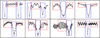 |
Fig. 3 Same as Fig. 2 but for observational light curve images as exported from DETOCS. |
| In the text | |
|
Fig. 4 All pulsation (red) and minimum (blue) ground truth bounding boxes in one image area. (See text for details.) |
| In the text | |
|
Fig. 5 Loss and mAP variation for the SSD model during training and evaluation. The black and red lines refer to training and validation values, respectively. The blue dashed line corresponds to the 6200th epoch, the step for the final model. The plot data was smoothed exponentially by a factor of 0.6 to emphasise the trend. The TensorBoard parameter plots are available in the provided Google Colab notebook8. |
| In the text | |
|
Fig. 6 Samples of different detection performances on observational light curve images in the validation set with a predicted bounding box for each ground truth annotation for the SSD model. Detected patterns (in red and blue bounding boxes) with the maximum (left, TIC 73672504) and minimum (right, TIC 232637376) average IoU values are compared to ground truth annotations (green dashed boxes). The numbers above the boxes correspond to the IoU value for the related detection. The letters P and M refer to pulsation and minimum patterns, respectively. |
| In the text | |
|
Fig. 7 Confusion matrices for the overall (left) and only the observational (right) data in the validation dataset calculated based on the predicted class and bounding boxes by setting the IoU and confidence level to 0.5. We note that 0.08% of pulsation and 0.41% of the minimum patterns were detected as background, namely, predicted as though they are not objects of interest for the overall data, while the percentages are 0.36% and 0.26% for observations. The letters P and M refer to pulsation and minimum patterns, respectively. |
| In the text | |
|
Fig. 8 Precision-recall curves of the detection in IoU=0.5 (left), IoU=0.75 (middle), and IoU=0.9 (right) thresholds. The black and red lines correspond to minimum and pulsation patterns, respectively. The calculations were conducted by using the code given by Padilla et al. (2021). |
| In the text | |
|
Fig. 9 Variation of loss and mAP across epochs for the Faster R-CNN model. The black and red lines represent training and validation values, respectively, while the blue dashed line indicates the epoch corresponding to the final model. The TensorBoard parameter plots are available in the accompanying Google Colab notebook8. |
| In the text | |
|
Fig. 10 Examples of varying detection performance of the Faster R-CNN model on observational light curve images from the validation set displaying predicted bounding boxes for each ground truth annotation. The detected patterns (in red and blue bounding boxes) with the highest (left, TIC 158794976) and lowest (right, TIC 232637376) average IoU values are compared against ground truth annotations (green dashed boxes). The numbers above each box indicate the IoU value for the corresponding detection. The letters P and M denote pulsation and minimum patterns, respectively. The yellow box on the right panel represents the additional detection that is not present in the ground truth annotations. |
| In the text | |
|
Fig. 11 Confusion matrices for the overall data (left) and observational data only (right) in the validation dataset calculated using predicted class and bounding boxes, with the IoU and confidence threshold set to 0.5 with the Faster R-CNN model. The letters P and M denote pulsation and minimum patterns, respectively. |
| In the text | |
|
Fig. 12 Precision-recall curves for the Faster R-CNN model at IoU thresholds of 0.5 (left), 0.75 (middle), and 0.9 (right). The black and red lines represent the minimum and pulsation patterns, respectively. |
| In the text | |
|
Fig. 13 Plot showing the loss and mAP as they change with increasing epochs for the YOLO model. The black and red lines represent training and validation values, respectively, and the blue dashed line marks the epoch of the final model. The TensorBoard parameter plots are available in the provided Google Colab notebook8. |
| In the text | |
|
Fig. 14 Different detection performances on observational light curve images from the validation set showing predicted bounding boxes for each ground truth annotation using the YOLO model. The detected patterns, enclosed in red and blue boxes, with the highest (TIC 354922610, left) and lowest (TIC 323292655, right) average IoU values are compared to the ground truth annotations marked by green dashed boxes. The numbers above each box indicate the IoU value for that detection. The letters P and M represent pulsation and minimum patterns, respectively. |
| In the text | |
|
Fig. 15 Confusion matrices for the overall data (left) and observational data (right) in the validation dataset derived based on predicted classes and bounding boxes using the YOLO model, with IoU and confidence threshold set at 0.5. The letters P and M stand for pulsation and minimum patterns. |
| In the text | |
|
Fig. 16 Precision-recall curves of the YOLO model illustrated for IoU thresholds of 0.5 (left), 0.75 (middle), and 0.9 (right). The minimum patterns are indicated by the black line, while pulsation patterns are indicated by the red line. |
| In the text | |
|
Fig. 17 The decrement in Loss and mAP with increasing epochs for the EfficientDet D1 model is illustrated. The black and red lines denote training and validation values, respectively. The blue dashed line marks the final model at the 7100th epoch. TensorBoard parameter plots are available in the provided Google Colab notebook8. |
| In the text | |
|
Fig. 18 Examples of detection performance variation of the EfficientDet D1 model on observational light curve images from the validation set, featuring predicted bounding boxes for each ground truth annotation. Detected patterns, highlighted in red and blue boxes, with the highest (left, TIC 350030939) and lowest (right, TIC 355151781) average IoU values are compared to the ground truth annotations shown in green dashed boxes. The numbers above the boxes represent the IoU values for each detection. The letters P and M stand for pulsation and minimum patterns, respectively. |
| In the text | |
|
Fig. 19 Confusion matrices for the overall dataset (left) and only the observational data (right) in the validation set. The matrices were generated based on predicted classes and bounding boxes using the EfficientDet D1 model and by setting an IoU and confidence threshold of 0.5. We consider that 0.1% and 0.6% of the minimum patterns are misclassified as pulsation for the overall (left) and observational data (right), respectively. The letters P and M denote pulsation and minimum patterns. |
| In the text | |
|
Fig. 20 Precision-recall curves for the EfficientDet D1 model at IoU thresholds of 0.5 (left), 0.75 (middle), and 0.9 (right). The black line corresponds to minimum patterns and the red line to pulsation patterns. |
| In the text | |
|
Fig. 21 Learning curves for the non-pretrained CNN model. Left: variation of loss over epochs. Right: accuracy of the box predictor as training progresses. The black and red lines represent training and validation values, respectively, with the blue dashed line marking the epoch of the final model. |
| In the text | |
|
Fig. 22 Samples of detection performance on observational light curve images from the validation set displaying predicted bounding boxes for each ground truth annotation for the non-pretrained CNN model. The detected patterns, shown in red and blue boxes, with the highest (left, TIC 298734307) and lowest (right, TIC 409934330) average IoU values are compared to the ground truth annotations, marked by green dashed boxes. The numbers above each box represent the IoU value for the respective detection. The letters P and M denote the pulsation and minimum patterns, respectively. |
| In the text | |
|
Fig. 23 Confusion matrices for the overall data (left) and the observational data (right) in the validation set. The matrices were computed based on predicted classes and bounding boxes, with the IoU and confidence thresholds set to 0.5 and using the non-pretrained CNN-based model. We note that the model is considerably unsuccessful at detecting patterns, especially on observational data. The letters P and M denote pulsation and minimum patterns, respectively. |
| In the text | |
|
Fig. 24 Precision-recall curves for the non-pretrained CNN model plotted with IoU thresholds of 0.5 (left), 0.75 (middle), and 0.9 (right). The black line denotes the minimum, and the red line indicates pulsation patterns. We note that the recall axis is shortened in the rightmost plot for better visibility. |
| In the text | |
|
Fig. 25 Detection performance of Faster-RCNN (a1, a2), YOLO (b1, b2), EfficientDet D1 (c1,c2), and non-pretrained CNN-based (d1, d2) models on the light curves in Fig. 6. |
| In the text | |
|
Fig. 26 Histogram showing the distribution of average IoU values achieved in detecting patterns on the observational light curves in which both classes (P and M) are detected. The numbers in the box brackets refer to the value intervals. The term ‘Eff’ stands for EfficientDet D1 model. |
| In the text | |
|
Fig. C.1 Same as Fig. 25 but for the detection performance of SSD (a1, a2), YOLO (b1, b2), EfficientDet D1 (c1,c2) and non-pretrain CNN-based (d1, d2) models on the light curves in Fig. 10. |
| In the text | |
|
Fig. C.2 Same as Fig. 25 but for the detection performance of SSD (a1, a2), Faster-RCNN (b1, b2), EfficientDet D1 (c1,c2) and non-pretrain CNN-based (d1, d2) models on the light curves in Fig. 14. |
| In the text | |
|
Fig. C.3 Same as Fig. 25 but for the detection performance of SSD (a1, a2), Faster-RCNN (b1, b2), YOLO (c1,c2) and non-pretrain CNN-based (d1, d2) models on the light curves in Fig. 18. |
| In the text | |
|
Fig. C.4 Same as Fig. 25 but for the detection performance of SSD (a1, a2), Faster-RCNN (b1, b2), YOLO (c1,c2) and EfficientDet D1 (d1, d2) models on the light curves in Fig. 22. |
| In the text | |
|
Fig. C.5 Mosaic of 36 detections with the highest average confidence scores on short cadence Kepler data of 40 targets using the SSD model. The values above the red and blue bounding boxes refer to the confidence of pulsation (P) and minimum (M) patterns. |
| In the text | |
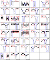 |
Fig. C.6 Same as Fig. C.5, but for 38 detection using Faster R-CNN model. |
| In the text | |
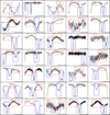 |
Fig. C.7 Same as Fig. C.5, but for 35 detection using YOLO model. |
| In the text | |
|
Fig. C.8 Same as Fig. C.5 but for the light curves of the systems having the highest 25 confidence scores of pulsation patterns. Be aware that the inference results are contaminated by large scatterings in maximum phases of some light curves. See text for details. |
| In the text | |
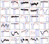 |
Fig. C.9 Same as Fig. C.6 but for the 30 systems in Kepler Eclipsing Binaries catalogue. |
| In the text | |
Current usage metrics show cumulative count of Article Views (full-text article views including HTML views, PDF and ePub downloads, according to the available data) and Abstracts Views on Vision4Press platform.
Data correspond to usage on the plateform after 2015. The current usage metrics is available 48-96 hours after online publication and is updated daily on week days.
Initial download of the metrics may take a while.