| Issue |
A&A
Volume 695, March 2025
|
|
|---|---|---|
| Article Number | A245 | |
| Number of page(s) | 26 | |
| Section | Cosmology (including clusters of galaxies) | |
| DOI | https://doi.org/10.1051/0004-6361/202451768 | |
| Published online | 25 March 2025 | |
QUIJOTE scientific results
XVIII. New constraints on the polarisation of the anomalous microwave emission in bright Galactic regions: ρ Ophiuchi, Perseus, and W43
1
Instituto de Astrofísica de Canarias, E-38200 La Laguna, Tenerife, Spain
2
Departamento de Astrofísica, Universidad de La Laguna, E-38206 La Laguna, Tenerife, Spain
3
Imperial College London, Blackett Lab, Prince Consort Road, London SW7 2AZ, UK
4
Institut d’Astrophysique de Paris, UMR 7095, CNRS & Sorbonne Université, 98 bis boulevard Arago, 75014 Paris, France
5
Laboratoire de Physique Subatomique et de Cosmologie, Université Grenoble Alpes, CNRS/IN2P3, 53 Avenue des Martyrs, Grenoble, France
6
Consejo Superior de Investigaciones Científicas, E-28006 Madrid, Spain
7
Universidad de Cantabria, Departamento de Ingeniería de Comunicaciones, Edificio Ingenieria de Telecomunicación, Plaza de la Ciencia 1, 39005 Santander, Spain
8
Astrophysics Group, Cavendish Laboratory, University of Cambridge, J J Thomson Avenue, Cambridge CB3 0HE, UK
9
Kavli Institute for Cosmology, University of Cambridge, Madingley Road, Cambridge CB3 0HA, UK
10
Instituto de Física de Cantabria (IFCA), CSIC-Univ. de Cantabria, Avda. los Castros, s/n, E-39005 Santander, Spain
11
Departamento de Física Moderna, Universidad de Cantabria, Avda. de los Castros s/n, 39005 Santander, Spain
12
CNRS-UCB International Research Laboratory, Centre Pierre Binétruy, IRL2007, CPB-IN2P3, Berkeley, CA 94720, USA
13
Jodrell Bank Centre for Astrophysics, Alan Turing Building, Department of Physics & Astronomy, School of Natural Sciences, The University of Manchester, Oxford Road, Manchester M13 9PL, UK
14
Departamento de Física, Facultad de Ciencias, Universidad de Córdoba, Campus de Rabanales, Edif. C2. Planta Baja., E-14071 Córdoba, Spain
15
Department of Physics, Xi’an Jiaotong-Liverpool University, 111 Ren’ai Road, Suzhou Dushu Lake Science and Education Innovation District, Suzhou Industrial Park, Suzhou 215123, PR China
⋆ Corresponding authors; This email address is being protected from spambots. You need JavaScript enabled to view it.
, This email address is being protected from spambots. You need JavaScript enabled to view it.
Received:
2
August
2024
Accepted:
29
January
2025
Abstract
This work focuses on the study of the anomalous microwave emission (AME), an important emission mechanism between 10 and 60 GHz whose polarisation properties are not yet fully understood and is therefore a potential contaminant for future cosmic microwave background (CMB) polarisation observations. We used new QUIJOTE-MFI maps at 11, 13, 17, and 19 GHz obtained from the combination of the public wide survey data and additional 1800 h of dedicated raster scan observations together with other public ancillary data, including WMAP and Planck, to study the polarisation properties of the AME in three Galactic regions: ρ Ophiuchi, Perseus, and W43. We obtained the spectral energy distributions (SEDs) of the three regions over the frequency range 0.4–3000 GHz in intensity and polarisation. The intensity SEDs are well described by a combination of free-free emission, thermal dust, AME, and CMB anisotropies. In polarisation, we extracted the flux densities using all available data between 11 and 353 GHz. We implemented an improved intensity-to-polarisation leakage correction that allowed reliable polarisation constraints well below the 1% level from Planck-LFI data to be derived for the first time. A frequency stacking of maps in the range 10–60 GHz allowed us to reduce the statistical noise and to push the upper limits on the AME polarisation level. We obtained upper limits on the AME polarisation fraction of the order ≲1% (95% confidence level) for the three regions. In particular, we obtained ΠAME < 1.0% (at 28.4 GHz), ΠAME < 0.9% (at 28.4 GHz), and ΠAME < 0.28% (at 33 GHz) in ρ Ophiuchi, Perseus, and W43, respectively. At the QUIJOTE 17 GHz frequency band, we found ΠAME < 5.0% for ρ Ophiuchi, ΠAME < 3.4% for Perseus, and ΠAME < 0.85% for W43. We note that for the ρ Ophiuchi molecular cloud, the new QUIJOTE-MFI data allowed us to set the first constraints on the AME polarisation in the range 10–20 GHz. Our final upper limits derived using the stacking procedure are ΠAME < 0.58% for ρ Ophiuchi, ΠAME < 0.67% for Perseus, and ΠAME < 0.31% for W43. Altogether, these are the most stringent constraints to date on the AME polarisation fraction of these three star-forming regions.
Key words: ISM: general / HII regions / cosmic background radiation / cosmology: observations / diffuse radiation / inflation
© The Authors 2025
 Open Access article, published by EDP Sciences, under the terms of the Creative Commons Attribution License (https://creativecommons.org/licenses/by/4.0), which permits unrestricted use, distribution, and reproduction in any medium, provided the original work is properly cited.
This article is published in open access under the Subscribe to Open model. This email address is being protected from spambots. You need JavaScript enabled to view it. to support open access publication.
1. Introduction
Characterisation of the polarised Galactic foregrounds (Ichiki 2014) in the microwave and sub-millimetre ranges is fundamental to the search for the inflationary B-mode anisotropy in the cosmic microwave background (CMB) polarisation (Kamionkowski et al. 1997; Zaldarriaga & Seljak 1997). This B-mode signal, generated by inflationary gravitational waves, is contaminated by Galactic foregrounds. An accurate modelling of these foregrounds is very important to producing clean CMB maps suitable for their cosmological exploitation, both in intensity and in polarisation. Synchrotron and thermal dust emissions are known to be strongly polarised. The former is generated by cosmic rays spiralling in the Galactic magnetic field and is known to have polarisation fractions of up to ∼40% (Kogut et al. 2007). The latter originates in the Galactic interstellar dust and has polarisation fractions of up to ∼20% in some regions of the sky (Planck Collaboration XIX 2015; Planck Collaboration X 2016; Planck Collaboration XXV 2016). The free-free emission from thermal bremsstrahlung is known to have practically zero polarisation. While the mechanisms responsible for synchrotron, thermal dust, and free-free emissions are physically well understood, there is a fourth important Galactic foreground, referred to as ‘anomalous microwave emission’ (AME), whose nature and polarisation properties are still under debate. The first evidence of Galactic AME was achieved almost 30 years ago as a dust-correlated signal at frequencies 10–60 GHz that could not be explained in terms of other physical mechanisms (Kogut et al. 1996; Leitch et al. 1997). Neither free-free nor synchrotron were able to explain its observed properties. Its spectrum, characterised by a bump peaking at ∼20 − 30 GHz and being notably different from those of free-free and synchrotron emissions, has suggested a scenario with a fresh new component emission important through the 10-60 GHz frequency range (de Oliveira-Costa et al. 1999; Watson et al. 2005; Hildebrandt et al. 2007).
Over the past years, significant efforts have been dedicated to improving the observational characterisation of AME in intensity and in polarisation, with the goal being to shed light on theoretical models. Observations of large sky areas (de Oliveira-Costa et al. 1998, 1999; Davies et al. 2006; Kogut et al. 2007; Todorović et al. 2010; Macellari et al. 2011; Planck Collaboration XXV 2016; Rennie et al. 2022; Fernández-Torreiro et al. 2023); of individual Galactic clouds, (Watson et al. 2005; Casassus et al. 2006; Dickinson et al. 2009; AMI Consortium 2009; Tibbs et al. 2010; Vidal et al. 2011; Planck Collaboration XX 2011; Planck Collaboration XV 2014; Poidevin et al. 2023), deriving constraints in some cases on the AME polarisation degree (Battistelli et al. 2006; Dickinson et al. 2006; Casassus et al. 2007, 2008; Mason et al. 2009; Génova-Santos et al. 2011, 2015, 2017; Battistelli et al. 2015; Poidevin et al. 2019; Herman et al. 2023); and of extra-galactic objects (Murphy et al. 2010; Scaife et al. 2010; Peel et al. 2011; Planck Collaboration XV 2014; Hensley et al. 2015; Murphy et al. 2018; Tibbs et al. 2018; Battistelli et al. 2019; Linden et al. 2020; Bianchi et al. 2022; Fernández-Torreiro et al. 2024) have contributed to the understanding of the physical properties of this emission. Determining if the AME presents any polarisation level is of vital importance for missions searching for the faint B-mode signal (Ade et al. 2019; Abazajian et al. 2022; LiteBIRD Collaboration 2023). As demonstrated by Remazeilles et al. (2016), neglecting an AME component with a polarisation fraction as low as ∼1% could potentially lead to a non-negligible bias on the measured tensor-to-scalar ratio.
Different models and theories have been proposed to explain the origin of AME. Probably the most accredited model is the electric dipole emission (EDE) from small fast-spinning dust grains in the interstellar medium (ISM; Draine & Lazarian 1998a,b; Ali-Haïmoud et al. 2009; Hoang et al. 2010; Ysard et al. 2011; Silsbee et al. 2011; Ali-Haïmoud 2013; Hoang et al. 2013; Ysard et al. 2022). There are two main hypotheses regarding the exact composition of these dust grains. The first suggests that polycyclic aromatic hydrocarbons (PAHs) could be responsible for the signal excess (Draine & Lazarian 1998a,b). This argument is made on the basis of the correlation between AME and mid-infrared dust emission in PAH-dominated bands at 8–12 μm (Ysard et al. 2010). The second theory suggests that generic very small grains (VSGs) could generate this emission (Hensley et al. 2016; Hensley & Draine 2017). Unfortunately, the exact shape of the spinning dust spectra depends on a large number of parameters that are not sufficiently well constrained observationally, thus complicating the confirmation of any of the models by observation (Ali-Haïmoud et al. 2009; Ysard et al. 2011; Ali-Haïmoud 2013).
A different model known as magnetic dipole emission (MDE) has also been proposed. In this case, a magnetic field produces the alignment of the grains so they emit radiation when their minimum energy state is reached. Differently from spinning dust, MDE is a mechanism of thermal emission (Draine & Lazarian 1999; Draine & Hensley 2013). One further alternative model is based on thermal emission from amorphous dust grains, and it is also able to reproduce the AME microwave bump in total intensity (Jones 2009; Nashimoto et al. 2020). Measuring the level of polarisation of AME may give very useful information on theoretical models. It has been proposed that quantum-mechanical effects may suppress grain alignment, leading to very low polarisation levels if the AME is produced by an EDE mechanism (Draine & Hensley 2016). However, most models of MDE (Draine & Lazarian 1999; Draine & Hensley 2013; Hoang & Lazarian 2016) predict polarisation levels above the current upper limits that are at a level of ≲1% (López-Caraballo et al. 2011; Dickinson et al. 2011; Rubiño-Martín et al. 2012a; Génova-Santos et al. 2017). Nevertheless, Draine & Lazarian (1999) also proposed a model with random inclusions of metallic Fe that produces very low polarisation (< 1%). For a more detailed and complete review on models and the observational status of AME, we refer to Dickinson et al. (2018).
In this paper we present a detailed analysis, in intensity and in polarisation, of the AME in three of the brightest and best-studied Galactic regions: the ρ Ophiuchi and Perseus molecular clouds and the W43 molecular complex. Notably, ρ Ophiuchi and Perseus are ideal sources for the study of AME because they are located in regions with relatively low Galactic emission and because they have a very low level of free-free emission, therefore enabling a clean separation of the AME component. On the other hand, W43 has significant free-free emission, but it is among the Galactic regions harbouring more AME.
The main novelty of this work is the study of these three regions with a new and more sensitive dataset at frequencies sensitive to AME. We used new maps of QUIJOTE-MFI at 10–20 GHz obtained through a combination of wide-survey data covering the full northern sky (Rubiño-Martín et al. 2023) and deeper and more sensitive observations of these sources. The paper is organised as follows. Section 2 presents a brief description of the physical properties of the three studied regions. Section 3 describes the dataset used to build the intensity spectral energy distributions (SEDs) and to derive the polarisation constraints. Section 4 describes the methodology used, including the aperture photometry technique to extract flux densities and the component separation via modelling of the derived SEDs using a Markov chain Monte Carlo (MCMC) technique. We also describe in this section the colour-correction methodology, the correction of the intensity-to-polarisation leakage in Planck-LFI, and a frequency-stacking technique aimed at improving the AME polarisation constraints. Section 5 presents our main results obtained on ρ Ophiuchi, Perseus, and W43. The main conclusions of this work are presented in Sect. 6.
2. The Galactic regions ρ Ophiuchi, Perseus, and W43
In this section we present a brief description of the physical properties of the three Galactic regions that are the focus of this work: the ρ Ophiuchi and Perseus molecular clouds and the W43 molecular complex. The left panel of Fig. 1 shows the location on the sky of these three sources, superimposed on the QUIJOTE 11 GHz wide survey map. Their central coordinates, that have been taken from the SIMBAD database1, are listed in Table 1. Figure 2 displays high angular-resolution maps of Planck-HFI 857 GHz showing the different substructures of these regions.
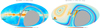 |
Fig. 1. Left: QUIJOTE-MFI wide survey intensity map at 11 GHz (Rubiño-Martín et al. 2023) with the locations of the three regions studied in this paper overlaid. Right: Map of the number of hits (per pixel of HEALPixNside = 512 and in units of seconds) for horn 3 11 GHz after combination of the wide survey data in nominal mode with the raster scan data listed in Table B.2. |
Basic characteristics of the sources studied in this paper.
2.1. ρ Ophiuchi molecular cloud
ρ Ophiuchi is a molecular cloud in the Gould Belt located around ∼1° south of the ρ Ophiuchi star, with an angular size ≈5°. At a distance of D = 144 ± 7 pc (Zucker et al. 2019) it is the closest star-forming region to Earth. It is undergoing intermediate star formation, concentrated in three clouds of dense gas and dust: the Lynds dark clouds L 1688, that contains the Ophiuchus star cluster and is considered the main cloud of this complex (Abergel et al. 1996), L 1689 and L 1709 (see Fig. 2). Ultra-violet radiation from the hottest young stars in this cluster dissociates the surrounding gas. The best example is the prominent photodissociation region (PDR) ρ Oph-W which is excited by the star B2V HD147889 and constitutes the western edge of L1688 (Liseau et al. 1999; Habart et al. 2003). This is the region where the bulk of the AME is produced. This was first identified by Casassus et al. (2008) as an excess of emission at 31 GHz using data from the CBI interferometer. AME in this region was subsequently studied by Dickinson et al. (2011), who derived upper limits on its polarisation fraction of the order of ≲1%, and by Planck Collaboration XX (2011). More recently, Arce-Tord et al. (2020) discovered spatial variations on the spinning dust emissivity using observations of the CBI2 interferometer, while Casassus et al. (2021) used observations with ATCA, at a finer angular resolution, to study the AME in this region at smaller scales.
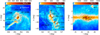 |
Fig. 2. High-angular resolution maps from Planck-HFI 857 GHz around the positions of the three studied regions. In the case of the ρ Ophiuchi and Perseus molecular clouds we indicate the positions of different compact clouds extracted from different catalogues and the location of the main ionising star. In W43 we indicate the positions of the molecular clouds identified in the CO survey of Solomon et al. (1987), highlighting in red the two most massive ones. The solid circle delineates the aperture used for flux density integration and the dashed circles enclose the ring used for background subtraction (see Sect. 4.1). |
2.2. Perseus molecular cloud
The Perseus molecular cloud complex is a relatively nearby giant molecular cloud at a distance of 294 ± 15 pc (Zucker et al. 2019). The full cloud is around 30 pc across (∼6° ×3° on the sky) and encompasses six dense cores: B 5, IC 348, B 1, NGC 1333, L 1455 and L 1448 (see Fig. 2). Anomalous microwave emission originates mainly around the dust shell G159.6-18.5 located southwest of IC348, that is illuminated by the O9.5-B0V star HD278942, and filled by an HII region (Andersson et al. 2000). Anomalous microwave emission from G159.6-18.5 was first detected by Watson et al. (2005) using data from the COSMOSOMAS experiment, a result that is widely recognised as the first unambiguous detection of AME in a compact region. This region dominated most of the dust-correlated signal first identified by de Oliveira-Costa et al. (1999) via correlations between data at 10 GHz and 15 GHz from the Tenerife experiment and dust maps. Using high-angular resolution data at 33 GHz with the VSA interferometer, Tibbs et al. (2010) concluded that the bulk of the AME is diffuse (originated in scales larger than 10 arcmin, that is the angular resolution of the VSA). Battistelli et al. (2006) analysed 11 GHz data in polarisation from the COSMOSOMAS experiment and found a tentative signal with a polarisation fraction of  , whereas López-Caraballo et al. (2011) and Dickinson et al. (2011) determined upper limits of ≲1% (95% C.L.) on the AME polarisation fraction using WMAP 23 GHz data2. More recently, Génova-Santos et al. (2015) presented new flux densities and polarisation upper limits using QUIJOTE MFI commissioning data with a shallower sensitivity than those used in this paper. Planck Collaboration XXV (2016) applied a different analysis consisting of looking for correlations between a weighted polarised intensity map constructed from the combination of WMAP and Planck data and the AME intensity map from Commander, on a larger region around the Perseus molecular cloud, to derive an upper limit of < 1.6%.
2.3. W43 molecular complex
W43 (source number 43 of the catalogue of Westerhout 1958) is one of the richest molecular complexes and with one of the highest star formation rates in our Galaxy (Nguyen Luong et al. 2011). It is located at a distance of ≈5.5 kpc and has a physical size of ∼140 pc, extending almost 2° along the direction of Galactic longitude. According to Nguyen Luong et al. (2011) this complex includes more than 20 molecular clouds with high velocity dispersion (Solomon et al. 1987) and is surrounded by atomic gas that extends up to ∼290 pc. In Fig. 2 we show the locations of these compact molecular clouds, highlighting (red circles) the positions of W43-main and W43-south that are the most massive ones (Nguyen Luong et al. 2011). The core of W43-main harbours a well-known giant HII region powered by a particularly luminous cluster of Wolf-Rayet and OB stars (Blum et al. 1999). AME in W43 was first identified by Irfan et al. (2015). Using new data from QUIJOTE MFI, Génova-Santos et al. (2017) determined an upper limit on the AME polarisation fraction of < 0.22% that, as of today, is the most stringent constraint on the polarisation of the AME. These results are revisited in this paper.
3. Data
We used twenty five total-intensity maps between 0.408 GHz and 3000 GHz to build the SEDs of the three regions, and sixteen maps in polarisation. In Table B.1 we list the main properties of these maps. Although we indicate the parent angular resolution of these maps, all of them have been smoothed to an effective angular resolution of 1°. They all use a HEALPix3 (Górski et al. 2005) pixelisation with resolution Nside = 512. Details of each of these surveys are given in the following subsections.
3.1. QUIJOTE data
The new data presented in this paper were acquired with the QUIJOTE experiment, (Rubiño-Martín et al. 2012b). One of the science drivers of this experiment is to characterise the polarisation of the low-frequency foregrounds, mainly the synchrotron and the AME. QUIJOTE is located at the Teide Observatory (Tenerife, Spain) at 2400 m above the sea level and at geographical longitude 16° 30′38″ West and latitude 28° 18′04″ North. Observing at the minimum elevation attainable by QUIJOTE of 30° at this latitude allows one to reach declinations as low as −32°. QUIJOTE consists of two telescopes with an offset crossed-Dragone optics design, with projected apertures of 2.25 m for the primary and 1.89 m for the secondary mirror, providing highly symmetric beams (ellipticity < 0.02) with very low sidelobes (≤40 dB) and polarisation leakage (≤25 dB). This combination of optics and mount was chosen to allow the telescope to spin fast at a constant elevation while observing. The two telescopes are equipped with three instruments covering the frequency range 10 − 40 GHz. The first instrument on the first QUIJOTE telescope, the so-called multi-frequency instrument (MFI), consisted of four horns, each of which observed in two frequency bands: horns 1 and 3 observed at 11 and 13 GHz, while horns 2 and 4 observed at 17 and 19 GHz; each had a 2 GHz bandwidth. The full width at half maximum (FWHM) is ≈55 arcmin at 11 and 13 GHz, and ≈39 arcmin at 17 and 19 GHz. The data used in this paper were taken with this instrument.
3.1.1. New raster scan observations
The QUIJOTE-MFI instrument observed between 2012 and 2018. Most of the time during this period (more than 9000 hours) was dedicated to observations in the so-called “nominal mode” (continuous rotation of the telescope at constant elevation), leading to maps covering the full northern sky (total sky fraction of ≈73%) and with sensitivities of ∼60 − 200 μK deg−1 in intensity and ∼35 − 40 μK deg−1 in polarisation. These “wide survey” maps were publicly released in January 2023 and their properties are described in detail in Rubiño-Martín et al. (2023). This paper uses a combination of these data in the nominal mode with deeper observations in raster scan mode, leading to higher sensitivities at the positions of these regions.
The QUIJOTE-MFI raster scan observations consisted of back-and-forth constant-elevation scans of the telescope performed with an effective scanning speed on the sky of 1 deg/s (the telescope is moved with angular velocity around the azimuth axis ωAZ = 1/cos(EL) deg/s). Each observation was typically comprised of a few hundred scans4 (total duration per observation of ∼1 hour), in such a way that rotation of the sky leads to a map size along the elevation direction similar to the scan length along the azimuth direction. Typically, between one and five observations were performed every day, and were repeated in consecutive days with a civil time offset of 4 minutes (same sidereal time). Table B.2 presents a summary of the observations in raster scan mode that are used in this paper, including total integration times. Leaving aside the observations in the nominal mode leading to the wide survey maps, these fields, and particularly HAZE and PERSEUS, are among the fields with the highest total observing time of QUIJOTE-MFI. The final maps of ρ Ophiuchi combine observations in this field with wider observations in the fields HAZE and HAZE2 intended to investigate the excess of microwave emission around the Galactic Centre that has been addressed in Guidi et al. (2023). The HAZE and HAZE2 observations are clearly reflected in the map of number of hits of Fig. 1 as a redder wide region south of the ρ Ophiuchi field. The redder region to the northeast of W43 corresponds to the HAZE3 field, it has not been included in Table B.2 because it does not overlap with either of the three regions that we study in this paper. The ρ Ophiuchi maps used in this paper are the same as in Guidi et al. (2023).
We have performed three different types of observations around the Perseus molecular cloud, as indicated in Table B.2. The so-called PERSEUS field consists of azimuth scans of size 15°. This value is close to the minimum scan size in QUIJOTE-MFI observations so that the source is observed by the four horns in a single observation. In order to maximise the integration time per unit solid angle, and therefore to improve the map sensitivity, in this case we also performed the observations called PERSEUS-H2 and PERSEUS-H3 that are respectively centred in horns 2 and 3 and use a smaller scan length of 5° and 6° respectively. Given the smaller map size, in these cases the source is only seen by horn 2 in PERSEUS-H2 and by horn 3 in PERSEUS-H3. This observing strategy leads to much higher integration time per unit solid angle (see values in Table B.2). We note that these are a different set of observations from those used in Génova-Santos et al. (2015) that were performed between December 2012 and April 2013 during the commissioning of QUIJOTE-MFI. In the final Perseus maps presented here, we discarded those observations because at that time, the internal calibration signal that is now used by default to monitor and correct gain variations (see Sect. 2.2.1 of Rubiño-Martín et al. 2023) was not available.
The observations in raster scan mode in W43 were described in Génova-Santos et al. (2017). In this paper we use these same observations, but with improved data processing (see Sect. 3.1.2), in combination with the wide survey data presented in Rubiño-Martín et al. (2023). These latter data have an average integration time per solid angle of 0.16 h deg−2 (see Table B.3) and then will not have a significant impact on the final map sensitivities. However, they help reduce various systematic effects, and in particular, the combination of more scanning directions contributes to a more efficient destriping procedure and to minimise the large-scale systematic effects in polarisation.
3.1.2. Data reduction
The QUIJOTE-MFI data processing pipeline is introduced in Sect. 2.2 of Rubiño-Martín et al. (2023) and will be explained in depth in a dedicated paper (Génova-Santos et al. in prep.). The QUIJOTE-MFI maps on which the analyses presented in this paper are based were generated following the same procedure. Briefly: (i) the global gain calibration is based on regular raster scan observations of two bright radio sources, Tau A and Cas A; (ii) the same observations of Tau A are used to calibrate the polarisation direction of the detectors; (iii) gain variations in long time scales are corrected using an internal calibration signal that is emitted by a thermally stabilised diode every 30 seconds; (iv) projection of the TOD data onto maps is done using a destriping algorithm called PICASSO (Guidi et al. 2021) that is an adaptation of the MADAM approach (Keihänen et al. 2005) to QUIJOTE data.
The previous study of QUIJOTE-MFI on the Perseus molecular cloud (Génova-Santos et al. 2015), apart from being based on a different and less sensitive dataset (map sensitivities were a factor ∼5 worse, depending on the frequency and horn), did not implement points (iii) and (iv), i.e. no gain correction was executed and the map making was based on a simpler median filter, that results in a less efficient removal of intensity 1/f noise and suppression of the angular scales larger than the filter size. The previous QUIJOTE-MFI study in W43 (Génova-Santos et al. 2017) used the same raster scan data of this paper (but without the combination with the data in the nominal mode), as it was mentioned in the previous subsection. In that case, the same destriping algorithm as in this paper was used. However, the gain correction of point (iii), that is an important improvement in the current analysis, was not applied. Another important difference with respect to those previous studies concerns the global gain calibration. In both Génova-Santos et al. (2015) and Génova-Santos et al. (2017) it was based on the Tau A and Cas A models presented in Weiland et al. (2011). The maps used in this paper are calibrated instead using an improved model for Tau A that will be described in detail in Génova-Santos & Rubiño-Martín (in preparation; the model is given in Eq. (9) of Rubiño-Martín et al. 2023). The uncertainty of these models in the QUIJOTE-MFI frequency range is of the order of 5%, that is considered to be the global calibration uncertainty of the QUIJOTE maps. In addition, we have developed an improved and more-reliable method, based on a beam fitting algorithm, to extract from QUIJOTE-MFI data the reference flux density of Tau A that is used to calibrate the maps. These modifications lead to differences of the order of 5–10% in the final flux densities of the sources. Given the improvements commented before on gain correction and calibration, the results presented in this paper should be deemed more reliable.
3.1.3. Maps
Maps at each of the four QUIJOTE-MFI frequencies are produced from the calibrated time-ordered data using the destriping algorithm described in Sect. 3.1.2. The map-making parameters (baseline length and priors on the correlated-noise parameters) are the same as those adopted for the wide-survey maps (see Table 5 in Rubiño-Martín et al. 2023). Data affected by different systematic effects (radio interference, strong gain variations, etc) are flagged following the methodology and criteria explained in Sect. 2.2.2 of Rubiño-Martín et al. (2023). The post-processing of the maps (weights for the combination of channels and the filtering with the function of the declination, as described respectively in Sects. 2.4.1 and 2.4.2 of Rubiño-Martín et al. 2023) is also identical to the one used for the wide-survey maps. Table B.3 lists the effective integration times per unit solid angle used to generate the maps, calculated in a region around the central coordinates of each source indicated in Table 1, except for W43 for which we used coordinates l = 35.8°, b = −0.02° to avoid the nearby masked region affected by contamination from geostationary satellites (see Sect. 2.2.2 of Rubiño-Martín et al. 2023). Comparison of these numbers with the total observed times shown in Table B.2 gives an idea of the fraction of flagged data in each case (we note that the total integration times given in Table B.2 are for horn 3). The region most affected by flagging is Perseus, owing to significant contamination from radio interference in many of the observations. On the other hand ρ Ophiuchi is the region least affected, and in this case we kept 64% of the data at 11 GHz. In all cases, the amount of flagging is larger in polarisation than in intensity. Table B.3 also shows a comparison of the integration times in the nominal mode and in the combination of nominal plus raster scan data, highlighting the notably higher integration times achieved in the raster scans. This fact becomes also evident in the map of the number of hits illustrated in the right panel of Fig. 1, which clearly shows a higher integration time in the regions where these three sources are located.
The maps at 11 and 13 GHz were generated using only data from horn 3. As with other QUIJOTE-MFI papers, maps from horn 1 are not used due to having important systematic effects, in particular problems with the positioning of the polar modulator (Rubiño-Martín et al. 2023). At 17 and 19 GHz the maps of ρ Ophiuchi and Perseus from horns 2 and 4 are combined through a weighted mean that uses predefined constant weights (see Sect. 3 of Rubiño-Martín et al. 2023). In the case of the W43 field, we use only maps from horn 2, as in this case the polarisation maps of horn 4 seem to be affected by intensity-to-polarisation leakage. Prior to that combination, intensity and polarisation maps produced from the correlated and uncorrelated channels are also combined. In the case of polarisation, uncorrelated channels are only used for data taken under a configuration such that the two channel outputs have correlated 1/f noise properties. All these details, as well as the definition of correlated and un-correlated channels, are explained in depth in Rubiño-Martín et al. (2023). The noise of the lower and upper frequency bands of each horn are significantly correlated (up to 80% in intensity) because of the use of the same low-noise amplifiers, as explained in Sect. 4.3.3 of Rubiño-Martín et al. (2023). Ideally, the noise covariance between the 11 and 13 GHz maps on the one hand and between the 17 and 19 GHz maps on the other should be taken into account. However, we have verified that this has no significant impact on the results derived in this paper (differences of 3% in the worst case on the derived model parameters), so for the sake of simplicity we have ignored this covariance term.
Final QUIJOTE-MFI intensity (Stokes I) and polarisation (Stokes Q and U) maps at their native angular resolution are shown in Figs. 3, 4, and 5, for ρ Ophiuchi, Perseus and W43, respectively. For comparison, we show also the WMAP 23 GHz and Planck 30 GHz maps. In total intensity these maps are clearly dominated by emission from each of these sources, and the increase of flux density from 11 to 19 GHz associated with the AME is evident even by eye. Thanks to the presence of an adjacent HII region (its position is indicated in the figure through a solid circle), that is dominated by free-free emission, the region showing the clearest visual evidence of AME is ρ Ophiuchi. Here the photodissociation region that harbours the AME, located towards the centre of the map, becomes more and more intense relative to the free-free emission in the HII region as the frequency increases. Meanwhile, the polarisation maps are mostly consistent with noise. The exceptions are: (i) the diffuse signal shown at 11 and 13 GHz in the ρ Ophiuchi maps which is due to one of the diffuse bright filaments (Vidal et al. 2015) originating from the Galactic centre (see Sect. 5.1), and that leaves a temperature gradient running from the northeast to the southwest, and (ii) diffuse emission seen in the Q map of W43 distributed along the Galactic plane which is most-likely due to diffuse Galactic synchrotron emission as already discussed in Génova-Santos et al. (2017). The origin of this emission is discussed in depth in Sect. 5.3, while in Appendix A we present a detailed study of the possible contribution of instrumental effects to this signal.
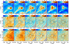 |
Fig. 3. Intensity and polarisation maps around the ρ Ophiuchi molecular cloud from QUIJOTE-MFI and from the two lowest-frequency bands of WMAP and Planck. The three rows show respectively I, Q and U maps, while the columns correspond to 11, 13, 17 (Horn 2), 19 (Horn 2), 23 and 30 GHz from left to right. The solid circle shows the aperture we used for flux integration, whereas the two dashed circles enclose the ring we used for background subtraction. The small circle inside the background annulus towards the west indicates the mask applied to avoid a strong HII source. The grey areas towards the southwest at 17 and 19 GHz are masked due to satellite contamination. For the sake of better visualisation, these maps are shown at their raw angular resolution, although all the analyses presented in this paper have been performed on maps convolved to a common angular resolution of 1°. |
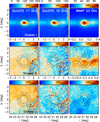 |
Fig. 5. Intensity and polarisation maps around the W43 molecular cloud. The three rows show, respectively, I, Q, and U maps, while the columns correspond to QUIJOTE-MFI 17 (Horn 2) and 19 GHz (Horn 2) and to WMAP 23 GHz, from left to right. The solid circle shows the aperture we used for flux integration, whereas the two dashed circles enclose the ring we used for background subtraction. |
The noise properties of these maps are evaluated from jack-knife maps resulting from the subtraction of the two half-mission maps (see Sect. 4.1 of Rubiño-Martín et al. 2023). The noise levels in intensity and in polarisation derived from these maps, in units of standard deviations in μK in a region with a solid angle of 1 deg2, are listed in Table B.3. It becomes obvious from this table that cancellation of 1/f noise in polarisation leads to noise levels at these angular scales a factor ∼3 better than in intensity. The scale dependence of intensity 1/f noise, and residual 1/f noise in polarisation, can be appreciated in Fig. 15 of Rubiño-Martín et al. (2023), which shows that it starts to impact at scales larger than ∼1° and gradually increases at larger angular scales as usual. While in our analyses we use maps resulting from the combination of horns 2 and 4, as explained above, in Table B.3 we have quoted noise figures from these two horns independently. There is a clear improvement over the noise levels achieved in the wide survey data (nominal mode), that are of the order 30 − 80 μK deg−1 in polarisation (see Table 14 of Rubiño-Martín et al. 2023). At 11 and 13 GHz we achieve noise levels in polarisation of ∼7 − 10 μ K deg−1 in Perseus and in ρ Ophiuchi. Together with the maps obtained around the Taurus molecular cloud (see Table 1 of Poidevin et al. 2019) and on M31 (see Table 2 of Fernández-Torreiro et al. 2024) these are among the deepest and most sensitive observations obtained with QUIJOTE-MFI. Instantaneous sensitivities (sensitivity in an integration of one second) per channel can be estimated from the values of Table B.3 as  , where σmap is the map sensitivity listed in the last three columns, tint is the integration time per unit solid angle listed under the ‘n+r’ columns, and the factor
  must be applied only when the maps use a combination of correlated and uncorrelated channels, so that we get the sensitivity to the measurement of I, Q or U through only one of these two combinations. This calculation gives values of the order of 0.6 − 1.0 mK s1/2 in Q and U and of the order of 3 − 5 mK s1/2 in I, that are consistent with the typical values derived in other regions (see e.g. Table 13 of Rubiño-Martín et al. 2023).
3.2. Ancillary data
3.2.1. Low-frequency radio surveys
Data in total intensity at frequencies below QUIJOTE-MFI are needed to model the free-free emission5. At these frequencies we used the surveys listed in Table B.1: (i) the full-sky “Haslam” map at 0.408 GHz (Haslam et al. 1982), (ii) the “Dwingeloo” 0.820 GHz map of the northern sky (Berkhuijsen 1972), (iii) the “Reich” map of the northern sky at 1.42 GHz (Reich & Reich 1986), (iv) the S-PASS survey of the southern sky at 2.3 GHz (Carretti et al. 2019) and (v) the “HartRAO” map of the southern sky at 2.326 GHz (Jonas et al. 1998). For the Haslam, Reich and HartRAO maps we used the public versions of Platania et al. (2003). The data from the Dwingeloo survey have been extracted from the MPIfR’s Survey Sampler6 and projected into a HEALPix pixelisation. The S-PASS maps were downloaded from the LAMBDA database7. As we do for all other surveys, these maps are convolved to a common angular resolution of 1°, except the Dwingeloo map whose native angular resolution is 1.2°. The slightly larger angular resolution of this map may have an impact on the derived results that is accounted for in the 10% calibration uncertainty that is assigned to this map (see Table B.1).
Except for the Haslam map, all these surveys have a partial sky coverage. The Dwingeloo map does not cover the ρ Ophiuchi region, while neither the S-PASS nor the HartRAO surveys cover the Perseus region. For ρ Ophiuchi and W43, the flux densities of these two last surveys were averaged into one single measurement at 2.3 GHz. For W43 we also used the C-BASS (Jones et al. 2018) flux densities extracted by Irfan et al. (2015) appropriately rescaled in intensity, as explained in Génova-Santos et al. (2017). The calibration of both the Reich and the HartRAO maps is referenced to the full-beam solid angle. To overcome this issue, and translate the calibration to the main-beam, we multiply the Reich map by 1.55 (Reich & Reich 1988). In the case of the HartRAO map, for ρ Ophiuchi and Perseus we have applied the standard factor of 1.45 derived by Jonas et al. (1998), while in W43 we have applied a smaller factor of 1.2 to account for the fact that its angular size is larger than the telescope’s beam (see related discussion in Génova-Santos et al. 2017). Uncertainties on these factors are accounted for in the 10% calibration uncertainties assigned to these maps (see Table B.1). Other systematic effects that affect these maps are uncertainties related to the determination of zero levels, but our analyses are insensitive to this thanks to the subtraction of an average background level through our aperture photometry technique (see Sect. 4.1).
3.2.2. Microwave, millimetre and sub-millimetre surveys: WMAP, Planck, and DIRBE
In the microwave regime, we used data from WMAP and Planck, that helped us better constrain the AME spectrum. In the millimetre and sub-millimetre ranges, we used (in addition to Planck) data from COBE-DIRBE that allowed us to model the spectrum of the thermal dust emission.
The WMAP satellite produced full-sky maps, in intensity and polarisation, at 23, 33, 41, 61 and 94 GHz (Bennett et al. 2013). In this analysis we use the version of WMAP 9-year maps smoothed to a resolution of 1° which are available from the LAMBDA database8. The Planck mission (Planck Collaboration I 2020) produced full-sky maps at central frequencies of 28, 44, 70, 100, 143, 217, 353, 545 and 857 GHz in total intensity, and in polarisation in the seven lower-frequency bands. We have used intensity maps from the Planck 2018 data release (PR3). The 100, 217 and 353 GHz frequency maps have been corrected from CO emission using the Type 1 CO maps. We note that there is a negligible difference between using PR2, PR3 or PR4 to extract flux densities of compact sources in total intensity (see e.g. Poidevin et al. 2023). In polarisation we have used PR3 for LFI and PR4 for HFI. In the LFI we have applied our own implementation of the leakage correction in polarisation, for which we have used the projection maps that are only available for PR3 (see Sect. 4.4.2). At the HFI frequencies the PR4 data have better systematics in polarisation (Planck Collaboration LVII 2020). When comparing polarised flux densities derived from PR3 and PR4 we have found larger differences (beyond the measurement uncertainty) at 100 GHz, and found that the PR3 values deviate clearly from the spectral trend established by measurements at other frequencies, contrary to PR4. These Planck maps have been downloaded from the Planck Legacy Archive (PLA)9.
The spectral coverage of DIRBE, an infrared instrument onboard the COBE satellite, spans from 1.25 to 240 μm (Hauser et al. 1998). We have used maps at 240 μm (1249 GHz), 140 μm (2141 GHz) and 100 μm (2997 GHz), which are the three frequencies dominated by the population of big grains that can be modelled with a single modified blackbody spectrum. We have used the zodiacal-light subtracted mission average (ZSMA) maps regridded into the HEALPix format.
Table B.1 lists the calibration uncertainties ascribed to each of these surveys that have been used in the subsequent analyses. They are the same used in previous recent works by the QUIJOTE collaboration (see e.g. Poidevin et al. (2023) and references therein).
4. Methodology
4.1. Flux-density estimation through aperture photometry
Intensity and polarisation flux densities are calculated through a standard aperture photometry method applied on the 1°-smoothed maps of each region. This is a well-known and widely used technique (López-Caraballo et al. 2011; Planck Collaboration XX 2011; Génova-Santos et al. 2015, 2017; Poidevin et al. 2019; López-Caraballo et al. 2024) consisting of integrating temperatures of all pixels within a given aperture, and subtracting a background level estimated through the median of all pixels in an external ring. The flux density is then given by
 (1)
(1)
where
 (2)
(2)
is the conversion factor between thermodynamic differential temperature (KCMB units) and flux-density (units of 1026 Jy), Ti is the thermodynamic temperature of pixel i inside the aperture, n1 is the number of pixels in the aperture,  is the median temperature of all pixels in the background region, Ωpix is the solid angle corresponding to one pixel and x = hν/(kBTCMB) is the dimensionless frequency.
We have considered two different methods to estimate the error of Sν. The first one is based on the analytical propagation of pixel errors through the equation
![Mathematical equation: $$ \begin{aligned} \sigma _{\rm stat}({S_\nu }) = a(\nu )\, \sigma (T) \left[ \frac{1}{n_{1}} + \frac{\pi }{2} \frac{1}{n_{2}} \right]^{1/2} ~~, \end{aligned} $$](/articles/aa/full_html/2025/03/aa51768-24/aa51768-24-eq7.gif) (3)
(3)
where σ(T) is the error of the temperature value of each pixel that is considered uniform and is derived from the pixel-to-pixel standard deviation calculated in the background ring, and n2 is the total number of pixels in the background annulus. This equation assumes perfectly uncorrelated noise between pixels. As explained in Sect. 3.1.3, in general the noise is spatially correlated due to the presence of 1/f residuals. In addition background fluctuations on scales larger than the pixel size also introduce correlated noise. The noise correlation function could be introduced in Eq. (3), but its determination is not trivial. Alternatively, as a second method that accounts jointly for both contributions (1/f and white noise), we derive flux densities in ten apertures located around the source, using the same aperture and external annulus radii, and derive σstat(Sν) through the scatter of these estimates. We have applied this method to estimate uncertainties in the polarisation flux density estimates. In total intensity we have used this same method in ρ Ophiuchi and Perseus. In W43 we found out that uncertainties using Eq. (3) lead to a global fit with reduced χ2 close to one so in this case we decided to stick to this method. Details related with the calculation of the flux-density errors of each region are explained in the corresponding sections.
The calibration uncertainty of each survey is combined with the statistical error to derive a final global error as
 (4)
(4)
where δ is the calibration fractional error (quoted in Table B.1 in percent units).
Central coordinates and sizes of the circular aperture and of the inner and outer circles of the background ring are given in Table 1. In general we have opted to choose the same values as in previous studies of the same regions to allow for a more reliable comparison with previous results. For ρ Ophiuchi we have used the same parameters as in Planck Collaboration XX (2011) and in Dickinson et al. (2011). In this case, to obtain a more realistic background estimate we have removed the emission from the nearby HII region, which is brighter at QUIJOTE-MFI frequencies, by masking all pixels lying in a circle of radius 0.4° around the position (l, b) = (351.5°, 17.05°). In the case of Perseus we used the same configuration as in the intensity analysis of Génova-Santos et al. (2015), while for W43 we used that of Génova-Santos et al. (2017). Intensity flux densities for the three regions are shown in Table B.410, while flux densities calculated on Q and U maps are shown in Tables B.5, B.6 and B.7.
4.2. Spectral energy distribution modelling in total intensity
We modelled four different components in our frequency range, between 0.4 and 3000 GHz: free-free, AME, thermal dust and CMB anisotropies. The low-frequency spectra of the three molecular cloud complexes studied in this paper are fully dominated by free-free emission, and therefore the synchrotron emission is not considered in the fits. The physical models used for each of these components are briefly explained in the following subsection.
4.2.1. Sky model
4.2.1.1. Free-free emission.
Taking into account that Te(1 − e−τff) is the brightness temperature of the free-free emission for a medium with optical depth τff and electron temperature Te, the corresponding flux density can be calculated as
 (5)
(5)
Here, we considered the equations derived by Draine (2011) for the optical depth,
 (6)
(6)
and for the Gaunt factor,
![Mathematical equation: $$ \begin{aligned} g_{\rm ff} (\nu ) = \mathrm{ln}\left(\mathrm{exp} \left( 5.960 - \frac{\sqrt{3}}{\pi } \cdot \mathrm{ln} \left[\left(\frac{\nu }{\mathrm{GHz}}\right) \left(\frac{T_{\rm e}}{10^{4} \mathrm{K}}\right)^{-3/2} \right] \right) + e\right). \end{aligned} $$](/articles/aa/full_html/2025/03/aa51768-24/aa51768-24-eq11.gif) (7)
(7)
For the electron temperature we have used Te = 8000 K (same value as Planck Collaboration XX 2011 and Génova-Santos et al. 2015) for ρ Ophiuchi and Perseus and Te = 6038 K for W43; this last value is the same used in (Génova-Santos et al. 2017) and is extracted from a template of the free-free emission at 1.4 GHz produced by Alves et al. (2012) using radio recombination line data from the HI Parkes All-Sky Survey (HIPASS). The only remaining free parameter associated with the free-free component is the emission measure EM (units of pc ⋅ cm−6).
4.2.1.2. Thermal dust.
Following the common practise in the field (see e.g. Planck Collaboration XI 2014), the thermal dust emission was modelled as a single-component modified black-body (MBB) curve, νβdBν(ν, Td), that we normalised using the optical depth at 250 μm (1.2 THz), τ250:
 (8)
(8)
where the dust temperature Td and the emissivity index βd, together with τ250, are the three free parameters.
4.2.1.3. Anomalous microwave emission
Here, we modelled the AME through a phenomenological model consisting of a parabola in the log(S) – log(ν) plane (Stevenson 2014):
![Mathematical equation: $$ \begin{aligned} S_{\nu }^\mathrm{AME} (A_{\rm AME}, \nu _{\rm AME}, W_{\rm AME}) = {A_{\rm AME}} \cdot \mathrm{exp} \left[ -\frac{1}{2 {W_{\rm AME}}^2} \mathrm{ln}^2 \left(\frac{\nu }{\nu _{\rm AME}}\right) \right] , \end{aligned} $$](/articles/aa/full_html/2025/03/aa51768-24/aa51768-24-eq13.gif) (9)
(9)
where AAME is the maximum flux density, νAME the correspondent frequency for that maximum, and WAME the width of the parabola on the log-log plane. This phenomenological model reproduces with high fidelity the spinning dust models and, thanks to its simplicity and due to the difficulty of jointly fitting the large number of parameters of those models, is frequently used by other recent studies (Cepeda-Arroita et al. 2021; Poidevin et al. 2023; Fernández-Torreiro et al. 2023).
4.2.1.4. Cosmic microwave background
Although the CMB monopole (constant) term was cancelled in the background subtraction in our photometry method (see Sect.4.1), CMB fluctuations could still have a contribution in the angular scale of the aperture. They were then modelled as
 (10)
(10)
where the fitted parameter is the amplitude ΔTCMB.
4.2.2. Model selection
As described in the previous subsections our model consists of 8 free parameters: EM for the free-free emission, AAME, νAME and WAME for the AME, τ250, βd, and Td for the thermal dust emission and ΔTCMB for the CMB anisotropies. To sample the parameter posterior distributions we used the MCMC sampler from the EMCEE package (Foreman-Mackey et al. 2013). Table 2 shows the priors that we have placed on each parameter. Due to the CMB anisotropies being a subdominant component ΔTCMB is usually hard to constrain. Imperfections on the MBB model in the range ∼100 − 600 GHz could in some cases be absorbed by this component (Fernández-Torreiro et al. 2023). For this reason, in this case we chose to use Gaussian priors centred at zero. The width of this Gaussian prior has been fixed from the standard deviation of the flux-density estimates extracted on ∼300 random positions on a CMB map, using the aperture photometry configuration shown in Table 1. We use the CMB map extracted from Planck data using the SMICA component-separation algorithm. For the other parameters we have used top-hat priors. While for ρ Ophiuchi and Perseus we have used EM > 0 pc⋅cm−6, in the case of W43 we used a more stringent prior on the emission measure, 1000 < EM < 1500 pc⋅cm−6, that is driven by the information based on the radio recombination line data of Alves et al. (2012) (see related discussion in Génova-Santos et al. 2017). The final best-fit parameters are determined from the median values of the parameter posteriors, while their uncertainties are derived from the half difference of the 16 and 84 percentiles. In those cases where the distributions are quite asymmetric we have reported two different values for the negative and positive uncertainties. In Fig. 6 we represent the probability density functions, in two and one dimensions, and best-fit parameters and their uncertainties, for the best-fit model of W43. It is important to point out that, without QUIJOTE, the width of the fit of the AME is biased towards large values, and the peak frequency towards lower values, highlighting the importance of QUIJOTE in constraining the parameters of the AME.
Priors on the model parameters used in the fitting procedure.
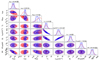 |
Fig. 6. Example of a corner plot of the two-dimension parameter space explored by the MCMC implemented in the EMCEE package corresponding to the W43 molecular complex. Blue and red contours correspond respectively to the fits with and without QUIJOTE data (see derived best-fit parameters in Table 3). Also shown are one-dimension marginalised posterior distributions from which the best-fit parameters and uncertainties are determined. |
Best-fitting model parameters for ρ Ophiuchi, Perseus, and W43 in intensity.
4.3. Colour correction
We have applied colour corrections for all surveys except for the low-frequency ones (0.408 to 2.326 GHz) where they are assumed to be unnecessary thanks to their narrower bandpasses (typically Δν/ν < 2%). Each flux density is multiplied by a colour-correction coefficient derived using the FASTCC code (Peel et al. 2022). For frequencies below and above 100 GHz we used two different approaches as described in Sect. 3.3.2 of Fernández-Torreiro et al. (2023). Briefly, for ν < 100 GHz we assumed a power-law model and the colour-correction coefficient was calculated from the fitted spectral index at each frequency, while for ν > 100 GHz the βd and Td fitted parameters of the MBB law are used to interpolate on a previously computed 2D grid. Colour corrections depend on the fitted model so the process is applied iteratively until convergence is reached. Colour corrections are typically ≲2% for QUIJOTE, WMAP and Planck-LFI, and ≲10% for Planck-HFI and DIRBE, that have considerably larger bandwidths.
4.4. Polarisation analyses
Flux densities in polarisation were calculated for frequencies between 11 GHz and 353 GHz. In this section we describe specific tools that are applied to the analysis of polarisation data.
4.4.1. Noise debiasing of the polarised intensity
Due to the polarised intensity  being a positive-defined quantity, noise in the measurement of Q and U lead to a positive bias on the measured values of P and of Π = P/I, that is more pronounced in the low signal-to-noise regime as it is our case. In this case knowledge of the full probability function of P (which is no longer Gaussian even if errors of Q and U are Gaussian distributed) is needed in order to reliably determine the most-likely values and confidence intervals of P and Π. We follow the same prescription that was described and applied in Rubiño-Martín et al. (2012a) and previous QUIJOTE papers (e.g. Génova-Santos et al. 2015, 2017). Specifically, to debias P we followed a Bayesian approach consisting of integrating the analytical posterior probability density function (PDF) given in Vaillancourt (2006). For Π we also integrate its PDF which, in this case, is evaluated through a Monte Carlo approach. In both cases we report best-fit values and 68% errors determined from these PDFs when the signal-to-noise ratio of the measured quantity is larger than
  . Otherwise, we quote upper limits at the 95% confidence level.
4.4.2. Correction of intensity-to-polarisation leakage in Planck LFI
One of the most important systematic effects in polarisation of Planck-LFI is intensity-to-polarisation leakage caused by the bandpass mismatch of the two orthogonally polarised arms of the same radiometer (see e.g. Planck Collaboration III 2016). Correction of this spurious signal requires knowledge of (i) the spectrum of the emission in intensity, (ii) the bandpasses of the two arms of the radiometer, and (iii) the scanning directions of each pixel to transform between sky and local coordinates. The way this correction is implemented is described in Sects. 11.1 to 11.4 of Planck Collaboration II (2016). The corrected Stokes parameters are given by Eq. (C.1) of Planck Collaboration XXVI (2016):
 (11)
(11)
where Qcorr and Ucorr are the corrected maps, Q and U are the raw maps, PQ and PU are the leakage projection maps (see Sect. 11.4 of Planck Collaboration II 2016), α is the spectral index of the sky emission (in flux-density units) in the considered frequency band and αCMB is the spectral index of the CMB (1.96, 1.90 and 1.75 at 28.4, 44.1 and 70.4 GHz respectively). For PR2 and PR3 the leakage-correction maps at an angular resolution of 1° and Nside = 256 obtained through this method are available in the PLA, while for PR4 this correction has already been applied in the public polarisation maps. In these public data products, the spectral index α has been obtained from the Commander algorithm (see Sect. 11.2 of Planck Collaboration II 2016) at an effective angular resolution of 1°. Instead of using those public maps, here we choose to implement our own correction using the more precise spectral index α derived from our fit to the intensity SED described in Sect. 4.2. To this aim, we downloaded from the PLA the PR3 projecting AQ and AU maps for each radiometer, and we built a projection map for each frequency band as (see Sect. 11.4 of Planck Collaboration II 2016)
![Mathematical equation: $$ \begin{aligned} P_{Q[U]} = \sum _k a_k A_{k,Q[U]}~~, \end{aligned} $$](/articles/aa/full_html/2025/03/aa51768-24/aa51768-24-eq36.gif) (12)
(12)
where the sum extends over all radiometers in each frequency and ak is the bandpass-mismatch a-factor for radiometer k given in Table 7 of Planck Collaboration II (2020).
Uncertainties in this procedure have been carefully accounted for and conservatively propagated to the final error bar. We have considered the uncertainties in the estimation of the ak factors quoted in Table 7 of Planck Collaboration II (2020) as well as uncertainties in the determination of the spectral index α that is introduced in Eq. (11). To this end, using Eq. (12) we generated PQ and PU maps using the ak values corresponding to the two extremes of the error bar, namely, ak − σ(ak) and ak + σ(ak), and plugged them into Eq. (11) to produce corrected maps. Similarly, we generated correction maps using spectral indices α − σα and α + σα. In both cases, we calculated Q and U flux densities in both sets of maps and defined two systematic uncertainties, respectively for ak and for α, as the difference between the two extreme values. These two systematic uncertainties are added in quadrature as two additional terms in Eq. (4).
To showcase the reliability of this procedure, in Fig. 7 we show the PR3 un-corrected maps, our PR3 corrected maps and the public PR4 corrected maps at 22.8 GHz and around W43. While the un-corrected maps show significant spurious emission in Q and U at the position of the source, with polarisation fraction of ∼1.5%, this is largely suppressed in the corrected maps. It is also clear that the PR4 maps still show some residual leakage emission, in particular in U, that is corrected with better accuracy in our implementation, likely thanks to a better reconstruction of the intensity spectral index that is introduced in Eq. (11). Diffuse emission distributed along the Galactic plane still remains in Q. We also note that, as in the correction procedure, we used the spectral index α for W43, and the corrected maps are more reliable in pixels close to the central coordinates of W43 (inside the circle of Fig. 7). As we move away from the source, the true underlying spectral index may deviate from that of W43, leading to a less precise correction. In any case, the leakage correction is more critical right at the position of W43, where the emission in total intensity is strong. Away from this source, the emission in total intensity is much fainter, so the polarisation leakage is much smaller and may be embedded in the noise.
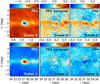 |
Fig. 7. Illustration of the effect of the polarisation leakage correction in Planck-LFI at 28.4 GHz around the position of W43. Stokes Q and U maps are represented respectively in the top and bottom panels. From left to right, the panels respectively show the PR3 raw (un-corrected) maps, the PR3 leakage-corrected maps using our own implementation (see Sect. 4.4.2 for details), and the public PR4 corrected maps. |
In Appendix A we present a detailed quantitative study of the level of leakage in Planck-LFI (as well as in WMAP), and we have showcased the reliability of the leakage-correction methodology which has been described in this section.
4.4.3. Improved polarisation constraints through frequency stacking
Previous similar studies have usually presented constraints on the polarisation fraction of AME at individual frequencies (López-Caraballo et al. 2011; Génova-Santos et al. 2015, 2017). Taking into account that the noise of data at different frequencies is statistically independent, here we consider combining the information at different frequency bands with the goal to improve the constraints on ΠAME = P/SAME. This combination can be done in different ways. One possibility would be to evaluate the PDF of ΠAME at each individual frequency and then combine them to derive a joint constraint on ΠAME, which is assumed here to be frequency-independent. We implemented this method and checked that it gives roughly consistent results with a different method based on a stacking at the map level that we used as a default. In this method, each pixel p of the stacked map is assigned a temperature value:
 (13)
(13)
where Tp, i is the temperature value, in KCMB units, of pixel p at frequency νi, νs = 22.8 GHz is the reference frequency at which the stacking is performed, η = x2ex/(ex − 1)2 is the conversion factor between thermodynamic differential temperature (KCMB units) and brightness Rayleigh-Jeans temperature (KRJ units) and wi is the weight corresponding to frequency νi. This stacking is performed independently for maps of Stokes I, Q and U, using the same weights. We note that stacking both Q and U independently assumes that an eventual AME polarisation component has a polarisation angle which is constant with frequency. This assumption could be circumvented by stacking directly on polarised intensity, but at the cost of introducing additional complications related with the noise bias discussed in Sect. 4.4.1.
We used optimal weights to minimise the final uncertainty on ΠAME which then accounts not only for the uncertainties on the I, Q and U flux densities but also for the AME amplitude at each frequency νi. In the presence of fully uncorrelated noise, these weights are given by
 (14)
(14)
In this equation IAME, i represents the AME flux density at frequency νi, calculated by subtracting from the measured flux density (calculated through Eq. (1) and listed in Table B.4) the flux densities of the sum of the rest of the components (free-free, CMB and thermal dust) resulting from our fitted model evaluated at the same frequency. The term in the denominator, σi, is the quadratic average of the errors of the flux-density estimates in Qi and Ui,  .
.
To account for the presence of noise correlations between frequency bands, that are due to 1/f residuals and to sky background fluctuations, we use the covariance matrix in the definition of the weights, that are then given by:
 (15)
(15)
where the sums run over frequencies, and the noise covariance matrix Ci, j is calculated using the flux-densities calculated on the random apertures at all frequencies (see Sect. 4.1). We calculate covariance matrices for Q and U independently and Ci, j is the arithmetic mean of the two. We find strong noise correlations, of around 50–70% for pairs of adjacent frequencies below 33 GHz, that are driven by the background fluctuations. For instance, in W43 we find a maximum correlation of 78% between WMAP and Planck lowest frequency bands.
For each region we have stacked the maps corresponding to the same frequencies for which we have quoted AME polarisation constraints in Tables B.5, B.6 and B.7. These maps have been convolved to a common angular resolution of 1° prior to the stacking. The final stacked maps are displayed in Fig. 8. No significant emission is visible in either the Q or U maps except for i) diffuse emission running southwest to northeast in the ρ Ophiuchi U map which is due to a large-scale synchrotron spur (see Sect. 3.1.3), ii) diffuse emission along the Galactic plane in the Q map of W43 (see Sect. 3.1.3), and iii) polarised emission originated in the supernova remnant (SNR) W44 which is visible towards the left of the Q and U maps of W43.
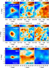 |
Fig. 8. Intensity and polarisation stacked I, Q, and U maps at a reference frequency of 22.8 GHz and at the position of the three sources studied in this paper. These maps are the result of a weighted average of maps at frequencies around the AME peak frequency convolved at a common angular resolution of 1° and were obtained following the procedure outlined in Sect. 4.4.3. |
Flux densities were calculated on these maps through aperture photometry using Eq. (1) with the reference frequency νs = 22.8 GHz. The residual AME flux density on the stacked map was calculated as
 (16)
(16)
where Ss is the flux density calculated on the stacked I map and the terms inside the parenthesis are the flux densities of the different modelled components evaluated at frequency νi. The stacked AME polarisation fraction is then calculated as  , where Qs and Us are flux densities calculated on the stacked maps, and debiased using the methodology outlined in Sect. 4.4.1.
5. Results and discussion
This section presents the main results of this paper: the modelling of the intensity SED of the three studied regions and the inferred polarisation constraints for both the AME and the thermal dust emission. Figures 9, 10, and 11 show the intensity SEDs and fitted models respectively for ρ Ophiuchi, Perseus and W43. In Table 3 we show the best-fit parameters for these three regions. To illustrate the effect of the inclusion of QUIJOTE-MFI data we also show the best-fit parameters when these data are excluded from the fit. Tables B.5, B.6 and B.7 show the corresponding polarisation constraints. In the following sections we discuss the main results for the three regions separately.
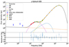 |
Fig. 9. ρ Ophiuchi intensity SED. QUIJOTE-MFI data points are depicted in red together with other ancillary data (blue), including WMAP 9-yr (green), Planck (orange), and COBE-DIRBE data (light green). At intermediate frequencies, the excess emission associated with the AME clearly shows up. A joint fit has been performed consisting of the following components: free-free (orange line), AME log-normal model (purple line), CMB (blue line), and thermal dust (green-olive line). The black line represents the sum of all components. |
5.1. ρ Ophiuchi
Figure 9 shows the SED of the ρ Ophiuchi molecular cloud. Although the AME in this region has been extensively studied in the past (Casassus et al. 2008; Planck Collaboration XX 2011), QUIJOTE-MFI data provides, for the first time, measurements of the AME spectrum below the WMAP lowest frequency of 22.8 GHz, as already shown in Poidevin et al. (2023). Evidence for the presence of AME in this region has been solidly established for a long time, as the lack of signal at low frequencies (we note that all estimated flux densities below 10 GHz are compatible with zero) is inconsistent with the flattening of the spectrum at frequencies below ∼60 GHz being due to free-free emission. We note that the three lower-frequency data points (that are depicted in Fig. 9 as upper limits at confidence level of 95%) were included in the fit using their central values and error bars. QUIJOTE-MFI data have allowed for the first time to delineate the downturn of the AME spectrum at low frequencies. This allows constraining of the AME parameters, especially νAME and WAME, with much better precision, as can be seen in Table 3. In this case, there is no improvement in the uncertainty of AAME after the inclusion of the QUIJOTE-MFI data because the SED is markedly flat between 20 and 40 GHz, so WMAP and Planck data in this range are sufficient to anchor the AME amplitude. The data allowed for the determination of the model parameters for nearly all components with high precision, except the value of EM, which is consistent with an upper limit owing to a lack of detected emission at low frequencies. These parameters are consistent with those derived in previous studies (Planck Collaboration XX 2011; Poidevin et al. 2023).
Table B.5 shows Q and U flux densities, together with constraints on the polarised flux density and on the polarisation fraction of the AME for frequencies below 44.1 GHz, and for the thermal dust emission for frequencies above 60.5 GHz. These are the first constraints on the AME polarisation fraction on this region at QUIJOTE-MFI and Planck frequencies. We note that we detected a positive signal in U at frequencies up to 22.8 GHz. As already commented by Dickinson et al. (2011), this signal is associated with a relatively bright synchrotron spur that runs diagonally across the maps. This creates a notable gradient running from southwest to northeast which is more apparent at 11 GHz and 13 GHz (see maps of Fig. 3). A fit of these U values to a power-law model yields a spectral index α = −1.1 ± 0.3, characteristic of synchrotron emission. The signal from this spur leads to Pdb values away from zero at some frequencies, degrading the upper limits on ΠAME shown in Table B.5. Yet the derived upper limit of ΠAME < 1.0% for Planck-LFI 28.4 GHz is the most stringent constraint on the AME polarisation on this region; for comparison, Dickinson et al. (2011) had obtained ΠAME < 1.4% at 22.8 GHz. The strongest constraint from QUIJOTE-MFI is ΠAME < 5.0% at 16.8 GHz. The combination of maps of different frequencies described in Sect. 4.4.3 allowed us in this case to significantly improve the constraint, giving ΠAME < 0.58%. This is the most stringent upper limit on the AME polarisation level ever achieved in this region. It is worth emphasising at this point that these constraints have been obtained on a region of ≈1 degree, and therefore a polarised signal in smaller angular scales, which may have been smeared out through integration of different polarisation directions in our aperture, cannot be excluded.
Table B.5 also gives values of the polarisation fraction of the thermal dust emission at frequencies between 60.5 GHz and 353 GHz. These values are compatible with a constant value of Πdust = (1.8 ± 0.2)%, with χred2 = 1.1, although the 100 GHz point deviates at 1.6σ from this value11. We remind that these values have been obtained on maps convolved at a common angular resolution of 1°. Visual inspection of the Planck-HFI maps at their parent angular resolution reveals inhomogeneity of the polarisation direction at angular scales below 1°, and hence we conclude that the fractional polarisation of the thermal dust emission is intrinsically higher at finer angular scales.
5.2. Perseus molecular cloud
Figure 10 shows the SED of the Perseus molecular cloud, together with the best-fit model whose parameters are given in Table 3. It becomes clear from this table that the inclusion of the QUIJOTE-MFI data in the fit enables a more precise modelling of all AME parameters. Flux densities, as well as the best-fit model, are consistent with those derived in previous studies (Watson et al. 2005; Planck Collaboration XX 2011; Génova-Santos et al. 2015; Poidevin et al. 2023) in spite of small differences resulting from differences in the data analysis. QUIJOTE-MFI data in this region had already been published before (Génova-Santos et al. 2015). There was also previous intensity data in the same frequency range coming from the COSMOSOMAS experiment (Watson et al. 2005). The main improvement of the data presented in this paper comes from the higher integration time per unit solid angle (see Sect. 3.1.1). Yet no clear polarisation signal is visible in the maps of Fig. 4 nor in the stacked maps displayed in Fig. 8.
Table B.6 shows Q and U flux densities, together with constraints on the polarised flux density and on the polarisation fraction of the AME for frequencies below 44.1 GHz, and for the thermal dust emission for frequencies above 60.5 GHz. As for the other two regions, errors are estimated in all cases through the scatter of the flux density values calculated on ten apertures around the source. In this particular case, the raster scan maps have a size of ≈6° (see Table B.2), and the random apertures fall in a region that, owing to not being covered by these observations, has a poorer sensitivity. To overcome this issue, we have rescaled the errors derived from the random apertures by the ratio of the pixel-to-pixel RMS calculated on the combined map (raster and nominal data) to the pixel-to-pixel RMS calculated on the map with nominal data only. Thanks to the more sensitive data, the new QUIJOTE-MFI upper limits are better by a factor ≈1.6 than those presented in Génova-Santos et al. (2015). The most stringent upper limits at an individual frequency come from WMAP 22.8 GHz and Planck-LFI 28.4 GHz and are similar to those obtained by López-Caraballo et al. (2011) using WMAP 7-year data.
The upper limit derived from the stacked maps, ΠAME < 0.67%, that notably improves the constraints obtained at any individual frequency. Table B.6 shows a polarisation fraction of the thermal dust emission in the Perseus molecular cloud of Πdust ≈ 7%. In this case, the Planck-HFI maps at their parent angular resolution do not show a noticeable variation of the polarisation direction, so this value may be representative of the typical level of polarisation in finer angular scales within this region.
5.3. W43 molecular complex
QUIJOTE-MFI maps at 16.8 and 18.8 GHz at the position of W43 are shown in Fig. 5. Owing to this region being located close to the equatorial plane, it is affected by radio-emission contamination from geostationary satellites (Fig. 1 shows that it is very close to the masked stripe). This has left some residual contamination which is seen towards the west of these maps. This contamination is more harmful at 11 and 13 GHz and then at these two frequencies it has only been possible to derive reliable flux densities in total intensity.
The WMAP 22.8 GHz map displayed in Fig. 5 exhibits clear diffuse emission in Q along the Galactic plane. In Génova-Santos et al. (2017) we had hypothesised that this emission could be residual free-free or AME polarisation originating in W43 or diffuse synchrotron emission from the Galactic plane. While the Planck data analysed in Génova-Santos et al. (2017) was affected by intensity-to-polarisation leakage, the improved leakage correction implemented in this paper (see Sect. 4.4.2) leads to a Q map with a similar structure to the WMAP 22.8 GHz. This Q signal has a polarisation degree of ≈0.3% at 22.8 GHz. The similarity of the WMAP and Planck-LFI maps at these two frequencies, and the behaviour of the flux densities in Q at higher frequencies showing a monotonic decrease (see Table B.7) could naturally lead to the conclusion that this is a real signal and that the leakage is controlled to levels of ∼0.2% or better. On the contrary, the signal in U shows a different behaviour, with variations in sign at a level larger than the uncertainty and with amplitude of ∼0.2%, pointing to the presence of possible leakage residuals or any other unaccounted systematic effects at this level. This also becomes evident in the comparison of the WMAP and Planck-LFI U maps shown in Figs. 5 and 7, which show different structures. We have performed a joint fit of the Q and U values to a power-law (common spectral index and different amplitudes in Q and U) that gives α = −1.47 ± 0.94, a spectral index that is consistent with synchrotron emission. However, this fit has χ2 = 35.4 with 15 degrees of freedom, tentatively pointing to an underestimation of the uncertainties. We have undertaken a detailed study on bright unpolarised sources which shows that the residual intensity-to-polarisation leakage in Planck-LFI is at a level below 0.2% (see Appendix A). This is precisely of the same order as the signals in Q and U in W43. Therefore, we believe that with the current data it is not possible to claim that the signal in Q is real, even if the frequency spectrum traced by three different experiments could be suggestive that there could be some contribution from diffuse synchrotron emission or even possibly from the AME originating in W43. Disentangling between these hypotheses would require data in the same frequency range but with a control of systematic effects below the 0.2% level. This is a goal for the QUIJOTE TFGI instrument operating at 30 and 40 GHz. Future polarisation data from C-BASS at 5 GHz in this region will also be very useful, in particular to test the synchrotron hypothesis.
Given the ambiguity on the interpretation of the origin of the Q signal in W43, we have decided to quote upper limits on the polarisation fraction of AME, as shown in Table B.7. We have obtained ΠAME < 0.28% at 33.0 GHz. This region gives the most stringent constraints on the level of AME polarisation ever achieved. In Génova-Santos et al. (2017) we had obtained ΠAME < 0.22% at 40.6 GHz. The reason why the constraint quoted in Table B.7 is looser is differences in the intensity modelling of AME that lead to a lower residual AME flux density at this frequency. The stacked maps displayed in Fig. 8 also show a positive signal in Q, and lead to a constraint of ΠAME < 0.31%.
In this case, the stacking procedure does not lead to a more stringent upper limit because it is affected by the positive Q signal which is measured at individual frequencies. In other words, the stacking reduces the uncertainty on the measurement of this positive signal, but the upper limit is not affected because it depends on the central value and not on its uncertainty. This leads us to the conclusion that any future improvement on the derived upper limits in this region depends more on a better understanding of the residual polarisation signals (potentially through data in a different frequency range) than on improving the sensitivity. Table B.7 also lists the polarisation degree of thermal dust emission at frequencies above 93.5 GHz, that has a value of Πdust ≈ 1%. In this case, inspection of the Planck-HFI maps at their parent angular resolution reveals a notable spatial variability of the polarisation direction inside the 1° circular aperture, and then the intrinsic polarisation fraction in compact regions inside this aperture may be higher.
6. Conclusions
We have presented a joint study of the microwave AME emission, with emphasis on polarisation properties, of three of the brightest or best characterised AME regions on the sky: the ρ Ophiuichi and Perseus molecular clouds and the W43 molecular complex. This study has focused on the use of new or improved data from the QUIJOTE-MFI instrument at 11, 13, 17, and 19 GHz, that crucially help in better tracing the low-frequency tail of the AME spectrum and add further constraints on the AME polarisation at these frequencies. With respect to previous QUIJOTE studies on Perseus (Génova-Santos et al. 2015) and on W43 (Génova-Santos et al. 2017), we included new data and implemented an improved calibration and data processing that allowed us to reach sensitivity levels in polarisation in the range 10 − 50 μK deg−1 in these regions, depending on the frequency. The Perseus field is among the ones with a higher integration time per unit area of all fields observed with QUIJOTE-MFI. The QUIJOTE-MFI data have provided, for the first time, the detection of emission from the ρ Ophiuchi molecular cloud below 20 GHz and hence have allowed the first unambiguous characterisation of the AME spectrum below its peak in this region. In this paper, we have also presented the first constraints on the level of AME polarisation after applying an improved intensity-to-polarisation leakage correction of Planck-LFI data. This correction is based on the implementation of a careful correction of the intensity-to-polarisation leakage of Planck-LFI data, that is one of the most harmful systematic effects of these data because, if left uncorrected, it renders the data useless for any reliable analysis, especially in bright regions such as W43. This correction critically depends on an accurate characterisation of the intensity spectrum of the source, and we demonstrated that we have achieved a more reliable local correction using Planck PR3 data than what has been implemented in the PR4 maps. One further novelty of this paper is the application of a combination of all frequency bands sensitive to AME with the goal of improving the final constraint on the AME polarisation under the assumption that data at different frequencies are statistically independent.
We fitted the AME intensity spectra using a three-parameter phenomenological model consisting of a parabola in the log-log plane, which for certain combinations of parameters allowed us to accurately reproduce typical spinning dust spectra. As anticipated, the inclusion of the QUIJOTE-MFI data at frequencies 10–20 GHz helped us better constrain the parameters of this model, in particular its peak frequency (νAME) and width (WAME), whose errors decreased by a factor of two to three. This improved characterisation of the AME intensity spectrum is critical to deriving more reliable constraints on the AME polarisation level. In ρ Ophiuchi, we determined ΠAME < 1.0% (95% C.L.) from Planck-LFI at 28.4 GHz, and it is the most stringent constraint on the AME polarisation level in this region, slightly improving previous results in the same region (Dickinson et al. 2011). The most stringent constraint from QUIJOTE-MFI in this case is ΠAME < 5.0% at 16.8 GHz, while stacking all frequencies between 11.1 and 44.1 GHz leads to ΠAME < 0.58%. This is the second-best constraint ever achieved on an individual region after W43. The new QUIJOTE-MFI data on Perseus allowed us to achieve ΠAME < 3.4% at 16.8 and 18.8 GHz, that represents an improvement of ≈35% with respect to the results presented in Génova-Santos et al. (2015). At other frequencies, the constraints in Perseus are similar or slightly better than those derived in previous publications (López-Caraballo et al. 2011; Dickinson et al. 2011), with a best constraint of ΠAME < 0.9% from Planck 28.4 GHz. The constraints derived from W43 are slightly looser than those presented in Génova-Santos et al. (2017) because differences in the calibration and data processing have led to lower AME residual flux densities in total intensity. Here, we obtained a best upper limit of ΠAME < 0.28% from WMAP 33.0 GHz. In Perseus and in W43, the frequency-stacking technique respectively leads to ΠAME < 0.67% and ΠAME < 0.31%. The reason why the stacking in W43 does not improve the constraints to the level expected if the scatter of the individual measurements was consistent with the estimated errors is that in both cases, this scatter is driven not by statistical errors in the data but by a detection of residual polarisation emission. Improving these constraints requires a better understanding of the nature of this emission. This could be achieved through more sensitive data at various frequencies and ideally with a finer angular resolution in order to enable a precise characterisation of their spectra. In the case of W43, given that the measured signal in Q is at a level of 0.2% with respect to the measured intensity, a control of the instrument systematics at this level would also be needed, something that is hard to achieve. We have pushed the current data to their limits, and therefore improving the AME polarisation constraints in W43 requires further technical and observational efforts.
The constraints on AME polarisation presented in this paper are among the most stringent achieved on compact regions. They benefit from very low or no free-free emission on the ρ Ophiuchi and Perseus molecular clouds, that are both located away from the Galactic plane. On the other hand, W43 has significant free-free emission whose level is nevertheless relatively well anchored by the low-frequency data. These results are important not only to provide information on different AME models but also to assess the extent AME could be a problem for the search of the B-mode signal in the CMB polarisation. It must be borne in mind, however, that we have analysed three regions with specific physical conditions, so the results cannot be easily generalised. Additional constraints on AME polarisation in large portions of the sky are therefore needed, especially in what concerns primordial B-mode studies. It must also be noted that these constraints have been obtained at an angular scale of 1°, so the beam depolarisation effects could play a role, together with the mixing of different magnetic-field orientations along the line of sight. This could explain the relatively low polarisation degrees of the thermal dust emission obtained in the three regions. In what concerns B-mode searches, this might be sufficient, as this signal shows up on large angular scales. However, in order to provide useful feedback on AME modelling, it would be important to derive constraints on the AME polarisation at finer angular scales in order to avoid beam-depolarisation effects.
We note that López-Caraballo et al. (2011) quoted polarisation upper limits with respect to the total measured intensity emission, while Dickinson et al. (2011) used the residual AME intensity emission, that is what we do in this work.
We define a scan as the movement of the telescope at a fixed elevation between two fixed azimuths, either westwards or eastwards.
As explained in Sect. 4.2 the three regions that are studied in this paper are fully dominated by free-free emission, and do not show evidence of any synchrotron emission.
In this Table, the 2.3 GHz value in the case of ρ Ophiuchi is the weighted average of the flux densities derived from S-PASS and HartRAO. In the case of W43 the value comes from HartRAO, as the S-PASS map does not cover this region.
We did notice a larger deviation using PR3 data, that we ascribe to systematics, possibly related with CO intensity-to-polarisation leakage that is alleviated in PR4.
The subtraction of the signals measured by the two radiometers measuring the two orthogonal polarisation contains some residual intensity signal when the two bandpasses have different spectral shapes.
Acknowledgments
We thank the staff of the Teide Observatory for invaluable assistance in the commissioning and operation of QUIJOTE. The QUIJOTE experiment is being developed by the Instituto de Astrofisica de Canarias (IAC), the Instituto de Fisica de Cantabria (IFCA), and the Universities of Cantabria, Manchester and Cambridge. Partial financial support was provided by the Spanish Ministry of Science and Innovation under the projects AYA2007-68058-C03-01, AYA2007-68058-C03-02, AYA2010-21766-C03-01, AYA2010-21766-C03-02, AYA2014-60438-P, ESP2015-70646-C2-1-R, AYA2017-84185-P, ESP2017-83921-C2-1-R, PGC2018-101814-B-I00, PID2019-110610RB-C21, PID2020-120514GB-I00, IACA13-3E-2336, IACA15-BE-3707, EQC2018-004918-P, PID2023-150398NB-I00 and PID2023-151567NB-I00, the Severo Ochoa Programs SEV-2015-0548 and CEX2019-000920-S, the Maria de Maeztu Program MDM-2017-0765, and by the Consolider-Ingenio project CSD2010-00064 (EPI: Exploring the Physics of Inflation). We acknowledge support from the ACIISI, Consejeria de Economia, Conocimiento y Empleo del Gobierno de Canarias and the European Regional Development Fund (ERDF) under grant with reference ProID2020010108, and Red de Investigación RED2022-134715-T funded by MCIN/AEI/10.13039/501100011033. This project has received funding from the European Union’s Horizon 2020 research and innovation program under grant agreement number 687312 (RADIOFOREGROUNDS), and the Horizon Europe research and innovation program under GA 101135036 (RadioForegroundsPlus). This research made use of computing time available on the high-performance computing systems at the IAC. We thankfully acknowledge the technical expertise and assistance provided by the Spanish Supercomputing Network (Red Española de Supercomputación), as well as the computer resources used: the Deimos/Diva Supercomputer, located at the IAC. This research used resources of the National Energy Research Scientific Computing Center, that is supported by the Office of Science of the U.S. Department of Energy under Contract No. DE-AC02-05CH11231. RGG acknowledges support from Italian Ministry of education, university and research. MFT acknowledges support from from the Agencia Estatal de Investigación (AEI) of the Ministerio de Ciencia, Innovación y Universidades (MCIU), from the European Social Fund (ESF) under grant with reference PRE-C-2018-0067 and from the French Programme d’investissements d’avenir through the Enigmass Labex. FP acknowledges support from the Spanish Ministerio de Ciencia, Innovación y Universidades (MICINN) under grant numbers PID2022-141915NB-C21. DT acknowledges financial support from the XJTLU Research Development Fund (RDF) grant with number RDF-22-02-068. CHM acknowledges financial support from the Spanish Ministry of Science and Innovation under project PID2021-126616NB-I00. This research has made use of the SIMBAD database, operated at CDS, Strasbourg, France (Wenger et al. 2000). Some of the presented results are based on observations obtained with Planck (http://www.esa.int/Planck), an ESA science mission with instruments and contributions directly funded by ESA Member States, NASA, and Canada. We acknowledge the use of the Legacy Archive for Microwave Background Data Analysis (LAMBDA). Support for LAMBDA is provided by the NASA Office of Space Science. Some of the results in this paper have been derived using the healpy and HEALPix packages (Górski et al. 2005; Zonca et al. 2019).We have also used scipy (Virtanen et al. 2020), emcee (Foreman-Mackey et al. 2013), numpy (Harris et al. 2020), matplotlib (Hunter 2007), corner (Foreman-Mackey 2016) and astropy (Astropy Collaboration 2013, 2018) PYTHON packages.
References
- Abazajian, K., Addison, G. E., Adshead, P., et al. 2022, ApJ, 926, 54 [CrossRef] [Google Scholar]
- Abergel, A., Bernard, J. P., Boulanger, F., et al. 1996, A&A, 315, L329 [NASA ADS] [Google Scholar]
- Ade, P., Aguirre, J., Ahmed, Z., et al. 2019, JCAP, 2019, 056 [Google Scholar]
- Ali-Haïmoud, Y. 2013, Adv. Astron., 2013, 462697 [NASA ADS] [Google Scholar]
- Ali-Haïmoud, Y., Hirata, C. M., & Dickinson, C. 2009, MNRAS, 395, 1055 [CrossRef] [Google Scholar]
- Alves, M. I. R., Davies, R. D., Dickinson, C., et al. 2012, MNRAS, 422, 2429 [NASA ADS] [CrossRef] [Google Scholar]
- AMI Consortium (Scaife, A. M. M., et al.) 2009, MNRAS, 400, 1394 [CrossRef] [Google Scholar]
- Anderson, M. C., Keohane, J. W., & Rudnick, L. 1995, ApJ, 441, 300 [NASA ADS] [Google Scholar]
- Andersson, B. G., Wannier, P. G., Moriarty-Schieven, G. H., & Bakker, E. J. 2000, AJ, 119, 1325 [Google Scholar]
- Arce-Tord, C., Vidal, M., Casassus, S., et al. 2020, MNRAS, 495, 3482 [NASA ADS] [CrossRef] [Google Scholar]
- Astropy Collaboration (Robitaille, T. P., et al.) 2013, A&A, 558, A33 [NASA ADS] [CrossRef] [EDP Sciences] [Google Scholar]
- Astropy Collaboration (Price-Whelan, A. M., et al.) 2018, AJ, 156, 123 [Google Scholar]
- Battistelli, E. S., Rebolo, R., Rubiño-Martín, J. A., et al. 2006, ApJ, 645, L141 [NASA ADS] [CrossRef] [Google Scholar]
- Battistelli, E. S., Carretti, E., Cruciani, A., et al. 2015, ApJ, 801, 111 [Google Scholar]
- Battistelli, E. S., Fatigoni, S., Murgia, M., et al. 2019, ApJ, 877, L31 [Google Scholar]
- Bennett, C. L., Larson, D., Weiland, J. L., et al. 2013, ApJS, 208, 20 [Google Scholar]
- Berkhuijsen, E. M. 1972, A&AS, 5, 263 [NASA ADS] [Google Scholar]
- Bianchi, S., Murgia, M., Melis, A., et al. 2022, A&A, 658, L8 [NASA ADS] [CrossRef] [EDP Sciences] [Google Scholar]
- Blum, R. D., Damineli, A., & Conti, P. S. 1999, AJ, 117, 1392 [NASA ADS] [CrossRef] [Google Scholar]
- Carretti, E., Haverkorn, M., Staveley-Smith, L., et al. 2019, MNRAS, 489, 2330 [Google Scholar]
- Casassus, S., Cabrera, G. F., Förster, F., et al. 2006, ApJ, 639, 951 [NASA ADS] [CrossRef] [Google Scholar]
- Casassus, S., Nyman, L. Å., Dickinson, C., & Pearson, T. J. 2007, MNRAS, 382, 1607 [NASA ADS] [CrossRef] [Google Scholar]
- Casassus, S., Dickinson, C., Cleary, K., et al. 2008, MNRAS, 391, 1075 [NASA ADS] [CrossRef] [Google Scholar]
- Casassus, S., Vidal, M., Arce-Tord, C., et al. 2021, MNRAS, 502, 589 [NASA ADS] [CrossRef] [Google Scholar]
- Cepeda-Arroita, R., Harper, S. E., Dickinson, C., et al. 2021, MNRAS, 503, 2927 [NASA ADS] [CrossRef] [Google Scholar]
- Davies, R. D., Dickinson, C., Banday, A. J., et al. 2006, MNRAS, 370, 1125 [NASA ADS] [CrossRef] [Google Scholar]
- de Oliveira-Costa, A., Tegmark, M., Page, L. A., & Boughn, S. P. 1998, ApJ, 509, L9 [NASA ADS] [Google Scholar]
- de Oliveira-Costa, A., Tegmark, M., Gutiérrez, C. M., et al. 1999, ApJ, 527, L9 [NASA ADS] [Google Scholar]
- Dickinson, C., Casassus, S., Pineda, J. L., et al. 2006, ApJ, 643, L111 [NASA ADS] [Google Scholar]
- Dickinson, C., Davies, R. D., Allison, J. R., et al. 2009, ApJ, 690, 1585 [NASA ADS] [Google Scholar]
- Dickinson, C., Peel, M., & Vidal, M. 2011, MNRAS, 418, L35 [NASA ADS] [CrossRef] [Google Scholar]
- Dickinson, C., Ali-Haïmoud, Y., Barr, A., et al. 2018, New Astron. Rev., 80, 1 [CrossRef] [Google Scholar]
- Draine, B. T. 2011, Physics of the Interstellar and Intergalactic Medium (Princeton University Press) [Google Scholar]
- Draine, B. T., & Hensley, B. 2013, ApJ, 765, 159 [Google Scholar]
- Draine, B. T., & Hensley, B. S. 2016, ApJ, 831, 59 [Google Scholar]
- Draine, B. T., & Lazarian, A. 1998a, ApJ, 494, L19 [NASA ADS] [CrossRef] [Google Scholar]
- Draine, B. T., & Lazarian, A. 1998b, ApJ, 508, 157 [NASA ADS] [CrossRef] [Google Scholar]
- Draine, B. T., & Lazarian, A. 1999, ApJ, 512, 740 [Google Scholar]
- Fernández-Torreiro, M., Rubiño-Martín, J. A., López-Caraballo, C. H., et al. 2023, MNRAS, 526, 1343 [Google Scholar]
- Fernández-Torreiro, M., Génova-Santos, R. T., Rubiño-Martín, J. A., et al. 2024, MNRAS, 527, 11945 [Google Scholar]
- Foreman-Mackey, D. 2016, J. Open Source Soft., 1, 24 [NASA ADS] [CrossRef] [Google Scholar]
- Foreman-Mackey, D., Hogg, D. W., Lang, D., & Goodman, J. 2013, PASP, 125, 306 [Google Scholar]
- Génova-Santos, R., Rebolo, R., Rubiño-Martín, J. A., López-Caraballo, C. H., & Hildebrandt, S. R. 2011, ApJ, 743, 67 [Google Scholar]
- Génova-Santos, R., Rubiño-Martín, J. A., Rebolo, R., et al. 2015, MNRAS, 452, 4169 [CrossRef] [Google Scholar]
- Génova-Santos, R., Rubiño-Martín, J. A., Peláez-Santos, A., et al. 2017, MNRAS, 464, 4107 [Google Scholar]
- Górski, K. M., Hivon, E., Banday, A. J., et al. 2005, ApJ, 622, 759 [Google Scholar]
- Guidi, F., Rubiño-Martín, J. A., Pelaez-Santos, A. E., et al. 2021, MNRAS, 507, 3707 [NASA ADS] [Google Scholar]
- Guidi, F., Génova-Santos, R. T., Rubiño-Martín, J. A., et al. 2023, MNRAS, 519, 3460 [NASA ADS] [Google Scholar]
- Habart, E., Boulanger, F., Verstraete, L., et al. 2003, A&A, 397, 623 [NASA ADS] [CrossRef] [EDP Sciences] [Google Scholar]
- Harris, C. R., Millman, K. J., van der Walt, S. J., et al. 2020, Nature, 585, 357 [NASA ADS] [CrossRef] [Google Scholar]
- Haslam, C. G. T., Salter, C. J., Stoffel, H., & Wilson, W. E. 1982, A&AS, 47, 1 [NASA ADS] [Google Scholar]
- Hauser, M. G., Arendt, R. G., Kelsall, T., et al. 1998, ApJ, 508, 25 [Google Scholar]
- Hensley, B. S., & Draine, B. T. 2017, ApJ, 836, 179 [NASA ADS] [CrossRef] [Google Scholar]
- Hensley, B., Murphy, E., & Staguhn, J. 2015, MNRAS, 449, 809 [NASA ADS] [CrossRef] [Google Scholar]
- Hensley, B. S., Draine, B. T., & Meisner, A. M. 2016, ApJ, 827, 45 [CrossRef] [Google Scholar]
- Herman, D., Hensley, B., Andersen, K. J., et al. 2023, A&A, 675, A15 [NASA ADS] [CrossRef] [EDP Sciences] [Google Scholar]
- Hildebrandt, S. R., Rebolo, R., Rubiño-Martín, J. A., et al. 2007, MNRAS, 382, 594 [NASA ADS] [CrossRef] [Google Scholar]
- Hoang, T., & Lazarian, A. 2016, ApJ, 821, 91 [Google Scholar]
- Hoang, T., Draine, B. T., & Lazarian, A. 2010, ApJ, 715, 1462 [NASA ADS] [CrossRef] [Google Scholar]
- Hoang, T., Lazarian, A., & Martin, P. G. 2013, ApJ, 779, 152 [NASA ADS] [CrossRef] [Google Scholar]
- Hunter, J. D. 2007, Comput. Sci. Eng., 9, 90 [NASA ADS] [CrossRef] [Google Scholar]
- Ichiki, K. 2014, Prog. Theor. Exp. Phys., 2014, 06B109 [CrossRef] [Google Scholar]
- Irfan, M. O., Dickinson, C., Davies, R. D., et al. 2015, MNRAS, 448, 3572 [NASA ADS] [CrossRef] [Google Scholar]
- Jonas, J. L., Baart, E. E., & Nicolson, G. D. 1998, MNRAS, 297, 977 [NASA ADS] [CrossRef] [Google Scholar]
- Jones, A. P. 2009, A&A, 506, 797 [NASA ADS] [CrossRef] [EDP Sciences] [Google Scholar]
- Jones, M. E., Taylor, A. C., Aich, M., et al. 2018, MNRAS, 480, 3224 [NASA ADS] [CrossRef] [Google Scholar]
- Kamionkowski, M., Kosowsky, A., & Stebbins, A. 1997, Phys. Rev. D, 55, 7368 [NASA ADS] [CrossRef] [Google Scholar]
- Keihänen, E., Kurki-Suonio, H., & Poutanen, T. 2005, MNRAS, 360, 390 [NASA ADS] [CrossRef] [Google Scholar]
- Kogut, A., Banday, A. J., Bennett, C. L., et al. 1996, ApJ, 464, L5 [NASA ADS] [CrossRef] [Google Scholar]
- Kogut, A., Dunkley, J., Bennett, C. L., et al. 2007, ApJ, 665, 355 [Google Scholar]
- Leitch, E. M., Readhead, A. C. S., Pearson, T. J., & Myers, S. T. 1997, ApJ, 486, L23 [NASA ADS] [CrossRef] [Google Scholar]
- Linden, S. T., Murphy, E. J., Dong, D., et al. 2020, ApJS, 248, 25 [NASA ADS] [CrossRef] [Google Scholar]
- Liseau, R., White, G. J., Larsson, B., et al. 1999, A&A, 344, 342 [NASA ADS] [Google Scholar]
- LiteBIRD Collaboration (Allys, E., et al.) 2023, Prog. Theor. Exp. Phys., 2023, 042F01 [CrossRef] [Google Scholar]
- López-Caraballo, C. H., Rubiño-Martín, J. A., Rebolo, R., & Génova-Santos, R. 2011, ApJ, 729, 25 [Google Scholar]
- López-Caraballo, C. H., Ruiz-Granados, B., Génova-Santos, R. T., et al. 2024, MNRAS, 527, 171 [Google Scholar]
- Macellari, N., Pierpaoli, E., Dickinson, C., & Vaillancourt, J. E. 2011, MNRAS, 418, 888 [NASA ADS] [CrossRef] [Google Scholar]
- Mason, B. S., Robishaw, T., Heiles, C., Finkbeiner, D., & Dickinson, C. 2009, ApJ, 697, 1187 [NASA ADS] [Google Scholar]
- Murphy, E. J., Helou, G., Condon, J. J., et al. 2010, ApJ, 709, L108 [NASA ADS] [CrossRef] [Google Scholar]
- Murphy, E. J., Linden, S. T., Dong, D., et al. 2018, ApJ, 862, 20 [NASA ADS] [CrossRef] [Google Scholar]
- Nashimoto, M., Hattori, M., Poidevin, F., & Génova-Santos, R. 2020, ApJ, 900, L40 [NASA ADS] [CrossRef] [Google Scholar]
- Nguyen Luong, Q., Motte, F., Schuller, F., et al. 2011, A&A, 529, A41 [NASA ADS] [CrossRef] [EDP Sciences] [Google Scholar]
- Peel, M. W., Dickinson, C., Davies, R. D., Clements, D. L., & Beswick, R. J. 2011, MNRAS, 416, L99 [NASA ADS] [CrossRef] [Google Scholar]
- Peel, M. W., Genova-Santos, R., Dickinson, C., et al. 2022, Res. Notes Am. Astron. Soc., 6, 252 [Google Scholar]
- Planck Collaboration XX. 2011, A&A, 536, A20 [NASA ADS] [CrossRef] [EDP Sciences] [Google Scholar]
- Planck Collaboration XI. 2014, A&A, 571, A11 [NASA ADS] [CrossRef] [EDP Sciences] [Google Scholar]
- Planck Collaboration XV. 2014, A&A, 565, A103 [NASA ADS] [CrossRef] [EDP Sciences] [Google Scholar]
- Planck Collaboration XIX. 2015, A&A, 576, A104 [NASA ADS] [CrossRef] [EDP Sciences] [Google Scholar]
- Planck Collaboration II. 2016, A&A, 594, A2 [NASA ADS] [CrossRef] [EDP Sciences] [Google Scholar]
- Planck Collaboration III. 2016, A&A, 594, A3 [NASA ADS] [CrossRef] [EDP Sciences] [Google Scholar]
- Planck Collaboration X. 2016, A&A, 594, A10 [NASA ADS] [CrossRef] [EDP Sciences] [Google Scholar]
- Planck Collaboration XXVI. 2016, A&A, 594, A26 [NASA ADS] [CrossRef] [EDP Sciences] [Google Scholar]
- Planck Collaboration XXV. 2016, A&A, 594, A25 [NASA ADS] [CrossRef] [EDP Sciences] [Google Scholar]
- Planck Collaboration I. 2020, A&A, 641, A1 [NASA ADS] [CrossRef] [EDP Sciences] [Google Scholar]
- Planck Collaboration II. 2020, A&A, 641, A2 [NASA ADS] [CrossRef] [EDP Sciences] [Google Scholar]
- Planck Collaboration LVII. 2020, A&A, 643, A42 [NASA ADS] [CrossRef] [EDP Sciences] [Google Scholar]
- Platania, P., Burigana, C., Maino, D., et al. 2003, A&A, 410, 847 [NASA ADS] [CrossRef] [EDP Sciences] [Google Scholar]
- Poidevin, F., Rubiño-Martín, J. A., Dickinson, C., et al. 2019, MNRAS, 486, 462 [NASA ADS] [CrossRef] [Google Scholar]
- Poidevin, F., Génova-Santos, R. T., Rubiño-Martín, J. A., et al. 2023, MNRAS, 519, 3481 [NASA ADS] [Google Scholar]
- Reich, P., & Reich, W. 1986, A&AS, 63, 205 [NASA ADS] [Google Scholar]
- Reich, P., & Reich, W. 1988, A&AS, 74, 7 [NASA ADS] [Google Scholar]
- Reich, W., Reich, P., & Fuerst, E. 1990, A&AS, 83, 539 [Google Scholar]
- Reich, P., Reich, W., & Furst, E. 1997, A&AS, 126, 413 [NASA ADS] [CrossRef] [EDP Sciences] [Google Scholar]
- Remazeilles, M., Dickinson, C., Eriksen, H. K. K., & Wehus, I. K. 2016, MNRAS, 458, 2032 [Google Scholar]
- Rennie, T. J., Harper, S. E., Dickinson, C., et al. 2022, ApJ, 933, 22 [NASA ADS] [CrossRef] [Google Scholar]
- Rubiño-Martín, J. A., López-Caraballo, C. H., Génova-Santos, R., & Rebolo, R. 2012a, Adv. Astron., 2012, 351836 [Google Scholar]
- Rubiño-Martín, J. A., Rebolo, R., Aguiar, M., et al. 2012b, in Ground-based and Airborne Telescopes IV, eds. L. M. Stepp, R. Gilmozzi, & H. J. Hall, SPIE Conf. Ser., 8444, 84442Y [CrossRef] [Google Scholar]
- Rubiño-Martín, J. A., Guidi, F., Génova-Santos, R. T., et al. 2023, MNRAS, 519, 3383 [NASA ADS] [CrossRef] [Google Scholar]
- Scaife, A. M. M., Nikolic, B., Green, D. A., et al. 2010, MNRAS, 406, L45 [NASA ADS] [Google Scholar]
- Silsbee, K., Ali-Haïmoud, Y., & Hirata, C. M. 2011, MNRAS, 411, 2750 [NASA ADS] [CrossRef] [Google Scholar]
- Solomon, P. M., Rivolo, A. R., Barrett, J., & Yahil, A. 1987, ApJ, 319, 730 [Google Scholar]
- Stevenson, M. A. 2014, ApJ, 781, 113 [NASA ADS] [CrossRef] [Google Scholar]
- Tibbs, C. T., Watson, R. A., Dickinson, C., et al. 2010, MNRAS, 402, 1969 [NASA ADS] [CrossRef] [Google Scholar]
- Tibbs, C. T., Israel, F. P., Laureijs, R. J., et al. 2018, MNRAS, 477, 4968 [CrossRef] [Google Scholar]
- Todorović, M., Davies, R. D., Dickinson, C., et al. 2010, MNRAS, 406, 1629 [NASA ADS] [Google Scholar]
- Vaillancourt, J. E. 2006, PASP, 118, 1340 [Google Scholar]
- Vidal, M., Casassus, S., Dickinson, C., et al. 2011, MNRAS, 414, 2424 [NASA ADS] [CrossRef] [Google Scholar]
- Vidal, M., Dickinson, C., Davies, R. D., & Leahy, J. P. 2015, MNRAS, 452, 656 [NASA ADS] [CrossRef] [Google Scholar]
- Virtanen, P., Gommers, R., Oliphant, T. E., et al. 2020, Nat. Methods, 17, 261 [Google Scholar]
- Watson, R. A., Rebolo, R., Rubiño-Martín, J. A., et al. 2005, ApJ, 624, L89 [NASA ADS] [CrossRef] [Google Scholar]
- Weiland, J. L., Odegard, N., Hill, R. S., et al. 2011, ApJS, 192, 19 [Google Scholar]
- Wenger, M., Ochsenbein, F., Egret, D., et al. 2000, A&AS, 143, 9 [NASA ADS] [CrossRef] [EDP Sciences] [Google Scholar]
- Westerhout, G. 1958, Bull. Astron. Inst. Netherlands, 14, 215 [NASA ADS] [Google Scholar]
- Ysard, N., Miville-Deschênes, M. A., & Verstraete, L. 2010, A&A, 509, L1 [NASA ADS] [CrossRef] [EDP Sciences] [Google Scholar]
- Ysard, N., Juvela, M., & Verstraete, L. 2011, A&A, 535, A89 [NASA ADS] [CrossRef] [EDP Sciences] [Google Scholar]
- Ysard, N., Miville-Deschênes, M.-A., Verstraete, L., & Jones, A. P. 2022, A&A, 663, A65 [NASA ADS] [CrossRef] [EDP Sciences] [Google Scholar]
- Zaldarriaga, M., & Seljak, U., 1997, Phys. Rev. D, 55, 1830 [Google Scholar]
- Zonca, A., Singer, L., Lenz, D., et al. 2019, J. Open Source Soft., 4, 1298 [NASA ADS] [CrossRef] [Google Scholar]
- Zucker, C., Speagle, J. S., Schlafly, E. F., et al. 2019, ApJ, 879, 125 [NASA ADS] [CrossRef] [Google Scholar]
Appendix A: Assessment of the level of intensity-to-polarisation leakage in WMAP and Planck-LFI
Pushing down the upper limits on the AME polarisation degree requires careful characterisation of other physical mechanisms producing polarised emission, namely, either Galactic emission (synchrotron emission in particular) or instrumental effects. In the brightest source in our sample, W43, we have detected a signal with a polarisation degree of ≈0.2% whose origin is not clear (see the discussion in Sect. 5.3). In part motivated by the need to understand the origin of this signal, in this appendix we present a detailed study of the level of polarisation leakage in QUIJOTE-MFI, WMAP and Planck-LFI. To this aim we analyse the polarisation data in three bright un-polarised regions: the SNR Cas A and the HII regions M42 (also known as “Orion nebula”) and Cygnus X. Despite being a SNR dominated by synchrotron emission in the radio domain, Cas A is known to be largely depolarised due to the combination of various effects the most important of which is internal Faraday depolarisation (Anderson et al. 1995). On the other hand, the radio emission of M42 and Cygnus X is fully dominated by free-free which is intrinsically unpolarised.
For Planck-LFI we have applied the correction procedure explained in Sect. 4.4.2. To that aim for Cas A we have used a spectral index α = −0.71 (Weiland et al. 2011). In the case of M42 and Cygnus X we have used α = −0.131, -0.138 and -0.144 respectively for the 28.4, 44.1 and 70.4 GHz frequency bands. These indices are derived from a fit to a power-law spectrum of the free-free spectrum given in Eq. 5, using the optical depth and Gaunt factor given by Eqs. 6 and 7, respectively.
Figures A.1, A.2, and A.3 present WMAP and Planck-LFI maps of Stokes I, Q and U of these three regions. Being compact sources, with an angular extent much smaller than the beam width, the polarisation maps of Cas A and M42 show the typical cloverleaf pattern with two positive lobes and two orthogonal negative lobes. This is produced by the well-known “beam mismatch”, which is the difference in the copolar beams of the two radiometers that measure the two orthogonal polarisations (neglecting the cross-polar term contributions that are known to be small). Peak-to-peak this signal is found to be of order ≈0.2 − 0.4% in WMAP and Planck-LFI, while in QUIJOTE-MFI is ≲1% (Rubiño-Martín et al. 2023). We have performed a quantitative analysis by applying an aperture photometry integration around the position of these sources. From the derived intensity and polarisation flux densities we have derived the Q/I and U/I polarisation fractions listed in Tables A.1 and A.2. For comparison, in Table A.2 we also show the polarisation degrees derived from the PR3 un-corrected maps and from the PR4 maps. Obviously, in an aperture integration, the positive and negative structures will partially cancel out giving a smaller polarisation percentage. We find typically Q/I and U/I values below 0.5%. Given that the analyses presented in this paper are based on aperture-photometry integrations, these values give a reference of the level by which our analyses may be affected by beam mismatch. We note, however, that the intensity emission of the three regions analysed in this paper is mostly extended, so beam effects might be largely reduced.
On the contrary, the intensity emission in Cygnus X extends mostly on angular scales larger than the beam, so in this case, a beam mismatch is expected to be reduced. The WMAP and Planck-LFI polarisation maps exhibit emission with some spatial resemblance. In particular, the positive feature around (l, b)≈(78° ,2° ) seems to be present in all five lower-frequency U maps. A positive signal roughly at the same position is seen in the 23 and 30 GHz U maps, with a negative structure to the south. While both WMAP and Planck-LFI can potentially suffer from leakage associated with bandpass mismatch12 that could lead to a spatially correlated polarised structure, coincidence in polarisation direction across frequency bands is hard to explain with this effect. However, given that the emission in Cygnus X is found to be free-free dominated, it is hard to think of any real polarisation signal. We preferred to adopt an aseptic position, and assuming that this signal is produced by intensity-to-polarisation leakage, we inferred an upper limit on the polarisation degree of this effect. In order to estimate the polarisation degree of this signal, we performed a correlation-plot analysis in which we represent Q and U versus the total intensity of each pixel. To reduce correlations between pixels, we first degraded the maps to Nside = 256. We then performed a fit to a linear polynomial of all pixels with total-intensity values above a given threshold (the resulting masks can be seen in the top row of Fig. A.3), whose slopes give an estimate of the average polarisation degrees in terms of Q/I and U/I. Figure A.4 shows an example of these fits for the 23 GHz and 28.4 GHz bands of WMAP and Planck-LFI, which show that the un-corrected PR3 data has a leakage level of up to ≈2%. The fitted slopes for all bands of WMAP and Planck-LFI are given in Tables A.1 and A.2. We have applied the same methodology to QUIJOTE-MFI and obtained consistent results with those reported in Rubiño-Martín et al. (2023), concluding that the leakage is at level ≲1%. In WMAP and Planck-LFI the fitted slopes in Q/I are mostly consistent with zero (except at 70.4 GHz) in spite of the presence of positive and negative structures in the Q maps (see Fig. A.3) that could actually partially cancel out. In this sense, given the proximity of these regions on the sky the projection maps of Eq. 11 will differ very little, and then a change in the sign of the leaked Q (or U) signal can only be explained through a significant change of the spectral index α. The fact that the intensity emission in Cygnus X is largely dominated by free-free, that has a well-defined spectral index, renders this hypothesis rather implausible. The only possible remaining hypotheses are then either the presence of beam mismatch leakage or that this signal is real. The U maps, on the contrary, show mostly positive structure giving a slope of ≈0.2% with remarkable consistency in the four lower-frequency maps (WMAP 22.8, 33.0 and 40.6 GHz and Planck-LFI 28.4 GHz). Spatial resemblance of the Q emission on different frequencies, and the consistency of the Q/I level strengthens the idea that this signal is real.
As a summary of the analyses presented in this appendix, given the possible presence of real polarisation signal, even if at a very low level, rather than fixing the polarisation leakage at a certain level it seems more reliable to quote an upper limit. In this sense it seems robust to conclude that the intensity-to-polarisation leakage is below the 1% level in QUIJOTE-MFI and below the 0.2% level in Planck-LFI and WMAP.
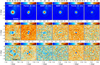 |
Fig. A.1. WMAP and Planck-LFI total intensity (top row) and polarisation (middle row Stokes Q, bottom row Stokes U) maps at the position of the SNR Cas A. The Q and U polarisation maps show the cloverleaf-shaped pattern typical of beam polarisation. The solid and dashed circles denote the regions we have used for aperture photometry integration and background subtraction to derive the values quoted in Tables A.1 and A.2. |
Level of leakage in WMAP computed on three bright unpolarised regions.
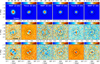 |
Fig. A.2. WMAP and Planck-LFI total intensity (top row) and polarisation (middle row Stokes Q, bottom row Stokes U) maps at the position of the HII region M42. As in Fig. A.1, the Q and U polarisation maps show the cloverleaf-shaped pattern typical of beam polarisation. The solid and dashed circles denote the regions we have used for aperture photometry integration and background subtraction to derive the values quoted in Tables A.1 and A.2. |
Level of leakage in Planck-LFI maps computed on three bright unpolarised regions.
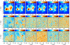 |
Fig. A.3. WMAP and Planck-LFI total intensity (top row) and polarisation (middle row Stokes Q, bottom row Stokes U) maps at the position of the Cygnus X molecular complex. Some Stokes Q and U maps show residual polarisation probably associated with spurious intensity leakage produced by bandpass mismatch. The unshaded regions in the top row indicate the pixels that are used in the correlation plot analysis (see the main text for details). |
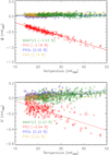 |
Fig. A.4. Stokes parameters Q (top) and U (bottom) versus total intensity signal in the Cygnus X star-forming complex. With different colours we represent WMAP 23 GHz (green) and Planck-LFI 30 GHz data for three different cases: PR3 raw (un-corrected) data (red), PR3 leakage-corrected data (blue) and PR4 leakage-corrected data (gold). In the legend we quote the Q/I and U/I polarisation fractions derived from the linear-regression fits represented by the solid lines (same values that are quoted in Tables A.2 and A.1.). |
Appendix B: Tables
Data used in this paper.
Main parameters of the raster scan observations of each field.
Total integration times and final sensitivities in each field and at all frequency bands.
Intensity flux densities for ρ Ophiuchi, Perseus, and W43 obtained through aperture photometry on maps degraded to a common angular resolution of 1°.
Anomalous microwave emission (between frequencies 11.1 and 44.1 GHz) and thermal dust (frequencies 60.5 to 353 GHz) polarisation constraints on ρ Ophiuchi.
Same as Table B.5 but for Perseus.
Same as Table B.5 but for W43.
All Tables
Level of leakage in Planck-LFI maps computed on three bright unpolarised regions.
Total integration times and final sensitivities in each field and at all frequency bands.
Intensity flux densities for ρ Ophiuchi, Perseus, and W43 obtained through aperture photometry on maps degraded to a common angular resolution of 1°.
Anomalous microwave emission (between frequencies 11.1 and 44.1 GHz) and thermal dust (frequencies 60.5 to 353 GHz) polarisation constraints on ρ Ophiuchi.
All Figures
|
Fig. 1. Left: QUIJOTE-MFI wide survey intensity map at 11 GHz (Rubiño-Martín et al. 2023) with the locations of the three regions studied in this paper overlaid. Right: Map of the number of hits (per pixel of HEALPixNside = 512 and in units of seconds) for horn 3 11 GHz after combination of the wide survey data in nominal mode with the raster scan data listed in Table B.2. |
| In the text | |
|
Fig. 2. High-angular resolution maps from Planck-HFI 857 GHz around the positions of the three studied regions. In the case of the ρ Ophiuchi and Perseus molecular clouds we indicate the positions of different compact clouds extracted from different catalogues and the location of the main ionising star. In W43 we indicate the positions of the molecular clouds identified in the CO survey of Solomon et al. (1987), highlighting in red the two most massive ones. The solid circle delineates the aperture used for flux density integration and the dashed circles enclose the ring used for background subtraction (see Sect. 4.1). |
| In the text | |
|
Fig. 3. Intensity and polarisation maps around the ρ Ophiuchi molecular cloud from QUIJOTE-MFI and from the two lowest-frequency bands of WMAP and Planck. The three rows show respectively I, Q and U maps, while the columns correspond to 11, 13, 17 (Horn 2), 19 (Horn 2), 23 and 30 GHz from left to right. The solid circle shows the aperture we used for flux integration, whereas the two dashed circles enclose the ring we used for background subtraction. The small circle inside the background annulus towards the west indicates the mask applied to avoid a strong HII source. The grey areas towards the southwest at 17 and 19 GHz are masked due to satellite contamination. For the sake of better visualisation, these maps are shown at their raw angular resolution, although all the analyses presented in this paper have been performed on maps convolved to a common angular resolution of 1°. |
| In the text | |
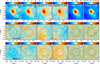 |
Fig. 4. Same as Fig. 3 but for the Perseus molecular cloud. |
| In the text | |
|
Fig. 5. Intensity and polarisation maps around the W43 molecular cloud. The three rows show, respectively, I, Q, and U maps, while the columns correspond to QUIJOTE-MFI 17 (Horn 2) and 19 GHz (Horn 2) and to WMAP 23 GHz, from left to right. The solid circle shows the aperture we used for flux integration, whereas the two dashed circles enclose the ring we used for background subtraction. |
| In the text | |
|
Fig. 6. Example of a corner plot of the two-dimension parameter space explored by the MCMC implemented in the EMCEE package corresponding to the W43 molecular complex. Blue and red contours correspond respectively to the fits with and without QUIJOTE data (see derived best-fit parameters in Table 3). Also shown are one-dimension marginalised posterior distributions from which the best-fit parameters and uncertainties are determined. |
| In the text | |
|
Fig. 7. Illustration of the effect of the polarisation leakage correction in Planck-LFI at 28.4 GHz around the position of W43. Stokes Q and U maps are represented respectively in the top and bottom panels. From left to right, the panels respectively show the PR3 raw (un-corrected) maps, the PR3 leakage-corrected maps using our own implementation (see Sect. 4.4.2 for details), and the public PR4 corrected maps. |
| In the text | |
|
Fig. 8. Intensity and polarisation stacked I, Q, and U maps at a reference frequency of 22.8 GHz and at the position of the three sources studied in this paper. These maps are the result of a weighted average of maps at frequencies around the AME peak frequency convolved at a common angular resolution of 1° and were obtained following the procedure outlined in Sect. 4.4.3. |
| In the text | |
|
Fig. 9. ρ Ophiuchi intensity SED. QUIJOTE-MFI data points are depicted in red together with other ancillary data (blue), including WMAP 9-yr (green), Planck (orange), and COBE-DIRBE data (light green). At intermediate frequencies, the excess emission associated with the AME clearly shows up. A joint fit has been performed consisting of the following components: free-free (orange line), AME log-normal model (purple line), CMB (blue line), and thermal dust (green-olive line). The black line represents the sum of all components. |
| In the text | |
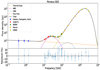 |
Fig. 10. Same as Fig. 9 but for Perseus. |
| In the text | |
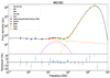 |
Fig. 11. Same as Fig. 9 but for W43. |
| In the text | |
|
Fig. A.1. WMAP and Planck-LFI total intensity (top row) and polarisation (middle row Stokes Q, bottom row Stokes U) maps at the position of the SNR Cas A. The Q and U polarisation maps show the cloverleaf-shaped pattern typical of beam polarisation. The solid and dashed circles denote the regions we have used for aperture photometry integration and background subtraction to derive the values quoted in Tables A.1 and A.2. |
| In the text | |
|
Fig. A.2. WMAP and Planck-LFI total intensity (top row) and polarisation (middle row Stokes Q, bottom row Stokes U) maps at the position of the HII region M42. As in Fig. A.1, the Q and U polarisation maps show the cloverleaf-shaped pattern typical of beam polarisation. The solid and dashed circles denote the regions we have used for aperture photometry integration and background subtraction to derive the values quoted in Tables A.1 and A.2. |
| In the text | |
|
Fig. A.3. WMAP and Planck-LFI total intensity (top row) and polarisation (middle row Stokes Q, bottom row Stokes U) maps at the position of the Cygnus X molecular complex. Some Stokes Q and U maps show residual polarisation probably associated with spurious intensity leakage produced by bandpass mismatch. The unshaded regions in the top row indicate the pixels that are used in the correlation plot analysis (see the main text for details). |
| In the text | |
|
Fig. A.4. Stokes parameters Q (top) and U (bottom) versus total intensity signal in the Cygnus X star-forming complex. With different colours we represent WMAP 23 GHz (green) and Planck-LFI 30 GHz data for three different cases: PR3 raw (un-corrected) data (red), PR3 leakage-corrected data (blue) and PR4 leakage-corrected data (gold). In the legend we quote the Q/I and U/I polarisation fractions derived from the linear-regression fits represented by the solid lines (same values that are quoted in Tables A.2 and A.1.). |
| In the text | |
Current usage metrics show cumulative count of Article Views (full-text article views including HTML views, PDF and ePub downloads, according to the available data) and Abstracts Views on Vision4Press platform.
Data correspond to usage on the plateform after 2015. The current usage metrics is available 48-96 hours after online publication and is updated daily on week days.
Initial download of the metrics may take a while.