| Issue |
A&A
Volume 695, March 2025
|
|
|---|---|---|
| Article Number | A77 | |
| Number of page(s) | 20 | |
| Section | Interstellar and circumstellar matter | |
| DOI | https://doi.org/10.1051/0004-6361/202451430 | |
| Published online | 12 March 2025 | |
Investigating ultraviolet and infrared radiation through the turbulent life of molecular clouds
1
Scuola Normale Superiore,
Piazza dei Cavalieri 7,
56126
Pisa, Italy
2
Center for Computational Astrophysics, Flatiron Institute,
162 5th Avenue,
New York,
NY
10010,
USA
3
Institute of Theoretical Astrophysics, University of Oslo,
PO Box 1029, Blindern 0315,
Oslo, Norway
★ Corresponding author; fabio.dimascia@sns.it
Received:
9
July
2024
Accepted:
31
January
2025
Context. Molecular clouds (MCs) are the places where stars are formed and their feedback starts to take place, regulating the evolution of galaxies. Therefore, MCs represent the critical scale at which to study how ultraviolet (UV) photons emitted by young stars are reprocessed in the far-infrared (FIR) by interaction with dust grains, thereby determining the multiwavelength continuum emission of galaxies.
Aims. Our goal is to analyze the UV and IR emission of a MC at different stages of its evolution and relate its absorption and emission properties with its morphology and star formation rate. Such a study is fundamental to determining how the properties of MCs shape the emission from entire galaxies.
Methods. We considered a radiation-hydrodynamic simulation of a MC with self-consistent chemistry treatment. The MC has a mass of MMC = 105 M⊙, is resolved down to a scale of 0.06 pc, and evolves for ≃2.4 Myr after the onset of star formation. We post-processed the simulation via Monte Carlo radiative transfer calculations to compute the detailed UV-to-FIR emission of the MC. Such results were compared with data from physically motivated analytical models, other simulations, and observations.
Results. We find that the simulated MC is globally UV-optically thick, but optically thin channels allow for photon escape (0.1–10%), a feature that is not well captured in analytical models. The dust temperature spans a wide range (Tdust ∼ 20–300 K) depending on the dust-to-stellar geometry, which is reproduced reasonably well by analytical models. However, the complexity of the dust temperature distribution is not captured in the analytical models, as is evidenced by the 10 K (20 K) difference in the mass (luminosity) average temperature. Indeed, the total IR luminosity is the same in all the models, but the IR emission peaks at shorter wavelengths in the analytical ones. Compared to a sample of Galactic clouds and other simulations, our spectral energy distribution (SED) is consistent with mid-IR data, but peaks at shorter wavelengths in the IR. This is due to a lack of cold dust, as a consequence of the high gas – and thus dust – consumption in our simulated MC. The attenuation properties of our MC change significantly with time, evolving from a Milky-Way-like relation to a flatter, featureless one. On the IRX-β plane, the MC position strongly depends on the observing direction and on its evolutionary stage. When the MC starts to disperse, the cloud settles at log(IRX) ∼ 1 and β ∼ −0.5, slightly below most of the local empirical relations.
Conclusions. This work represents an important test for MC simulations and a first step toward the implementation of a physically informed, sub-grid model in large-scale numerical simulations to describe the emission from unresolved MC scales and its impact on the global galaxy SED.
Key words: radiative transfer / methods: numerical / ISM: clouds / dust, extinction / ISM: general
© The Authors 2025
 Open Access article, published by EDP Sciences, under the terms of the Creative Commons Attribution License (https://creativecommons.org/licenses/by/4.0), which permits unrestricted use, distribution, and reproduction in any medium, provided the original work is properly cited.
This article is published in open access under the Subscribe to Open model. Subscribe to A&A to support open access publication.
1 Introduction
Molecular clouds (MCs) are the birthplaces of stars. Gas in over- dense regions within MCs cools and collapses until the density is high enough to trigger star formation (SF). This process is regulated by the interaction between the pressure support of the turbulence motions and the gravitational force, which allows for the formation of filaments and clumps (e.g., Zuckerman & Evans 1974; Brunt et al. 2009; Krumholz et al. 2012; Colombo et al. 2014; Dobbs 2015). The newly formed stars emit photons that heat and ionize the surrounding interstellar medium (ISM), altering the molecular gas reservoir available for SF (e.g., Whitworth 1979). Furthermore, M⋆ > 10 M⊙ stars affect the ISM via stellar winds (e.g., Castor et al. 1975; Weaver et al. 1977) and then end their lives as supernova explosions after ∼10 Myr (e.g., Sedov 1958; Ostriker & McKee 1988), injecting thermal energy and momentum into the ISM. The effect of stellar feedback is essential in determining the complex structure of MCs, their evolution, and ultimately the star formation efficiency (SFE or ϵ⋆); that is, the fraction of gas converted into stars during the MC lifetime1.
Observations of MCs in the Milky Way (MW) suggest low values for the star formation rate (SFR) and consequently SFEs of only a few percent (Zuckerman & Palmer 1974; Evans et al. 2009; Forbrich et al. 2009; García et al. 2014; Louvet et al. 2014; Chevance et al. 2020), with the most active clouds being able to convert ∼10% of their gas mass into stars (e.g., Lee et al. 2016). These observations probe the dust grains in the cold, dense gas within the MCs, which obscure optical starlight and re-emit it at longer wavelengths, from the near-infrared (NIR) to the submillimeter band. Through this emission, infrared (IR) surveys with Spitzer and Herschel (e.g., Churchwell et al. 2009; Molinari et al. 2010) have provided the first view of the clumps and filaments in the MW plane, providing a picture of SF in our Galaxy.
From a theoretical point of view, MCs can be studied by analytical means (e.g., Whitworth 1979; Williams & McKee 1997; Matzner 2002; Krumholz et al. 2012; Vázquez-Semadeni et al. 2019), which can pinpoint the relevant physical process responsible for the evolution of MCs, and numerical simulations, which can account for the complex structure of MCs and better constrain the interplay of SF and stellar feedback (e.g., Kim & Ostriker 2017; Jeffreson et al. 2024), for instance focusing on the impact of radiation (e.g., Decataldo et al. 2020; Menon et al. 2023), stellar winds (e.g., Geen et al. 2021; Lancaster et al. 2021a,b), the role of magnetic field in shaping the MC structure (e.g., Federrath & Klessen 2012; Hennebelle et al. 2022), or the influence of the galactic (large-scale) environment on cloud formation (e.g., Butler et al. 2015; Smith et al. 2020).
A fundamental ingredient in numerical simulations is the modeling of radiation from stars. In particular, M★ > 5 M⊙ stars emit a copious amount of photons in the far-ultraviolet (FUV; 6 eV < hv < 13.6 eV), which can dissociate CO and H2 molecules, and in the extreme-ultraviolet (EUV; hv > 13.6 eV), which ionize hydrogen and helium. The difference in pressure between the hot, ionized gas and the cold, molecular ISM leads to the propagation of shocks ahead of dissociation and/or ionization fronts, compressing the gas and driving turbulent motions (e.g., Kahn 1954; Williams et al. 2018), possibly opening channels through which Lyman continuum and Lyman-α photons can leak out of the MC (e.g., Kakiichi & Gronke 2021). Although dense clumps lose their mass due to gas photo-evaporation, at the same time, radiation-driven compression can also trigger SF (e.g., Kessel-Deynet & Burkert 2003; Dale et al. 2005; Bisbas et al. 2011; Decataldo et al. 2019, 2020). Accurate modeling of this complex interplay between stellar radiation and gas dynamics is therefore essential to investigate the SFR within an MC.
However, despite great recent progress, there are still limitations in current theoretical models. Radiation hydrodynamic (RHD) simulations implement radiative transfer (RT) on the fly with only a select number of energy bins, because of the high computational costs (e.g., Decataldo et al. 2020), with some notable exceptions (e.g., Ali 2021). Therefore, only a small portion of the total spectral energy distribution (SED) of the MCs is accessible, and with poor wavelength resolution. Moreover, dust treatment is rarely included in these simulations, so radiation reprocessing by dust grains is usually not accounted for. As MCs are typically observed in IR bands (e.g., Lin et al. 2017; Binder & Povich 2018; Ladjelate et al. 2020; Potdar et al. 2022), it is essential to have a tool to model the full UV-to-FIR SED, including the dust contribution, to effectively benchmark theoretical models against observations.
A common framework to achieve this task is to compute the propagation of radiation in post-processing to produce synthetic observations that can be directly compared with observations, a strategy widely adopted in the context of galaxy environment simulations (e.g., Camps et al. 2016; Koepferl & Robitaille 2017; Behrens et al. 2018; Haworth et al. 2018; Cochrane et al. 2019; Reissl et al. 2020; Di Mascia et al. 2021). Such synthetic observations can serve multiple purposes. They can be used to test the robustness of hydrodynamic simulations in reproducing the structure and physical properties of MCs, and conversely they can also be used to quantify the limits of current observational techniques in inferring the physical properties of MCs.
Recently, Jáquez-Domínguez et al. (2023, hereafter JD23) performed RT calculations in post-processing and produced synthetic observations of the MCs formation simulations presented in Zamora-Avilés et al. (2019), featuring a young star cluster with massive SF and ionization feedback. They explored the evolution of the SED as the cloud morphology changes due to the effect of ionizing photons, which leads to the expansion of HII regions and the formation of cavities. These results emphasize how complex, varied, and sensitive to the observing direction the galaxy emission is at scales below ≈10 pc. These spatial scales are currently unresolved in cosmological hydrodynamic simulations of galaxy formation, both large-scale (Schaller et al. 2015; Feng et al. 2016; Pillepich et al. 2018; Kannan et al. 2022) and zoom-in (Ceverino et al. 2017; Hopkins et al. 2018; Lovell et al. 2021; Pallottini et al. 2022). Therefore, most of the observable predictions derived from these simulations (e.g., UV escape fraction, UV luminosity function, IRX-β relations, etc.) are limited by the lack of resolution on small scales.
In this work, we aim to take a first step toward improving the description of UV and IR continuum emission in simulations of the ISM at the scale of MCs. We do so by comparing the results of post-processed RHD simulations of a local MC with physically informed analytical models, with the long-term goal of implementing them as sub-grid models in numerical simulations. We investigate the multiwavelength emission of local MCs, making use of the RHD simulation performed in Decataldo et al. (2020, hereafter D20). This simulation follows the evolution of a MC, implementing on-the-fly RT with ten radiation bins and a chemical network including H2 formation and destruction, to self-consistently model SF and stellar feedback. We perform RT calculations in post-processing using the Monte Carlo RT code SKIRT (Camps & Baes 2015, 2020) to study the multiwavelength emission from the MC, the UV escape fraction, the dust properties (e.g., dust attenuation and dust grain temperature distribution), and how the MC physical properties (e.g., SF, morphology) impact its emission throughout its evolution. We also make use of the analytical models of MC emission by Sommovigo et al. (2020, hereafter S20) to explore how simple physically motivated prescriptions capture the MC properties of modern RHD simulations. This is a starting point toward the development of a model to describe the structure and the emission of unresolved structures on sub-grid scales (< 1 pc) in galaxy simulations.
The paper is organized as follows. In Sect. 2, we describe the numerical and theoretical models adopted. In particular, in Sect. 2.1 we present the hydrodynamic simulations; in Sect. 2.2 we illustrate the details of the post-processing RT setup; and in Sect. 2.3 we describe the analytical model from S20. In Sect. 3, we analyze in detail the properties of the MC at a specific snapshot, which we consider as a reference snapshot. In Sect. 4, we study the evolution of the physical and emission properties of the MC. Finally, we conclude in Sect. 5.
2 Model
2.1 Molecular cloud evolution
The radiation-hydrodynamic MC model is fully described in D20 and summarized here.
2.1.1 Simulation setup
Simulations were carried out using a customized version of the adaptive mesh refinement code RAMSES (Teyssier 2002), which uses a second-order Godunov scheme for the gas hydrodynamics and a particle-mesh solver for particles as stars, solving self-gravity with a multigrid solver (Guillet & Teyssier 2011).
In D20, the full box size is 60 pc, and the resolution ranges from Δx ≃ 0.9 pc to Δx ≃ 0.06 pc, according to a semi-Lagrangian strategy.
Radiation was evolved with the RAMSES-RT module (Rosdahl et al. 2013) by adopting a first-order Godunov solver with a M1 closure relation (Aubert & Teyssier 2008). In D20, ten radiation energy bins were tracked, from 0.75 eV to 54.42 eV, covering the transition energy of the nine photoreactions included in the chemical network. It should be noted that D20 uses a reduced speed of light approximation, cred = 10−3 c, which yields an inaccurate propagation of the ionization front when its speed is larger than cred , which in the simulation happens only close to very massive stars (cf. Deparis et al. 2019; Decataldo et al. 2019; Pallottini et al. 2022).
Nonequilibrium chemistry was accounted for by using KROME (Grassi et al. 2014), with a chemical network accounting for nine species (H, H+, H−, H2,  , He, He+, He++ and free electrons), 46 reactions (see Bovino et al. 2016; Pallottini et al. 2017 for details), and fully coupled with the RAMSES-RT module (Pallottini et al. 2019; Decataldo et al. 2019). The formation of H2 molecules, which mainly happens on the surface of dust grains, is regulated by the gas and dust temperature in the RHD simulation, following the rate given by Hollenbach & McKee (1979) and Sternberg & Dalgarno (1989). In the chemistry module, the dust temperature is assumed to be constant at Td = 30 K. Several gas heating and cooling mechanisms were also included. Heating is provided by photo-heating of H and He (computed as in Sect. 2.2 of Grassi et al. 2014), photo-electric heating from dust, heating from exoenergetic reactions, and cosmic rays2). Gas cooling is driven by collisional ionization, collisional excitation and recombination of H and He (rates from Cen 1992), free-free cooling, cooling by H2 (Glover & Abel 2008) and metal cooling, obtained with CLOUDY (version 10.00 Ferland et al. 1998). No interstellar radiation field (ISRF) was assumed a priori, and the radiation field was computed on the fly as was specified above.
Initially, the cloud has a mass MMC = 105 M⊙, a radius RMC = 20 pc (average number density of n = 120 cm−3), a constant Zgas = Z⊙ = 0.02 metallicity (defined as the sum of the heavy metals relative to the total gas mass) and a dust-to-metal ratio of fd = 0.3 (Mdust = 6.4 × 10² M⊙; see Sect. 2.2 for the dust properties), which is appropriate for a MC in the MW (e.g., Heyer et al. 2009). The MC has a turbulent velocity field set up such that the virial parameter  ; in other words, it is marginally unstable. Further, the MC is embedded in a low-density medium (n = 1 cm−3) set in pressure equilibrium. These initial conditions are evolved for 3 Myr before the cloud is allowed to form stars.
2.1.2 Star formation and stellar feedback
In D20, stars can form according to a local Schmidt (1959); Kennicutt (1998) relation; for each star, the mass (m⋆) was drawn from a pre-computed Kroupa (2001) initial mass function, where stars with m ≤ 1 M⊙ were removed for computational efficiency. In D20, the SFR and the gas mass within the MC were corrected a posteriori to take into account the low-mass stars excluded in the simulation. While including small mass stars can slightly alter the gas dynamic, their feedback is expected to be subdominant, particularly regarding their contribution to the UV radiation, and therefore to the dust heating (see Sect. 2.2 and in particular footnote 5). For this reason throughout this paper, we adopt the uncorrected SFR and we consider only stars spawned in the hydrodynamic simulation as radiation sources in the RT post-process.
In the simulation, stars act as radiation point sources and, if massive enough, can inject energy and mass via winds. D20 adopts evolutionary tracks from PARSEC (Bressan et al. 2012) and atmospheric models from Castelli & Kurucz (2003), in order to compute the mass loss rate, the wind kinetic power, the bolometric luminosities and the spectral shapes. The wind feedback scheme allows for energy and momentum injection into the cells surrounding massive stellar particles (Gatto et al. 2017; Haid et al. 2018).
In Fig. 1, we show the SFR in the D20 MC as a function of time. We note that we do not account for the low-mass stars correction to the SFR in the plot (see Sect. 2.2 in D20 for details). The SFR increases from ≃10−3 M⊙ yr−1 to a peak of 0.15 M⊙ yr−1 at t ≃ 1.8 Myr; at t ≃ 1.7 Myr the cloud starts to photo-evaporate (vertical dashed line in Fig. 1); in other words, the gas starts to be ejected from the cloud by winds and radiation pressure, quenching the SFR a few million years afterward. At this stage, it has a stellar mass of M★ = 2.2 × 10⁴ M⊙ (M★ = 4.3 × 10⁴ M⊙ if accounting also for low-mass stars). It should be noted that the SFR is particularly bursty at early times, with stochastic variation up to 1 dex, and the amplitude of the fluctuations becomes negligible around the t ≃ 1.5 Myr mark (cf. Furlanetto & Mirocha 2022; Pallottini & Ferrara 2023; Sun et al. 2023, for SFR variations in galaxies).
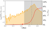 |
Fig. 1 Star formation rate (SFR, orange) and instantaneous SFE (є★(t) = M★(t)/MMC, red), as a function of time (t) for the MC from D20. At the end of the simulation, the total mass in stars is M★ = 7.4 × 10⁴ M⊙. The circles mark the time corresponding to the “reference” snapshot (as defined in Sect. 3), at t ≃ 1.1 Myr. The dashed vertical line indicates the moment when the MC in D20 starts to photo-evaporate. The shaded area highlights the period when the cloud is dispersed according to the radiation–pressure model from S20 (cf. Sect. 2.3.) . |
2.2 Radiative transfer through dust in MCs
The on-the-fly RT module included in the simulations by D20 allows us to model self-consistently the propagation of radiation and the gas chemical evolution. However, the number of energy bins is too low to make solid predictions for the SED of the MC. For this reason, we post-processed the MC with 3D RT calculations by adopting version 9 of the Monte Carlo code SKIRT3 (Camps & Baes 2015, 2020).
SKIRT includes a full treatment of absorption and scattering of light by dust grains, and it calculates self-consistently the dust thermal emission. The code can handle arbitrary threedimensional geometries for both the radiation sources and the dust component, and it includes a large variety of emission models for the sources. Further, SKIRT has been widely used to generate precise synthetic observations of simulated galaxies (e.g., Camps et al. 2016; Trayford et al. 2017; Behrens et al. 2018; Cochrane et al. 2019; Liang et al. 2021; Vijayan et al. 2022), AGN-hosts (e.g., Viaene et al. 2020; Di Mascia et al. 2021, 2023), and recently it has also been applied to simulations of Galactic MCs (see JD23).
A RT calculation with SKIRT requires two main ingredients: a source component, which determines the intrinsic radiation field within the computational domain, and a dust component, which alters the radiation via scattering and absorption, and then thermally re-emits photons, reshaping the radiation field.
2.2.1 Stellar emission
We imported the individual stars in the hydrodynamic simulation. Consistently with D20, their SED was computed based on the stellar atmosphere models by Castelli & Kurucz (2003), which depend on the stellar metallicity, Z⋆ , the surface temperature, T⋆ and the surface gravity, ɡ⋆4. We used the stellar evolutionary tracks computed with the PARSEC code (Bressan et al. 2012) to relate the temperature T⋆ and radius R⋆ of each star to its mass m⋆ , assuming that all the stars have the same metallicity as the gas; that is, Z★ = Zgas = Z⊙. We underline that, by importing only the stars included in the hydrodynamic simulation, only radiation from stars with m★ > 1 M⊙ is considered in the RT calculation5. These stars are the ones contributing to the SFR and total stellar mass budget M⋆ shown in Fig. 1.
We do not include a contribution from an ISRF as an additional radiative source. JD23 noted that not including ISRF might result in dust temperatures unrealistically low (≈4 K) in the early stages of the cloud evolution, when massive stars are yet to form. At these times, the MC is expected to have temperatures typical of IR dark clouds (≈10 K; Rathborne et al. 2006; Pillai et al. 2011). JD23 found that with the inclusion of a radiation field of LISRF = 104 L⊙ (comparable to the stellar emission at early times in their simulation), they were able to obtain a mass- weighted dust temperature of 8.7 K for their earliest snapshot. In our case, the median of the mass-weighted dust temperature is 9.8 K (cf. Fig. 8) for the first snapshot analyzed, when the intrinsic luminosity from stars is ≃8.5 × 10⁴ L⊙, a factor of ≈10 larger than in JD23. Therefore, we argue that the inclusion of an ISRF would not affect significantly the dust temperature distribution in our simulations.
2.2.2 Dust distribution and properties
We imported in SKIRT the octree structure of the hydrodynamic simulation. We assigned to each cell a dust mass content by rescaling the gas metal mass with a dust-to-metal ratio of fd = 0.3, consistently with the chemistry model adopted in D20. In cells with high gas temperature (T ≳ 106K, see e.g., Di Mascia et al. 2021), grains are efficiently destroyed via thermal sputtering, as collisions with ions are expected to be more frequent. However, we find this effect to be relevant for ≲0.1% of the total dust mass in our simulations, so we do not apply any dust destruction recipe in the pre-process.
For the dust optical properties, we used the MW model from Weingartner & Draine (2001) with the visual extinction- to-reddening ratio equal to RV = 3.1. The dust mix consists of graphite, silicate, and polycyclic aromatic hydrocarbon (PAH) grains, whose size distribution spans from 3.5 × 10⁻⁴ µm to 10 µm. Each component is discretized in 10 bins for the computation.
2.2.3 SED modeling
We restricted the simulated spectra to the wavelength range 0.09–1000 µm, sampled by a grid with 200 bins distributed with a logarithmic spacing. The limits were chosen to include the UV and optical photons for which the dust absorption/scattering cross sections are higher and all the relevant wavelengths for the primary emission from stars. We did not include photons below 0.09 µm because we expect hydrogen absorption to be more important than dust in that regime.
SKIRT performs the RT computation in two stages. First, it propagates radiation from the primary sources (i.e., stars). The absorbed radiation and the resulting radiation field are then used to compute the temperature of each grain population in each cell in the computational domain6. In the second stage, the dust thermal emission is propagated; that is, dust cells act as radiative sources. Their emission can further interact with the dust component if the density is high enough that the dust optical depth is non-negligible at longer wavelengths, changing in turn the dust thermal state. Therefore this computation is repeated until a convergence criterion is satisfied. We stop the iteration when the total absorbed dust luminosity changes by less than 3% with respect to the previous step. We used 5 × 10⁶ photon packets for our simulations, 50% being equally distributed among different sources, 50% being preferentially assigned to higher luminosity sources. We discuss the convergence of our results with respect to this choice in Appendices B and C.
2.2.4 Sample selection
We selected a total of 24 snapshots to be post-processed, from t = 0.08 Myr to t = 2.34 Myr since the beginning of SF in the cloud, to probe all the different stages of the cloud evolution. In SKIRT, it is possible to configure an instrument, which acts as a synthetic detector, to collect radiation from the computational domain. For the detector, we adopt the same wavelength grid used in the RT computation. We place a total of 6 detectors at different angular positions around the simulated box to explore variations in the emission of the simulated cloud with the observing direction. In particular, each detector faces perpendicular to each of the six faces of the simulated cubic box. One of them is chosen as the reference observing direction to study the cloud emission. Throughout the paper, we refer to the direction pointed at by the detectors as the “observing direction”. Each detector has a field of view of 60 pc × 60 pc, which covers the entire face of the computational box, and 1024 × 1024 pixels, in order to match the maximum physical resolution of the hydrodynamic simulation.
2.3 An essential model for dust emission in MCs
In this work, we adopt the model from S20 as the main tool for comparisons. The physically motivated model for computing dust emission from MCs from S20 is summarized below, along with the modification needed to have a closer match with the D20 MC setup.
In S20, MCs are modeled assuming spherical symmetry and are characterized by a mass MMC equal to the Jeans mass with a number density of n ≃ 122 cm−3, a radius RMC given by the Jeans length, and a supersonic velocity dispersion σMC . In the present, RMC and MMC are the same as S20, which are close to the values of the MC in D20; σMC is set such that α = 5/3 and the dust mass matches the one in D20.
Stars are located at the center of the MC and their radiation is absorbed by the dust as it travels outward; to this end, the cloud is divided in optically thin shells, containing a fraction of dust with a grain size distribution according to the Milky-Way model by Weingartner & Draine (2001). As the UV radiation from the stars is absorbed by dust, it emits as a modified black body, with a temperature dependence on the absorbed luminosity and grain size, assuming local thermal equilibrium (LTE). In the original S20 publication, stars are allowed to form with a Schmidt (1959)- Kennicutt (1998) relation and the UV radiation was computed with STARBURST99 (Leitherer et al. 1999). In this work, we use the stars in the simulation as radiative sources for the S20 model, in order to match the UV SED and intensity field with D20.
The system can be solved once the density profile is specified. S20 adopts either a homogeneous density (“homogeneous” model) or the profile resulting from the impact of radiation pressure due to the presence of H II regions (Draine 2011, “radiation–pressure” model). In the latter case, the mass that is pushed outside the cloud radius due to the radiation pressure is assumed to be lost. Therefore, the total dust mass in the radiation–pressure case tends to be smaller than in the homogeneous case, as the cloud evolves.
3 A closer look at a prototypical MC
As a first step in our investigation of the emission properties of the evolving MC, we focus on a snapshot at t ≈ 1.1 Myr (after the beginning of SF), which we refer to as our “reference” snapshot. At this stage, the MC has a (uncorrected) stellar mass of M★ ~ 2.3 × 10³ M⊙ and a SFR ~ 0.01 M⊙ yr−1 (cf. Fig. 1). The choice of this snapshot was motivated by the need to investigate the cloud after SF has proceeded for enough time for stellar feedback to be effective. Another reason to use this snapshot was that photo-evaporation is over-estimated when using the radiation–pressure model by S20 with the D20 SED as all the stars are placed in the center of the cloud, and the cloud becomes effectively dispersed after t = 1.2 Myr, making a comparison between the analytic models and the simulated MC less meaningful. Throughout the paper, the time when the cloud is dispersed in the radiation–pressure model is emphasized with a shaded gray area. We now discuss the cloud morphology at the reference snapshot in Sect. 3.1, then its emission properties in Sect. 3.3, and the dust temperature distribution in Sect. 3.4.
3.1 Cloud morphology and dust mass distribution
In Fig. 2, we provide an overview of the complex MC morphology at the reference evolutionary stage, by zooming on the central 20 × 20 pc2 of the simulated box. At this stage, massive stars have already produced enough ionizing photons to form H II bubbles around them, and their feedback-driven turbulence led to the formation of filamentary structures of neutral gas.
The dust surface density (top left panel) is distributed into several filaments with densities Σdust ≳ 10 M⊙ pc−2, in contrast with lower-density regions at 1 M⊙ pc−2; a few clumps are also visible where filaments intersect each other. We also show the positions of the 729 stars in place at this epoch, with a mass between 1–84 M⊙, and a total stellar mass of M★ = 2.4 × 10³ M⊙. Many stars reside along dense filaments, but some of them have already cleared the surrounding gas with stellar feedback. The top center panel illustrates the photon density-weighted Habing flux G0 (6eV < hν < 13.6eV) computed on the fly in the D20 simulation; the patchy distribution of the Habing flux reflects the impact of stellar radiation in their close surroundings, with high-mass stars imprinting their radiative feedback over larger distances, also because of stellar winds decreasing the gas density in the immediate vicinity of stars. At this resolution, the G0 flux spans seven orders of magnitude (100–107), with a skewed distribution toward large values, as is seen by looking at the quantiles of the distribution; that is, 〈G0〉 =  . The top right panel illustrates the photon density-weighted ionizing flux, Uion (hν > 13.6 eV), computed on the fly in the D20 simulation. It shows a patchy morphology that emphasizes the regions where the radiative feedback from the most massive stars acted. Uion spans a wide range (10−1–105), with a skewed distribution toward large values:
The bottom left and middle panels show the morphology of the MC emission in the UV (0.1–0.3 µm) and IR (8–1000 µm) bands. These maps were smoothed with a Gaussian kernel of σ = 1 pixel with respect to the original resolution for visualization purposes only. The UV emission toward the reference observing direction shows a diffuse component at SUV ~ (1– 10) × 10−4 L⊙ kpc−2, with a few pixels with high values (SUV ≳ 1 L⊙ kpc−2) corresponding to the locations of unobscured luminous stars. Dust attenuation plays a major role in shaping the UV emission, since only LUV ≃ 3.76 × 10⁵ L⊙ is collected toward the reference observing direction, corresponding to the ≃12.7%8 of the intrinsic luminosity of LUV,int ≃ 2.95 × 10⁶ L⊙. Most of this emission comes from stars whose stellar feedback has cleared out the surrounding gas. This trend is even more apparent by looking at the distribution of the UV optical depth τUV9, which shows several peaks corresponding to dust-obscured stars embedded inside small high-density clumps or filaments. The optical depth distribution has a pixel-based median of τUV =  , thus most stars are optically thick in the UV band, with extreme peaks at τUV > 10. The IR emission from dust thermal radiation features a spatial distribution that resembles the dust surface density distribution, with similar filamentary structures characterized by SIR ~ 10−2–10−1 L⊙ kpc−2. One highly emitting (SIR ≳ 10 L⊙ kpc≳2) spot is also visible, corresponding to a dusty region irradiated by close stars, which end up being completely dust-obscured in the UV. The total IR luminosity is LIR ≃ 3.0 × 10⁶ L⊙, showing that most of the intrinsic radiation coming from the stars is re-emitted in the IR10, due to the presence of dust giving a high τUV.
We now discuss the cloud morphology in a more quantitative way. In Fig. 3, we show the cumulative radial mass profile for the dust and stars (normalized to their respective total mass). The stellar component is more compact than the dust component, with the 90% of the total stellar mass enclosed in a radius of r*,90 ≃ 7.4 pc and rdust,90 ≃ 13 pc, respectively. However, the two profiles are quite similar and reach a plateau at the same radius, emphasizing that SF follows the gas mass distribution. As a reference, we also report the mass profile for the S20 model in the uniform density case and in the radiation–pressure case. In the homogeneous case, the dust mass distribution is by construction ∝ r3, and it is less concentrated in the inner ~10 pc of the MC with respect to the D20 simulations; however, the radius containing 90% of the total dust mass is comparable, with  pc. In the radiation-pressure case, the central region is almost deprived of their content as dust is pushed away. The mass profile recovers the shape of the homogeneous case only at r ≈ 7 pc. However, the radius containing 90% of the total mass is comparable,
  . The total dust mass retained in the radiation-pressure case is 1.7 × 10²M⊙, as the H II region almost reaches the outer edge of the cloud.
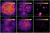 |
Fig. 2 Morphology of the MC at the reference snapshot, zooming on the central region of the box with a side length of 20 pc. The maps refer to the reference observing direction. Top panels show the dust surface density (left panel), the photon density-weighted Habing flux G0 (middle panel) and the photon density-weighted ionizing flux Uion (right panel). Blue circles in the top left panel mark the position of stellar particles. The bottom panels show the UV emission (left panel), IR emission (middle panel), and V -band optical depth (right panel), computed from the post-processing RT. The maps in the bottom row are smoothed with a Gaussian kernel of σ = 1 pixel with respect to the original resolution. For the same diagnostics at different evolutionary times, see Figs. A.1, A.2, and A.3. |
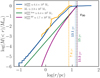 |
Fig. 3 Fraction of dust mass (Mdust, blue line) and stellar mass (M★, orange line) enclosed within a sphere of radius r. Total masses are indicated in the legend. Vertical dashed lines mark the radii containing 90% of the total mass for each component (rdust,90 and r*,90) with values reported in the figure. As a reference, we show the enclosed dust for the S20 model in the homogeneous ( |


3.2 MC absorption properties
We now analyze the absorption properties of the MC at the reference snapshot, by using the dust distribution to compute the cloud optical depth in different bands.
We computed the optical depth directly from the dust distribution in the simulation box with the following method. We randomly drew 100 radial lines of sight (l.o.s.) from the center of the box, which are schematized as cylinders. These lines of sight should not be confused with the detectors’ observing directions described in Sect. 2.2.4. Each cylinder has an axis that starts from the center of the simulation box (a cube with 60 pc side length) and extends for a length of L = 52 pc (corresponding to the diagonal of the box, the maximum distance that can be traversed from the center within the box). The orientation of the axis is chosen by uniformly sampling the solid angle with 100 random unit vectors. Each cylinder was divided into 100 logarithmic spaced radial bins, starting from 0.05 pc (comparable to ∆x = 0.06, the maximum spatial resolution from the D20 simulation), and has a section area of radius rcyl = 2∆x. Each radial bin contributes to the total optical depth, τλ , at a wavelength, λ, by a term:
 (1)
(1)
where Σdust,bin is the dust surface density within the considered bin, κλ is the dust opacity at wavelength λ, and ∆rbin the radial extension of the bin. The dust surface density in the bin was computed by
 (2)
(2)
where Mdust,bin is the total mass of the dust cells with a distance lower than rcyl from the cylinder axis. The contribution of each bin is integrated radially outward from the center so that the dust optical depth at radius r is given by
 (3)
(3)
and the sum runs for all the bins of the cylinder at distances smaller than r from the center of the box. After this computation was performed for all the 100 l.o.s., we computed the median optical depth profile by assigning to each radial bin the median value of the optical depth for that radial bin over the 100 l.o.s. We computed the 16th and 84th percentiles with the same procedure. We underline that the optical depth computed in this way for each line of sight represents the “slab opacity:” the opacity that a source placed in the center would experience along the specific line of sight.
In the top panel of Fig. 4, we show the UV optical depth at 1600 Å (τUV), integrated radially outward, as a function of the cloud radius; τUV has been computed for 100 lines of sight, and the median is shown as a solid line, while the shaded region shows its variance. The median UV optical depth rapidly increases from τUV ~ 10−2 to τUV ~ 1 at r ~ 1 pc, and finally saturates at τUV ~ 30 at ~7.3 pc, a smaller distance than the radius at which 90% of the dust mass is enclosed, rdust,90 ≃ 13.1 pc. The variation in the optical depth between different lines of sight spans 0.5 dex, which is relatively modest considering the later stages of the evolution. In fact, ≈0.3 Myr after the reference snapshot, the cloud morphology becomes even more complex (cf. Appendix A, particular Figs. A.2 and A.3), producing variations of more than 2 dex between different lines of sight at distances of a few parsecs from the center of the cloud.
We also compare the slab optical depth discussed above with the effective opacity, defined as τλ,eff such that  , where Fλ is the detected flux and Fλ,0 the flux that would be received without dust. Here, the fluxes considered are the ones measured by the detectors placed outside the simulated box, as is described in Sect. 2.2.4. This quantity provides an estimate of the radiation that is effectively removed toward the direction pointed by the detector, accounting for the relative distribution between stars and dust, plus RT effects. The effective UV optical depth ranges between τUV,eff = 1.97−4.65 for the six observing directions used for the post-processing RT (see Sect. 2.2.4), with the reference observing direction having τUV,eff = 1.97 (cf. the τUV map in the bottom right panel in Fig. 2). This value implies an overall UV transmission along this direction of
  , consistent with the UV map in Fig. 211. We notice that there is a large difference between the UV optical depth estimated from the dust distribution (τUV ≈ 30) and the effective UV optical depth (τUV,eff ≲ 5). We remind the reader that the former is the slab opacity computed from the cloud center; that is, the optical depth that a source placed in the center of the MC would see toward a radial line of sight. Given that stars are displaced in several positions (cf. Fig. 2), many of them experience little to no dust attenuation toward the direction of the detector. Thus, the dust-to-stellar geometry has a profound impact on the attenuation properties of the MC and on the UV escape fraction.
We compare the optical depth of the simulated MC with the analytical model by S20, for the homogeneous case and the radiation–pressure case. In the first case, it increases from τUV = 0.1 at r ≈ 0.15 pc to τUV ~ 10 at r ≈ 15 pc, as in this model  . Despite the cloud considered in the analytical model having the same mass as the cloud in the simulation, the median optical depth in the simulated MC has a larger value at the cloud boundary with respect to the analytic model, because most lines of sight pass through high-density clumps. In the radiation–pressure model, the inner region of the cloud is significantly dust-deprived by the effect of radiation pressure (cf. Fig. 3). As a result, the UV optical depth remains very low and becomes τUV ≈ 1 only at r ≈ 6 pc. At the cloud boundary, it reaches
  , thus even in this model the cloud is overall UV optically thick. This high value of τUV is consistent with the fact that the dust mass retained by the cloud in this model is ≈73% of the original one. From this comparison, we note that, despite their simple geometric assumptions, both analytical models have some merit in describing the optical depth in the simulated MC. In particular, the RP model provides the best estimate of the effective UV optical depth at the edge of the cloud, whereas the homogeneous model better reproduces the profile of the physical UV optical depth.
In the bottom panel of Fig. 4, we show the IR optical depth. Despite the high-density filaments and clumps, the simulated MC is always optically thin in the IR among all the considered lines of sight, due to the fact that the dust opacity κ100 µm is a factor of ≈2000 lower than κ1600 Å. The IR optical depth has a median value increasing from τIR ~ 10−5 to τIR ~ 1.6 × 10⁻² at the saturation distance of ~5 pc. Even considering the variance between different lines of sight, the IR optical depth stays always below 0.1. Similarly, for the homogeneous model in S20, the IR optical depth increases from  to
to  . Instead, in the radiation-pressure model, the IR optical depth is much lower, analogously to the UV case. At the cloud boundary,
  .
.
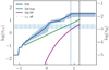 |
Fig. 4 Absorption properties of the MC at the reference snapshot. UV optical depth (τUV at 1600 Å , left y axis) and IR optical depth (τIR, at 100 µm , right y axis) as a function of the cloud radius (r). The optical depths are computed along radial lines of sight from the center of the cloud, as is described in Sect. 3.2. The solid blue line gives the median value over 100 lines of sight, while the shaded region indicates the variance (16th–84th percentiles). The shape of the profiles of the UV and IR optical depths computed from the dust distribution is the same and the two profiles are simply re-scaled due to the different dust opacities in the two regimes: τUV/τIR = κ1600 Å/κ100 µm ≈ 2000. The shaded light blue area brackets the values of the effective optical depth for the six detectors’ observing directions, obtained as |

3.3 Cloud emission
In Fig. 5, we analyze the emission of the reference snapshot, by comparing the intrinsic (e.g., dust-transparent) SED and the dust-obscured SED for the six observing directions used in the RT post-process. The intrinsic emission at 0.1 µm ≲ λ ≲ 1 µm is attenuated up to one order of magnitude for the reference observing direction, which is the least attenuated observing direction. The observed UV emission has a scatter of one order of magnitude, as is also suggested by the estimate of the effective UV optical depth shown in Fig. 4. In terms of the UV slope βUV , defined as
 (4)
(4)
where (λ1,λ2) = (1600,2500) Å, all the observing directions show a negative slope, with −0.5 ≲ βUV ≲ −0.2. The optical- NIR part of the SED shows a flat slope for most of the observing directions; however, the most attenuated ones show an increase toward longer wavelengths. The mid-infrared (MIR) part of the SED is mainly characterized by emission from PAHs at 3.3, 6.2 µm, and 11.2 µm, and by the silicate absorption feature at 9.7 µm. At longer wavelengths, the SED shows the characteristic IR bump corresponding to dust thermal emission, with a peak at λpeak = 80 µm.
As a reference, we also show the results from the analytic model by S20. In the homogeneous case, the IR emission peaks at a shorter wavelength λpeak = 40 µm with respect to the simulated MC. The peak of the IR emission is related to the dust temperature distribution in the cloud. Hence, the difference in the peak wavelength suggests that the dust component in S20 settles on higher temperatures than the simulated reference snapshot. In the homogeneous case, this is caused by the presence of dust in the central region of the cloud, which is directly irradiated by stars without experiencing any shielding effect. We further discuss this point in Sect. 3.4. In the case including radiation pressure, the IR emission peaks at a longer wavelength λpeak = 55 µm with respect to the homogeneous model. This is due to the fact that in this model most of the dust is at a large distance from the center, thus the flux contributing to the dust heating is lower because of geometrical dilution. As a result, the temperature settles to lower values with respect to the homogeneous model (see Sect. 3.4). Moreover, when dust mass is pushed outside and accumulated in an outer shell with a larger volume, the density becomes lower. However, the dust UV optical depth at the cloud boundary is still larger than 1 ( , cf. Fig. 4), therefore the overall IR emission is the same as in the homogeneous model, because of the LTE assumption in the analytic model (e.g., the IR emission is equal to the absorbed UV luminosity).
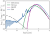 |
Fig. 5 Cloud SED (Lν) for the reference snapshot as a function of wavelength (λ). The solid blue line shows the UV-to-FIR emission of the cloud obtained from the RT post-processed along the reference observing direction. The dashed blue lines correspond to the other five observing directions. The shaded area brackets the fluxes of all the observing directions adopted. The dashed black line indicates the intrinsic (dust-transparent) emission of the cloud along the same observing direction. As a reference, we also show the emission of a local cloud from the analytic model by S20 in the homogeneous case (green line) and in the radiation–pressure case (magenta line). |
3.4 Dust temperature in the cloud
The IR emission of the MC discussed in Sect. 3.3 originates from thermal radiation by dust grains, whose temperature depends on the luminosity of the radiation sources and the distance from them. In Fig. 6, we show the dust temperature radial profile of the MC at the reference snapshot. In particular, we consider for each spherical shell the “mass-weighted” dust temperature, ⟨Td⟩M, and the “luminosity-weighted” dust temperature, ⟨Td⟩L12. The first quantity provides an estimate of the dust temperature of the bulk of the dust component, whereas the second is biased toward the brightest dust grains, likely the ones strongly irradiated by close stars. The median of ⟨Td⟩M is ≈34 K in the innermost region (r < 1 pc) and slowly decreases down to 17 K at the cloud boundary. It shows a very small scatter, suggesting that most of the dust mass spans a limited range in dust temperatures. The median of ⟨Td⟩L follows ⟨Td⟩M in the innermost region. However, it features a few strong peaks up to ≈170 K, with some particularly prominent at 1.6 pc, 3 pc, 4.5 pc, and 7.8 pc. These peaks correspond to spherical shells containing massive stars (m⋆ > 40 M⊙) with a strong radiation field. The position of such massive stars is also emphasized in the figure and it is remarkably consistent with the peaks in the luminosity- weighted profile. Moreover, the smaller the radius, the higher and narrower the ⟨Td⟩L peaks, because of the spherical averaging.
For comparison, we also show the dust temperature obtained from the analytical model by S20, averaged over the mass of dust grains. In the homogeneous model, the dust temperature peaks at ≈200 K in the center and drops toward larger distances. This behavior is expected because, in this model, all the stars are placed in the center of the cloud, and therefore the dust in the innermost region is heated toward high temperatures, whereas at higher distances the flux is reduced because of geometrical dilution and dust attenuation. The high-temperature component in the S20 homogeneous model is responsible for an IR SED which peaks at a shorter wavelength with respect to the simulated MC (cf. Fig. 5). In the radiation–pressure case, the dust temperature shows a very different profile, due to the different spatial distribution. It has a very low value in the central region and then increases going outward as the optical depth increases. It reaches a peak of Td ≈ 80 K at r ≈ 2 pc, and then slowly decreases again as the outer shells experience a higher UV optical depth and therefore receive less flux from the central stars.
We further investigate the dust temperature within the MC by considering the overall temperature distribution instead of the spatial distribution: we show in Fig. 7 the probability distribution functions (PDFs) weighted by mass (light blue) and luminosity (blue) over all the dust cells in the computational box of the RT post-process. The mass-weighted PDF has a narrow distribution, with a median at  , K, where the error bars mark the 16th and 84th percentiles. This estimate indicates a mild skewness toward higher temperatures, due to the presence of the hottest dust cells, which constitute only a small fraction of the total dust mass. As a reference, the total dust mass above 80 K is ≈0.14 M⊙; that is, ≈0.02% of the total dust mass (cf. the right panel in Fig. 8). The hot dust component is well emphasized by the luminosity-weighted PDF, which shows a wide distribution, with multiple peaks at T > 100 K. The median of this distribution is
In the homogeneous model of S20, most of the dust tends to be colder than in the simulated MC, but also in this case a mild skewness toward higher temperature is present, with  This asymmetry in the distribution is driven by the central warm dust regions. The total dust mass above 80 K is 0.46 M⊙ , a factor of 3 higher than in the simulated MC. As a result, also the median of the luminosity-weighted distribution is higher,
  . This is reflected in the FIR emission, which peaks at shorter wavelengths with respect to the simulated MC (cf. Sect. 3.3 and Fig. 5). However, the luminosity- weighted temperature distribution is more compact than in the simulated MC, as there are no extreme regions with dust temperature T > 300 K due to the presence of small pockets of dust very close to a luminous star.
In the radiation–pressure model of S20 the dust temperature covers a much narrower range because it is pushed at a large distance from the center. As a result, the mass-weighted and luminosity-weighted distribution are much similar, with  and
and  , respectively.
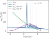 |
Fig. 6 Dust temperature radial profile of the MC at the reference snapshot. The light blue (dark blue) line shows the median of the mass- weighted (luminosity-weighted) dust temperatures in spherical shells; the corresponding shaded areas bracket the 16th–84th percentiles. Vertical dotted lines mark the positions of massive (m⋆ ≥ 40 M⊙) stars. As a reference, we show the temperature profile for the S20 model in the homogeneous case (green line) and in the radiation pressure case (magenta line). |
4 Evolution of MC properties
Having thoughtfully analyzed the reference snapshot, which has been selected at t ≈ 1.1 Myr since the beginning of the SF process, we can now explore the entire evolution. In particular, we investigate the evolution of its emission and absorption properties.
4.1 Dust temperature evolution
We now examine how the evolution of the radiation field and of the dust morphology affects the dust temperature distribution throughout the cloud lifetime.
We use the median values of the mass-weighted and luminosity-weighted distributions (⟨Td⟩M and ⟨Td⟩L , respectively) and their variance as indicators of the dust temperature distributions (cf. Fig. 7). In Fig. 8 we plot the median values of the mass-weighted and luminosity-weighted distributions for the simulated MC and the local cloud analytical models by S20. We find that ⟨Td⟩M and ⟨Td⟩L remain almost constant at ≈20–30 K and 40–50 K, respectively, during the first 1 Myr of the evolution of the cloud, when SF proceeds at a low rate (SFR ≲ 10−2 M⊙ yr−1 ) and the number of very bright stars is low. This is further emphasized by the evolution of the dust mass fraction above a certain temperature Td at different stages of the cloud evolution, shown in the right panel of Fig. 8. At this stage, less than 1% of the total dust mass is heated above 50 K.
After t ≃ 1 Myr, the radiation field increases in intensity, and both ⟨Td⟩M and ⟨Td⟩L start to increase, but their evolution is quite different. The former, tracing the bulk of the dust mass, which is mostly heated by the diffuse radiation, grows mildly up to ≈52 K at t ≃ 1.8 Myr, and then slowly decreases in the later stages of the cloud evolution, when the SFR in the cloud drops because of the cloud photo-ionization. Thus, ⟨Td⟩M mostly follows the evolution of the SFR. Instead, ⟨Td⟩L grows from t ≃ 1 Myr up to the end of the simulation, reaching ≈200 K. This is because the dusty clumps close to bright stars, which are the ones mainly traced by ⟨Td⟩L , keep receiving photons by these already formed stars, whereas the total SFR in the cloud declines. The importance of small, hot clumps in driving the evolution of ⟨Td⟩L can be understood in terms of the cumulative mass fraction above a given temperature. Between 1.0 ≲ t ≲ 1.8 Myr, the fraction of mass above 100 K progressively increases up to ≈25% of the total. After 1.8 Myr, it decreases down to less than 10%; however, this smaller amount of dust above 100 K is heated to higher temperatures. This can be appreciated by the tail in the profile, with an increasing fraction of dust above 150 K as the cloud evolves.
We compare these results from the RT calculations with the predictions from the analytical model by S20 for a local cloud. In the uniform case,  remains constant at 10–20 K up to t ≃ 1.8 Myr, as most of the radiation from the central stars is absorbed by the innermost shells in the cloud and therefore the bulk of the dust mass does not change significantly its temperature. After the peak in the SFR, with the cloud having less dust mass (and thus less attenuation from the inner shells),
  quickly rises up to ≈55 K. On the other hand,
  starts from ≈56 K at the beginning of the cloud life, and moderately rises up to ≈150 K at t ≃ 1.8 Myr, as the inner shells experience more and more radiation. When the SFR begins to drop,
  follows too, reaching ≈137 K at the end of the simulation. In the radiation-pressure case, the
  evolves similarly to the simulated 〈Td〉M up to t ≃ 1.5 Myr. While the radial profiles appear quite different at r ≲ 10 pc (see Fig. 6), this does not affect significantly the average temperature, since only ≈10% of the dust mass is located within this radius (see Fig. 3).
From t ≳ 1.5 Myr, the dust mass loss due to radiation pressure becomes relevant in the analytic model, thus the dust mass retained in the cloud gets heated to higher temperature in the presence of the same radiation field. As a result,  increases to ≈70 K and remains constant after t ≳ 1.8 Myr. On the other hand,
  presents a very mild evolution throughout the cloud lifetime, starting at 40–50 K and slowly growing up to ≈70 K at t ≃ 1.8 Myr. This is a consequence of the fact that radiation pressure pushes the dust away from the central stars so that there are no dust shells that experience a strong radiation field. This is also shown in the detailed spatial distribution (cf. Fig. 6) and in the dust temperature distribution (Fig. 7, right panel). At t ≳ 1.8 Myr
  remains constant at almost the same value as
  , because at this stage the intense radiation pressure has confined most of the dust mass in the outermost shells, which therefore reach very similar temperatures.
This comparison shows that the radiation–pressure model is able to provide a realistic description of the bulk of the dust temperature within the cloud and of its IR emission (cf. Fig. 5), until t ≃ 1.5 Myr; that is, around 0.3 Myr after the moment the cloud is effectively dispersed in this model. However, due to the simplistic stellar-to-dust geometry, it is not able to capture the high-temperature regions, corresponding to clumps irradiated by close bright stars.
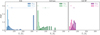 |
Fig. 7 Dust temperature distribution in the MC at the reference MC. The PDFs are weighted by mass and luminosity, with ΔT ≈ 7.1 K and 50 bins. The left panel refers to the simulated MC in D20, the middle panel to the homogeneous model in S20 and the right panel to the radiation–pressure model. Circles indicate the median of each distribution, whereas the dotted lines bracket the 16th and 84th percentiles. |
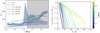 |
Fig. 8 Evolution of the dust temperature during the cloud lifetime, after the onset of SF. Left panel. The solid light blue (dark blue) line shows the median of the mass-weighted (luminosity-weighted) distributions for the simulated MC. The shaded areas mark the 16th and 84th percentiles of each distribution. The light green (dark green) line shows the evolution of the mass-weighted (luminosity-weighted) distributions for the local cloud model by S20 in the uniform case. For the radiation pressure case, we show in light magenta (dark magenta) the mass-weighted (luminosity- weighted) distributions. The shaded gray area highlights the period when the cloud is dispersed according to the radiation–pressure model from S20 (cf. Sect. 2.3.) Right panel. Cumulative distribution of the fractional mass of dust (Md(T > Td)/Md,tot) that has a temperature larger than Td, color-coded according to the evolution time t of the MC. |
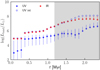 |
Fig. 9 Luminosity evolution for the MC. Total UV (blue) and IR (red) luminosity as a function of cloud age since the onset of SF. Empty circles show the intrinsic stellar radiation, i.e., ignoring dust absorption. Full circles indicate the median luminosity among the different observing directions considered, whereas the error bars bracket the minimum and maximum luminosity. The shaded area highlights the period when the cloud is dispersed according to the radiation–pressure model from S20 (cf. Sect. 2.3). |
4.2 Evolution of the emission properties
In Fig. 9, we show the total radiation emitted from the cloud in the UV (0.1–0.3 µm) and IR (8–1000 µm) bands for the selected snapshots at all the simulated detectors’ observing directions, emphasizing the median values. The UV radiation produced by stars (empty blue circles) increases throughout the MC evolution loosely following the average trend of the SF history (cf. Fig. 1). At t ≲ 0.3 Myr, the intrinsic emission is ~105 L⊙, of which only ≈1% survives dust attenuation along the median observing direction. At this stage, the cloud UV emission also shows a strong dependence with the observing direction, with variations of almost three orders of magnitude; this behavior is caused by the fact that at this stage only a few stars (≈70, with a total mass of M★ ≈ 170 M⊙) are in place, making geometric effects very important for the dust attenuation. At t ~ 0.3 Myr, the cloud emission increases by around one order of magnitude both in the UV and IR. This is due to the birth of a star with M★ > 40 M⊙, which significantly boosts the photon production ( ). After this episode, the overall luminosity remains broadly constant in both the UV and IR bands up to t ~ 1 Myr, and also the dependence of the UV emission with the observing direction is significantly reduced. Moreover, during this stage up to t ~ 1.5 Myr, the IR emission is almost equal to the intrinsic UV emission; that is, LUV ≃ LIR. After this point, the intrinsic UV emission increases again, reaching 3.7 × 10⁷ L⊙ at t ≃ 1.7 Myr, when the cloud begins to photo-evaporate. However, during this period, the dust-attenuated UV luminosity does not increase with the same pace, and actually decreases after t ≃ 1.4 Myr, suggesting an increase in the effective optical depth for the whole MC. Between 1.3 ≲ t ≲ 1.5 Myr, the MC showcases a slightly higher IR luminosity with respect to the intrinsic UV luminosity. This is a consequence of the increased intrinsic emission outside the range 0.3–1.0 µm, whose contribution to the dust heating becomes significant, see also footnote 10. In the latest stages (t > 1.7 Myr), the SFR in the simulated MC flattens and then starts to drop; however, the UV intrinsic stays constant, because massive stars are still seeded. Instead, the UV emission steadily increases among all observing directions, as a result of an increased UV escape fraction, due to the cloud photo-evaporation (see later on in Fig. 12). We also notice that during this epoch the IR emission is a factor of ≈2 lower than the UV intrinsic luminosity, whereas they were almost comparable before t ~ 1.5 Myr. This is due to the scattered light outside the observing direction, as can be seen by the error bars of the UV and FIR in Fig. 9.
We further study the evolution of the emission by considering the whole SED. In Fig. 10, we show the SED of the MC at each of the selected snapshots, normalized to the SFR of the snapshot, and color-coded based on the time after the beginning of SF. For this comparison, we discuss only the evolution of the SEDs relative to the reference observing direction. Overall, the SEDs show a similar shape throughout the evolution, with the total luminosity that increases as the cloud evolves. However, by inspecting closely each band, a few significant trends emerge. The UV emission increases up to t ≃ 1.5 Myr, then decreases for a short period up to t ≃ 1.8 Myr, and then quickly rises again, as in Fig. 9. The UV SED presents a large variety of slopes ßUV (Eq. (4)): at t ≲ 0.3 Myr, the MC shows positive slopes, ßUV ≃ 0.5; at 0.3 ≲ t ≲ 1.2 Myr it is mainly characterized by mild negative slopes ßUV ≃ −0.5; after t ≲ 1.2 Myr, the slopes tend to flatten up to t ≃ 1.8 Myr, when they decrease again down to ßUV ≃ −0.5. We further discuss the evolution of ßUV, accounting also for the dependence on the observing direction, in Sect. 4.4. In the 1 µm ≲ λ ≲ 10 µm range, the shape of the SED is remarkably similar at each time frame and simply changes in magnitude. They all show the PAHs features at 3.3 and 6.2 µm, and the silicate feature at 9.7 µm. The only exception to this trend is at t ≲ 0.3 Myr, when the SEDs show a flatter slope in this wavelength range. At λ ≳ 10 µm, the PAH features become less and less prominent as the MC evolves, because the dust temperature distribution shifts toward higher values (see Fig. 8), raising the underlying continuum flux.
Finally, the peak of FIR emission increases in magnitude by ~3 orders of magnitude throughout the MC evolution, but the wavelength of the peak also shifts toward shorter wavelengths, from 110 µm at t ≈ 0.3 Myr to 31 µm at t ≈ 2.3 Myr. This is due to the shift of the dust temperature distribution toward higher values as the MC evolves because the intensity of the radiation field increases as more and more stars are seeded (cf. the intrinsic UV emission in Fig. 9).
We compare our results with the RT simulations by JD23, plotting our SEDs against the ones they obtain for the six snapshots analyzed from the simulations presented in Zamora-Avilés et al. (2019). We show the JD23 results for the two observing directions they adopt; namely, the “face-on” view and the “edge- on” one. Our simulated SEDs at t ≲ 1 Myr tend to have lower luminosities (normalized with the SFR) in the UV band with respect to the ones by JD23, with the exception of their snapshots at t = 0.8 Myr and t = 1.6 Myr. At t ≳ 1 Myr the simulated SEDs between the two works span a comparable range in SFR- normalized luminosity. In the MIR range, the SEDs from both simulations are fairly consistent. Instead, in the FIR band, the SEDs by JD23 peak at longer wavelengths with respect to our simulated SEDs. This is due to the fact that the dust component settles to lower temperatures in JD23 with respect to our MC. We attribute this difference to the higher SFE in the simulation considered in this work. In fact, at t ≳ 1 Myr our simulated MC has a SFR 1–2 orders of magnitude higher with respect to the typical values in the simulation from JD23. As a result, the M*/Mgas ratio is at least a factor 4–5 higher throughout the evolution of the cloud. The lower dust-to-stellar ratio results in higher dust temperature in our simulated cloud.
We also compare our results with the photometric data of 28 massive star-forming HII regions in the MW by Binder & Povich (2018). These clouds have an IR luminosity between 4 × 10⁴ L⊙ and 2.3 × 10⁷ L⊙ and they have a SFR (inferred from the IR luminosity) spanning the range 1.8 × 10⁻⁵ M⊙ yr−1 ≲ SFR ≲ 10−2M⊙ yr−1. Therefore, they can be compared to our simulated SEDs up to the reference snapshot at t ≈ 1.1 Myr.
The observed HII regions are quite consistent with the MIR flux from our simulations. However, the FIR data shows a FIR peak at longer wavelengths, suggesting that the simulations are missing a lower dust temperature component. If considering the overall IR emission, the disagreement with observations is milder. In fact, the simulated MC has an IR luminosity of LIR ≈ 106−3 × 10⁷ for most of its lifetime, and the majority (17 out 28) of the clouds in Binder & Povich (2018) have LIR ≈ 106−2 × 10⁷. We attribute the discrepancy between our synthetic SEDs and observations of local HII regions to the SF in our simulated MC. In other words, the intense SF (and feedback) in the MC from D20 depletes the gas and therefore the dust component, which is then heated by UV radiation at temperatures that are higher with respect to the observations from the Binder & Povich (2018) sample. This effect might be due to the absence of magnetic fields and to the lack of full turbulence driving in the D20 setup. Indeed, both factors can contribute to preventing gravitational collapse, in turn reducing the SFE, and thus the depletion.
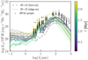 |
Fig. 10 Evolution of the MC SED as a function of wavelength, normalized to the SFR. Each line corresponds to a different evolution time t of the MC, as is shown in the color bar. For the sake of clarity, at each t we show only the SED for the reference observing direction. Dashed gray lines show the results of the RT simulations by JD23 for their snapshots from 0.8 Myr to 7.5 Myr for their face-on view (dashed lines) and edge-on view (dotted lines). Black points indicate the photometric data relative to the 28 active clouds analyzed in Binder & Povich (2018). |
4.3 Evolution of dust attenuation properties
In Fig. 11, we show the attenuation properties of the MC throughout its evolution. The attenuation, Aλ, is defined as
 (5)
(5)
where  and
and  are the observed and intrinsic flux at the wavelength, λ, respectively. We first focus on a single wavelength, by studying A3000, the attenuation at 3000 Å, which is often used to pinpoint the attenuation curves. The left panel of Fig. 11 shows A3000 as a function of the cloud age. At the beginning, the median attenuation is A3000 ≈ 4, with a large scatter among different observing directions. Then, at t ~ 0.4 Myr, it drops to A3000 ≈ 2, and the scatter between different observing directions is progressively reduced as the cloud evolves and the number of stars formed increases. From t ~ 0.4 Myr onward, the median attenuation keeps increasing during the cloud evolution up to A3000 ≈ 5 at t ~ 1.8 Myr (when the volume occupied by HI reaches a peak, cf. Fig. 9 in D20). After this period, the cumulative effect of stellar feedback leads to cloud photo-evaporation, with the formation of many cavities and a dust loss of a factor 2 since the beginning of SF. As a result, A3000 drops steadily down to ≈3 at the end of the simulation.
In the right panel of Fig. 11, we show the attenuation curve, normalized to A3000 , at the same snapshots as in the left panel. For each snapshot, we plot only the observing direction with the median value of A3000. This choice allows us to not be biased toward a specific direction at certain times, and to provide a description of the average attenuation properties of the MC. However, we underline that a single observing direction does not provide the full picture of the variety of the attenuation curves in the MC.
Immediately after the onset of the SF the attenuation curve is close to the Milky-Way extinction curve, with a slightly less pronounced bump at 2175 Å, and a less steep rise at short wavelengths. In the time period between 0.4 ≲ t ≲ 1 Myr, the attenuation curve experiences a rapid variation: the bump is suppressed for a short time, then it reappears almost as strongly as at the beginning and then it is suppressed again. At short wavelengths, the curve remains flatter than the original Milky-Way extinction and becomes closer to the attenuation curve obtained by Calzetti et al. (2000) for a sample of low-redshift starburst galaxies (hereafter the “Calzetti curve”). After t ~ 1 Myr, the bump strength slowly increases, with some variation at different times, whereas the slope of the curve becomes flatter than the Calzetti curve.
We do not find a clear correlation between the strength of the 2175 Å -bump and the attenuation A3000 nor between the steepness of the attenuation curve and A3000. We instead find a mild correlation with the relative variation in A3000 across the observing directions, defined as  . This suggests that geometry effects (e.g., the spatial distribution of dust and stars and the observing direction considered) play a major role in shaping the attenuation curve in the simulated MC.
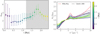 |
Fig. 11 Evolution of the MC attenuation. Left panel: flux attenuation at 3000 Å at different times during the cloud evolution. The circles indicate the median A3000 among the considered observing directions, whereas the error bars bracket the minimum and maximum values. The shaded area highlights the period when the cloud is dispersed according to the radiation–pressure model from S20 (cf. Sect. 2.3). Right panel: flux attenuation (normalized to the attenuation at 3000 Å) as a function of the inverse of the wavelength for the post-processed snapshots. The attenuation curves are shown only for the observing direction with the median value of A3000 at each snapshot. Dashed lines show the extinction curve for the MW (red) and the attenuation curve found by Calzetti et al. (2000, black). |
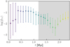 |
Fig. 12 Evolution of the UV (0.1–0.3 µm) escape fraction for the simulated MC. Filled circles indicate the median escape fraction among the different observing directions, whereas error bars bracket the minimum and maximum escape fractions. The shaded area highlights the period when the cloud is dispersed according to the radiation–pressure model from S20 (cf. Sect. 2.3). |
4.4 Main UV and IR emission diagnostics
We further investigate the cloud emission properties, by studying how much radiation in the UV band effectively escapes the cloud. In Fig. 12, we show the evolution of the UV escape fraction fUV = LUV/LUV,int. In the first ~0.3 Myr after the beginning of SF, fUV shows a variability of three orders of magnitude with the observing direction, spanning a range from 10–3 to 10–1, with a median value of 10–2. This large scatter is mainly due to the variance associated with the low number of stars in place at this stage. At t ~ 0.3 Myr, the UV escape fraction increases by an order of magnitude with a median value of fUV ≈ 10–1. This increase happens together with the rise in the UV intrinsic luminosity (cf. Fig. 9), suggesting that it is associated with newly born stars that experience an average lower attenuation. The higher number of stars also reduces the scatter in fUV to 1.5 dex. The UV escape fraction remains constant up t ≈ 1 Myr, then it decreases slowly up to t ≈ 1.5 Myr, with also a lower scatter between distinct observing directions. Between 1.5 ≲ t ≲ 1.8 Myr, it drops quickly to 3 × 10⁻³ and also the variation between observing directions increases. At t ≳ 1.8 Myr, the cloud begins to photo-evaporate, and this is clearly reflected in the increase in the UV escape fraction, which rises up to 3 × 10⁻² at the end of the simulation, when ≈ 1/3 of the initial gas (and dust) mass is retained. Meanwhile, the scatter between different observing directions is reduced, as most of the SF is concentrated in the center and geometry effects play a minor role (cf. Fig. A.3).
In the context of galaxy evolution, an important diagnostic tool to quantify the conversion of UV photons into dust thermal emission in the IR band is the IRX-β relation, which describes the IR excess IRX ≡ LIR/LUV as a function of the UV slope βUV (see Eq. (4)). In Fig. 13, we show the IRX-β relation for the simulated MC at different times for each of the observing directions considered in the RT post-process. The MC occupies a wide range of positions in the IRX-β diagram, with –0.5 ≲ βUV ≲ 2 and 0 ≲ log(IRX) ≲ 3.5. In most cases, the MC appears with a –0.5 < βUV < 0 and 0.5 < log(IRX) < 2. Interestingly, the position in phase space of the MC at similar times (or even at the same age) changes dramatically depending on the observing direction, in particular at early stages (t ≲ 0.5 Myr). Instead, after the cloud starts to disperse (t ≳ 1.8 Myr) it settles at –0.5 < βUV < 0 and log(IRX) = 1. We compare our results with local observations collected in Calzetti et al. (2021), in particular a sample of local starburst galaxies (Calzetti et al. 1994; Meurer et al. 1999), nearby star-forming galaxies (Dale et al. 2009) and individual star-forming regions in the local galaxy M51 (Calzetti et al. 2005). We also show together with the individual data the empirical fitting relations obtained by Meurer et al. (1999) (see also Overzier et al. 2011; Takeuchi et al. 2012 for the revised relations with aperture-corrected data) and Calzetti et al. (2000) for their starbursts samples, and the relation from Casey et al. (2014), derived for a sample of local galaxies. We find that most observations have βUV < –0.5, smaller than all the values of our simulated MC, thus suggesting lower dust attenuation of their intrinsic emission. Many IRX-β points of the simulated MC at early and intermediate times (t ≲ 1.7 Myr) are consistent with the empirical relations, either of starbursts galaxies or of starforming galaxies. Some points lie above the starbursts relation by Calzetti et al. (2000), but they are consistent with the scatter from the individual galaxies. Around half of the points of the simulated MC lie below the relation of star-forming galaxies, in particular after the cloud becomes dispersed. It is interesting to note that many of these points are still in agreement with the measurements of individual regions in the local galaxy M51 (Calzetti et al. 2005). Overall the observed galaxies and individual regions show a scatter in the IRX-β plane that is not dissimilar to the scatter of the simulated MC throughout its evolution. Moreover, this comparison emphasizes how the evolutionary stage of a single MC can affect its position in the IRX-β diagram. Given that the emission of a galaxy contains the contribution of MCs that are at different evolutionary stages, such as obscured MCs and dispersed MCs, altogether, we caution toward the interpretation of the evolutionary stage of an entire galaxy based on its integrated IRX-β diagram.
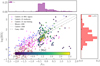 |
Fig. 13 IRX-β relation during the evolution of the MC. For each snapshot, we computed the IRX-β values for each observing direction. We show all of them as circles, color-coded according to the time since the onset of SF. The upper and right insets show the 1-D PDF of βUV and IRX, respectively. We also show the data collected in Calzetti et al. (2021) relative to local starburst galaxies (Calzetti et al. 1994; Meurer et al. 1999, blue stars), nearby star-forming galaxies (Dale et al. 2009, brown circles) and individual star-forming regions in the local galaxy M51 (Calzetti et al. 2005, magenta triangles). We also show with gray lines the empirical fitting relations obtained by Meurer et al. (1999) and Calzetti et al. (2000) for their starbursts samples, and the relation from Casey et al. (2014) for local galaxies. |
5 Summary and conclusions
In this work, we have presented Monte Carlo RT calculations with the code SKIRT (Camps & Baes 2015, 2020) performed to post-process the RHD simulation from D20, which follows the evolution of a local MC with gas mass of Mgas ≈ 105 M⊙ down to a spatial resolution of 0.06 pc. We have investigated the physical properties (e.g., cloud morphology, dust absorption, dust temperature) and multiwavelength emission properties (e.g., SED, UV escape fraction, attenuation curve) using the essential, physically motivated MC emission models from S20 as a baseline benchmark, in particularly adopting the “homogeneous” dust distribution and “radiation pressure” models as bracketing cases. This work represents a starting point toward the development of sub-grid prescriptions to describe the structure and emission of unresolved structures in cosmological hydrodynamic simulations of galaxy formation. We also tested our results against similar works from the literature and observations of local MCs.
At the reference snapshot (t ≃ 1.1 Myr after the beginning of SF), the cloud shows a very complex morphology, with filaments and clumps, but also low-density channels cleared out by stellar feedback (Fig. 2). At this stage, it has a dust mass of Mdust = 6.4 × 10² M⊙, a stellar mass of M★ ~ 2.3 × 10³ M⊙, and a SFR of SFR ~ 0.01 M⊙ yr–1.
The UV optical depth derived from the dust distribution, computed along radial lines of sight from the center to the edge of the MC, has a median value of τUV ~ 30, with a 0.5 dex variation between different lines of sight. However, the presence of low-density channels and the intermixed distribution between dust and stars result in an effective UV optical depth between τUV,eff = 2.0–4.6 for different observing directions (Fig. 4, top panel). As a result, dust attenuation suppresses ≳90% of the UV flux emitted by stars at this stage, with a scatter of one order of magnitude in emission depending on the observing direction. We find the homogeneous model by S20 to better reproduce the radial profile of the UV optical depth, whereas the RP model provides the best estimate of the effective UV optical depth at the edge of the cloud ( ). The MC at the reference snapshot is always optically thin (τIR < 0.1) in the IR among all the considered lines of sight from the center, both in the simulation and analytical models (Fig. 4, bottom panel).
The IR emission in the three models peaks at different wavelengths (λpeak = 80 µm in the simulation, λpeak = 40 µm in the homogeneous model and λpeak = 55 µm in the radiation pressure model, Fig. 5), reflecting the different dust temperature distributions in the three models (Fig. 7). The simulated cloud has a bulk component at T ≈ 26 K, but also multiple peaks at T > 100 K, corresponding to small pockets of dust very close to a luminous star (Fig. 6). In the S20 homogeneous model, central regions reach temperatures T ≈ 200 K, as they are directly irradiated by stars without experiencing any shield effect, whereas in the radiation–pressure model the temperatures are lower because of the geometrical dilution due to most of the dust being pushed at large distances from the center.
Throughout the cloud evolution, the emission changes significantly as a result of the complex evolution of its absorption properties and its SF history. The UV (0.1–0.3 µm) radiation produced by stars loosely follows the average trend of the SFR up to the cloud photo-evaporation, growing from ~105 L⊙ to 3.7 × 10⁷ L⊙ (Fig. 9). At the early stages (t ≲ 0.3 Myr), only a small fraction of this UV emission (fUV ≈ 0.1–10%) survives dust attenuation, with strong variations between different observing directions. Then, the UV transmission increases by one order of magnitude (fUV ≈ 10%) and slowly decreases down to fUV ≈ 0.3% at the cloud photo-evaporation at t ≃ 1.7 Myr, after which several dust-free channels are open, leaving UV radiation free to escape, fUV ≈ 3% (Fig. 12).
The IR (8–1000 µm) emission increases in magnitude by ~3 orders of magnitude throughout the MC evolution, and the wavelength of the peak shifts toward shorter wavelengths, from 110 µm at t ≈ 0.3 Myr to 31 µm at t ≈ 2.3 Myr (Fig. 10). This is due to the shift of the dust temperature distribution toward higher values as the MC evolves (Fig. 8), because the intensity of the radiation field increases as more and more stars are seeded.
The MC position on the IRX-β diagram changes significantly throughout its evolution, strongly depending on the observing direction considered and it moves significantly even after short time variation. After the cloud photo-evaporation, it settles at –0.5 < βUV < 0 and log(IRX) ≃ 1 (Fig. 13). This finding suggests caution in interpreting the IRX-β on the galaxy scale, as different regions would be expected to lie in different locations on the IRX-β plane depending on the local SF stage and observing angle.
In summary, the comparison between the simulated MC and the analytical models in terms of dust temperature distribution (e.g., ⟨Td⟩M, ⟨Td⟩L) and cloud emission (fUV, LIR, SED shape) prefers the inclusion of a mechanical feedback mechanism affecting the gas and dust spatial distribution (in our specific case, the radiation pressure) in order to provide a description closer to the simulations. However, the considered radiation– pressure model is not able to capture the high-temperature regions and it underestimates the cloud dispersal time because all the stars are assumed to be at the center. Moreover, it does not predict a UV escape fraction, as no dust-free channels are present due to the spherical symmetry. A more sophisticated numerical setup, able to predict high-temperature regions irradiated by bright stars, and handling a more complex geometry, would provide more realistic estimates of the relevant physical quantities in describing the cloud emission on sub-grid scales; for example, ⟨Td⟩M , ⟨Td⟩L , fUV, LIR.
Finally, we also compared the results from our simulations to photometric data of 28 massive star-forming HII regions in the MW from Binder & Povich (2018), finding that our SEDs present a FIR peak at shorter wavelengths, despite having comparable IR luminosities (Fig. 10). We attribute the discrepancy to the lack of a cold dust component in our simulations due to an excessive SFE. We plan to refine in the future the adopted SF recipe and to also include the impact of magnetic fields, which we expect would reduce gas consumption and produce MCs with physical conditions similar to the local ones.
Data availability
The derived data generated in this research will be shared on reasonable request to the corresponding author.
Acknowledgements
The authors thank the anonymous referee for carefully reading the manuscript and for the useful comments, which improved the quality of the work and the clarity of the manuscript. We acknowledge usage of the Python programming language (Van Rossum & de Boer 1991; Van Rossum & Drake 2009), Astropy (Astropy Collaboration 2013), Cython (Behnel et al. 2011), Matplotlib (Hunter 2007), NumPy (van der Walt et al. 2011), Numba (Lam et al. 2015), PYNBODY (Pontzen et al. 2013), and, SciPy (Virtanen et al. 2020). We gratefully acknowledge the computational resources of the Center for High Performance Computing (CHPC) at Scuola Normale Superiore, Pisa (IT).
Appendix A Cloud morphology at early and late times
In Sect. 3.1 we discuss the morphology of the MC after t ≃ 1.1 Myr since the beginning of the SF process. To qualitatively illustrate the sensitivity of the cloud morphology due to the evolutionary stage, we report the same physical quantities as in Fig. 2 at three different epochs: i) t ~ 0.5 Myr (Fig. A.1), when ~0.7% of the total final stellar mass is present, ii) t ~ 1.4 Myr (Fig. A.2) when ~3.1% of the total final stellar mass is present, and iii) t ~ 2 Myr (Fig. A.3), when the cloud is toward the end of its life and 36% of the gas mass remains.
Appendix B Convergence of the dust temperature distribution
In this section we discuss the validity of the number of photon packets adopted (5 × 10⁶) in the RT simulations presented in this work. This is of uttermost importance, as an insufficient number of photon packets per source would result in a non-convergent dust temperature close to these sources. This would, in turn, affect the overall dust temperature distribution (Figs. 7, Fig. 8, right panel), and therefore our conclusions regarding in particular the dust temperature profiles (Fig. 6), its variation with the observing direction, and the evolution of the weighted dust temperature distributions (Fig. 8, left panel).
To address this point, we re-simulated the reference snapshot with a number of packets ten times smaller and ten times higher, and we compared the results of these two simulations with the one presented in this work.
In Fig. B.1, we show the results of this comparison in terms of the dust temperature PDF. In the mass-weighted PDF, we notice a small difference in the temperature distribution at Td < 40 K, in particular an excess of mass in the lowest-mass bin in the run with 5 × 10⁵ packets with respect to the other two. The difference between the original run (5 × 10⁶ packets) and the high-resolution run (5 × 10⁷ packets) is instead marginal. Similarly, in the luminosity-weighted PDF, the temperature distribution differs at Td < 50 K in the run with 5 × 10⁵ packets, whereas it is almost identical in the other two runs. This behavior is further strengthened by the summary statistics of the distributions, which are reported in Table B.1. The differences in the median, 16th, and 84th percentiles between the run we analyzed in this work and the one with ten times more photon packets is less than 1 K.
Given that the analysis of the PDF of the dust temperature distribution involves every resolution element of the dust distribution in the RT computation, the convergence of the dust temperature PDF implies the convergence of the integrated quantities related to the dust temperature; for example, the dust temperature profile and the cumulative dust mass distribution. Thus, we conclude that the number of photon packets used in this work is sufficient to achieve the convergence of the dust temperature distribution.
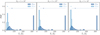 |
Fig. B.1 Probability distribution functions (PDFs) for the reference snapshot of the MC simulation. The PDFs are weighted by mass (light blue) and luminosity (blue). Each panel refers to the same snapshot at t ~ 1.1 Myr (the reference snapshot), simulated with 5 × 10⁵ (left panel), 5 × 10⁶ (middle panel), 5 × 10⁷ (right panel) photon packets. Circles indicate the median of each distribution, whereas the dotted lines bracket the 16th and 84th percentiles. |
Summary statistics of the convergence tests relative to dust temperature distribution.
Appendix C Convergence of the spectral energy distribution
In this section we discuss the reliability of the SED produced by our RT computations, by using the statistics diagnostics introduced in SKIRT in Camps & Baes (2018), based on the work done in the field of Monte Carlo nuclear particles transport (e.g., X-5 Monte Carlo Team 2003). Individual photon packets carry a contribution wi to the flux recorded by a detector in a given bin so that the total contribution to a detector bin would be Σiwi, where the sum runs over the total number N of photon packets launched. For each detector bin, SKIRT records the sums  , for k = 0, 1, 2, 3, 4. The higher-order sums can be used to estimate the relative error R:
 (C.1)
(C.1)
and the variance of variance (VOV):
 (C.2)
(C.2)
The relative error, R, should be smaller than 0.1 for the results to be considered reliable; results are questionable for 0.1 < R < 0.2 and unreliable for R > 0.2. The quantity VOV measures the statistical uncertainty of the value of R, and it should also be smaller than 0.1 to provide a reasonable confidence interval for the relative error R.
We first apply these diagnostics to the SED obtained for the reference snapshot, by also examining how the accuracy of our results changes by increasing the number of photon packets. In Fig. C.1, we show the SED statistics in terms of R and VOV for the reference snapshot. The fiducial run performed with 5 × 10⁶ packets always has R < 0.1 for each observing direction and in each wavelength bin. The same is true for the VOV. We conclude that the number of photon packets used is already sufficient to provide reliable SED predictions for the reference snapshot. Nevertheless, we notice that the statistics improve by a factor of ≈3 both in terms of R and VOV when increasing the number of photon packets by a factor of 10.
We repeat this analysis for every snapshot analyzed in this work. We show the results for every snapshot and every observing direction used in each simulation in Fig. C.2. We find R < 0.1 in almost every case, except for a select number of recorded SEDs that exceed this limit only for a couple of wavelength bins. Similarly, the VOV is in most cases below 0.1 and exceeds the limit just on a few occasions and for a very small portion of the spectrum. We argue that this study shows that the SEDs studied in this work are statistically reliable and so are the corresponding derived quantities (e.g., LUV, LIR, fUV and the IRX -β relation).
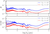 |
Fig. C.1 SED statistics for the reference snapshot. The top panel shows the relative error R, the lower panel shows the variance of variance VOV. Blue (red) lines represent the run with 5 × 10⁶ (5 × 10⁷) photon packets, with each line referring to a different observing direction. The dashed lines in both panels indicate the threshold of 0.1 below which the results are reliable. |
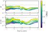 |
Fig. C.2 SED statistics for each snapshot analyzed in this work. The top panel shows the relative error R, and the lower panel the variance of variance VOV. For every snapshot, we show the results relative to the SED of the 6 observing directions, and we color-code the lines relative to each snapshot according to the corresponding time since the beginning of the SF in the MC. The dashed lines in both panels indicate the threshold of 0.1 below which the results are reliable. |
References
- Ali, A. A. 2021, MNRAS, 501, 4136 [NASA ADS] [CrossRef] [Google Scholar]
- Astropy Collaboration (Robitaille, T. P., et al.) 2013, A&A, 558, A33 [NASA ADS] [CrossRef] [EDP Sciences] [Google Scholar]
- Aubert, D., & Teyssier, R. 2008, MNRAS, 387, 295 [NASA ADS] [CrossRef] [Google Scholar]
- Behnel, S., Bradshaw, R., Citro, C., et al. 2011, Comput. Sci. Eng., 13, 31 [Google Scholar]
- Behrens, C., Pallottini, A., Ferrara, A., Gallerani, S., & Vallini, L. 2018, MNRAS, 477, 552 [NASA ADS] [CrossRef] [Google Scholar]
- Binder, B. A., & Povich, M. S. 2018, ApJ, 864, 136 [CrossRef] [Google Scholar]
- Bisbas, T. G., Wünsch, R., Whitworth, A. P., Hubber, D. A., & Walch, S. 2011, ApJ, 736, 142 [Google Scholar]
- Bovino, S., Grassi, T., Capelo, P. R., Schleicher, D. R. G., & Banerjee, R. 2016, A&A, 590, A15 [NASA ADS] [CrossRef] [EDP Sciences] [Google Scholar]
- Bressan, A., Marigo, P., Girardi, L., et al. 2012, MNRAS, 427, 127 [NASA ADS] [CrossRef] [Google Scholar]
- Brunt, C. M., Heyer, M. H., & Mac Low, M. M. 2009, A&A, 504, 883 [NASA ADS] [CrossRef] [EDP Sciences] [Google Scholar]
- Butler, M. J., Tan, J. C., & Van Loo, S. 2015, ApJ, 805, 1 [NASA ADS] [CrossRef] [Google Scholar]
- Calzetti, D., Kinney, A. L., & Storchi-Bergmann, T. 1994, ApJ, 429, 582 [Google Scholar]
- Calzetti, D., Armus, L., Bohlin, R. C., et al. 2000, ApJ, 533, 682 [NASA ADS] [CrossRef] [Google Scholar]
- Calzetti, D., Kennicutt, R. C. J., Bianchi, L., et al. 2005, ApJ, 633, 871 [NASA ADS] [CrossRef] [Google Scholar]
- Calzetti, D., Battisti, A. J., Shivaei, I., et al. 2021, ApJ, 913, 37 [CrossRef] [Google Scholar]
- Camps, P., & Baes, M. 2015, Astron. Comput., 9, 20 [Google Scholar]
- Camps, P., & Baes, M. 2018, ApJ, 861, 80 [NASA ADS] [CrossRef] [Google Scholar]
- Camps, P., & Baes, M. 2020, Astron. Comput., 31, 100381 [NASA ADS] [CrossRef] [Google Scholar]
- Camps, P., Trayford, J. W., Baes, M., et al. 2016, MNRAS, 462, 1057 [CrossRef] [Google Scholar]
- Casey, C. M., Scoville, N. Z., Sanders, D. B., et al. 2014, ApJ, 796, 95 [NASA ADS] [CrossRef] [Google Scholar]
- Castelli, F., & Kurucz, R. L. 2003, in Modelling of Stellar Atmospheres, 210, eds. N. Piskunov, W. W. Weiss, & D. F. Gray, A20 [NASA ADS] [Google Scholar]
- Castor, J. I., Abbott, D. C., & Klein, R. I. 1975, ApJ, 195, 157 [Google Scholar]
- Cen, R. 1992, ApJS, 78, 341 [NASA ADS] [CrossRef] [Google Scholar]
- Ceverino, D., Glover, S. C. O., & Klessen, R. S. 2017, MNRAS, 470, 2791 [NASA ADS] [CrossRef] [Google Scholar]
- Chevance, M., Kruijssen, J. M. D., Hygate, A. P. S., et al. 2020, MNRAS, 493, 2872 [NASA ADS] [CrossRef] [Google Scholar]
- Churchwell, E., Babler, B. L., Meade, M. R., et al. 2009, Publ. Astr. Soc. Pac., 121, 213 [NASA ADS] [CrossRef] [Google Scholar]
- Cochrane, R. K., Hayward, C. C., Anglés-Alcázar, D., et al. 2019, MNRAS, 488, 1779 [NASA ADS] [CrossRef] [Google Scholar]
- Colombo, D., Hughes, A., Schinnerer, E., et al. 2014, ApJ, 784, 3 [NASA ADS] [CrossRef] [Google Scholar]
- Dale, J. E., Bonnell, I. A., Clarke, C. J., & Bate, M. R. 2005, MNRAS, 358, 291 [CrossRef] [Google Scholar]
- Dale, D. A., Cohen, S. A., Johnson, L. C., et al. 2009, ApJ, 703, 517 [Google Scholar]
- Decataldo, D., Pallottini, A., Ferrara, A., Vallini, L., & Gallerani, S. 2019, MNRAS, 487, 3377 [Google Scholar]
- Decataldo, D., Lupi, A., Ferrara, A., Pallottini, A., & Fumagalli, M. 2020, MNRAS, 497, 4718 [NASA ADS] [CrossRef] [Google Scholar]
- Deparis, N., Aubert, D., Ocvirk, P., Chardin, J., & Lewis, J. 2019, A&A, 622, A142 [NASA ADS] [CrossRef] [EDP Sciences] [Google Scholar]
- Di Mascia, F., Gallerani, S., Behrens, C., et al. 2021, MNRAS, 503, 2349 [NASA ADS] [CrossRef] [Google Scholar]
- Di Mascia, F., Carniani, S., Gallerani, S., et al. 2023, MNRAS, 518, 3667 [Google Scholar]
- Dobbs, C. L. 2015, MNRAS, 447, 3390 [CrossRef] [Google Scholar]
- Draine, B. T. 2011, ApJ, 732, 100 [NASA ADS] [CrossRef] [Google Scholar]
- Evans, I., Neal J., Dunham, M. M., Jørgensen, J. K., et al. 2009, ApJS, 181, 321 [NASA ADS] [CrossRef] [Google Scholar]
- Federrath, C., & Klessen, R. S. 2012, ApJ, 761, 156 [Google Scholar]
- Feng, Y., Di-Matteo, T., Croft, R. A., et al. 2016, MNRAS, 455, 2778 [NASA ADS] [CrossRef] [Google Scholar]
- Ferland, G. J., Korista, K. T., Verner, D. A., et al. 1998, Publ. Astr. Soc. Pac., 110, 761 [NASA ADS] [CrossRef] [Google Scholar]
- Forbrich, J., Lada, C. J., Muench, A. A., Alves, J., & Lombardi, M. 2009, ApJ, 704, 292 [NASA ADS] [CrossRef] [Google Scholar]
- Furlanetto, S. R., & Mirocha, J. 2022, MNRAS, 511, 3895 [NASA ADS] [CrossRef] [Google Scholar]
- García, P., Bronfman, L., Nyman, L.-A., Dame, T. M., & Luna, A. 2014, ApJS, 212, 2 [CrossRef] [Google Scholar]
- Gatto, A., Walch, S., Naab, T., et al. 2017, MNRAS, 466, 1903 [NASA ADS] [CrossRef] [Google Scholar]
- Geen, S., Bieri, R., Rosdahl, J., & de Koter, A. 2021, MNRAS, 501, 1352 [Google Scholar]
- Glover, S. C. O., & Abel, T. 2008, MNRAS, 388, 1627 [NASA ADS] [CrossRef] [Google Scholar]
- Grassi, T., Bovino, S., Schleicher, D. R. G., et al. 2014, MNRAS, 439, 2386 [Google Scholar]
- Guillet, T., & Teyssier, R. 2011, J. Computat. Phys., 230, 4756 [NASA ADS] [CrossRef] [Google Scholar]
- Haid, S., Walch, S., Seifried, D., et al. 2018, MNRAS, 478, 4799 [Google Scholar]
- Haworth, T. J., Glover, S. C. O., Koepferl, C. M., Bisbas, T. G., & Dale, J. E. 2018, New Astron. Rev., 82, 1 [CrossRef] [Google Scholar]
- Hennebelle, P., Lebreuilly, U., Colman, T., et al. 2022, A&A, 668, A147 [NASA ADS] [CrossRef] [EDP Sciences] [Google Scholar]
- Heyer, M., Krawczyk, C., Duval, J., & Jackson, J. M. 2009, ApJ, 699, 1092 [Google Scholar]
- Hollenbach, D., & McKee, C. F. 1979, ApJS, 41, 555 [Google Scholar]
- Hopkins, P. F., Wetzel, A., Keres, D., et al. 2018, MNRAS, 480, 800 [NASA ADS] [CrossRef] [Google Scholar]
- Hunter, J. D. 2007, Comput. Sci. Eng., 9, 90 [NASA ADS] [CrossRef] [Google Scholar]
- Jáquez-Domínguez, J. M., Galván-Madrid, R., Fritz, J., et al. 2023, ApJ, 950, 88 [CrossRef] [Google Scholar]
- Jeffreson, S. M. R., Semenov, V. A., & Krumholz, M. R. 2024, MNRAS, 527, 7093 [Google Scholar]
- Kahn, F. D. 1954, Bull. Astron. Inst. Netherlands, 12, 187 [NASA ADS] [Google Scholar]
- Kakiichi, K., & Gronke, M. 2021, ApJ, 908, 30 [CrossRef] [Google Scholar]
- Kannan, R., Garaldi, E., Smith, A., et al. 2022, MNRAS, 511, 4005 [NASA ADS] [CrossRef] [Google Scholar]
- Kennicutt, Robert C. J. 1998, ApJ, 498, 541 [NASA ADS] [CrossRef] [Google Scholar]
- Kessel-Deynet, O., & Burkert, A. 2003, MNRAS, 338, 545 [Google Scholar]
- Kim, C.-G., & Ostriker, E. C. 2017, ApJ, 846, 133 [NASA ADS] [CrossRef] [Google Scholar]
- Koepferl, C. M., & Robitaille, T. P. 2017, ApJ, 849, 3 [NASA ADS] [CrossRef] [Google Scholar]
- Kroupa, P. 2001, MNRAS, 322, 231 [NASA ADS] [CrossRef] [Google Scholar]
- Kroupa, P. 2002, Science, 295, 82 [Google Scholar]
- Krumholz, M. R., Dekel, A., & McKee, C. F. 2012, ApJ, 745, 69 [Google Scholar]
- Ladjelate, B., André, P., Könyves, V., et al. 2020, A&A, 638, A74 [NASA ADS] [CrossRef] [EDP Sciences] [Google Scholar]
- Lam, S. K., Pitrou, A., & Seibert, S. 2015, in Proc. Second Workshop on the LLVM Compiler Infrastructure in HPC, 1 [Google Scholar]
- Lancaster, L., Ostriker, E. C., Kim, J.-G., & Kim, C.-G. 2021a, ApJ, 914, 90 [NASA ADS] [CrossRef] [Google Scholar]
- Lancaster, L., Ostriker, E. C., Kim, J.-G., & Kim, C.-G. 2021b, ApJ, 922, L3 [NASA ADS] [CrossRef] [Google Scholar]
- Lee, E. J., Miville-Deschênes, M.-A., & Murray, N. W. 2016, ApJ, 833, 229 [NASA ADS] [CrossRef] [Google Scholar]
- Leitherer, C., Schaerer, D., Goldader, J. D., et al. 1999, ApJS, 123, 3 [Google Scholar]
- Liang, L., Feldmann, R., Hayward, C. C., et al. 2021, MNRAS, 502, 3210 [NASA ADS] [CrossRef] [Google Scholar]
- Lin, Y., Liu, H. B., Dale, J. E., et al. 2017, ApJ, 840, 22 [CrossRef] [Google Scholar]
- Louvet, F., Motte, F., Hennebelle, P., et al. 2014, A&A, 570, A15 [NASA ADS] [CrossRef] [EDP Sciences] [Google Scholar]
- Lovell, C. C., Vijayan, A. P., Thomas, P. A., et al. 2021, MNRAS, 500, 2127 [Google Scholar]
- Matzner, C. D. 2002, ApJ, 566, 302 [NASA ADS] [CrossRef] [Google Scholar]
- Menon, S. H., Federrath, C., & Krumholz, M. R. 2023, MNRAS, 521, 5160 [NASA ADS] [CrossRef] [Google Scholar]
- Meurer, G. R., Heckman, T. M., & Calzetti, D. 1999, ApJ, 521, 64 [Google Scholar]
- Molinari, S., Swinyard, B., Bally, J., et al. 2010, A&A, 518, L100 [NASA ADS] [CrossRef] [EDP Sciences] [Google Scholar]
- Ostriker, J. P., & McKee, C. F. 1988, Rev. Mod. Phys., 60, 1 [Google Scholar]
- Overzier, R. A., Heckman, T. M., Wang, J., et al. 2011, ApJ, 726, L7 [NASA ADS] [CrossRef] [Google Scholar]
- Pallottini, A., & Ferrara, A. 2023, A&A, 677, L4 [NASA ADS] [CrossRef] [EDP Sciences] [Google Scholar]
- Pallottini, A., Ferrara, A., Bovino, S., et al. 2017, MNRAS, 471, 4128 [NASA ADS] [CrossRef] [Google Scholar]
- Pallottini, A., Ferrara, A., Decataldo, D., et al. 2019, MNRAS, 487, 1689 [Google Scholar]
- Pallottini, A., Ferrara, A., Gallerani, S., et al. 2022, MNRAS, 513, 5621 [NASA ADS] [Google Scholar]
- Pillai, T., Kauffmann, J., Wyrowski, F., et al. 2011, A&A, 530, A118 [CrossRef] [EDP Sciences] [Google Scholar]
- Pillepich, A., Springel, V., Nelson, D., et al. 2018, MNRAS, 473, 4077 [Google Scholar]
- Pontzen, A., Rovskar, R., Stinson, G. S., et al. 2013, Pynbody: Astrophysics Simulation Analysis for Python, Astrophysics Source Code Library [record ascl:1305.002] [Google Scholar]
- Potdar, A., Das, S. R., Issac, N., et al. 2022, MNRAS, 510, 658 [Google Scholar]
- Rathborne, J. M., Jackson, J. M., & Simon, R. 2006, ApJ, 641, 389 [Google Scholar]
- Reissl, S., Stil, J. M., Chen, E., et al. 2020, A&A, 642, A201 [NASA ADS] [CrossRef] [EDP Sciences] [Google Scholar]
- Rosdahl, J., Blaizot, J., Aubert, D., Stranex, T., & Teyssier, R. 2013, MNRAS, 436, 2188 [Google Scholar]
- Schaller, M., Dalla Vecchia, C., Schaye, J., et al. 2015, MNRAS, 454, 2277 [NASA ADS] [CrossRef] [Google Scholar]
- Schmidt, M. 1959, ApJ, 129, 243 [NASA ADS] [CrossRef] [Google Scholar]
- Sedov, L. I. 1958, Rev. Mod. Phys., 30, 1077 [NASA ADS] [CrossRef] [Google Scholar]
- Smith, R. J., Treß, R. G., Sormani, M. C., et al. 2020, MNRAS, 492, 1594 [NASA ADS] [CrossRef] [Google Scholar]
- Sommovigo, L., Ferrara, A., Pallottini, A., et al. 2020, MNRAS, 497, 956 [NASA ADS] [CrossRef] [Google Scholar]
- Sternberg, A., & Dalgarno, A. 1989, ApJ, 338, 197 [Google Scholar]
- Sun, G., Faucher-Giguère, C.-A., Hayward, C. C., et al. 2023, ApJ, 955, L35 [CrossRef] [Google Scholar]
- Takeuchi, T. T., Yuan, F.-T., Ikeyama, A., Murata, K. L., & Inoue, A. K. 2012, ApJ, 755, 144 [NASA ADS] [CrossRef] [Google Scholar]
- Teyssier, R. 2002, A&A, 385, 337 [CrossRef] [EDP Sciences] [Google Scholar]
- Trayford, J. W., Camps, P., Theuns, T., et al. 2017, MNRAS, 470, 771 [NASA ADS] [CrossRef] [Google Scholar]
- van der Walt, S., Colbert, S. C., & Varoquaux, G. 2011, Comput. Sci. Eng., 13, 22 [Google Scholar]
- Van Rossum, G., & de Boer, J. 1991, CWI Q., 4, 283 [Google Scholar]
- Van Rossum, G., & Drake, F. L. 2009, Python 3 Reference Manual (Scotts Valley, CA: CreateSpace) [Google Scholar]
- Vázquez-Semadeni, E., Palau, A., Ballesteros-Paredes, J., Gómez, G. C., & Zamora-Avilés, M. 2019, MNRAS, 490, 3061 [Google Scholar]
- Viaene, S., Nersesian, A., Fritz, J., et al. 2020, A&A, 638, A150 [NASA ADS] [CrossRef] [EDP Sciences] [Google Scholar]
- Vijayan, A. P., Wilkins, S. M., Lovell, C. C., et al. 2022, MNRAS, 511, 4999 [NASA ADS] [CrossRef] [Google Scholar]
- Virtanen, P., Gommers, R., Oliphant, T. E., et al. 2020, Nature Methods, 17, 261 [CrossRef] [Google Scholar]
- Weaver, R., McCray, R., Castor, J., Shapiro, P., & Moore, R. 1977, ApJ, 218, 377 [Google Scholar]
- Webber, W. R. 1998, ApJ, 506, 329 [NASA ADS] [CrossRef] [Google Scholar]
- Weingartner, J. C., & Draine, B. T. 2001, ApJ, 548, 296 [Google Scholar]
- Whitworth, A. 1979, MNRAS, 186, 59 [NASA ADS] [CrossRef] [Google Scholar]
- Williams, J. P., & McKee, C. F. 1997, ApJ, 476, 166 [NASA ADS] [CrossRef] [Google Scholar]
- Williams, R. J. R., Bisbas, T. G., Haworth, T. J., & Mackey, J. 2018, MNRAS, 479, 2016 [NASA ADS] [CrossRef] [Google Scholar]
- X-5 Monte Carlo Team 2003, MCNP—A General N-Particle Transport Code, Version 5. Volume I: Overview and Theory (Los Alamos National Laboratory, Los Alamos) [Google Scholar]
- Zamora-Avilés, M., Vázquez-Semadeni, E., González, R. F., et al. 2019, MNRAS, 487, 2200 [CrossRef] [Google Scholar]
- Zuckerman, B., & Evans, N. J. I. 1974, ApJ, 192, L149 [NASA ADS] [CrossRef] [Google Scholar]
- Zuckerman, B., & Palmer, P. 1974, ARA&A, 12, 279 [NASA ADS] [CrossRef] [Google Scholar]
The cosmic rays flux is assumed to be equal to the Milky-Way one, ζcr = 3 × 10⁻¹⁷ s−1 (Webber 1998).
The luminosities provided by Castelli & Kurucz (2003) are normalized to a sphere with unit radius, so they have to be multiplied by the surface of the star; that is,  . Therefore the SED of each star is determined by four parameters.
We expect the contribution of the low-mass stars not included in the RT post-processing to be negligible. By assuming a Kroupa (2002) IMF and a scaling  appropriate to approximate the main sequence, the total luminosity of stars with m* > 1 M⊙ is about three orders of magnitude higher than the one from the low-mass stars.
Throughout this paper, we use the notation 〈Q〉 relative to a physical quantity, Q, to indicate its median value and the values bracketing the 16th and 84th percentiles of its distribution. For example,  indicates that: X is the median value, X – x1 is the 16th percentile and X + x2 the 84th percentiles of the distribution.
The UV optical depth map was computed from  on a pixel-by-pixel basis. Here, SUV and SUVint are the UV surface brightness with and without dust attenuation, respectively. The maps were smoothed out with a 2D Gaussian kernel with 1 pixel of standard deviation before the computation of the optical depth.
We notice that the IR luminosity is actually slightly higher than the intrinsic UV luminosity for this observing direction. This apparent inconsistency is due to our definition of the UV band, which comprises photons in the wavelength range 0.1–0.3 µm. However, photons outside this range (both at 0.09 ≤ λ ≤ 0.1 and at the shortest wavelengths at λ > 0.3 µm) can provide a non-negligible contribution to the dust heating, raising the resulting IR luminosity.
For the luminosity-weighted temperature, we assign a luminosity  to each cell with mass mcell and temperature Tcell. We fix the dust emissivity index to ß = 2 for this computation, consistent with the far-IR opacity of the (Weingartner & Draine 2001) model.
All Tables
Summary statistics of the convergence tests relative to dust temperature distribution.
All Figures
|
Fig. 1 Star formation rate (SFR, orange) and instantaneous SFE (є★(t) = M★(t)/MMC, red), as a function of time (t) for the MC from D20. At the end of the simulation, the total mass in stars is M★ = 7.4 × 10⁴ M⊙. The circles mark the time corresponding to the “reference” snapshot (as defined in Sect. 3), at t ≃ 1.1 Myr. The dashed vertical line indicates the moment when the MC in D20 starts to photo-evaporate. The shaded area highlights the period when the cloud is dispersed according to the radiation–pressure model from S20 (cf. Sect. 2.3.) . |
| In the text | |
|
Fig. 2 Morphology of the MC at the reference snapshot, zooming on the central region of the box with a side length of 20 pc. The maps refer to the reference observing direction. Top panels show the dust surface density (left panel), the photon density-weighted Habing flux G0 (middle panel) and the photon density-weighted ionizing flux Uion (right panel). Blue circles in the top left panel mark the position of stellar particles. The bottom panels show the UV emission (left panel), IR emission (middle panel), and V -band optical depth (right panel), computed from the post-processing RT. The maps in the bottom row are smoothed with a Gaussian kernel of σ = 1 pixel with respect to the original resolution. For the same diagnostics at different evolutionary times, see Figs. A.1, A.2, and A.3. |
| In the text | |
|
Fig. 3 Fraction of dust mass (Mdust, blue line) and stellar mass (M★, orange line) enclosed within a sphere of radius r. Total masses are indicated in the legend. Vertical dashed lines mark the radii containing 90% of the total mass for each component (rdust,90 and r*,90) with values reported in the figure. As a reference, we show the enclosed dust for the S20 model in the homogeneous ( |
| In the text | |
|
Fig. 4 Absorption properties of the MC at the reference snapshot. UV optical depth (τUV at 1600 Å , left y axis) and IR optical depth (τIR, at 100 µm , right y axis) as a function of the cloud radius (r). The optical depths are computed along radial lines of sight from the center of the cloud, as is described in Sect. 3.2. The solid blue line gives the median value over 100 lines of sight, while the shaded region indicates the variance (16th–84th percentiles). The shape of the profiles of the UV and IR optical depths computed from the dust distribution is the same and the two profiles are simply re-scaled due to the different dust opacities in the two regimes: τUV/τIR = κ1600 Å/κ100 µm ≈ 2000. The shaded light blue area brackets the values of the effective optical depth for the six detectors’ observing directions, obtained as |
| In the text | |
|
Fig. 5 Cloud SED (Lν) for the reference snapshot as a function of wavelength (λ). The solid blue line shows the UV-to-FIR emission of the cloud obtained from the RT post-processed along the reference observing direction. The dashed blue lines correspond to the other five observing directions. The shaded area brackets the fluxes of all the observing directions adopted. The dashed black line indicates the intrinsic (dust-transparent) emission of the cloud along the same observing direction. As a reference, we also show the emission of a local cloud from the analytic model by S20 in the homogeneous case (green line) and in the radiation–pressure case (magenta line). |
| In the text | |
|
Fig. 6 Dust temperature radial profile of the MC at the reference snapshot. The light blue (dark blue) line shows the median of the mass- weighted (luminosity-weighted) dust temperatures in spherical shells; the corresponding shaded areas bracket the 16th–84th percentiles. Vertical dotted lines mark the positions of massive (m⋆ ≥ 40 M⊙) stars. As a reference, we show the temperature profile for the S20 model in the homogeneous case (green line) and in the radiation pressure case (magenta line). |
| In the text | |
|
Fig. 7 Dust temperature distribution in the MC at the reference MC. The PDFs are weighted by mass and luminosity, with ΔT ≈ 7.1 K and 50 bins. The left panel refers to the simulated MC in D20, the middle panel to the homogeneous model in S20 and the right panel to the radiation–pressure model. Circles indicate the median of each distribution, whereas the dotted lines bracket the 16th and 84th percentiles. |
| In the text | |
|
Fig. 8 Evolution of the dust temperature during the cloud lifetime, after the onset of SF. Left panel. The solid light blue (dark blue) line shows the median of the mass-weighted (luminosity-weighted) distributions for the simulated MC. The shaded areas mark the 16th and 84th percentiles of each distribution. The light green (dark green) line shows the evolution of the mass-weighted (luminosity-weighted) distributions for the local cloud model by S20 in the uniform case. For the radiation pressure case, we show in light magenta (dark magenta) the mass-weighted (luminosity- weighted) distributions. The shaded gray area highlights the period when the cloud is dispersed according to the radiation–pressure model from S20 (cf. Sect. 2.3.) Right panel. Cumulative distribution of the fractional mass of dust (Md(T > Td)/Md,tot) that has a temperature larger than Td, color-coded according to the evolution time t of the MC. |
| In the text | |
|
Fig. 9 Luminosity evolution for the MC. Total UV (blue) and IR (red) luminosity as a function of cloud age since the onset of SF. Empty circles show the intrinsic stellar radiation, i.e., ignoring dust absorption. Full circles indicate the median luminosity among the different observing directions considered, whereas the error bars bracket the minimum and maximum luminosity. The shaded area highlights the period when the cloud is dispersed according to the radiation–pressure model from S20 (cf. Sect. 2.3). |
| In the text | |
|
Fig. 10 Evolution of the MC SED as a function of wavelength, normalized to the SFR. Each line corresponds to a different evolution time t of the MC, as is shown in the color bar. For the sake of clarity, at each t we show only the SED for the reference observing direction. Dashed gray lines show the results of the RT simulations by JD23 for their snapshots from 0.8 Myr to 7.5 Myr for their face-on view (dashed lines) and edge-on view (dotted lines). Black points indicate the photometric data relative to the 28 active clouds analyzed in Binder & Povich (2018). |
| In the text | |
|
Fig. 11 Evolution of the MC attenuation. Left panel: flux attenuation at 3000 Å at different times during the cloud evolution. The circles indicate the median A3000 among the considered observing directions, whereas the error bars bracket the minimum and maximum values. The shaded area highlights the period when the cloud is dispersed according to the radiation–pressure model from S20 (cf. Sect. 2.3). Right panel: flux attenuation (normalized to the attenuation at 3000 Å) as a function of the inverse of the wavelength for the post-processed snapshots. The attenuation curves are shown only for the observing direction with the median value of A3000 at each snapshot. Dashed lines show the extinction curve for the MW (red) and the attenuation curve found by Calzetti et al. (2000, black). |
| In the text | |
|
Fig. 12 Evolution of the UV (0.1–0.3 µm) escape fraction for the simulated MC. Filled circles indicate the median escape fraction among the different observing directions, whereas error bars bracket the minimum and maximum escape fractions. The shaded area highlights the period when the cloud is dispersed according to the radiation–pressure model from S20 (cf. Sect. 2.3). |
| In the text | |
|
Fig. 13 IRX-β relation during the evolution of the MC. For each snapshot, we computed the IRX-β values for each observing direction. We show all of them as circles, color-coded according to the time since the onset of SF. The upper and right insets show the 1-D PDF of βUV and IRX, respectively. We also show the data collected in Calzetti et al. (2021) relative to local starburst galaxies (Calzetti et al. 1994; Meurer et al. 1999, blue stars), nearby star-forming galaxies (Dale et al. 2009, brown circles) and individual star-forming regions in the local galaxy M51 (Calzetti et al. 2005, magenta triangles). We also show with gray lines the empirical fitting relations obtained by Meurer et al. (1999) and Calzetti et al. (2000) for their starbursts samples, and the relation from Casey et al. (2014) for local galaxies. |
| In the text | |
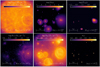 |
Fig. A.1 Morphology of the MC at t ~ 0.5 Myr (cfr. with Fig. 2). |
| In the text | |
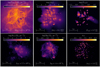 |
Fig. A.2 Morphology of the MC at t ~ 1.4 Myr (cfr. with Fig. 2). |
| In the text | |
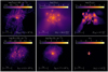 |
Fig. A.3 Morphology of the MC at t ~ 2.0 Myr (cfr. with Fig. 2). |
| In the text | |
|
Fig. B.1 Probability distribution functions (PDFs) for the reference snapshot of the MC simulation. The PDFs are weighted by mass (light blue) and luminosity (blue). Each panel refers to the same snapshot at t ~ 1.1 Myr (the reference snapshot), simulated with 5 × 10⁵ (left panel), 5 × 10⁶ (middle panel), 5 × 10⁷ (right panel) photon packets. Circles indicate the median of each distribution, whereas the dotted lines bracket the 16th and 84th percentiles. |
| In the text | |
|
Fig. C.1 SED statistics for the reference snapshot. The top panel shows the relative error R, the lower panel shows the variance of variance VOV. Blue (red) lines represent the run with 5 × 10⁶ (5 × 10⁷) photon packets, with each line referring to a different observing direction. The dashed lines in both panels indicate the threshold of 0.1 below which the results are reliable. |
| In the text | |
|
Fig. C.2 SED statistics for each snapshot analyzed in this work. The top panel shows the relative error R, and the lower panel the variance of variance VOV. For every snapshot, we show the results relative to the SED of the 6 observing directions, and we color-code the lines relative to each snapshot according to the corresponding time since the beginning of the SF in the MC. The dashed lines in both panels indicate the threshold of 0.1 below which the results are reliable. |
| In the text | |
Current usage metrics show cumulative count of Article Views (full-text article views including HTML views, PDF and ePub downloads, according to the available data) and Abstracts Views on Vision4Press platform.
Data correspond to usage on the plateform after 2015. The current usage metrics is available 48-96 hours after online publication and is updated daily on week days.
Initial download of the metrics may take a while.