| Issue |
A&A
Volume 694, February 2025
|
|
|---|---|---|
| Article Number | A128 | |
| Number of page(s) | 33 | |
| Section | Extragalactic astronomy | |
| DOI | https://doi.org/10.1051/0004-6361/202449593 | |
| Published online | 07 February 2025 | |
The first all-sky survey of star-forming galaxies with eROSITA
Scaling relations and a population of X-ray luminous starbursts
1
Physics Department, & Institute of Theoretical and Computational Physics, University of Crete, GR 71003 Heraklion, Greece
2
Institute of Astrophysics, Foundation for Research and Technology-Hellas, GR 71110 Heraklion, Greece
3
Max-Planck-Institut für extraterrestrische Physik (MPE), Gießenbachstraße 1, 85748 Garching bei München, Germany
4
Remeis Observatory and ECAP, Universität Erlangen-Nürnberg, Sternwartstraße 7, 96049 Bamberg, Germany
5
Eureka Scientific, Inc., 2452 Delmer St., Suite 100, Oakland, CA 94602-3017, USA
6
NASA Goddard Space Flight Center, Code 662 Greenbelt, MD 20771, USA
7
Center for Space Science and Technology, University of Maryland Baltimore County, 1000 Hilltop Circle, Baltimore, MD 21250, USA
8
Center for Research and Exploration in Space Science and Technology, NASA/GSFC, Greenbelt, MD 20771, USA
9
Department of Physics and Astronomy, Johns Hopkins University, 3400 N. Charles Street, Baltimore, MD 21218, USA
⋆ Corresponding author; This email address is being protected from spambots. You need JavaScript enabled to view it.
Received:
13
February
2024
Accepted:
18
November
2024
Abstract
Context. In this work, we present the results from a study of X-ray normal galaxies, that is, galaxies not harbouring active galactic nuclei (AGN), using data from the first complete all-sky scan of the eROSITA X-ray survey (eRASS1) obtained with eROSITA on board the Spectrum-Roentgen-Gamma observatory. eRASS1 provides the first unbiased X-ray census of local normal galaxies, thus allowing us to study the X-ray emission (0.2–8.0 keV) from X-ray binaries (XRBs) and the hot interstellar medium in the full range of stellar population parameters present in the local Universe.
Aims. By combining the updated version of the Heraklion Extragalactic Catalogue (HECATE v2.0) value-added catalogue of nearby galaxies (Distance; D ≲ 200 Mpc) with the X-ray data obtained from eRASS1, we studied the integrated X-ray emission from normal galaxies as a function of their star-formation rate (SFR), stellar mass (M⋆), metallicity, and stellar population age.
Methods. After applying stringent optical and mid-infrared activity classification criteria, we constructed a sample of 18 790 bona fide star-forming galaxies (HEC-eR1 galaxy sample) with measurements of their integrated X-ray luminosity (using each galaxy’s D25) over the full range of stellar population parameters present in the local Universe. By stacking the X-ray data in SFR-M⋆-D bins, we studied the correlation between the average X-ray luminosity and the average stellar population parameters. We also present updated LX-SFR and LX/SFR-metallicity scaling relations based on a completely blind galaxy sample and accounting for the scatter dependence on the SFR.
Results. The average X-ray spectrum of star-forming galaxies is well described by a power law (Γ = 1.75−0.07+0.12) and a thermal plasma component (kT = 0.70−0.07+0.06 keV). We find that the integrated X-ray luminosity of the individual HEC-eR1 star-forming galaxies is significantly elevated (reaching 1042 erg s−1) with respect to what is expected from the current standard scaling relations. The observed scatter is also significantly larger. This excess persists even when we measured the average luminosity of galaxies in SFR–M⋆-D and metallicity bins, and it is stronger (up to ∼2 dex) towards lower SFRs. Our analysis shows that the excess is not the result of the contribution by hot gas, low-mass XRBs, background AGN, low-luminosity AGN (including tidal disruption events), or stochastic sampling of the XRB X-ray luminosity function. We find that while the excess is generally correlated with lower metallicity galaxies, its primary driver is the age of the stellar populations.
Conclusions. Our analysis reveals a sub-population of very X-ray luminous starburst galaxies with higher specific SFRs (sSFRs), lower metallicities, and younger stellar populations. This population drives upwards the X-ray scaling relations for star-forming galaxies and has important implications for understanding the population of XRBs contributing in the most X-ray luminous galaxies in the local and high-redshift Universe. These results demonstrate the power of large blind surveys such eRASS1, which can provide a more complete picture of the X-ray emitting galaxy population and their diversity, revealing rare populations of objects and recovering unbiased underlying correlations.
Key words: galaxies: dwarf / galaxies: starburst / galaxies: star formation / galaxies: statistics / X-rays: binaries / X-rays: galaxies
© The Authors 2025
 Open Access article, published by EDP Sciences, under the terms of the Creative Commons Attribution License (https://creativecommons.org/licenses/by/4.0), which permits unrestricted use, distribution, and reproduction in any medium, provided the original work is properly cited.
This article is published in open access under the Subscribe to Open model. This email address is being protected from spambots. You need JavaScript enabled to view it. to support open access publication.
1. Introduction
The X-ray emission from normal galaxies, that is, those not harbouring active galactic nuclei (AGN), is a prime tool for studying the endpoints of stellar evolution and their effect on their galactic and intergalactic environment. Since this emission is mainly produced by X-ray binaries (XRBs), it is the most efficient way to probe the effectively invisible compact object populations and study their formation and evolutionary paths. As the potential predecessors of gravitational wave sources and short γ-ray bursts (SGRBs; e.g. Marchant et al. 2016), the study of XRB populations and their demographics can provide key insights into the physical processes that drive these phenomena. By constraining the evolutionary channels of XRBs and their formation rates in different galactic environments, we can predict the formation rates of gravitational wave sources and sGRBs over cosmic history and model the high-energy output of galaxies as a function of redshift.
Another notable aspect of XRBs is their effect on their host galaxy and its surrounding intergalactic medium. Given the large mean-free path of high-energy photons, they can affect large volumes around their source. This is of high importance, especially in the high-redshift Universe (z ∼ 30 − 10) where the first XRBs can heat the intergalactic medium and affect the formation of the first galaxies (e.g. Das et al. 2017; HERA Collaboration 2023). XRBs can also energise the interstellar medium of galaxies through photoionisation and the transfer of momentum via jets (e.g. Fender et al. 2005; Schaerer et al. 2019). The formation of XRBs is inextricably connected with the characteristics of the stellar populations in their host galaxies. The study of the association between XRBs and stellar populations of different ages and metallicities is critical for understanding their formation and evolution over cosmic history (e.g. Zezas et al. 2021; Gilfanov et al. 2022).
For these reasons, resolved XRB populations of local galaxy samples have been extensively studied for the characterisation of this correlation. Thanks to the availability of sensitive X-ray observations with the XMM-Newton and Chandra X-ray observatories, it has been shown that the number of XRBs and their total X-ray luminosity can be parametrised in terms of their star-formation rate (SFR), stellar mass (M⋆), and a combination of the two characteristics: the specific SFR (sSFR = SFR/M⋆), which is a proxy to the intensity of star-forming activity (e.g. Mineo et al. 2014; Lehmer et al. 2019; Riccio et al. 2023). Similar scaling relations also hold for the X-ray emitting hot gas in galaxies (Mineo et al. 2012b; Lehmer et al. 2016), which is the result of supernovae (SNe) and massive stars. Recent studies have also shown that metal-poor galaxies tend to host more luminous sources (e.g. Brorby et al. 2016; Fornasini et al. 2020; Kouroumpatzakis et al. 2021), which has important implications for the high-z Universe (Madau & Fragos 2017). In addition, Gilbertson et al. (2022) has shown that the X-ray output of normal galaxies (XRB populations and hot gas emission) can vary as a function of the galaxy’s stellar population age.
A common characteristic of these scaling relations is the increased scatter in the dwarf star-forming galaxies regime (e.g. Gilfanov et al. 2022; Lehmer et al. 2019). This has been attributed to stochastic effects, variations in the stellar population ages and/or metallicity between galaxies, or even variability of individual XRBs (Kouroumpatzakis et al. 2020). Quantifying and addressing the origin of this scatter is very important, particularly for low SFR galaxies (where a few XRBs are expected), both for predicting their X-ray luminosity and for inferring the scaling relations between the X-ray luminosity and the stellar populations of galaxies. Knowledge of these scaling relations provides the formation rate of XRBs (Antoniou et al. 2019), addresses their cosmological evolution (via comparisons with the LX/SFR measured in high-z galaxies, e.g. Lehmer et al. 2016; Aird et al. 2017), and tests their evolution channels via comparisons with XRB population synthesis models (e.g. Fragos et al. 2013).
However, all of these studies so far are based on a small sample (a few hundred galaxies at most) covering only a small fraction of the conditions (SFR, M⋆, metallicity) in the local Universe. This provides only a partial view of the X-ray scaling relations and their scatter (e.g. lacking rare and luminous sources that an all-sky survey can locate).
eROSITA (Predehl et al. 2021), the first 0.2–8 keV all-sky X-ray survey, provides an unbiased census of X-ray galaxies in the local Universe (Basu-Zych et al. 2020). Its results enable the study of these scaling relations by using for the first time a robust and unbiased statistical sample of star-forming galaxies. A first glimpse of its potential has been given by the pilot eFEDS field (140 deg2), which detected 37 spectroscopically confirmed normal galaxies and translated to over 10 000 galaxies in the full eRASS survey (Vulic et al. 2022). These results show that there are galaxies with significant excess with respect to the LX/SFR–sSFR scaling relation for local galaxies (Lehmer et al. 2016). This excess is stronger in lower SFR and lower metallicity galaxies. This indicates that dwarf galaxies with high a sSFR and lower metallicity are more X-ray luminous.
In this work, we use the data from the eRASS1 survey, which allows us to study the LX-SFR-M⋆-metallicity scaling relation for star-forming galaxies using an unprecedented sample of available galaxies (a few thousand). This survey in combination with the Heraklion Extragalactic CATalogue (HECAT; Kovlakas et al. 2021) allows us to define an X-ray unbiased sample by including in our analysis not only X-ray detections but also constraints on the X-ray emission for all galaxies in our parent sample.
This paper is organised as follows. In Sect. 2, we present the X-ray and the galaxy sample used in this work. In Sect. 3, we describe the analysis of the X-ray data, and in Sect. 4, we present the final sample of star-forming galaxies. Section 5 describes the stacking analysis of the X-ray data and the average X-ray template spectrum of the eRASS1 galaxies. In Sect. 6, we present the results of our analysis as well as the results of the fit of the scaling relations. Finally in Sect. 7, we discuss our results and their implications, and in Sect. 8, we present our conclusions.
2. Sample construction
2.1. The eROSITA X-ray survey
eROSITA is an 0.2–8 keV X-ray instrument onboard the Spectrum Roentgen Gamma Observatory (SRG; Sunyaev et al. 2021), which was launched on July 13th, 2019. It consists of seven identical X-ray telescopes each one with a circular field of view (FoV) of ∼1°. The on-axis point spread function (PSF) at 1.5 keV is 15″ (half-energy width, HEW) and it increases with off-axis angle resulting in an average angular resolution of ∼30″ over the FoV (Merloni et al. 2024). The eROSITA All Sky Survey (eRASS) will scan the entire sky 8 times in 6-month intervals providing the deepest view of the X-ray sky to date by the completion of its final scan (eRASS1-8). The eRASS survey provides an unprecedented view of the X-ray sky, free of sample selection biases, which allows studies of source populations and the discovery of rare types of sources.
The X-ray data used in this work are obtained from the first eROSITA all-sky scan (eRASS1) which has been completed in June 2020 reaching a point source average sensitivity of ∼10−14 erg cm−2 s−1 (at the ecliptic equator) in the 0.2–2.3 keV soft X-ray band and ∼2.5 × 10⁻¹³ erg cm−2 s−1 (at the equator) in the 2.3–8 keV hard X-ray band, for a median time exposure (Merloni et al. 2024). In particular, our team has analysed the eRASS1 raw data which belongs to the west hemisphere of the sky covering a region of Galactic longitudes between 180° and 360°.
2.2. Galaxy sample
We use the Heraklion Extragalactic CATalogue, a reference catalogue that contains all known nearby galaxies (204 733 objects) within a distance of D ≲ 200 Mpc (z ≲ 0.048) compiled by Kovlakas et al. (2021). In terms of the B-band luminosity (LB) density, HECATE is almost complete (> 75%) up to distances of 100 Mpc including galaxies with LB down to LB ∼ 1010LB, ⊙, while even farther it reaches a completeness of > 50% up to a distance of 170 Mpc. By incorporating and homogenizing data from the HyperLEDA (Makarov et al. 2014), NED (Helou et al. 1991) databases, and infrared (WISE; 2MASS; IRAS; Wright et al. 2010; Jarrett et al. 2000; Wang et al. 2014) and optical (SDSS; Kauffmann et al. 2003; Brinchmann et al. 2004; Tremonti et al. 2004) surveys, this value-added catalogue provides a broad array of information such as positions, sizes, distances, and stellar population parameters (SFR, M⋆, gas-phase metallicity), and activity classifications. For a detailed description of the catalogue compilation see Kovlakas et al. (2021). Despite the wealth of information included in the first publicly available version of HECATE, the availability of SFR, M⋆, gas-phase metallicity, and activity classification is limited to 46%, 65%, 31%, and 32%, of the full sample respectively. Obtaining a more complete coverage for these parameters is critical for the characterisation of the galaxy sample observed by eRASS1.
For that reason in this work, we use an updated version of the forthcoming catalogue HECATE v2.0. This new version includes the addition of multi-aperture photometric information from mid-infrared (WISE) and optical (SDSS, Pan-STARSS; Flewelling et al. 2020) surveys, as well as spectroscopic data from the SDSS-DR17 spectroscopic database. Furthermore, spectroscopic information from our custom observational campaigns with the Skinakas and TNG telescope is included. In more detail, the HECATE v2.0 Catalogue used in this work provides:
Screening of galaxies with incorrect distances: In the first release of the HECATE catalogue there are a few galaxies (< 0.5%) with wrongly assigned velocities due to misassociatons with foreground stars. In HECATE v2.0 all these cases are flagged allowing the user to exclude these objects from further analysis.
Updated estimations of the SFR and M⋆: The SFR and M⋆ provided by the publicly available version of HECATE are based on the homogenisation of data from different infrared/optical surveys and calibrations. Although this kind of analysis is very useful for large statistical samples, the combination of different calibrations can result to overestimation or underestimation of the SFR and M⋆ of individual galaxies depending on the dust content and the stellar population age of each galaxy. By using the new calibrations of Kouroumpatzakis et al. (2023) HECATE v2.0 provides SFR and M⋆ estimates using a combination of the WISE bands 1 and 3 (W1, W3; 3.4 μm, 12 μm) for the SFR, and WISE band 1, with the optical u-r or g-r SDSS colours for the M⋆, respectively. These new calibrations account for the contribution of old stellar populations in the dust emission for galaxies with low SFR, and for the effect of the extinction providing more reliable estimations for objects over a broad range of star-forming activity. These new calibrations are applied to all HECATE v2.0 galaxies with available and good-quality mid-infrared (WISE) and optical (SDSS) data, while for the rest we used the standard mid-infrared calibration relations from Cluver et al. (2017) and Salim et al. (2014) for the SFR and from Wen et al. (2013) for the M⋆. Special care is taken for the most nearby HECATE galaxies (D ≲ 50 Mpc), where the use of the mid-infrared calibration is not possible because of the low reliability of the catalogue data due to aperture effects. For all these galaxies, the SFR, and M⋆ values from Leroy et al. (2019) catalogue are used. This catalogue provides stellar population parameter estimation for all the nearby galaxies following a more accurate customised analysis for the aperture photometry. Based on this updated analysis in the HECATE v2.0 the availability of SFR, and M⋆ is increased from 46% and 65% to 76% and 90% of the total sample, respectively.
Updated activity classifications. The activity classification of galaxies in the first release of the HECATE is based on spectroscopic information from the MPA-JHU DR8 catalogue (SDSS; Kauffmann et al. 2003; Brinchmann et al. 2004; Tremonti et al. 2004). In particular, using simultaneously four emission-line ratios and an advanced data-driven version of the traditional BPT diagrams, which utilizes a soft clustering scheme, we have available classifications for a large fraction of emission-line galaxies in HECATE (Stampoulis et al. 2019). Although this method is very accurate and robust, since it is based on spectroscopic information, it is limited to the SDSS footprint. To obtain activity classification for a larger fraction of HECATE galaxies, HECATE v2.0 provides updated activity classifications based on the mid-infrared/optical photometric classifier of Daoutis et al. (2023). It is based on the Random Forest (RF) (Louppe 2014) machine learning method, employing the WISE W1-W2 and W2-W3, and SDSS g-r colours. The method is trained on a set of galaxies with high-quality spectra from the MPA–JHU DR8 catalogue characterised using the Stampoulis et al. (2019) diagnostics for the emission line objects and photometric data for the passive galaxies. This new classifier is able to discriminate galaxies in five activity classes: star-forming, AGN, LINER, Composite, and Passive with very high accuracy especially for the star-forming galaxies (> 80%). At the same time, since it is based on photometric data it is applicable to a much larger volume of galaxies for which there are WISE and SDSS (or Pan-STARSS) photometric data. The application of this new method on the HECATE v2.0 galaxies using the additional multi-aperture information from the WISE and Pan-STARSS surveys increased the availability of the activity classification from 30% to 60% of the total sample.
Updated gas-phase metallicities. Gas-phase metallicities in the HECATE v2.0 are based on two methods. For all the galaxies with available emission-line fluxes provided by the MPA–JHU DR8 catalogue, the metallicity is adopted from the available HECATE version (Kovlakas et al. 2021). In particular, following the O3N2 method of Pettini & Pagel (2004, Eq. (3)) (henceforth, PP04 O3N2), Kovlakas et al. (2021) calculated the 12+log(O/H) using the [OIII], [NII], Hα, and Hβ emission line fluxes with S/N > 3 for 62 778 HECATE galaxies within the SDSS footprint. Kewley & Ellison (2008) showed that the PP04 O3N2 method is robust enough, as it is able to trace a wide range of metallicities, with lower scatter, and it is less sensitive to extinction effects. For the galaxies that do not have available spectroscopic metallicities the 12+log(O/H) is calculated based on the mass-metallicity relation using the best-fit results from Kewley & Ellison (2008) for the same spectroscopic calibrator (Table 2). A comparison between the spectroscopically derived metallicity and the one from the mass-metallicity relation shows that within the errors the two methods produce consistent results (Kyritsis et al., in prep.). As a result, given the availability of the updated M⋆ measurements, HECATE v2.0 provides metallicities for a much larger fraction of its galaxies increasing the available values from 30% to 90% of the total sample.
2.3. HECATE-eRASS1 galaxy sample
By combining the HECATE v2.0 value-added information with the eRASS1 data we can study the relation between the X-ray emission of normal galaxies with their stellar population parameters (i.e. SFR, M⋆, metallicity) for the largest galaxy sample so far. To that end, we measured the integrated X-ray flux (see Sect. 3.2) for all the HECATE galaxies within the eRASS1 footprint using the coordinates and the size of each galaxy. The provided galaxy coordinates are very accurate with astrometric precision < 1″ for ∼92% of the galaxies and < 10″ for the remaining objects. The completeness of HECATE in terms of galaxy angular size is 97.6%. For ∼80% of the galaxies, the size information is based on the D25 isophote in the B band, while for the rest this information is obtained mainly from the 2MASS and SDSS, as well as, other catalogues (e.g. 2dFG, WINGS etc.). All the supplementary sizes have been rescaled based on the reference semi-major axis provided by HyperLEDA. For a detailed description of the galaxy position and size information see Kovlakas et al. (2021). To avoid galaxies with problematic distances, due to misassociations with foreground stars, we removed 956 cases flagged as ‘Star_contamination = Y’ (see Sect. 2.2). This results in an initial sample of 93 806 HECATE galaxies that have been observed by eRASS1 (hereafter HEC-eR1) in the west hemisphere of the sky.
2.4. Selection of bona fide star-forming galaxies
To select all the normal galaxies within the HEC-eR1 sample we utilised the activity classifications provided by HECATE v2.0 (see Sect. 2.2).
First, we selected all galaxies within the HEC-eR1 sample classified as star forming based on both the spectroscopic (SP) and the photometric (RF) classification (SP = 0 & RF = 0). Afterwards, we included in our sample also star-forming galaxies with available spectroscopic classification, but without available photometric classification (SP = 0 & RF not available). Since we consider the spectroscopic classification as the ground truth, we also included star-forming galaxies with available spectroscopic classification and a contradicting photometric classification (SP = 0 & RF ≠ 0). Finally in order to increase the completeness of our final sample we considered also galaxies for which there is no available spectroscopic classification but the photometric activity diagnostic tool classifies them as star forming (SP not available & RF = 0). Given that the two methods predict the probability of a galaxy to belong in each activity class (see Stampoulis et al. 2019; Daoutis et al. 2023), we included in our final sample only the star-forming galaxies with a probability PSFG > 75%. This probability threshold is well-calibrated for both methods ensuring the star-forming nature of these galaxies. This resulted in a final sample of 20 392 star-forming galaxies within HEC-eR1 sample. Table 1 summarizes the construction of the star-forming galaxies HEC-eR1 sample based on the different criteria described above. The majority of the star-forming galaxies in our sample (14 739/20 392) have spectroscopic confirmation (PSFG > 75%) while for the remaining 5653 outside the SDSS footprint, the star-forming classification is robust given the very high performance of the photometric classifier (RF) on predicting star-forming galaxies based on their mid-IR and optical colours (Daoutis et al. 2023).
Sample selection criteria for the star-forming galaxies within the HEC-eR1 sample.
To estimate the contamination in the HEC-eR1 galaxy sample, for which we do not have any spectroscopic information, by other galaxy types we performed the following analysis. First, we defined an initial sample for which we have photometric (RF) activity classifications and for comparison we also have spectroscopic (SP) activity classifications, without setting a probability threshold. This results in 16 564 galaxies of all activity types. Afterward, by considering the spectroscopic classification as the ground truth, we calculated how many spectroscopically confirmed non-star-forming galaxies were classified as star forming with PSFG > 75% by the photometric diagnostic. We found that only 212/16 564 galaxies have been misclassified as star forming by the photometric diagnostic. Based on this we consider that the photometric only classification of the star-forming galaxies in our final HEC-eR1 sample is robust with a false positive rate of ∼1%.
3. X-ray data analysis
3.1. eRASS1 data reduction
Since we are interested in the integrated X-ray emission of the galaxies, we extracted the eRASS1 spectra and auxiliary files using version 1.72 of the srctool task contained in version eSASSuser211214 of the eROSITA Science Analysis Software System (eSASS, Brunner et al. 2022) from event data of processing version 010. The source regions were defined using the D25B-band isophote size of the galaxies, which is defined as an ellipse with the semi-major axis (R1), the semi-minor axis (R2), and the position angle (PA) provided by the HECATE catalogue. For less than 10% of the galaxies the extraction radius was smaller than the FoV average HEW of the eROSITA PSF. We did not attempt to perform extractions for a larger aperture in order to avoid excess contamination by background emission that might be present in the larger aperture. In any case, the aperture corrections for this small extraction region are included when we calculate the source flux through the ARF. For the HEC-eR1 galaxies without size information (PGC2807061, PGC24634), we considered a circular aperture with a radius of 1′. The first galaxy is a low-mass dwarf irregular galaxy that contains a modest H II region (Silva et al. 2005) at a distance of 3.36 Mpc. The second galaxy is a typical SB galaxy at a distance of 22.65 Mpc. Visual inspection of their optical DSS images guarantees that we do not omit flux from the galaxy’s main body by selecting this circular aperture. Background X-ray spectra were extracted from a circular annulus around the central position of each galaxy. We set the inner radius of this annulus to 60″ if the semi-major axis of the respective galaxy is smaller, and 10″ larger than the semi-major axis otherwise. For the outer radius we adopted values 150″ larger than the inner radius. All detections listed in the main source catalogue of eRASS1 were excluded from the background regions. In order to avoid the removal of any potential X-ray emitters that belong to the galaxy (i.e. Ultra Luminous X-ray sources; ULXs) we did not mask any detected source into the source aperture. However, in Sect. 5.4 we estimate the contamination from background AGN in HEC-eR1 sample based on a statistical approach.
3.2. X-ray source photometry
In order to measure the observed counts we summed up the measured counts in the source and the background spectrum of each galaxy in the soft (S) 0.6–2.3 keV and hard (H) 2.3–5.0 keV eROSITA bands. We used the Sherpa v.4.15.1 package (Freeman et al. 2001; Doe et al. 2007; Burke et al. 2023). Because more than 95% of our sources have ≤5 counts above the background the source net counts could not be simply calculated by subtracting the estimated background counts from the source counts. Instead, we calculated the posterior distribution of the source counts given the observed counts in the source and background apertures, and the Bayesian formalism of van Dyk et al. (2001) as implemented in the BEHR1 code (Park et al. 2006). BEHR accounts also for differences between the source and background effective areas, and exposure times. The selection of the prior distribution is important since it may drive the shape of the posterior distribution in this low-count regime. After a sensitivity analysis for different assumptions for source and background counts and priors, we found that a non-informative prior in the log scale has the least effect on the posterior distribution for sources with a few observed counts. The posterior distribution was calculated by using the Gibbs sampler drawing 20 000 draws (burn-in: 4000). In the subsequent analysis we use the full set of draws from the posterior count distribution.
3.3. X-ray fluxes, luminosities, and X-ray colour
To calculate the X-ray fluxes in the 0.6–2.3 keV eROSITA’s most sensitive (Predehl et al. 2021) band, the posterior count distribution (calculated as described in Sect. 3.2) was multiplied by the count-rate to flux conversion factor of each galaxy in our sample. Although this conversion depends on the spectral model that better describes the X-ray spectrum (e.g. Zezas et al. 2006), the low number of counts of our sources does not allow us to fit each of them separately. Since the Ancillary Response File (ARF) and the Redistribution Matrix Function (RMF) are different for each sky location we calculated the count-rate-to-flux conversion factor for each galaxy by convolving the average spectrum of the HEC-eR1 galaxies (see Sect. 5.1) with the ARF and RMF file for each galaxy. As we discuss in Sect. 5.1 and in the Appendix A, this choice is justified by the fact that there is no indication for spectral evolution as a function of the SFR and M⋆ of the galaxies in our sample. The spectral model consists of a power-law component (Γ = 1.75), a thermal component (APEC; kT = 0.70 keV, Z = Z⊙) that contributes ∼13% of the total flux (see Sect. 6.2). Both are absorbed by cold gas modelled with the Tuebingen-Boulder (tbabs) ISM absorption model (Wilms et al. 2000). The neutral hydrogen column density, NH, is calculated independently for each galaxy using the survey of Dickey & Lockman (1990) and the colden tool, which is part of proposaltools provided by CIAO (Fruscione et al. 2006).
Throughout this paper, we use the soft 0.5–2.0 keV X-ray bands for comparison with other works. The flux and the corresponding luminosity in this band were calculated by converting the measured flux in the 0.6–2.3 keV eROSITA band assuming the above-mentioned absorbed power-law + APEC model. For simplicity, and to facilitate future comparisons with other works we adopted the same absorbing NH for all galaxies, which is the median NH = 3.06 × 1020 cm−2 of the star-forming galaxies in the HER-eR1 sample, given that the dispersion of the conversion factors (using the individual NH) is less than 2%. The conversion factor from our analysis band (0.6–2.3 keV) to the adopted soft (0.5–2 keV) is,  . For comparison with other works the conversion factor from the 0.6–2.3 keV to the full 0.5–8 keV band, assuming the same model is
  , respectively. When needed, we convert luminosities from other works to our adopted band based on the spectral models used in each corresponding study. All the conversion factors used throughout this work are presented in Table 2.
The conversion factors used throughout this work.
In addition, we also calculated the X-ray colour of the galaxies in our sample, which is defined as  , where S and H are the source counts in the two bands. Given that our galaxies have only a few counts we calculated the posterior distribution of the X-ray colour using again the BEHR code (Park et al. 2006). In addition, during the calculation we took into account the variations in the ancillary response files of each galaxy due to their different position on the detector.
3.4. Reliability of the X-ray flux measurements
Although our approach of calculating the full posterior distribution of the source flux can deal with very faint sources, there are cases of extremely low-count sources where their posterior count distribution is very wide and positively skewed with a mode very close to zero. That means that the posterior intensity of such sources is almost zero not allowing us to handle them as point measurements given their very large uncertainties. In order to estimate which galaxies in our sample have reliable flux measurements we utilised the posterior distribution of the source counts in the 0.6–2.3 keV eROSITA band and we calculated its mode value Smode and its lower Slow, 68%, and upper bound Sup, 68% at the 68% confidence interval (C.I.). Based on the shape of the posterior, we considered as reliable measurements all the galaxies for which
 (1)
(1)
Flux measurements for which this criterion is not satisfied are considered as uncertain. In Fig. 1 we present two examples of sources in our sample with reliable flux measurement and with an uncertain flux measurement. The red and green error bars indicate the upper and lower bounds of the distribution at the 68% and the 90% C.I., respectively. The vertical black solid line indicates the mode value of the distribution. The posterior distribution of the reliable source (top panel) is more symmetric and its mode value is ≳30 counts. On the other hand, the posterior distribution of the source with uncertain flux measurement is strongly positively skewed with a mode of almost zero. This example demonstrates that our criterion of assessing the reliability of the flux measurement for a source (Eq. (1)) is robust and can characterize well the galaxies in our sample. In this way, we found 93 secure star-forming galaxies with reliable flux point estimates while the remaining 20 299 have uncertain flux point estimates. For visualisation purposes, throughout this paper, we use as a point estimate the mode of the flux distribution for the reliable galaxies and the error bars correspond to the 68% C.I. On the other hand, we adopt the upper 90% C.I. of the flux distribution for the galaxies with uncertain flux measurements. However, when performing the maximum-likelihood fit for the scaling relations (see Sect. 6.5), we consider the complete posterior flux distribution for each galaxy (reliable and uncertain) rather than relying on a single value measurement. In Fig. 2 we show the distribution of our reliably measured fluxes (black stars) and the galaxies with uncertain fluxes (grey down arrows) in the 0.6–2.3 keV band as a function of the exposure time. The reliable flux measurements are spanning a range from 10−11 erg cm−2 s−1 to ∼10−14 erg cm−2 s−1, while the exposure time for all the galaxies in our sample is in the order of a few hundred seconds. We do not see a trend for longer exposures to be associated with more reliable flux measurements. This is because the posterior distribution depends on the local background and the size of the extraction aperture.
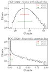 |
Fig. 1. Example of the posterior count distribution of two sources in our sample for which we have reliable and unreliable flux measurement as defined based on the Eq. (1). The red and green error bars indicate the upper and lower bounds of the distribution at the 68% and the 90% C.I., respectively. The vertical black solid line indicates the mode value. |
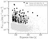 |
Fig. 2. Flux distribution in the 0.6–2.3 keV band of the star-forming galaxies in the HEC-eR1 sample as a function of the exposure time. Black stars show the mode value of the source’s intensity for the galaxies with reliable fluxes and their 68% C.I. uncertainties. Grey down arrows show the upper 90% C.I. for the galaxies with uncertain flux measurements. |
In order to assess the robustness of these flux measurements, we cross matched the entire sample of HEC-eR1 galaxies (including the eR1 objects with uncertain flux measurements) with the catalogue of all available Chandra observations, and the 4XMM-DR13s catalogue of sources detected in stacked XMM-Newton observations (Webb et al. 2020). In both cases we used a search radius of 15″. This resulted in 86 and 95 HEC-eR1 galaxies with available Chandra observations or XMM-Newton detections. In order to simplify the analysis of these data, for the Chandra observations we only kept sources that fitted within one chip of the ACIS detector, and for the XMM-Newton observations we only kept galaxies with angular extent smaller than ∼15″ and good quality detections (summary flag < 3). We analysed the Chandra data with the CIAO v4.15 software package. After the application of standard screening criteria, we measured the count rate in the 0.6–2.3 keV band within the galaxy aperture using the same apertures as in the eRASS1 analysis. The background regions were adjusted to fit within the limited field of the same detector chip as the galaxy. The net source counts were calculated using the BEHR code with the same parameters as for the eRASS analysis (Sect. 3.2). We also calculated the count-rate to flux conversion factors based on ARFs derived for each Chandra OBSID individually and the average spectrum described in Sect. 5.1. In the case of the XMM-Newton data we used the spectra and ARFs available from the pipeline products for each source. In Fig. 3 we plot the logarithm of the ratio of the eR1 fluxes over the fluxes derived from the Chandra or XMM-Newton data, as a function of the Chandra/XMM-Newton fluxes in the 0.5–2 keV band. The galaxies with uncertain eR1 flux measurements with available reliable X-ray flux measurements with these other instruments are shown with black down-arrows. This comparison indicates that within the uncertainties the fluxes are reasonably consistent with a scatter ∼0.5 dex which may be the result of variability (e.g. due to ULXs, which in some cases were the targets of these observations) and/or aperture effects.
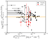 |
Fig. 3. Comparison between the X-ray fluxes measured from the eRASS1 extractions (Sect. 3.3) and those derived from archival Chandra and XMM-Newton observations. The orange line corresponds to the line of equality. We find good agreement with a scatter of ∼0.5 dex, supporting the robustness of the eRASS1 extractions. |
4. Final sample of star-forming galaxies
4.1. Stellar population properties for the HEC-eR1 secure star-forming galaxies
In order to study the correlation between the integrated X-ray emission and the stellar population parameters of the host galaxy, we need accurate and realistic estimations of the SFR, M⋆, and metallicity of the galaxies in our sample. For that reason, we utilised the values provided by the HECATE v2.0 catalogue (see Sect. 2.2). In particular, we selected only the star-forming galaxies within the HEC-eR1 sample with SFR > 10−3 M⊙ yr−1 because for lower values the incomplete sampling of the stellar initial mass function (IMF) will lead to large fluctuations (e.g. Kennicutt & Evans 2012). We also opted to use only galaxies with M⋆ > 107 M⊙ because lower estimations can be unrealistic indicating that they most likely were derived from unreliable photometry, and suffer from aperture effects. These cuts result in 18 894 secure star-forming galaxies (91 with reliable X-ray flux measurements, and 18 803 with uncertain X-ray flux measurements).
For the majority of the star-forming HEC-eR1 galaxies the SFRs and M⋆s were based on the calibrations of Kouroumpatzakis et al. (2023) (58% or 10 960/18 994, and 62.8% or 11 859/18 894, respectively). For 27% of the galaxies, the SFRs are based on the calibrations of Cluver et al. (2017) and for the remaining 15% the SFR values from Salim et al. (2014) and Leroy et al. (2019) were adopted (14.8% and 0.2%, respectively). On the other hand, the M⋆s for the rest 37.1% (7019/18 894) are based on the calibrations of Wen et al. (2013) and only for a 0.1% (16/18 894) the M⋆s proposed by Leroy et al. (2019) were adopted. The use of these different calibrators is dictated by the available photometric data for each galaxy. As discussed in Kouroumpatzakis et al. (2023) and Kyritsis et al. (in prep.) there is a systematic offset of about 0.2 dex between the two main calibrations we use for the SFR and M⋆ calculations, which is consistent with the scatter of these calibrators. Finally, the vast majority of the gas-phase metallicities in our sample (70% or 13 206/18 894) were derived using the PPO3N4 spectroscopic method (Kewley & Ellison 2008) while for the rest of the galaxies (30% or 5688/18 894) are based on the mass-metallicity relation for the same metallicity calibration (see Sect. 2.2). The systematic offset between the two metallicity calibrations for the spectroscopically confirmed star-forming galaxies in our sample is less than ∼0.1 dex which does not introduce additional scatter on the metallicity estimations due to different calibrations.
4.2. AGN screening
In Sect. 2.4 we selected all the star-forming galaxies in the HEC-eR1 sample based on stringent activity classification criteria. Nevertheless, the measured X-ray flux can be still contaminated by photons originating from a background AGN that is in projection with the galaxy. To exclude such cases from our final sample of secure star-forming galaxies, we cross-matched them with the all-sky AGN catalogue from Zaw et al. (2019). This catalogue includes spectra from the SDSS and 6dF Galaxy surveys (6dF; Jones et al. 2004, 2009), supplemented by private spectra obtained with the long-slit FAst Spectrograph for the Tillinghast telescope (Fabricant et al. 1998, FAST) and the R-C grating spectrograph on the V.M. Blanco 4.0 m telescope at the Cerro Tololo Inter-American Observatory (CTIO). This makes it one of the largest, all-sky spectroscopic AGN catalogue in the nearby Universe (z < 0.09). The sample consists of 1929 broad-line AGNs and 6562 narrow-line AGNs. However, we notice here that this catalogue is based on lower resolution spectra than the SDSS spectra used in the HECATE catalogue. For that reason, we did not crossmatch the entire HECATE with this AGN catalogue. Instead, we handled it carefully after a detailed inspection of its provided classifications. The classification of the AGNs is based on emission line ratio measurements using the standard two-dimensional diagnostics from Kewley et al. (2001) and Kauffmann et al. (2003). The crossmatch returned 248 matches. For consistency with the spectroscopic classifications in HECATE, and given that the 4-D diagnostics of Stampoulis et al. (2019) are more robust than the 2-D projections used in Zaw et al. (2019), we removed only galaxies for which the two activity classifications agreed. For the classification, we used the same emission line quality cuts as the ones applied in the HECATE catalogue. We found that 41 out of 248 galaxies were also classified as AGNs from our diagnostic and we removed them from our final sample. More than 90% of the remaining galaxies were classified either as star forming or composites, which are closer to the star-forming locus of the emission-line diagnostic diagram.
To further ensure the star-forming nature of our galaxies, we visually inspected the X-ray/optical images and optical spectra (where available) of all the 91 star-forming HEC-eR1 galaxies with reliable flux measurements. We removed the galaxies PGC4125797 and PGC78895, since their X-ray and optical images showed that their X-ray emission is coincident with a spectroscopically confirmed background AGN. In addition, we excluded two galaxies (PGC28415, PGC36648) for which the inspection of their optical spectra indicates a clearly broad-line AGN. We also cross-matched all the 91 star-forming HEC-eR1 galaxies with reliable flux measurements with the NED database to investigate for additional evidence for AGN activity. We removed two galaxies (PGC36126, PGC1809432) which belong to the work of Liu et al. (2019) who presented a comprehensive and uniform sample of broad-line AGN using spectra from the SDSS DR7. Furthermore, we discarded the galaxy PGC38964 which is characterised as a Compton-thick AGN in the work of Tanimoto et al. (2022) who performed a systematic broadband X-ray spectral analysis of 52 Compton-thick AGN (CTAGN) candidates selected by the Swift/Burst Alert Telescope all-sky hard X-ray survey (Ricci et al. 2015).
Given the very large number of star-forming galaxies with uncertain flux measurements (20 299) it was not possible to inspect the images/spectra and bibliography for all of them. Instead, we randomly selected a subsample of 50 galaxies and we repeated the visual inspection and the literature search only for them. We removed the galaxy PGC2082767, since it is classified as a Seyfert galaxy based on its emission line measurements from Hopp et al. (2000). In addition, although its optical spectrum indicates a star-forming galaxy, we did not include PGC1139676, a spectroscopically confirmed background AGN, which could potentially contaminate the measured X-ray emission projected on the body of the galaxy. This analysis suggests that the AGN contamination of the overall population of the star-forming galaxies with uncertain flux measurements (20 299) is ∼4%. This is of the same order as the false positive rate estimated in the Sect. 2.4.
In addition, another source of potential contamination of the measured X-ray flux could be a time-variable (or transient) nuclear accretion episode not accounted for in the spectroscopic or photometric classification. This possibility is discussed in Sect. 7.5.
So far, we screened our sample for all the galaxies associated with an AGN based on the visual inspection of their X-ray/optical images, and an extensive literature search. However, heavily obscured AGNs or unobscured low-luminosity AGN (LLAGN) (Merloni et al. 2014) can still contaminate the measured X-ray emission. To find such cases, we compared the calculated X-ray colour C (see Sect. 3.3) of our secure star-forming galaxy sample with the expected X-ray colour from a heavily obscured AGN, assuming an absorbed power-law model with photon index values Γ = 0, or 1 and a typical NH = 1020 cm−2. This analysis resulted in the removal of 2 galaxies (PGC55410, PGC52042) with colours consistent with a very hard spectrum similar to those of an obscured AGN. In the end, based on our screening process we rejected 52 potentially AGN-contaminated galaxies.
X-ray variability is a tell-tale signature of AGN activity. The recent study of Arcodia et al. (2024) identified a sample of AGN based on X-ray variability detected in the eRASS data. A cross-correlation of our sample of star-forming galaxies with the variable sources in this analysis did not yield any matches, indicating that there are no strongly variable known AGN within our sample.
4.3. Screening for star-forming galaxies with galaxy cluster associations
Another known contaminant that could affect the measured X-ray fluxes of normal galaxies is the association of our star-forming galaxies with foreground or background galaxy clusters. For that reason, we cross-matched the HEC-eR1 sample with the eRASS1 galaxy cluster catalogue (Bulbul et al. 2024). For the crossmatch we used the Sky with Errors matching algorithm provided by TOPCAT (Taylor 2005). Given the positions of the HEC-eR1 galaxies and the positions of the detected X-ray clusters we searched for matches using as positional errors the galaxy’s semi-major axis (R1) and two times the radius of the detected cluster, respectively. In this way, we ensured that each galaxy is within the extent of the cluster. This resulted in 415 matches 12 of which are star-forming HEC-eR1 galaxies, and for that reason we removed them from our final sample. Given that the eRASS1 is a flux-limited survey, it is possible to not detect the soft X-ray emission of extended nearby clusters (e.g. Virgo, Fornax, Coma etc.). Since this may contaminate the signal in the stacked data (Sect. 5.2) and the average X-ray spectrum of the star-forming galaxies (Sect. 5.1) we also cross-matched the HEC-eR1 galaxy sample with the Abell and Zwicky Clusters of Galaxies catalogue (Abell 1995). By using again the same matching algorithm (Sky with Errors) and as positional errors the R1 and the radius of the cluster, we removed 30 secure star-forming galaxies positionally coincident with clusters. X-ray emission from compact galaxy groups may also contaminate the X-ray emission we measured if the galaxy coincides with the extended X-ray emission from a galaxy group. For this reason we cross-matched the HEC-eR1 galaxies with the compact group catalogue of Hickson (1982). Using Sky with Errors and as positional errors the galaxy’s R1 and the radius of the group, we removed 10 secure star-forming galaxies associated with compact groups of galaxies. Following the screening process described above, we removed 52 star-forming galaxies from our sample which were associated either with galaxy clusters or with compact groups of galaxies. In Table 3 we summarize all the steps we followed for the construction of the final HEC-eR1 sample of star-forming galaxies.
Sample size in each step of the screening process for the construction of the final HEC-eR1 sample of star-forming galaxies.
4.4. HECATE - eRASS1 final sample of star-forming galaxies
Our final clean sample of secure star-forming HEC-eR1 galaxies is comprised of 18 790 galaxies out of which 77 have reliable X-ray flux measurements and the remaining 18 713 have uncertain fluxes. Despite that the majority of the galaxies that we removed during the AGN and galaxy cluster screening were characterised as uncertain X-ray flux measurements, we followed this approach in order to avoid any contamination during the stacking of the X-ray spectra (see Sect. 5.2). In addition, although the number of galaxies with uncertain X-ray fluxes dominates our final sample, we include them in our analysis in order to avoid biasing our results. In fact, our methodology for the fitting of the scaling relations utilizes the posterior distribution of the X-ray luminosity of each galaxy (as it was derived from the flux posterior distribution and the corresponding distance; see Sect. 3.3) instead of the point estimation of the luminosity (see Sect. 6.5). In Fig. 4 we present the distribution of the final HEC-eR1 sample of secure star-forming galaxies in the SFR-M⋆-D-metallicity parameter space. In both panels, stars indicate the galaxies with reliable X-ray flux measurements, and the dots the galaxies with uncertain fluxes. The colour-code in the top panel depicts the logarithm of the distance of each galaxy while in the bottom panel the gas-phase metallicity, 12+log(O/H). The diagonal dashed lines indicate three different sSFR values (i.e. sSFR: 10−9, 10−10, and 10−11 M⊙ yr−1/M⊙). The orange solid line shows the main sequence of the star-forming galaxies from Renzini & Peng (2015). Our sample is well distributed in the SFR-M⋆ plane (i.e. main sequence plane) spanning a range of SFR = 10−3 − 25 M⊙ yr−1 and a range of M⋆ = 107 − 5 × 10¹¹ M⊙ from dwarf star-forming galaxies to large starburst galaxies. All the galaxies are symmetrically distributed around a sSFR of 10−10 M⊙ yr−1/M⊙ while the reason that we find slightly more nearby galaxies in lower sSFRs is because the quality of our photometric data do not allow us to accurately calculate the SFR and the M⋆ of very distant galaxies. In addition, our sample covers a relatively wide range of metallicities from 12+log(O/H) = 8.0 sub-solar to 12+log(O/H) = 9.0 super-solar. The distribution of our final sample in the SFR-M⋆-D-metallicity parameter space allows us to study the correlation between the widest range of host galaxy properties and the integrated LX for the first unbiased X-ray sample of star-forming galaxies in the local Universe. In Table B.1 we present the properties of the HEC-eR1 sample of star-forming galaxies with reliable flux measurements.
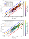 |
Fig. 4. Distribution of the final clean sample of the secure star-forming HEC-eR1 galaxies in the main sequence plane. In both panels, stars indicate the galaxies with reliable X-ray flux measurements, and the dots the galaxies with uncertain fluxes. The colour-code in the top panel corresponds to the log(D), while in the bottom panel corresponds to the gas-phase metallicity, 12+log(O/H). The diagonal dashed lines indicate three different sSFR values (i.e. sSFR: 10−9, 10−10, and 10−11 M⊙ yr−1/M⊙). The orange solid line shows the main sequence of the star-forming galaxies from Renzini & Peng (2015). Our final sample is well distributed along the SFR-M⋆ plane covering a wide range of distances and gas-phase metallicities. |
5. X-ray stacking analysis
5.1. Average X-ray spectrum of the galaxy sample
As it is seen in Fig. 2, eRASS1 is a relatively shallow survey with an average exposure time of the order of a few hundred seconds. This means that for the vast majority of the galaxies in our sample, the low number of observed counts does not allow us to calculate a count-rate to flux conversion factor based on the X-ray spectrum of each galaxy. Instead, we stacked the X-ray spectra of all the 18 790 star-forming galaxies within our final HEC-eR1 sample. In this way, we can study the average X-ray properties of the galaxy population by using their combined X-ray spectrum (which is representative of all the galaxies in our sample and it has a much higher S/N). Using the combine_spectra command provided by the Sherpa v.4.15.1 package and by setting the parameter method=‘sum’ we summed all the source spectra, the associated response files (ARF and RMF), and the background spectra. The output combined spectrum contains the sum of all source counts. To combine the background counts and to compute the background to source area scaling (backscal) values, we set the parameter bscale_method=‘time’. This method computes the total unweighted counts for the source and background spectra and provides the exposure time-weighted background scaling value which corresponds to the fraction of the background counts included in the source spectrum. In addition, the combined response files and the combined background are also provided. In Fig. 5 we present the final average X-ray spectrum of the secure star-forming galaxies in our sample.
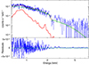 |
Fig. 5. Stacked X-ray spectrum of all the secure star-forming galaxies within the HEC-eR1 sample. The green and red lines show the power-law and hot plasma model components, respectively. The orange line corresponds to the best-fit model. |
By using again the Sherpa v.4.15.1 package we fitted the X-ray spectrum with a spectral model which includes an absorbed power-law and a thermal plasma (APEC; Smith et al. 2001) component. The former describes the X-ray emission produced by typical XRBs populations, and the latter accounts for the diffuse emission due to hot gas in the galaxy. Foreground absorption was modelled through the tbabs ISM absorption model (Wilms et al. 2000). The average spectral model was tbabs×(power-law + APEC). The fit was performed within the eROSITA’s most sensitive band (i.e. 0.6–2.3 keV) since above ∼2.5 keV the spectrum is background dominated. However, for plotting purposes we also show the extrapolation of the best-fit model up to 8.0 keV. In order to subtract the background and to use the χ2 statistics the spectrum was binned to have at least 10 counts per bin. The best-fit model parameters for the integrated average spectrum are presented in Table 4. In order to estimate the uncertainties in the spectral parameters, we used the confidence Sherpa task. This task computes confidence interval bounds by varying a given parameter’s value over a grid of values while all the other thawed parameters are allowed to float to new best-fit values. We adopted as an error in the best-fit parameters the 1σ (68%) confidence interval. The best-fit model is overplotted with an orange line, while the red and green lines indicate the absorbed power-law and the thermal plasma components, respectively.
Best-fitting model spectral parameters for the average X-ray spectrum of all the HEC-eR1 star-forming galaxies.
We see that the average X-ray spectrum of all the galaxies in our sample is dominated by a power-law component with a photon index  , and a hot plasma temperature,
  keV which is typical for the sub-keV temperatures of hot gas in the star-forming galaxies (Owen & Warwick 2009). In addition, the fact that we did not detect a flat, hard X-ray tail in the spectrum or the presence of the Fe-Kα 6.4 keV line strongly indicates that our sample is fairly clean of obscured AGNs (cf. Ballo et al. 2004).
As we see in Table 4 this two-component model gives a very good fit (reduced – χ2 = 0.65) without showing any systematic residuals. Nevertheless, we tried to fit our stacked spectrum with more complex models. In particular, we added a second APEC component to account for a multi-temperature thermal plasma, or we explicitly accounted for absorption in the dusty star-forming regions by including an additional absorber to the power-law component (e.g. Mineo et al. 2012b; Garofali et al. 2020; Lehmer et al. 2022). The resulting fits were completely unconstrained, and the fit statistic was not significantly improved. For that reason, we did not consider any more complex models.
In Sect. 3.3 we used these results, in order to calculate the count-rate-to-flux conversion for each galaxy. However, before we adopt a common spectral model for the entire sample of galaxies, we examined for spectral variations between the average spectra of different SFR-M⋆ bins. This analysis showed that there is no clear indication of evolution in the spectral parameters per SFR-M⋆ bin (Appendix A). In addition, to test if our stacking procedure is driven by the brightest sources in each bin, we examined the distribution of our galaxies with reliable flux measurements (i.e. the brightest sources in the sample) on the SFR-M⋆ plane, as a function of their net number of counts in the 0.6–2.3 keV band. Our analysis showed that there is no trend for the brightest galaxies to be in a specific region of the SFR-M⋆ parameter space. In fact, 90% of the net counts of the sources with reliable flux measurements, comes from galaxies with SFR < 2 M⊙ yr−1. Therefore, although the brightest galaxies may have a stronger contribution in the stacked spectrum they should not bias the spectral parameters in any particular direction or any particular stacks.
5.2. X-ray stacking analysis per SFR–M⋆–D bins
In order to compute the mean X-ray luminosity of our population of star-forming galaxies we stacked our sample in SFR-M⋆-D bins. Given that the population of the 18 790 individual galaxies is not uniformly distributed along the main sequence plane (Fig. 4), we followed an adaptive binning approach in order to ensure an adequate number of galaxies in each bin. The binning scheme is presented in Table 5 and it is shown on the SFR-M⋆ plane in Fig. 6. This resulted in 239 occupied SFR-M⋆-D bins and 107 of them include more than ten galaxies. By following the same stacking procedure as in Sect. 5.1, we stacked the source spectra of all the individual galaxies in each one of these 239 SFR-M⋆-D bins, and we obtained one combined spectrum per bin. In this way, we increased the X-ray signal even for the bins which were dominated by galaxies with uncertain flux measurements. Afterward, by performing the same analysis as described in Sect. 3.2 we derived the posterior X-ray count distribution of each stacked spectrum and based on this we calculated the X-ray fluxes and luminosities as in Sect. 3.3. These are the average X-ray flux and X-ray luminosity of the galaxies in each SFR-M⋆-D in the 0.6–2.3 keV energy band. For the calculation of the luminosities in the 0.5–2 keV and the 0.5–8 keV energy bands, we used the median distance of the galaxies in each SFR-M⋆-D bin and the conversion factors c1 and c2 (see Table 2). In addition, we used the count-rate to flux conversion factors based on the average galaxy spectrum (Table 4) and the response files calculated from the stacking analysis for each bin (see Sect. 3.3). Although the stacking of a large number of individual galaxies per bin with uncertain flux measurements will lead to a combined posterior distribution with a larger number of counts, for a number of bins this does not necessarily lead to a reliable flux measurement. This is the case in the low or the high end of the SFR and M⋆ parameter range where the number of individual galaxies in each bin is very small resulting in a small increase of the total number of counts in comparison to the individual galaxies. To characterize the flux measurements of the stacked data we used the shape of the final posterior count distribution as it was described in Sect. 3.4. We found 58 stacks with reliable flux measurements and 181 with uncertain flux measurements. In Fig. 6 we present the final distribution of the stacks per SFR-M⋆-D bin. Blue squares correspond to the stacks with reliable flux measurements and the circles of the same colour to those with uncertain flux measurements. We note here that for visualisation purposes we show the bin scheme only in the SFR-M⋆ plane. As a result, each region defined by the dashed lines is not a single bin but further split into nine D bins. Therefore within each SFR-M⋆ bin (regions defined by the dashed black lines) there are more than one stacks. For comparison, we overplot the individual galaxies with reliable flux measurements (black stars) and the galaxies with uncertain fluxes (grey circles). The black dashed lines indicate the SFR-M⋆ bins. To study the correlation of the mean X-ray luminosity with the average stellar population parameters of the galaxies, we calculated the mean SFR and the mean M⋆, as well as the median metallicity of the galaxies in each SFR-M⋆-D bin.
Adopted bins in the SFR, M⋆, D dimensions.
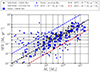 |
Fig. 6. Distribution of SFR-M⋆-D bins on the main sequence plane. Each bin is characterised by the mean SFR and M⋆ of the galaxies contained in each bin. Blue squares correspond to the stacks with reliable X-ray flux measurements based on the X-ray stacking analysis and the blue circles to those with uncertain flux measurements. Black stars show the individual galaxies with reliable X-ray flux measurements and the grey circles the galaxies with uncertain fluxes. The black dashed lines indicate the SFR and M⋆ range of the bins. The diagonal dashed lines indicate three different sSFR values (i.e. sSFR: 10−9, 10−10, and 10−11 M⊙ yr−1/M⊙). |
5.3. X-ray stacking analysis with bootstrap sampling
In Sect. 5.2 we discussed how we calculated the average X-ray luminosity of the galaxies in our sample as a function of their SFR and M⋆ properties by stacking the X-ray spectra of the individual galaxies in SFR-M⋆-D bins. However, in order to assess the variance of the calculated average X-ray luminosity we utilised the bootstrap sampling technique which is widely used in similar works (e.g. Lehmer et al. 2016; Fornasini et al. 2019). Bootstrap sampling allows us to quantify the uncertainty of the mean X-ray luminosity, and assess how the individual galaxies affect the average stacked signal in each SFR-M⋆-D bin. To do that, we started from the initial list of galaxies in each bin, and we created 100 “similar” galaxy lists by resampling the initial list. More specifically, each of the new lists was constructed by randomly replacing it with another one drawn from the initial list. In this way, all the resampled lists contain the same number of galaxies but they are not identical to the parent list since each of them contains a different combination of the original list of individual galaxies. Afterward, we stacked again the X-ray spectra from all the bootstrapped galaxy lists per SFR-M⋆-D bin, following exactly the same methodology as in Sect. 5.2. This resulted in 100 posterior X-ray count distributions for each bin. Given that it is very computationally expensive to calculate the response files of each bootstrapped sample, we followed a slightly different procedure to calculate the count-rate to flux conversion factor and the corresponding flux. We produced the response files for a smaller sample of bootstraps (i.e. 10) for each SFR-M⋆-D bin and we found that the count-rate to flux conversion factor does not change significantly (typical error ∼3%). The larger change is observed in the SFR-M⋆-D bins which contain only a few galaxies and as a result the statistical fluctuations of the count-rate to flux are larger. However, this happens in only seven out of 239 bins. As a result, we can use the average count-rate to flux value (derived based on the ten bootstraps) instead of the individual count-rate to flux conversion factors per bootstrap. This allows us to decrease the computational time of bootstrap stacking. By using the average count-rate to flux conversion factor for each SFR-M⋆-D bin we produced the corresponding 100 flux posterior distributions per bin. Afterwards, we used the median distance of the galaxies contained in each of the bootstrapped lists and we calculated the corresponding 100 X-ray luminosity posterior distributions for each bin. Finally, we merged them into a master X-ray luminosity posterior distribution per SFR-M⋆-D bin and we calculated the corresponding lower and upper 68%, and 90% C.I. In this way, we measured the statistical standard error on the mean X-ray luminosity per SFR-M⋆-D bin.
5.4. Background AGN contamination
One of the most common sources of contamination in surveys of extended objects, are background AGNs which fall within the area of the extraction aperture of the sample galaxies and increase the number of the observed counts.
In our analysis, we measure the integrated flux of a galaxy sample, so we wish to account for the contribution of background AGN in the measured flux. We calculated the total background AGN contribution by integrating their number count distribution (log N-log S) down to the flux limit of the eRASS1 survey for the detection of a point source at the location of each galaxy:
![Mathematical equation: $$ \begin{aligned} \ S_{\rm bkg\,AGN}^{0.3-2.5} = \int _{S_{\rm sens}}^{\infty } \frac{dN}{dS} \times S dS \times A \,\,\,\,\, [\mathrm{erg\, s}^{-1} \, \mathrm{cm}^{-2}], \end{aligned} $$](/articles/aa/full_html/2025/02/aa49593-24/aa49593-24-eq16.gif) (2)
(2)
where the  is the differential number counts in units of erg s−1 cm−2 deg−2, and S is the flux in units of erg s−1 cm−2. Ssens is the limiting flux at the location of each galaxy given its local background and exposure time provided by the eSASS sensitivity maps. The surface of the galaxy is given by A = π ⋅ R1 ⋅ R2, where R1 and R2 are the semi-major and semi-minor axis in units of deg. We considered the Chandra Multiwavelength Project (ChaMP; Kim et al. 2007) which covers a wide area and an energy band (‘S’: 0.3–2.5 keV from their Table 3) very similar to that of the eROSITA band (0.6–2.3 keV) considered.
This calculation though cannot be performed on a galaxy-by-galaxy basis since an individual galaxy is affected by i) Poisson sampling of the background sources and ii) stochastic sampling of the fluxes drawn from the log N-log S. On the other hand, considering a population of galaxies with similar characteristics reduces the stochastic effects because of a better sampling of the background AGN distribution. For that reason, we perform this calculation for the galaxies in the SFR-M⋆-D bins defined in Sect. 5.2. We took into account only the individual galaxies with at least 1 source net count in each bin because only for these cases the calculation of the background contamination is meaningful. This resulted in 146 SFR-M⋆-D bins out of which 50 had reliable flux measurements using the criterion of Eq. (1). To calculate the expected average flux due to background AGNs in each of these 50 SFR-M⋆-D bins, we used the formula
![Mathematical equation: $$ \begin{aligned} S^{\mathrm{SFR} -{M}_{\star }-{D}}_{\rm bkg\,AGN} = \sum _{i=1}^{N}S_{\rm bkg\,AGN}^{0.3-2.5}\cdot A_{i} \,\,\,\,\, [\mathrm{{erg\, s^{-1} \, cm^{-2}}}], \end{aligned} $$](/articles/aa/full_html/2025/02/aa49593-24/aa49593-24-eq18.gif) (3)
(3)
where N corresponds to the total number of individual galaxies included in each bin, and Ai is the area (in deg−2) of each galaxy contributed in the bin. We calculated the contamination fraction as
 (4)
(4)
where  is the expected flux due to background AGNs and
  is the total measured flux in each bin (considering only the galaxies with more than 1 count). In Fig. 7 we present the distribution of the estimated contamination fraction per SFR-M⋆-D bin of our sample. For the vast majority of our bins, the background AGN contamination fraction is lower than 20%, while only a few of them have contamination higher than 50%. Based on this distribution we considered that the median background AGN contamination in our sample is 17%. It should be noted that this estimation is an upper limit on the background AGN contamination since they are observed through the body of each galaxy and their X-ray emission is attenuated by the ISM of each of our sources.
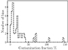 |
Fig. 7. Distribution of the estimated background AGN contamination fraction in the SFR-M⋆-D stack bin in our sample. The contamination fraction assuming the eRASS1 flux sensitivity limit of each individual galaxy. The median value of the distribution is 17%. The total surface of the 5 stacks with contamination fraction higher than 50% is significantly higher than all the rest used in our analysis resulting in an overestimation of the background AGN contamination. |
In addition, we calculated the mean LX of the stacks in the 0.5–2 keV band, assuming the median distance of the galaxies in each SFR-M⋆-D bin. In Fig. 8 we plot the LX as a function of the mean SFR colour-coded with the contamination fraction. For comparison, we overplot the scaling relation from Mineo et al. (2014) (M14) after converting it to the adopted 0.5–2 keV band by using the conversion factor c3 (see Table 2). As it is shown the contamination is independent of the SFR-M⋆-D bins and there is no systematic trend with SFR or LX.
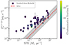 |
Fig. 8. X-ray luminosity (0.5–2 keV) as a function of the SFR for the stacked data with reliable flux measurements colour-coded with the estimated contamination by the background AGN. Only the stacks with available estimation of the background contamination are shown. For comparison, we overplot the scaling relation from Mineo et al. (2014) (M14). We see that the contamination is independent of the SFR-M⋆-D bins and there is no systematic trend with SFR or LX. The few stacks with very high contamination fraction (> 50%) are due to their total surface which is systematically higher than all the rest used in our analysis resulting in an overestimation of the background AGN contamination. |
For very few bins (i.e. five) the contamination fraction is higher than 50%. This could be due to two reasons. The first is because the galaxies that contribute to these stacks have large angular sizes increasing the total surface and consequently the calculated background AGN contamination is overestimated. Indeed the total surface of these 5 stacks is significantly higher than all the rest that are used in our analysis. The second is the lack of strong XRBs populations in the galaxies that are included in these bins (their vast majority have no reliable flux measurements) resulting in a measured flux that is almost equal to or lower than the expected flux from background interlopers. This also explains the stacks that have > 100% AGN contamination. However, these statistical fluctuations for a small sub-population of galaxies do not change the main conclusion that the median AGN contamination of our final sample is negligible.
6. Results
6.1. eRASS1 sensitivity
The all-sky nature of the eRASS1 survey, as opposed to the other local galaxy surveys, allows us to study for the first time a completely blind and statistically significant sample of normal galaxies as a function of their stellar population parameters. In Fig. 9 we present the measured X-ray luminosity of the HEC-eR1 star-forming galaxies as a function of their distance in comparison with previous normal galaxy surveys (Mineo et al. 2014, orange triangles; and Vulic et al. 2022, lightseagreen stars).
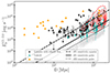 |
Fig. 9. LX versus D for the HEC-eR1 sample of star-forming galaxies. Black stars show the galaxies with reliable flux measurements and lightgray down-arrows, galaxies with uncertain flux measurements. For comparison, we also overplot the normal galaxies from Mineo et al. (2014) and Vulic et al. (2022) as orange triangles and turquoise stars. We also overplot with red contours the galaxy population expected to be observed in the eRASS:8 survey based on the simulation study of Basu-Zych et al. (2020). The dashed and solid lines mark the eRASS1 sensitivity limits at the ecliptic equator and poles respectively. The dotted line indicate the deepest sensitivity of the eROSITA survey which is expected to be reached at the poles of the eRASS:8. These lines are based on the sensitivity values reported in Predehl et al. (2021). |
As expected, the HEC-eR1 star-forming galaxies with reliable fluxes are consistent with the eRASS1 sensitivity limits at the ecliptic equator and poles ( and
and  respectively; Predehl et al. 2021). When we compare our sample with the previous study of nearby galaxies from Mineo et al. (2014), we find that the HEC-eR1 galaxy sample probes an unexplored region of the LX-D parameter space, that has not been studied before due to the limitations of the current and past observatories. The eRASS1 sample allows us to probe star-forming galaxies at luminosities as low as 1039 erg s−1 out to distances of ∼70 Mpc, and luminosities of as 1040 erg s−1 out to distances of ∼200 Mpc. Given the sensitivity of the eRASS1 survey we would expect to detect all the galaxies from Mineo et al. (2014) sample. However, because a large fraction of the latter galaxies, especially at very small distances, fall outside the west hemisphere of the sky they are not covered by eRASS1. The comparison with the results from the eFEDS survey (Vulic et al. 2022) shows that with the full depth eRASS:8 survey, we will be able to reach X-ray luminosities of typical dwarf galaxies, such as those observed in the very local Universe, out to ∼200 Mpc. The results from the eRASS1 survey are generally consistent with the simulation study of Basu-Zych et al. (2020), who predicted the populations expected in the complete eRASS:8 survey (red contours), especially considering that this simulation is based on pre-launch sensitivities and detector background.
Since we are interested in the scaling relation between the X-ray luminosity and the SFR, it is informative to explore the eRASS1 sensitivity on the LX-SFR plane for the HEC-eR1 galaxy sample. To that end, we utilize the SFR-M⋆-D binning scheme presented at Sect. 5.2, along with the eSASS sensitivity maps which provide the limiting flux given the local background and exposure time at the location of each galaxy. For each bin, we calculated the limiting luminosity (in the 0.5–2 keV energy band), based on the average limiting flux and median distance of the galaxies. This gives us an indicative minimum luminosity above which we can detect point sources in each SFR-M⋆-D bin. The sensitivity for the sample galaxies depends on their angular size but nonetheless, these lines give us an indication of the eRASS1 survey. However, the sensitivity calculated for the individual objects is expected to tend towards the indicative value calculated with the above method for the more distant galaxies.
In Fig. 10, we present the result of this analysis, in the LX-SFR plane. The coloured lines correspond to the limiting LX in each SFR-M⋆-D bin, colour-coded by the median distance. Stars and grey down-arrows show the HEC-eR1 star-forming galaxies with reliable and uncertain flux measurements, respectively. The red dashed line corresponds to the standard LX-SFR scaling relation from Mineo et al. (2014) along with the 1σ scatter.
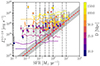 |
Fig. 10. LX versus SFR for the HEC-eR1 sample of star-forming galaxies. Black stars show the galaxies with reliable flux measurements and lightgray down-arrows galaxies with uncertain flux measurements. The lines correspond to the limiting LX in each SFR-MD bin, colour-coded by their median distance. Vertical black dashed lines indicate the SFR bins presented in Table 5. The red dashed line shows the standard LX-SFR scaling relation from Mineo et al. (2014) along with the 1σ scatter. |
As it is shown, all the HEC-eR1 star-forming galaxies with reliable fluxes are above the sensitivity limit of the eRASS1 survey. This plot also indicates that in the very local Universe (≲10 Mpc) the galaxies with reliable flux measurements are at least ∼1 dex above the sensitivity limit of ∼1038 erg s−1, while at larger distances we are sensitive to systematically high-luminosity galaxies. However, by including the constraints on the luminosity for the unreliable measurements (grey points) we remedy this bias.
6.2. Hot gas contribution
It is well known that the integrated X-ray emission of star-forming galaxies is partly due to the diffuse X-ray emission of hot-ionised gas (with temperature ∼0.5–1.5 keV) (Mineo et al. 2012a; Lehmer et al. 2022). This hot gas is the result of the cumulative effect of strong winds from massive stars and supernovae (SNe) and it is correlated with regions of recent star formation (see Fabbiano 2019, for a review).
Our best-fit results obtained from the spectral analysis in Sect. 5.1 suggest that the temperature of the hot gas is kT = 0.70 keV which is in excellent agreement (in the band that we measured the spectrum; 0.6–2.3 keV) with the stronger hot gas components of Mineo et al. (2012b) and Lehmer et al. (2022), who calculated kT = 0.67 keV, and kT = 0.70 keV, respectively. By using the best-fit model, we calculated the flux of the total (XRB+hot gas) component ( ) and the flux of the thermal component (
 ). The average hot gas contribution is
 (5)
(5)
As a result, the average diffuse X-ray emission of the HEC-eR1 star-forming galaxies, is only a small fraction of the total average integrated flux, indicating that the measured X-ray emission is dominated by a power-law component associated with XRBs.
6.3. Scaling relations derived from the eRASS1 galaxy sample
In Fig. 11 we present the correlation between the integrated X-ray luminosity and the stellar population parameters of the star-forming galaxies for the HEC-eR1 sample. In the left panel, we plot the integrated LX in the 0.5–2 keV energy band as a function of the SFR. The right panel shows the LX per SFR in the 0.5–2 keV energy band as a function of the sSFR. The black stars indicate the individual galaxies with reliable flux measurement and their corresponding uncertainties at the 68% C.I. of the flux distribution. The grey down arrows show the galaxies with uncertain flux measurements at the upper 90% C.I. For comparison, we overplot the scaling relations from Mineo et al. (2014) (M14) and Lehmer et al. (2016) (L16), respectively. The M14 scaling relation was converted from the reference 0.5–8 keV band to the adopetd 0.5–2 keV band, using the conversion factor c3 (see Table 2).
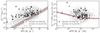 |
Fig. 11. Distribution of the LX0.5 − 2 as a function of the SFR and the sSFR. The left panel shows the distribution of all the HEC-eR1 secure star-forming galaxies in the |


We interestingly find that our population of star-forming galaxies shows elevated X-ray luminosity in comparison to the standard scaling relations of M14 and L16. The majority of galaxies with reliable flux measurements show systematically higher luminosities which can reach 1042 erg s−1. In particular, galaxies with SFR < 5 × 10⁻¹ M⊙ yr−1 exhibit significant excess from the standard scaling relations while this excess is decreasing as we go towards higher SFR regimes. In addition, a sub-population of very actively star-forming galaxies with sSFR > 10−10 M⊙ yr−1/M⊙ reaches very high X-ray luminosities per SFR, up to 1040 erg s−1/M⊙ yr−1.
We also see that although all the reliable galaxies are above the scaling relation, a significant fraction of the galaxies with uncertain fluxes has 90% upper confidence intervals well below the M14 best-fit line. This can be explained by the fact that eRASS1 is a flux-limited survey resulting only in the detection of the most X-ray luminous star-forming galaxies. However, even with this relatively shallow survey, we can set useful limits on the X-ray emission of galaxies below the expected scaling relations. The same behaviour is also observed in the LX/SFR-sSFR scaling relation. The vast majority of the star-forming galaxies with reliable measurements show a significant excess from the L16 relation while the galaxies with uncertain flux measurements are symmetrically distributed along the L16 best-fit line.
From the figure, we also see that the scatter of the X-ray emission in our blind galaxy sample (including reliable and uncertain flux measurements) is significantly larger than the 1σ scatter from the best-fitted lines of M14 and L16. The high scatter is also confirmed by the two individual extremely luminous galaxies with LX/SFR > 1042 erg s−1 cm−2 /M⊙ yr−1 (PGC24071, PGC1133474). A detailed inspection of their X-ray and optical images revealed that they are clean of X-ray contaminants (e.g. background AGN etc.) implying that all the X-ray emission is produced by XRB populations with a small contribution of hot gas. While they follow the linear form of the L16 in the low-sSFR, their dispersion is much higher than the expected value.
6.4. Average scaling relations of the eRASS1 galaxy sample
In order to study the average X-ray luminosity of the HEC-eR1 star-forming galaxies and its connection with their stellar populations we used the results of the SFR-M⋆-D stacks (see Sect. 5.2). In Fig. 12 we present the distribution of the SFR-M⋆-D stacks in the LX-SFR and the LX/SFR-sSFR parameter space, respectively. The open blue squares indicate the stacks with reliable flux measurements and the blue down-arrows the stacks with uncertain flux measurements. For comparison, we overplot the population of individual galaxies following the same notation as in Fig. 11. The scaling relations from M14 and L16 are also plotted. The blue shaded region indicates the upper and lower 90% C.I. of the master posterior distribution of the X-ray luminosity per stack based on our bootstrapping analysis (see Sect. 5.3). As we see the stacked data are more symmetrically distributed and closer to the scaling relations than the individual galaxies. This is expected since the large number of individual galaxies with uncertain fluxes per bin tends to bring the stacks closer to the best-fit lines of M14 and L16, respectively. Based on the results of the bootstrap analysis, we see that the upper 68% C.I. of the master posterior X-ray luminosity is very close to the upper error of the actual measurement. This indicates that the high X-ray luminosities of the average population of galaxies are not driven by a few luminous individual sources.
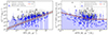 |
Fig. 12. Bootstraps distribution of the |


However, there is still an excess of our stacked data with reliable flux measurements (i.e. 58 stacks) from the M14 standard scaling relation, especially for the lower SFRs and the higher sSFRs. In order to quantify the average excess per SFR bin, in Fig. 13 we present the excess (in units of dex) from the M14 standard scaling relation (in the 0.5–2 keV energy band) as a function of SFR. The error bars were calculated based on the excess of the upper and lower 68% of the X-ray luminosity distribution from the reference relation. The light grey shaded region is the 1σ scatter around the M14 relation. As it is shown the average excess for a galaxy population within the SFR bin 0.001 − 0.01 M⊙ yr−1 is up to ∼ 2 dex while as the SFR increases the excess decreases. For the SFR bins 1−5 M⊙ yr−1, 5−10 M⊙ yr−1, and 10−30 M⊙ yr−1 the excess is consistent with the scaling relation.
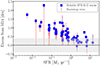 |
Fig. 13. Excess of the SFR-M⋆-D stacks with reliable flux measurements from the |

In addition, in Fig. 13 we also show with the red error bars the errors derived from the boostrap analysis. These are calculated based on the excess of the upper and lower 68% C.I. of the master X-ray posterior luminosity with respect to the M14 relation (see Sect. 5.3). This demonstrates that the observed excess is real and not due to strong statistical fluctuations of a sub-population of extreme X-ray luminous individual galaxies that dominates the stacked signal in each bin. Furthermore, the scatter of the stacked data seems to correlate with the SFR. For SFR > 3 × M⊙ yr−1 the stacks are consistent with the 1σ scatter of M14, while for lower SFRs the dispersion around the relation is increased. In Sect. 6.5 we quantify this SFR-dependent scatter by taking it into account during the fits of the scaling relations.
We find that both the individual HEC-eR1 star-forming galaxies and the stacked data per SFR-M⋆-D bins show significant excess from the standard scaling relations. This excess is very high and cannot be due to the background AGN contamination (∼10% of the total measured X-ray flux; see Sect. 5.4) or hot gas contribution (∼13% to the total X-ray flux; see Sect. 6.2). As a consequence, this excess can be the result of the effect of i) the gas-phase metallicity of the stellar populations (Fornasini et al. 2019), ii) the age of the stellar populations (Gilbertson et al. 2022), or iii) the stochastic sampling of the X-ray luminosity function (XLF) of XRBs (Lehmer et al. 2021). In Sect. 7 we discuss all these possible explanations in detail.
6.5. Fitting of the scaling relations
In order to study the connection between the integrated X-ray luminosity of HEC-eR1 star-forming galaxies with the SFR, M⋆, and metallicity, and to quantify the observed excess, we employed the maximum likelihood fitting methodology developed in Kouroumpatzakis et al. (2020). In contrast to other standard fitting techniques, this method utilizes the full probability distribution for the dependent and independent variables data which can be different for each data point and of any form even non-parametric. This is particularly important given the wide range of X-ray intensities in our sample which can be described neither by a Gaussian nor by a Poisson distribution (cf. van Dyk et al. 2001) given the very small number of counts and the non-negligible background. In addition, since the fit is performed on the posterior distribution, we can use the entire dataset including all the galaxies, even those with uncertain flux measurements, alleviating in this way the bias due to X-ray selection effects.
In our analysis, we simultaneously fitted the X-ray probability distributions as they were calculated in Sect. 3 for the stacked data per SFR-M⋆-D bin. This allows us to examine the scaling relation between X-ray luminosity and the parameters of stellar populations in terms of average statistical measures and with a higher signal-to-noise ratio than the individual galaxies.
6.5.1. LX-SFR-M⋆ scaling relations
Following previous works suggesting non-linear scaling of the X-ray luminosity and SFR (e.g. Lehmer et al. 2016, 2019; Kouroumpatzakis et al. 2020; Riccio et al. 2023) for the fit of the LX-SFR scaling relation, we used the following model:
 (6)
(6)
where A is the power-law slope and 10B is the LX/SFR scaling factor, and ϵ(log(SFR)) is an intrinsic scatter term in log LX that can depend on the SFR. Our results (see Fig. 11, Fig. 12) as well as previous studies (Lehmer et al. 2019; Kouroumpatzakis et al. 2020) indicate that the scatter in the LX-SFR scaling relation is anti-correlated with the SFR, especially in the lower SFR regimes. For this reason, the term ϵ(log(SFR)) is modelled as a Gaussian random variable with mean μ = 0 (i.e. around the best-fit line) and standard deviation σ = σ1logSFR + σ2. In particular, the intrinsic scatter due to the stochasticity (parameterised by σ1) was allowed to vary linearly with the log(SFR). The fit was performed using the Markov Chain Monte Carlo (MCMC) technique with uniform priors for the model parameters: A ∈ [0, 2], B∈ [36, 42], σ1 ∈ [ − 1, 2], and σ2 ∈ [0, 2]. We opted to use 100 walkers and 10 000 iterations in order to ensure the convergence of the fit.
In Table 6 we present the best-fit results on the stacked data per SFR-M⋆-D bin. We find that the slope is significantly sub-linear ( ) indicating that the correlation between the LX and the SFR is not just a simple one-to-one linear relation. In addition, the dependence of the intrinsic scatter on the SFR (parametrised as σ1) is significantly lower than zero (
 ). The best-fit value for the free parameter σ2 is
  .
.
Scaling relations best-fit results.
In the left panel of Fig. 14 we present the correlation between the X-ray luminosity and the SFR following the same notation as in Fig. 12 and our best-fit is shown with a black dashed line. The orange-shaded region indicates the 1σ SFR-dependent intrinsic scatter. For comparison, we also plot the LX-SFR scaling relations which are widely used in the literature. The red dashed line shows the standard scaling relation M14. The green dashed line indicates the relation from L16 who fitted a combined sample of normal local galaxies and stacked sub-samples of the ∼6 Ms Chandra Deep Field-South (CDF-S). In particular, we used their best global fit (Table 3) which is redshift-dependent and accounts for the contribution of the LMXBs. However, we considered only the HMXBs component. The reason for that is that our sample is dominated by pure star-forming galaxies and the contribution of LMXB populations is negligible (see right panel of Fig. 12, and Sect. 7.1). In addition, we assumed z = 0 given that our sample only includes galaxies within a distance of 200 Mpc. The brown-dashed line shows the LX-SFR scaling relation from Lehmer et al. (2019) (L19) who presented updated constraints based on the X-ray luminosity functions of XRB populations based on a sample of 38 nearby galaxies. Finally, the magenta dashed line indicates the recent scaling relation from Riccio et al. (2023) who fitted the LX-SFR relation in a sample of normal galaxies detected in the eFEDS. Because each work was performed in a different energy band we converted all of them in the adopted 0.5–2 keV band using the conversion factors from the Table 2.
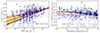 |
Fig. 14. Comparison of our best-fitted scaling relations with the previous works. The left panel shows the distribution of the SFR-M⋆-D stacks in the |


We find that our best-fit line confirms the correlation between the X-ray luminosity and the SFR of the average population of star-forming galaxies in each SFR-M⋆-D bin. This is in agreement with the results of the previous works. However, our relation is higher than almost all the other works, with a slightly shallower slope. This shallowness compared to the other scaling relations reflects the population of X-ray luminous galaxies, especially in the lower SFR regimes. Only the R23 scaling relation is higher than our best fit. The reason for that is that Riccio et al. (2023) worked only with the eFEDs detections tracing only the positive fluctuation of the XRBs populations. On the other hand, in our analysis, we considered all galaxies including those with uncertain flux measurements. We also find that the M14, L16, and L19 relations are consistent with each other.
We also find that the free parameter σ1 which traces the intrinsic scatter is negative. This indicates for the first time that the intrinsic scatter in the X-ray emission of the average population of star-forming galaxies anti-correlates with the SFRs. The effect of the SFR-dependent scatter is clearly shown for SFR < 2 M⊙ yr−1 where the expected X-ray luminosity from star-forming galaxies is strongly affected by the stochastic sampling of the XRBs X-ray Luminosity Function (XLF) of the galaxies. In addition, we see that ϵ(log(SFR)) = 0 for SFR > 2 M⊙ yr−1. This behaviour has no physical origin, but instead it is the result of the linear parametrisation of the ϵ(log(SFR)).
As opposed to the previous studies of local galaxies, the eR1-HEC star-forming galaxy analysis is completely blind to selection biases. This is because we also consider objects that are not formally detected in the eRASS1 survey. As a result, it is more representative of the X-ray properties of normal galaxies in the local Universe, indicating that the correlation between the integrated X-ray luminosity and the SFR is slightly different than the previous works which were limited to small galaxy samples.
Given that we are working with the integrated X-ray emission of each galaxy we have contributions from both HMXB and LMXB populations. In order to disentangle these two contributions we also performed a joint X-ray luminosity, SFR, and M⋆ maximum likelihood fit. Our model was of the form
 (7)
(7)
where the free parameters A, and B trace the young stellar populations (associated with HMXBs) and the old stellar populations (associated with LMXBs), respectively. The term σ was used in order to account for the intrinsic scatter in the data.
However, the results of this fit were strongly unconstrained because as it is seen in the right panel of Fig. 12, our stacks are underpopulated in the low sSFR regime (sSFR < 2 × 10⁻¹⁰ M⊙ yr−1/M⊙) where the LMXB populations start to contribute significantly. Furthermore, the majority of these stacks did not yield reliable X-ray measurements. This indicates that our sample is dominated by pure star-forming galaxies. This is also confirmed by our analysis in Sect. 7.1 which shows that the contribution of the LMXBs to the observed X-ray luminosity excess is negligible for the majority of the stacks. As a consequence, the fitted X-ray luminosity scaling relation does not require any additional LMXB component at a statistically significant level. For that reason our sample does not allow us to make any conclusive statement about the correlation between the X-ray luminosity, SFR, and the M⋆.
In order to explore the effect of the M⋆ in introducing scatter and driving the observed excess we repeated the stacking process in SFR-D bins (i.e. ignoring any dependence on the M⋆). This results in a tighter LX-SFR relation, as expected, but with still a flatter slope than the standard scaling relations. This indicates that stacking all available bins at low SFR does not bring the average X-ray luminosity to consistency with the standard relation, indicating that the excess is not an artefact of the binning scheme.
6.5.2. LX-SFR-metallicity scaling relation
Several studies (e.g. Fornasini et al. 2019; Brorby et al. 2016; Vulic et al. 2022) have shown that LX/SFR tends to be elevated in star-forming galaxies with lower-metallicity. Given that our sample spans about 1 dex in metallicity from 8.0 subsolar to 9.0 super-solar, we can study the LX-SFR-metallicity scaling relation for a wide range of the parameter space. In contrast to the observed log LX scatter dependence on the SFR (Sect. 6.5.1), in the right panel of Fig. 14 we see that the log LX scatter of our stacked data does not depend on the metallicity, since it remains constant across the entire metallicity range. Therefore, we considered a model with a fixed scatter that does not depend on metallicity:
 (8)
(8)
where Z is the metallicity in solar units calculated from the log(O/H) metallicity: Z = 10(log(O/H) + 12)−8.69 (adopting (log(O/H) + 12)⊙ = 8.69; Asplund et al. 2009). The A and 10B are the power-law of the non-linear metallicity dependence and the LX/SFR scaling factor, respectively. The fixed scatter term σ indicates a Gaussian random variable with μ = 0 and standard deviation σ. The fit was performed again using the MCMC technique assuming uniform priors for the model parameters A ∈ [ − 3, 1], B ∈ [39, 44], and σ ∈ [0, 5]. The number of walkers and iterations was 100 and 10 000, respectively.
The best-fit results are presented in Table 6. We find that the index is negative and sub-linear ( ) which is consistent with the results from previous works (e.g. Fornasini et al. 2019; Brorby et al. 2016; Vulic et al. 2022). In addition, we find that the fixed scatter of the LX/SFR is
  and is not correlated with the metallicity. In the right panel of Fig. 14 we present the best-fit line for the LX-SFR - metallicity relation (black dashed line) along with the metallicity-dependent scatter (orange shaded region). Following the same nomenclature as in Fig. 12, the blue squares and down arrows indicate the stacked data per SFR-M⋆-D bin. The black stars and the lightgray down arrows represent the individual HEC-eR1 galaxies with reliable and uncertain fluxes, respectively. For comparison, we overplot the empirical relations from a number of works. The dashed magenta line shows the best-fit line from a sample of 10 Lyman break analogs (LBAs), as presented by Brorby et al. (2016). The dashed brown line indicates the best-fit result from Fornasini et al. (2020) on stacked samples of galaxies spanning a redshift range z ≃ 0.1 − 0.9. In addition, the dashed darkgreen line indicates the best-fit line from Lehmer et al. (2021) who analysed Chandra data from 55 actively star-forming nearby (
 ) galaxies within a wide metallicity range 12+log(O/H) ≃ 7 − 9.2. For these works, we used the conversion factors c5, c6, and c7 (see Table 2), respectively, to convert the X-ray luminosity from their respective bands to the 0.5–2 keV band. Finally, with the cyan dashed line, we present the best-fit result from Vulic et al. (2022) who studied the LX/SFR – metallicity dependence for all the star-forming galaxies detected in the eFEDs field which reaches the full depth of eROSITA survey (eROSITA:8). We also overlay the theoretical prediction from the XRB population synthesis best model from Fragos et al. (2013) (red dashed line). We find that our results are in general agreement with those works but they show higher X-ray luminosities. In Sect. 7.2 we further discuss these results in more detail and compare them with the current LX-SFR – metallicity scaling relations.
7. Discussion
7.1. Excess from the standard scaling relations
Our best-fit results from the SFR-M⋆-D stacks, as well as the distribution of the individual galaxies, indicate that the local galaxy population shows a significant excess from the standard scaling relations of M14 and L16. In addition, this excess anti-correlates with the SFR of the host galaxy confirming similar indications from previous studies which have been performed on much smaller galaxy samples (Lehmer et al. 2016; Kouroumpatzakis et al. 2020).
In order to assess the significance of this excess, in Fig. 15 we present the distribution of the 0.5–2 keV X-ray luminosity of the galaxies in the different SFR bins we considered. This plot can be seen as an alternative version of the LX-SFR relation (Fig. 12) where each subplot represents a vertical slice with respect to the SFR. In each subplot, the black solid lines indicate the  from individual galaxies with reliable flux measurements, and the light grey histogram the
  from individual galaxies with uncertain flux measurements. For the latter histograms, we used the upper 90% C.I. of the X-ray luminosity, and as the result, the actual value of the LX is definitely lower. The blue solid and dashed lines show the
  distribution for the stacks with reliable and uncertain flux measurements, respectively. The red dashed line, shows the expected LX from the M14 for the mean SFR of the galaxies in each bin, while the yellow shaded region indicates the 1σ scatter from the best-fit line of M14.
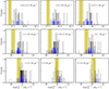 |
Fig. 15.
|

As we can see, the integrated X-ray luminosity of the individual HEC-eR1 star-forming galaxies is significantly elevated with respect to the expected X-ray luminosity for a given SFR. This excess is very strong in the low SFR regime (≲ 1 M⊙ yr−1) and it is decreasing towards higher SFRs. For the low SFRs the individual galaxies with reliable flux measurements reach very high X-ray luminosities up to typically ≳ 1042 erg s−1, well above the M14 scaling relation. On the other hand for high SFRs the X-ray luminosity of the individual galaxies is more consistent with the M14 scaling relation. We should note here that although the M14 relation is measured for galaxies down to SFR ∼ 0.1 M⊙ yr−1, Kouroumpatzakis et al. (2020) showed that it can be extended to lower SFRs.
Although the eRASS1 sensitivity limit does not allow us to measure precisely the flux for the majority of the galaxies in our sample, the distributions of the average luminosities of the stacks indicate a noteworthy trend. While many stacks are consistent or slightly above the standard scaling relation, we see that the upper 90% C.I. of the X-ray luminosity distribution of galaxies with uncertain flux measurements falls consistently well below the M14 scaling relation, specifically for SFR > 1 M⊙ yr−1. In particular, for the two highest SFR bins the distributions are almost symmetric around the scaling relation. This is the result of two factors: (i) the integrated X-ray luminosity is high enough to be detectable given the higher photon statistics of the stacks and their sensitivity limit (given their total exposure time and background), (ii) adequate sampling of the XRBs luminosity function since for these very highly star-forming galaxies stochastic effects are minimised, resulting in a large number of XRB populations with X-ray luminosities close to that expected based on the average scaling relation for a given SFR.
These results alongside the behaviour of the individual galaxies imply that: i) by taking into account the stacks with uncertain fluxes, the current scaling relation from M14 can describe well the correlation between the average X-ray luminosity and the average SFR of the HEC-eR1 star-forming galaxies for SFR > 0.5 M⊙ yr−1, ii) for ≪ 0.5 M⊙ yr−1 the measured average X-ray luminosity is much higher than expected from the M14 relation (Figs. 13, 14), and iii) the scaling relation proves inadequate in accurately describing the individual galaxies since it does not account for the much larger intrinsic scatter (Fig. 14).
Apart from the excess, another very interesting result in Fig. 15 is the increased scatter in comparison to the 1σ scatter of the M14 relation. In particular, we see an anti-correlation of the scatter of the HEC-eR1 star-forming galaxies with the SFR. This is clearly shown by the distribution of the X-ray luminosities of the individual galaxies around the scaling relation. As the SFR increases, the scatter decreases and the LX distribution of the individual galaxies with reliable or uncertain flux measurements becomes tighter and more consistent with the standard scaling relation. This is confirmed by the anti-correlation of the intrinsic scatter term with SFR in the scaling relation fits (Sect. 6.5.1).
A possible explanation for the increased excess and scatter could be the contamination by background AGNs within the D25 of the galaxies. However, our results in Sect. 5.4 suggest that the contamination in our sample is very low to significantly affect the measured fluxes and the corresponding luminosities, especially in the low SFR regimes.
Another source that potentially contributes to the integrated X-ray luminosity (and as a result to the measured X-ray luminosities) is the diffuse emission from hot-ionised gas. Lehmer et al. (2022) calculated the scaling relation between the hot gas luminosity and the SFR by analyzing Chandra observations of a sample of 30 very actively star-forming low-metallicity galaxies. By taking into account the effect of metallicity in the XRB component they fitted a global spectral model considering an absorbed power-law component corresponding to the XRB component, and two absorbed thermal plasma components of different temperatures. By using the best-fit parameters from this work (Table 3), we calculated the relative contribution of the HMXB and the hot gas components given the SFR of the galaxies in each stack. We found that the hot gas contribution is ∼32% in the 0.5–2 keV energy band, with the hot gas component being negligible above 2 keV. In addition, Mineo et al. (2012b) measured the hot gas emission from a sample of local galaxies which covered a broad range of SFR and M⋆ and they found that the X-ray luminosity of the hot gas correlates with the SFR as  in the 0.5–2 keV energy band. Furthermore, they found that the scaling relation for total X-ray luminosity (HMXBs + hot gas) and the SFR is
  in the 0.5–8 keV energy band. By using the conversion factor c3 from Table 2 we converted the scaling relation from the 0.5–8 keV band to 0.5–2 keV and we calculated that the hot gas contribution fraction is ∼30% of the total (HMXBs + hot gas) X-ray luminosity in the 0.5–2 keV energy band. In Sect. 6.2 we found that the hot gas contribution in the 0.5–2.0 keV band flux is ∼13%. This result corresponds to an X-ray luminosity excess of 0.05 dex which is not enough to explain the observed excess and the scatter that we see in our HEC-eR1 sample.
We see that our estimation of the hot gas contribution is much lower than that inferred from the analysis of Lehmer et al. (2022) and Mineo et al. (2012b). This difference is the result of sample selection. In particular, the galaxy sample of Lehmer et al. (2022) consists of dwarf star-forming galaxies in a narrower range of stellar mass ( ) and SFR (SFR ∼ 1−10 M⊙ yr−1), and much higher sSFRs (
 ) than the general population of star-forming galaxies (cf. Fig. 4). Furthermore, the sample of Mineo et al. (2012b) although well distributed on the main sequence plane is biased towards higher sSFRs
  . These systematically higher sSFRs of the galaxies used in these studies compared to our average galaxy sample, result in a stronger hot gas component, due to the intense star formation that results in the formation of more massive stars with strong winds and more supernovae (SNe). In fact when we apply the spectral model of Lehmer et al. (2022), and keeping fixed the column density of absorption components, the relative contributions of the two APEC components and their temperatures, as well as, the power-law photon index to their best-fit values, (in order to get a meaningful fit to our spectrum), we find that the total hot gas contribution for our galaxy sample is 20%, similar to our result in Sect. 6.2 (leaving free the power-law photon index results in slightly lower contribution of ∼15%). This result implies that the difference in the hot gas contribution between the previous works and our work, is due to the different properties of the galaxy samples considered. On top of that, all the previous works on the X-ray emission of nearby star-forming galaxies are affected by the observation bias since they were focused on well-known galaxies lacking a complete coverage of the overall population of star-forming galaxies.
Recently, Laktionov et al. (in prep.), studied the diffuse X-ray emission from a representative and, well distributed in the main sequence plane, sample of 74 nearby galaxies (D < 17 Mpc), using data from the eRASS:4. In particular, they divided their galaxy sample into 3 different SFR bins (SFR < 0.1 M⊙ yr−1, 0.1 M⊙ yr−1 < SFR < 1 M⊙ yr−1, and SFR > 1 M⊙ yr−1) and using the corresponding stacked X-ray spectra they calculated the average hot gas contribution to the total X-ray (hot gas+XRB) flux in each SFR bin. Their analysis showed that in the lower and medium SFR bins (i.e. SFR < 0.1 M⊙ yr−1, 0.1 M⊙ yr−1 < SFR < 1 M⊙ yr−1) the hot gas contribution in the 0.5–2 keV band is 19% and 29%, respectively. This result is lower than the contribution estimated in the Mineo et al. (2012b) and Lehmer et al. (2022) works, in reasonable agreement with our estimation of (∼12%; 0.5–2 keV), especially in the low SFR regime where the excess is strongest. This relatively low hot gas contribution towards lower SFR bins also indicates that the origin of the observed excess in the lower SFR regimes is not due to contamination of diffuse emission in the integrated flux we measure. For their highest SFR bin (SFR > 1 M⊙ yr−1) the hot gas contribution increases (∼38%) which is expected due to more intense star-forming activity in these galaxies. However, the excess we measure is not observed at these high SFRs (Fig. 11) but in lower SFR (< 1 M⊙ yr−1) where the hot gas contribution is much smaller.
X-ray emission originating from LMXBs is another potential contributor to the overall integrated emission of galaxies. More specifically, the X-ray emission produced by LMXB populations usually dominates the X-ray output of galaxies in the very low sSFR regimes (see Fabbiano 2019, and references there in). Given that our sample of galaxies reaches SFR as low as ∼ 10−3 M⊙ yr−1 and sSFR values around sSFR it is possible that the observed excess is due to emission from LMXB populations.
In order to estimate the contribution of the LMXB populations, we calculated the total luminosity by integrating their X-ray luminosity function (XLF):
 (9)
(9)
We adopted the XLF of Lehmer et al. (2019) (Eq. (2)) who parameterised it with a broken power-law and by using the best-fit parameters given in their Table 4 (column 6) we calculated the expected total 0.5–8 keV X-ray luminosity from LMXBs for a given M⋆. As low limit in the integration, we assumed Lmin = 1036 erg s−1 and for Lc we used the value Lc = 5 × 1040 erg s−1. Using the conversion factor c4 (see Table 2) we converted the X-ray luminosity from the 0.5–8 keV energy band to the 0.5–2 keV band adopted in this work. Then the LMXB contribution is
 (10)
(10)
where  is the expected luminosity based on the XLF of LMXBs and L0.5 − 2 is the measured integrated X-ray luminosity.
We performed the calculation for both, the individual galaxies and the SFR-M⋆-D stacks with reliable flux measurements. In this way, we can estimate the impact of the LMXB populations on the observed excess on a galaxy by galaxy basis, as well as on the average galaxy population per SFR-M⋆-D bin. In Fig. 16 we plot the percentage of LMXB contribution as a function of the SFR and the sSFR, respectively. The grey stars represent the individual galaxies with reliable flux measurements and the colour-coded squares the reliable stacks. The colour-code indicates the logarithm of the number of galaxies that participate in each SFR-M⋆-D bin. The error bars were calculated assuming the lower and upper 68% C.I. of the X-ray luminosity distribution for each measurement. We see that for both populations (individual galaxies, and stacks) the LMXB contribution fraction is negligible (< 10%) for the low SFRs and it is slightly increased (∼ a factor of 3) for higher SFR values. This result implies that the excess of up to ∼ 2 dex in galaxy populations with SFR < 0.1 M⊙ yr−1 (see Fig. 13) cannot be attributed to emission from LMXB populations. In addition, we find that the LMXB contribution anti-correlates with the sSFR as it is expected from the connection of the LMXBs with the old stellar populations of the host galaxy. Contrary to our expectations, a few stacks in the SFR > 0.3 M⊙ yr−1 regime appear to have higher LMXB contribution (> 40%) than the rest of the stacks. This unexpected behaviour can be explained by the limitations introduced by the definition of the SFR-M⋆ grid and the eRASS1 sensitivity limit. In particular, as shown in Fig. 6, the asymmetry in the SFR-M⋆ bins results in wider M⋆ bins, especially in the two ends of the M⋆ distribution. As a consequence, the computed mean M⋆ is biased towards higher stellar masses than the average mass of the galaxies for these bins, resulting in a higher expected LX due to LMXB populations and hence a larger inferred LMXB contribution fraction. This bias is also strengthened by the systematically smaller number of individual galaxies within these particular bins (colour-code in Fig. 16), which introduces larger statistical fluctuations in the calculation of the mean M⋆. In addition, the small number of galaxies participating in these particular bins, coupled with the fact that the measured fluxes for the majority of them are upper limits (since they are systematically in higher distances), results in larger uncertainties in the calculation of the integrated luminosity for the most distant bins which is translated in systematically larger uncertainties for the LMXB contribution fraction, for these specific stacks (as demonstrated by the larger error-bars in Fig. 16).
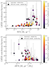 |
Fig. 16. Percentage of LMXB contribution as a function of the SFR (top panel) and the sSFR (bottom panel), respectively. The grey stars represent the individual galaxies with reliable flux measurements and the squares the reliable stacks. The colour-code indicates the logarithm of the number of galaxies that participate in each SFR-M⋆-D stack. The error bars were calculated assuming the lower and upper 68% C.I. of the X-ray luminosity distribution. |
It is clear from this analysis that the substantial excess and the large scatter, indicated by our findings, cannot be the result of contamination by background sources, contribution of hot gas emission, or the presence of LMXB populations. This suggests that the observed behaviour is likely influenced by either the characteristics of the host galaxies’ stellar populations, such as metallicity and stellar population age, or the inherent stochastic sampling of the HMXB XLF. In the next sections, we discuss in detail these factors and their role in the observed excess and dispersion in relation to the standard scaling relations.
7.2. Metallicity dependence
It is well known from previous studies (e.g. Basu-Zych et al. 2013; Fornasini et al. 2019; Lehmer et al. 2021; Vulic et al. 2022) that the integrated X-ray emission produced by HMXB populations is strongly correlated with the gas-phase metallicity of star-forming galaxies. In particular, it has been found that the LX/SFR tends to be elevated in galaxies with lower metallicity when compared to those with nearly solar metallicity. Moreover, it has been established that lower metallicity plays a significant role in the observed scatter of the LX-SFR scaling relation in the lower SFR regimes (Kouroumpatzakis et al. 2020, 2021; Vulic et al. 2022). These results also extend to higher redshift galaxies indicating that metallicity is responsible for the redshift evolution of HMXBs (e.g. Basu-Zych et al. 2013; Fornasini et al. 2019, 2020). The observational constraints from the previous works are in general agreement with the theoretical predictions from binary population synthesis models which suggest that the observed LX excess and scatter are driven by the metallicity (Fragos et al. 2013; Madau & Fragos 2017). This LX-SFR-metallicity dependence arises from the fact that lower metallicity stellar populations are expected to have relatively weak stellar winds resulting in less angular momentum loss from the binary systems and hence tighter orbits. Consequently, more Roche lobe overflow systems are formed resulting in higher accretion rates and thus in higher LX/SFR (e.g. Linden et al. 2010).
Given that our galaxy sample spans a metallicity range from sub-solar (down to [log(O/H)+12]∼8) to super-solar (up to [log(O/H)+12]∼9), in Sect. 6.5.2 we fitted the LX-SFR-metallicity relation to the stacked HEC-eR1 galaxy data per SFR-M⋆-D. In the right panel of Fig. 14 we present our best-fit result (black dashed line) in the form of LX/SFR as a function of the gas-phase metallicity. The shaded orange region shows the 1σ intrinsic LX metallicity-dependent scatter.
We see that our best-fit line follows well the distribution of the stacked star-forming HEC-eR1 sample of galaxies confirming the anti-correlation between the gas-phase metallicity and the LX/SFR. As the metallicity of the host galaxy decreases, its total X-ray output increases, in agreement with the theoretical predictions and the previous observational results. Both our dataset of individual galaxies and the stacked data with reliable flux measurements (depicted as black stars and blue open squares, respectively) exhibit an excess of ∼ 2.5 dex above the best-fit lines established by Brorby et al. (2016), Fornasini et al. (2019), and Lehmer et al. (2021). This is confirmed by our best-fit line which is higher than the current scalings relation by ∼0.5 dex, indicating once again the effect of a previous overlooked population of X-ray luminous galaxies, particularly in lower metallicities. Interestingly, we find that the best-fit line for the individual galaxies detected in Vulic et al. (2022) is higher than our line (which represents the average population of galaxies, including stacks with reliable and uncertain flux). This is expected given the higher sensitivity limit of the eFEDs survey (eight times deeper than eRASS1), and the fact that Vulic et al. (2022) used only X-ray detections without taking into account upper limits. On the other hand, Vulic et al. (2022) lacks the exceedingly X-ray luminous galaxies detected in the eRASS1 survey because of the large difference in the area between the two surveys, which does not allow the detection of rare objects within the 140 deg2 region covered by the eFEDs survey.
As discussed earlier, lower metallicity galaxies are more likely to produce X-ray luminous sources. In addition, lower-SFR galaxies, which are more sensitive to stochastic effects, also tend to have lower metallicities. The combination of these two effects results in the observed increase of the excess towards to lower metallicities. A quantitative analysis of the role of stochastic sampling as well as, the stellar population age, on the observed excess is presented in the following sections.
7.3. Stellar age dependence
Besides the effect of metallicity in the observed X-ray luminosity excess (see Sect. 7.2) another possible factor that contributes to the enhanced integrated X-ray luminosity of a star-forming galaxy, is the age of its stellar populations. Theoretical predictions of XRB population synthesis models (e.g. Fragos et al. 2013) show that the X-ray emission of an XRB population is higher at very young ages (< 20 Myr), gradually declining up to ∼ 100 Myr. This age dependence is also confirmed by a number of recent observational studies (Antoniou & Zezas 2016; Lehmer et al. 2017; Antoniou et al. 2019; Gilbertson et al. 2022).
In order to test the role of stellar population age in the enhanced X-ray emission of some of the SFR-M⋆-D bins used in our stacking analysis we performed the following analysis. We obtained He I 5876 and H[[INLINE925]] 6563 flux measurements by cross-matching the spectroscopically confirmed star-forming galaxies of the eRASS1 sample with the MPE-JHU DR8 galaxy catalogue (based on the SPECOBJID) which provides stellar continuum subtracted emission-line measurements. This resulted in a sample of 13 126 galaxies with available He I 5876 and H[[INLINE926]] flux measurements. We then calculated the ratio  for the galaxies with H α S/N ratio > 5, and He I 5876 S/N ratio > 3 (8287 galaxies). The different S/N thresholds were chosen in order to maximize the sample size with available measurements given the weakness of the He I 5876 line. For the remaining 4837 galaxies with He I 5876 S/N ratio < 3 we set the
  . In this way, we can quantify the relative contribution of the different age stellar populations in each galaxy. Higher flux ratios indicate stronger contribution of very young stellar populations (≲ 8 Myr) in the ionizing emission. On the other hand, when the ratio is close to zero, older (∼ 30 Myr) stellar populations dominate.
The exact age dependence depends strongly on the stellar evolution models assumed and especially the role of stripped stars (e.g. Götberg et al. 2020). Nonetheless, the He I lines trace younger stellar population than the Balmer lines. While XRB populations may also produce strong ionizing radiation, Garofali et al. (2024) showed that the contribution of XRBs in the ionisation of the He I 5876 line is negligible, indicating that this line is only due to the ionised gas around very young stellar populations and hence is a good age tracer.
In order to connect this age information with the average X-ray luminosity of the galaxy population in our sample, we calculated the median  of the individual galaxies participating in each SFR-M⋆-D bin. This resulted in 189 out of 239 bins with available measurements for
  . The remaining 50 bins did not include any galaxies with He I and H α measurements so we did not consider them in our analysis. In Fig. 17 we show the distribution of the SFR-M⋆-D stacks in the LX-SFR and the LX/SFR-sSFR plane, respectively. The stacks are colour-coded with the median
  . The open blue squares and the blue down-arrows indicate the stacks for which He I and H α emission line measurements were not available. For comparison, we overplot the scaling relations from M14 and L16.
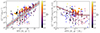 |
Fig. 17. Distribution of the |


As we see there is a clear correlation of the elevated X-ray luminosity with the median  of the stellar populations in each SFR-M⋆-D bin. For a given SFR the ratio increases towards higher LX (including the bins with uncertain luminosities which show systematically lower
  ratios). In particular, in the lower SFR regime (< 1 M⊙ yr−1) where the excess from the M14 scaling relation (Fig. 13) and the scatter are larger, the gradient of the
  ratio for the same SFR is stronger. This indicates that the stacks with high LX include galaxies hosting younger stellar populations (≲ 8 Myr) compared to stacks with lower LX which tend to include older stellar populations (< 30 Myr). For higher SFRs the effect of age is not so strong, and the gradient in the
  ratio is weaker. This is expected since at these high SFRs the stellar populations of these galaxies are unlikely to be dominated by short-duration very recent (≲ 10 Myr) star-formation bursts. Instead, they tend to be dominated by longer star-forming episodes, reducing the effect of strong age or metallicity variations in their X-ray output and subsequently the observed scatter and deviation from the average scaling relations.
These results are also confirmed by the trends in the LX/SFR-sSFR plane. For a given sSFR the ratio of the age tracers increases towards higher LX/SFR indicating that the average population of galaxies participating in those SFR-M⋆-D bins is dominated by younger stellar populations. On the other hand, stacks with lower sSFRs show systematically lower  ratio. This is normal since for the galaxies with less active star formation, we expect that the HMXB populations will be correlated with slightly older stellar populations that will fall in the age window traced by the H α, and their emission in the He I will be weak.
In order to address the combined effect of age and metallicity, in Fig. 18 we present the X-ray luminosity in the 0.5–2 keV band normalised by the SFR as a function of the gas-phase metallicity, colour-coded with the median  ratio. The metallicity and the SFR values of the stacked data correspond to the median and the mean values of the galaxy population included in each SFR-M⋆-D bin, respectively. We see that the increased LX/SFR towards subsolar metallicities is also correlated with an increase in the median
  ratio. This is generally expected since lower metallicity star-forming galaxies tend to be dwarf galaxies dominated by recent star-formation episodes. However, we also see that for a given metallicity the gradient in the
  increases towards higher LX/SFR implying that the age of the stellar populations plays a significant role in the observed LX excess and scatter. This gradient is significantly decreased (for solar or super-solar metallicity) and the LX/SFR we measured shows smaller deviations from the scaling relations. Furthermore, the scatter is also decreased.
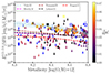 |
Fig. 18.
|

The results of Fig. 17 and Fig. 18 indicate that both metallicity and age of the stellar populations of the average galaxy population in each SFR-M⋆-D bin are highly correlated with the X-ray luminosity excess from the standard scaling relations of M14 and L16. However, based on this qualitative analysis we cannot conclude which of them shows a stronger correlation.
In order to assess the relative importance of the metallicity and stellar population age in driving the X-ray luminosity excess, we used the generalisation of the partial Kendal-τ coefficient for censored data (Akritas & Siebert 1996). The presence of a significant number of stacks with upper limits (especially in the low-luminosity bins; Fig. 17) requires the use of survival analysis methods in order to obtain unbiased results. We calculated the partial Kendal-τ coefficient for the measured excess of the LX/SFR with respect to the L16 and the M14 scaling relations, against the metallicity and the  ratio of each SFR-M⋆-D bin. We find that for both reference scaling relations, the null hypothesis for no partial correlation when the independent variable is the metallicity and the test variable is the
  ratio cannot be rejected. On the other hand, when the independent variable is the
  ratio (and the test variable is the metallicity) the zero partial correlation null hypothesis is rejected at the 5% confidence level. This indicates that the primary driver for the excess is the age of the stellar populations rather than the metallicity, in agreement with the qualitative picture seen in Fig. 18. This is also in agreement with the theoretical models of Fragos et al. (2013) which show that at the youngest ages (≲10 − 20 Myr) there is stronger evolution of the X-ray output of a stellar population as a function of the stellar population age than the metallicity.
7.4. Stochasticity effect
In Sect. 7.1 we showed that the average HEC-eR1 star-forming galaxy population shows a significant (up to ∼2 dex) excess above the standard scaling relations from M14 and L16. As we discussed, this excess is the result of extremely luminous individual galaxies possibly due to lower metallicities (Sect. 7.2) and/or very young stellar populations (Sect. 7.3) hosted by these galaxies. However, a reasonable question that arises is whether this excess is the result of stochastic sampling of individual XRBs associated with the galaxies participating in each bin, and has no physical origin (e.g. Gilfanov et al. 2004).
To answer this question, we performed a simulation study by calculating the expected X-ray luminosity due to stochastic sampling of the HMXBs XLF, for a fiducial galaxy with SFR, M⋆ and metallicity representative for each SFR-M⋆ bin. We then compared the resulting luminosity distribution with the observed X-ray luminosity of the galaxies in each bin. In particular, by using the mean SFR, and the median gas-phase metallicity per SFR-M⋆ bin (see Table 5) we first calculated the expected number of HMXBs per SFR-M⋆ bin using the metallicity-dependent XLF from Lehmer et al. (2021) (L21):
 (11)
(11)
assuming their best-fit parameters, which are a function of metallicity (from their Table 2), limiting luminosity Lmin = 1036 erg s−1, and maximum luminosity Lmax = 5 × 1041 erg s−1. We note that changing the low integration limit had little effect on the final result. Then, by sampling from a Poisson distribution with a mean equal to the number of expected HMXBs calculated above, we produced 20 000 draws of the expected number of HMXBs:
 (12)
(12)
Then we sampled the HMXB XLF, by drawing  sources each time. The total X-ray luminosity of the overall XRB population for each of the 20 000 draws is given by
 (13)
(13)
where  is the luminosity for each source drawn from the XLF for each instance. This is akin to simulating the X-ray emission of 20 000 galaxies with the typical properties of the galaxies in each SFR-M⋆ bin while accounting for fluctuations on the number of sources in each simulated galaxy, as well as, stochastic effects on sampling their XLF. For each of these distributions, we calculated the mean and mode and the 68%, 90%, 99%, and the 99.9% upper and lower C.Is. Since the XLF from Lehmer et al. (2021) is given in the 0.5–8.0 keV energy band we converted all the derived luminosities in our adopted band (0.5–2 keV) by using the conversion factor c7 from Table 2. For comparison, we repeated the analysis above by integrating the HMXBs XLF from Mineo et al. (2012a) for each SFR-M⋆ bin, in the same integration limits [Lmin, Lmax]. We converted again the X-ray luminosities from their 0.5–8 keV energy band to 0.5–2 keV using the corresponding conversion factor c8 from Table 2.
In Fig. 19 we present the distribution of the total expected X-ray luminosity (0.5–2 keV) due to the stochastic sampling of the HMXBs XLF from L21, as a function of the SFR. Orange and yellow shaded regions indicate the 90%, and the 99% C.I., respectively of the expected  distribution for each SFR-M⋆ bin. The magenta line shows the 99.9% C.I. of the same distribution and the red line the 99% C.I. from Mineo et al. (2012a) (M12). Brown open squares and blue stars show the mean and mode of the L21 distributions, respectively. The error bars around the mean correspond to the 68% C.I. Black stars (reliable flux) and grey down-arrows (uncertain flux) indicate the individual HEC-eR1 star-forming galaxies. The red dashed line shows the LX-SFR scaling relation from M14 with its 1σ scatter.
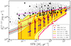 |
Fig. 19. Total expected X-ray luminosity (0.5–2 keV) due to the stochastic sampling of the HMXBs XLF from Lehmer et al. (2021) (L21), as a function of SFR. Orange and yellow shaded regions indicate the 99% and the 99.9% C.I. of the expected |

We see that the stochastic sampling of the HMXB XLF is not adequate to explain the most X-ray luminous individual galaxies in our sample. In particular, we find that a sub-population of galaxies has X-ray luminosities ∼1 dex higher than the upper 99.9% C.I. of the expected X-ray luminosity due to stochastic sampling. This population is spread in a SFR range of ∼ 0.01−2 M⊙ yr−1 and the majority of them has X-ray luminosity higher than 1041 erg s−1. These galaxies are strong outliers with respect to the average galaxy population in each SFR-M⋆ bin and the probability of stochastically observing them is lower than 0.05%.
We find that both, the L21 and M12 expected X-ray luminosity distributions for each SFR-M⋆ bin are narrower for high SFR values while they become broader going towards lower SFRs. This is expected because for higher SFRs we expect larger population of HMXB and as per the central limit theorem the sampling of their integrated X-ray emission converges to the mean of their expected value. On the other hand, for lower SFRs the sampling of the XLF tends to be more stochastic, and the expected total X-ray luminosity per SFR can be dominated by a few HMXBs drawn from the upper end of the XLF. In addition, we see that the mean values of the distributions are in excellent agreement with the LX-SFR scaling relation from Mineo et al. (2014) within the full SFR range. On the other hand, the mode values are in much lower luminosities for lower SFR values. This result implies that the previous studies tend to observe the most dominant X-ray luminous galaxies in the lower SFR regimes, lacking the bulk of the population of those galaxies. This underscores the need for blind galaxy surveys such as eRASS1 which can provide a less biased census of X-ray galaxies in the local Universe.
By comparing the upper 99% C.I.s of the expected  based on sampling from the M12 and L21 HMXBs XLFs, we find that for the latter we systematically sample more luminous HMXBs in the lower SFR regimes. This is due to the lower metallicity of the galaxies in those SFR (see Sect. 7.2) bins. The M12 XLF, does not take into account the effect of metallicity. However, the L21 XLF, which takes into account the metallicity, shows a flattening at the high luminosity end of the XLF for lower metallicities. In their work Lehmer et al. (2021) showed also that for super-solar metallicities the high-end of the XLF has a much steeper slope compared to the XLF for lower metallicities. This metallicity effect is clearly seen for
  where the mode and the mean values of the sampled distributions are systematically in slightly lower X-ray luminosities than those suggested from the M14 scaling relation. The galaxy sample from Mineo et al. (2014) includes mostly solar and/or sub-solar metallicity galaxies. On the other hand, our sample spans a range of solar and supersolar metallicities at these SFR regimes since it is more representative of the average galaxy population, resulting in steeper actual XLFs yielding HMBXs with lower X-ray luminosities. That explains why the mean and the mode values are below the M14 scaling relation for
  .
.
The analysis so far has assumed that the contribution of LMXBs is negligible. In order to address the role of LMXBs in the population of galaxies with significantly stronger X-ray emission with respect to the standard LX-SFR scaling relation in Fig. 20 we present the total expected LX/SFR distribution due to stochastic sampling of HMXBs XLF as a function of the sSFR. The diamonds indicate the mean LX/SFR per SFR-M⋆ bin, colour-coded with the gas phase metallicity. The sSFR and the metallicity were calculated using the mean SFR, M⋆, and the median gas-phase metallicity of the galaxies participated in each SFR-M⋆ bin. The orange and magenta lines correspond to the upper and lower 99%, and 99.9% C.Is. of the HMXBs expected LX/SFR, respectively. We also overplot with a red dashed line the LX/SFR – sSFR L16 scaling relation, and its corresponding 1σ scatter.
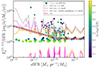 |
Fig. 20. Total expected LX/SFR distribution due to stochastic sampling of HMXBs XLF as a function of the sSFR. The rhombuses indicate the mean LX/SFR per SFR-M⋆ bin, colour-coded with the gas phase metallicity. The orange and magenta lines correspond to the upper and lower 99%, and 99.9% C.Is. of the HMXBs expected LX/SFR, respectively. Grey dashed line depicts the upper 99.9% C.I of the total expected luminosity accounting for the stochasticity of both, LMXBs and HMXBs. We also overplot with a red line the LX/SFR – sSFR L16 scaling relation, and its corresponding 1σ scatter. |
We see that the mean LX/SFR values from the stochastic sampling of the L21 XLF are in excellent agreement with the L16 scaling relation for sSFR > 10−10 M⊙ yr−1/M⊙ while for lower sSFRs the L16 scaling relation suggests an elevation of the LX/SFR because of the contribution of the LMXBs in these sSFR regimes. The LX/SFR from the L21 relation remains constant because their XLF accounts only for the HMXBs contribution. By calculating the difference between the expected mean LX/SFR per sSFR from the previous analysis and the LX/SFR suggested by the L16 we can estimate the contribution of LMXBs per sSFR. By adding this LMXB contribution to the upper 99.9% C.I of the X-ray luminosity due to the stochastic sampling of the HMXBs XLF, we can estimate the upper 99.9% C.I. of the total luminosity including both, LMXBs and HMXBs. This result is depicted by the grey dashed line. As we can see, for high sSFR values where the contribution of LMXBs is negligible the grey and the magenta lines are identical. On the other hand, for lower sSFRs the grey line is slightly higher than the magenta because the LMXBs have a stronger contribution to the X-ray output of the galaxies. Interestingly enough, we find that even accounting for the contribution of LMXBs on the stochastic sampling of LMXBs and HMXBs, the sub-population of galaxies (colour-coded stars) is still well above the upper 99.9% C.I. of the expected X-ray luminosity. This result indicates that their observed X-ray luminosities have a physical origin and they are not due to the stochasticity effect.
7.5. Low-luminosity AGNs or TDEs
Although our sample is carefully selected to exclude any potential contamination from AGN, the enhanced X-ray emission that we observe can be still due to the presence of a LLAGN in the central black hole of the host galaxy that is not traced by the optical and/or IR diagnostics we used.
To test this scenario we performed the following exercise. Assuming that the observed X-ray emission originates from accretion onto the supermassive black hole of the galaxy, we first calculated the black hole masses (MBH) of the HEC-eR1 galaxy sample with reliable flux measurements using the MBH-M⋆ scaling relation of Greene et al. (2020), which has a scatter of 0.65 dex. This calculation resulted in masses spanning a range of 103 − 108 M⊙ which includes the range of the Intermediate Mass Black Holes (IMBH) (Greene et al. 2020). Based on this black-hole mass, we calculated the bolometric Eddington luminosity
 (14)
(14)
and the corresponding Eddington fraction
 (15)
(15)
where  is the bolometric correction from the observed X-ray luminosity (
 ) based on the LLAGN SED of Ho (2008).
In Fig. 21 we present the distribution of our galaxy sample in the LX-SFR plane colour-coded with the Eddington fraction. Interestingly enough, we find that the most X-ray luminous galaxies ( ), as well as, the galaxies in the lower SFR regime which are responsible for the observed excess, have systematically higher Eddington fractions. These are very close to values typical for Seyfert 1 galaxies (∼10−4 − 10−1; Ho 2008). However, if the observed X-ray luminosities are from accretion on the central black hole at these Eddington limits, we would expect that their optical spectra would exhibit AGN signatures (e.g. broad and/or high-excitation spectral lines) unless the optical signature of the AGN is outshined by the optical emission produced by the star formation. To further investigate this scenario, we calculated the ratio of the observed Hα luminosity (
 ) to that expected assuming that the optical emission is from an LLAGN (
 ), using the LX/LHα ratio from the LLAGN SED of Ho (2008). Comparison of the observed Hα luminosity with that expected from the LLAGN, shows that the median
  /
/ is ∼4. For comparison, we performed the same analysis assuming the Seyfert SED from Ho (2008) which based on the derived Eddington fractions would be more appropriate. This resulted in a median
  /
/ is ∼2. This indicates that for some objects the emission from the LLAGN could be hidden by the star-forming component. However, a factor of approximately two to four is not very high, and if a fraction of the ionisation of the gas is due to the presence of a LLAGN, we should see its signature at least on the high-excitation spectral lines of their optical spectra, which would shift the galaxies in the locus of the composite objects in the BPT diagrams. Focusing on the most extreme X-ray luminous galaxies (
 ) of our sample, three of them have optical SDSS spectra (PGC1133474, PGC3441671, and PGC4340445; open black circles in Fig. 21). These (Fig. 22) are typical of star-forming galaxies without any AGN signature such as strong high excitation forbidden lines, or broad Balmer lines. In contrast, they are representative of the most typical optical spectra of star-forming galaxies, and in the case of PGC3441671, and PGC4340445 indicative of very young stellar populations. This is also supported by their location in the BPT diagrams. These results imply that although our galaxies have very high X-ray luminosities, which could be potentially produced by LLAGN, there is not any observable signature in their optical spectra. Of course, there might be an AGN contributing a smaller fraction of the X-ray emission but at the same time its role in the observed excess would be smaller.
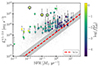 |
Fig. 21. LX-SFR distribution of the HEC-eR1 star-forming galaxies with reliable flux measurement colour-coded with the log( |

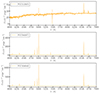 |
Fig. 22. Optical spectra of the most X-ray luminous ( |
Furthermore, given the large Eddington fractions and the small black-hole masses of these sources, we would expect that if they are powered by AGN they would exhibit strong variability. However, none of these galaxies is in the sample of X-ray emitting AGN selected on the basis of optical/UV/IR variability (Arcodia et al. 2024).
Recently Sacchi et al. (2024) presented a catalogue of 74 LLAGN detected in local (D ≲ 200 Mpc) dwarf galaxies (M⋆ ≲ 3 × 10⁹ M⊙) within the Western half of the eRASS1 survey. Out of these 74 galaxies, 17 have a match with our galaxy sample of eR1 star-forming galaxies, and for almost 50% of them their X-ray sources are likely off-nuclear. Although cosmological hydrodynamical simulations predict a population of off-nuclear AGN in dwarf galaxies (Bellovary et al. 2021), the presence of an off-nuclear X-ray source in a star-forming galaxy is also likely to be a ULX. In fact the lack of an unbiased census of ULXs using a blind galaxy sample, hampers the quantification of the off-nuclear AGN population.
Although the above analysis indicates that it is unlikely that the majority of the X-ray luminous galaxies we detect are due to LLAGN, a fraction of them may still be AGN with very weak optical signatures. Disentangling luminous XRBs from LLAGN is a very difficult task that requires good quality X-ray spectra and higher spatial resolution Chandra observations.
Another possible source of contamination may be the X-ray emission produced by Tidal Disruption Events (TED). If a star that is close to a supermassive black hole approaches the event horizon it can be disrupted, resulting in observed X-ray flares from tidal debris that falls back onto the black hole (for a review see; Gezari 2021). Recent studies have shown that TDEs are predominantly observed in post-starburst galaxies or galaxies that fall in the green valley in the colour-mass diagram (Law-Smith et al. 2017; van Velzen et al. 2021; Sazonov et al. 2021; Yao et al. 2023). However, given that our galaxy sample is composed of carefully selected star-forming galaxies, their vast majority falls well within the region of the main-sequence of star-forming galaxies (e.g. Peng et al. 2010). As a result, given the HEC-eR1 host galaxy properties, we would not expect strong contamination by TDEs. Sazonov et al. (2021) using X-ray data from the Russian half of the eRASS1 survey calculated a TDE rate of 1.1 × 10⁻⁵ galaxy−1 yr−1. However, since their galaxy sample is mostly comprised by post-starburst galaxies, it is not representative of the more actively star-forming galaxy population used in our work, and thus we cannot directly use it to estimate the expected TDEs in our sample. The most up-to-date measurement of TDE rates for star-forming galaxies (similar to those in our sample) and post-starburst galaxies (similar to those dominated the sample of Sazonov et al. 2021) is presented by Yao et al. (2023). Assuming that the ratio of the TDE rate derived in different wavelengths is independent of the galaxy type, we have
 (16)
(16)
where the left part of the equation gives the ratio of the optically and X-ray detected TDE rates in star-forming galaxies, and the right-hand side gives the same ratio for post-starburst galaxies. Using the values from Yao et al. (2023,  ,
,  ), and those reported in Sazonov et al. (2021), (
 ) we can calculate the X-ray based TDE rate for star-forming galaxies:
  . Based on this rate and the number of galaxies in our sample (18 790) we estimate that the TDE occurrence rate in our sample is 0.04 yr−1. Then using this mean value, and assuming a Poisson distribution, the probability of observing one or more TDEs within the 6-month eRASS1 scanning period is ∼ 0.98%, which is very low. As a result, we can conclude that the probability for our X-ray measurements to be contaminated by a TDE is very low, and that TDEs cannot explain the observed X-ray luminosity excess.
7.6. A population of extreme X-ray luminous starbursts
In Sect. 7.4, we showed that the stochastic sampling of the HMXBs XLF (accounting for the contribution of the LMXBs) is not adequate to explain the sub-population of the individual star-forming galaxies within the HEC-eR1 sample with extreme X-ray luminosities.
In order to evaluate the significance of this population of luminous galaxies we estimated their expected number based on the parent population of star-forming galaxies and the previously discussed stochasticity simulation for each SFR-M⋆ bin. The parent population in each bin consists of the HEC-eR1 star-forming galaxies which based on the sensitivity of the eRASS1 survey and their distance would be detectable beyond the 99.9% C.I of the expected X-ray luminosity distribution due to stochasticity ( ) for each corresponding bin. This is because only these galaxies would be potentially detected as outliers in our sample. This way we find that the number of outliers from this sample that would be detected above 99.9% C.I. by chance would be 0.05% of this parent sample.
In Fig. 23 we present the result of this analysis. Open orange squares and black stars indicate the number of the expected and the detected galaxies, respectively, with  per SFR bin. The error bars correspond to the
  , where N is the number of galaxies. We show only the results using the eRASS1 sensitivity at the poles as a conservative limit given the longer integration time resulting in higher sensitivity and larger number of galaxies. Surprisingly enough, we find that even in this deeper case the number of expected galaxies is zero. The fact that the expected number of galaxies per SFR bin with
  is zero, strengthens the argument that the sub-population of extreme X-ray luminous galaxies we find, is real and has an astrophysical origin. Although the significance of the detected galaxies compared to the expected is not very high for all the SFR bins, for some of them it is higher than 1σ. This marginal significance is expected given the shallowness of the eRASS1 survey. However, the significance of our findings will be increased substantially with the forthcoming deeper eRASS:4 and eRASS:8 surveys, which will increase the population of the detected galaxies.
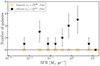 |
Fig. 23. Number of detected galaxies with |


Given that our findings suggest that this sub-population of HEC-eR1 star-forming galaxies has a physical origin, it is worth examining its stellar population properties. In Fig. 20 we see that it is mainly comprised of galaxies with higher sSFRs and lower metallicities. In particular, the vast majority of these galaxies span a sSFR range of ∼ 5 × 10⁻¹⁰ − 2 × 10⁻⁹ M⊙ yr−1/M⊙ and subsolar gas-metallicity in the range [log(O/H)+12] ∼ 8.1 − 8.6. In addition, these galaxies host systematically younger stellar populations (see Sect. 7.3). Given their higher sSFRs, their lower metallicities, and the age of their stellar populations, we can conclude that most likely these galaxies are experiencing a recent star-formation episode, which produces a larger number of luminous HMXBs resulting in an elevated LX/SFR comparing to the standard scaling relations. This result is also consistent with the work of Vulic et al. (2022) who detected in the eFEDS field a population of metal-poor dwarf starburst galaxies with similar characteristics as our population of galaxies.
This analysis reinforces the argument that large blind surveys can provide a more complete picture of the X-ray emitting galaxy population and their diversity. These intriguing results have important implications for understanding the population of XRBs contributing in the most X-ray luminous galaxies. This is particularly important for understanding the cosmological evolution of the galactic X-ray emission (e.g. as inferred from deep and wide area surveys (Lehmer et al. 2016; Aird et al. 2017; Fornasini et al. 2020) and their role in the preheating and reionisation in the early Universe. Stochasticity is particularly important for the latter since it will influence the shape of the cosmological 21 cm power spectrum (cf. Kaur et al. 2022). The next eRASS surveys will allow a clearer picture of this intriguing population of luminous galaxies to be obtained by providing more accurate measurements of their luminosity and setting better constrains on their overall scaling relations and scatter.
8. Summary and conclusions
In this work, we have presented the results of the first unbiased all-sky survey of star-forming galaxies with the eROSITA X-ray telescope. By combining the HECATE v2.0 value-added galaxy catalogue with the X-ray data obtained from the first complete eROSITA all-sky scan (eRASS1) and applying stringent optical and mid-infrared activity classification criteria, we constructed a sample of 18 790 bona fide star-forming galaxies (HEC-eR1 galaxy sample) with measurements of their integrated X-ray luminosity. This resulted in 77 star-forming galaxies with 3σ C.I. reliable X-ray fluxes, and 18 713 galaxies with uncertain flux measurements based on their posterior net count distribution. This sample probes star-forming galaxies at luminosities as low as 1039 erg s−1 out to distances of ∼70 Mpc and luminosities of 1040 erg s−1 out to distances of ∼200 Mpc. In this way, we have studied the relation between the X-ray emission of normal galaxies with their stellar population parameters (i.e. SFR, M⋆, metallicity, stellar population age) for the largest galaxy sample so far. Our main results are summarised as follows:
-
By stacking the X-ray spectra of all the galaxies in the HEC-eR1 sample, we derived the average X-ray spectrum of star-forming galaxies in the local Universe, which is well fitted by an XRB and a hot gas component (
 ,
,  ). Our best-fit results indicate that the average diffuse X-ray emission of the HEC-eR1 star-forming galaxies is 12.86%. This implies that only a small fraction of the total average integrated flux is due to hot gas, indicating that the measured X-ray emission is dominated by a power-law component associated with XRBs.
 -
We find that the integrated X-ray luminosity of the individual HEC-eR1 star-forming galaxies is significantly elevated (up to 1042 erg s−1) with respect to the expected X-ray luminosity from the standard scaling relations M14 and L16. This excess is stronger in the low SFR regime (≲ 1 M⊙ yr−1), and it decreases towards higher SFRs. Furthermore, the observed scatter (including reliable and uncertain flux measurements) is significantly larger than the 1σ scatter from the best-fit lines of M14 and L16.
-
By stacking the X-ray data in SFR-M⋆-D bins, we studied the correlation between the average X-ray luminosity and the average stellar population parameters. Although the distribution of the stacked data is closer to the scaling relations than the individual galaxies, we find that there is still an excess (reaching ∼2 dex at SFR ∼ 10−1 M⊙ yr−1) above the standard scaling relations that anti-correlates with the SFR. Bootstrap analysis showed that the observed excess is real and not due to strong statistical fluctuations of a sub-population of X-ray luminous individual galaxies that dominate the stacked signal in each bin.
-
This excess is not due to background AGN observed within the aperture of the sample galaxies or a population of LMXBs. The median AGN contamination fraction in our sample is 17%, and the LMXB contribution fraction is ≲10% for the low SFRs, while it is slightly larger for some of the higher SFR bins. It is also unlikely that LLAGN or TDEs, contribute significantly to the measured emission of the star-forming galaxies; however, the presence of LLAGN with weak optical signatures cannot be ruled out in some cases. Nevertheless, even if some LLAGN are present, it is unlikely that they drive the observed excess, especially in the low SFR regime, where luminous XRBs are expected.
-
Fits of the LX-SFR scaling relation, accounting for the intrinsic scatter, suggest that our relation is higher than almost all other works, with a slightly shallower slope, reflecting the population of X-ray luminous galaxies, especially in the lower SFR regimes. Furthermore, we find that the intrinsic scatter in the X-ray emission of the average population of star-forming galaxies anti-correlates with the SFR.
-
We find that the LX-SFR-metallicity scaling relation (spanning ∼1 dex in metallicity) confirms the anti-correlation of LX/SFR with the gas-phase metallicity also reported in previous works. However, our best-fit relation results in ∼0.5 dex higher X-ray luminosities than the current scaling relations due to the effect of a previously unrecognised population of X-ray luminous galaxies, particularly in lower metallicities.
-
We find that the stacks with higher X-ray luminosity tend to correlate more strongly with the
 ratio of the galaxies they contain than their metallicity. This indicates that the primary driver for the excess is the age of the stellar populations rather than the metallicity, and it is in agreement with the theoretical model of binary population synthesis models.
 -
Our results suggest that the stochastic sampling of the HMXBs XLF (accounting for the metallicity and the contribution of the LMXBs) is not adequate to explain the sub-population of individual star-forming galaxies with very high X-ray luminosities (up to ∼ 1041 erg s−1). This sub-population consists of star-forming galaxies with higher sSFRs, lower metallicities, and younger stellar populations. The younger age of the stellar populations is also confirmed by the optical spectra of some of the most X-ray luminous of them, which are typical of star-forming galaxies, indicating that they have experienced a recent star-formation episode and thus resulting in a larger number of luminous HMXBs and an elevated LX/SFR ratio.
These results demonstrate the power of large-area blind surveys in revealing rare populations of objects and recovering unbiased underlying correlations. The forthcoming eRASS surveys will provide a deeper census of the local galaxy populations and will help better constrain the correlation between X-ray luminosity, SFR-metallicity, and age in star-forming galaxies and their intrinsic scatter.
Bayesian Estimation of Hardness Ratios; http://hea-www.harvard.edu/astrostat/behr/
Acknowledgments
We thank the anonymous referee for comments that helped improve the clarity of the manuscript. This work is based on data from eROSITA, the soft X-ray instrument aboard SRG, a joint Russian-German science mission supported by the Russian Space Agency (Roskosmos), in the interests of the Russian Academy of Sciences represented by its Space Research Institute (IKI), and the Deutsches Zentrum für Luft- und Raumfahrt (DLR). The SRG spacecraft was built by Lavochkin Association (NPOL) and its subcontractors, and is operated by NPOL with support from the Max Planck Institute for Extraterrestrial Physics (MPE). The development and construction of the eROSITA X-ray instrument was led by MPE, with contributions from the Dr. Karl Remeis Observatory Bamberg & ECAP (FAU Erlangen-Nürnberg), the University of Hamburg Observatory, the Leibniz Institute for Astrophysics Potsdam (AIP), and the Institute for Astronomy and Astrophysics of the University of Tübingen, with the support of DLR and the Max Planck Society. The Argelander Institute for Astronomy of the University of Bonn and the Ludwig Maximilians Universität Munich also participated in the science preparation for eROSITA. The eROSITA data used here were processed with the eSASS/NRTA software system developed by the German eROSITA consortium. AB acknowledges support by NASA under award number 80GSFC21M0002. EK acknowledges support from the Public Investments Program through a Matching Funds grant to the IA-FORTH. The research leading to these results has received funding from the European Union’s Horizon 2020 research and innovation programme under the Marie Skłodowska-Curie RISE action, Grant Agreement n. 873089 (ASTROSTAT-II).
References
- Abell, G. O. 1995, VizieR Online Data Catalog, VII/4A [Google Scholar]
- Aird, J., Coil, A. L., & Georgakakis, A. 2017, MNRAS, 465, 3390 [NASA ADS] [CrossRef] [Google Scholar]
- Akritas, M. G., & Siebert, J. 1996, MNRAS, 278, 919 [NASA ADS] [CrossRef] [Google Scholar]
- Antoniou, V., & Zezas, A. 2016, MNRAS, 459, 528 [Google Scholar]
- Antoniou, V., Zezas, A., Drake, J. J., et al. 2019, ApJ, 887, 20 [NASA ADS] [CrossRef] [Google Scholar]
- Arcodia, R., Merloni, A., Comparat, J., et al. 2024, A&A, 681, A97 [NASA ADS] [CrossRef] [EDP Sciences] [Google Scholar]
- Asplund, M., Grevesse, N., Sauval, A. J., & Scott, P. 2009, ARA&A, 47, 481 [NASA ADS] [CrossRef] [Google Scholar]
- Ballo, L., Braito, V., Della Ceca, R., et al. 2004, ApJ, 600, 634 [Google Scholar]
- Basu-Zych, A. R., Lehmer, B. D., Hornschemeier, A. E., et al. 2013, ApJ, 774, 152 [NASA ADS] [CrossRef] [Google Scholar]
- Basu-Zych, A. R., Hornschemeier, A. E., Haberl, F., et al. 2020, MNRAS, 498, 1651 [NASA ADS] [CrossRef] [Google Scholar]
- Bellovary, J. M., Hayoune, S., Chafla, K., et al. 2021, MNRAS, 505, 5129 [NASA ADS] [CrossRef] [Google Scholar]
- Brinchmann, J., Charlot, S., White, S. D. M., et al. 2004, MNRAS, 351, 1151 [Google Scholar]
- Brorby, M., Kaaret, P., Prestwich, A., & Mirabel, I. F. 2016, MNRAS, 457, 4081 [NASA ADS] [CrossRef] [Google Scholar]
- Brunner, H., Liu, T., Lamer, G., et al. 2022, A&A, 661, A1 [NASA ADS] [CrossRef] [EDP Sciences] [Google Scholar]
- Bulbul, E., Liu, A., Kluge, M., et al. 2024, A&A, 685, A106 [NASA ADS] [CrossRef] [EDP Sciences] [Google Scholar]
- Burke, D., Laurino, O., wmclaugh, et al. 2023, sherpa/sherpa: Sherpa 4.15.1 [Google Scholar]
- Cluver, M. E., Jarrett, T. H., Dale, D. A., et al. 2017, ApJ, 850, 68 [Google Scholar]
- Daoutis, C., Kyritsis, E., Kouroumpatzakis, K., & Zezas, A. 2023, A&A, 679, A76 [NASA ADS] [CrossRef] [EDP Sciences] [Google Scholar]
- Das, A., Mesinger, A., Pallottini, A., Ferrara, A., & Wise, J. H. 2017, MNRAS, 469, 1166 [NASA ADS] [CrossRef] [Google Scholar]
- Dickey, J. M., & Lockman, F. J. 1990, ARA&A, 28, 215 [Google Scholar]
- Doe, S., Nguyen, D., Stawarz, C., et al. 2007, ASP Conf. Ser., 376, 543 [NASA ADS] [Google Scholar]
- Fabbiano, G. 2019, in The Chandra X-ray Observatory, eds. B. Wilkes, & W. Tucker, 7 [Google Scholar]
- Fabricant, D., Cheimets, P., Caldwell, N., & Geary, J. 1998, PASP, 110, 79 [NASA ADS] [CrossRef] [Google Scholar]
- Fender, R. P., Maccarone, T. J., & van Kesteren, Z. 2005, MNRAS, 360, 1085 [Google Scholar]
- Flewelling, H. A., Magnier, E. A., Chambers, K. C., et al. 2020, ApJS, 251, 7 [NASA ADS] [CrossRef] [Google Scholar]
- Fornasini, F. M., Kriek, M., Sanders, R. L., et al. 2019, ApJ, 885, 65 [NASA ADS] [CrossRef] [Google Scholar]
- Fornasini, F. M., Civano, F., & Suh, H. 2020, MNRAS, 495, 771 [NASA ADS] [CrossRef] [Google Scholar]
- Fragos, T., Lehmer, B. D., Naoz, S., Zezas, A., & Basu-Zych, A. 2013, ApJ, 776, L31 [CrossRef] [Google Scholar]
- Freeman, P., Doe, S., & Siemiginowska, A. 2001, SPIE Conf. Ser., 4477, 76 [NASA ADS] [Google Scholar]
- Fruscione, A., McDowell, J. C., Allen, G. E., et al. 2006, SPIE Conf. Ser., 6270, 62701V [Google Scholar]
- Garofali, K., Lehmer, B. D., Basu-Zych, A., et al. 2020, ApJ, 903, 79 [NASA ADS] [CrossRef] [Google Scholar]
- Garofali, K., Basu-Zych, A. R., Johnson, B. D., et al. 2024, ApJ, 960, 13 [NASA ADS] [CrossRef] [Google Scholar]
- Gezari, S. 2021, ARA&A, 59, 21 [NASA ADS] [CrossRef] [Google Scholar]
- Gilbertson, W., Lehmer, B. D., Doore, K., et al. 2022, ApJ, 926, 28 [NASA ADS] [CrossRef] [Google Scholar]
- Gilfanov, M., Grimm, H. J., & Sunyaev, R. 2004, MNRAS, 351, 1365 [NASA ADS] [CrossRef] [Google Scholar]
- Gilfanov, M., Fabbiano, G., Lehmer, B., & Zezas, A. 2022, Handbook of X-ray and Gamma-ray Astrophysics (Springer Living Reference Work), 105 [Google Scholar]
- Götberg, Y., de Mink, S. E., McQuinn, M., et al. 2020, A&A, 634, A134 [EDP Sciences] [Google Scholar]
- Greene, J. E., Strader, J., & Ho, L. C. 2020, ARA&A, 58, 257 [Google Scholar]
- Helou, G., Madore, B. F., Schmitz, M., et al. 1991, in Astrophys. Space Sci. Lib., 171, 89 [CrossRef] [Google Scholar]
- HERA Collaboration (Abdurashidova, Z., et al.) 2023, ApJ, 945, 124 [NASA ADS] [CrossRef] [Google Scholar]
- Hickson, P. 1982, ApJ, 255, 382 [NASA ADS] [CrossRef] [Google Scholar]
- Ho, L. C. 2008, ARA&A, 46, 475 [Google Scholar]
- Hopp, U., Engels, D., Green, R. F., et al. 2000, A&AS, 142, 417 [NASA ADS] [CrossRef] [EDP Sciences] [Google Scholar]
- Jarrett, T. H., Chester, T., Cutri, R., et al. 2000, AJ, 119, 2498 [Google Scholar]
- Jones, D. H., Saunders, W., Colless, M., et al. 2004, MNRAS, 355, 747 [NASA ADS] [CrossRef] [Google Scholar]
- Jones, D. H., Read, M. A., Saunders, W., et al. 2009, MNRAS, 399, 683 [Google Scholar]
- Kauffmann, G., Heckman, T. M., Tremonti, C., et al. 2003, MNRAS, 346, 1055 [Google Scholar]
- Kaur, H. D., Qin, Y., Mesinger, A., et al. 2022, MNRAS, 513, 5097 [NASA ADS] [CrossRef] [Google Scholar]
- Kennicutt, R. C., & Evans, N. J. 2012, ARA&A, 50, 531 [NASA ADS] [CrossRef] [Google Scholar]
- Kewley, L. J., & Ellison, S. L. 2008, ApJ, 681, 1183 [Google Scholar]
- Kewley, L. J., Dopita, M. A., Sutherland, R. S., Heisler, C. A., & Trevena, J. 2001, ApJ, 556, 121 [Google Scholar]
- Kim, M., Wilkes, B. J., Kim, D.-W., et al. 2007, ApJ, 659, 29 [NASA ADS] [CrossRef] [Google Scholar]
- Kouroumpatzakis, K., Zezas, A., Sell, P., et al. 2020, MNRAS, 494, 5967 [NASA ADS] [CrossRef] [Google Scholar]
- Kouroumpatzakis, K., Zezas, A., Wolter, A., et al. 2021, MNRAS, 500, 962 [Google Scholar]
- Kouroumpatzakis, K., Zezas, A., Kyritsis, E., Salim, S., & Svoboda, J. 2023, A&A, 673, A16 [NASA ADS] [CrossRef] [EDP Sciences] [Google Scholar]
- Kovlakas, K., Zezas, A., Andrews, J. J., et al. 2021, MNRAS, 506, 1896 [NASA ADS] [CrossRef] [Google Scholar]
- Law-Smith, J., Ramirez-Ruiz, E., Ellison, S. L., & Foley, R. J. 2017, ApJ, 850, 22 [Google Scholar]
- Lehmer, B. D., Basu-Zych, A. R., Mineo, S., et al. 2016, ApJ, 825, 7 [Google Scholar]
- Lehmer, B. D., Eufrasio, R. T., Markwardt, L., et al. 2017, ApJ, 851, 11 [NASA ADS] [CrossRef] [Google Scholar]
- Lehmer, B. D., Eufrasio, R. T., Tzanavaris, P., et al. 2019, ApJS, 243, 3 [NASA ADS] [CrossRef] [Google Scholar]
- Lehmer, B. D., Eufrasio, R. T., Basu-Zych, A., et al. 2021, ApJ, 907, 17 [NASA ADS] [CrossRef] [Google Scholar]
- Lehmer, B. D., Eufrasio, R. T., Basu-Zych, A., et al. 2022, ApJ, 930, 135 [NASA ADS] [CrossRef] [Google Scholar]
- Leroy, A. K., Sandstrom, K. M., Lang, D., et al. 2019, ApJS, 244, 24 [Google Scholar]
- Linden, T., Kalogera, V., Sepinsky, J. F., et al. 2010, ApJ, 725, 1984 [Google Scholar]
- Liu, H.-Y., Liu, W.-J., Dong, X.-B., et al. 2019, ApJS, 243, 21 [NASA ADS] [CrossRef] [Google Scholar]
- Louppe, G. 2014, arXiv e-prints [arXiv:1407.7502] [Google Scholar]
- Madau, P., & Fragos, T. 2017, ApJ, 840, 39 [Google Scholar]
- Makarov, D., Prugniel, P., Terekhova, N., Courtois, H., & Vauglin, I. 2014, A&A, 570, A13 [NASA ADS] [CrossRef] [EDP Sciences] [Google Scholar]
- Marchant, P., Langer, N., Podsiadlowski, P., Tauris, T. M., & Moriya, T. J. 2016, A&A, 588, A50 [NASA ADS] [CrossRef] [EDP Sciences] [Google Scholar]
- Merloni, A., Bongiorno, A., Brusa, M., et al. 2014, MNRAS, 437, 3550 [Google Scholar]
- Merloni, A., Lamer, G., Liu, T., et al. 2024, A&A, 682, A34 [NASA ADS] [CrossRef] [EDP Sciences] [Google Scholar]
- Mineo, S., Gilfanov, M., & Sunyaev, R. 2012a, MNRAS, 419, 2095 [Google Scholar]
- Mineo, S., Gilfanov, M., & Sunyaev, R. 2012b, MNRAS, 426, 1870 [NASA ADS] [CrossRef] [Google Scholar]
- Mineo, S., Gilfanov, M., Lehmer, B. D., Morrison, G. E., & Sunyaev, R. 2014, MNRAS, 437, 1698 [NASA ADS] [CrossRef] [Google Scholar]
- Owen, R. A., & Warwick, R. S. 2009, MNRAS, 394, 1741 [NASA ADS] [CrossRef] [Google Scholar]
- Park, T., Kashyap, V. L., Siemiginowska, A., et al. 2006, ApJ, 652, 610 [Google Scholar]
- Peng, Y.-J., Lilly, S. J., Kovač, K., et al. 2010, ApJ, 721, 193 [Google Scholar]
- Pettini, M., & Pagel, B. E. J. 2004, MNRAS, 348, 59 [Google Scholar]
- Predehl, P., Andritschke, R., Arefiev, V., et al. 2021, A&A, 647, A1 [EDP Sciences] [Google Scholar]
- Renzini, A., & Peng, Y.-J. 2015, ApJ, 801, L29 [Google Scholar]
- Ricci, C., Ueda, Y., Koss, M. J., et al. 2015, ApJ, 815, L13 [Google Scholar]
- Riccio, G., Yang, G., Małek, K., et al. 2023, A&A, 678, A164 [NASA ADS] [CrossRef] [EDP Sciences] [Google Scholar]
- Sacchi, A., Bogdan, A., Chadayammuri, U., & Ricarte, A. 2024, ApJ, submitted [arXiv:2406.01707] [Google Scholar]
- Salim, S., Lee, J. C., Ly, C., et al. 2014, ApJ, 797, 126 [NASA ADS] [CrossRef] [Google Scholar]
- Sazonov, S., Gilfanov, M., Medvedev, P., et al. 2021, MNRAS, 508, 3820 [NASA ADS] [CrossRef] [Google Scholar]
- Schaerer, D., Fragos, T., & Izotov, Y. I. 2019, A&A, 622, L10 [NASA ADS] [CrossRef] [EDP Sciences] [Google Scholar]
- Silva, D. R., Massey, P., DeGioia-Eastwood, K., & Henning, P. A. 2005, ApJ, 623, 148 [NASA ADS] [CrossRef] [Google Scholar]
- Smith, R. K., Brickhouse, N. S., Liedahl, D. A., & Raymond, J. C. 2001, ApJ, 556, L91 [Google Scholar]
- Stampoulis, V., van Dyk, D. A., Kashyap, V. L., & Zezas, A. 2019, MNRAS, 485, 1085 [NASA ADS] [CrossRef] [Google Scholar]
- Sunyaev, R., Arefiev, V., Babyshkin, V., et al. 2021, A&A, 656, A132 [NASA ADS] [CrossRef] [EDP Sciences] [Google Scholar]
- Tanimoto, A., Ueda, Y., Odaka, H., Yamada, S., & Ricci, C. 2022, ApJS, 260, 30 [NASA ADS] [CrossRef] [Google Scholar]
- Taylor, M. B. 2005, ASP Conf. Ser., 347, 29 [Google Scholar]
- Tremonti, C. A., Heckman, T. M., Kauffmann, G., et al. 2004, ApJ, 613, 898 [Google Scholar]
- van Dyk, D. A., Connors, A., Kashyap, V. L., & Siemiginowska, A. 2001, ApJ, 548, 224 [NASA ADS] [CrossRef] [Google Scholar]
- van Velzen, S., Gezari, S., Hammerstein, E., et al. 2021, ApJ, 908, 4 [NASA ADS] [CrossRef] [Google Scholar]
- Vulic, N., Hornschemeier, A. E., Haberl, F., et al. 2022, A&A, 661, A16 [NASA ADS] [CrossRef] [EDP Sciences] [Google Scholar]
- Wang, L., Rowan-Robinson, M., Norberg, P., Heinis, S., & Han, J. 2014, MNRAS, 442, 2739 [Google Scholar]
- Webb, N. A., Coriat, M., Traulsen, I., et al. 2020, A&A, 641, A136 [NASA ADS] [CrossRef] [EDP Sciences] [Google Scholar]
- Wen, X.-Q., Wu, H., Zhu, Y.-N., et al. 2013, MNRAS, 433, 2946 [NASA ADS] [CrossRef] [Google Scholar]
- Wilms, J., Allen, A., & McCray, R. 2000, ApJ, 542, 914 [Google Scholar]
- Wright, E. L., Eisenhardt, P. R. M., Mainzer, A. K., et al. 2010, AJ, 140, 1868 [Google Scholar]
- Yao, Y., Ravi, V., Gezari, S., et al. 2023, ApJ, 955, L6 [NASA ADS] [CrossRef] [Google Scholar]
- Zaw, I., Chen, Y.-P., & Farrar, G. R. 2019, ApJ, 872, 134 [NASA ADS] [CrossRef] [Google Scholar]
- Zezas, A. 2021, in High-Energy Star-Formation Rate Indicators, eds. A. Zezas, & V. E. Buat (Cambridge University Press), Cambridge Astrophysics, 243 [Google Scholar]
- Zezas, A., Fabbiano, G., Baldi, A., et al. 2006, ApJS, 166, 211 [NASA ADS] [CrossRef] [Google Scholar]
Appendix A: Spectral evolution per SFR-M⋆ bin
To calculate the count-rate-to-flux conversion for each individual galaxy in our sample, we used the results of the best-fitted model of the average X-ray spectrum, assuming that all the galaxies have the same spectral shape.
However, before adopting a common spectral model for the entire sample we investigated if there is an evolution of the spectral parameters between different SFR-M⋆ bins. For this reason, we calculated the stacked X-ray spectra for the SFR-M⋆ bins presented in the Table 5. We did not consider the distance dimension in order to maximize the number of counts in the stacked spectra of each SFR-M⋆ bin. Afterward, we selected only the stacks with more than ∼40 net counts in the 0.5–8 keV energy band and we fitted each stacked spectrum with an absorbed power-law + APEC model. For 17 stacks out of 54 stacked spectra, we obtained an excellent fit (Reduced - χ2 < 1) while for the rest the fit did not work due to the very low number of counts. In Fig. A.1 we plot the spectral parameters as a function of their SFR, M⋆ and their sSFR. We see that there is no a clear indication (within the errors) of evolution of the spectral parameters per SFR-M⋆ bin, justifying our assumption of an average X-ray spectral model for all the star-forming galaxies in the eR1 galaxy sample.
Nevertheless, the remaining 34 spectra had too few counts for such a complex fit. To test for changes in the contribution of the power-law and APEC components in these spectra, we fixed all the free parameters of our assumed model using the best-fit values from Table 4, except the APEC and power-law normalisations (APECnorm, POWnorm), which were left free to be fitted. Only for eight additional spectra we could measure the relative contribution of the thermal and power-law component following this approach. The remaining 29 spectra had too few net counts to allow for any meaningful constraints on their spectral parameters. In Fig. A.2 we plot the ratio of the normalisations of the two components again as a function of their SFR, M⋆ and their sSFR. Our result indicates once again that there is no evidence for spectral evolution per SFR-M⋆ bin within the errors. Most importantly though, this result implies that the relative contribution of the thermal-plasma emission to the total flux is negligible and it does not significantly depend on the physical properties of the average population of galaxies in each SFR-M⋆ bin. This result is confirmed by the work of Laktionov et al. (in prep.). In particular, by using the best-fit results of a sub-sample of ten galaxies with adequate number of counts to measure the hot gas parameters in individual galaxies, they studied the evolution of the hot gas temperature kT as a function of the galaxie’s SFR. Their results indicate that there is no correlation between kT, and SFR, in agreement with our findings.
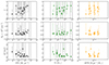 |
Fig. A.1. Best-fit parameters for the 17 SFR-M⋆ stacks for which the spectral fitting resulted in a low reduced-χ2 as a function of the mean SFR, M⋆ and sSFR per SFR-M⋆ bin. |
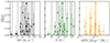 |
Fig. A.2. Ratio of the normalisations of the two components (power-law, APEC) as a function of the mean SFR,M⋆, and sSFR per SFR-M⋆ bin. |
Appendix B: Properties of HEC-eR1 star-forming galaxies with reliable X-ray flux measurements
Properties of HEC-eR1 star-forming galaxies with reliable X-ray flux measurements.
All Tables
Sample selection criteria for the star-forming galaxies within the HEC-eR1 sample.
Sample size in each step of the screening process for the construction of the final HEC-eR1 sample of star-forming galaxies.
Best-fitting model spectral parameters for the average X-ray spectrum of all the HEC-eR1 star-forming galaxies.
Properties of HEC-eR1 star-forming galaxies with reliable X-ray flux measurements.
All Figures
|
Fig. 1. Example of the posterior count distribution of two sources in our sample for which we have reliable and unreliable flux measurement as defined based on the Eq. (1). The red and green error bars indicate the upper and lower bounds of the distribution at the 68% and the 90% C.I., respectively. The vertical black solid line indicates the mode value. |
| In the text | |
|
Fig. 2. Flux distribution in the 0.6–2.3 keV band of the star-forming galaxies in the HEC-eR1 sample as a function of the exposure time. Black stars show the mode value of the source’s intensity for the galaxies with reliable fluxes and their 68% C.I. uncertainties. Grey down arrows show the upper 90% C.I. for the galaxies with uncertain flux measurements. |
| In the text | |
|
Fig. 3. Comparison between the X-ray fluxes measured from the eRASS1 extractions (Sect. 3.3) and those derived from archival Chandra and XMM-Newton observations. The orange line corresponds to the line of equality. We find good agreement with a scatter of ∼0.5 dex, supporting the robustness of the eRASS1 extractions. |
| In the text | |
|
Fig. 4. Distribution of the final clean sample of the secure star-forming HEC-eR1 galaxies in the main sequence plane. In both panels, stars indicate the galaxies with reliable X-ray flux measurements, and the dots the galaxies with uncertain fluxes. The colour-code in the top panel corresponds to the log(D), while in the bottom panel corresponds to the gas-phase metallicity, 12+log(O/H). The diagonal dashed lines indicate three different sSFR values (i.e. sSFR: 10−9, 10−10, and 10−11 M⊙ yr−1/M⊙). The orange solid line shows the main sequence of the star-forming galaxies from Renzini & Peng (2015). Our final sample is well distributed along the SFR-M⋆ plane covering a wide range of distances and gas-phase metallicities. |
| In the text | |
|
Fig. 5. Stacked X-ray spectrum of all the secure star-forming galaxies within the HEC-eR1 sample. The green and red lines show the power-law and hot plasma model components, respectively. The orange line corresponds to the best-fit model. |
| In the text | |
|
Fig. 6. Distribution of SFR-M⋆-D bins on the main sequence plane. Each bin is characterised by the mean SFR and M⋆ of the galaxies contained in each bin. Blue squares correspond to the stacks with reliable X-ray flux measurements based on the X-ray stacking analysis and the blue circles to those with uncertain flux measurements. Black stars show the individual galaxies with reliable X-ray flux measurements and the grey circles the galaxies with uncertain fluxes. The black dashed lines indicate the SFR and M⋆ range of the bins. The diagonal dashed lines indicate three different sSFR values (i.e. sSFR: 10−9, 10−10, and 10−11 M⊙ yr−1/M⊙). |
| In the text | |
|
Fig. 7. Distribution of the estimated background AGN contamination fraction in the SFR-M⋆-D stack bin in our sample. The contamination fraction assuming the eRASS1 flux sensitivity limit of each individual galaxy. The median value of the distribution is 17%. The total surface of the 5 stacks with contamination fraction higher than 50% is significantly higher than all the rest used in our analysis resulting in an overestimation of the background AGN contamination. |
| In the text | |
|
Fig. 8. X-ray luminosity (0.5–2 keV) as a function of the SFR for the stacked data with reliable flux measurements colour-coded with the estimated contamination by the background AGN. Only the stacks with available estimation of the background contamination are shown. For comparison, we overplot the scaling relation from Mineo et al. (2014) (M14). We see that the contamination is independent of the SFR-M⋆-D bins and there is no systematic trend with SFR or LX. The few stacks with very high contamination fraction (> 50%) are due to their total surface which is systematically higher than all the rest used in our analysis resulting in an overestimation of the background AGN contamination. |
| In the text | |
|
Fig. 9. LX versus D for the HEC-eR1 sample of star-forming galaxies. Black stars show the galaxies with reliable flux measurements and lightgray down-arrows, galaxies with uncertain flux measurements. For comparison, we also overplot the normal galaxies from Mineo et al. (2014) and Vulic et al. (2022) as orange triangles and turquoise stars. We also overplot with red contours the galaxy population expected to be observed in the eRASS:8 survey based on the simulation study of Basu-Zych et al. (2020). The dashed and solid lines mark the eRASS1 sensitivity limits at the ecliptic equator and poles respectively. The dotted line indicate the deepest sensitivity of the eROSITA survey which is expected to be reached at the poles of the eRASS:8. These lines are based on the sensitivity values reported in Predehl et al. (2021). |
| In the text | |
|
Fig. 10. LX versus SFR for the HEC-eR1 sample of star-forming galaxies. Black stars show the galaxies with reliable flux measurements and lightgray down-arrows galaxies with uncertain flux measurements. The lines correspond to the limiting LX in each SFR-MD bin, colour-coded by their median distance. Vertical black dashed lines indicate the SFR bins presented in Table 5. The red dashed line shows the standard LX-SFR scaling relation from Mineo et al. (2014) along with the 1σ scatter. |
| In the text | |
|
Fig. 11. Distribution of the LX0.5 − 2 as a function of the SFR and the sSFR. The left panel shows the distribution of all the HEC-eR1 secure star-forming galaxies in the |
| In the text | |
|
Fig. 12. Bootstraps distribution of the |
| In the text | |
|
Fig. 13. Excess of the SFR-M⋆-D stacks with reliable flux measurements from the |
| In the text | |
|
Fig. 14. Comparison of our best-fitted scaling relations with the previous works. The left panel shows the distribution of the SFR-M⋆-D stacks in the |
| In the text | |
|
Fig. 15.
|
| In the text | |
|
Fig. 16. Percentage of LMXB contribution as a function of the SFR (top panel) and the sSFR (bottom panel), respectively. The grey stars represent the individual galaxies with reliable flux measurements and the squares the reliable stacks. The colour-code indicates the logarithm of the number of galaxies that participate in each SFR-M⋆-D stack. The error bars were calculated assuming the lower and upper 68% C.I. of the X-ray luminosity distribution. |
| In the text | |
|
Fig. 17. Distribution of the |
| In the text | |
|
Fig. 18.
|
| In the text | |
|
Fig. 19. Total expected X-ray luminosity (0.5–2 keV) due to the stochastic sampling of the HMXBs XLF from Lehmer et al. (2021) (L21), as a function of SFR. Orange and yellow shaded regions indicate the 99% and the 99.9% C.I. of the expected |
| In the text | |
|
Fig. 20. Total expected LX/SFR distribution due to stochastic sampling of HMXBs XLF as a function of the sSFR. The rhombuses indicate the mean LX/SFR per SFR-M⋆ bin, colour-coded with the gas phase metallicity. The orange and magenta lines correspond to the upper and lower 99%, and 99.9% C.Is. of the HMXBs expected LX/SFR, respectively. Grey dashed line depicts the upper 99.9% C.I of the total expected luminosity accounting for the stochasticity of both, LMXBs and HMXBs. We also overplot with a red line the LX/SFR – sSFR L16 scaling relation, and its corresponding 1σ scatter. |
| In the text | |
|
Fig. 21. LX-SFR distribution of the HEC-eR1 star-forming galaxies with reliable flux measurement colour-coded with the log( |
| In the text | |
|
Fig. 22. Optical spectra of the most X-ray luminous ( |
| In the text | |
|
Fig. 23. Number of detected galaxies with |
| In the text | |
|
Fig. A.1. Best-fit parameters for the 17 SFR-M⋆ stacks for which the spectral fitting resulted in a low reduced-χ2 as a function of the mean SFR, M⋆ and sSFR per SFR-M⋆ bin. |
| In the text | |
|
Fig. A.2. Ratio of the normalisations of the two components (power-law, APEC) as a function of the mean SFR,M⋆, and sSFR per SFR-M⋆ bin. |
| In the text | |
Current usage metrics show cumulative count of Article Views (full-text article views including HTML views, PDF and ePub downloads, according to the available data) and Abstracts Views on Vision4Press platform.
Data correspond to usage on the plateform after 2015. The current usage metrics is available 48-96 hours after online publication and is updated daily on week days.
Initial download of the metrics may take a while.